omputational computational visualization

Copyright: Chandrajit Bajaj, CCV, University of Texas at Austin

ComputationalVisualization

Cente

r

CCV Mannheim Summer School 2002

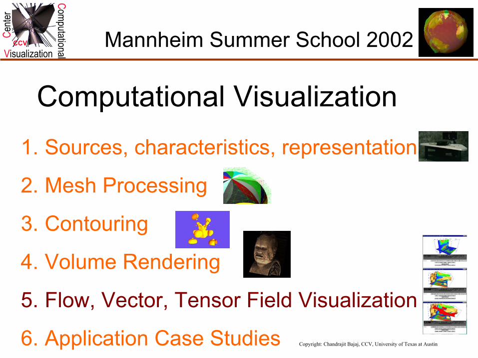
Computational Visualization1. Sources, characteristics, representation

2. Mesh Processing

3. Contouring

4. Volume Rendering

5. Flow, Vector, Tensor Field Visualization

6. Application Case Studies



Cente

r

CCV

Computational Visualization:Flow, Vector, Tensor Field Visualization

Lecture 5



Cente

r

CCV

Outline: Scalar and Vector Topology

•I PROBLEM DOMAIN •Scalar Fields ---- restrictions to surfaces•Vector Fields ---- extensions to functions

on surfaces•Different Grids --- unstructured, curvilinear•II TOPOLOGY COMPUTATION•Critical Points --- nonlinear system solvers; multiplicity, index•Local Analysis --- eigenvalues, newton factorization•Streamlines --- advection; dual stream surfaces

•I PROBLEM DOMAIN •Scalar Fields ---- restrictions to surfaces•Vector Fields ---- extensions to functions

on surfaces•Different Grids --- unstructured, curvilinear•II TOPOLOGY COMPUTATION•Critical Points --- nonlinear system solvers; multiplicity, index•Local Analysis --- eigenvalues, newton factorization•Streamlines --- advection; dual stream surfaces



Cente

r

CCV

Interrogation of Axial Vortices(with G. Blaisdell, Purdue University)

• How is the turbulent kinetic energy produced ?

• Are the production terms of kinetic energy related to the large helical vortices ?

• Do the helical vortices rotate, move axially or remain stationary?

• How is the turbulent kinetic energy produced ?

• Are the production terms of kinetic energy related to the large helical vortices ?

• Do the helical vortices rotate, move axially or remain stationary?



Cente

r

CCV Line Integral Convolution

• Input vector field and texture (white noise)

• Output intensity value on each pixel

• Output image is highly correlated along the streamlines and uncorrelated in directions perpendicular to the streamlines



Cente

r

CCV Line Integral Convolution

vv

dsdt

dtd

dssd

==σσ )(

v• Given a vector field , the streamline equation is

Image intensity at a point x is defined as

∫+

−−=

Ls

LsdsssksTxI 0

0

)())(()( 0σ

where T is the input white noise texture and )(sσ

is the streamline with

xs =)( 0σ

xs =)( 0σ

)(sk is a symmetric filter function.



Cente

r

CCV LIC Example

Input vector field L=20

L=200 L=800



Cente

r

CCV Double LIC

• Original LIC– Random white noise values averaged

along a local streamline.– Flow lines not delineated clearly

• Double LIC– Use the output image of first LIC as the

input of the second LIC– Pixel intensities averaged along a

previously integrated streamline.



Cente

r

CCV Enhanced LIC



Cente

r

CCV Vector Signature Function

• Given two scalar fields U(x, y, z), V(x, y, z)defined over a 3D volume,

• Inner VolumeI(u, v) = Volume( U(x, y, z) <= u and V(x, y, z) <= v})

• Outer VolumeO(x, y) = Volume( U(x, y, z) > u and V(x, y, z) > v}),

where u, v are called isovalues of U, V respectively.• (I, O) is a vector field defined over the domain

{U, V}. It is called a vector signature function.

• Vector signature function can be other properties of the two scalar fields.



Cente

r

CCV

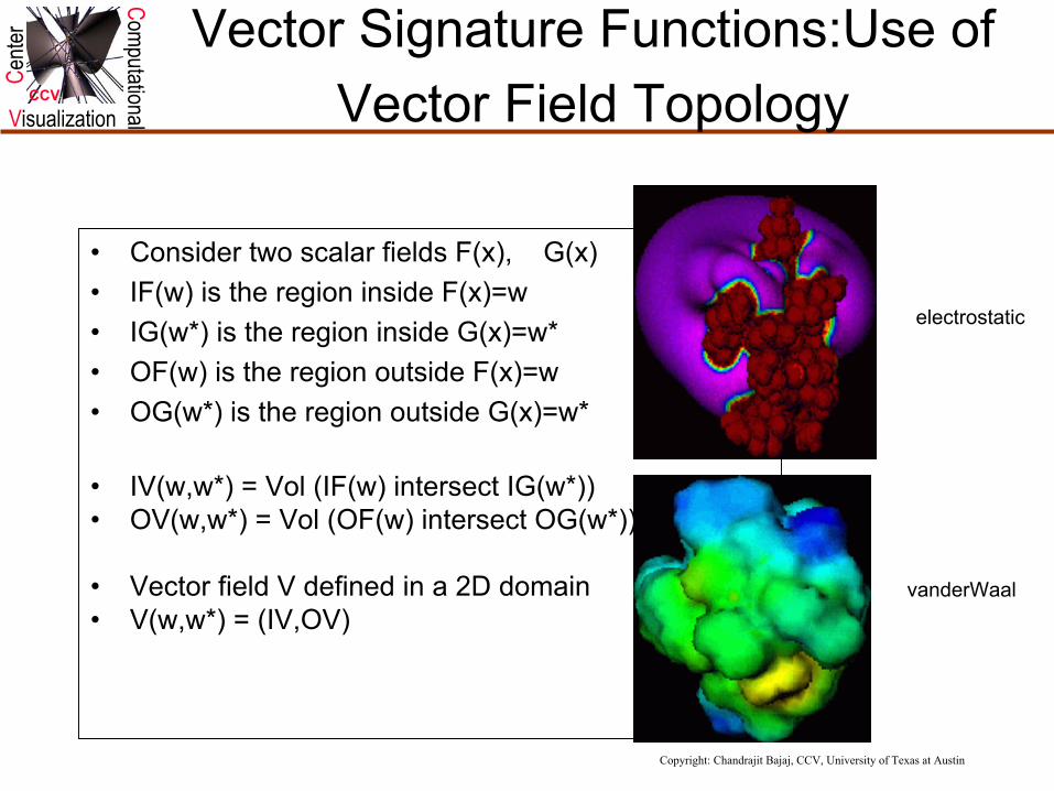
Vector Signature Functions:Use of Vector Field Topology

• Consider two scalar fields F(x), G(x)• IF(w) is the region inside F(x)=w• IG(w*) is the region inside G(x)=w*• OF(w) is the region outside F(x)=w• OG(w*) is the region outside G(x)=w*

• IV(w,w*) = Vol (IF(w) intersect IG(w*))• OV(w,w*) = Vol (OF(w) intersect OG(w*))

• Vector field V defined in a 2D domain• V(w,w*) = (IV,OV)

electrostatic

vanderWaal



Cente

r

CCVVector Correlation Signature Example

Glucose potentials (Electrostatics, vanderWaal)

Inner volume Outer volume

Single LIC Double LIC

electrostatic

vanderWaal



Cente

r

CCV Construction of Vector Topology

• I Detect stationary (critical) points • II Classify critical points• III Link with integral curves of vector

field

• I Detect stationary (critical) points • II Classify critical points• III Link with integral curves of vector

field



Cente

r

CCV 3D Vector Field

Critical Points

First Order Local Analysis at the Critical Points

Eigenstructure of

[ ]),,(),,,(),,,( zyxhzyxgzyxf

0),,(),,(),,(=

zyxhzyxgzyxf

=

zyx

zyx

zyx

hhhgggfff

J



Cente

r

CCV

Vector Local Topology(2D critical point classification)

Spiral Source

Spiral SinkR - - I <>0

CenterR =0 I <>0

Saddle Source

SinkR - - I=0

Spiral SourceR + + I<>0

SaddleR - - I=0

SourceR + + I =0



Cente

r

CCV Vortex Identification



Cente

r

CCV Vortex Core in Turbulent Flow

• Vortex core (red) computed by vector field topology. Green curves are streamlines computed near critical points on the vortex core.

• Vortex core (red) computed by vector field topology. Green curves are streamlines computed near critical points on the vortex core.



Cente

r

CCV Vector Field Visualization

An isocontour of vorticitymagnitude is displayed with partial transparency. The red contour represents a region of positive production term of turbulent kinetic energy. The green contour represents negative production terms.



Cente

r

CCV

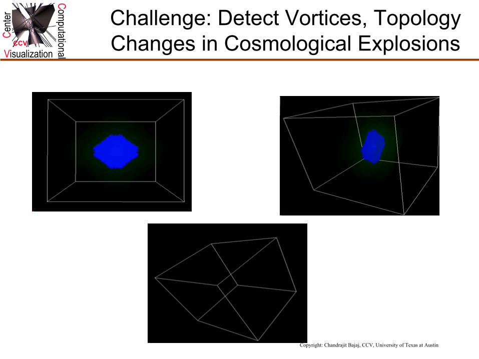
Challenge: Detect Vortices, Topology Changes in Cosmological Explosions



Cente

r

CCV Scalar Field Topology

Pion Collision Simulation

Close-up snapshot of above

Topology of wind speed in a climate model simulation

Topology of a mathematical function reveals information hidden in contour display



Cente

r

CCV 3D Scalar Field

zzzyzx

yzyyyx

xzxyxx

fffffffff

=fH

),,( zyxf

z

y

x

fff

=∇f 0=Critical Points

First Order Local Analysis at the Critical Points

Eigenstructure of



Cente

r

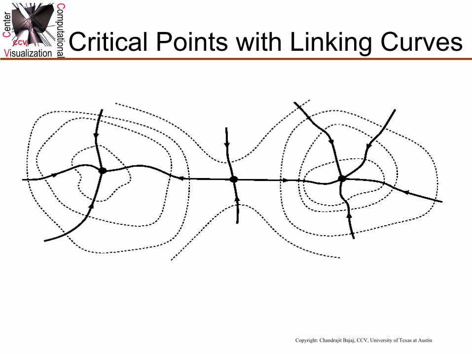
CCV Critical Points with Linking Curves



Cente

r

CCV Integral Curves of Vector Field

dtXdXU =)(

Ref: Dual Stream Functions, David Kenwright’s Thesis1993, AucklandAlso: Bajaj, Xu, Spline Approx. of Algebraic Surface-Surface Intersection Curves, Advances in Comp. Math, 1996

Solution of ODE : Runge-Kutte, 4th Order Integration

Dual Stream Functions for Solenoidal Vector Fields (zero divergence) [Yih1957]

and obey law of mass conservation

Single Stream Functions for 2D incompressible flow (Lagrange1781)

yUp

xUp

∂Ψ∂

=

∂Ψ∂

=

for integral curves0=Ψ∂

gfUp ∇×∇=



Cente

r

CCV

Topology preserving, Finite ElementInterpolants

Open question:What is the true interpolant which does not perturb the topology of the underlying data ?



Cente

r

CCV

Vector Topology in 3D:Topology Preserving Interpolation

Open Questions : Field Topology preservation ?



Cente

r

CCV

Scalar Topology(3D structure enhancement)



Cente

r

CCV

Scalar Topology(Road Map for Data Exploration)



Cente

r

CCV Scalar Topology

dynamic structure tracking



Cente

r

CCV

51-timestep simulation of a Pion Collision (Original 12 data variables over a

rectilinear mesh)

Pion Collison after 3% error-bounded decimation (all variables)

of 60% -85% per timestep

Feature Preserving Decimation of PionCollision



Cente

r

CCV

Topology Preserving Simplification (J. of Computers & Graphics, 1998)

Original Data (130050 tri)7% Error

(90% reduced, 13061 tri)Data Courtesy Tsuyoshi Yamamoto and Hiroyuki Fukuda, Hokkaido University



Cente

r

CCV Gated MRI Closeup

Original Data (130050 tri)7% Error

(90% reduced, 13061 tri)



Cente

r

CCV

To wake up with coffee! Or Mineralwasser !!



Cente

r

CCV

Curves f(x,y) = 0, 2D Scalar Fields

• I Critical Points are Singularities• nodal, cuspidal, tacnodal, higher order• II Classification of singularities• simple: eigenvalues of Hessian of f• higher order: Weierstrass preparation followed by• a Newton factorization both using bivariate Hensel

Lifting• Ref: Abhyankar, Bajaj, Rational Parameteriz. Of Algebraic Curves,

CAGD• Bajaj, Xu, Rational Spline Approx. of Plane Algebraic Curves, J of

Comp. Math, 1995,



Cente

r

CCV

Weierstrass (x^3-x^2+y^2,6)

Newton ((x^2+y^2)^2+3*x^2*y-y^3,0,4)

localpower2d (x^3-x^2+_y^2,s,6,0,0)

•••

•••

•••

Weierstrass, Newton and Pade’



Cente

r

CCV

Global Parameterization of Real Algebraic Curves

• Computation of Real Curve Genus

• Real Rational Parameterization of Real Curves of Genus 0

Ref: • Abhyankar, Bajaj, Computer Aided Design 1987• Recio, Sendra, Winkler

J. of Symbolic Computation, 1995, 1997



Cente

r

CCV

Piecewise Rational Parameterizations of Real Algebraic Curves

ProblemGiven a real algebraic plane curve C: f(x, y) = 0 of degree d and of arbitrary genus, a box B defined by

an error bound ,and integers m,n with construct a C0 orC1 continuous piecewise rational -approximation of all portions of C within the given bounding box B, with each rational function of degree and degree

.

},,),{( δγβα ≤≤≤≤ yxyx 0>εdnm ≤+ε

i

i

QP mPi ≤

nQi ≤



Cente

r

CCV Sketch of Algorithm

Compute all intersections of C within the given bounding box B and also the tracing direction at these points. Next, compute all singular points S and x-extreme points T in the bounded plane curve CB.

Compute a Newton factorization for each singular point (xi,yi)in S and obtain a power series representation for each analytic branch of C at (xi, yi ) and given by

1.

2.

ik

i sxsX +=)(,)( )(

0ji

jj scSY ∞=∑= i

i yc =)(0 (2.1)

or

,~)( )(0

jijj

scsX ∞=

∑= ii xc =)(

0~

(2.2)

iki

sysY +=)(



Cente

r

CCV

3. Without loss of generality, consider the case where the analytic branch at the singularity is of type (2.1). Compute

the (m,n) Padé approximation of Y(s). That is )()(

sQsP

mn

mn

)()()()( 1++=− nm

mn

mn sOsYsQsP

4. Compute β > 0 a real number, corresponding to points and

on the analytic branch of the original curve C, such that is convergent for

))(~),(~( ββ YyXx ii == ))(ˆ),(ˆ( ββ −=−= YyXx ii

)()(

sQsP

mn

mn [ ]ββ ,−∈s

Sketch of Algorithm (contd)



Cente

r

CCV

5. Modify to is C1 continuous approximation of Y(s) on [0, β]

)(/)( sQsP mnmn )(~/)(~ sQsP mnmn

6. Denote the set of all the points the set T and the boundary points of CB by V. The curve CB yields a naturalgraph G having V, as its vertex set and the set of curve segments of CB joining any pair of points in V, as its edge setE. Now starting from each (simple) point in V we traceout the graph G, approximating each of its edges E by C1

continuous piecewise rational curves.

),ˆˆ(),~~( ,, iiii yxyx

)( , ii yx

Sketch of Algorithm (contd)



Cente

r

CCV

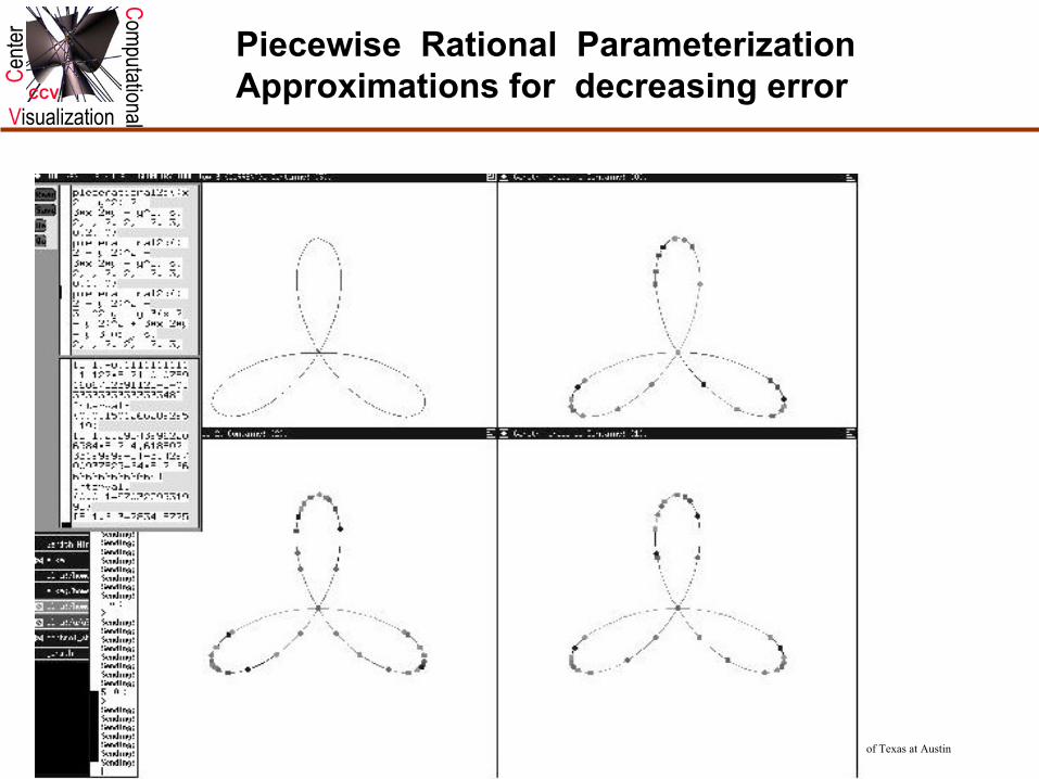
Piecewise Rational Parameterization Approximations for decreasing error



Cente

r

CCV

Hensel Lifting

Consider of degree d and monic in y),( yxf

⋅⋅⋅++⋅⋅⋅++= kk xyfxyfyfyxf )()()(),( 10

We wish to compute real power series factors g(x,y) and h(x,y) = g(x,y)h(x,y)The technique of Hensel lifting allows one to reconstruct the power series factors

⋅⋅⋅++⋅⋅⋅++= ii xygxygygyxg )()()(),( 10

⋅⋅⋅++⋅⋅⋅++= jj xyhxyhyhyxh )()()(),( 10

From initial factors )()()(),0( 000 yhygyfyf ==

Expansion at Singular Points



Cente

r

CCV

Weierstrass Factorization

A Weierstrass power series factorization is of the form

,)()(),0()(00 )(

100

yh

e

yg

yyaayfyf ⋅⋅⋅++==

Where g(x,y) is a unit power series

The Weierstrass preparation can be achieved via Hensel Lifting from the initial factors:

),(

01

1 ))()((),(),(yxh

ee

e xayxayyxgyxf +⋅⋅⋅++= −−



Cente

r

CCV

Newton Factorization

Let

)()(),( 01

1 xayxayyxh ee

e +⋅⋅⋅++= −−

Then it is possible to factor h(x,y) into real linear factors of the type using Hensel Lifting

)))(((),( 1 tyyxh iei η−∏= =



Cente

r

CCV Surfaces f(x,y,z) = 0, 3D Scalar Fields

• I Critical Points (& Curves) are Singularities• points: difficult ?• curves: nodal, cuspidal, tacnodal, higher order

• II Classification of singularities• simple points: eigenvalues of Hessian of f• higher order points : ??• Curves : some similar to singular points on curves. Others ?

• Ref: Bajaj, Xu, Rational Spline Approx. of Real Algebraic Surfaces, J of Symbolic Computation, 1997



Cente

r

CCV

Topology Preserving Spline Approximations and Display of Real Algebraic Surfaces



Cente

r

CCV

Global Rational Parameterization for Real Algebraic Surfaces

• Computation of Arithmetic Genus, Second Plurigenus

• Parametrization of Real Surfaces satisfying Castelnuovo criterion for rationality ?

• Ref: J. Schicho, Journal of Symbolic Computation 1997



Cente

r

CCV

Given two skew lines

=

)()()(

)(1

1

1

1

1

uzuyux

u and

=

)()()(

)(1

2

2

2

2

vzvyvx

v

On the cubic surface f(x, y, z) = 0, the cubic rational parametrization formula for a point p(u, v) on the surface is

),(),()(1),()(1),(11

),(),(),(

),( 2121

vubvuavvubuvua

baba

vuzvuyvux

vu++

=++

=

=Ρ

where

⋅−⋅∇==−⋅∇==

)](1)(1[))(1(),()](1)(1[))(1(),(

211

212

vuvfvubbvuvfvuaa

Global Rational Parameterization of Non-Singular Real Cubic Surfaces



Cente

r

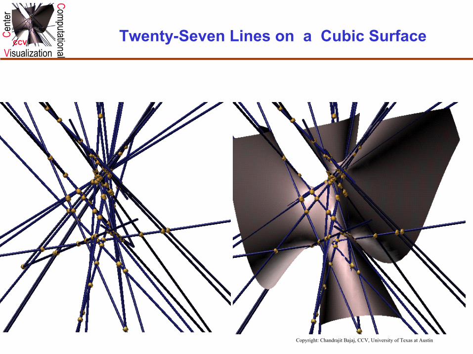
CCV Twenty-Seven Lines on a Cubic Surface



Cente

r

CCV

0)ˆ,ˆ(ˆ)ˆ,ˆ(ˆ32 =+ yxgyxf

THEOREM 1. The polynomial P81(t) obtained by taking the resultant of and factors as , where is the denominator of K(t) and L(t), and P(6)(t) is the numerator of .

2f 3g 66

632781 )]([)]()[()( tPtPtPtP =

+′′= 33 )( tBtP AtDtF ′′+′′+′′ 2

]))()[()()(( 236 tPtStPtS =

THEOREM 2. Simple real roots of P27(t) = 0 correspond to reallines on the surface.

Twenty-Seven Lines on the Cubic Surface

(Schlafi’s double-six)



Cente

r

CCV

Rational Parametrization of Cubic A- Patches in BB form

Ref: (ACM Transactions on Graphics’97)



Cente

r

CCV Triangulation and Display of Rational Parametric Surfaces

A rational parametric surface is defined by the three rational functions:

,),(),(),(

tsWtsXtsx = ,

),(),(),(tsWtsYtsy =

),(),(),(tsWtsZtsz =

1. Domain poles. The map yields a divide by zero at points satisfying W(s,t) = 0, the pole of the rational functions. These domain poles are algebraic curves.

2. Domain base points. The map is undefined at points satisfying X(s,t) = Y(s,t) = Z(s,t) =W(s,t) = 0. There are finitely many such points, called domain base points.

3. Surface singularities. The given rational surface may be singular.

4. Complex parameter values. Some real points of the surface are generated only by complexParameter values.

5. Infinite parameter values. Some finite points of the surface are generated only by infinite parameter values.



Cente

r

CCV

THEOREM 1 Let (a,b) be a base point of multiplicity q. Then for any m ∈ R, the image of a domain point approaching (a,b) along a line of slope m is given by (X(m),Y(m),Z(m)W(m) =

)),(),(( 00i

iiq

qqi

iiiq

qqi m

iq

bats

Xmiq

bats

X

∂∂

∂∑⋅⋅⋅

∂∂

∂∑ −=−=

COROLLARY 1 If the curves X(s,t) = 0, …,W(s,t) = 0 share t tangent lines at (a,b),then the seam curve (X(m),Y(m),Z(m),W(m)) has degree q-t. In particular, if X(s,t) = 0have identical tangents at (a,b), then for all m ∈ R the coordinates (X(m),…,W(m))represent a single point.

Ref: Bajaj, Royappa Triangulation and Display of Arbitrary Rational SurfacesIEEE Visualization Conference 1994

Image of a Base Point is a Rational Curve



Cente

r

CCV



Cente

r

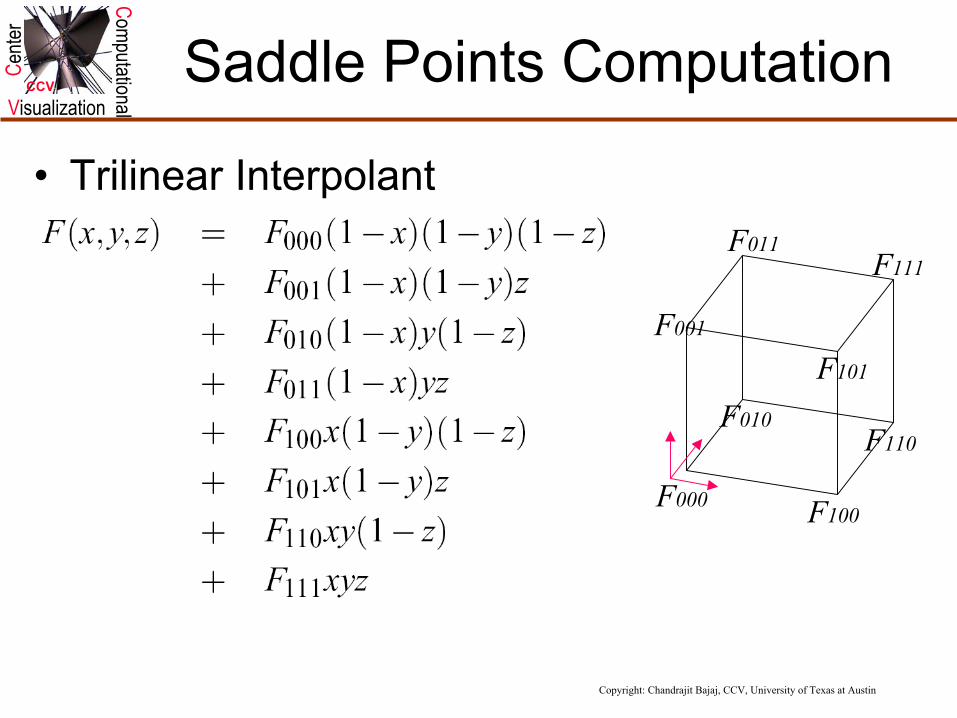
CCV Saddle Points Computation

F001

F011F111

F101

F000 F100

F010F110

• Trilinear Interpolant



Cente

r

CCV

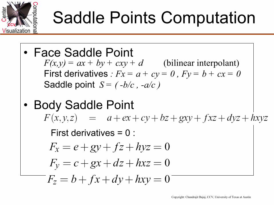
• Face Saddle Point

• Body Saddle Point

Saddle Points Computation

F(x,y) = ax + by + cxy + d (bilinear interpolant)First derivatives : Fx = a + cy = 0 , Fy = b + cx = 0Saddle point S = ( -b/c , -a/c )

First derivatives = 0 :



Cente

r

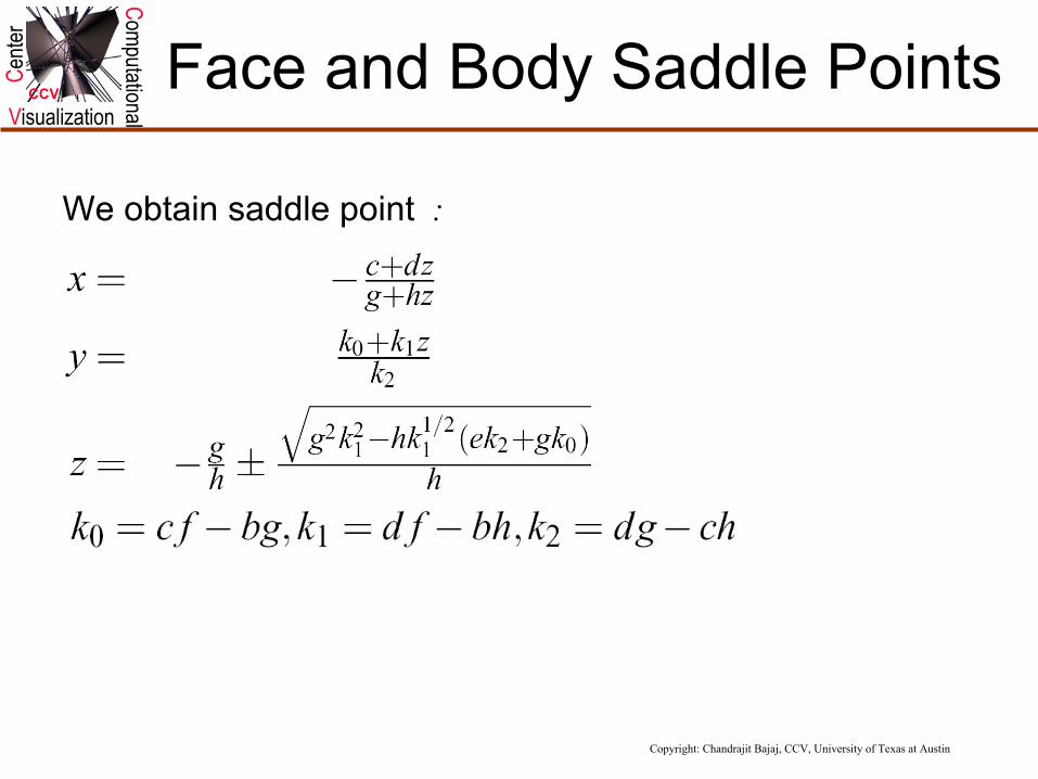
CCV Face and Body Saddle Points

We obtain saddle point :



Cente

r

CCV Decision on Topology

• Resolving Face Ambiguity– Ambiguity

– Decision based on the value s of saddle point

s is black s is white



Cente

r

CCV

–Decision based on the value of saddle points

• Resolving Internal Ambiguity– Ambiguity

(i) s is black tunnel(ii) s is white two pieces



Cente

r

CCV31 Cases



Cente

r

CCV

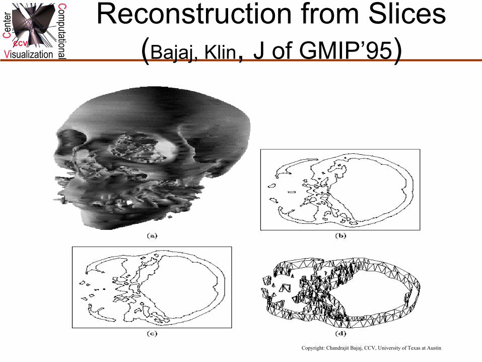
Reconstruction from Slices(Bajaj, Klin, J of GMIP’95)



Cente

r

CCV

Topologically correct reconstruction from Volumetric Images

Points cloud

Knee JointA-Patch BEM

Signed DistanceAlpha-Solid



Cente

r

CCV

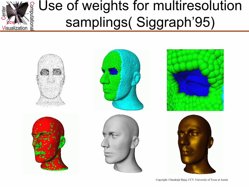
Use of weights for multiresolutionsamplings( Siggraph’95)



Cente

r

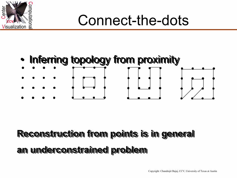
CCV Connect-the-dots

• Inferring topology from proximity• Inferring topology from proximity

Reconstruction from points is in generalan underconstrained problemReconstruction from points is in generalReconstruction from points is in general

anan underconstrainedunderconstrained problemproblem



Cente

r

CCV Sampling a 1-manifold

Neighborhoodintersectionproperty

Samplingdensityproperty

Yes No



Cente

r

CCV

Sampling and Reconstruction Theorem (IJCGA’96)

• Let B be a compact 1-manifold without boundary, and S a sampling. If

• 1. for any closed disk D of radius r, B �D is either (a) empty, (b) a single point, (c) an interval;

• 2. an open disk of radius r centered on B contains at least one point of S

• then the alpha-shape W�, � = r2, is homeomorphicto B and

• max min || p - q || < r• p �W� q � B

• Let B be a compact 1-manifold without boundary, and S a sampling. If

• 1. for any closed disk D of radius r, B �D is either (a) empty, (b) a single point, (c) an interval;

• 2. an open disk of radius r centered on B contains at least one point of S

• then the alpha-shape W�, � = r2, is homeomorphicto B and

• max min || p - q || < r• p �W� q � B



Cente

r

CCV

Feature Preserving Reconstruction of CAD Models

PointsPoints Triangle meshTriangle mesh Reduced meshReduced mesh Smooth modelSmooth model

3D3D DelaunayDelaunay tri. tri. and and α−α−solidsolid

MeshMeshreductionreduction

AA--patchpatchfittingfitting



Cente

r

CCV Feature Surface Fitting

– Uses cubic A-patches (algebraic patches)

– C1 continuity

– Uses cubic A-patches (algebraic patches)

– C1 continuity

• Sharp features (corners, sharp curved edges)

• Singularities

•• Sharp features (corners, Sharp features (corners, sharp curved edges)sharp curved edges)

•• SingularitiesSingularities



Cente

r

CCV

Feature Preserving Model Reconstruction

Input Data2*104 pts

α-solid17786 triangles

Reduced mesh248 triangles

A-patch tetrahedralsupport mesh

A-patch fitface- and edge-patches

Reconstructedmodel



Cente

r

CCV Sharp Features Reconstruction:



Cente

r

CCV Further reading• Line integral convolution• Brian Cabral and Leith Casey Leedom, Imaging vector fields using line integral convolution, Proceedings of the 20th annual

conference on Computer graphics, p 263-270

• Fast Line Integral Convolution• Detlev Stalling and Hans-Christian Hege, Fast and resolution independent line integral convolution, Proceedings of the 22nd

annual ACM conference on Computer graphics, p 249-256• Rainer Wegenkittl and Eduard Gröller, Fast oriented line integral convolution for vector field visualization via the Internet,

Proceedings of the conference on Visualization '97, p 309-316

• Flow Fields• Han-Wei Shen; Kao, D.L., A new line integral convolution algorithm for visualizing time-varying flow fields, Visualization and

Computer Graphics, IEEE Transactions on , Volume: 4 Issue: 2 , April-June 1998, Pages 98 -108• Interrante, V.; Grosch, C., Strategies for effectively visualizing 3D flow with volume LIC, Visualization '97., Proceedings , 1997 p

421 -424, • Wegenkittl, R.; Groller, E.; Purgathofer, W., Animating flow fields: rendering of oriented line integral convolution, Computer

Animation '97 , 1997 p 15 -21• Forssell, L.K.; Cohen, S.D., Using line integral convolution for flow visualization: curvilinear grids, variable-speed animation,

and unsteady flows, Visualization and Computer Graphics, IEEE Transactions on , Volume: 1 Issue: 2 , June 1995 p 133 -141• Forssell, L.K.,Visualizing flow over curvilinear grid surfaces using line integral convolution, Visualization, 1994 p 240 -247

• Others• Han-Wei Shen, Christopher R. Johnson and Kwan-Liu Ma, Visualizing vector fields using line integral convolution and dye

advection, Proceedings of the 1996 symposium on Volume visualization, Page 63• Verma, V.; Kao, D.; Pang, A., PLIC: bridging the gap between streamlines and LIC, Visualization 1999, p 341 -541• Gerik Scheuermann, Holger Burbach and Hans Hagen, Visualizing planar vector fields with normal component using line

integral convolution, Proceedings of the conference on Visualization '99, Pages 255-261• C. Rezk-Salama, P. Hastreiter, C. Teitzel and T. Ertl, Interactive exploration of volume line integral convolution based on 3D-

texture mapping, Proceedings of the conference on Visualization '99, Pages 233-240• de Leeuw, W.; van Liere, R., Comparing LIC and spot noise, Visualization '98. Proceedings , 1998 p 359 -365• Ming-Hoe Kiu; Banks, D.C., Multi-frequency noise for LIC, Visualization '96. Proceedings. , 1996 p 121 -126



Cente

r

CCV Further Reading

•Bader(1990)- gradient fields in molecular systems.•Bergman, Rogowitz, and Treinish(1995) - enhancing colormapped visualiztion.•Gershon(1992) - Generalized Animation•Jones and Chen(1994), Lorensen and Cline(1987), Wilhelms andGelder(1990) - isocontours in 2d and 3d scalar data.•Fowler and Little(1979) - detecting ridges and valleys.• McCormack, Gahegan, Roberts, Hogg, Hoyle(1993) - detecting drainage patterns in geographic terrain.•Interrante, Fuchs, and Pizer(1995) - enhancing surface displays•Itoh and Koyamada(1994) - Isocontour extraction.•Helman and Hesselink(1991), Globus (1991), Asimov (1993) - vector field topology.•Yih (1957), Kenwright, Mallinson (1992) - dual stream functions

•Bader(1990)- gradient fields in molecular systems.•Bergman, Rogowitz, and Treinish(1995) - enhancing colormapped visualiztion.•Gershon(1992) - Generalized Animation•Jones and Chen(1994), Lorensen and Cline(1987), Wilhelms andGelder(1990) - isocontours in 2d and 3d scalar data.•Fowler and Little(1979) - detecting ridges and valleys.• McCormack, Gahegan, Roberts, Hogg, Hoyle(1993) - detecting drainage patterns in geographic terrain.•Interrante, Fuchs, and Pizer(1995) - enhancing surface displays•Itoh and Koyamada(1994) - Isocontour extraction.•Helman and Hesselink(1991), Globus (1991), Asimov (1993) - vector field topology.•Yih (1957), Kenwright, Mallinson (1992) - dual stream functions



Cente

r

CCV Further Reading

• J. Hultquist, Construcing stream surfaces in steady 3D vector fields,proceedings of visualization ‘92

• J. Van Wijk, implicit stream surfaces, proceedings of visualization ‘93• Scheurman, Hagen, Rockwood, constructing degenerate vector fields,

proceedings of visualization ‘97• Bajaj, Pascucci, Schikore, scalar topology for enhanced visualization,

proceedings of visualization ‘98

• J. Hultquist, Construcing stream surfaces in steady 3D vector fields,proceedings of visualization ‘92

• J. Van Wijk, implicit stream surfaces, proceedings of visualization ‘93• Scheurman, Hagen, Rockwood, constructing degenerate vector fields,

proceedings of visualization ‘97• Bajaj, Pascucci, Schikore, scalar topology for enhanced visualization,

proceedings of visualization ‘98



Cente

r

CCV Mannheim Summer School 2002

Computational Visualization1. Sources, characteristics, representation

2. Mesh Processing

3. Contouring

4. Volume Rendering

5. Flow, Vector, Tensor Field Visualization

6. Application Case Studies

omputational computational visualization

Documents