olar and planetary oscillation ontrol on...

SOLAR AND PLANETARY OSCILLATION

CONTROL ON CLIMATE CHANGE: Hind-cast, Forecast and a

Comparison with the CMIP5 GCMs

by Nicola Scafetta

SPPI REPRINT SERIES ♦ July 2, 2013

http://education.kqed.org/edspace/files/2013/01/800px-Solar_system_a-e1357839271803.jpg

MULTI-SCIENCE PUBLISHING CO. LTD.5 Wates Way, Brentwood, Essex CM15 9TB, United Kingdom

Reprinted from

ENERGY &ENVIRONMENT

VOLUME 24 No. 3 & 4 2013

SOLAR AND PLANETARY OSCILLATION CONTROL ON CLI-MATE CHANGE: HIND-CAST, FORECAST AND A COMPARI-

SON WITH THE CMIP5 GCMS

by

Nicola Scafetta (USA)

455

SOLAR AND PLANETARY OSCILLATION CONTROL ONCLIMATE CHANGE: HIND-CAST, FORECAST AND A

COMPARISON WITH THE CMIP5 GCMS

Nicola ScafettaActive Cavity Radiometer Irradiance Monitor (ACRIM) Lab, Coronado, CA 92118, USA,

& Duke University, Durham, NC 27708, USAemail: [email protected]

ABSTRACTGlobal surface temperature records (e.g. HadCRUT4) since 1850 are characterizedby climatic oscillations synchronous with specific solar, planetary and lunarharmonics superimposed on a background warming modulation. The latter isrelated to a long millennial solar oscillation and to changes in the chemicalcomposition of the atmosphere (e.g. aerosol and greenhouse gases). However,current general circulation climate models, e.g. the CMIP5 GCMs, to be used inthe AR5 IPCC Report in 2013, fail to reconstruct the observed climaticoscillations. As an alternate, an empirical model is proposed that uses: (1) aspecific set of decadal, multidecadal, secular and millennial astronomic harmonicsto simulate the observed climatic oscillations; (2) a 0.45 attenuation of the GCMensemble mean simulations to model the anthropogenic and volcano forcingeffects. The proposed empirical model outperforms the GCMs by better hind-casting the observed 1850-2012 climatic patterns. It is found that: (1) about 50-60% of the warming observed since 1850 and since 1970 was induced by naturaloscillations likely resulting from harmonic astronomical forcings that are not yetincluded in the GCMs; (2) a 2000-2040 approximately steady projectedtemperature; (3) a 2000-2100 projected warming ranging between 0.3 oC and 1.6oC , which is significantly lower than the IPCC GCM ensemble mean projectedwarming of 1.1 oC to 4.1 oC ; (4) an equilibrium climate sensitivity to CO2 doublingcentered in 1.35 oC and varying between 0.9 oC and 2.0 oC.

1. INTRODUCTIONSince 1850 the global surface temperature (GST) increased by 0.8-0.85 oC , andsince the 1970s by 0.5-0.55 oC . Figure 1 depicts the HadCRUT4 (1850-2012) GSTrecord1 [1]. The observed secular warming occurred during a period of increasingatmospheric concentrations of greenhouse gases (GHG), especially CO2 and CH4,likely due to human emissions [2]. Current general circulation models (GCMs)interpret that anthropogenic climatic forcings caused more than 90% of the global1http://www.metoffice.gov.uk/hadobs/hadcrut4/

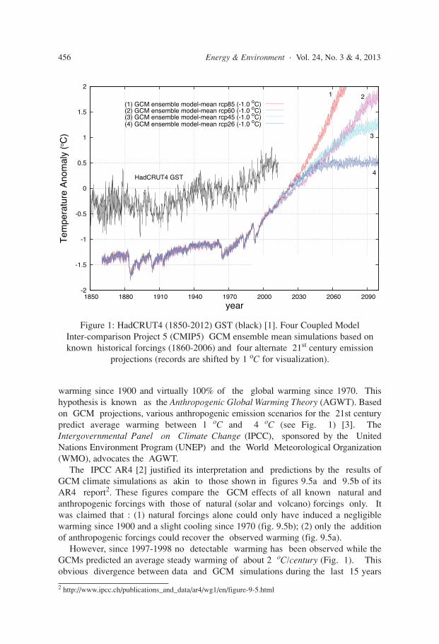
warming since 1900 and virtually 100% of the global warming since 1970. Thishypothesis is known as the Anthropogenic Global Warming Theory (AGWT). Basedon GCM projections, various anthropogenic emission scenarios for the 21st centurypredict average warming between 1 oC and 4 oC (see Fig. 1) [3]. TheIntergovernmental Panel on Climate Change (IPCC), sponsored by the UnitedNations Environment Program (UNEP) and the World Meteorological Organization(WMO), advocates the AGWT.

The IPCC AR4 [2] justified its interpretation and predictions by the results ofGCM climate simulations as akin to those shown in figures 9.5a and 9.5b of itsAR4 report2. These figures compare the GCM effects of all known natural andanthropogenic forcings with those of natural (solar and volcano) forcings only. Itwas claimed that : (1) natural forcings alone could only have induced a negligiblewarming since 1900 and a slight cooling since 1970 (fig. 9.5b); (2) only the additionof anthropogenic forcings could recover the observed warming (fig. 9.5a).

However, since 1997-1998 no detectable warming has been observed while theGCMs predicted an average steady warming of about 2 oC/century (Fig. 1). Thisobvious divergence between data and GCM simulations during the last 15 years

456 Energy & Environment · Vol. 24, No. 3 & 4, 2013

Figure 1: HadCRUT4 (1850-2012) GST (black) [1]. Four Coupled ModelInter-comparison Project 5 (CMIP5) GCM ensemble mean simulations based onknown historical forcings (1860-2006) and four alternate 21st century emission

projections (records are shifted by 1 oC for visualization).

2 http://www.ipcc.ch/publications_and_data/ar4/wg1/en/figure-9-5.html

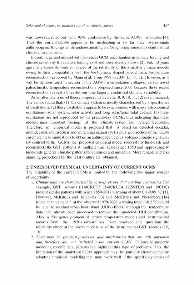
was, however, ruled out with 95% confidence by the same AGWT advocates [4].Thus, the current GCMs appear to be misleading in so far they overestimateanthropogenic forcings while underestimating and/or ignoring some important naturalclimatic mechanisms.

Indeed, large and unresolved theoretical GCM uncertainties in climate forcing andclimate sensitivity to radiative forcing exist and were already known [2]; but, 13 yearsago many scientists were convinced of the reliability of the available climate modelsowing to their compatibility with the hockey-stick shaped paleoclimatic temperaturereconstructions proposed by Mann et al. from 1998 to 2004 [5, 6, 7]. However, as itwill be demonstrated in section 3, the AGWT interpretation collapses versus novelpaleoclimatic temperature reconstructions proposed since 2005 because these recentreconstructions reveal a three-to-four time larger preindustrial climatic variability.

As an alternate, a novel theory proposed by Scafetta [8, 9, 10, 11, 12] is summarized.The author found that: (1) the climate system is mostly characterized by a specific setof oscillations; (2) these oscillations appear to be synchronous with major astronomicaloscillations (solar system, solar activity and long solar/lunar tidal cycles); (3) theseoscillations are not reproduced by the present-day GCMs, thus indicating that thesemodels miss important forcings of the climate system and related feedbacks.Therefore, an empirical model is proposed that is based on detected decadal,multidecadal, multisecular and millennial natural cycles plus a correction of the GCMensemble mean simulations to obtain an anthropogenic plus volcano climatic signature.By contrast to the GCMs, the proposed empirical model successfully hind-casts andreconstructs the GST patterns at multiple time scales since 1850 and approximatelyhind-casts general climatic patterns for centuries and millennia. More reliable and lessalarming projections for the 21st century are obtained.

2. UNRESOLVED PHYSICAL UNCERTAINTY OF CURRENT GCMSThe reliability of the current GCMs is limited by the following five major sourcesof uncertainty:

1. Climate data are characterized by various errors that can bias composites. Forexample, GST records (HadCRUT3, HadCRUT4, GISSTEM and NCDC)present similar patterns with a net 1850-2012 warming of about 0.8-0.85 oC [1].However, McKitrick and Michaels [13] and McKitrick and Nierenberg [14]found that up to half of the observed 1979-2002 warming trend (~0.2 oC) couldbe due to residual urban heat island (UHI) effects, although the temperaturedata had already been processed to remove the (modeled) UHI contribution.Also a divergence problem of proxy temperature models and instrumentalrecords from the 1950s onward has been observed and questions thereliability either of the proxy models or of the instrumental GST records [15,16].

2. There may be physical processes and mechanisms that are still unknownand, therefore, are not included in the current GCMs. Failures in properlymodeling specific data patterns can highlight this type of problems. If so, thelimitation of the analytical GCM approach may be partially circumvented byadopting empirical modeling that may work well if the specific dynamics of

Solar and planetary oscillation control on climate change 457

the conjectured unknown mechanisms are somehow identified, although thephysical details of the mechanisms themselves may remain unknown.Empirical modelling is how ocean tides have been forecast since antiquity [17,18, 19, 20, 21].

3. The failure of GCMs may be due to not predictable chaos, internal variabilityand missing forcings of the climate system. For example, since 2000 nowarming has been observed while the IPCC GCMs predicted on average asteady warming of about 2 oC/century [10]. Meehl et al. [22] speculated thatsuch GST hiatus periods could be caused by unforced internal climaticvariability such as occasionally deep ocean heat uptakes. However, theiradopted CCSM4 GCM did not predicted the steady temperature observed from2000 to 2012, and produces only hiatus periods in 2040-2050 and 2070-2080.Essentially, because of internal dynamical chaos, it is claimed that GCMs canonly statistically, that is in the ensemble of their simulations, vaguelyreproduce the observational data pattern means. Alternatively, other authorspostulated that the same post 2000 GCM-GST discrepancy was the effectof small volcanic eruptions or Chinese aerosols [23]. This interpretationwas proposed despite the fact that no increase in aerosol concentration hasbeen observed since 1998 [24]. So, the issue is quite open and confused.

4. Radiative climate forcings used in the GCMs are characterized by very largeuncertainties. The IPCC AR4 [2] (AR4 WG1 2.9.1 “Uncertainties in RadiativeForcing”3 ) classifies the level of scientific understanding of 11 out of 16forcing agent categories as either low or very low. For example, figure SPM24

of the IPCC AR4 [2] estimates a 1750-2005 net anthropogenic radiative forcingbetween 0.6 and 2.4 W/m2 and the total solar irradiance forcing between 0.06and 0.30 W/m2. Given this large forcing uncertainty, GCM modelers couldarbitrarily adjust internal parameters and forcing functions, such as the veryuncertain aerosol forcing, to improve the fit of their models to the data.Indeed, an inverse correlation was found between the GCM modeled climatesensitivity and total anthropogenic forcing [25, 26].

5. The current equilibrium climate sensitivity to radiative forcing is extremelyuncertain. The IPCC AR4 [2] suggests that a doubling of atmospheric CO2concentrations would induce a most likely warming in the range of 2-4.5 oCaveraging to about 3 oC, which is about the average value simulated by theGCMs. The total range spans between 1-9 oC (see Box 10.2-fig. 1 in IPCCAR4 [2])5. In fact, while the greenhouse properties of CO2 can beexperimentally determined (without water vapor and cloud feedbacks, doublingof CO2 has a forcing of about 3.7 W/m2 causing about 1 oC warming [27]), thestrength of the adopted climatic feedbacks can not be tested experimentally,and is indirectly estimated in various ways. Some empirical studies suggestthat the real climate sensitivity may be as low as 0.5-1.3 oC [28, 29].


3 http://www.ipcc.ch/publications_and_data/ar4/wg1/en/ch2s2-9-1.html4 http://www.ipcc.ch/publications_and_data/ar4/wg1/en/figure-spm-2.html5 http://www.ipcc.ch/publications_and_data/ar4/wg1/en/box-10-2-figure-1.html

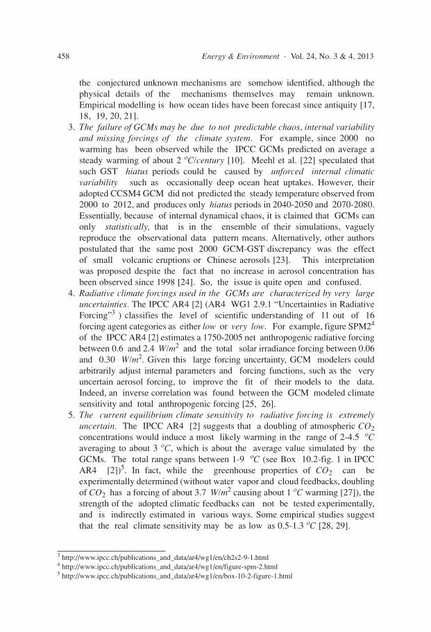
The GCM physical uncertainties appear to be monstrous [30]. It islegitimate to question whether current GCMs implement all relevant physicalmechanisms and whether their simulations and projections can be trusted. Forexample, assuming an equilibrium climate sensitivity range of 2-4.5 oC, the netclimatic forcing adopted by the GCMs would predict a 1850-2012 net warming ofabout 0.57-1.3 oC, while with a climate sensitivity of 1-9 oC, it would be in therange of 0.28-2.6 oC. As shown in Figure 2, estimated uncertainties diverge in modelpredictions after 100 years progressively significantly larger than from the datapatterns that the models attempt to reconstruct. Thus, the performance and physicalreliability of these GCMs cannot be verified within a viable accuracy while it isalways possible to adjust some model parameters or some forcing functions to obtainresults that, at a first sight, appear to reconstruct the temperature warming.

Contrary to what Knutti and Sedlacek [3] claimed, an ensemble agreementbetween different GCMs is not a guarantee of their physical reliability implying agreater confidence in their projections since all models may simply reach the sameerroneous conclusion by mistaking or missing the same physical mechanisms. Thescientific method requires that comparisons must be made with observations and notonly between models. Let us see what the data tell us.


Figure 2: HadCRUT4 GST record (red) vs. the CMIP5 (rcp60) ensemble meansimulation (black). Uncertainty ranges refer to equilibrium climate sensitivity to CO2

doubling spanning 2-4.5 oC (yellow), and 1-9 oC (cyan).

3. AGWT AGREES ONLY WITH OUTDATED HOCKEY-STICKPALEOCLIMATIC TEMPERATURE RECONSTRUCTIONSWhy did scientists supporting the IPCC accept the results of GCMs and theAGWT despite the well-known large uncertainties discussed above? This needsclarification.

In 1998-1999 Mann et al. [5, 6] published preliminary paleoclimatic GSTreconstructions for the last 1000 years suggesting that from the Medieval WarmPeriod (MWP) (900-1400) to the Little Ice Age (LIA) (1400-1800) there was acooling of ~ 0.2 oC opposed to a drastic temperature increase of ~ 1 oC since 1900.The shape of his GST resembles a hockey stick. Despite the fact that historicallydocumented climate changes (e.g. the Viking settlements in Greenland between 900AD and 1400 AD, and many other well-documented world-wide events [31])contradict this hockey-stick graph that contradicts even the IPCC First AssessmentReport (FAR, fig. 7.1, 1990)6 [32], Mann’s GST was considered trustworthy.

Several groups [7, 33, 34] used energy balance models to interpret the hockey-sticktemperature graphs and concluded that the climate is poorly sensitive to solar changesand that the post-1900 warming is almost entirely caused by anthropogenic forcing.In 2000 Crowley [7] stated: The very good agreement between models and data inthe pre-anthropogenic interval also enhances confidence in the overall ability ofclimate models to simulate temperature variability on the largest scales. Sinceunderlying climate models were able to hind-cast the hockey-stick proxy temperaturereconstructions covering the last 1000 years, in 2001 the IPCC AR-3 [35]7 couldpromote AGWT.

However, since 2005 a number of studies confirmed the doubts of Soon andBaliunas [36] about a diffused MWP and demonstrated: (1) Mann’s algorithmcontained a mathematical error that nearly always produces hockey-stick shapes evenfrom random data [37]; (2) a global pre-industrial temperature variability of about0.4-1.0 oC between the MWP and the LIA [16, 38, 39, 40, 41, 42]; (3) theexistence of a millennial climatic oscillation observed throughout the Holocene thatcorrelates with the millennial solar oscillation [11, 43, 44, 45, 46, 47] and agreesbetter with historical inferences [31]. Indeed, since 2001 it was clear that the climateof the last 1000 years could have been influenced by a large millennial climaticoscillation induced by solar activity [43, 44]. Nevertheless, numerous climatescientists claimed that the MWP affected only the North Atlantic.

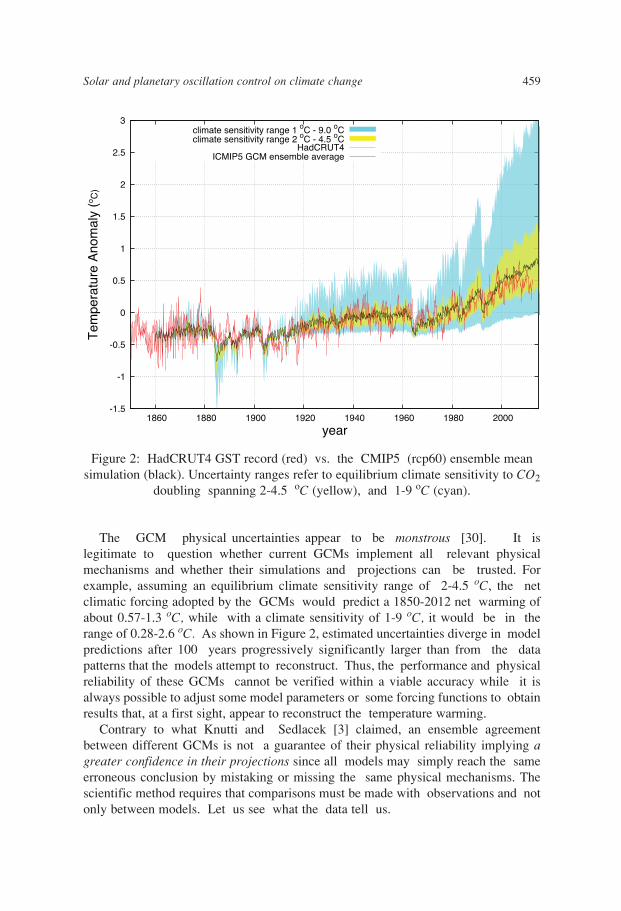
For example, Figure 3B shows for Central England the HadCET instrumentaltemperature record since ~1700 AD [48] and a proxy temperature reconstruction by Lamb[49] since ~900 AD. The shape clearly contradicts Mann’s hockey-stick GST: theimpression is that the warming trending observed since 1700 has been mostly due to aquasi-millennial natural oscillation driven by solar activity shown in Figure 3A [50]. Infact, Lamb’s curve suggests that in England the MWP was as warm as, or even warmerthan current temperatures. However, findings such as Lamb-like reconstructions weredismissed [35]. For example, Jones et al. [51] claimed that Lamb’s graph was notrepresentative of global conditions and that the techniques employed by Lamb were


6 http://www.ipcc.ch/ipccreports/far/wg_I/ipcc_far_wg_I_chapter_07.pdf7 http://www.grida.no/climate/ipcc_tar/vol4/english/pdf/wg1ts.pdf

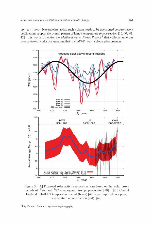
not very robust. Nevertheless, today such a claim needs to be questioned because recentpublications support the overall pattern of lamb’s temperature reconstruction [16, 40, 41,42]. It is worth to mention the Medieval Warm Period Project 8 that collects numerouspeer reviewed works documenting that the MWP was a global phenomenon.


8 http://www.co2science.org/data/mwp/mwpp.php

Figure 3: [A] Proposed solar activity reconstructions based on the solar proxyrecords of 10Be and 14C cosmogenic isotope production [50]. [B] CentralEngland: HadCET temperature record (black) [48] superimposed on a proxy

temperature reconstruction (red) [49].

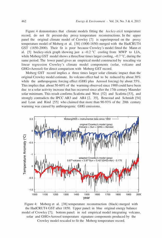
Figure 4 demonstrates that climate models fitting the hockey-stick temperaturerecord, do not fit present-day proxy temperature reconstructions. In the upperpanel the original climate model of Crowley [7] is superimposed on the proxytemperature model of Moberg et al. [38] (1000-1850) merged with the HadCRUT4GST (1850-2000). Their fit is poor because Crowley’s model fitted the Mann etal. [5] hockey-stick graph showing just a ~0.2 oC cooling from MWP to LIA,while Moberg GST model shows a three/four times larger cooling, ~0.7 oC, during thesame period. The lower panel gives an empirical model constructed by rescaling vialinear regression Crowley’s climate model components (solar, volcano andGHG+Aerosol) for direct comparison with Moberg GST record.

Moberg GST record implies a three times larger solar climatic impact than theoriginal Crowley model estimate. Its volcano effect had to be reduced by about 30%while the anthropogenic forcing effect (GHG plus Aerosol forcing) by about 55%.This implies that about 50-60% of the warming observed since 1900 could have beendue to a solar activity increase that has occurred since after the 17th century Maundersolar minimum. This result confirms Scafetta and West [52] and Scafetta [53], andstrongly contradicts the IPCC AR3 and AR4 [2, 35], Benestad and Schmidt [54]and Lean and Rind [55] who claimed that more than 90-93% of the 20th centurywarming was caused by anthropogenic GHG emissions.


Figure 4: Moberg et al. [38] temperature reconstruction (black) merged withthe HadCRUT4 GST after 1850. Upper panel: in blue original energy balance

model of Crowley [7]; bottom panel: in red empirical model integrating volcano,solar and GHG+Aerosol temperature signature components produced by the

Crowley model rescaled to fit the Moberg temperature record.

Thus, the energy balance model of Crowley [7] is unable to reproduce the empiri–cally determined solar signature evident in modern paleoclimatic GST reconstructions,and considerably overestimates the anthropogenic component. Today, the problem iseven more significant because the most recent GCMs (the CMIP5) use a solarforcing based on the total solar irradiance (TSI) reconstruction of Lean [56], whichshows a 50% smaller secular and millennial solar variability than the solar modelused by Crowley, which used the model by Bard et al. [50] rescaled on an earlier TSImodel by Lean et al. [57]. Therefore, or current GCMs use severely wrong TSI forcing(see Section 9), or they miss other solar related forcing mechanisms (e.g. chemical-based UV irradiance-related forcing of the stratospheric temperatures and a solarwind/cosmic ray forcing of the cloud systems [46]), or both.

Had in 2000 the current paleoclimatic temperature reconstructions been available,Crowley and other scientists of the time would have probably had a significantlylower confidence in the overall ability of climate models to simulate temperaturevariability, and would not have thought that the science was sufficiently settled.Very likely, those scientists would have concluded that important climate-changemechanisms were still unknown, and needed to be researched before they could beimplemented to make reliable climate models.

Today, the AGWT consensus appears to be an accident of history promotedsince 2001 by the discredited hockey-stick GST records and by the IPCC in a quitequestionable way [58, 59] and by numerous scientific organizations, such as thosethat in 2005 signed the Joint Science Academies statement (2005),9 that hastilyadvocated AGWT despite the scientific complexity of the climate system and thelarge known uncertainties demanded prudence. During the last decade there has beenalso a politically motivated consensus seeking process [60], which is inconclusive inquestions of science,10 that has likely interfered with the acquisition andinterpretation of evidences by discriminating opinions critical of the AGWT atmajor science journals [61]. This had also the effect to generate a serious tensionbetween the AGWT advocates [62] and the critical voices. However, becausenumerous evidences contradict the hockey-stick GST graph used since 2001 by theIPCC to promote the AGWT and the GST stopped to rise 15 years ago contraryto all GCM predictions [10] (Fig. 1), today a careful investigation on the climatechange attribution problem is necessary and legitimate.

4. DECADAL AND MULTIDECADAL CLIMATIC OSCILLATIONS ARESYNCHRONOUS TO MAJOR ASTRONOMICAL CYCLESGeophysical systems are characterized by oscillations at multiple time scales froma few hours to hundred thousands and millions of years [65]. Quasi decadal,bidecadal, 60 year , 80-90 year , 115 year , 1000 year and other oscillations are foundin global and regional temperature records, in the Atlantic MultidecadalOscillation (AMO), North Atlantic Oscillation (NAO) and Pacific DecadalOscillation (PDO), in global sea level rise indexes, monsoon records, and similaroscillations are found also in solar proxy records and in historical aurora records


9 http://nationalacademies.org/onpi/06072005.pdf10 It is worth reminding the famous quote attributed to Galileo Galilei: “In questions of science, theauthority of a thousand is not worth the humble reasoning of a single individual.”

covering centuries and millennia [e.g.: 8, 9, 11, 43, 45, 47, 67, 68, 69, 70, 71,72, 73, 74, 75, 76, 77, 78, 79, 80, 81, 82, 83, 84, 85, 86].

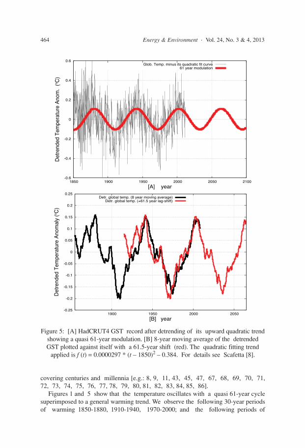
Figures 1 and 5 show that the temperature oscillates with a quasi 61-year cyclesuperimposed to a general warming trend. We observe the following 30-year periodsof warming 1850-1880, 1910-1940, 1970-2000; and the following periods of


Figure 5: [A] HadCRUT4 GST record after detrending of its upward quadratic trendshowing a quasi 61-year modulation. [B] 8-year moving average of the detrendedGST plotted against itself with a 61.5-year shift (red). The quadratic fitting trend

applied is f (t) = 0.0000297 * (t – 1850)2 – 0.384. For details see Scafetta [8].

cooling 1880-1910, 1940-1970, 2000-2030(?). By detrending the long-termwarming trend,11 the quasi 61-year oscillation can be highlighted, as shown inFigure 5 [8], where an almost perfect match between the 1880-1940 and 1940-2000GST periods emerges.

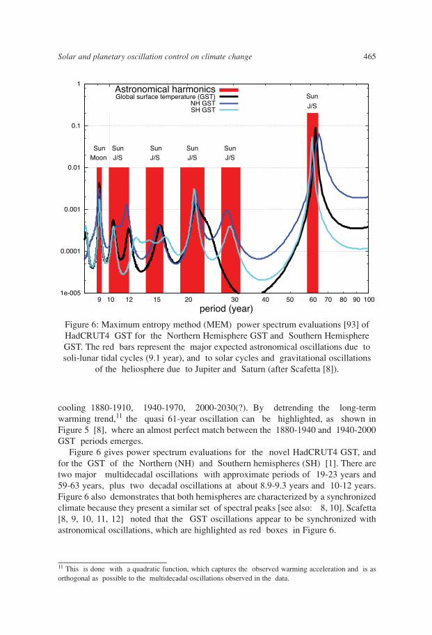
Figure 6 gives power spectrum evaluations for the novel HadCRUT4 GST, andfor the GST of the Northern (NH) and Southern hemispheres (SH) [1]. There aretwo major multidecadal oscillations with approximate periods of 19-23 years and59-63 years, plus two decadal oscillations at about 8.9-9.3 years and 10-12 years.Figure 6 also demonstrates that both hemispheres are characterized by a synchronizedclimate because they present a similar set of spectral peaks [see also: 8, 10]. Scafetta[8, 9, 10, 11, 12] noted that the GST oscillations appear to be synchronized withastronomical oscillations, which are highlighted as red boxes in Figure 6.


Figure 6: Maximum entropy method (MEM) power spectrum evaluations [93] ofHadCRUT4 GST for the Northern Hemisphere GST and Southern HemisphereGST. The red bars represent the major expected astronomical oscillations due tosoli-lunar tidal cycles (9.1 year), and to solar cycles and gravitational oscillations

of the heliosphere due to Jupiter and Saturn (after Scafetta [8]).

11 This is done with a quadratic function, which captures the observed warming acceleration and is asorthogonal as possible to the multidecadal oscillations observed in the data.

The 9.1 year oscillation probably relates to a major soli-lunar gravitational tidalcycle [8, 10, 66]. In fact, the lunar nodes complete a revolution in 18.6 years, andthe Saros soli-lunar eclipse cycle completes a revolution in 18 years and 11 days.These two cycles induce 9.3 year and 9.015 year tidal oscillations correspondingrespectively to Sun-Earth-Moon and Sun-Moon-Earth tidal configurations. Moreover,the lunar apsidal precession completes one rotation in 8.85 years causing acorresponding lunar tidal cycle. Thus, there are three interfering major tidal cyclesclustered between 8.85 year and 9.3 year periods, which generate a major oscillationwith an average period of about 9.06 years. Scafetta [10, supplement pp. 35-36]showed that in 1997-1998 and 2006-2007 eclipses occurred close to the March andSeptember equinoxes, that is when the soli-lunar spring tidal bulge peaks on theequator, having the strongest torquing effect on the ocean. Filtering methodologiesshowed the ~9.1 year GST cycle to peak in 1997-1998 and 2006-2007 as expected[10]. The Moon also causes an 18.6 year nutation cycle of the Earth’s axis, whichmay contribute to an 18.6 year climate oscillation [70]. This 18.6 year oscillationpresumably interferes with the two bi-decadal cycles of solar/planetary origin(discussed below), thus contributing to modulate a bidecadal cycle with an averageperiod varying between 18 and 23 years. Other long soli-lunar tidal oscillations mayexist. The solar system is also characterized by a set of natural harmonicsassociated with solar cycles (e.g. the ~11-year Schwabe sunspot cycle and the ~22-year Hale magnetic cycle [73]) and planetary harmonics: see Section 7.

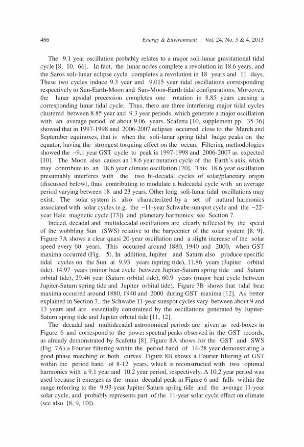
Indeed, decadal and multidecadal oscillations are clearly reflected by the speedof the wobbling Sun (SWS) relative to the barycenter of the solar system [8, 9].Figure 7A shows a clear quasi 20-year oscillation and a slight increase of the solarspeed every 60 years. This occurred around 1880, 1940 and 2000, when GSTmaxima occurred (Fig. 5). In addition, Jupiter and Saturn also produce specifictidal cycles on the Sun at 9.93 years (spring tide), 11.86 years (Jupiter orbitaltide), 14.97 years (minor beat cycle between Jupiter-Saturn spring tide and Saturnorbital tide), 29.46 year (Saturn orbital tide), 60.9 years (major beat cycle betweenJupiter-Saturn spring tide and Jupiter orbital tide). Figure 7B shows that tidal beatmaxima occurred around 1880, 1940 and 2000 during GST maxima [12]. As betterexplained in Section 7, the Schwabe 11-year sunspot cycles vary between about 9 and13 years and are essentially constrained by the oscillations generated by Jupiter-Saturn spring tide and Jupiter orbital tide [11, 12].

The decadal and multidecadal astronomical periods are given as red-boxes inFigure 6 and correspond to the power spectral peaks observed in the GST records,as already demonstrated by Scafetta [8]. Figure 8A shows for the GST and SWS(Fig. 7A) a Fourier filtering within the period band of 14-28 year demonstrating agood phase matching of both curves. Figure 8B shows a Fourier filtering of GSTwithin the period band of 8-12 years, which is reconstructed with two optimalharmonics with a 9.1 year and 10.2 year period, respectively. A 10.2 year period wasused because it emerges as the main decadal peak in Figure 6 and falls within therange referring to the 9.93-year Jupiter-Saturn spring tide and the average 11-yearsolar cycle, and probably represents part of the 11-year solar cycle effect on climate(see also [8, 9, 10]).


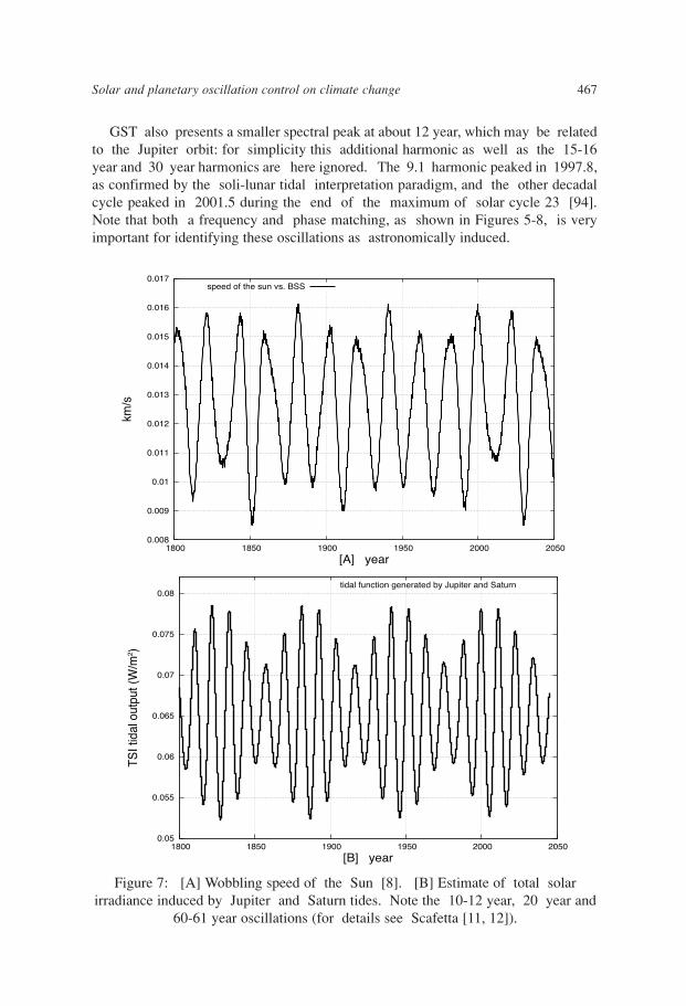
GST also presents a smaller spectral peak at about 12 year, which may be relatedto the Jupiter orbit: for simplicity this additional harmonic as well as the 15-16year and 30 year harmonics are here ignored. The 9.1 harmonic peaked in 1997.8,as confirmed by the soli-lunar tidal interpretation paradigm, and the other decadalcycle peaked in 2001.5 during the end of the maximum of solar cycle 23 [94].Note that both a frequency and phase matching, as shown in Figures 5-8, is veryimportant for identifying these oscillations as astronomically induced.


Figure 7: [A] Wobbling speed of the Sun [8]. [B] Estimate of total solarirradiance induced by Jupiter and Saturn tides. Note the 10-12 year, 20 year and

60-61 year oscillations (for details see Scafetta [11, 12]).

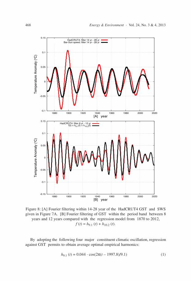
By adopting the following four major constituent climatic oscillation, regressionagainst GST permits to obtain average optimal empirical harmonics:

h9.1 (t) = 0.044 · cos(2π(t – 1997.8)/9.1) (1)


Figure 8: [A] Fourier filtering within 14-28 year of the HadCRUT4 GST and SWSgiven in Figure 7A. [B] Fourier filtering of GST within the period band between 8

years and 12 years compared with the regression model from 1870 to 2012,f (t) = h9.1 (t) + h10.2 (t).

h10.2 (t) = 0.030 · cos(2π(t – 2001.5)/10.2) (2)

h21 (t) = 0.051 · cos(2π(t – 2004.7)/21) (3)

h61 (t) = 0.107 · cos(2π(t – 2003.14)/61) (4)

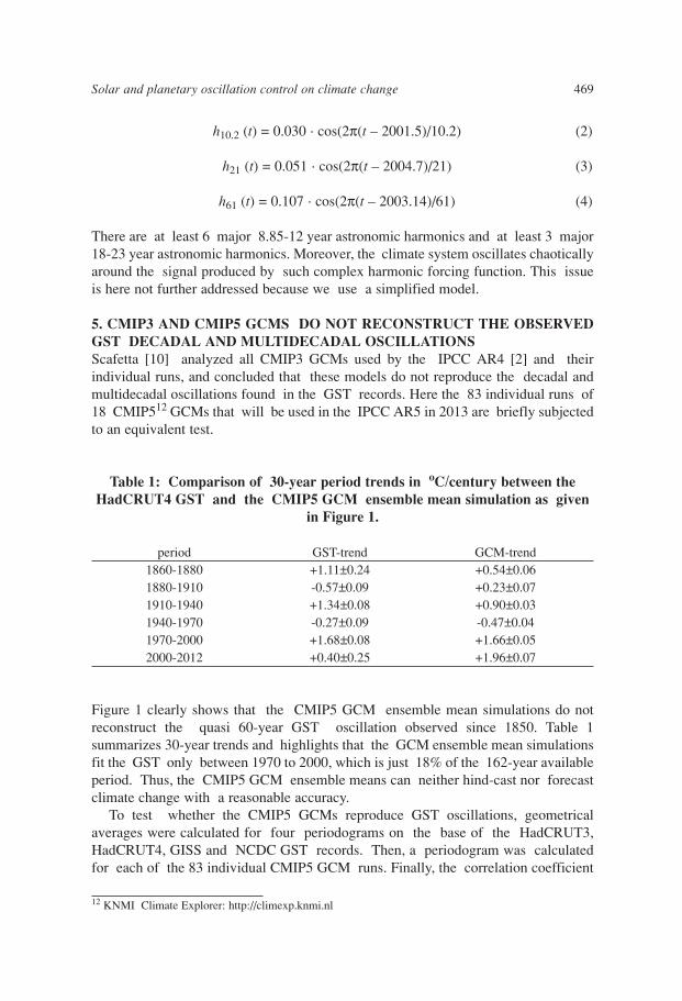
There are at least 6 major 8.85-12 year astronomic harmonics and at least 3 major18-23 year astronomic harmonics. Moreover, the climate system oscillates chaoticallyaround the signal produced by such complex harmonic forcing function. This issueis here not further addressed because we use a simplified model.

5. CMIP3 AND CMIP5 GCMS DO NOT RECONSTRUCT THE OBSERVEDGST DECADAL AND MULTIDECADAL OSCILLATIONSScafetta [10] analyzed all CMIP3 GCMs used by the IPCC AR4 [2] and theirindividual runs, and concluded that these models do not reproduce the decadal andmultidecadal oscillations found in the GST records. Here the 83 individual runs of18 CMIP512 GCMs that will be used in the IPCC AR5 in 2013 are briefly subjectedto an equivalent test.

Table 1: Comparison of 30-year period trends in oC/century between theHadCRUT4 GST and the CMIP5 GCM ensemble mean simulation as given

in Figure 1.

period GST-trend GCM-trend1860-1880 +1.11±0.24 +0.54±0.061880-1910 -0.57±0.09 +0.23±0.071910-1940 +1.34±0.08 +0.90±0.031940-1970 -0.27±0.09 -0.47±0.041970-2000 +1.68±0.08 +1.66±0.052000-2012 +0.40±0.25 +1.96±0.07

Figure 1 clearly shows that the CMIP5 GCM ensemble mean simulations do notreconstruct the quasi 60-year GST oscillation observed since 1850. Table 1summarizes 30-year trends and highlights that the GCM ensemble mean simulationsfit the GST only between 1970 to 2000, which is just 18% of the 162-year availableperiod. Thus, the CMIP5 GCM ensemble means can neither hind-cast nor forecastclimate change with a reasonable accuracy.

To test whether the CMIP5 GCMs reproduce GST oscillations, geometricalaverages were calculated for four periodograms on the base of the HadCRUT3,HadCRUT4, GISS and NCDC GST records. Then, a periodogram was calculatedfor each of the 83 individual CMIP5 GCM runs. Finally, the correlation coefficient


12 KNMI Climate Explorer: http://climexp.knmi.nl

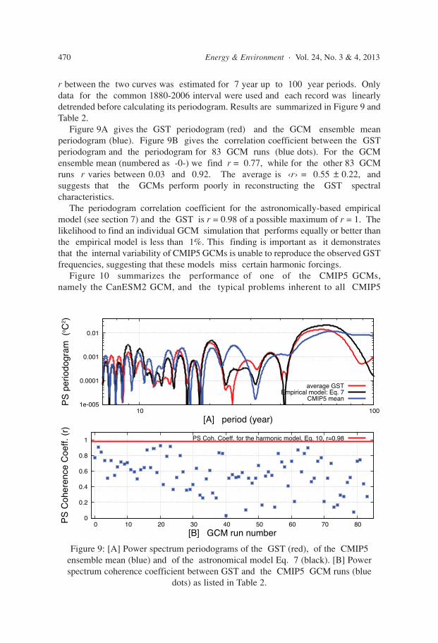
r between the two curves was estimated for 7 year up to 100 year periods. Onlydata for the common 1880-2006 interval were used and each record was linearlydetrended before calculating its periodogram. Results are summarized in Figure 9 andTable 2.

Figure 9A gives the GST periodogram (red) and the GCM ensemble meanperiodogram (blue). Figure 9B gives the correlation coefficient between the GSTperiodogram and the periodogram for 83 GCM runs (blue dots). For the GCMensemble mean (numbered as -0-) we find r = 0.77, while for the other 83 GCMruns r varies between 0.03 and 0.92. The average is ‹r› = 0.55 ± 0.22, andsuggests that the GCMs perform poorly in reconstructing the GST spectralcharacteristics.

The periodogram correlation coefficient for the astronomically-based empiricalmodel (see section 7) and the GST is r = 0.98 of a possible maximum of r = 1. Thelikelihood to find an individual GCM simulation that performs equally or better thanthe empirical model is less than 1%. This finding is important as it demonstratesthat the internal variability of CMIP5 GCMs is unable to reproduce the observed GSTfrequencies, suggesting that these models miss certain harmonic forcings.

Figure 10 summarizes the performance of one of the CMIP5 GCMs,namely the CanESM2 GCM, and the typical problems inherent to all CMIP5


Figure 9: [A] Power spectrum periodograms of the GST (red), of the CMIP5ensemble mean (blue) and of the astronomical model Eq. 7 (black). [B] Powerspectrum coherence coefficient between GST and the CMIP5 GCM runs (blue

dots) as listed in Table 2.

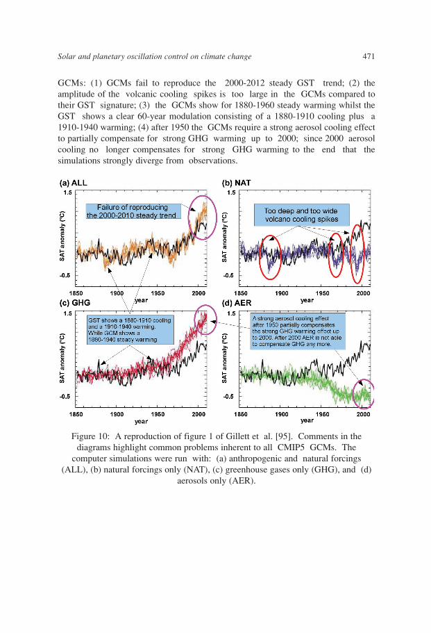
GCMs: (1) GCMs fail to reproduce the 2000-2012 steady GST trend; (2) theamplitude of the volcanic cooling spikes is too large in the GCMs compared totheir GST signature; (3) the GCMs show for 1880-1960 steady warming whilst theGST shows a clear 60-year modulation consisting of a 1880-1910 cooling plus a1910-1940 warming; (4) after 1950 the GCMs require a strong aerosol cooling effectto partially compensate for strong GHG warming up to 2000; since 2000 aerosolcooling no longer compensates for strong GHG warming to the end that thesimulations strongly diverge from observations.


Figure 10: A reproduction of figure 1 of Gillett et al. [95]. Comments in thediagrams highlight common problems inherent to all CMIP5 GCMs. The

computer simulations were run with: (a) anthropogenic and natural forcings(ALL), (b) natural forcings only (NAT), (c) greenhouse gases only (GHG), and (d)

aerosols only (AER).

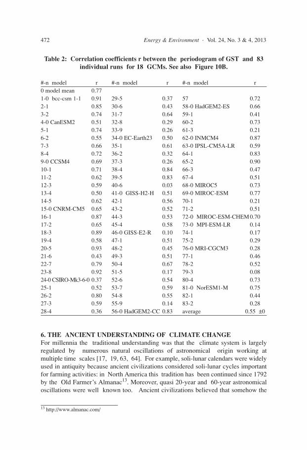
Table 2: Correlation coefficients r between the periodogram of GST and 83individual runs for 18 GCMs. See also Figure 10B.

#-n model r #-n model r #-n model r0 model mean 0.771-0 bcc-csm 1-1 0.91 29-5 0.37 57 0.722-1 0.85 30-6 0.43 58-0 HadGEM2-ES 0.663-2 0.74 31-7 0.64 59-1 0.414-0 CanESM2 0.51 32-8 0.29 60-2 0.735-1 0.74 33-9 0.26 61-3 0.216-2 0.55 34-0 EC-Earth23 0.50 62-0 INMCM4 0.877-3 0.66 35-1 0.61 63-0 IPSL-CM5A-LR 0.598-4 0.72 36-2 0.32 64-1 0.839-0 CCSM4 0.69 37-3 0.26 65-2 0.9010-1 0.71 38-4 0.84 66-3 0.4711-2 0.62 39-5 0.83 67-4 0.5112-3 0.59 40-6 0.03 68-0 MIROC5 0.7313-4 0.50 41-0 GISS-H2-H 0.51 69-0 MIROC-ESM 0.7714-5 0.62 42-1 0.56 70-1 0.2115-0 CNRM-CM5 0.65 43-2 0.52 71-2 0.5116-1 0.87 44-3 0.53 72-0 MIROC-ESM-CHEM 0.7017-2 0.65 45-4 0.58 73-0 MPI-ESM-LR 0.1418-3 0.89 46-0 GISS-E2-R 0.10 74-1 0.1719-4 0.58 47-1 0.51 75-2 0.2920-5 0.93 48-2 0.45 76-0 MRI-CGCM3 0.2821-6 0.43 49-3 0.51 77-1 0.4622-7 0.79 50-4 0.67 78-2 0.5223-8 0.92 51-5 0.17 79-3 0.0824-0 CSIRO-Mk3-6-0 0.37 52-6 0.54 80-4 0.7325-1 0.52 53-7 0.59 81-0 NorESM1-M 0.7526-2 0.80 54-8 0.55 82-1 0.4427-3 0.59 55-9 0.14 83-2 0.2828-4 0.36 56-0 HadGEM2-CC 0.83 average 0.55 ±0

6. THE ANCIENT UNDERSTANDING OF CLIMATE CHANGEFor millennia the traditional understanding was that the climate system is largelyregulated by numerous natural oscillations of astronomical origin working atmultiple time scales [17, 19, 63, 64]. For example, soli-lunar calendars were widelyused in antiquity because ancient civilizations considered soli-lunar cycles importantfor farming activities: in North America this tradition has been continued since 1792by the Old Farmer’s Almanac13. Moreover, quasi 20-year and 60-year astronomicaloscillations were well known too. Ancient civilizations believed that somehow the


13 http://www.almanac.com/

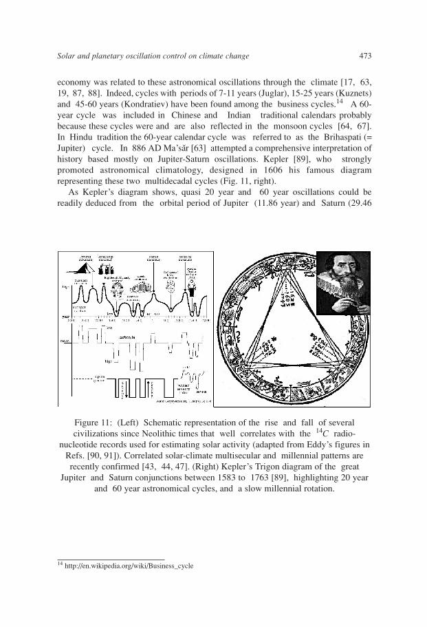
economy was related to these astronomical oscillations through the climate [17, 63,19, 87, 88]. Indeed, cycles with periods of 7-11 years (Juglar), 15-25 years (Kuznets)and 45-60 years (Kondratiev) have been found among the business cycles.14 A 60-year cycle was included in Chinese and Indian traditional calendars probablybecause these cycles were and are also reflected in the monsoon cycles [64, 67].In Hindu tradition the 60-year calendar cycle was referred to as the Brihaspati (=Jupiter) cycle. In 886 AD Ma’sar [63] attempted a comprehensive interpretation ofhistory based mostly on Jupiter-Saturn oscillations. Kepler [89], who stronglypromoted astronomical climatology, designed in 1606 his famous diagramrepresenting these two multidecadal cycles (Fig. 11, right).

As Kepler’s diagram shows, quasi 20 year and 60 year oscillations could bereadily deduced from the orbital period of Jupiter (11.86 year) and Saturn (29.46


14 http://en.wikipedia.org/wiki/Business_cycle

Figure 11: (Left) Schematic representation of the rise and fall of severalcivilizations since Neolithic times that well correlates with the 14C radio-

nucleotide records used for estimating solar activity (adapted from Eddy’s figures inRefs. [90, 91]). Correlated solar-climate multisecular and millennial patterns arerecently confirmed [43, 44, 47]. (Right) Kepler’s Trigon diagram of the great

Jupiter and Saturn conjunctions between 1583 to 1763 [89], highlighting 20 yearand 60 year astronomical cycles, and a slow millennial rotation.

year). The Jupiter-Saturn conjunction period is ~ 19.85 year, at ~242.57o of angle.Every ~60 years a conjunction Trigon completes with a ~7.7o rotation (Fig. 7).The full astronomical configuration repeats every ~900-960 years using the siderealorbital periods of the planets, as Ma’sar [63] observed following Ptolemy, or every~800 years using the tropical orbital periods, as Kepler [89] observed. In bothcases, the slow rotation of the Trigon convinced ancient civilizations of a quasi-millennia astronomical cycle that could be approximately correlated with a quasi-millennia cycle commonly observed in historical chronologies, as revealed by the riseand fall of civilizations. These events were likely driven by climatic variations (Fig.11, left) [90, 91].

Indeed, in 1345 AD a Jupiter-Saturn conjunction occurred in the zodiac sign ofAquarius and was linked to the outbreak of the Black Death epidemic [88, pp.158-172]15. In 1606 Kepler [89] used a related argument to predict that Europeancivilization would have flourished again during the following four/five centuries,and Newton excluded the possibility of another civilization collapse before 2060AD16. Today, it is known that this quasi-millennial civilization cycle is also reflectedin the 14C and 10Be cosmo-nucleotide records, which are modulated by solar activity[43, 44, 47] (Fig. 11) suggesting a planet-sun-climate link.

However, since the 18th century a planetary influence on the climate, as well asthe ancient astrological planetary models were dismissed as superstitions becauseaccording Newton’s gravitational law the planets are too far from the Earth tohave any observable effect. Is there a solution to this curious mystery? Below amodern astronomical interpretation of the climate oscillations is given based on someof the author’s studies [8, 9, 11, 12, 86].

7. PLANETARY CONTROL ON SOLAR AND CLIMATE CHANGEOSCILLATIONS THROUGHOUT THE HOLOCENEIn the 19th century an important discovery was made: the Sun oscillates withan apparent 11-year periodicity. In 1859 Wolf [96] postulated that the variations ofthe sunspot-frequency depends on the influences of Venus, Earth, Jupiter and Saturn.The theory of a planetary influence on solar activity was popular in the 19th andearlier 20th century [97, 98]. Although most solar physicists no longer favor thisconcept claiming that, e.g., planetary forces are too weak to influence solar activity(for a summary of objections see Ref. [11, 12]), Scafetta [11, 12] developed it furtherusing physics and data not yet available in the 19th century, found strong supportingempirical evidence for it and proposed a physical explanation.

Indeed, a number of recent studies since the 1970s noted correlations between thewobbling of the Sun around the center of mass of the solar system and climaticpatterns [99, 100, 101, 102, 103]. However, as the Sun is in free fall with respect tothe gravitational forces of the planets, its wobbling should not effect its activity.Scafetta [8, 9, 11, 12, 86] investigated this conundrum taking the following fouraspects into consideration:


15Traditional medieval astrology claimed that when the Trigon of the great conjunctions of Jupiter andSaturn occurred in the zodiac air sign of Aquarius kingdoms have been emptied and the earthdepopulated because of great cold, heavy frosts and thick clouds corrupting the air [88, pp. 172].16http://en.wikipedia.org/wiki/lsaac_Newton’s_occult_studies

1. Using Taylor’s theorem Scafetta [8] explained that even if the solar wobblingfunctions are not the direct physical cause of the observed effects, they canstill be used as proxies because they would present frequencies and geometricpatterns in common with the relevant physical functions even if the latter mayremain unknown.

2. The gravitational and electro-magnetic properties of the heliosphere may bemodulated by the reciprocal position and speed of the Jovian planets and ofthe Sun. Moreover, as solar wobbling is real relative to the Milky WayGalaxy, its velocity may modulate the incoming cosmic ray flux. Oscillatingelectro-magnetic properties of the heliosphere, of the solar wind and of theincoming cosmic ray flux probably cause climatic oscillations by means of acloud cover modulation [46, 104] and other electro-magnetic mechanisms.

3. The Jovian planets may periodically perturb the orbit of the Earth, causingspecific climatic oscillations as it happens with the multi-millenialMilankovic cycles [105] (eccentricity, 100,000-year cycle; axial tilt, 41,000-year cycle; precession, 23,000-year cycle), which are responsible forintermittent great glaciations. However, decadal-to-millennial scale orbitalperturbations appear to be too small (~ 1000 kilometers) to explain the decadal-to-millennial scale climatic oscillations by variations in the Earth-Sun distancebecause the Earth orbits the Sun and not the barycenter. Nevertheless, thishypothesis needs to be further investigated.

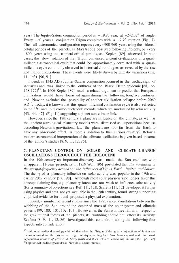
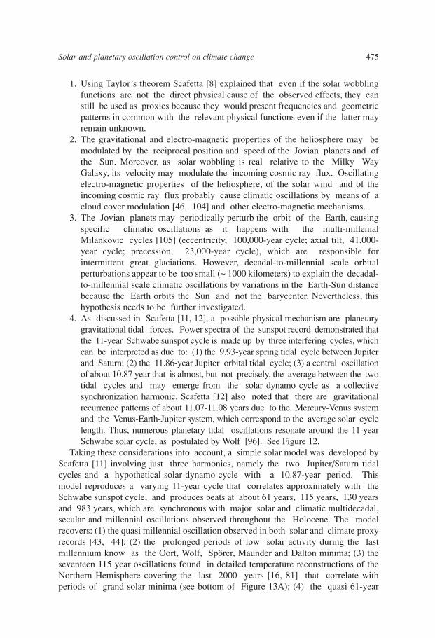
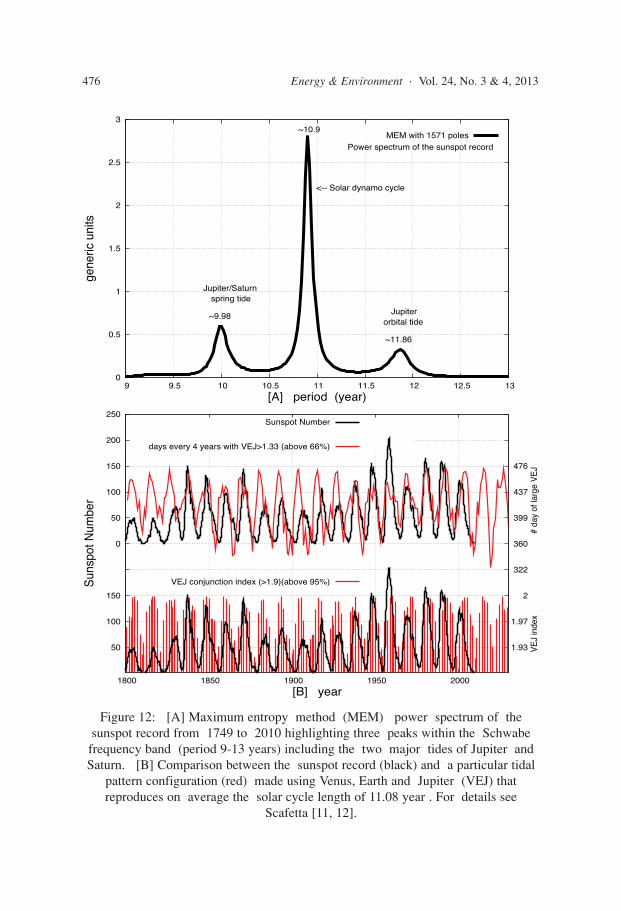
4. As discussed in Scafetta [11, 12], a possible physical mechanism are planetarygravitational tidal forces. Power spectra of the sunspot record demonstrated thatthe 11-year Schwabe sunspot cycle is made up by three interfering cycles, whichcan be interpreted as due to: (1) the 9.93-year spring tidal cycle between Jupiterand Saturn; (2) the 11.86-year Jupiter orbital tidal cycle; (3) a central oscillationof about 10.87 year that is almost, but not precisely, the average between the twotidal cycles and may emerge from the solar dynamo cycle as a collectivesynchronization harmonic. Scafetta [12] also noted that there are gravitationalrecurrence patterns of about 11.07-11.08 years due to the Mercury-Venus systemand the Venus-Earth-Jupiter system, which correspond to the average solar cyclelength. Thus, numerous planetary tidal oscillations resonate around the 11-yearSchwabe solar cycle, as postulated by Wolf [96]. See Figure 12.

Taking these considerations into account, a simple solar model was developed byScafetta [11] involving just three harmonics, namely the two Jupiter/Saturn tidalcycles and a hypothetical solar dynamo cycle with a 10.87-year period. Thismodel reproduces a varying 11-year cycle that correlates approximately with theSchwabe sunspot cycle, and produces beats at about 61 years, 115 years, 130 yearsand 983 years, which are synchronous with major solar and climatic multidecadal,secular and millennial oscillations observed throughout the Holocene. The modelrecovers: (1) the quasi millennial oscillation observed in both solar and climate proxyrecords [43, 44]; (2) the prolonged periods of low solar activity during the lastmillennium know as the Oort, Wolf, Spörer, Maunder and Dalton minima; (3) theseventeen 115 year oscillations found in detailed temperature reconstructions of theNorthern Hemisphere covering the last 2000 years [16, 81] that correlate withperiods of grand solar minima (see bottom of Figure 13A); (4) the quasi 61-year



Figure 12: [A] Maximum entropy method (MEM) power spectrum of thesunspot record from 1749 to 2010 highlighting three peaks within the Schwabefrequency band (period 9-13 years) including the two major tides of Jupiter andSaturn. [B] Comparison between the sunspot record (black) and a particular tidal

pattern configuration (red) made using Venus, Earth and Jupiter (VEJ) thatreproduces on average the solar cycle length of 11.08 year . For details see

Scafetta [11, 12].

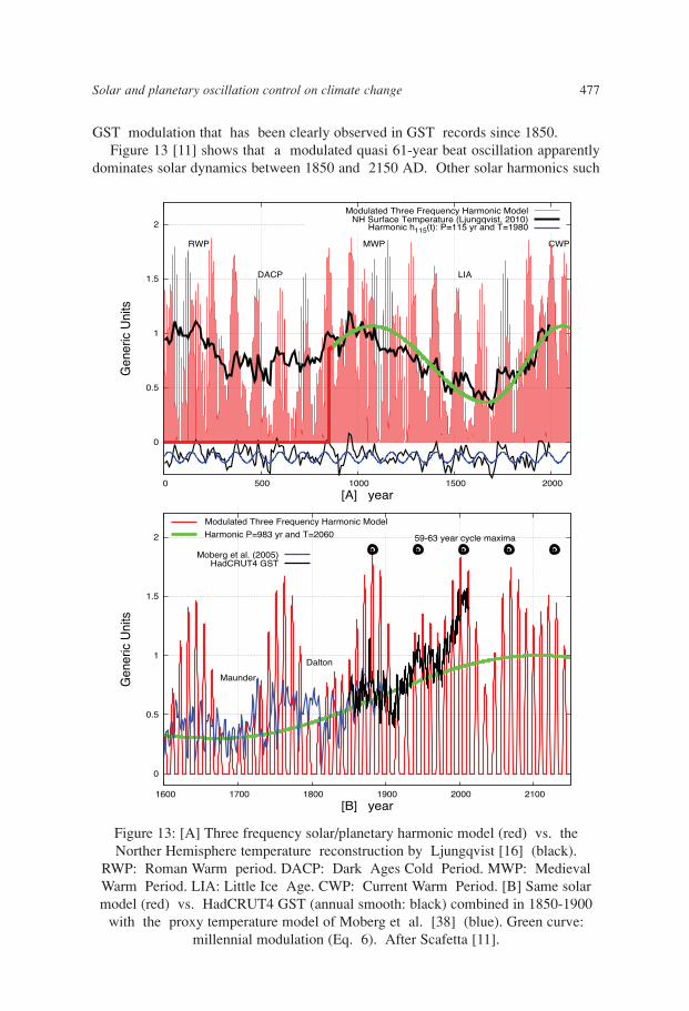
GST modulation that has been clearly observed in GST records since 1850.Figure 13 [11] shows that a modulated quasi 61-year beat oscillation apparently

dominates solar dynamics between 1850 and 2150 AD. Other solar harmonics such


Figure 13: [A] Three frequency solar/planetary harmonic model (red) vs. theNorther Hemisphere temperature reconstruction by Ljungqvist [16] (black).

RWP: Roman Warm period. DACP: Dark Ages Cold Period. MWP: MedievalWarm Period. LIA: Little Ice Age. CWP: Current Warm Period. [B] Same solarmodel (red) vs. HadCRUT4 GST (annual smooth: black) combined in 1850-1900

with the proxy temperature model of Moberg et al. [38] (blue). Green curve:millennial modulation (Eq. 6). After Scafetta [11].

as the ~87-year Gleissberg and the ~207-year de Vries solar cycles and other solarcycles can be readily discerned in the planetary harmonics [12, 86, 102]. In fact, the1/7 resonance of Jupiter and Uranus is about 85 years and other harmonics occurat 84-89 year periodicities [103, 86]; the beat resonance between the quasi 60-yearand the 85-year cycles is about 205 years. Solar variation is likely the result ofan internal complex collective synchronization dynamics [106] emerging fromnumerous gravitational and electro-magnetic harmonic forcings.

Scafetta [11] estimated that the 115-year cycle should peak in 1980 and the 983-year cycle in 2060. By using the paleoclimate temperature records given in Figures 3and 11A [16, 38], and by looking at the cooling between the Medieval Warm Period(MWP) ending around 1000 AD and the Little Ice Age (LIA) around 1670 AD, itcan be deduced that the amplitude of the 115-year cycle is about 0.1 ± 0.05 oC andthat the millennial cycle amplitude is about 0.7 ±0.3 oC . The millennial climatic cycleappears to have reached also a minimum around 1680: see also Humlum et al. [74].Therefore, the two cycles can be approximately represented as:

h115 (t) = 0.05 · cos(2π(t – 1980)/115) (5)

h983 (t) = 0.35 · cos(2π(t – 2060)/760) (6)

Eq. 6 uses the period of 760 years for simulating the skewness of the millennialclimatic cycle and should be valid from 1680 to 2060.

8. SUN AS AMPLIFIER OF PLANETARY ORBITAL OSCILLATIONSScafetta [12] proposed the following physical mechanism to explain how planetaryforces may modulate solar activity. Planetary tides on the Sun are extremely small,and therefore scientists were discouraged from believing that these regulate solaractivity. However, systems that generate energy can work as amplifiers and,evidently, the Sun is a powerful generator of energy. Since its nuclear fusion activityis regulated by gravity, the Sun may work as a huge amplifier of the smallplanetary gravitational tidal perturbations exerted on it.

Solar luminosity is related to solar gravity via the well-known Mass-Luminosityrelation: if the mass of the Sun increases, its internal gravity increases and makesmore work on its interior masses. Consequently, solar luminosity increases as: L/LS≈ (M/MS)4 [107]. For example, if the mass of all planets were added to the Sun, thetotal solar irradiance would increase by about 8 W/m2. Using an argument based onthe Mass-Luminosity relation, Scafetta [12] estimated that nuclear fusion couldgreatly amplify the weak gravitational tidal energetic signal dissipated inside the Sunby up to a 4 million factor. If this is so, planetary tides are able to trigger solarluminosity oscillations with a magnitude compatible with the observed TSIoscillations [94], and, consequently, may be able to modulate the solar dynamocycle. Alternative planetary mechanisms influencing the Sun may exist; see alsoWolff and Patrone [108] and Abreu et al. [102].


9. TOTAL SOLAR IRRADIANCE (TSI) UNCERTAINTY PROBLEMThe three-frequency solar model (Fig. 13) predicts, akin to the GST, that solaractivity increased from 1970 to 2000, reached a maximum around 2000, and willdecrease until the 2030s. However, the CMIP5 GCMs adopt a solar forcing deducedfrom Lean’s solar proxy models [56, 114] that show a flat TSI trend since 1955with a slight decrease since 1980. Also the CMIP3 GCMs used by the IPCC AR4[2] adopted Lean’s TSI models in an effort to show that during the last 40 years amore or less stable Sun could not be responsible for the observed warming afterthe1970s (see also Lockwood and Fröhlich [109]). This is a highly controversialissue that needs to be clarified.

It is claimed that Lean’s proxy models are supported by actual TSI observationsprovided by the PMOD satellite TSI composite [110, 111]. However, PMOD usedmodified TSI satellite records. For some unexplained reason, the scientificcommunity appears to ignore that not only have the experimental teams responsiblefor the TSI satellite data never validated these PMOD modifications of theirrecords, but explicitly stated that PMOD’s procedures are highly speculative and


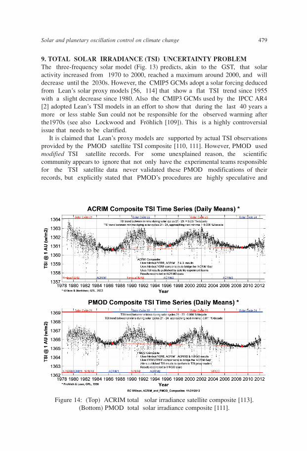
Figure 14: (Top) ACRIM total solar irradiance satellite composite [113].(Bottom) PMOD total solar irradiance composite [111].

physically incompatible with the experimental recording equipments [94, 112] (seethe Appendix). By contrast, the ACRIM TSI satellite composite [113] is based onTSI satellite data as published, and shows that TSI increased between 1980 and 2000and decreased thereafter. Figure 14 compares the ACRIM and PMOD TSIcomposites. With simple empirical thermal models Scafetta and West [52] andScafetta [53, 112] assessed the implication of adopting the ACRIM and PMOD TSIcomposites and showed that with the ACRIM record most of the climate changeobserved since the Maunder Minimum, including the 1970-2000 warming, can beattributed to variations in solar activity.

The controversy between the ACRIM and PMOD composites centers mainly onthe TSI trend during the so-called ACRIM-gap of 1989-1992. PMOD claims thatduring this period the Nimbus7/ERB TSI record, which is necessary to bridge theACRIM1 and ACRIM2 TSI records, must be shifted and inclined downward toproduce by 1992 a total downward shift of about 0.8-0.9 W/m2 [111, 112]. Thismodification of the Nimbus7/ERB TSI record results in a decreasing TSI trendduring 1989 to 1992 and causes in the PMOD TSI composite the 1996 TSIminimum to be almost at the same level as the 1986 TSI minimum [112]. On thecontrary, the ACRIM way of combining the TSI records without modifying themimplies that the 1996 minimum was about 0.5 W/m2 higher than the 1986 TSIminimum: this difference would be about 0.8-0.9 W/m2 by adopting the samecomposite PMOD merging methodology [112]. Thus, without PMOD’smodification, TSI clearly increased during 1980-2000, similar as the GST [52, 53].

Most arguments supporting the PMOD TSI composite are based on highlycontroversial proxy models such as Lean’s models and a few others [e.g.: 56, 110,116, 118], which agree with the flat PMOD TSI pattern partially employing circularreasoning. However, a correct scientific argument must focus on the ACRIM-gapdata to which the most important PMOD modifications are applied. Once this isdone Scafetta and Willson [94] showed that the model of Krivova et al. [116] isnot compatible with the PMOD modification of Nimbus7/ERB record. Krivova etal. [117] did not query this, but remarked that other proxy models, claimed to bemore accurate on short time scales, confirm the PMOD TSI composite. However,a direct comparison of the smoothed ACRIM and PMOD TSI composites and ofthe magnetogram-based SATIRE TSI model during the ACRIM-gap, as given byBall et al. [118, fig. 8], shows that, similar to ACRIM, from 1990 to 1992.5 alsoSATIRE trends upward from 1990 to 1992.5 (slope = 0.1 ± 0.03 W m–2 /year)approximately as in the original Nimbus7/ERB measurements. Also the ClimaxNeutron Monitor cosmic ray intensity count, which inversely correlates with solarmagnetic activity, decreases between 1989 and 1992 [112]. In general, the averagecosmic ray flux steadily decreased between 1965 and 1996 [46]. Therefore,preference should be given to the ACRIM TSI composite that is probably closerto reality than the PMOD TSI composite.

In addition, while the three-frequency solar model presents a maximum inthe 1940s that clearly correlates with a temperature maximum (Fig. 13), Lean’ssolar proxy models [56, 110] peak in 1960 similar to the sunspot number record.However, the solar maximum of the 1940s is supported by the TSI reconstruction


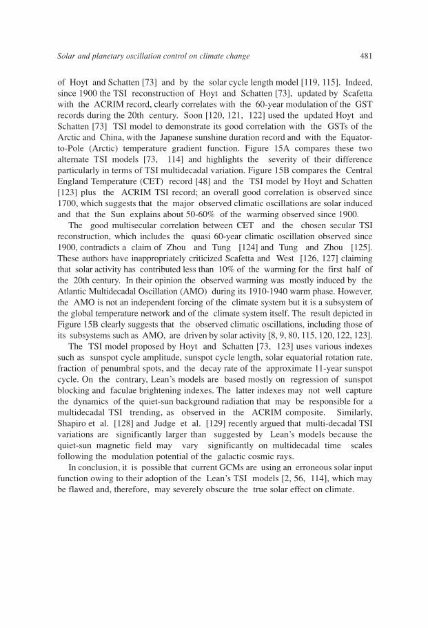
of Hoyt and Schatten [73] and by the solar cycle length model [119, 115]. Indeed,since 1900 the TSI reconstruction of Hoyt and Schatten [73], updated by Scafettawith the ACRIM record, clearly correlates with the 60-year modulation of the GSTrecords during the 20th century. Soon [120, 121, 122] used the updated Hoyt andSchatten [73] TSI model to demonstrate its good correlation with the GSTs of theArctic and China, with the Japanese sunshine duration record and with the Equator-to-Pole (Arctic) temperature gradient function. Figure 15A compares these twoalternate TSI models [73, 114] and highlights the severity of their differenceparticularly in terms of TSI multidecadal variation. Figure 15B compares the CentralEngland Temperature (CET) record [48] and the TSI model by Hoyt and Schatten[123] plus the ACRIM TSI record; an overall good correlation is observed since1700, which suggests that the major observed climatic oscillations are solar inducedand that the Sun explains about 50-60% of the warming observed since 1900.

The good multisecular correlation between CET and the chosen secular TSIreconstruction, which includes the quasi 60-year climatic oscillation observed since1900, contradicts a claim of Zhou and Tung [124] and Tung and Zhou [125].These authors have inappropriately criticized Scafetta and West [126, 127] claimingthat solar activity has contributed less than 10% of the warming for the first half ofthe 20th century. In their opinion the observed warming was mostly induced by theAtlantic Multidecadal Oscillation (AMO) during its 1910-1940 warm phase. However,the AMO is not an independent forcing of the climate system but it is a subsystem ofthe global temperature network and of the climate system itself. The result depicted inFigure 15B clearly suggests that the observed climatic oscillations, including those ofits subsystems such as AMO, are driven by solar activity [8, 9, 80, 115, 120, 122, 123].

The TSI model proposed by Hoyt and Schatten [73, 123] uses various indexessuch as sunspot cycle amplitude, sunspot cycle length, solar equatorial rotation rate,fraction of penumbral spots, and the decay rate of the approximate 11-year sunspotcycle. On the contrary, Lean’s models are based mostly on regression of sunspotblocking and faculae brightening indexes. The latter indexes may not well capturethe dynamics of the quiet-sun background radiation that may be responsible for amultidecadal TSI trending, as observed in the ACRIM composite. Similarly,Shapiro et al. [128] and Judge et al. [129] recently argued that multi-decadal TSIvariations are significantly larger than suggested by Lean’s models because thequiet-sun magnetic field may vary significantly on multidecadal time scalesfollowing the modulation potential of the galactic cosmic rays.

In conclusion, it is possible that current GCMs are using an erroneous solar inputfunction owing to their adoption of the Lean’s TSI models [2, 56, 114], which maybe flawed and, therefore, may severely obscure the true solar effect on climate.



Figure 15: [A] Total solar irradiance (TSI) reconstruction by Hoyt and Schatten[73, 123] updated with the ACRIM record [113] (since 1980) (red) vs. the

updated Lean’s model [56, 114] (blue) used as solar forcing function in the CMIP5GCMs adopted in the IPCC AR5 in 2013. [B] Comparison between the Central

England Temperature (black) Parker et al. [48] and the TSI model by Hoyt andSchatten [123] plus the ACRIM TSI record.

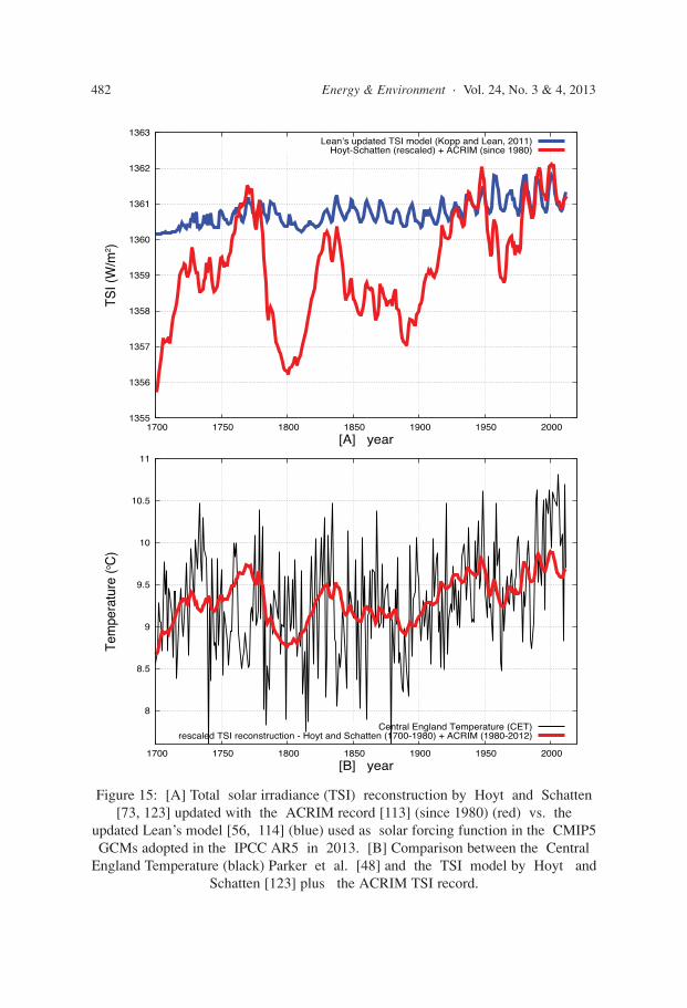
10. EMPIRICAL ASTRONOMICAL MODELThe six climatic harmonics synchronous with astronomic cycles at decadal to themillennial time scales are approximated by Eqs. 1-6. These harmonics describephenomenologically the natural climatic oscillations observed since 1850 and, asdemonstrated above and in Ref. [10], are not reproduced by the GCMs. Thesefunctions permit empirical modeling of natural variability at decadal to millennialtime scales. However, GST also depends on the chemical composition of theatmosphere that can be modified by anthropogenic emissions and volcano activity.

As discussed in the introduction, the IPCC AR4 [2] concluded that 100% of the~0.5-0.55 C o warming observed since 1970 can only be explained by anthropogenicforcing. However, its adopted GCMs fail to reproduce the natural harmonics suchas the 60-year oscillation (Fig. 5). Scafetta [10] argued that the failure of the GCMsto properly reproduce the 60-year oscillation, which contributed about 0.3 oC ofwarming between 1970 and 2000, caused the GCMs to overestimate the climaticeffect of anthropogenic forcing by about 50-60%. Zhou and Tung [124] reached asimilar conclusion by using the Atlantic Multidecadal Oscillation that shows a clear60-year oscillation [131, fig. 9B] without realizing that climatic oscillations such asAMO may be astronomical/solar induced. Even assuming that the anthropogenicforcing functions used in the GCMs are correct, the above arguments imply that theGCMs significantly overestimated the climate sensitivity to radiative forcing becausetheir output ought to be reduced to about a factor of 0.45. Such a reduction is inkeeping with modern paleoclimatic reconstructions (Fig. 4) and the calculations insection 3. The proposed correction provides a first approximation estimate of theclimatic effect of the anthropogenic plus volcano forcings, given that according theCMIP5 GCMs, the solar contribution to the secular GST trend is nearly insignificant(at best a few percent).

GST can be phenomenologically modeled with the following equation:

f (t) = h9.1 (t) + h10.2 (t) + h21 (t) + h61 (t) + h115 (t) + h983 (t) + MA,V (t), (7)

where the natural harmonic component of the climate system is reconstructed by thesix harmonics that are presumably induced by synchronized astronomical harmonicforcings. The function MA,V (t) = 0.45 · mGCM (t) is the output of the GCMensemble averages, mGCM (t), given in Figure 1, reduced to a 0.45 factor. In firstapproximation MA,V (t) would simulate the anthropogenic and the short-scale strongvolcano effects on climate under the assumption that the true equilibrium climatesensitivity to radiative forcing is 55% smaller than the one currently simulated bythe GCMs.

The empirical climate model of Eq. 7 may require additional harmonics to includethe effects of other minor oscillations and some additional nonlinear effect. Inparticular, Figure 13 indicates that the 61-year solar oscillation appears to be strongin 1850-2150, but too faint before 1850, while the 115-year oscillation appearsto be stronger before 1850, giving rise to the cold Maunder and Dalton periods.For simplicity, these corrections are ignored.



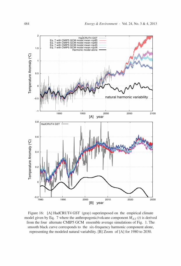
Figure 16: [A] HadCRUT4 GST (gray) superimposed on the empirical climatemodel given by Eq. 7 where the anthropogenic/volcano component MA,V (t) is derived

from the four alternate CMIP5 GCM ensemble average simulations of Fig. 1. Thesmooth black curve corresponds to the six-frequency harmonic component alone,representing the modeled natural variability. [B] Zoom of [A] for 1980 to 2030.

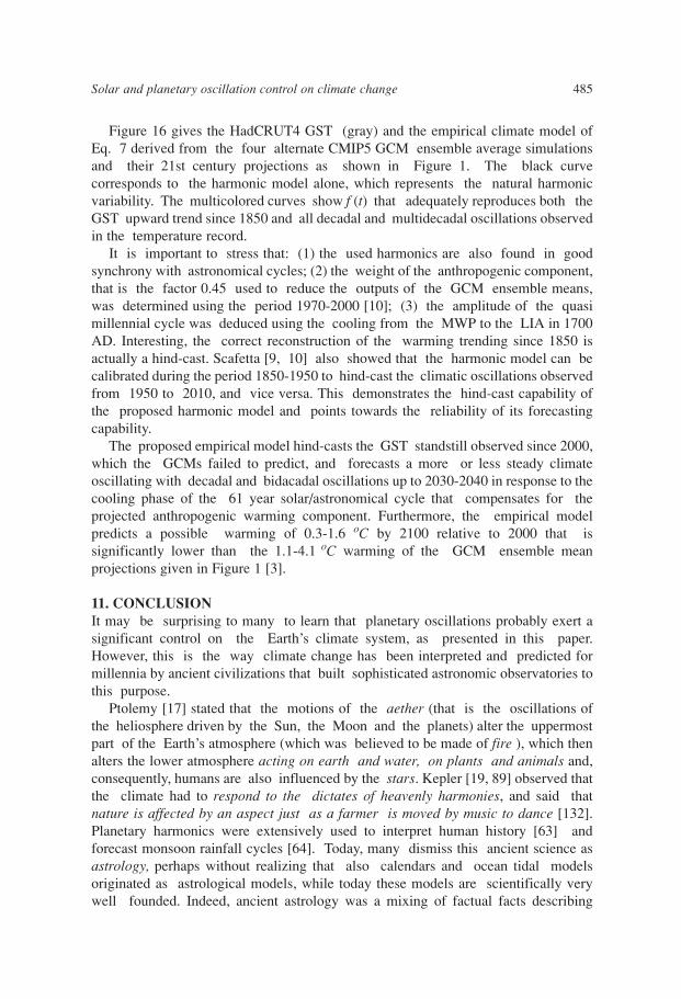
Figure 16 gives the HadCRUT4 GST (gray) and the empirical climate model ofEq. 7 derived from the four alternate CMIP5 GCM ensemble average simulationsand their 21st century projections as shown in Figure 1. The black curvecorresponds to the harmonic model alone, which represents the natural harmonicvariability. The multicolored curves show f (t) that adequately reproduces both theGST upward trend since 1850 and all decadal and multidecadal oscillations observedin the temperature record.

It is important to stress that: (1) the used harmonics are also found in goodsynchrony with astronomical cycles; (2) the weight of the anthropogenic component,that is the factor 0.45 used to reduce the outputs of the GCM ensemble means,was determined using the period 1970-2000 [10]; (3) the amplitude of the quasimillennial cycle was deduced using the cooling from the MWP to the LIA in 1700AD. Interesting, the correct reconstruction of the warming trending since 1850 isactually a hind-cast. Scafetta [9, 10] also showed that the harmonic model can becalibrated during the period 1850-1950 to hind-cast the climatic oscillations observedfrom 1950 to 2010, and vice versa. This demonstrates the hind-cast capability ofthe proposed harmonic model and points towards the reliability of its forecastingcapability.

The proposed empirical model hind-casts the GST standstill observed since 2000,which the GCMs failed to predict, and forecasts a more or less steady climateoscillating with decadal and bidacadal oscillations up to 2030-2040 in response to thecooling phase of the 61 year solar/astronomical cycle that compensates for theprojected anthropogenic warming component. Furthermore, the empirical modelpredicts a possible warming of 0.3-1.6 oC by 2100 relative to 2000 that issignificantly lower than the 1.1-4.1 oC warming of the GCM ensemble meanprojections given in Figure 1 [3].

11. CONCLUSIONIt may be surprising to many to learn that planetary oscillations probably exert asignificant control on the Earth’s climate system, as presented in this paper.However, this is the way climate change has been interpreted and predicted formillennia by ancient civilizations that built sophisticated astronomic observatories tothis purpose.

Ptolemy [17] stated that the motions of the aether (that is the oscillations ofthe heliosphere driven by the Sun, the Moon and the planets) alter the uppermostpart of the Earth’s atmosphere (which was believed to be made of fire ), which thenalters the lower atmosphere acting on earth and water, on plants and animals and,consequently, humans are also influenced by the stars. Kepler [19, 89] observed thatthe climate had to respond to the dictates of heavenly harmonies, and said thatnature is affected by an aspect just as a farmer is moved by music to dance [132].Planetary harmonics were extensively used to interpret human history [63] andforecast monsoon rainfall cycles [64]. Today, many dismiss this ancient science asastrology, perhaps without realizing that also calendars and ocean tidal modelsoriginated as astrological models, while today these models are scientifically verywell founded. Indeed, ancient astrology was a mixing of factual facts describing


astronomical-geophysical phenomena and superstitions and, by understanding this,Kepler warned to not throw out the baby with the bathwater [19, 133].

The GST clearly oscillates and increased since 1850. However, the GCMs usedby the IPCC, such as the CMIP3 in 2007 and the CMIP5 in 2013, are unable toreconstruct the observed GST decadal and multidecadal oscillations. The traditionaljustification for this failure has been attributed to an internal variability of the climatesystem that appears impossible to properly model due to uncertainties in the initialconditions and to the chaotic dynamics of the climate system itself.

The author [8, 9, 10, 11, 12] noted that the GST records are characterized byspecific frequency peaks corresponding to astronomical harmonics linked to soli-lunar tidal cycles, solar cycles and heliosphere oscillations in response to movementsof the planets, particularly of Jupiter and Saturn. Moreover, he proposed a physicalmodel that may explain how planetary tidal harmonics can modulate solar activity,and reconstructed the major known Holocene solar variations [11, 12] from thedecadal to the millennial scales. Figures 6, 9 and 13 show that the observed GSTand astronomic oscillations are well synchronized. Indeed, a planetary hypothesis ofsolar variation is reviving [134].

Empiric harmonic models based on these oscillations are able to reconstruct allobserved major decadal and multidecadal climate variations with a far greateraccuracy than any IPCC AGWT GCMs. A simple harmonic model based on aminimum of four astronomic oscillations with periods of about 9.1, 10-12, 19-22and 59-63 years can readily reconstruct and hind-cast all so-called GST hiatus periodsobserved since 1850. This contradicts Meehl et al. [22] that the observed GSToscillations are due to an unpredictable internal variability of the climate system.

The full GST record can be reconstructed by using two additional secular (~115years) and millennial (~983 years) astronomical harmonics plus a climate componentregulated by the chemical properties of the atmosphere (e.g. GHG and aerosols). TheGCM ensemble means can be used to estimate the effect of this component providedthat their output is reduced to a 0.45 factor. Thus, while the current GCMs producean average climate sensitivity to CO2 doubling to be around 3 oC, the real averagevalue of the climate sensitivity may be approximately 1.35 oC and may very likelyvary from 0.9 to 2.0 oC. The climate sensitivity may be lower, though, provided partof the GST warming of non-climatic origin, such as uncorrected urban heat island(UHI) effects [13, 14] or if the preindustrial GST millennial variability is foundlarger than what used in Eq. 7 [41]. This estimate of low equilibrium climatesensitivity to radiative forcing is compatible with the results of other studies [28, 29].

The empirical model given in Figure 16 implies that about 50-60% of the about0.8-0.85 oC warming observed since 1850 is due to a combination of naturaloscillations, including a quasi-millennial cycle that was in its warming phase since1700 AD. Since 1850 major quasi 20-year and 61-year cycles describe the GSTmultidecadal scales, and two decadal cycles of about 9.1 years and 10-11 yearscapture the decadal GST scale. Other minor oscillations of about 12, 15 and 30year period, also linked to astronomical oscillations (see Fig. 6) appear to be presentbut are ignored here. The proposed six-frequency empirical climate model, Eq. 7,outperforms all CMIP3 and CMIP5 GCM runs, and predicts under the same


emission scenarios a significantly lower warming for the 21st century ranging from0.3 oC to 1.6 oC , which is an upper limit.

The results of this analysis indicate that the GCMs do not yet include importantphysical mechanisms associated with natural oscillations of the climate system.Therefore, interpretations and predictions of climate change based on the currentGCMs, including the CMIP5 GCMs to be used in the IPCC AR5, is questionable.Mechanisms missing in the GCMs are probably linked to natural solar/astronomicaloscillations of the solar system that are a subject of further research. However,these oscillations can be already empirically modeled and, in first approximation,used for forecasting at least the harmonic component of the climate system.

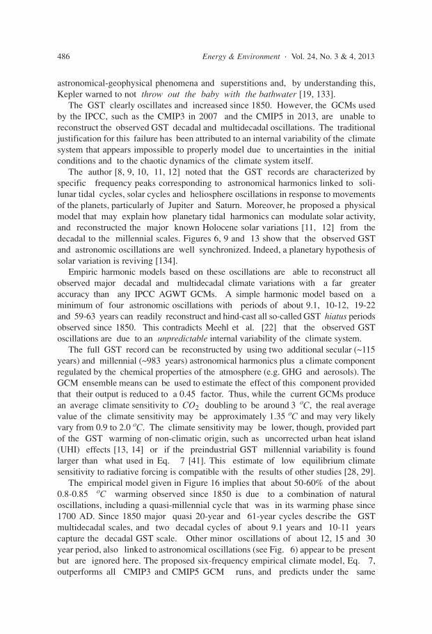
Figure 17 presents a qualitative diagram summarizing the network of the possiblephysical interaction between planetary harmonics, solar variability, soli-lunar tidalforcings, climate and environmental changes on our Earth. Taking into account aplanetary oscillation control of solar activity and lunar harmonics controlling director indirect natural climatic forcings, may make solar and climate change morepredictable.

12. ACKNOWLEDGMENTSThe author gratefully thanks Prof. Arthur Rörsch, Prof. Peter A. Ziegler andanonymous reviewers for detailed suggestions.


Figure 17: Network of the possible physical interaction between planetaryharmonics, solar variability and climate and environments changes on Planet Earth

(with permission adapted after Mörner [135]).

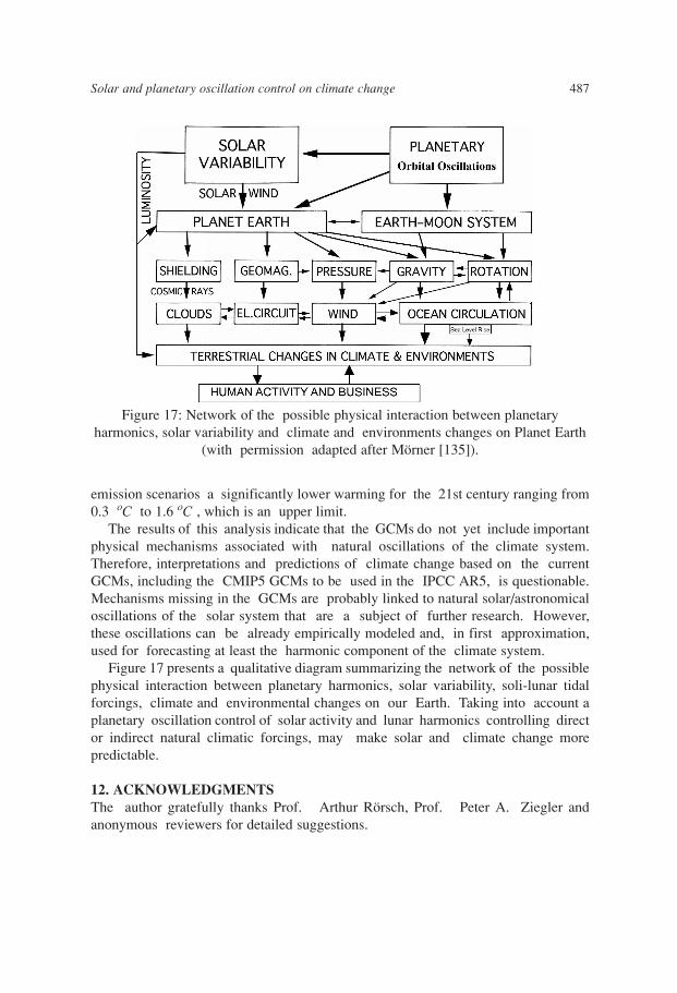
Appendix: Willson and Hoyt’s statements regarding the TSI satelliterecordsIn 2008 the author inquired with Dr. Willson, who heads the ACRIM satellite TSImeasurements, and Dr. Hoyt (the inventor of GSN Group Sunspot Numberindicator) who was in charge of the Nimbus7/ERB satellite measurements, abouttheir opinion regarding the theoretical modifications applied to their published TSIrecords by Dr. Fröhlich of the PMOD/WRC team. These modifications are crucialfor obtaining a TSI satellite composite record that does not show an increasing trendbetween 1980 and 2000 [110, 111], as shown in Figure 14. For detailed informationvisit ACRIM website17.

In the statements reproduced in Figure 18, Willson and Hoyt agree thatFröhlich’s modifications are, in their opinion, not justified because they are


17 http://acrim.com/TSI%20Monitoring.htm

Figure 18: Willson and Hoyt’s statements regarding the modificationsimplemented by Frohlich [110, 111] to the ACRIM and Nimbus 7 published

records.

inconsistent with the physical properties of the experimental instruments used for TSIsatellite measurements. Of course, these statements do not automatically imply thatFröhlich’s modifications are necessarily erroneous. However, it is clear that Willsonand Hoyt, who are the principal investigators of the experimental teams in charge ofthe TSI satellite records modified by Fröhlich, are convinced that the modificationof their TSI records are not justified and that the PMOD TSI satellite composite doesnot correspond to the actual TSI satellite measurements and does not properlydescribe the actual dynamic behavior of TSI from 1978 onward.

REFERENCES1. Morice, C. P., et al., 2012. Quantifying uncertainties in global and regional temperature

change using an ensemble of observational estimates: The Had– CRUT4 dataset.Journal Geophysical Research 117, D08101.

2. IPCC AR4. Climate Change 2007: The Physical Science Basis. Contribution of WorkingGroup I to the Fourth Assessment Report of the Intergovernmental Panel on ClimateChange. Cambridge, UK: Cambridge University Press; 2007.

3. Knutti, R., and J. Sedlá˘cek, 2012. Robustness and uncertainties in the new CMIP5climate model projections. Nature Climate Change. DOI: 10.1038/NCLIMATE1716

4. Knight J., et al., 2009. Do global temperature trends over the last decade falsifyclimate predictions? in State of the Climate in 2008”. Bulletin of the AmericanMeteorological Society 90, S1-S196.

5. Mann, M. E., R. S. Bradley, and M. K. Hughes, 1999. Northern hemispheretemperatures during the past millennium: Inferences, uncertainties, and limitations.Geophysical Research Letters, 26(6) 759-762.

6. Mann M. E., and P. D. Jones, 2003. Global surface temperature over the past twomillennia. Geophysical Research Letters 30, 1820-1824.

7. Crowley, T. J., 2000. Causes of Climate Change Over the Past 1000 Years. Science 289,270-277.

8. Scafetta, N., 2010. Empirical evidence for a celestial origin of the climate oscillationsand its implications. Journal of Atmospheric and Solar-Terrestrial Physics 72, 951-970.

9. Scafetta, N., 2012a. A shared frequency set between the historical mid-latitude aurorarecords and the global surface temperature. Journal of Atmospheric and Solar-TerrestrialPhysics 74, 145-163.

10. Scafetta, N., 2012b. Testing an astronomically based decadal-scale empirical harmonicclimate model versus the IPCC (2007) general circulation climate models. Journal ofAtmospheric and Solar-Terrestrial Physics 80, 124-137.

11. Scafetta, N., 2012c. Multi-scale harmonic model for solar and climate cyclicalvariation throughout the Holocene based on Jupiter-Saturn tidal frequencies plus the11-year solar dynamo cycle. Journal of Atmospheric and Solar- Terrestrial Physics 80,296-311.


12. Scafetta, N., 2012d. Does the Sun work as a nuclear fusion amplifier of planetary tidalforcing? A proposal for a physical mechanism based on the massluminosity relation.Journal of Atmospheric and Solar-Terrestrial Physics 81-82, 27-40.

13. McKitrick, R. R., and P. J. Michaels, 2007. Quantifying the influence of anthropogenicsurface processes and inhomogeneities on gridded global climate data. Journal ofGeophysical Research 112, D24S09.

14. McKitrick, R. R. and N. Nierenberg, 2010. Socioeconomic Patterns in Climate Data.Journal of Economic and Social Measurement 35, 149-175.

15. D’Arrigo, R., et al., 2008. On the ‘Divergence Problem’ in Northern Forests: A reviewof the tree-ring evidence and possible causes. Global and Planetary Change 60, 289-305.

16. Ljungqvist F. C., 2010. A new reconstruction of temperature variability in the extra-tropical Northern Hemisphere during the last two millennia. Geografiska AnnalerSeries A 92, 339-351.

17. Ptolemy, C., 2nd century. Tetrabiblos. Compiled and edited by F.E. Robbins, 1940.(Harvard University Press, Cambridge, MA).

18. Saint Bede, 725. The Reckoning of Time. Translated and Edited by F. Wallis, 1999.(Liverpool University Press).

19. Kepler, J., 1601. On the More Certain Fundamentals of Astrology. In: Brackenridge,J.B., and Rossi, M.A. (Eds.), Proceedings of the American Philosophical Society 123,85-116 (1979).

20. (Lord Kelvin) Thomson, W., 1881. The tide gauge, tidal harmonic analyzer, and tidepredictor. Proceedings of the Institution of Civil Engineers 65, 3-24.

21. Ehret, T., 2008. Old brass brains: mechanical prediction of tides. ACSM Bulletin 6,41-44.

22. Meehl G. A., et al., 2011. Model-based evidence of deep-ocean heat uptake duringsurface-temperature hiatus periods. Nature Climate Change 1, 360-364.

23. Kaufmann, R. K., et al., 2011. Reconciling anthropogenic climate change with observedtemperature 1998-2008. PNAS 108, 11790-11793.

24. Remer, L. A., et al., 2008. Global aerosol climatology from the MODIS satellitesensors. Journal of Geophysical Research 113, D14S07.

25. Kiehl, J. T., 2007. Twentieth century climate model response and climate sensitivity.Geophysical Research Letters 34, L22710.

26. Knutti, R., 2008. Why are climate models reproducing the observed global surfacewarming so well? Geophysical Research Letters 35, L18704.

27. Rahmstorf, S., 2008. Anthropogenic Climate Change: Revisiting the Facts. In GlobalWarming: Looking Beyond Kyoto. Ed. Zedillo, E. (Brookings Institution Press) p. 34-53.

28. Lindzen, R. S., and Y.-S. Choi, 2011. On the observational determination of climatesensitivity and its implications. Asia Pacific Journal of Atmospheric Science 47, 377-390.


29. Spencer, R. W., and W. D. Braswell, 2011. On the misdiagnosis of surface temperaturefeedbacks from variations in earth’s radiant energy balance. Remote Sensing 3,1603-1613.

30. Curry, J. A. and P. J. Webster, 2011. Climate Science and the Uncertainty Monster.Bulletin of the American Meteorological Society, 92, 1667-1682.

31. Guidoboni, E., A. Navarra and E. Boschi, 2011. The spiral of climate: civilizations ofthe mediterranean and climate change in history. (Bononia University Press, BolognaItaly).

32. IPCC FAR. Climate Change: Scientific Assessment. Contribution of Working GroupI to the First Assessment Report of the Intergovernmental Panel on ClimateChange. Cambridge, UK: Cambridge University Press, 1990.

33. Hegerl, G. C., et al., 2003. Detection of volcanic, solar and greenhouse gas signalsin paleo-reconstructions of Northern Hemispheric temperature. Geophysical ResearchLetters 30, 1242-1246.

34. Foukal, P., et al., 2006. Variations in solar luminosity and their effect on Earth’s climate.Nature 443, 161-166.

35. IPCC AR3. Climate Change 2001: The Scientific Basis. Contribution of Working GroupI to the Third Assessment Report of the Intergovernmental Panel on Climate Change.Cambridge, UK: Cambridge University Press, 2001.

36. Soon, W., and S. Baliunas, 2003. Proxy climatic and environmental changes of thepast 1000 years. Climate Research 23, 89-110.

37. McIntyre, S., and R. McKitrick, 2005. Hockey sticks, principal components, andspurious significance. Geophysical Research Letters 32, L03710.

38. Moberg, A., et al., 2005. Highly variable Northern Hemisphere temperaturesreconstructed from lowand high-resolution proxy data. Nature 433, 613-617.

39. Mann, M. E., et al., 2008. Proxy-based reconstructions of hemispheric and globalsurface temperature variations over the past two millennia. PNAS 105, 13252-13257.

40. Loehle, C., and J. H. Mc Culloch, 2008. Correction to: A 2000-year global temperaturereconstruction based on non-tree ring proxies. Energy & Environment 19, 93-100.

41. Christiansen, B., and F. C. Ljungqvist, 2012. The extra-tropical Northern Hemispheretemperature in the last two millennia: reconstructions of low-frequency variability.Climate of the Past 8, 765-786.

42. Esper, J., et al., 2012. Variability and extremes of northern Scandinavian summertemperatures over the past two millennia. Global and Planetary Change 88–89, 1-9.

43. Bond, G., et al., 2001. Persistent solar influence on North Atlantic climate during theHolocene. Science 294, 2130-2136.

44. Kerr, R. A., 2001. A variable Sun paces millennial climate. Science 294, 1431-1433.

45. Ogurtsov, M. G., et al., 2002. Long-period cycles of the Sun’s activity recorded in directsolar data and proxies. Solar Physics 211, 371-394.


46. Kirkby J., 2007. Cosmic rays and climate. Surveys in Geophysics 28, 333-375.

47. Steinhilber, F., et al., 2012. 9,400 years of cosmic radiation and solar activity from icecores and tree rings. PNAS 109, 5967-5971.

48. Parker, D. E., T. P. Legg, and C. K. Folland. 1992. A new daily Central EnglandTemperature Series, 1772-1991. International Journal of Climate 12, 317-342.

49. Lamb, H. H., 1965. The early medieval warm epoch and its sequel. Palaeogeography,Palaeoclimatology, Palaeoecology 1, 13-37.

50. Bard, E., et al., 2000. Solar irradiance during the last 1200 years based on cosmogenicnuclides. Tellus 52B, 985-992.

51. Jones, et al., 2009. High-resolution palaeoclimatology of the last millennium. TheHolocene 19, 3-49.

52. Scafetta, N., and B. J. West, 2007. Phenomenological reconstructions of the solarsignature in the Northern Hemisphere surface temperature records since 1600. Journal ofGeophysical Research 112, D24S03.

53. Scafetta, N., 2009. Empirical analysis of the solar contribution to global mean airsurface temperature change. Journal of Atmospheric and Solar-Terrestrial Physics 71,1916-1923.

54. Benestad, R. E., and G. A. Schmidt, 2009. Solar trends and global warming. JournalGeophysical Research 114, D14101.

55. Lean, J. L., and D. H. Rind, 2008. How natural and anthropogenic influences alterglobal and regional surface temperatures: 1889 to 2006. Geophysical Research Letters35, L18701.

56. Wang, Y.-M., J. L. Lean, and N. R. Sheeley Jr., 2005. Modeling the Sun’s magneticfield and irradiance since 1713. The Astrophysical Journal 625, 522-538.

57. Lean, J., J. Beer, and R. Bradley, 1995. Reconstruction of solar irradiance since 1610:Implications for climate change. Geophysical Research Letters 22, 3195-3198.

58. Laframboise, D., 2012. The Delinquent Teenager Who Was Mistaken for the World’sTop Climate Expert. (CreateSpace Independent Publishing Platform).

59. Montford, A. W., 2010. The Hockey Stick Illusion: Climategate and the Corruption ofScience. (Stacey International, London UK).

60. Curry, J. A. and P. J. Webster, 2012. Climate change: no consensus on consensus. CABReviews, in press.

61. Lindzen, R. S., 2012. Climate Science: Is it currently designed to answer questions?Euresis Journal 2, 161-193.

62. Gleick, P. H., 2010. Climate Change and the Integrity of Science. Science 328, 689-690.

63. Ma’shar, A., 886. On Historical Astrology The Book of Religions and Dynasties (Onthe Great Conjunctions). Ed. Yamamoto, K., and C. Burnett. (Brill, 2000).

64. Iyengar, R. N., 2009. Monsoon rainfall cycles as depicted in ancient Sanskrit texts.Current Science 97, 444-447.


65. House, M. R., 1995. Orbital forcing timescales: an introduction. Geological Society85, 1-18.

66. Wang, Z., et al., 2012. Sun-Moon gravitation-induced wave characteristics and climatevariation. Journal of Geophysical Research 117, D07102.

67. Agnihotri, R. and K. Dutta, 2003. Centennial scale variations in monsoonal rainfall(Indian, east equatorial and Chinese monsoons): Manifestations of solar variability.Current Science 85, 459-463.

68. Chylek, P., et al., 2011. Ice-core data evidence for a prominent near 20 year time-scale of the Atlantic Multidecadal Oscillation. Geophysical Research Letters 38,L13704.

69. Cook E. R., D. M. Meko, and C. W. Stockton, 1997. A New Assessment of PossibleSolar and Lunar Forcing of the Bidecadal Drought Rhythm in the Western United States.Journal of Climate 10, 1343-1356.

70. Currie, R. G., 1984. Evidence for 18.6 year lunar nodal drought in western NorthAmerica during the past millennium. Journal of Geophysical Research 89, 1295-1308.

71. Davis, J. C., and G. Bohling, 2001. The Search for Patterns in Ice-Core TemperatureCurves: in Geological Perspectives of Global Climate Change. Ed. Gerhard, L. C., E.H. William, et al.. Geological Perspectives of Global Climate Change 213-230.

72. Gray, S. T., et al., 2004. A tree-ring based reconstruction of the Atlantic MultidecadalOscillation since 1567 AD. Geophysical Research Letters 31, L12205.

73. Hoyt, D. V., and K. H. Schatten, 1997. The Role of the Sun in the ClimateChange. Oxford Univ. Press, New York.

74. Humlum, O., J.-E. Solheim and K. Stordahl, 2011. Identifying natural contributions tolate Holocene climate change. Global and Planetary Change 79, 145-156.

75. Klyashtorin, L. B., V. Borisov, and A. Lyubushin, 2009. Cyclic changes of climate andmajor commercial stocks of the Barents Sea. Marine Biology Research 5, 4-17.

76. Knudsen, M. F., et al., 2011. Tracking the Atlantic Multidecadal Oscillation throughthe last 8,000 years. Nature Communications 2, 178.

77. Kobashi, T., et al., 2010. Persistent multi-decadal Greenland temperature fluctuationthrough the last millennium. Climate Change 100, 733-756.

78. Jevrejeva, et al., 2008. Recent global sea level acceleration started over 200 years ago?Geophysical Research Letters 35, L08715.

79. Chambers, D. P., M. A. Merrifield, and R. S. Nerem, 2012. Is there a 60-yearoscillation in global mean sea level? Geophysical Research Letters 39, L18607.

80. Mazzarella, A., and N. Scafetta, 2012. Evidences for a quasi 60-year North AtlanticOscillation since 1700 and its meaning for global climate change. Theoretical andApplied Climatology 107, 599-609.

81. Qian, W.-H, and B. Lu, 2010. Periodic oscillations in millennial global-meantemperature and their causes. Chinese Science Bulletin 55, 4052-4057.


82. Schulz, M., and A. Paul, 2002. Holocene Climate Variability on Centennial-toMillennial Time Scales: 1. Climate Records from the North-Atlantic Realm. In ClimateDevelopment and History of the North Atlantic Realm, p. 41-54. Wefer, G. Berger, et al.,E. eds, Climate Development and History of the North Atlantic Realm. (Springer-VerlagBerlin Heidelberg).

83. Sinha, A., et al., 2005. Variability of Southwest Indian summer monsoon precipitationduring the Bølling-Âllerød. Geology 33, 813-816.

84. Stockton, C. W., J. M. Mitchell, and D. M. Meko, 1983. A reappraisal of the 22-year drought cycle. in Solar-Terrestrial Influences on Weather and Climate, B. M.McCormac, Ed., Colorado Associated University Press, 507-515.

85. Yadava, M. G. and R. Ramesh, 2007. Significant longer-term periodicities in theproxy record of the Indian monsoon rainfall. New Astronomy 12, 544-555.

86. Scafetta N., and R. C. Willson, 2013. Planetary harmonics in the historical Hungarianaurora record (1523-1960). Planetary and Space Science 78, 38-44.

87. Temple, R. K. G., 1998. The Sirius Mystery. Destiny Books. In: Appendix III: Why Sixtyyears? http://www.bibliotecapleyades.net/universo/siriusmystery/siriusmystery_appendix03.htm

88. Horrox, R., 1994. The Black Death. (Manchester University Press, Manchester UK).

89. Kepler, J., 1606. De Stella Nova in pede Serpentarii. (Prague).

90. Eddy, J. A., 1977a. Climate and the changing sun. Climatic Change 1, 173-190.

91. Eddy, J. A., 1977b. The case of the missing sunspots. Scientific American 236(5),80-89.

92. Fagan, B., 2000. The Little Ice Age. (Basic Books, New York, NY).

93. Courtillot, V., J. L. Le Mouel, and P. N. Mayaud, 1977. Maximum entropy spectralanalysis of the geomagnetic activity index aa over a 107-year interval. Journal ofGeophysical Research 82, 2641-2649.

94. Scafetta, N. and R. C. Willson, 2009. ACRIM-gap and TSI trend issue resolved usinga surface magnetic flux TSI proxy model. Geophysical Research Letters 36, L05701.

95. Gillett, N. P., et al., 2012. Improved constraints on 21st-century warming derived using160 years of temperature observations. Geophysical Research Letters 39, L01704.

96. Wolf, R., 1859. Extract of a letter to Mr. Carrington. Monthly Notices of the RoyalAstronomical Society 19, 85-86.

97. Brown, E. W., 1900. A Possible Explanation of the Sun-spot Period. Monthly Noticesof the Royal Astronomical Society 60, 599-606.

98. De la Rue, W., B. Stewart, and B. Loewy, 1872. Further investigations on planetaryinfluence upon solar activity. Proceedings of the Royal Society of London 20, 210-218.

99. Charvátová, I., 2009. Long-term predictive assessments of solar and geomagneticactivities made on the basis of the close similarity between the solar inertial motionsin the intervals 1840-1905 and 1980-2045. New Astronomy 14, 25-30.


100. Fairbridge, R. W., and Shirley, J. H., 1987. Prolonged minima and the 179-year cycleof the solar inertial motion. Solar Physics 10, 191-210.

101. Landscheidt, T., 1988. Solar rotation, impulses of the torque in sun’s motion, andclimate change. Climatic Change 12, 265-295.

102. Abreu, J. A., et al., 2012. Is there a planetary influence on solar activity? Astronony& Astrophysics. 548, A88.

103. Jakubcová, I., M. Pick, and J. Vondrák, 1986. The planetary system and solarterrestrialphenomena. Studia geophysica et geodaetica 30, 224-235.

104. Svensmark, H., 2007. Cosmoclimatology: a new theory emerges. Astronomy &Geophysics 48, 18-24.

105. Roe, G., 2006. In defense of Milankovitch. Geophysical Research Letters 33, L24703.

106. Pikovsky A., et al., 2003. Synchronization, a universal concept in nonlinear science.(Cambridge University Press, Cambridge UK).

107. Duric, N., 2004. Advanced astrophysics. (Cambridge University Press. pp. 19).

108. Wolff, C. L., and P. N. Patrone, 2010. A new way that planets can affect the Sun.Solar Physics 266, 227-246.

109. Lockwood, M., and C. Fröhlich, 2007. Recent oppositely directed trends in solarclimate forcings and the global mean surface air temperature. Proceedings of the RoyalSociety A: Mathematical, Physical and Engineering Science 463, 2447-2460.

110. Fröhlich, C., and J. Lean, 1998. The Sun’s total irradiance: cycles, trends and relatedclimate change uncertainties since 1978. Geophysical Research Letters 25, 4377-4380.

111. Fröhlich, C., 2006. Solar irradiance variability since 1978: revision of the PMODcomposite during solar cycle 21. Space Science Reviews 125, 53-65.

112. Scafetta, N., 2011. Total Solar Irradiance Satellite Composites and theirPhenomenological Effect on Climate. In Evidence-Based Climate Science. p. 289-316.Ed. D. Easterbrook (Elsevier).

113. Willson, R. C., and A. V. Mordvinov, 2003. Secular total solar irradiance trend duringsolar cycles 21-23. Geophysical Research Letters 30, 1199-1202.

114. Kopp, G., and J. L. Lean, 2011. A new, lower value of total solar irradiance:Evidence and climate significance. Geophysical Research Letters 38, L01706.

115. Loehle, C. and N. Scafetta, 2011. Climate Change Attribution Using EmpiricalDecomposition of Climatic Data. The Open Atmospheric Science Journal 5, 74-86.

116. Krivova N. A., L. Balmaceda, and S. K. Solanki, 2007. Reconstruction of solar totalirradiance since 1700 from the surface magnetic flux. Astronomy & Astrophysics 467,335-346.

117. Krivova N. A., S. K. Solanki, and T. Wenzler, 2009. ACRIM-gap and total solarirradiance revisited: Is there a secular trend between 1986 and 1996? GeophysicalResearch Letters 36, L20101.

118. Ball W. T., et al., 2012. Reconstruction of total solar irradiance 1974-2009.Astronomy & Astrophysics 541, A27.


119. Thejll, P., and K. Lassen, 2000. Solar forcing of the northern hemisphere landair temperature: new data. Journal of Atmospheric and Solar-Terrestrial Physics 62,1207-1213.

120. Soon, W., 2005. Variable solar irradiance as a plausible agent for multidecadal variationsin the Arctic-wide surface air temperature record of the past 130 years. GeophysicalResearch Letters 32, L16712.

121. Soon, W., et al., 2011. Variation in surface air temperature of China during the 20thcentury. Journal of Atmospheric and Solar-Terrestrial Physics 73, 2331-2344.

122. Soon, W., and D. R. Legates, 2013. Solar irradiance modulation of Equatorto-Pole(Arctic) temperature gradients: Empirical evidence for climate variation on multi-decadal time scales. Journal of Atmospheric and Solar-Terrestrial Physics 93, 45-56.

123. Hoyt, D. V., and Schatten, K. H., 1993. A Discussion of Plausible Solar IrradianceVariations, 1700-1992. Journal of Geophysical Research 98, 18895-18906.

124. Zhou, J., and K.-K. Tung, 2012. Deducing Multi-decadal Anthropogenic GlobalWarming Trends Using Multiple Regression Analysis. Journal of the AtmosphericSciences. 70, 3-8.

125. Tung, K.-K. and J. Zhou, 2013. Using data to attribute episodes of warming and coolingin instrumental records. PNAS 110, 2058-2063.

126. Scafetta N., and B. J. West, 2005. Estimated solar contribution in the global meansurface warming using ACRIM TSI satellite composite. Geophysical Research Letters32. L18713.

127. Scafetta N. and B. J. West, 2006. Phenomenological solar contribution to the 1900-2000 global surface warming. Geophysical Research Letters 33, L05708.

128. Shapiro, A. I., et al., 2011. A new approach to the long-term reconstruction of thesolar irradiance leads to large historical solar forcing. Astronomy & Astrophysics 529,A67.

129. Judge P. G., et al., 2012. Confronting a solar irradiance reconstruction with solar andstellar data. Astronomy & Astrophysics 544, A88.

130. d’Aleo, J., and D. Easterbrook, 2010. Multi-decadal tendencies in ENSO and GlobalTemperatures related to multi-decadal oscillations. Energy & Environment 21, 437-460.

131. Manzi V., et al., 2012. High-frequency cyclicity in the Mediterranean Messinianevaporites: evidence for solar-lunar climate forcing. Journal of Sedimentary Research82, 991-1005.

132. Kemp, M., 2009. Johannes Kepler on Christmas. Nature 462, 24.

133. Rabin, S., 1997. Kepler’s attitude toward Pico and the anti-astrology polemic.Renaissance quarterly l, 750-770.

134. Charbonneau, P., 2013. Solar physics: The planetary hypothesis revived. Nature 493,613-614.

135. Mörner, N.-A., 2012. Planetary beat, solar wind and terrestrial climate. In: Solar wind:emission, technologies and impacts. p. 47-66. Ed. Escarope Borrega, C. D., and A.F.Beirós Cruz, eds., (Nova Publ. Co.).


Cover photo of sun by Rrinsindika/Wikimedia Commons, Jupiter by NASA, Earth by Microsoft, and illustration of Johannes Kepler’s Trigon diagram from his book ‘De Stella Nova’ (1606).

olar and planetary oscillation ontrol on...

Documents