oklahoma university optimizing … · optimizing transportation decisions in a manufacturing supply...

OKLAHOMA UNIVERSITY

GRADUATE COLLEGE

OPTIMIZING TRANSPORTATION DECISIONS

IN A MANUFACTURING SUPPLY CHAIN

A THESIS

SUBMITTED TO THE GRADUATE FACULTY

in partial fulfillment of the requirements for the

degree of

MASTER OF SCIENCES

(Industrial Engineering)

By Antoine Laurent Jeanjean

December 2004

OPTIMIZING TRANSPORTATION DECISIONS

IN A MANUFACTURING SUPPLY CHAIN

A THESIS APPROVED FOR THE

SCHOOL OF INDUSTRIAL ENGINEERING

BY

Dr. Suleyman Karabuk, Chair

Dr. Pakize Simin Pulat

Dr. Hillel Kumin

ii

c© Copyright by Antoine Laurent Jeanjean 2004

All Rights Reserved

iii

Acknowledgment

First of all, I would like to thank Millie Audas for her effort in the creation of this dual

degree between Oklahoma University, in the Department of Industrial Engineering

and my school in France, ISIMA, in Clermont Ferrand. Then, I thank all the people

that have helped in the organization of this exchange program : the international of-

fice of Oklahoma University, the international office of ISIMA, the director of ISIMA

Alain Quilliot, the director of Industrial Engineering, Simin Pulat for the nice wel-

come. Thank you to the professors of Industrial Engineering that have helped me to

introduce myself in this American way of learning. Also, I want to thank my adviser

Suleyman Karabuk, for having accepted to entrust this project to me. Thank you

for your patience during this year of study. Thanks to Dr. Hillel Kumin for serving

on my thesis committee. At last, I wish to thank every student I have worked with

for this project or other works related with this research. I dedicate this thesis to

my family and to Marie for their support and understanding.

iv

Foreword

This master’s program in the United States is the equivalent to the third year of

a three-year degree preparation at the ISIMA Institute of Engineering located at

Clermont Ferrand, France. Instead of attending classes in France, I have spent one

year in Norman at the University of Oklahoma.

I had the opportunity, thanks to this dual degree, to attend some courses in the

School of Industrial Engineering and to do some research with Professor Karabuk.

The main objective of this research was to develop algorithms for a transportation

problem.

Industrial Engineering at the University of Oklahoma is considered among the

best industrial engineering programs in the United States. 2004 US News and World

Report ranks the school as 25th over 110 industrial engineering schools. It has

national accreditation by the Accreditation Board for Engineering and Technology.

It was a great opportunity for me to participate to this degree program.

v

Optimizing transportation decisions

in a manufacturing supply chain

Antoine Laurent Jeanjean, Dual Degree

Abstract

We study a transportation problem in a multistage manufacturing supply chain.

The problem consists of scheduling daily transportation requests between manufac-

turing plants across the supply chain. The problem can be formulated as a multi-

depot pick up and delivery problem with time windows and side constraints. The

combinatorial nature of the problem and the size of the instance we have observed

at a textile manufacturer make it intractable. We develop branch and price based

heuristic algorithms to find good solutions. The solutions are compared with a lower

bound obtained by solving an LP relaxation of a network-based formulation. Our

implementation is based on XpressMP optimization software libraries using C++

language.

Key words : m-PDPTW, branch and price, column generation, scheduling,

transportation problem.

vi

Contents

Acknowledgment iv

Foreword v

Abstract vi

List of Tables xi

1 Introduction 1

1.1 Applications . . . . . . . . . . . . . . . . . . . . . . . . . . . . . . . . 2

1.2 Problem features . . . . . . . . . . . . . . . . . . . . . . . . . . . . . 4

1.3 Solution approaches . . . . . . . . . . . . . . . . . . . . . . . . . . . . 6

1.3.1 Branch and price . . . . . . . . . . . . . . . . . . . . . . . . . 6

1.3.2 Dantzig-Wolfe decomposition . . . . . . . . . . . . . . . . . . 9

1.3.3 Branch and cut . . . . . . . . . . . . . . . . . . . . . . . . . . 9

vii

1.3.4 Benders decomposition . . . . . . . . . . . . . . . . . . . . . . 10

1.3.5 Heuristics . . . . . . . . . . . . . . . . . . . . . . . . . . . . . 10

1.4 Thesis organization . . . . . . . . . . . . . . . . . . . . . . . . . . . . 11

1.4.1 Definition of the entities . . . . . . . . . . . . . . . . . . . . . 12

2 Formulation of the problem 14

2.1 A network based formulation . . . . . . . . . . . . . . . . . . . . . . . 14

2.1.1 Notation . . . . . . . . . . . . . . . . . . . . . . . . . . . . . . 15

2.1.2 The model . . . . . . . . . . . . . . . . . . . . . . . . . . . . . 18

2.1.3 Resolution . . . . . . . . . . . . . . . . . . . . . . . . . . . . . 20

2.2 A tour based formulation . . . . . . . . . . . . . . . . . . . . . . . . . 22

2.2.1 Notation . . . . . . . . . . . . . . . . . . . . . . . . . . . . . . 22

2.2.2 The model . . . . . . . . . . . . . . . . . . . . . . . . . . . . . 23

2.2.3 Column generation based solution approaches . . . . . . . . . 25

3 Solution techniques 30

3.1 Branch and Price based heuristics . . . . . . . . . . . . . . . . . . . . 30

3.1.1 The size of the problem . . . . . . . . . . . . . . . . . . . . . 31

3.1.2 Heuristic 1: GENERATE LONG . . . . . . . . . . . . . . . . 33

3.1.3 Heuristic 2: CUT TIME . . . . . . . . . . . . . . . . . . . . . 35

viii

3.1.4 Heuristic 3: STOP GENERATE . . . . . . . . . . . . . . . . . 36

3.1.5 A composite heuristic . . . . . . . . . . . . . . . . . . . . . . . 37

4 Numerical study 39

4.1 Description of the problem instances . . . . . . . . . . . . . . . . . . 39

4.2 Computational testing methodology . . . . . . . . . . . . . . . . . . . 42

4.2.1 Description of the tests . . . . . . . . . . . . . . . . . . . . . . 42

4.2.2 Results from the relaxed version . . . . . . . . . . . . . . . . . 44

4.3 Results . . . . . . . . . . . . . . . . . . . . . . . . . . . . . . . . . . . 45

4.3.1 Interpretation . . . . . . . . . . . . . . . . . . . . . . . . . . . 46

4.3.2 Conclusion . . . . . . . . . . . . . . . . . . . . . . . . . . . . . 53

5 Conclusion 54

Appendix 56

References 68

ix

List of Tables

3.1 Lower bound for the number of feasible tours . . . . . . . . . . . . . . 32

4.1 Results of the networked based formulation . . . . . . . . . . . . . . . 44

4.2 Evolution of the distance traveled versus CPU time . . . . . . . . . . 47

4.3 Cases for which we achieve a solution of 54 requests served . . . . . . 50

4.4 Cases for which we achieve a solution of 54 requests served . . . . . . 52

A-1 Details concerning the requests to serve in problem 1 . . . . . . . . . 56

A-2 Details concerning the requests to serve in problem 2 (1) . . . . . . . 59

A-3 Details concerning the requests to serve in problem 2 (2) . . . . . . . 60

A-4 Results of the tour-based formulation for Problem 1: 25 requests (1) . 60




x

Chapter 1

Introduction

Transportation problems belong to a class of studies where important productivity

improvements have been realized. A lot of operations research teams have thought

about this problem to achieve optimization results. The goal is not only to make

serious reduction in the logistics costs but also to stay competitive. The computa-

tion time has become the most important aspect of this study. These routing and

scheduling problems concern industrial and service applications. Desrosiers et al.

[DESROS95] provide an extensive overview of the algorithms developed for these

kinds of problems. Laporte [LAPORTE92] and Fisher [FISHER95] insist on the

simplifications compared to real vehicle problems that a lot of researchers studied.

Different characteristics like: the fixed and the soft time windows (two dates between

1

CHAPTER 1. INTRODUCTION 2

which a task can be realized), the homogeneous and heterogeneous fleet, the fixed

and variable costs (vehicle, travel, waiting, loading costs) make the problem much

more difficult. Xu and Chen [XU01] present a detailed version of the practical pickup

and delivery problem with a well-defined set of constraints.

1.1 Applications

These types of transportation problems are found in different areas. First of all, the

bus services has concerned some studies like Desrochers and Soumis [DESROC89]

and Borndorfer et al. [BORNDO01]. Plane scheduling is also a domain where op-

erations research has improved many systems. Anbil et al. [ANBIL92], Vance et al.

[VANCE96], Hoffman and Padberg [HOFFMA93] and Hjorring [HJORRI97] work

on airline crew scheduling problems. Case studies involving express shipment de-

liveries can be found in Barnhart et al. [BARNHA02]. Christiansen and Nygreen

[CHRIST98] give detailed expositions for solving ship routing and scheduling be-

tween harbors. Finally, another type of transportation problem is the satisfaction

of shipment requests for goods by trucks. Dumas et Al. [DUMAS91], Sigurd et

al. [SIGURD96], Ribeiro and Soumis [RIBEIR94], Savelsbergh [SAVELS95] and

Solomon [SOLOMO87] propose solutions approaches for serving customers in net-


works.

All these problems were introduced in the logistic area by the description of the

vehicle routing problem (VRP). The reader will find a complete survey of the VRP in

Bodin et al. [BODIN83]. Fisher [FISHER95] presents the three generations of vehicle

routing search : from the simple heuristics to artificial intelligence for developing new

type of heuristics.

Earlier articles have already mentioned the temporal aspect of a transportation

problem: Dantzig and Fulkerson [DANTZI54] and Ford and Fulkerson [FORD58]

were the first to start thinking about time constraints. Dumas, et al. [DUMAS91]

introduce the pickup and delivery problem with time windows. It has been presented

as a generalization of the VRP. In their paper, they introduce a network flow formu-

lation of the Pickup and Delivery Problem with Time Windows (PDPTW), designed

for serving a set of shipment requests. The goal is to use an exact algorithm which

solves this problem by taking care of time windows and precedence constraints.

Later, the general multiple vehicle pick-up and delivery problem with time win-

dows (m-PDPTW) has been fully described. Dumas et al. [DUMAS91] propose an

optimal algorithm to solve those problems. Their technique is based on a Dantzig-

Wolfe decomposition approach that describes the Branch-and-Price technique. Lobel


[LOBEL99] works concern public mass transit. He develops a method to solve large-

scale real-world problem.

1.2 Problem features

In this study, we consider a transportation problem in a multistage manufacturing

supply chain. The problem consists of scheduling daily transportation requests be-

tween manufacturing plants across the supply chain. The problem can be formulated

as a multi-depot pick up and delivery problem with ready time and side constraints.

This transportation problem involves the construction of an set of routes inside a net-

work of locations. Each generated route satisfies some time and length constraints,

specific for each driver and truck. The constraints concerning loads and precedences

are restricted in this study. As in the classical model of Pickup and Delivery Prob-

lem, every transportation request consists of two steps: a first visit at a pick-up

location for loading some products and the transportation of this product to final

delivery location.

In the classical network-flow formulation, the problem consists of minimizing mul-

tiple objectives. First of all, the number of vehicles or the total cost of vehicle is

minimized. Another objective concerns the total travel time or distance. Sometimes,


a third criterion can be optimized in the transportation of people or special prod-

ucts, and it consists of minimizing the gap between the actual time of service and

the desired one. The objective function can differ from one formulation to another

depending on the problem context. If the model focuses its attention on the requests,

the number of requests served can become the objective to maximize.

Our objective consists of first maximizing the number of requests served then

minimizing the total distance traveled. This objective has to be reached by satisfying

the number of drivers available at each depot. Furthermore, the federal law of work

that controls the work of each driver has to be respected. On the top of that, we

have to ensure other criteria : time of availability of each shipment request and U.S.

Department of Transportation rules.

The data required for this study is based on actual case and it consists of vehicle

characteristics (number of trucks at each depot), the geographic data (time and

distance of travel between each location) and the customer orders (characteristics

of the shipment requests). Our problem concerns a network of 450 locations where

sets of requests (20 and 85 requests) have to be satisfied using drivers available

at depots. Solving such a huge problem even with common techniques can be a

considerable task. For that reason we introduce heuristics in our study to decrease

the computational time while finding good solutions. Our two-stage approach is also


interesting to satisfy two criteria in the same time.

1.3 Solution approaches

1.3.1 Branch and price

The last decades introduced set of optimization techniques to solve these problems.

Branch and Price is one of them and this thesis is based on this technique. It is

presented as a generalization of the branch and bound technique where LP relax-

ations are solved by column generation approach. As referred earlier, Dumas et al.

[DUMAS91] propose an optimal algorithm in a transportation problem using this

technique. Clarke and Gong [CLARKE96] present a branch-and-price algorithm to

solve a Capacitate Network Design Problem. Many other studies use this technique

in the resolution of their problems. We refer the reader to Sol et al. [SOL94], Savels-

bergh [SAVELS97], Barnhart et al. [BARNHA96], Sigurd et al. [SIGURD96] for

other applications.

This technique focuses on column generation at each node inside the Branch and

Bound tree. The reason is that there are too many columns to achieve optimality.

The problem is partitioned in two parts: sub problems and a master problem. This


is based on the Dantzig Wolfe decomposition principle. We can describe the two

problems as follow:

• The Master problem (MP): This problem is a linear relaxation using a set

of feasible tours.

• The sub problems : They generate at each iteration of the column generation

some new feasible tours. These tours will become news columns for the MP.

These problems can be modeled as a shortest path problem respecting the set

of constraint. But in this thesis, we use a heuristic tree search for generating

new tours. It is called the pricing problem because each new tour entering the

basis have to price out positively.

Different advantages of using this technique of Branch and Price can be high-

lighted as follows:

• The combinatorial nature of the problem and the size of the instance we have

observed at a textile manufacturer make the problem intractable. Using branch

and price helps us to solve this problem efficiently.

• The literature describing the utilization of such a technique is complete and it

helps us to improve our algorithm quickly.


• With the CPU that our computers have today, solving a LP is a simple task if

the integrality constraint is relaxed. We focus our attention on finding a way to

provide an integer solution to our problem using a collection of relaxed linear

problems.

Sigurd et al. [SIGURD96] study a different formulation of the problem. They

solve a ”‘vehicle fleet problem”’ where goods need to be delivered to customers. They

pay attention to precedences constraints due to the topic of their research concerning

the transportation of live animals. They introduce the pickup and delivery problem

with time windows and precedence (PDPTWP) with this example. The master

problem presented in their paper is similar to the one we use in this paper. But the

sub problem differs by the fact that we use a tree search algorithm and not a classical

shortest path formulation problem.

The Branch and Price decomposition helps us solve a simpler relaxed problem.

Various branching and bounding schemes are presented in Vanderbeck and Wolsey

[VANDER96]. That is another complete source of information concerning the tech-

nique of Branch and Price.


1.3.2 Dantzig-Wolfe decomposition

Dantzig-Wolfe decomposition principle is a generalized linear programming tech-

nique. Introduced by Dantzig and Wolfe [DANTZI60], this technique is used to solve

problems with a decomposable structure. Barnhart et al. [BARNHA96] present

classes of formulations of decomposition. They summarize the work done on Branch

and Price by presenting a general methodology for it. Lobel [LOBEL99] uses this

technique to solve a NP-hard multiple depot vehicle scheduling problem in public

mass transit of Hamburg. This LP method is perfect to solve large-scale real-world

problems. Clarke and Gong [CLARKE96] study a capacitate network design prob-

lem for a telecommunication application. In their problem, using Branch and Bound

and Column generation improves the solution in the allocation of the links inside a

telecoms network. Their goal is to satisfy flow demand.

1.3.3 Branch and cut

Other studies developed the branch and cut approach. Newhauser and Wolsey

[NEWHAU88] and Hoffman and Padberg [HOFFMA93] describe this technique. It

is also a procedure for solving MIP’s by leaving out some constraints of the LP relax-

ation of the problem. The reason is that there are too many constraints to achieve


optimality. The sub problem here is called the separation problem and it generates

rows to the master problem. Barnhart et al. [BARNHA96] present algorithms where

both techniques, cutting and pricing, are used.

1.3.4 Benders decomposition

Sexton and Bodin [SEXTON85] examine a dial-a-ride problem, where the customers

can define a desired time of pickup and delivery. They use the Bender’s decomposi-

tion to solve a mixed-binary formulation for a single depot. This technique consists

in adding new constraints to solve large problems.

1.3.5 Heuristics

An large number of vehicles routing optimization algorithms are derived from the

adaptation of traveling salesman algorithms. Many heuristics can be found in the

literature to solve these type of problems. We have chosen to present few interesting

approaches.

Leung et al. [LEUNG90] formulate a point-to-point route planning problem as a

nonlinear mixed integer program and take a heuristic approach based on Lagrangean

relaxation to solve it.


Landrieu et al. [LANDRI01] develop a metaheuristic based on Tabu search for

solving the single vehicle PDPTW. This technique deals with interchange procedures

for neighborhood. structure. Li and Lim [LI02] increase the difficulties by solving

with an tabu-embedded simulated annealing metaheuristic. They are able to solve

practical sized multiple-vehicle PDPTW. The reader will find many other interest-

ing studies about Tabu Search like Glover [GLOVER90] and Chiang and Russel

[CHIANG97].

Xu and Chen [XUCHEN01] develop solution approaches for a complete version of

the pickup and delivery vehicle problem, with multiple carriers, vehicle types, pickup

and delivery windows. A great deal of attention is concentrated on the definition

of the set of constraints. They apply a column generation with heuristics : one by

merging existing trips that they add to the master problem; another one by modifying

existing trips with a zero reduced cost. Our heuristics are based on the choice of the

requests more than in the way of building them.

1.4 Thesis organization

The aim of this thesis is to present algorithms developed to solve a part of this

PDPTW. Here we consider a set of full truckloads that represents half of our real set


of data. We do not pay attention in this paper on the partial truckloads. This thesis

is organized as follow. In Chapter 2, we formally describe a network based formula-

tion developed using Mosel on XpressMP. We show how to get, from this solution,

an upper bound of the objective function value. In chapter 3, we propose three

heuristics to solve pricing subproblems. Our implementation is based on XpressMP

optimization software libraries using C++ language. In chapter 4, a computational

study is done to show one numerical example and to compare it with an upper bound

solution. Finally, chapter 6 presents our contributions and conclusion.

In order to explain our problem and the solutions techniques in more details, we

will first give some explanation on the terms we use in this thesis.

1.4.1 Definition of the entities

• A request is made up of a pickup location and a delivery location and an hour

of availability.

• A depot is defined by a location number and a starting time. A set of drivers

is available at each depot.

• A driver is an entity available at a depot location at a certain time. All

the drivers are assumed to be identical. There are certain legal constraints in


driving time and we will include them in the definition of the constraints.

• A route is defined by a set of arcs between nodes of the network and a direction

of travel.

• A tour is a route where the starting depot and the ending depot are the same.

It is said to be legal if it begins in one of the depot, satisfies a finite number

of requests respecting the time and length constraints and returns back to the

same depot.

Chapter 2

Formulation of the problem

2.1 A network based formulation

Dealing with the pickup and delivery problem leads us to two ways of thinking: first,

each request can be considered as a decision variable and we ask the problem to

assign each request to a driver for building tours. A second way of considering this

problem is to build a set of tours and try to assign them to our drivers. In this second

formulation, each tour is associated with a decision variable. The difference sounds

small but the tour based formulation satisfies the column generation scheme. We

are able to generate new tours, which become new variables (new columns) in the

MP. The network-based formulation models the problem as a flow between scattered

14

CHAPTER 2. FORMULATION OF THE PROBLEM 15

locations where some deliveries must be done.

Dumas et al. [DUMAS91] introduce the pickup and delivery problem with time

windows (PDPTW) as a generalization of a vehicle routing problem (VRP). We

are interested in constructing optimal tours to satisfy a set of given requests. Each

request is defined by a pickup location, a ready time and a delivery location. The

notion of time windows is implied in our study by a ready date. Our problem

deals with scheduling of daily transportation requests. The notion of capacity and

precedence constraints are restrictive to focus on the formulation in itself : the

satisfaction of the maximum number of requests with a special emphasize on the

efficiency of the drivers. We consider a homogeneous fleet of vehicles with the same

characteristics to simplify the formulation. The model is defined by the following

notation.

2.1.1 Notation

Let there be N requests indexed by u. The set of requests that we need to serve

is denoted Req. Dep represents the set of Ndep depots indexed by j. The depot

Ndep + j corresponds to the associated depot the driver has to reach at the end

of the tour : each tour is built as a departure from a depot j, the service of requests

from Req and a return to the depot Ndep + j. Dest represents the union of the


set of depots and the set of requests : Dest ↔ Req ∪ Dep. The set of drivers at

depot j is denoted Dr(j) and each driver is indexed by k. There are Ndrv(j) drivers

at depot j. DRV is the set of the Ndriv drivers in our problem.

Each request is defined as follow: Pick up Location x→ Delivery Location y at t.

We associate an index u ∈ Req to this request , with a time of availability a(u)=t.

The depots have the corresponding variables a(j) used in the model, with j ∈ Dep,

that fits to the time of the day where the drivers are ready to work at depot j. Next,

let trav(u,v) be the time that a driver needs for traveling from u to v, with (u,v)

∈ Dest.

To each request, we assign a service time Serv(u) with u ∈Req corresponding to

the pickup time plus the travel time between the pick up and the delivery location.

Serv(j) with j ∈ Dep is the service time at each depot j (assuming it is driver

dependent). The same variable is introduced for the driving time : driv(u) is the

driving time required to complete the request u ∈ Req. We assume that driv(j) =

0 ∀ j ∈ Dep.

Concerning the decisions variables, X(u,v,k) is a flow variable (with (u,v) ∈

Dest × Dest and k ∈ DRV) and T(u,k) is a time variable (with u ∈ Req)

corresponding to the date of arrival at node u ∈ DEST for driver k ∈ DRV. We fix


T(j,k) = a(j) for each j ∈ Req and k ∈ DRV.

Finally, let c(u,v,k) be a parameter of the objective function. It denotes a

parameter independent from the time of travel between u and v (∈ Dest × Dest)

and k ∈ DRV. We are now ready to introduce the model that has been coded in

Mosel language.


2.1.2 The model

maximizeX,T

(2.1.2.1)∑

k∈Drv

∑u∈Req

(∑

j∈Dep(k)

X(j, u, k) +∑

v∈Req

X(v, u, k)),

st (2.1.2.2) ∀ u ∈ Req,∑

k∈Drv

∑v∈Req

∑j∈Dep(k)

X(u, Ndep + j, k) + X(u, v, k) ≤ 1

(2.1.2.3) ∀ j ∈ Dep(k), ∀ k ∈ Drv,∑

u∈Req

X(j, u, k) + X(j, Ndep + j, k) = 1

(2.1.2.4) ∀ j ∈ Dep(k), ∀ k ∈ Drv, X(j, Ndep + j, k) +∑

u∈Req

X(u, Ndep + j, k) = 1

(2.1.2.5) ∀ u ∈ Req, ∀ k ∈ Drv,∑

p∈Dest

X(p, u, k)−∑

q∈Dest

X(u, q, k) = 0

(2.1.2.6) ∀ j1 ∈ Dep(k), ∀ k ∈ Drv,∑

r1∈Req

X(j1, r1, k)−∑

r2∈Req

X(r2, Ndep + j1, k) = 0

(2.1.2.7) ∀ p ∈ Dest, ∀ j ∈ Dep(k), ∀ k ∈ Drv,

X(j, p, k)[T (j, k) + Serv(j) + Trav(j, p)− T (p, k)] ≤ 1

(2.1.2.8) ∀ p ∈ Dest, ∀ j ∈ Dep(k), ∀ k ∈ Drv,

X(p, Ndep + j, k)[T (p, k) + Serv(p) + Trav(p, Ndep + j)− T (Ndep + j, k)] ≤ 1

(2.1.2.9) ∀ r1 ∈ Req, ∀ r2 ∈ Req, ∀ k ∈ Drv,

X(r1, r2, k)[T (r1, k) + Serv(r1) + Trav(r1, r2)− T (r2, k)] ≤ 1

(2.1.2.10) ∀ p ∈ Dest, ∀ k ∈ Drv, T (p, k) + Wait− a(p) ≥ 0

(2.1.2.11) ∀ j1 ∈ Dep(k), ∀ k ∈ Drv, T (Ndep + j, k)− T (j, k) ≥ 0

(2.1.2.12) ∀ j1 ∈ Dep(k), ∀ k ∈ Drv, T (Ndep + j, k)− T (j, k)−MaxWork ≤ 0

(2.1.2.13) ∀ j1 ∈ Dep(k), ∀ k ∈ Drv,∑p1∈Req

∑p2∈Req

X(p1, p2, k)trav(p1, p2) +∑

p3∈Req

∑p4∈Req

X(p3, p4, k)Driv(p3)−MaxDriv ≤ 0

(2.1.2.14) ∀ j1 ∈ Dep(k), ∀ k ∈ Drv,∑p1∈Req

∑p2∈Req

X(p1, p2, k)trav(p1, p2) +∑

p3∈Req

∑p4∈Req

X(p3, p4, k)Driv(p3) ≥ 0

(2.1.2.15) ∀ j ∈ Dep(k), ∀ k ∈ Drv, T (j, k)− a(j) = 0

(2.1.2.16) ∀ p1 ∈ Dest, ∀ k ∈ Drv, X(p1, p1, k) = 0

(2.1.2.17) ∀ p1 ∈ Dest, ∀ p2 ∈ Dest, ∀ k ∈ Drv, 0 ≤ X(p1, p2, k) ≤ 1


The objective function (2.1.2.1) maximizes the total number of requests served

in the network. If we use the network flow formulation, the summation of all the

flow arriving at each node r ∈ Req will correspond to the total number of requests

served by the set of drivers.

Usually, routing problems have constraints ensuring that each node will be visited.

But here, the objective is not to serve all the requests minimizing the total distance

traveled. We search to maximize the total number of requests served to obtain

an upper bound on the number of requests we can expect to serve. Constraints

(2.1.2.2) ensure that the total flow going through each request node is lower or equal

to 1. Constraints (2.1.2.3) create a flow that leaves a depot and that disappears

in the same depot after its deliveries due to constraints (2.1.2.4). The classical

flow constraints are constraints (2.1.2.5): all that arrives at a node has to leave it.

Similarly, constraints (2.1.2.6): the same amount that leaves the depot has to come

back to the same depot.

Constraints (2.1.2.7) to (2.1.2.15) describe the time constraints. First, constraints

(2.1.2.7) to (2.1.2.9) ensure that for the paths we select, the time of arrival at a node

is later than the time of arrival at the precedent node. These are the nodes to which

we have added the time of service and the travel time. We let the amount of time

wait = 30 minutes at each node for the driver, to wait the time of availability. This


is what constraints (2.1.2.10) guarantee. A driver of commercial carriers is subject

to the U.S. Department of Transportation rules. They are formulated as follows: the

maximum working time allowed is 15 hours, including driving, loading and waiting

times. This is represented in our problem by constraints (2.1.2.10) and (2.1.2.11)

with MaxWork = 900 minutes. The maximum time of driving allowed is 10 hours a

day. This is representing by constraints (2.1.2.10) and (2.1.2.11) with MaxDriv = 600

minutes. Constraints (2.1.2.15) fix the time of leaving each depot to the description

time of a depot.

Constraints (2.1.2.16) prevent having some cycles in the network. The last con-

straints (2.1.2.17) ensures the bounds for the decision variable X.

2.1.3 Resolution

Solving such a model is feasible if the integrality constraints for decision variable X

are relaxed. We have implemented this model in Mosel and solved it in Xpress-MP.

But a relaxed version of this problem will only provide us with an upper bound to a

real solution.

Transportation problems in real life are very complex to solve to optimality for

different reasons. First, their size: our problem concerns the satisfaction of a set of


85 requests, on a network of 437 locations with some drivers available at 16 different

depots. Trying to compute all the feasible paths to select the best ones for solving our

problem is impossible. Furthermore, there are constraints of time, flow and length.

The oldest way of planning tasks in a company is to do it by hand. It requires

very detailed knowledge of the work field. In spite of the fact that it needs a lot

of resources, these methods are still very common. Moreover, working with these

methodologies have the advantage of taking care of a lot human parameters. But a

lot of companies prefer using software to plan their logistic problems. This software

includes some common algorithms or complex heuristics to optimize the computation

time and to stick to as close to the real life problems as possible.

Branch and Price technique combines two powerful tools: a column generation

at each node of the tree of a Branch and Bound scheme. Column generation, used

for solving linear problems, is equivalent to Benders decomposition. In Benders’

decomposition, the goal is to add some new constraints. Here, the goal is to add

new columns: that helps to reach optimality for huge problem. The tour based

formulation is adapted for solving the problem in this way: each new tour will

become a new column in the master problem.


2.2 A tour based formulation

2.2.1 Notation

The following notation is used to describe the model :

• N: the number of transportation requests (indexed by i = 1..N).

• Dep: the set of depots (indexed by j = 1..Ndep).

• Driv: the set of drivers (indexed by k = 1..Ndrv).

• Dr(j): the set of drivers at depot j (indexed by k = 1..Ndrv(j)).

• T: the set of legal tours (indexed by t = 1..Npath).

• Nserv(t): number of requests served by the path t.

• X(t): binary decision variable, 1 if tour t is selected, 0 otherwise.

• S(t): number of requests served by the current tour t.

• δ(i,t): binary matrix, 1 if request i appeared inside tour t.

• σ(j,t): binary matrix, 1 if tour t start at depot j.


2.2.2 The model

By using these parameters, the tour-based formulation can finally be modeled as

follows:

maximizeX,T

(2.2.2.1)∑t∈T

S(t)X(t),

st (2.2.2.2) ∀ i ∈ [[1, N ]],∑t∈T

δ(i, t)X(t) ≤ 1

(2.2.2.3) ∀ j ∈ [[1, Ndep]],∑t∈T

σ(j, t)X(t) ≤ Ndrv(j)

(2.2.2.4) ∀ t ∈ T, X(t) binary

We seek to maximize the total number of requests satisfied by the available

drivers. Constraints (2.2.2.2) ensure that each request is served only once. Con-

straints (2.2.2.3) help to select at most the number of drivers available at each depot.

Constraints (2.2.2.4) declare X(t) as a binary variable depending of whether we select

or not the tour t.

This formulation has some advantages compared to a classic network based m-

PDPTW formulation presented before. First, it helps to control the additional con-

straints in the column generation scheme. Furthermore, if the assumption that the

whole set of feasible paths are computed, then optimality can be reached. The con-


straints (2.2.2.3) differ from the ones presented in the paper of Sigurd et al. [SIG-

URD96]. In their paper, they search to ensure that all the customers are visited. In

our problem, we change these constraints by saying that a request could be served

one time or could be not served ar all. Indeed, the objective is to maximize the

number of requests served in a first stage.

However, if an instance takes some real life numbers, the size of this path-

formulation becomes too large for solving the problem as it is. A restriction needs

to be done : in this formulation, all the feasible tours have to be computed in ad-

vance. More specifically, all the paths need to be well defined in order for them to

be selected as best ones. This is done with respect to the set of constraints. Before

starting this algorithm, a tree search algorithm is run. It provides us with a set of

feasible paths. All these paths build a set where we select the good ones. It is useful

to consider this model as a two stage problem.

In fact, this formulation rises from the idea of the Dantzig-Wolfe decomposition.

It consists of expressing the solution space as a convex combination of solutions to

a subproblem. The strategy is to find a way to generate these paths on the fly in a

column generation scheme. We will use a restricted formulation of this problem by

using a subset T’ of the set T. First, the dual pricing problem needs to be detailed.


2.2.3 Column generation based solution approaches

The dual pricing problem

Column generation is used to simplify the resolution of this complex problem. A

small set of paths is used to start the algorithm. For additional path, the problem

is solved and there is an update of the dual variables used in the computation of the

dual cost. All the tours added have to price out positively.

The dual cost

At each step, the dual variables associated with the constraints (2.2.2.2) and

(2.2.2.3) are updated. Let us solve the problem to LP-optimality for a set T’ of

tours, a subset of T. We associate some dual variables, denoted πi, ∀ i ∈ [[1, N ]], for

the constraints (2.2.2.2) and the µj, ∀ j ∈ [[1, Ndep]] represent the ones associated

with (2.2.2.3).

Using the following formula helps us to evaluate the dual cost of a path t that

belongs to T:

∀ t ∈ T , ∀ k ∈ Drv, Cost(t,k) = Nserv(t) -

Ndep∑j=1

σ(j, t)µj −N∑

i=1

δ(i, t)πi

In this formula, Nserv(t) represent for each tour t the number of requests served

by this path. µj and πi come from the computation of the current solution of the


problem to LP-optimality.

Interpretation of this cost

Dantzig-Wolfe decomposition helps us to understand column generation. This

technique [DANTZI60] splits the problem in two stages. The sub problem generates

columns and adds them to the master problem. The addition of columns are guided

by a pricing step. In our study, the size of the set T’ is increased by adding some

good tours. We are in a maximization problem: the new tour has to be selected

with a dual cost Cost(t,k) as large as possible. It will be the tour that will be the

most beneficial for the objective function value. If we make a comparison with the

network based formulation, this part can be compared to the search of the shortest

path in a network.

First, the set T’ has to be created by selecting a set of simple tours. It has been

chosen in this study to compute all the tour of length 1 request that each driver is able

to satisfy. By doing so, the initial set has a convenient size for starting the solution

of this problem by column generation. The first solution provides an assignment of

1 request to each driver available (a solution equal to the number of drivers). Then

the column generation algorithm is run. It increases, at each step, the quality of the

solution by adding a tour with positive cost, until optimality. The optimality will be

ensured by the weak duality described in Chvatal [CHVATAL83].


At each step of the column generation, a linear problem has to be solved. In-

creasing the number of paths in the set T means increasing the number of columns

in the two matrix δ and σ. After a few iterations, the number of columns become too

important and solving this integer problem becomes non trivial. We chose to settle

this column generation in a branch and bound scheme. The integrality constraints

are relaxed and some cutting decisions are taken to achieve integer solutions.

A Branch and Price Algorithm

The Branch and Bound algorithm deals with solving an integer problem by using a

version in which the integrality constraint has been relaxed. First, at the root node,

one must solve the complete relaxed version of the problem (2.2.2) to optimality. This

simple task provides a first non-integer solution that could be used for branching.

The first cutting decision is taken by adding a constraint on one decision variable:

the first non-integer one is chosen to become the one to branch from.

But an initial set T has to be used. Computing and storing all the feasible paths

for the instances of our problem is an impossible task. The total number of tours

grows exponentially with the number of requests. That is the reason why a simple

set T’ is used (as described in the precedent section) and the column generation

extends it by adding new paths. The Branch and Price scheme is fully described: a


column generation algorithm integrates a branch and bound tree. These ideas can

be described in the following scheme:

1- All the simple tours (tours of length 1 request that each driver is able to

satisfy) are computed and stored in T’.

2- We solve the current problem.

21- If we have an infeasible problem then we stop there and take a new cutting

decision and come back to 2.

22- If the solution is integer then we replace the current best solution by this

value. If it is integer then we save this new solution as one of the good solutions. Go

to 4.

3- The column generation routine is called. The set of current tours is increased

until there are no paths that price out positively.

4- Using these newly generated paths, a new solution is available.

41- If this solution is not integer, a cutting decision is taken on the first non-

integer variable.

42- If the problem is infeasible or with an objective function value lower than

the current upper bound then the branch is fathomed and we try to make another

cut.


43- If the solution is integer and better than the current best solution then we

replace it by this value. If it is integer then we save this new solution as one of the

good solutions. Then, we go back to 2 and take a new branching decision.

Indeed, using the depth-first assumption prevents us from exploring the entire

tree. We fathom some branches by checking on the objective function value. Also,

Barnhart and al. [BARNHA96] stresses that attention should be paid when the

column generation is imported in a branch and price scheme : a newly generated

tour that we just make inactive using a constraint does not have to be re-generated.

More precisely, an additional constraint X[i] ≤ 0 makes the problem unable to select

the tour number i. During the next generation, we have to be sure that this path i

will be not generated during column generation process by checking its existence in

the set.

This chapter presented the tour based formulation used in a Branch and Price

scheme. We present, in the next section, what sort of heuristics we added to these

classical ways of modeling the problem. Indeed, coding and running these algorithms

using C++ pointed to improvements that heuristics can bring to the resolution of

these kinds of problems.

Chapter 3

Solution techniques

3.1 Branch and Price based heuristics

Applying a Branch and Price algorithm, as it is, to real life problems requires com-

putational resources that are beyond our capacities. Therefore we restrict the search

space by imposing heuristic constraints. These are derived by checking the output

files from small instances executions. They can be compared to a sort of clustering

on the set of generated tours.

First of all, a statement is shown at each new step of the column generation

where a large number of long tours are generated. This means that most of the time,

the paths generation provides tours that serve at least 4 requests. Heuristic 1 called

30

CHAPTER 3. SOLUTION TECHNIQUES 31

GENERATE LONG, uses this statement.

Then, we know that during the construction of a new path, the algorithm extends

the current tours by adding a new request at each step. If the requirements are

reached then the size of the current tour is incremented by one and the construction

continues. Notice that the choice of the requests is an important stage. If we prevent

the algorithm from choosing between all the requests, the time for generating a

new tour becomes shorter. Furthermore, this time is saved at each node of each

generation at all steps. This cut can particularly change the total length of the

program. Heuristic 2, called CUT TIME, develops this idea.

The last idea of heuristic 3, called STOP GENERATE, concerns the number of

tours that we choose to generate and store during a preliminary generation. It helps

us to understand that we can restrict the generation to a fixed number of tours and

then start the current algorithm.

3.1.1 The size of the problem

Our problem is a network of 437 locations. We have performed two sets of tests:

one with 4 drivers available at 2 depots, to serve 20 requests. The other problem

instance is a group of 16 drivers available at 4 depots to serve 85 requests.


We can try to provide an idea of the total number Ntours of feasible tours that

could exist if we search all of them. Let line 1 of Table 3.1 be the number of requests.

The number of depots is constant. We have computed this number Ntours for a set

of 16 drivers available at 4 depots. Each number is a summation of the number of

tours that serve one request that we can build with the number of requests, plus the

number of tours of length two, etc. We go from length one to length five requests

and we stop here to provide a lower bound of this number. Because of the U.S.

Department of Transportation rules, the tours are rarely longer than 6 requests. We

use the following formula for the computation of these lower bounds:

∀ N number of requests, ∀ p number of depots,

Ntours = p *5∑

i=1

AiN = p ∗

5∑i=1

N !

(N − i)!

The results are presented in Table 3.1

Table 3.1: Lower bound for the number of feasible tours

10 requests 20 requests 85 requests

53,680 3,968,000 15,941,506,900

Computing the feasible tours for 85 requests with 4 depots consists of checking

at least 15,941,506,900 different feasible paths and determining which ones are the


ones we are able to construct. An important number of these tours will be infeasible

due to the ready time or the length constraint. Between all the feasible paths, we

are able to price them and to select the best ones to enter the basis. This task has

to be done at each generation of a new tour, at each node of the branch and bound

tree. Of course, such a computation is impossible for real life situations.

Some heuristics need to be developed to solve the problem.

3.1.2 Heuristic 1: GENERATE LONG

By using small instances, like 10 requests, our algorithm showed us that most of

the new paths added at each step of the column generation are long paths. This

means that during column generation routine, the algorithm checks the cost of all

the feasible paths and finally, most of the time, it is a tours that satisfies at least

4 requests that are selected to enter the basis. In front of this statement, we have

decided to apply a heuristic that consists of computing and storing all the tours of

a specific size preliminary and then to use them during all the computations. Let

us present the new column generation algorithm applied inside the branch and price

scheme.

We first run a column generation algorithm: this routine consists of computing

and storing all the feasible tours that satisfy at least a certain number of requests r.


One tour is selected to enter the basis.

Then, instead of running a complete routine of the generation of a new column,

we check inside the stored set of good tours to find one that is priced out with

the best value. We repeat this step until we are not able to find any good tour

pricing out positively. Then, we run the classical column generation algorithm, but

we restrict the search to the bad tours. More precisely, that means that this second

stage searches between the paths that serve just a few requests to find which ones

price out positively and can enter the basis.

The advantages of such an algorithm are easy to understand. First of all, the time

used for pricing a set of stored tours is very short, less than one second, even if the set

concerns thousands of tours (see Chapter 4). This means that after the first routine

that computes and stores all the good paths, the total time for generating each new

column is very short. Secondly, the second routine generating short tours does not

generate as many columns because adding a short tour will price out negatively most

of the time.

In Chapter 4, we will see in the numerical study the improvements of this heuristic

and how it could change the computational time. Another way of improving the

computation of these tours is to restrict the choice of the requests. That is what


Heuristic CUT TIME does.

3.1.3 Heuristic 2: CUT TIME

During the execution of the column generation process, many times we call a routine

in charge of the search of feasible tours. All these feasible tours are computed using

a tree search: we leave a depot and test a first addition of request, then from one

request to another. The idea of this heuristic was to do a clustering by restricting

the choice of requests at each step.

When a driver leaves a depot, a clock is linked to him. That clock guides the

choice of the new requests to add to this current tour. Furthermore, the search is

driven by some length criterion. In addition to these constraints, we have decided

to test another parameter. Each time a driver leaves a request to find another one

to serve, we restrict this search to the ones belonging to a specific neighborhood: a

driver is able to serve a request with a ready time far less than m minutes from the

current clock. We set different values to this parameter and see how it changes the

solutions.

This heuristic helps to save computation time at each call of the tour search

routine. We will see in Chapter 4 that this heuristic could be a great advantage even


if the quality of the solution decreases at the same time.

3.1.4 Heuristic 3: STOP GENERATE

The last modification of the code consists of storing a certain amount of tours in a

preliminary subroutine. These tours will be used by the column generation algorithm.

We have seen in heuristic GENERATE LONG that it is possible to generate some

good tours before starting the resolution. Here, the goal is to restrict the storage of

these paths by limiting the size s allowed for this storage.

If we decide to preload in memory a set of s = 1,000 tours per depot, a part of

the optimal tours will stay out of the problem, but we will be able to reach solutions

that could be compared to good ones. The advantage is to save computation time by

using just a part of the complete set of tours. The goal is to find which proportion

is to be selected in order not to affect the solution quality too much. Furthermore,

it can help to obtain a solution, for instance, where classical techniques will not be

enough to achieve results in less than 2 hours.

We will see in Chapter 4 how this heuristic decreases the computational time and

the conclusions we can deduce.


3.1.5 A composite heuristic

These heuristics can be applied alone or we can cross the techniques. If we decide to

combine them, the results become stronger and faster. By playing with the different

parameters r, m and s, the different tests can show us the power of each assumption

and identify which combination seems to be the best for resolving the few instances

of the problem. An advantage of these heuristics is that we can decide to combine

them and reach better solutions. We introduce the final algorithm:

• First, we compute and store a set called SET FEASIBLE of s feasible tours

that serve at least r requests. During the search of new feasible paths, we

restrict access to requests with a ready time less than m minutes before the

current clock.

• We run the Branch and Price algorithm. The column generation is now sep-

arated in two steps. In step one, we generate new columns with tours from

the set SET FEASIBLE. By updating the dual prices at each generation,

we repeat this technique until no tour prices out positively. In step two, we

call a second routine to generate tours with the classical column generation

algorithm. Although a restriction has been added to this algorithm, we restrict

the search to the tours that serve less than r requests. We repeat it until no


such tours can price out positively.

At the end of the algorithm, the search concentrates first on the tours of length

more than r requests. This prevents us from losing time in checking tours that will

never enter the basis. Chapter 4 presents the numerical study where we have applied

these heuristics to real life data.

Chapter 4

Numerical study

The numerical study considers two sets of tests. In the first set of tests, we ran the

network based model presented in Chapter 2 that has been coded with Xpress-MP

in Mosel. This gives us an upper bound solution to the problem. The second set of

tests we run concerns an important number of tests using a C++ model with the

BCL library. Before presenting the results of these models, we can provide some

details concerning the size of the problem.

4.1 Description of the problem instances

Two problems were presented in this numerical study.

39

CHAPTER 4. NUMERICAL STUDY 40

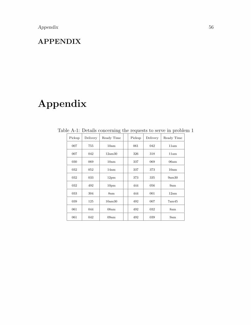
• Problem 1 can be found in Appendix in Table 1, where we have a set of 20

requests presented with 4 drivers available at 2 depots. These two depots are

described as follows:

- Depot 1: location number 498, time of departure: 7am. - Depot 2: location

number 498, time of departure: 12am.

• Problem 2 is presented in Table 2 and 3 of the Appendix. It concerns the

satisfaction of 85 requests, with 16 drivers available at 4 depots. These four

depots are described as follows:

- Depot 1: location number 498, time of departure: 7am. - Depot 2: location

number 498, time of departure: 8am. - Depot 3: location number 498, time of

departure: 11am. - Depot 4: location number 498, time of departure: 2pm.

The total number of locations in the network is 437 destinations. Each one corre-

sponds to a city, an address, and a point of access inside this location. The objective

is to obtain a complete schedule for each driver at each depot while maximizing

the total number of requests served by the fleet of vehicles and minimizing the total

mileage. A schedule consists of a description of the tour, with each step of the travel,

the time of arrival, the delay time and the time of departure at each location. A

schedule is organized as follow:


Tour :

The depot is depot N◦2

The driver is driver number : Dep2 Driv1

498 -. 064 -. 033 -. 515 -. 042 -. 444 -. 056 -. 444 -. 001 -. 498

Details :

Begin

Depot Location 498 at 6h0 - DELAY : 6h30

Empty -. 064 at 8h0 - Delay Time - 8h30

Request to -. 033 at 8h40 - Delay Time - 9h10








End


Parameters :

Length of 4 Requests in 356 miles.

Total Time : 765 minutes.

Time of driving : 465 minutes.

Delay Time : 300 minutes.

This study was more focused in observing the evolution of the time of computation

than in the generation of these schedules. Nevertheless, in the Appendix, we have

printed the schedule for the optimal solution for Problem 1, called Schedule 1.

4.2 Computational testing methodology

4.2.1 Description of the tests

We have coded our algorithms in C++ using the BCL library provided by Xpress-MP.

The tests consist of applying the heuristics presented in Chapter 3 to two problem

instances. We have applied the heuristics by changing the parameters described in

Chapter 3:

• r: we have choose to assign to this parameter the following values: 1, 2, 3,4,

5 and 50 requests served. First, we search and store all the tours that serve


at least one request. Of course, no path has a length of 50 requests served;

however, the case r = 50 means we do not compute any tours and we apply

the classical algorithm.

• m: Parameter m differs from problem 1 to 2. In the first case, we have applied

values 120, 240, 480 and 10,000 minutes. If m = 120 minutes, at each con-

struction of tours, we are able to add a request to this current paths only if the

ready time of this transportation request is between the current time t and (t -

120). The case m = 10,000 minutes means we do not restrict the choice of the

request. In the second problem that search to satisfy 85 requests, we were not

able to let this parameter become to bug, otherwise the computational time

explodes. We have done the tests for m = 30, 60, 90, 120 and 240 minutes.

This parameter makes us missed the optimality but we will see what is the

evolution of the solution. Trying to solve the problem with a parameter m

bigger than 240 minutes make the problem impossible to solve in a reasonable

CPU time.

• s: The total number of requests stored can take the values: 10, 100, 1000,

10000. If s = 10, we preload 10 tours per depot that will be used in the first

sub routine of the column generation.

First of all, we present the upper bound results from the Mosel model.


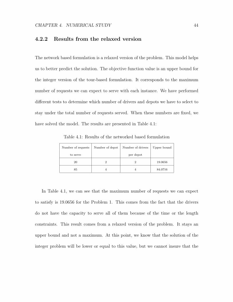
4.2.2 Results from the relaxed version

The network based formulation is a relaxed version of the problem. This model helps

us to better predict the solution. The objective function value is an upper bound for

the integer version of the tour-based formulation. It corresponds to the maximum

number of requests we can expect to serve with each instance. We have performed

different tests to determine which number of drivers and depots we have to select to

stay under the total number of requests served. When these numbers are fixed, we

have solved the model. The results are presented in Table 4.1:

Table 4.1: Results of the networked based formulation

Number of requests Number of depot Number of drivers Upper bound

to serve per depot

20 2 2 19.0656

85 4 4 84.0716

In Table 4.1, we can see that the maximum number of requests we can expect

to satisfy is 19.0656 for the Problem 1. This comes from the fact that the drivers

do not have the capacity to serve all of them because of the time or the length

constraints. This result comes from a relaxed version of the problem. It stays an

upper bound and not a maximum. At this point, we know that the solution of the

integer problem will be lower or equal to this value, but we cannot insure that the


tour-based formulation will reach this value. For Problem 2, Table 4.1 gives a value

of 84.0716 requests served with 16 drivers available at 4 depots.

4.3 Results

In Chapter 3, we have seen that we can combine these heuristics by crossing the

values of each parameter. Some cases have no meaning: for example, moving the

parameter s which decides how many paths we store in the case of r = 50. Sometimes,

two cases are the same.

For Problem 1, we have a set of 84 tests. Problem 2 concerns 105 different

instances solved. In Appendix, Tables 4, 5, 6, and 7, we present the following for

each test:

• The total number of tours stored for each depot

• The total number of requests served

• The optimistic total mileage

• The number of columns at the end of the resolution

• The CPU consumption in seconds


• The gap between the total number of requests served and the upper

bound value

The CPU consumption is a running time measured with the function XPRB::getTime()

inside the C++ code. The material used for these tests is a Pentium IV, 2.2 GHz,

256 Mo RAM. By observing these results, we will describe how the heuristics help

to decrease the computational time in the following section.

4.3.1 Interpretation

Problem 1

This part refers to Tables 4, 5, 6, and 7 of the Appendix. Case m = 10,000 minutes,

s = 1 requests and r = 10,000 tours fits to be the optimal case because the limits

are not restrictive. Here, we are storing all the tours preliminary. The column

generation only concerns pricing each tour inside this set of paths. The optimal

solution is 16 requests satisfied in 1672 miles. We will not find a better integer

solution. The minimum gap between the integer solution and the relaxed networked

based formulation is 3.0656. If we fix the value of the gap, it is impossible to find

an identical solution for this total mileage. But if we point out the total mileage for

each instance, we have the following results presented in Table 4.2.


Table 4.2: Evolution of the distance traveled versus CPU time

m s r Mileage Columns CPU (sec)

10,000 1 10,000 1,672 530 664

10,000 5 100 1,689 88 1,850

10,000 5 1,000 1,689 88 1,850

10,000 5 10,000 1,689 88 1,850

10,000 1 1,000 1,691 111 283

10,000 2 1,000 1,691 116 284

10,000 3 1,000 1,691 203 1,371

10,000 3 10,000 1,691 277 2,054

10,000 4 100 1,691 122 2,849

10,000 4 1,000 1,691 153 3,450

10,000 4 10,000 1,691 252 4,832

10,000 2 10,000 1,694 284 889

In Table 4.2, the results are ranked according to two criteria: the total mileage

first and the CPU consumption. (m; s; r) = (10,000; 1; 1,000) and (m; s; r) =

(10,000; 2; 1,000) propose a solution in less than twice the CPU time needed for the

optimal case. The time saved is essentially won by restricting the number of tours

stored preliminary. Although, this solution requires us to travel a total of 19 extra

miles. Storing all the feasible tours could be helpful to multiply the integer solution

serving 16 requests. Then, the choice of the shorter solution will be done between

more configurations. We can expect to achieve a better result regarding the total

mileage. This happens when we compute 10,000 tours per depots and the solution


proposed is 1,672 miles, compared to 1,691 miles in the case m = 1,000 tours. But

the consequence is the increase of the total time of computation.

When m is restricted to take a smaller value such 480 minutes, the whole search

of tours is affected by this restriction. Then, even if we decide to store all the feasible

tours as in the case (m; s; r) = (480; 1; 10,000), the optimal solution we can expect

to achieve is limited to be 15 requests served with a total mileage of 1,671 miles.

This comes from the fact that a lot of feasible tours have not been generated and

are not taken into account. Nevertheless, the total time to run this model is 102 sec

which is more than 6 times less than the one required to reach the optimal solution.

We can choose to lose some quality in the solution to save some computational time.

The classical Branch and Price algorithm represented with case (m; s; r) =

(10,000; 50; 10,000) has been stopped. In that case, we do not store any tours

in a first stage and at each generation we check each feasible path’s dual cost. This

solution is too long to be considered.

To conclude this example, it has been shown that adding a criteria restricting

the choice of the requests decreases the quality of the solution but saves a lot of

CPU time. By combining these parameters, we can expect to solve to optimality

this problem and generate a schedule in just a few minutes. We will see now how the


introduction of these parameters has influenced the resolution of a real size problem.

Problem 2

The situation is different in this second example because we are not able to reach the

optimality. Indeed, the size of the problem enables us to let our algorithm generate

some new tours randomly until optimality. This can not be done because checking

all the tours at each step of the column generation is a very time consuming task.

Chapter 3 studies the combinational aspect of the problem. Even trying to first

generate and then store all of them is totally impossible.

This is the reason why we are only able to compare each solution to the value

of the gap between the solution and the upper bound. Restricting the parameter

m to a small value like 30 minutes does not enable us to reach satisfactory results.

The upper bound of this solution space is 30 requests served. ∀ m, Case (s; r) =

(1; 10) and (s; r) = (1; 100) almost gives in a short amount of time a poor solution.

The conclusion is that generating a small number of tours of any size and preventing

them from generating new ones afterward does not provide a good solution.

In the Appendix, we first present the requests to serve in Tables 2 and 3. Then, the

results of each test are printed in Appendix in Tables 8, 9, 10, and 11. Some of these

tests have been stopped due to their length. The following Table 4.3 summarizes the


different configurations for which we achieve a solution of 54 requests served with

our set of drivers.

Table 4.3: Cases for which we achieve a solution of 54 requests served


240 4 1,000 7,012 257 3,961

240 2 10,000 7,012 652 4,407

240 4 10,000 7,012 226 4,422

240 3 1,000 7,012 242 4,755

240 3 10,000 7,012 174 5,353

First of all, the first remark we can make is that the solutions presented in this

array correspond to a case where the constraints on the choice of the requests are

less restrictive. Here, at each extension of a tour, we can select requests with a ready

time at 240 minutes maximum from the current time. The more flexibility you let in

the choice of the requests, the best solution you can expect to reach. But the CPU

time explodes according to this parameter.

The configuration that minimizes the most the CPU time is (m; s; r) = (240;

4;1000), where we generate in a first step 1,000 tours that serve at least 4 requests,

for each depot. This solution requires 3,961 seconds and generates 257 columns.

Some of these columns are tours that have been generated preliminary and some of

them come from the classical column generation. This second routine was restricted


to generate tours serving less than 4 requests.

A statement can be formulated: ∀ m, (s; r) = (4; 1,000) is almost the best case

every time. That comes from the fact that for this case we do not generate too many

tours, so we do not spend too much time to the preliminary routine. In a second

stage, during the generation process, we dispose of an interesting set of tours that

can enter the basis. So the second column generation routine is not called often.

And even when we call this routine, the generation of new tours is not restricted too

much by the parameter s: the tours can serve 1, 2, 3 and 4 requests, so we have a

chance to find some good feasible tours to enter the basis.

Case (s; r) = (2; 1,000) is also interesting because it takes less time for compu-

tation of the tours. We compute 1,000 tours that serve at least 2 requests. There

are less restrictions during the generation of them. Therefore, the total preliminary

generation takes less time. Even if the average length of the stored tours is shorter,

their computations are faster. Also, we save some time because the second column

generation routine can just generate some tours in length 1 or 2 requests.

The conclusion we can formulate concerning the choice of these parameters is

that we do not have to spend too much time in the first step. This means, do not

extend the parameter m too much because it enlarges our search. Also, we have to


limit the search of the tours to average length tours and not compute too many of

them (by restricting r to value like 1,000 paths). If such an option is selected, we can

expect to achieve a correct solution to this huge problem in a short amount of time.

If we analyze the situation for an optimum of 52 requests served, we notice an

important evolution in the CPU consumption. The results are presented in Table

4.4.

Table 4.4: Cases for which we achieve a solution of 54 requests served


120 4 1,000 6,433 198 2,879

120 4 10,000 6,433 174 3,214

120 3 1,000 6,433 187 3,456

120 3 10,000 6,433 145 3,890

120 5 100 6,433 120 4,208

120 5 1,000 6,433 120 4,208

120 5 10,000 6,433 120 4,208

240 4 100 6,433 304 4,695

120 5 10 6,433 243 5,342

240 3 100 6,433 265 6,278

Between the first and the last line, the CPU time is a multiple of two. Even if the

number of columns in case (m; s; r) = (120; 4; 1,000) is important, this generation is

fast due to the 1,000 tours per depot we dispose of. We can guess that an important


part of the columns comes from this set of tours. Generating a set of 10,000 tours per

depot requires some time at the beginning, but it helps to save some computational

time afterward because the classical column generation algorithm is called less often.

4.3.2 Conclusion

These tests were interesting to measure the effect of each parameter. Each of them

affects the solution differently by either the number of requests served or the total

mileage. Using these parameters inside a Branch and Price algorithm helps control

the resolution and the power of each routine. Solving a practical Pick Up and Delivery

Problem requires an important set of tours to assign to each available driver. If we

decide to use all the feasible tours, we will penalize the resolution by considering too

many paths. If we restrict the number of available tours too much, we can use the

resolution that will be quick but the solution provided will be very poor.

That is the reason why starting the resolution of such a problem with a set of

ready-to-use available tours can be an interesting strategy to achieve good results in

a short amount of time.

Chapter 5

Conclusion

Working on a transportation problem is a large task due to the complexity of the

problems and the multiplicity of the techniques that can be applied to them. In this

thesis, we have chosen to present some heuristics linked with the Branch and Price

algorithm. This technique is a combination of a branch and bound and a column

generation scheme. First of all, this classical algorithm needs to be understood and

coded. Two codes have been developed in parallel and then the branch and Price

algorithm has been finalized. The applications of this model on the first instance

have shown us which improvements to recognize.

Developing some heuristics for such a problem is very interesting because of the

immediate results we can get from them. Our heuristics concern some modifications

54

CHAPTER 5. CONCLUSION 55

in the classical way of processing with the Branch and Price algorithm. We have

demonstrated in Chapter 4 that the preliminary storage of tours and some restrictions

in the generation could be a way to decrease the computational time in a Branch

and Price algorithm. This approach to a solution does not have the expectation

to provide a complete solution for this real life problem. We were just concerned

in measuring the effect of the criteria on the computation of the schedules. These

contributions have the advantage to be easy to understand and efficient in saving

CPU time. The tests have been done on two different problems: one with 20 requests

to serve with 4 drivers and the other with a multi-depot problem that consists serving

85 requests with 16 drivers.

The multi-depot pickup and delivery problem with ready time presented in this

thesis does not take in account the partial truck loads. Furthermore, the truck are

assumed to be identical. Measuring the effect of our heuristics on a problem where

partial truck loads are added, could be interesting we stuck more to the reality. Also,

this kind of problem is guided by the demand. We can imagine introducing in future

work, a stochastic demand. Then the problem become much more complete and

realistic. With a random demand, the total expected cost of one day of service could

be computed. This information could be really useful for a company that search to

evaluate its logistics fees in advance.

Appendix 56

APPENDIX

Appendix

Table A-1: Details concerning the requests to serve in problem 1

Pickup Delivery Ready Time Pickup Delivery Ready Time

007 755 10am 061 042 11am

007 042 12am30 326 318 11am

030 069 10am 337 069 06am

032 052 14am 337 373 10am

032 033 12pm 373 335 9am30

032 492 10pm 444 056 9am

033 304 8am 444 001 12am

039 125 10am30 492 007 7am45

061 044 08am 492 032 8am

061 042 09am 492 039 9am

Appendix 57

Details concerning the Best solution for case 25 requests:

Schedule for each driver

The driver is driver number : Depot1 Driver1

Path Number 54: 498 -. 337 -. 069 -. 061 -. 044 -. 007 -. 755 -. 007 -. 042 -. 498

Depot Location 498 at 7h0 - DELAY : 7h30 -.

Request to -. 337 at 8h47 - Delay Time - 9h17 -.


Empty -. 061 at 12h2 - Delay Time - 12h32 -.






Empty -. 498 at 21h15 - Delay Time - 21h45 - END

Length: 4 Requests - Total Length: 885 min - Time of driving: 585 min - Total distance: 457 miles


Path Number 500: 498 -. 492 -. 007 -. 061 -. 042 -. 492 -. 039 -. 039 -. 125 -. 498












Appendix 58


Path Number 63: 498 -. 337 -. 373 -. 032 -. 052 -. 444 -. 056 -. 444 -. 001 -. 498













Path Number 173: 498 -. 030 -. 069 -. 033 -. 304 -. 492 -. 032 -. 032 -. 492 -. 498












Total mileage of the solution : 1672 miles - Total time of execution : 663.66 sec.

Appendix 59

Table A-2: Details concerning the requests to serve in problem 2 (1)


007 755 10 am 064 318 3 pm

007 042 12 am 30 064 033 7 am

007 044 2 pm 067 335 10 am

021 304 12 am 069 030 8 am

021 304 4 pm 125 039 5 pm

030 033 4 pm 318 304 12 am

030 069 10 am 318 304 6 pm 30

030 316 10 am 318 498 4 pm

032 052 2 pm 326 021 10 am

032 044 2 pm 326 021 11 am

032 492 10 pm 326 444 12 am

032 492 12 pm 326 318 11 am

032 493 10 am 337 373 10 am

032 042 2 pm 337 069 6 am

032 042 12 pm 337 069 12 am

032 033 12 pm 373 064 9 am 30

033 304 8 am 373 492 9 am 30

033 304 1 pm 373 335 9 am 30

033 304 9 am 30 444 056 9 am

033 304 9 am 15 444 056 10 am

033 304 4 pm 444 056 11 am

033 304 5 pm 444 304 6 pm

039 125 10 am 30 444 001 12 am

039 492 9 am 444 001 2 pm

044 515 1 pm 444 001 4 pm

044 061 10 am 444 001 6 pm

044 032 9 am 444 001 1 pm

044 032 11 pm 444 056 5 pm

Appendix 60

Table A-3: Details concerning the requests to serve in problem 2 (2)


044 061 11 pm 59 444 056 5 pm

050 069 9 am 444 001 6 pm

052 563 10 am 445 033 2 pm

052 044 12 am 445 316 3 pm

052 492 12 am 492 007 7 am 45

052 032 5 pm 492 032 8 am

061 044 8 am 492 033 8 am 30

061 052 8 pm 492 033 1 pm

061 042 9 am 492 039 9 am

061 042 11 am 515 042 4 pm

061 042 10 am 515 044 4 pm

064 335 12 am 563 032 8 am 18

064 373 3 pm 755 044 11 am

064 316 4 pm 974 056 9 am

515 039 10 am

Table A-4: Results of the tour-based formulation for Problem 1: 25 requests (1)

m s r N1 N2 Nserv Milage Columns CPU Gap

120 1 10 10 4 8 1,374 14 7 11.0656

120 1 100 26 4 8 1,374 12 7 11.0656

120 1 1,000 26 4 8 1,374 12 7 11.0656

120 1 10,000 26 4 8 1,374 12 7 11.0656

120 2 10 10 0 8 1,374 13 7 11.0656

120 2 100 22 0 8 1,374 12 7 11.0656

120 2 1,000 22 0 8 1,374 12 7 11.0656

120 2 10,000 22 0 8 1,374 12 7 11.0656

Appendix 61


m s r N1 N2 Nserv Mileage Columns CPU Gap

120 3 10 3 0 8 1,374 12 10 11.0656

120 3 100 3 0 8 1,374 12 10 11.0656

120 3 1,000 3 0 8 1,374 12 10 11.0656

120 3 10,000 3 0 8 1,374 12 10 11.0656

120 4 10 0 0 8 1,374 12 18 11.0656

120 4 100 0 0 8 1,374 12 18 11.0656

120 4 1,000 0 0 8 1,374 12 18 11.0656

120 4 10,000 0 0 8 1,374 12 18 11.0656

120 5 10 0 0 8 1,374 12 43 11.0656

120 5 100 0 0 8 1,374 12 43 11.0656

120 5 1,000 0 0 8 1,374 12 43 11.0656

120 5 10,000 0 0 8 1,374 12 43 11.0656

120 50 10 0 0 8 1,374 12 19 11.0656

240 1 10 10 10 8 1,073 20 5 11.0656

240 1 100 100 23 11 1,411 31 15 8.0656

240 1 1,000 114 23 11 1,523 32 22 8.0656

240 1 10,000 114 23 11 1,523 32 22 8.0656

240 2 10 10 10 9 1,211 22 7 10.0656

240 2 100 100 12 11 1,420 32 59 8.0656

240 2 1,000 110 12 11 1,523 32 60 8.0656

240 2 10,000 110 12 11 1,523 32 60 8.0656

240 3 10 10 10 11 1,411 30 60 8.0656

240 3 100 63 1 11 1,411 30 56 8.0656

240 3 1,000 63 1 11 1,411 30 56 8.0656

240 3 10,000 63 1 11 1,411 30 56 8.0656

240 4 10 4 0 11 1,420 32 642 8.0656

240 4 100 4 0 11 1,420 32 642 8.0656

240 4 1,000 4 0 11 1,420 32 642 8.0656

240 4 10,000 4 0 11 1,420 32 642 8.0656

Appendix 62



240 5 10 4 0 11 1,420 32 741 8.0656

240 5 100 4 0 11 1,420 32 741 8.0656

240 5 1,000 4 0 11 1,420 32 741 8.0656

240 5 10,000 4 0 11 1,420 32 741 8.0656

240 50 10 0 0 11 1,504 38 952 8.0656

480 1 10 10 10 9 1,181 25 5 10.0656

480 1 100 100 100 14 1,677 38 25 5.0656

480 1 1,000 481 303 15 1,671 52 102 4.0656

480 1 10,000 481 303 15 1,671 52 102 4.0656

480 2 10 10 10 11 1,651 35 20 8.0656

480 2 100 100 100 14 1,677 41 29 5.0656

480 2 1,000 477 286 15 1,671 50 103 4.0656

480 2 10,000 477 286 15 1,671 50 103 4.0656

480 3 10 10 10 13 1,623 49 457 6.0656

480 3 100 100 100 14 1,552 107 1,680 5.0656

480 3 1,000 422 139 15 1,671 51 126 4.0656

480 3 10,000 422 139 15 1,671 51 126 4.0656

480 4 10 10 10 15 1671 46 1,053 4.0656

480 4 100 100 12 15 1,671 57 945 4.0656

480 4 1,000 150 12 15 1,671 54 481 4.0656

480 4 10,000 150 12 15 1,671 54 481 4.0656

480 5 10 3 0 15 1,671 49 1,588 4.0656

480 5 100 3 0 15 1,671 49 1,588 4.0656

480 5 1,000 3 0 15 1,671 49 1,588 4.0656

480 5 10,000 3 0 15 1,671 49 1,588 4.0656

480 50 10 0 0 15 1,671 51 1,196 4.0656

Appendix 63



10,000 1 10 10 10 9 1,181 33 10 10.0656

10,000 1 100 100 100 11 1,329 29 65 8.0656

10,000 1 1,000 670 1,000 16 1,691 111 283 3.0656

10,000 1 10,000 670 3,127 16 1,672 530 664 3.0656

10,000 2 10 10 10 11 1,471 37 15 8.0656

10,000 2 100 100 100 13 1,481 41 43 6.0656

10,000 2 1,000 666 1,000 16 1,691 116 284 3.0656

10,000 2 10,000 666 3,110 16 1,694 284 889 3.0656

10,000 3 10 10 10 13 1,701 42 186 6.0656

10,000 3 100 100 100 15 1,652 49 257 4.0656

10,000 3 1,000 611 1,000 16 1,691 203 1,371 3.0656

10,000 3 10,000 611 2,877 16 1,691 277 2,054 3.0656

10,000 4 10 10 10 15 1,652 98 3,452 4.0656

10,000 4 100 100 100 16 1,691 122 2,849 3.0656

10,000 4 1,000 312 1,000 16 1,691 153 3,450 3.0656

10,000 4 10,000 312 1,641 16 1,691 252 4,832 3.0656

10,000 5 10 8 10 15 1,652 123 3,634 4.0656

10,000 5 100 8 83 16 1,689 88 1,850 3.0656

10,000 5 1,000 8 83 16 1,689 88 1,850 3.0656

10,000 5 10,000 8 83 16 1,689 88 1,850 3.0656

10,000 50 10,000 STOPPED

Appendix 64


m s r N1 N2 N3 N4 Nserv Mileage Columns CPU Gap

30 1 10 10 10 10 3 19 3,561 27 17 65.0716

30 1 100 26 100 28 3 30 5,072 42 86 54.0716

30 1 1,000 26 110 28 3 30 5,072 42 91 54.0716

30 1 10,000 26 110 28 3 30 5,072 42 91 54.0716

30 2 10 10 10 10 0 26 4,904 41 127 58.0716

30 2 100 23 100 23 0 30 5,072 42 97 54.0716

30 2 1,000 23 102 23 0 30 5,072 42 99 54.0716

30 2 10,000 23 102 23 0 30 5,072 42 99 54.0716

30 3 10 10 10 4 0 29 4,769 46 647 55.0716

30 3 100 14 76 4 0 30 4,948 47 571 54.0716

30 5 10 0 6 0 0 30 4,842 42 1,854 54.0716

30 3 1,000 14 76 4 0 30 4,948 47 571 54.0716

30 3 10,000 14 76 4 0 30 4,948 47 571 54.0716

30 4 10 2 10 0 0 30 4,870 42 1,450 54.0716

30 4 100 2 31 0 0 30 4,870 43 1,487 54.0716

30 4 1,000 2 31 0 0 30 4,870 43 1,487 54.0716

30 4 10,000 2 31 0 0 30 4,870 43 1,487 54.0716

30 5 100 0 6 0 0 30 4,842 42 1,854 54.0716

30 5 1,000 0 6 0 0 30 4,842 42 1,854 54.0716

30 5 10,000 0 6 0 0 30 4,842 42 1,854 54.0716

30 50 10 0 0 0 0 30 4,870 42 2,113 54.0716

60 1 10 10 10 10 10 23 4,041 39 22 61.0716

60 1 100 100 100 93 18 33 4,810 60 178 51.0716

60 1 1,000 240 640 93 18 43 5,933 362 1,348 41.0716

60 1 10,000 240 640 93 18 43 5,933 362 1,348 41.0716

60 2 10 10 10 10 10 35 5,659 71 406 49.0716

60 2 100 100 100 84 10 38 5,393 77 345 46.0716

60 2 1,000 235 629 84 10 42 5,722 188 1,445 42.0716

60 2 10,000 235 629 84 10 42 5,722 188 1,445 42.0716

Appendix 65



60 3 10 10 10 10 1 41 5,694 456 3,456 43.0716

60 3 100 100 100 47 1 42 5,722 362 2,524 42.0716

60 3 1,000 198 551 47 1 42 5,722 144 1,765 42.0716

60 3 10,000 198 551 47 1 42 5,722 144 1,765 42.0716

60 4 10 10 10 9 0 43 5,933 245 4,345 41.0716

60 4 100 97 100 9 0 43 5,933 168 3,455 41.0716

60 4 1,000 97 328 9 0 43 5,933 124 2,948 41.0716

60 4 10,000 97 328 9 0 43 5,933 124 2,948 41.0716

60 5 10 6 10 0 0 44 6,370 88 3,345 40.0716

60 5 100 6 11 0 0 44 6,370 78 3,275 40.0716

60 5 1,000 6 11 0 0 44 6,370 78 3,275 40.0716

60 5 10,000 6 11 0 0 44 6,370 78 3,275 40.0716

60 50 10 0 0 0 0 STOPPED

90 1 10 10 10 10 10 24 4,165 46 22 60.0716

90 1 100 100 100 100 34 34 4,912 102 212 50.0716

90 1 1,000 665 1,000 235 34 46 6,632 350 1456 38.0716

90 1 10,000 665 2,079 235 34 48 6,735 245 1657 36.0716

90 2 10 10 10 10 10 35 5,470 92 630 49.0716

90 2 100 100 100 100 26 41 5,601 143 1,648 43.0716

90 2 1,000 660 1,000 225 26 47 6,517 139 1,050 37.0716

90 2 10,000 660 2,065 225 26 47 6,517 298 1,288 37.0716

90 3 10 10 10 10 4 44 6,370 101 1,148 40.0716

90 3 100 100 100 100 4 45 6,522 179 2,054 39.0716

90 3 1,000 603 1,000 166 4 48 6,735 158 1,657 36.0716

90 3 10,000 603 1,940 166 4 48 6,735 132 1,864 36.0716

Appendix 66



90 4 10 10 10 10 0 45 6,522 450 3,230 39.0716

90 4 100 100 100 37 0 45 6,522 198 2,434 39.0716

90 4 1,000 390 1,000 37 0 48 6,735 143 1,987 36.0716

90 4 10,000 390 1,560 37 0 48 6,735 113 2,239 36.0716

90 5 10 10 10 4 0 48 6,735 155 4,210 36.0716

90 5 100 15 25 4 0 48 6,735 97 3,857 36.0716

90 5 1,000 15 25 4 0 48 6,735 97 3,857 36.0716

90 5 10,000 15 25 4 0 48 6,735 97 3,857 36.0716

90 50 10 0 0 0 0 STOPPED

120 1 10 10 10 10 10 23 4,046 56 23 61.0716

120 1 100 100 100 100 63 28 4,025 69 211 56.0716

120 1 1,000 1,000 1,000 982 63 49 6,321 420 1,767 35.0716

120 1 10,000 1,515 6,264 982 63 51 6,321 278 1,986 33.0716

120 2 10 10 10 10 10 36 5,286 112 1,123 48.0716

120 2 100 100 100 100 52 38 5,352 106 893 46.0716

120 2 1,000 1,000 1,000 962 52 45 5,643 196 2,805 39.0716

120 2 10,000 1509 6,248 962 52 51 6,321 495 3,203 33.0716

120 3 10 10 10 10 8 45 5,643 145 2,945 39.0716

120 3 100 100 100 100 8 46 6,632 204 4,563 38.0716

120 3 1,000 1,000 1,000 780 8 52 6,433 187 3456 32.0716

120 3 10,000 1,349 4,962 819 45 52 6,433 145 3890 32.0716

120 4 10 10 10 10 0 46 6,632 543 4,609 38.0716

120 4 100 100 100 100 0 46 6,632 234 3,412 38.0716

120 4 1,000 678 1,000 456 0 52 6,433 198 2,879 32.0716

120 4 10,000 678 1,345 456 0 52 6,433 174 3,214 32.0716

Appendix 67



120 5 10 10 10 10 0 52 6,433 243 5,342 32.0716

120 5 100 34 65 12 0 52 6,433 120 4,208 32.0716

120 5 1,000 34 65 12 0 52 6,433 120 4,208 32.0716

120 5 10,000 34 65 12 0 52 6,433 120 4,208 32.0716

120 50 10 0 0 0 0 STOPPED

240 1 10 10 10 10 10 25 73 31 59.0716

240 1 100 100 100 100 100 29 89 289 55.0716

240 1 1,000 1,000 1,000 1,000 1,000 51 545 2,431 33.0716

240 1 10,000 STOPPED

240 2 10 10 10 10 10 37 5,219 145 1,545 47.0716

240 2 100 100 100 100 100 39 5,520 137 2,604 45.0716

240 2 1,000 1,000 1,000 1,000 235 47 6,517 254 3,859 37.0716

240 2 10,000 3,579 10,000 2,411 210 54 7,012 652 4,407 30.0716

240 3 10 10 10 10 10 47 6,517 188 4,052 37.0716

240 3 100 100 100 100 100 52 6,433 265 6,278 32.0716

240 3 1,000 1,000 1,000 1,000 1,000 54 7,012 242 4,755 30.0716

240 3 10,000 2,543 10,000 1,989 198 54 7,012 174 5,353 30.0716

240 4 10 10 10 10 10 47 6,517 706 6,342 37.0716

240 4 100 100 100 100 100 52 6,433 304 4,695 32.0716

240 4 1,000 1,000 1,000 987 96 54 7,012 257 3,961 30.0716

240 4 10,000 1,267 8,453 987 96 54 7,012 226 4,422 30.0716

240 5 10 STOPPED

240 5 100 STOPPED

240 5 1,000 STOPPED

240 5 10,000 STOPPED

240 50 10 STOPPED

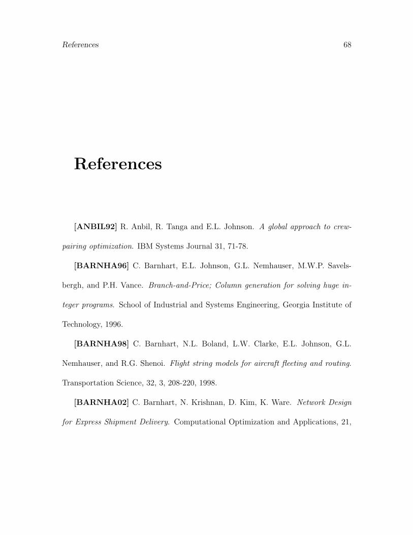
References 68

References

[ANBIL92] R. Anbil, R. Tanga and E.L. Johnson. A global approach to crew-

pairing optimization. IBM Systems Journal 31, 71-78.

[BARNHA96] C. Barnhart, E.L. Johnson, G.L. Nemhauser, M.W.P. Savels-

bergh, and P.H. Vance. Branch-and-Price; Column generation for solving huge in-

teger programs. School of Industrial and Systems Engineering, Georgia Institute of

Technology, 1996.

[BARNHA98] C. Barnhart, N.L. Boland, L.W. Clarke, E.L. Johnson, G.L.

Nemhauser, and R.G. Shenoi. Flight string models for aircraft fleeting and routing.

Transportation Science, 32, 3, 208-220, 1998.

[BARNHA02] C. Barnhart, N. Krishnan, D. Kim, K. Ware. Network Design

for Express Shipment Delivery. Computational Optimization and Applications, 21,

References 69

239-262, 2002.

[BODIN83] L. Bodin, B. Golden, A. Assad, and M. Ball. Routing and Schedul-

ing of vehicle and Crews: The State of the Art. Computers and Operations Research,

10, 62-212, 1983

[BORNDO01] R. Borndorfer, M. Grotschel, and A. Lobel. Duty Scheduling in

Public Transit. Konrad-Zuze-Zentrum Berlin. Takustr. 2001

[CHIANG97] W.C. Chiang adn R. Russel. A reactive Tabu Search metaheuris-

tic for the vehicle routing problem with Time Windows. INFORMS, Journal on

Computing, 9, 417-430, 1997.

[CHRIST98] M. Christiansen, B. Nygreen. A method for solving ship routing

problems with inventory constraints. Annals of Operations Research, 81, 357-378,

1998.

[CLARKE96] L.W. Clarke and P. Gong. Capacitated Network Design with

Column Generation. 1996.

[DANTZI54] G.B. Dantzig, R. Fulkerson and S.M. Johnson. Solution of a

large-scale traveling salesman problem. Operations Research 2, 393-410, 1954.

[DANTZI60] G.B. Dantzig and P.Wolfe. Decomposition principles for linear

programs. Operations Research, 8, 101-111, 1960.

[DESROC89] M. Desrochers and F. Soumis. A column generation approach to

References 70

the urban transit crew scheduling problem. Transportation Science, 23, 1-13, 1989.

[DESROS95] J. Desrosiers, Y. Dumas, M.M. Solomon, and F. Soumis. Time

Constrained Routing and Scheduling. In M.O. Ball, T.L. Magnanti, C.L. Monma,

and Nemhauser G.L., editors, Network Routing, Handbooks in Operations Research

and Management Science, 8, 35-139. 1995.

[DUMAS91] Y. Dumas, J. Desrosiers, and F. Soumis. The Pickup and Delivery

Problem With Time Windows. European Journal of Operational Research, 54, 7-22,

1991.

[FISHER95] M. Fisher. Vehicle routing. Handbooks in Operations Research

and Management Science, 8, 1-33, 1995.

[FORD58] L.R. Ford and D.R. Fulkerson. A suggested computation for maximal

multi commodity network flows. Management Science, 5, 97-101. 1958.

[GLOVER90] F. Glover. Tabu Search I. ORSA Journal on Computing, 1, 190-

206, 1989. Tabu Search II. ORSA Journal on Computing, 2, 4-32, 1990.

[HOFFMA93] K.L. Hoffman and M. Padberg. Solving airline crew scheduling

problems by branch-and-cut. Management Science, 39, 657-682, 1993.

[HJORRI97] Hjorring, Hansen. Column generation with a rule modeling lan-

guage for airline crew pairing. International Symposium on Mathematical Program-

ming Lausanne, 1997.

References 71

[LI02] H. Li , A. Lim. Local search with annealing-like restarts to solve the ve-

hicle routing problem with time windows. Proceedings of the 2002 ACM symposium

on Applied computing. 560-565. 2002.

[LEUNG90] J.M.Y. Leung, T.L. Magnanti and V. Singhal. Routing Point-

to-Point Delivery Systems: Formulation and Solution Heuristics. Transportation

Science, 24, 245-260, 1990.

[LANDRI01] A. Landrieu, Y. Mati and Z. Binder. A tabu search heuristic

for the single vehicle pickup and delivery problem with time windows. Journal of

Intelligent Manufacturing, 12, 497-508, 2001.

[LAPORTE92] G. Laporte. The vehicle routing problem: An overview of exact

and approximate algorithms. European Journal of Operational Research, 59, 345-358,

1992.

[LOBEL99] Lobel A. Solving Large-Scale Multiple-Depot Vehicle Scheduling

Problems. In N.H.M. Wilson, ed. Computer-Aided Transit Scheduling. Lecture

Notes in Economics and Mathematical Systems, Springer, 193-220, 1999.

[NEWHAU88] G.L. Newhauser and L.A. Wolsey. Integer and Combinatorial

Optimization. Wiley, New York. 1988.

[RIBEIR94] C.C. Ribeiro and F. Soumis. A column generation approach to the

multiple-depot vehicle scheduling problem. Operations Research, 42(2), 41-52, 1994.

References 72

[SAVELS95] M. W.P. Savelsbergh and M. Sol. The general Pickup and Delivery

Problem. Transportation Science. 29, 17-29, 1995.

[SAVELS97] M.W.P. Savelsbergh. A Branch-and-Price Algorithm for the gen-

eralized Assignment Problem. Operations Research, 6, 831-841, 1997.

[SEXTON85] T.R. Sexton and L.D. Bodin. Optimizing single vehicle many-to-

many operations with desired delivery times: I, Scheduling. II, Routing. Transporta-

tion Science, 19, 378-435, 1985

[SIGURD96] M. Sigurd, D. Pisinger and M. Sig. The pick up and delivery

problem with time windows and precedences. Dept Computer Science, University of

Coppenhagen, Denmark,

[SOL94] M. Sol and M. Savelsberg. A branch and price algorithm for the pick up

and delivery problem with time windows. COSOR Memorandum, 94-22, Eindhoven

University of technology, 1994

[SOLOMO87] M. M. Solomon. Algorithms for the Vehicle Routing and Schedul-

ing Problem with Time Window Constraints. Operations Research, 35, 254-265,

1987.

[VANCE96] P.H. Vance, C. Barnhart, E.L. Johnson, and G.L. Newhauser. Air-

line Crew Scheduling: A new formulation and decomposition algorithm. Operations

Research, 1997.

References 73

[VANDER96] F. Vanderbeck, L.A. Wolsey. An exact algorithm for IP column

generation. Operations Research Letters, 19, 151-160, 1996.

[VASEK83] V. Chvatal. Linear Programming. W.H. Freeman and Company,

1983.

[XUCHEN01] H. Xu, Z.L. Chen. Solving a practical pickup and delivery prob-

lem. Department of Systems Engineering, University of Pennsylvania. 2001.

XPRESS-BCL Reference Manual - Dashoptimization - 176 pages.

Modeling with XPRESS-MP - Dashoptimization - 14 pages.

oklahoma university optimizing … · optimizing transportation decisions in a manufacturing supply...

Documents