(ojo) - a stationary schrödinger-poisson system arising from modelling of electronic devices.pdf

Forum Math. 2 (1990), 489-510 ForumMathematicum

© de Gruyter 1990

A Stationary Schrödinger-Poisson System Arising fromthe Modelling of Electronic DevicesFrancis Nier(Communicated by Pierre-Arnaud Raviart)

Abstract. This paper is devoted to the study of a Schrödinger-Poisson System in a bounded one-dimensional domain. These equations describe the confmement of electrons in the quantumwell of a heterostructure electronic de vice. Existence and uniqueness of a solution are provedfor such a System. The paper ends with an introduction to numerical methods for solving thisSystem.

1980 Mathematics Subject Classification (1985 Revision): 35J05, 35J10, 35J55, 82A55.

Introduction

A heterojunction ([!]) is a perfect plane junction between two semi-conductorcrystals of different electronic structures. Because of this difference, a potential wellappears near the interface which confines the electrons. The model which we presentin this paper has been proposed (with various modifications) by several authors ([l 6],[15], [4]). We assume that the problem is translationally invariant parallel to theheterojunction interface. Thus, it reduces to a one-dimensional problem posed in abounded domain [0, L], where 0 and L are the boundaries of the device.

The equations describe in a self-consistent way the equilibrium between theconfining potential and the repulsive interaction of electrons. At the point in [0, L]the potential (here "potential" means "potential energy" for electrons), is split in twoterms: V0(x) + V(x). The first term V0 is a given function of and contains theelectronic characteristics of the materials, the positive background Charge andpossibly the applied voltage. The second term Fis determined by the electron densityn (x) via the Poisson equation t

(o.i) - T ( * ) = -«(*) in(o,L)

Brought to you by | Heinrich Heine Universität DüsseldorfAuthenticated | 134.99.128.41

Download Date | 11/8/13 6:11 AM

490 F. Nier

with boundary conditions

(0.2) F(0) = 0, F(L) = 0.

In (0.1), the constant q is the elementary electric Charge and ε the permittivity of thematerial.

The density n(x) depends on the repartition of the electrons in a discrete set ofquantized energy levels, (£,·)*= i ... »· These levels are the eigenvalues of the stationarySchr dinger equation

(0-3) - ̂ ̂ + (K0 + V)yt = είΨι


(0.4) V«(0) = 0, Vj(L) = 0.

The efFective mass of electrons in the crystal is m and denotes the Planck constant.The eigenfunction \pi is supposed to be normalized by

(0.5)

To each eigenvalue ef of equation (0.3), also called energy level, is associated anoccupation factor nt. This occupation factor is equal to the number of electrons in thestate i at thermodynamical equilibrium. Its expression is derived from statisticalphysics ([1], [5]) and is, for a given temperature Γ,

(0.6) „^^

where kB is the Boltzmann constant and SF the Fermi level. The model usually neglectsthe effect of the highest energy levels which are hardly occupied by electrons becauseof the exponential decay of the occupation factor with respect to the energy.Therefore, we introduce the number N of levels taken into account s a parameter ofthe model which is infinite when describing the whole spectrum. The total density ofelectrons at a point χ is the combination of the total density of each state nh weightedby the probability |ψί(·χ)Ι2 of presence at point χ of an electron in the state i. Thisleads to

(0.7) «(*)= Σ «,Ιν,ΜΙ2·i= l

The Fermi level eF, which is an unknown in this problem, is determined by theequation which ensures the neutrality of the total electric Charge. In heterojunctionsthe positive Charge is localized in a zone with length L+, which is called in semi-conductor physics the doped zone, and its density n+ is a specific value of the device.Then the total positive Charge is L+. n+ and the electric neutrality reads

Lf n(x)dx = L+n+.



A Stationary Schrödinger-Poisson System 491

Because of the normalization of the eigenfunctions this can be written with (0.7)

(0.8) «i = £ + « + ·i=l

For the simplicity of the mathematical analysis, the description of the backgroundpositive Charge is contained in the potential V0 äs a data of the problem and oneremarks the additional equality

The quantities involved in this problem are lengths, energies and densities.Therefore we introduce the following scaling units: the length of the device L, thethermal energy kBT and the density n+. With these units we get the followingdimensionless variables and functions

- lengths:X — LJ X ? Lt _j_ — LJ M—i _j_

- energies:V(x) = (kBTYl V(xY V0(x) = (kBTYl V0(x)£f = (kB TY 1 ef , = (kB T)' 1 SF

- normalized eigenfunctions:

- densities:n(x) = (n+Yln(x), n{ = (Ln+Y1^.

With this scaling the Schrödinger equation comes out in the form

l(0.10) tpf(0) = 0, v5f(l) = 0,

where the length Ith is the scaled thermal wavelength, given by

1F

The Poisson equation becomes

(0.11) - J g l

(0.12)



492 F. Nier

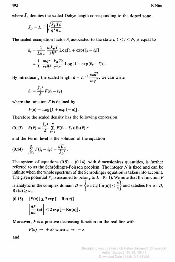
where ID denotes the scaled Debye length corresponding to the doped zone

Γ — r - 1A - L·!

l mkBT

The scaled occupation factor nt associated to the state /, l < ι < N, is equal toT

Log [l + exp(£F — ε^]

Log [l +exp(£F-8i)].

Ln+

l mg2 kBTs

By introducing the scaled length = L 1 T, we can writemq2

Γ 2/Z^-l-Ft -e,)

where the function F is defined by

F(w) = Log[l+exp(-w)].

Therefore the scaled density has the following expression

(0.13) n(X) = ̂ - Σ F(gt-ΒΡ)\{ρι(Χ)\2a t=i

and the Fermi level is the solution of the equationN ft T

(0.14) Σ Ρ(εί - 8F) = +

The System of equations (0.9)... (0.14), with dimensionless quantities, is furtherreferred to s the Schr dinger-Poisson problem. The integer N is fixed and can beinfinite when the whole spectrum of the Schr dinger equation is taken into account.The given potential F0 is assumed to belong to L °° (0,1). We note that the function F

in D = < ιu e C/\ Im(w) l < — > and satisfies for u e D,4J

is analytic in the complex domainRe(w) > MO,

(0.15) |F(M)|<2exp[-Re(M)]

dF ' * <2exp[-Re(w)].

Moreover, .F is a positive decreasing function on the real line with

F(w) -+ + oo when u ~> — oo

and




F(ü) -» 0 when u -> + oo .

These properties of the function F are the only ones that we need in our analysis.Especially, they ensure the existence and uniqueness of the Fermi level SF äs a solutionof equation (0.14): The first member of this equation is obviously a continuousdecreasing function which takes all positive real values when varies.

For simplicity, we will drop the notation ~ used for the scaled quantities whichappear in the Schrödinger-Poisson System. Since we usually consider real-valuedfunctions, the Sobolev spaces Lp(0,l; IR) and Wm'p(0,l; IR) are actually denoted byLp(0,l) and FF1"·* (0,1). We only precise L* (0,1; C) and fFm'p(0,l; C) in the complexcase.

Our main concern in this paper is the mathematical analysis of the Schrödinger-Poisson System. In Section l, we use the Schauder fixed point theorem to proveexistence of Solutions for this problem. Section 2 is concerned with a non-localmonotony property of the electron density with respect to the potential V.Consequences of this property are first the uniqueness of the solution, and secondlythe convexity of a functional, derived from thermodynamical considerations, whichtakes its minimum value at the solution of the Schrödinger-Poisson System. The lastpart (Section 3) is devoted to the numerical approximation of the solution. First, weprove the convergence of the solution of the model with finite N, towards the solutionof the model with N = oo, äs N -> oo. We end with a brief presentation of algorithmsused in numerical computations.

§ l Existence for the Schrödinger-Poisson System

In this Section, the number Nof eigenvalues of the Schrödinger equation involvedin the System (0.9) . . . (0.14) is fixed. To each potential Fin L °° (0,1) is associated theelectron density n(V) derived from eigenstates of the Schrödinger equation viarelations (0.13) and (0.14). A potential denoted by S(V) corresponds to this Chargedensity by solving the Poisson equation (0.11). Next we prove existence of Solutionsof the whole Schrödinger-Poisson System by applying the Schauder fixed pointtheorem to the mapping 5 äs it is done in [7].

Before developing these arguments and äs a first step in this analysis, it is natural tolook at the stationary Schrödinger equation for a given potential V in L00 (0,1).

1.1 The stationary Schrödinger equation

This part recalls some classical results while going into details and introducingnotations. Here we are interested in the eigenvalue problem for the operator H (V)definedinL2(0,l)by

whereBrought to you by | Heinrich Heine Universität Düsseldorf

Authenticated | 134.99.128.41Download Date | 11/8/13 6:11 AM

494 F. Nier

H =-λ2 —

The potentials F0 and V are supposed to be real functions which belong to L °° (0,1)and the domains of these operators are the same:

D(H(V)) = D(H0) = H2 (0,1) n H£ (0,1).

For this operator H (V), the theory of self-adjoint Sturm-Liouville operators([8], [13]) applies. The space L2(0,1) admits an orthonormal basis (t/\-)i=i...oo ofreal-valued eigenfunctions of the operator H (V) and each eigenvalue is real andsimple. In the sequel, the real number ef(F) is the /-th eigenvalue of the operatorH (V) and φ{ (F) denotes the corresponding normalized eigenfunction defined up to asign. At the moment, we don't have to precise the sign of \pt(F) since it appears onlyvia its modulus in the equations.

The regularity of the eigenvalues ef (F) with respect to the potential is a well knownproblem of inverse spectral theory ([13]) when the potential Fis taken in the spaceL2(0,1). In this framework, the mapping e f ( · ) : L2(0,1) -» IRis proved to be a realanalytic function of the potential whose gradient is given by

(1.1) f|(F) = |'

As a consequence, this gradient |ip f(-)|2 : L2(0,l) -> L2(0,1) is also a real analyticfunction of the potential V. Moreover, concerning the analytic continuation in acomplex domain, we know ([13]) that, for every real valued potential VE L2(0,1),there exists a neighborhood t/of K in L2 (0,1; C), where all the eigenvalues st extendanalytically. This neighborhood U is defined uniformly with respect to theeigenvalues εί5 and the gradients are still given by (1.1).

The continuity of the imbeddings L00(0,1) -> L2(0,1) and L2(0,1) -» L1 (0,1)yields the following result

Proposition 1.1 For any fixed integer i, the mapping

β|(·): KeL°°(0,l) ->and its derivative

are two real analytic functions. Moreover, for any given real potential V, there exists aneighborhood U (V} cz L °° (0,1; C), where the eigenvalues β,· are analytic functions withderivatives still given by (1.1).

Indeed, this proposition just replaces the scalar product and the hilbertian structureof the space L2 (0,1) by the duality between L00 (0,1) and L1 (0,1).




Because of the normalization of the wave function ? we have

L1

Let F be a real potential which belongs to L00(0,1). If V is taken in the complexneighborhood U( F), defined äs in Proposition 1.1, then the previous equality leads tothe estimate

which is uniform with respect to i. We notice that this result holds for any pair ofPotentials, F and F', when they are taken in the real space L00(0,1). In this case,estimate (l .2) is also given by a much simpler analysis based on the min-max principlefor self-adjoint operators ([3]). By taking V = — F0, this implies the followingasymptotic behaviour of the eigenvalues sequence e^F), = l ... oo,

which is also given in [13].Next we precise the derivative of the mapping

FeL°°(0,l) -> Iv^F^eL^O,!)which we will need further when differentiating the electron density with respect tothe potential. For this, let FeL°°(0,l) be a fixed potential and FeL°°(0,l) adirection for Computing the directional derivative. For any complex number ß,h(ß)denotes the operator:

h(ß) = H(V + ßA V) = ~ + (Vo + K) + ß* V.

Lemma 1.1 Let i denote a fixed integer. There exist a positive number R > 0 and aunique pair ( , ) of analytic functions

s:ße{zeC/\z\<R} -* e ( ß ) e Cand

ip:ße{zeC/\z\<R} -+ v(ß)eL2(09l;C)such that ( ) is a simple eigenvalue ofthe operator h(ß) and\p(ß) the correspondingnormalized eigenfunction, which both satisfy

with

(1.4)Brought to you by | Heinrich Heine Universität Düsseldorf


496 F. Nier

Moreover, we have

Proof. This local regularity result for eigenfunctions is a consequence of theperturbation theory of linear operators ([14], [10]). The family (A(/0)> ßeC,satisfies the properties:

(i) For each complex /?, h(ß) is a closed operator with the domain D(HQ)independent of ß.

(ii) For each vector e D(/f0), h(ß) - is an analytic function of ß.

(iii) If ß is real then the operator h(ß) is self-adjoint.

With these three conditions and because ef ( F) is a simple eigenvalue isolated from therest of the spectrum of H(V) = A(0), the Kato-Rellich theorem ([14], [10]) appliesand states the existence and uniqueness of the locally defined pair ( , ) of analyticfunctions of ß (\ ß\ < R). Thanks to the uniquenes, one can identify, for ß e IR and\ß\ < R, ( ) with e f(F+ ßA V) and \p(ß) with £( + V\ while noticing thatcondition (1.4) specifies (at least locally) the sign of the eigenfunction \pi(V+ ßA V}.Then equality (1.1) yields

For simplicity, we introduce the following notations

° = (0), °

For 0, the function tp(/J) e L2 (0,1) is an eigenfunction of h(ß) and this impliesthe equality

By taking the limit of these expressions when ß -* 0 we get, since A(0) is a closedoperator,

1 e/>(A(0)) = H2 (0,1)0^(0, 1)and

(1.6)Brought to you by | Heinrich Heine Universität Düsseldorf


A Stationary Schr dinger-Poisson System 497

The derivative — (0) = ψ 1 is obtained via its components on the orthonormal basisdin L2 (0,1) of eigenfunctions of the operator A(0) = H (V) : (ipj(VJ),j = l . . . oo. Forthis we take the scalar product of equality (1.6) with each vector v^(F), j Φ ι,

(x)dx = 0

The component oft/; 1 with respect to the direction t/;f(F) is proved to be equal to zeroby differentiating the normalization condition

As a remark, taking the scalar product of (1.6) with the vector φ° gives again thedsexpression of the derivative — (0). Gd

Since the two functions β -> ipi(V+ AV) and β -> ψ ( β ) can be identified locallyfor β on the real axis, we have immediately the derivative with respect to V of theanalytic function |tM')l2 : £°°(0,1) -> L1^,!).

Proposition 1.2 Lei Vbelong toL°°(0,l). The derivative -~- (V) at thepoint Visa

mapping: Δ FeL°°(0,l) o V

(1.7)

j= l

From the physical point of view, the expressions (1.1) and (1.5) are in fact the basicformulas of the first order perturbation theory developed in quantum mechanics.Here we have just specified the spaces in which the mappings are defined so that wecan use further the classical tools of functional analysis.

1.2 Existence for the Schr dinger-Poisson System

Now, we consider the whole coupled Schr dinger-Poisson System (0.9) . . . (0.14)and we establish in this section the following result

Theorem 1.1 There exists a solution in L00^,!) of the Schr dinger-Poisson system.



498 F. Nier

In the previous section, we have defined the functions V -+ ef(F), i = l ... oo. Then,by taking Neigenvalues, we know that equation (0.14) determines uniquely the Fermilevel referred to äs 6F(F), thanks to the properties of the function F. Thus we candefine the density äs a function of the potential

«:FeL°°(0,l) -> n(V)eLl(Q9l)

by

(1.8) n(V)(x) = & J; F(si(V)-sF(V))\ipi(V)(x)\2.

Definition 1.1 We define the map S: L °° (0,1) -> L °° (0,1) so that S(F) is the solutionof the Poisson equation

(\ Q^ _ ;2\JL .yJ — Ajp _ 2

(1.10) S(F)(0) = i

Indeed, a solution of the System (0.9)... (0.14) is a fixed point of the mapping S. Wedemonstrate the existence of such a solution by proving that the Schauder fixed pointtheorem ([9]) applies. Equations (0.13) and (0.14) yield the equalities

12|U25(F)" H dx2

Therefore we introduce the set K defined äs the closure in L00(0,1) of the convexsubset

d 2

dx2 V F(0)=D

Thanks to the boundary conditions (1.10), the Poincare inequality gives the uniformboundedness of the norm ||5(K) 11^2,1. Thus, the compactness of the imbeddingFF2'1 (0,1) c L00(0,1) leads to the following result

Proposition 1.3 The set K is a compact convex subset in L °° (0,1) such that S(K) c: K.

The last ingredient in order to use the Schauder fixed point theorem is thecontinuity of the mapping 5 which is an immediate consequence of the continuity ofthe density with respect to the potential. Because we already know that 8f(F) and|t/>i(F)|2 are analytic functions of the potential, this continuity relies only on theregularity of the Fermi level 6F(F). Indeed we have much more regularity for theFermi level:

Proposition 1.4 The mapping BF : L00(0,1) -> R is a real analytic function of thepotential and its derivative is given by




; denotes the negative real number

(1.12) a,(K) =

Proof. Let J7(F) c L °° (0,1; C) be a bounded complex neighborhood of Fin which allthe eigenvalues ε, are analytic and satisfy

VK'et f (F) ,

where the constant C depends only on F and on the diameter of U (V}. Such aneighborhood can be found thanks to the estimates (1.3) and (1.4) and because thedomain of analytic extension of the eigenvalues ef can be chosen uniformly withrespect to the integer i (Proposition 1.1).

Next, let W denote the complex domain

W=\zeC/\z-sF(V)\< ~l o

We consider the function C~ defined in W κ U (V) by

5}·The analyticity of F in the domain D = < u e C/\ Im (M) | < — > ensures that each term

of the sum which defines C~ is an analytic function with respect to(z, Vf)eW* U (V). Moreover, the exponential decay of F( ) when Re(w) -> + oogiven by (0.15) associated with (1.14) yields the normal convergence of the series forN = oo. In this case, C ~ is the uniform limit of a sequence of analytic functions andtherefore is analytic in W χ U (V} ([13], [12]) s well s for a finite N. At the point(eF, F), we have

C - (eF9 F) = Σ F(*t(V) ~ *F) = r

and

8C~ N 8F

dFbecause the eigenvalues ;(F) are real and -r— is negative on the real line.οε



500 F. Nier

Then, the implicit function theorem ([13], [12]) applies and yields the analyticityof the mapping V -* £F(V) in the domain of real potentials. Using the notation(1.12), the derivative of SF with respect to V is then given by

Σ«,·(ην'=1

From this result concerning the Fermi level eF, we get the analyticity with respect tothe potential of each term of the sum which defines the density in (l .8). Therefore themapping n : L °° (0,1) -> L1 (0,1), defined for a finite number N of eigenvalues, is realanalytic. In the case N = oo, the same argument of normal convergence s in theprevious demonstration applies this time for L1-valued series, thanks to thenormalization of the eigenfunctions. Thus the mapping n is also analytic in this case.Since the mapping S is the composition of n with a bounded linear operator, given bysolving the Poisson equation (1.9), S is also a real analytic function of the potential.

Proposition 1.5 Themappings n : L00 (0,1) -> L1 (0,1) and S: L°°(0,l) -> L«>(Q,l)arereal analytic functions.

The mapping S: L00(0,1) -> L00(0,1) is continuous and sends L00(0,1) to thecompact convex subset K. Then the Schauder fixed point theorem applies and thisends the proof of Theorem 1.1.

Remark 1.1 This analysis actually needs much less regularity than we have for themapping S: we only used continuity. Therefore, it can be extended to more involvedmodels which describe heterojunctions. As an example, Theorem 1.1 is still valid ifthe ion density is a nonlinear continuous function of the potential. Such a model isproposed in [15] and takes into account the effects of the potential on the ionizationof atoms.

§ 2 Monotony for the density n (V) and applications:Uniqueness and equivalence with a minimization problem

2.1 Monotony and uniqueness

The previous analysis proves the analyticity of the density n (V) with respect to thepotential Ftaken in L °° (0,1). Moreover, using relations (1.1), (l .7) and (1.11), we areable to compute the derivative of the density with respect to the potential. This leadsto a monotony property of the density which yields uniqueness for the Schr dinger-Poisson system.




Proposition 2.1 Lei V and A V be in L °° (0,1); we have

(2.1) f [n(V+ A V)- w(K)](jc) Δ V(x)dx < 0.

Proof. By Proposition 1.5 we know that the density is a real-analytic function of thePotential. Let us prove that

from which (2.1) follows at once. The derivative of the density is the sum of two terms

where

anddn1ΓΓ, = Σ F(e,-eF δ V

Let Fe L10 (0,1) denote a fixed potential and Δ Fe L00 (0,1) be the direction alongΛ p ^ P.

which we differentiate. Replacing -— ̂ and —7 by their expressions (1.11) and (1.1)o V oV

gives for the first term

U* ι

where the real number af is defined by (1.12). This is an antisymmetric expressionwhich can be written

Since the real numbers af are negative, we have the estimate



502 F. Nier

![(£), H WJKW

= ( Σ «,·) * Σ *i*j Γί (IIP,\j=l / l<i<j<N |_0

< 0.

For the second term of the derivative of the density, the relation (1.7) yields

N C oo 2 Γ1 1= Σ J*(fi, - eF) < Σ f ^ Vipwjdx \ViVj

i= i U=i i - f i jLo J

+ 2 Σ ε,· — EJ

Thus we have

— l -AV\(x)AV(x)dx

= 2 Σ :

+ 2l ?swN<j<oo

Since F is a positive decreasing function, this yields the estimate

which ends the proof. D

Remark 2.1 The density n(V) is the electron density at equilibrium in the givenPotential V. If the increment of potential A V(x) is a "localized" positive function("localized" means that the support of Δ Fis small compared to the interval [0,1]),the electron density has to decrease globally in the support of Δ Fso that the estimate(2.1) is satisfied. Then, this monotony property appears s a mathematical translationof the tendency of electrons to occupy low potential areas at equilibrium. We noticethat this result strongly relies on the decay of occupation numbers with respect to theenergy, which physically ensures the stability of equilibrium. Such a monotonyproperty holds for the System coupling stationary drift-diffusion with Poissonequations ([l 1]). Despite the fact that this latter model, also used for semi-conductor




devices, does not take into account quantum mechanics, this inequality retains thesame physical meaning.

We are now able to state

Theorem 2.1 The Schrödinger-Poisson System has a unique solution V which belongs toL «(0,1).

Proof. Let us assume that Vl and F2 are two Solutions of the Schrödinger-PoissonSystem. They are both in the compact subset K defined in Section l and satisfy thePoisson equation


F(0) = F(l) = 0.

Estimate (2.1) applies with V = Vi and V = V2 - Vl

J \n(V2)(x) - n(y1)(x)'](V2(X) - V,(x))dx < 0

and gives

After integrating by parts, we obtain the following inequality

WA sowhich implies V2 = FI . D

- »a]1

2.2 The Schrödinger-Poisson System äs a minimization problem

In this part, we show that the solution of the whole Schrödinger-Poisson System isthe potential which minimizes an energy functional. Indeed, the physical problemmodelled by the Schrödinger-Poisson System describes the thermodynamical andelectrostatic equilibrium of electrons in a confining potential. Therefore the naturalenergy associated with the population of electrons is their free energy. Such athermodynamical quantity is derived from the Fermi-Dirac statistics associated withthe initial three-dimensionnal problem, in a similar course of reasoning äs that usedfor the occupation numbers ([1], [5]). Let us introduce the scaled free energy

: Fe //o1 (0,1) -» (V) 6 R defined by:2 N +°° l

= -? Ffe - SF)SF - J F(u)du .i-1L *-eF J



504 F. Nier

Because of the continuity of the imbedding HQ (0,1) <= L °° (0,1), this mapping φ isalso a real-analytic function of the potential V in HQ (0,1). With the previous results,we can compute its derivative which belongs to H'1 (0,1),

By differentiating (0.14), we obtain

so that the first term vanishes. Moreover, the equality (1.1) which gives the derivatives3ε·-1, still applies and leads to the result

(2,2) (F) =

Now the estimate (2.1) appears s a convexity inequality which states the convexity ofthe functional — φ.

As we have seen in Section 1.1, the Schr dinger-Poisson System can be written:

lF(0)=F(l) = 0 '

As a consequence of relation (2.2), this equation is the Euler equation associated withthe unconstrained minimization problem ([2], [6])

;2 ι Λ/ιΛ2(2.3) Inf /(F); /(K) = -^Mf_J άχ-

This function / is real-analytic and convex s the sum of two convex functionals.Moreover since the first term is a coercive quadratic form in //o (0,1), the secondderivative of / is uniformly coercive which entails existence and uniqueness of thesolution of (2.3).

Theorem 2.2 The minimization problem (2.3) is equivalent to the Schr dinger-PoissonSystem and has a unique solution in HQ (0,1).

Remark 2.2 Similar results can be easily obtained for another physical problem wherewe assume only the electrostatic equilibrium of electrons without assuming thethermodynamical equilibrium. This problem is modelled by a simpler Schr dinger-Poisson System: In this case, the occupation factors are given numbers nh i = l ... N,




independent of the potential V and there is no equation similar to (0.14) fordetermining the Fermi level. If the sequence (wf) is decreasing, then the whole analysisconcerning existence, uniqueness and monotony of the density still holds. Moreover,this problem can be also viewed s a minimization problem (2.3) where the function φis replaced by the function φ0 defined by

Ψο(*0= Σi= l

and we have again

(2.2)

In this case where the free energy becomes meaningless, this quantity 00 is thecharacteristie energy and describes the total energy of electrons.

§ 3 Numerical resotution of the Schr dinger-Poisson System

Numerical computations cannot handle an infinite set of eigenvalues andeigenfunctions. For numerical purpose, one uses a finite (and rather small) number ofenergy levels. This is generally admitted to approximate the physically relevant modelwhich incorporates all the energy levels. In the sequel, we prove that the truncation ofthe spectrum results in an error of the order e ~CN2 when the number N of energy levelstends to infinity. Then we propose algorithms for solving numerically the model usinga finite number N of eigenstates.

3.1 Asymptotic behaviour of the solution when 7V goes to infinity

In this part VN denotes the unique solution of the System (0.9) ... (0.14) for a fixednumber N of eigenstates, possibly infinite. In the same way, the mappings sj and nN

are the one defined in the previous section but for a fixed N.

Theorem 3.1 There exists a positive constant C so that thefollowing estimate holds forlarge N

(3-1) \\K-VN\\L^Ce-^"2N2.

Proof. The map nN: V -> wN(F)satisfiesthemonotonyproperty(3.1).Thenwehave:

j [nN(V„)(x) - MK)(*)][F„(x) - Ktf dx <ί Ο

and consequently



506 F. Nier

Since the difference VN — ϊ£ satisfies homogeneous Dirichlet boundary conditions,we have the estimate

i v — V II\ r N * ο οΙΙί , °L2

By combining the above inequalities, we obtain

This leads to

(3.2) || VN - % ||LOo < - ΓLi Σ - sf) - Ffr - s») |

where we have omitted the argument V^ in the expressions sh s^ and sj.Next we set

= Σ

Using the asymptotic behaviour of st given by (l .3), there exists a constant C such that

μΝ < Ce~*2**2N2 for large N.

Let us prove

(3.3) £ lFfe - ei?) - Ffa - e£) i = ̂ -

By definition, the two real numbers ej? and ε" are the Solutions of the followingequations

N njτι r*/_ _oo\ "^ +

andBrought to you by | Heinrich Heine Universität Düsseldorf



V J7/ N\ _ ^ +

Since Fis a positive decreasing function, this implies that sj? is smaller than s* so that,for every ι in {l ... N},

This yields identity (3.3). By combining (3.2) and (3.3), we obtain the desired bound(3.1). D

3.2 A relaxation method

Let us study a classical relaxation method that physicists have already used innumerical computations ([15]). This algorithm is written

(3.4) F" + 1 = (l - ω) Vn + coS(Vn)

with the initial data F° e K. The parameter ω belongs to the interval [0,1] and has tobe chosen properly in order to ensure the convergence of the method, s stated in thefollowing result:

Theorem 3.2 Let V denote the solution of the Schr dinger-Poisson system (0.9) ...... (0.14). There exists a real number ω0 6 ]0,1] so that for every ω, Ο < ω < ω0, thesequence (F") defined by (3.4) converges to V with:

dtic(

L2

and

Proof. With the notation Fn+1/2 = S(F"), we have

(3.5) Fn+1 - V = (l - ω) (K" - F) + ω(Κ"+1/2 - F)

and

(3.6) - ( F » + 1 - F )

By multiplying (3.5) by (3.6) and integrating over χ e [0, 1], we obtain



508 F. Nier

>"'-_ J7)M L 2

— (y»- K) 2 + ω2

L2

" (lsn+1/2dx(y F)

+ 2ω (l - ω) f Γ - ̂ -2 (F"+1 /2 - F)l

The Poisson equation gives

[Fn- F]i/;c.

Combining the monotony property (2.1) with the previous equality gives

Therefore, we have

s^'-^L._«,)= JL(r-

L2

Moreover, an Integration by parts yields

_:iLrFw+1/2_(Fw+1/2-F)L2

Since Vn+ 1/2 and F belong to the bounded subset KofL00 (0,1), and thanks to theanalyticity of the mapping n, there exists a constant C such that

II αχ ||L2

Then, by the Poincare inequality, we have

i/JC/«+1/2 _ <c

L2

As a consequence, we get finally

dx L2where

^-(F"-F)

ρ(ω) = l/l-Brought to you by | Heinrich Heine Universität Düsseldorf



Note that ρ (ω) satisfies ρ (ω) < l when ω e ( 0,

The optimal convergence rate depends on the physical parameters Ath, λβ and awhich appear in the dimensionless Schr dinger-Poisson System. Numerical compu-tations show that the convergence rate is very sensitive to the variations of theParameter λΌ. Especially, for small values of λβ, this relaxation method happens to beunefficient because of an optimal convergence rate very close to l . This has motivatedthe investigation of other algorithms.

3.3 Other algorithms

The formulation of the Schr dinger-Poisson system s a minimization problem(Section 2.2) provides a wide variety of algorithms which have already beendeveloped in optimization theory ([2], [6]). As a remark, the relaxation methodstudied in the previous part can be considered s a fixed step gradient method.Actually, the gradient of the function / defined in the space ^(Ο,Ι), provided with

the usual scalar product (u, v) = \-r~T~^x^ *s easity seen to be given by0 w X ClX

F/(F)= F-S(F)

so that the Iteration scheme (3.4) can indeed be written in the form

Actually, in order to minimize a convex functional there are much more efficientalgorithms than this one such s, for example, the conjuguate gradient method orNewton method. The uniform coerciveness of the second derivative of the function /ensures the theoretical convergence of these algorithms. But first attempts in usingthese algorithms also failed for small values of the parameter AD. Indeed, for small ΑΡ,the minimization of the functional /is an ill-conditioned problem for which we needmore involved algorithms such s a preconditioned conjuguate gradient method orcontinuation algorithm applied to the Newton method. A detailed study of thesealgorithms and numerical comparisons between them will be reported in aforthcoming paper.

References[1] Ando, Fowler, Stern: Electronic properties of 2D Systems. Rev. Mod. Phys. 54 (1982), 437[2] Cea, J.: Optimisation: Theorie et algorithmes. Dunod, Paris 1971[3] Courant, R., Hubert, D.: Methods of Mathematical Physics. Wiley 1962[4] Degond, P, Guyot-Delaurens, F., Mustieles, F.J., Nier, F.: Particle Simulation of a

bidimensional electron transport parallel to a heterojunction interface. Compel (toappear)

[5] Feynman, R.P.: Statistical mechanics: a set of lectures. Frontiers in Physics. W. A.Benjamin, London 1972



510 F. Nier

[6] Gill, P.E., Murray, P.E., Wright, M.H.: Practical Optimization. Academic Press, NewYork 1981

[7] Greengard,C., Raviart,P.A.: A boundary value problem for the stationary Vlasov-Poisson equations: the plane diode. Comm. Pure and Appl. Math, (to appear)

[8] Hartman,P: Ordinary Differential Equations. Wiley 1964[9] Itratescu, V.: Fixed Point Theory. D. Reidel Publishing Company, Dordrecht 1981

[10] Kato, T.: Perturbation Theory for Linear Operators. Springer-Verlag, New York 1966[11] Mock, M. S.: On equations describing steady-state carrier density distribution in a semi-

conductor device. Comm. Pure and Appl. Math. 25 (1972), 781[12] Nachbin, L.: Topology on Spaces of Holomorphic Mappings. Springer Verlag, New

York, Basel 1969[13] Pöschel, J., Trubowitz, E.: Inverse Spectral Theory. Academic Press, New York 1987[14] Reed, M., Simon, B.: Method of Modern Mathematical Physics 4. Academic Press, New

York 1978[15] Vinter, B.: Subbands and Charge control in a two-dimensionai electron gas field effect

transistor. Appl. Phys. Let. 44 (1984), 307[16] Yokohama, K., Hess, K.: Intersubband phonon overlap integrals for AlGaAs/GaAs

single-well heterostructures. Phys. Rev. B 31 (1985), 6872

Received January 15, 1990. In final form February 22, 1990

Francis Nier, Centre de Mathematiques Appliquees, Ecole Polytechnique,F-91128 Palaiseau Cedex, France



(ojo) - a stationary schrödinger-poisson system arising from modelling of electronic devices.pdf

Documents

potential energy

number of electrons

electrons becauseof

confmement of electrons

highest energy levels

effective mass of electrons

theconfining potential

lthe potential