oil recovery strategies for thin heavy oil reservoirs

University of Calgary

PRISM: University of Calgary's Digital Repository

Graduate Studies The Vault: Electronic Theses and Dissertations

2016-01-13

Oil Recovery Strategies for Thin Heavy Oil Reservoirs

Zhao, Wei

Zhao, W. (2016). Oil Recovery Strategies for Thin Heavy Oil Reservoirs (Unpublished master's

thesis). University of Calgary, Calgary, AB. doi:10.11575/PRISM/27170

http://hdl.handle.net/11023/2743

master thesis

University of Calgary graduate students retain copyright ownership and moral rights for their

thesis. You may use this material in any way that is permitted by the Copyright Act or through

licensing that has been assigned to the document. For uses that are not allowable under

copyright legislation or licensing, you are required to seek permission.

Downloaded from PRISM: https://prism.ucalgary.ca

UNIVERSITY OF CALGARY

Oil Recovery Strategies for Thin Heavy Oil Reservoirs

by

Wei Zhao

A THESIS

SUBMITTED TO THE FACULTY OF GRADUATE STUDIES

IN PARTIAL FULFILMENT OF THE REQUIREMENTS FOR THE

DEGREE OF MASTER OF ENGINEERING

GRADUATE PROGRAM IN CHEMICAL AND PETROLEUM ENGINEERING

CALGARY, ALBERTA

JANUARY, 2016

© Wei Zhao 2016

ii

Abstract

Up to 80% of heavy oil reservoirs in Western Canada are less than 5 m thick and as yet the only

economic processes are cold production ones which realize recovery factors between 5% and

15%. This implies that >85% of the oil remains in the ground after the process becomes

uneconomic to continue operation. At this time, no thermal processes exist that are economic. In

the research documented in this thesis, reservoir simulation was used to guide the design of

recovery processes for unexploited and post-CHOPS thin heavy oil reservoirs. The results

suggest that the economic and environmental performance of the oil recovery processes for thin

heavy oil reservoirs can be significantly improved through selection of injectants and operating

parameters.

iii

Preface

The research work included in this thesis is novel and represents efforts to predict the

performance thermally based oil recovery techniques of thin heavy oil reservoirs in western

Canada.

The following listed publications resulted from the research work documented in this thesis.

1. Zhao, W., Wang, J., and Gates, I.D. Thermal Recovery Strategies for Thin Heavy Oil

Reservoirs. Fuel, 117:431-441, 2014.

2. Zhao, W. and Gates, I.D. On Hot Water Flooding Strategies for Thin Heavy Oil Reservoirs.

Fuel, 153(1):559-568, 2015.

3. Zhao, W., Wang, J., and Gates, I.D. Optimized Solvent-aided Steam-flooding Strategy for

Recovery of Thin Heavy Oil Reservoirs. Fuel, 112:50-59, 2013.

4. Zhao, W., Wang, J., and Gates, I.D. An Evaluation of Enhanced Oil Recovery Strategies for

a Heavy Oil Reservoir after Cold Production with Sand. International Journal of Energy

Research, DOI: 10.1002/er.3337, 2015.

iv

Acknowledgements

Foremost I would like to express my sincere gratitude to my supervisor Dr. Ian D. Gates,

Professor, Head of Chemical and Petroleum Engineering Department, University of Calgary,

with whom I had the privilege to complete this thesis. The completion of this study would not

have been possible without your unreserved support, encouragement, immense knowledge and

enthusiasm.

I would like to thank Petroleum Technology Research Centre (PTRC) for financial support,

CMG for the use of its reservoir simulator, STARSTM

, and the Chemical and petroleum

Engineering Department at the University of Calgary. My sincere thanks also go to Dr. Columba

Yeung for his great support with my study.

I also would like to thank for help and support I received from Jingyi (Jacky) Wang, Chris

Istchenko, Punit Kapadia and Cosmas Ezeuko.

Last but not least, I would like to thank my family: my parents Xince Zhao and Yuzhen Zhang,

my wife Xin Xin for their support and love, and my two angels Kathy and Sarah for endless fun.

v

Table of Contents

Abstract ............................................................................................................................... ii Acknowledgements ........................................................................................................ iv

Table of Contents .................................................................................................................v List of Tables ................................................................................................................... viii

List of Figures and Illustrations ......................................................................................... ix List of Symbols, Abbreviations and Nomenclature ......................................................... xiv

CHAPTER ONE: INTRODUCTION ..................................................................................1 1.1 Background ..............................................................................................................1 1.2. Heavy oil: Physical Properties ..................................................................................2

1.3 Heavy Oil in Canada ................................................................................................4

1.4 Geology ....................................................................................................................5 1.5 Heavy Oil Production in Canada ...............................................................................8

1.6 Outline of Thesis ........................................................................................................9 1.7 References ................................................................................................................10

CHAPTER TWO: REVIEW OF LITERATURE ..............................................................12

2.1 Background ............................................................................................................12 2.2. Primary heavy oil production .................................................................................13

2.2.1. Heavy Oil Production without Sand ...............................................................13 2.2.2 Cold Heavy Oil Production with Sand (CHOPS) ............................................14

2.3 Thermally based heavy oil recovery methods .........................................................15

2.3.1 Steam Flooding and Hot Water Flooding ........................................................15 2.3.2 Cyclic Steam Stimulation ................................................................................17

2.3.3 Steam Assisted Gravity Drainage ....................................................................18 2.4 Solvent-aided/based recovery technologies .............................................................20

2.4.1 ES-SAGD ........................................................................................................20 2.4.2 VAPEX method ...............................................................................................23

2.5. Enhanced oil recovery after primary recovery .......................................................25 2.5.1 Water Alternating Gas (WAG) process ...........................................................25

2.5.2 Cyclic Solvent Injection (CSI) process ...........................................................27 2.6. Research Objectives ................................................................................................28 2.7 References ................................................................................................................29

CHAPTER THREE: THERMAL RECOVERY STRATEGIES FOR THIN HEAVY OIL

RESERVOIRS ..........................................................................................................31

3.1 Abstract ....................................................................................................................31

3.2 Introduction ..............................................................................................................32

3.3 Reservoir Simulation Model ....................................................................................34 3.4 Details of Well Placements and Operating Strategy ................................................38 3.5 Results and Discussion ............................................................................................39

3.5.1 Cold Production (Without Sand) .....................................................................39 3.5.2. Steam Assisted Gravity Drainage (SAGD) ....................................................40

vi

3.6 Sensitivity analysis ..................................................................................................61

3.6.1 Sensitivity Analysis of Pay Zone Thickness ...................................................61 3.6.2. Sensitivity Analysis of Steam Quality on the Performance of Steam Flooding63

3.7 Conclusions ..............................................................................................................64 3.8 References ................................................................................................................65

CHAPTER FOUR: ON HOT WATER FLOODING STRATEGIES FOR THIN HEAVY

OIL RESERVOIRS ..................................................................................................67 4.1 Abstract ....................................................................................................................67 4.2 Introduction ..............................................................................................................68

4.3.1 Reservoir Simulation Models ..........................................................................71 4.3.2 Optimization Algorithm ..................................................................................76

4.3.2.1 The Simulated Annealing Method .........................................................76

4.3.2.2. Adjustable Parameters and Cost Function ............................................77 4.4 Results and Discussion ............................................................................................78

4.4.1. Injection Pressure and Water Temperature .............................................78 4.4.2 Oil Production Rates and Effects of Permeability Variations .........................83 4.4.3 Water Injection rates and Water Production ....................................................86

4.4.4 Temperature distributions, cumulative energy injected to oil ratio (cEOR), and net

present value ....................................................................................................88

4.5 Conclusions ............................................................................................................94 4.6 References ................................................................................................................95

CHAPTER FIVE: OPTIMIZED SOLVENT-AIDED STEAM-FLOODING STRATEGY

FOR RECOVERY OF THIN HEAVY OIL RESERVOIRS ...................................97 5.1 Abstract ....................................................................................................................97

5.2 Introduction ..............................................................................................................98 5.3 Reservoir Simulation Model ..................................................................................100

5.4 Optimization Algorithm .........................................................................................101 5.41 The simulated annealing method ....................................................................101

5.4.2 Adjustable Parameters and Cost Function .....................................................102 5.5 Details of investigated cases for optimization .......................................................104

5.5.1. Steam injection pressure optimization ..........................................................104 5.5.2. Steam injection pressure and solvent fraction optimization .........................104 5.5.3. Steam injection pressure optimization in the presence of 2 m bottom water zone

........................................................................................................................104 5.5.4. Steam injection pressure and solvent fraction optimization in the presence of 2 m

bottom water zone ..........................................................................................105

5.6 Results and Discussion ..........................................................................................105

5.6.1 Steam injection pressure optimization. ..........................................................105 5.6.2 Case 2. Steam injection pressure and solvent fraction optimization. ............107 5.6.3 Steam injection pressure optimization in the presence of 2 meter bottom water

zone. ...............................................................................................................111 5.6.4 Steam injection pressure and solvent fraction optimization in the presence of 2

meter bottom water zone. ...............................................................................113

vii

5.7 Conclusions ............................................................................................................117

5.8 References ..............................................................................................................119

CHAPTER SIX: AN EVALUATION OF ENHANCED OIL RECOVERY STRATEGIES

FOR A HEAVY OIL RESERVOIR AFTER COLD PRODUCTION WITH SAND120 6.1 Abstract ..................................................................................................................120 6.2 Introduction ............................................................................................................121

6.3 Reservoir Simulation Model Description ..............................................................123 6.4 Follow-up Process Cases ......................................................................................129

6.4.1 Cold Production (Without Sands) .................................................................129 6.4.2 Cold Water Flooding .....................................................................................129 6.4.3 Hot Water Flooding .......................................................................................129

6.4.4 Steam Flooding ..............................................................................................129

6.4.5 Cyclic Steam Stimulation ..............................................................................130 6.5 Results and Discussion ..........................................................................................131

6.5.1 Cold Production (Without Sands) .................................................................131 6.5.2 Cold Water Flooding .....................................................................................131 6.5.3 Case 3: Hot Water Flooding ..........................................................................133

6.5.4 Steam Flooding ..............................................................................................135 6.5.5 Cyclic Steam Stimulation ..............................................................................138

6.6. Conclusions ...........................................................................................................145 6.7 References ..............................................................................................................146

CHAPTER SEVEN: CONCLUSIONS AND RECOMMENDATIONS ........................148

7.1 Summary and Conclusions ....................................................................................148 7.1.1 Unexploited Thin Heavy Oil Reservoirs .......................................................148

7.1.2 Post-CHOPS Reservoirs ................................................................................149 7.2 Recommendations for Future Study ......................................................................149

REFERENCES ................................................................................................................151

viii

List of Tables

Table 3.1: Reservoir simulation model properties. ....................................................................... 36

Table 3.2: Performance of cold production and SAGD strategies. ............................................... 43

Table 3.3: Performance of steam flooding at different well separations. ..................................... 52

Table 3.4: Performance of hot water flooding at different well separations. ............................... 57

Table 3.5: Comparison of cSOR, cWOR, and CO2 emission for steam flooding (SF) and hot

water flooding (Teare et al.) cases. ....................................................................................... 58

Table 3.6: Performance of SAGD strategies for pay zone thickness of 4, 7, and 10 m after

4 years of operation. .............................................................................................................. 62

Table 3.7: Performance of steam flooding for pay zone thickness of 4, 7, and 10 m for case

with well separation equal to 40 m. The operating time is the time to breakthrough of

injected fluids. ....................................................................................................................... 62

Table 3.8:Performance of hot water flooding for pay zone thickness of 4, 7, and 10 m for

case with well separation equal to 40 m. The operating time is the time to breakthrough

of injected fluids. .................................................................................................................. 62

Table 4.1: Reservoir simulation model properties. ....................................................................... 73

Table 4.2: List of Optimization Parameters. ................................................................................ 77

Table 4.3: Comparison of optimized operating strategies in all the four cases in terms of

cumulative oil production, cumulative water produced to oil produced ratio (cWOR),

cumulative energy injected to oil ratio (cEOR), operating time and net present value

(NPV). ................................................................................................................................... 91

Table 5.1: List of Optimization Parameters. ............................................................................... 103

Table 5.2: Comparison of optimizted operating strategies in all the four cases in terms of



(NPV). ................................................................................................................................. 106

Table 6.1: Reservoir simulation model and fluid properties....................................................... 125

ix

List of Figures and Illustrations

Figure 1.1: Molecular structures of some light hydrocarbons. ....................................................... 2

Figure 1.2: Schematic molecular structure of asphaltenes. Modified from Reference

(Akbarzadeh et al., 2007). ....................................................................................................... 3

Figure 1.3: Schematic temperature-dependent viscosity profiles of different Canadian crude

oils. Modified from (Meyer et al., 2007). ............................................................................... 4

Figure 1.4: Tectonic setting of the western Canada Sedimentary Basin from the Late Jurassic

to the Early Eocene. Modified from (Peacock, 2009)............................................................ 5

Figure 1.5: Generalized stratigraphic column of the Western Canada Sedimentary Basin.

Modified from (Peacock, 2009). ............................................................................................. 6

Figure 1.6: Regional cross-section through the Western Canada Sedimentary Basin showing

location of the Athabasca heavy oil deposit (Peacock, 2009)................................................. 7

Figure 2.1: Illustration of top view of a wormhole zone. The center spot represents the

wellbore. Modified from Reference (Yuan, Tremblay, & Babchin, et al. (1999) ................ 14

Figure 2.2: Illustrative mechanism of steam flooding process. .................................................... 16

Figure 2.3: Illustration of Cyclic Steam Stimulation (CSS) process. ........................................... 18

Figure 2.4: Illustration of the steam chamber cross-section in SAGD process. Modified from

Gates and Leskiw (2008). ..................................................................................................... 19

Figure 2.5: Viscosity of mixtures of Athabasca bitumen and hexane as calculated from Shu's

correlation (Shu, 1984). Modified from Reference (Gates , (2007). .................................... 21

Figure 2.6: Cross-section of the Expanding-Solvent Steam-Assisted Gravity Drainage (ES-

SAGD) process. Modified from Gates (2007). ..................................................................... 22

Figure 2.7: Illustration of solvent vapour chamber in VAPEX process. Modified from Butler

and Mokrys (1991). ............................................................................................................... 24

Figure 2.8: Schematic representation of WAG injection. ............................................................. 26

Figure 2.9: Schematic of CSI well during injection (left) and production (right). Modified

from Ivory et al., (2010). ....................................................................................................... 27

Figure 3.1: Well configurations investigated in the present study. In all the cases, the

injecting wells and producing wells are 0.6 meter above the reservoir bottom with an

exception in the SAGD case, where the injecting well is 0.6 meter below the reservoir

top. ........................................................................................................................................ 35

x

Figure 3.2: Reservoir properties of a reservoir model with a width of 40 m. The cross-

sections were taken perpendicular to the wells at the heel of the well. ................................ 37

Figure 3.3: Oil production rate and cumulative oil production in the cold production case. ....... 40

Figure 3.4: Cross-section of (a) temperature distributions in the SAGD case after 3 months, 1

year, and 2 years later (ordered from top to bottom) and (b) phase distribution 1 year

after operation. The cross-sections are taken at a location 325 m from the heel of the

wellpair. ................................................................................................................................ 41

Figure 3.: Oil production rate in the SAGD case. ......................................................................... 42

Figure 3.6: Cumulative EOR and oil production in the SAGD case. ........................................... 44

Figure 3.7: Heat loss to over and under-burden, and enthalpy production in the SAGD case. .... 44

Figure 3.8: Steam injection rates in steam-flooding cases at different well separation. ............... 46

Figure 3.9: Oil saturation distribution in a steamflooding model with a well separation equal

to 40 m: (a) 6 months of production (top), (b) 2 years of production (middle), and (c)

2.58 years later when injector is shut in and a blowdown strategy is implemented.

Cross-section taken 325 m down length of the wells............................................................ 46

Figure 3.10: Oil production rates in steam-flooding cases at different well separation. .............. 48

Figure 3.11: Cross-sections of (a) temperature distribution in steamflooding case with well

separation equal to 40 m, respectively, after 6 months, 2 years, and 2.58 years later

when the injector is shut in and a blowdown process is used (ordered from top to

bottom) and (b) phase distribution at 2.58 years (bottom). Cross-section taken 325 m

down length of the wells. ...................................................................................................... 49

Figure 3.12: Pressure (in kPa) distribution in the steam flooding case with well separation

equal to 40 m: (a) 6 months after operation and (b) 2 years after operation. Cross-

section taken 325 m down length of the wells. ..................................................................... 50

Figure 3.13: Cumulative EOR profile for steam flooding cases versus well separation. ............ 51

Figure 3.14: Oil saturations at different times in the water-flooding with well separation

equal to 40 m: (a) 6 months later, (b) 2 years later, and (c) 2.8 years after which injector

is shut in and blowdown strategy is employed. Cross-section taken 325 m down length

of the wells. ........................................................................................................................... 53

Figure 3.15: Oil production rates of hot water flooding cases versus well separation. ............... 54

Figure 3.17: Temperature (in °C) distributions on the day when injector is shut in 40 m well

separation case: (a) steam flooding and (b) hot water flooding. Cross-section taken 325

m down length of the wells. .................................................................................................. 55

xi

Figure 3.18: Oil viscosity (in cP) distributions after 6 months of production in case with 40 m

well separation: (a) steam flooding case and (b) hot water flooding case. Cross-section

taken 325 m down length of the wells. ................................................................................. 56

Figure 3.19: Cumulative EOR and oil production profiles in the alternating water-flooding

cases. ..................................................................................................................................... 59

Figure 4.1: Reservoir properties of the studied reservoir model. The injection well is on the

left side of the domain whereas the production well is on the right side of domain. The

spacing between the wells is equal to 50 m. ......................................................................... 75

Figure 4.2: Optimized steam injection pressure strategy for the Case 1, 2, 3, 4, and 5. ............... 81

Figure 4.3: Comparison of oil production rates of the optimized strategies of Cases 1, 2, 3, 4,

and 5. ..................................................................................................................................... 84

Figure 4.4: Oil saturation profiles of optimized Case 1. ............................................................... 85

Figure 4.5: Oil saturation distributions after 4 years of operation for Cases 1, 2, 3, 4, and 5. ..... 86

Figure 4.6: Water injection rates of the optimized strategies of Cases 1, 2, 3, 4, and 5. .............. 87

Figure 4.7: Water cut of the optimized strategies of Cases 1, 2, 3, 4, and 5. ................................ 87

Figure 4.8: (a) - (c) Temperature (C) distributions of optimized Case 1. ................................... 88

Figure 4.9: Temperature (C) distributions of optimized Case 2. ................................................ 89

Figure 4.10: Temperature (C) distributions of optimized Case 3................................................ 90



Figure 4.13: Cumulative energy injected to oil ratio (cEOR) of optimized Cases 1, 2, 3, 4,

and 5. ..................................................................................................................................... 93

Figure 4.14: Average reservoir temperature as function of operating time in optimized Cases

1, 2, 3, 4, and 5. ..................................................................................................................... 94



spacing between the wells is equal to 50 m. ....................................................................... 101

Figure 5.2: Cost function versus iteration number as the optimization proceeds for Case 4. .... 102

Figure 5.3: Optimized steam injection pressure strategy for the Case 1. .................................. 106

xii

Figure 5.4: Optimized steam injection pressure and solvent fraction for the Case 2. ................ 107

Figure 5.5: Comparison of oil production rates and cumulative oil production of the

optimized strategies of the Case 1 (pressure) and Case 2 (pressure +solvent). .................. 108

Figure 5.6: Comparison of cEORs of the optimized Case 1 (pressure) and Case 2

(pressure+solvent). .............................................................................................................. 109

Figure 5.7: Temperature (C) profiles of optimized Case 2 (pressure+solvent). ....................... 109

Figure 5.8: Mole fraction of solvent in both vapor and oil phases of the optimized Case 2. ..... 110

Figure 5.9: Viscosity (cP) profile of the optimized Case 2 (the grid blocks shown in white

represent region with viscosity less than 1 cP). .................................................................. 111

Figure 5.10: Optimized operating strategy of Case 3. ............................................................... 112

Figure 5.11: Optimized operating strategy of Case 4. ................................................................ 112

Figure 5.12: Oil production rate and cumulative oil production of optimized Case 3

(pressure) and Case 4 (pressure+solvent). .......................................................................... 114

Figure 5.13: Distribution of mole fraction of solvent in vapor and oil phases of optimized

strategy of Case 4. ............................................................................................................... 115

Figure 5.14: Ternary phase distributions of the optimized Case 4. ............................................ 116

Figure 5.15: Viscosity (cP) distribution of the optimized Case 4 (the grid blocks shown in

white represent region with zero oil saturation).................................................................. 117

Figure 6.1: (a) Porosity, (b) horizontal permeability, in Darcys, and (c) initial oil saturation

profile after the CHOPS operation conducted from four vertical wells, WH1, WH2,

WH3, and WH4. Wormhole network 1 (connected to Well WH1) is located in second

grid layer from bottom of model, wormhole network 2 (connected to Well WH2) is

located in third layer from bottom of model, and wormhole networks 3 and 4 (connected

to Wells WH3 and WH4, respectively) are both located in the fourth layer from the

bottom of the model. ........................................................................................................... 126

Figure 6.2: Initial reservoir pressure (in kPa) distribution profile. ............................................. 128

Figure 6.3: Oil saturation profile of the water flooding strategy (with WH1 as injector and

WH2-4 as producers) after 5 years. The two regions circled are those where water break

through from one network to the other. .............................................................................. 132

Figure 6.4: Oil saturation profile of the hot water flooding strategy (with an injection

pressure of 2900 kPa) after 5 years. The two regions circled are those where water break

through. ............................................................................................................................... 134

xiii

Figure 6.5: Cumulative oil production and hot water-to-oil ratio of the hot water flooding

(use WH1 as injector and WH2-4 as producers)................................................................. 134

Figure 6.6: Oil saturation (left) and temperature (in C) distributions (right) profiles of the

reservoir after 1 year of steam flooding with WH1 as injector and WH2-4 as producers. . 136

Figure 6.7: Cumulative oil production and steam oil ratio of the steam flooding (use WH1 as

injector and WH2-4 as producers). ..................................................................................... 136


reservoir after 1 year of steam flooding with WH1 and WH2 as injectors (with an

injection pressure of 2,900 kPa) and WH3 and WH4 as producers. ................................... 137


reservoir after 1 year of steam flooding with WH3 and WH4 as injectors (with an

injection pressure of 2,900 kPa) and WH1 and WH2 as producers. ................................... 138

Figure 6.10: Oil production rate and cumulative oil production of the CSS process. ................ 139

Figure 6.11: Oil saturation, temperature, and pressure distributions at the end of Cycles 1, 5,

10, and 22. ........................................................................................................................... 141

Figure 6.12: Cumulative steam-to-oil ratio in the cyclic steam stimulation process. ................. 143

Figure 6.13: Energy losses and produced energy of the cyclic steam stimulation process. ....... 144

xiv

List of Symbols, Abbreviations and Nomenclature

Symbols

cgj compressibility of component j in gas phase

coj compressibility of component j in oil phase

cwj compressibility of component j in water phase

Cg volumetric heat capacity of gas phase

Co volumetric heat capacity of oil phase

Cw volumetric heat capacity of water phase

eff

gjD Effective diffusivity coefficient of component j in gas phase

eff

ojD Effective diffusivity coefficient of component j in oil phase

eff

wjD Effective diffusivity coefficient of component j in water phase

kTH Thermal conductivity of formation

kg Gas permeability

ko Oil permeability

kw Water permeability

ṁj Removal rate of component j per unit volume

MWj Molecular weight of component j

MWg Molecular weight of gas phase

MWo Molecular weight of oil phase

MWw Molecular weight of water phase

Mr Volumetric heat capacity

Pg Pressure of gas phase

Po Pressure of oil phase

Pw Pressure of water phase

Q Input energy from a source per unit volume

Sg Gas saturation

xv

So Oil saturation

Sw Water saturation

t Time

T Temperature at time t

Tref Reference temperature

ug Velocity of gas phase

uo Velocity of oil phase

uw Velocity of water phase

Uw Internal energy of water phase per unit mass

Uo Internal energy of oil phase per unit mass

Ug Internal energy of gas phase per unit mass

xwj Concentration of component j in water phase

xoj Concentration of component j in oil phase

yj Concentration of component j in gas phase

z Length

ɣg Specific gravity of gas phase

ϕ Porosity

μg Viscosity of gas phase

ɣo Specific gravity of oil phase

ɣw Specific gravity of water phase

μo Viscosity of oil phase

μw Viscosity of water phase

ρg Gas phase density

ρo Oil phase density

ρw Water phase density

xvi

Abbreviations

Bbl barrel

CHOPS Cold Heavy Oil Production with Sands

CMG Computer Modeling Group Ltd

cP centipoise

CSI Cyclic Solvent Injection

CSS Cyclic Steam Stimulation

cSOR Cumulative Steam Oil Ratio

cWOR Cumulative Water Oil Ratio

EOR Energy injected to Oil Ratio

EOR Enhanced Oil Recovery

ES-SAGD Expanding Solvent Steam Assisted Gravity Drainage

MPC Methane Pressure Cycling

NPV Net Present Value

PCP Progressive Cavity Pump

SAGD Steam Assisted Gravity Drainage

SOR Steam Oil Ratio

VAPEX Vapor Extraction

WAG Water Alternating Gas Injection

WCSB Western Canadian Sedimentary Basin

1

CHAPTER ONE: INTRODUCTION

1.1 Background

Conventional light crude oil has been able to meet the world crude oil demand for many decades

until recent years. With a crude oil demand growth of almost 40% over the past two decades,

other unconventional resources crude resources are becoming more important sources of crude

oil supply. Among these sources, heavy oil and bitumen are playing a key role in meeting world

crude oil demand (Shah et al., 2010).

According to the U.S. Geological Survey (USGS), the total resources of heavy oil and bitumen

worldwide is about 8,901 billion barrels of original oil in place (OOIP) with heavy oil reserves

representing 38% of these vast resources (Meyer, Attanasi, & Freeman, 2007). Some of these

resources can be produced using primary cold production, such as the cold production in the

heavy oil reservoirs located in Venezuela due to the high reservoir temperature which enables oil

mobility at reservoir condition. However, in some areas such as West Canada heavy oil belt, due

to the lower reservoir temperature and therefore high oil viscosities, recovery factors are very

low by using primary recovery and other non-thermal enhanced oil recovery (EOR) methods

(Miller, 2005; Shah et al., 2010).

In Western Canada, up to now, the cold heavy oil production with sand (CHOPS) method has

been one of the most successful recovery techniques with recovery factors up to as much as 15%

with most operations ranging from 5 to 15%. However, the formation of the extensive connected

wormholes network in the reservoirs due to CHOPS production makes further recovery of the

2

unrecovered oil very challenging (Istchenko, 2012). The focus of the present study has been

exploration of thermally-based recovery methods for these thin heavy oil reservoirs, targeted to

investigate potential techniques of recovering these resources at higher recovery factors while

keeping in mind the economic feasibility.

1.2 Heavy oil: Physical Properties

Heavy oil and bitumen reservoirs are formed by microbial degradation of conventional light

crude oil reservoirs over geological timescales (Larter et al., 2008). Originally, the light

petroleum reservoirs are predominately consists of light hydrocarbons with relatively small

molecular mass and structures, as shown in Figure 1.1.

Figure 1.1: Molecular structures of some light hydrocarbons.

For some reservoirs with bottom water that have not been heated to temperature over 80oC,

microbial biodegradation can take place. During the degradation process, the content of light

hydrocarbons is reduced due to their conversion into biogenic gas (CO2 and methane, etc.). On

other hand, other chemical compounds with large and complicated molecular structures such as

asphaltenes (representative structures shown in Figure 1.2) remain unaffected by the microbial

degradation and therefore accumulate in the reservoirs (Larter et al., 2008).

3

Figure 1.2: Schematic molecular structure of asphaltenes (modified from Akbarzadeh et

al., 2007).

These biodegradation can lead to significant changes in the chemical and physical properties of

the petroleum fluids. Among these property changes, some of the major changes include

decrease of hydrocarbon content, increase of sulphur content, oil density and viscosity, which

have significant impacts on upstream and downstream processing.

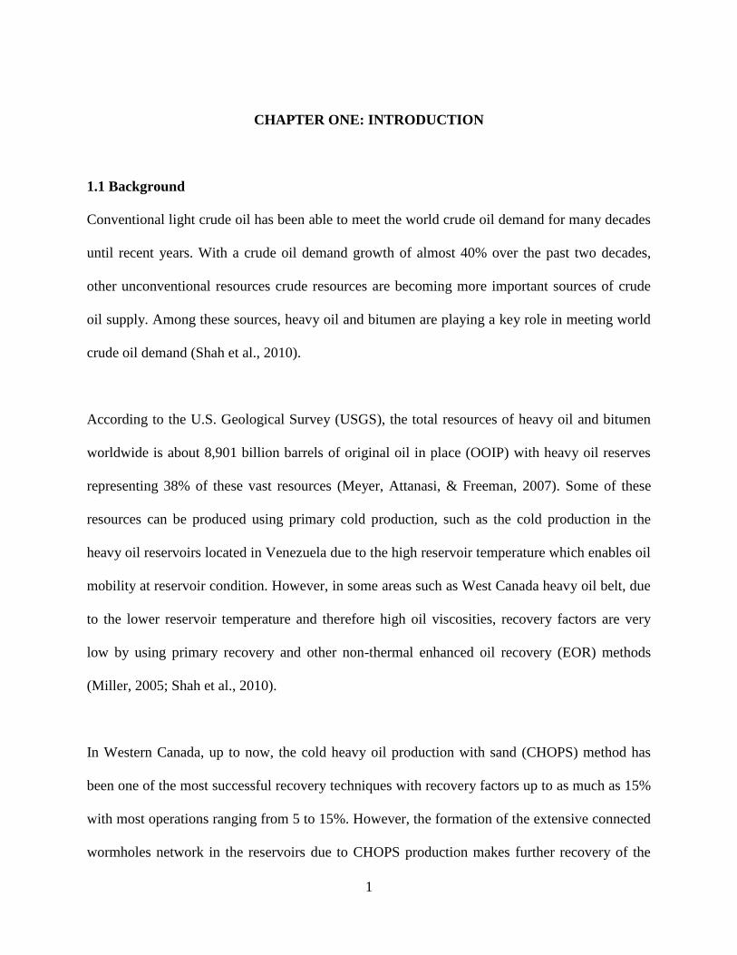
Figure 1.3 shows the temperature-dependent viscosity variations of several differential crude oil

found in Canada. While the viscosity of light crude oil can be as low as less than 10 centipoise

(cP), the bitumen in Athabasca region can be in the order of magnitude of millions cP (Gates,

2007). Biodegraded heavy oil reservoirs can also exhibits vertical variation of oil composition

and properties due to interacting factors including oil charge mixing, degradation rates, and

water and nutrient supply to the microbes. A more detailed discussion of fluid property

variations in heavy oil reservoirs can be found in a previous study (Larter et al., 2008).

4

Figure 1.3: Schematic temperature-dependent viscosity profiles of different Canadian

crude oils (modified from Meyer et al., 2007).

1.3 Heavy Oil in Canada

The heavy oil and bitumen deposits in Canada are mainly found in the province of Alberta and

Saskatchewan, shown in Figure 1.4. These heavy oil and bitumen-rich regions, Athabasca, Cold

Lake, and Peace Rivers, along with the Carbonate Triangle, cover a total area of 141, 000 km2

and contains 1.7 trillion barrels of oil OOIP which is about 25% of the total heavy oil resources

discovered worldwide. The vast amount of oil resources enables Canada to rank third worldwide

behind Venezuela and Saudi Arabia. These heavy oil reservoirs are typically found to contain

crude oil with oil viscosities up to several millions cP and typically called bitumen.

5

1.4 Geology

The Western Canadian Sedimentary Basin (WCSB), shown in Figure 1.4, is a gigantic

sedimentation basin underlying a total area of consisting of 1,400,000 km2 in Western Canada

including Northeastern British Columbia, Alberta, Southeastern Saskatchewan, Southwestern

Manitoba, and Southwestern corner of the Northwest Territories. WCSB takes a form of huge

wedge extending from Rock Mountains, which it is as thick as 6 kilometers, and thin to zero in

the east edge. WCSB contains one of the largest petroleum reserves in the world. The most oil

and gas resources, and almost all the heavy oil and bitumen resources are found in Alberta.

Figure 1.4: Tectonic setting of the western Canada Sedimentary Basin from the Late

Jurassic to the Early Eocene (courtesy of Peacock, 2009, used with permission).

6

Figure 1.5: Generalized stratigraphic column of the Western Canada Sedimentary Basin

(courtesy of Peacock, 2009, used with permission).

The heavy oil and bitumen deposits in WCSB ranges in ages from Upper Devonian to Lower

Cretaceous, as shown in Figure 1.5. A number of formations (i.e., Grand Rapids, Clearwater,

Wabiskaw, and McMurray formations) contain high quality source rocks with vast amount of

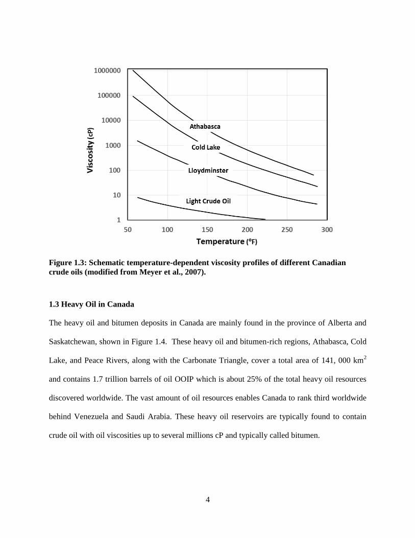
organic content and hydrogen indices. As shown in Figure 1.6, a highly efficient migration

system was developed, due to the existence of Joli Fou Shale, which serves as a top seal layer,

combined with synclinal foreland basin geometry.

7

Figure 1.6: Regional cross-section through the Western Canada Sedimentary Basin

showing location of the Athabasca heavy oil deposit (courtesy of Peacock, 2009, used with

permission).

It is suggested that oil migrated from source rocks from the Jurassic and or Mississippian periods

to the rocks from the Cretaceous period. The migration travelled a distance about 360 kilometers

to Athabasca area in millions of year. Along with the migration, fresh water meteoric recharges

from the eastern edge which led to biodegradation of the conventional components of the oil

8

which left the heavy oil and bitumen being the dominant portion of the remaining petroleum

resources. As results of the high viscosity, the oil resources are trapped and form the oil sands

reservoirs in today’s Athabasca, Peace River, and Cold Lake deposits.

1.5 Heavy Oil Production in Canada

About 20% of these bitumen resources are contained in very shallow reservoirs (less than 100

meters in depth) and can be recovered by using mining technology (Shah et al., 2010) while the

oil resources contained in deeper reservoir can only be recovered using thermally based in-situ

methods such as Steam-Assisted Gravity Drainage (SAGD) and Cyclic Steam Stimulation

(CSS). The current oil production from these unconventional techniques is estimated to be ~2.4

million barrels per day, which is 60% of total Canadian oil production of ~3.9 million barrels per

day(Canadian Association of Petroleum Producers, 2015).

The conventional heavy oil reservoirs are typically found in the Lloydminster area, located near

the border of Alberta and Saskatchewan with approximately 1.3 billion barrels of reserve. In

these reservoirs, the viscosity of the heavy oil are much lower than that of bitumen and therefore

it is feasible to extract oil using conventional primary and enhanced oil recovery methods.

Subject to reservoir conditions, two different primary recovery techniques can be used for heavy

oil production:

(1) Cold heavy oil production without sand;

(2) Cold heavy oil production with sand (CHOPS) (Dusseault & El-Sayed, 2000).

In the first method, heavy oil is produced by primarily utilizing the reservoir pressure (solution

gas drive) and sand production is prevented. However, the oil production rates are typically

9

found to be very low. In the second method, sand production is deliberately utilized to increase

the oil production rates. The current crude oil production from conventional heavy oil reservoirs

is estimated to be 423,000 barrels per day (National Energy Board, 2015) which is 11% of the

Canadian total production.

In its latest report in 2015, Canadian Association of Petroleum Producers forecasted that the total

Canadian oil production will reach 5.3 million barrel per day in 2030, with the major production

growth from oil sand projects while conventional heavy oil production is projected to gradually

decline (Canadian Association of Petroleum Producers, 2015).

1.5 Research Questions

The literature review, presented in Chapter 2, leads to the following research questions:

1. How effective is steam and hot water for recovering oil from a thin heavy oil reservoir?

2. What is the optimal hot water flooding strategy for producing thin heavy oil reservoirs?

3. How effective are solvent-aided thermal recovery processes for thin heavy oil reservoirs?

4. What injection strategy would be effective for a thin post-CHOPS heavy oil reservoir?

1.6 Outline of Thesis

This thesis is organized into six chapters and Chapter 2-7 are summarized below:

Chapter Two: This chapter provides a literature review of the heavy oil recovery techniques

and recent industry advancement for thin heavy oil reservoirs. Discussion of the mechanisms,

10

performances, and challenges of different existing recovery methods and the motivation of the

current research are included.

Chapter Three: This chapter summarizes the investigation of the performance of steam and hot

water-based recovery processes of a thin heavy oil reservoir.

Chapter Four: This chapter summarizes the efforts on optimization of hot water-flooding

strategies by using simulated annealing algorithm at different reservoir conditions.

Chapter Five: This chapter describes the research efforts to understand and design solvent-aided

thermal recovery processes for heavy oil reservoirs.

Chapter Six: This chapter summarizes the work to evaluate different oil recovery strategies as

post-CHOPS follow-up processes to raise the overall recovery factor of the reservoir.

Chapter Seven: This chapter provides a summary of the conclusion of this research work and

lists recommendations for future work based on the results discussed in this thesis.

1.7 References

Akbarzadeh, K., Hammami, A., Kharrat, A., Zhan, D., Allenso, S., Creek, J. L., Solbakken, T.

(2007). Asphaltenes—problematic but rich in potential. Oilfield Rev, 19(2), 22-43.

Canadian Association of Petroleum Producers. (2015). Crude Oil: Forcast, Markets &

Transportation.

Dusseault, M. B., & El-Sayed, S. (2000). Heavy-Oil Production Enhancement by Encouraging

Sand Production. Paper presented at the The 2000 SPE/DOE Improved Oil Recovery

Symposium Tulsa, Oklahoma.

11

Gates, I. D. (2007). Oil phase viscosity behaviour in Expanding-Solvent Steam-Assisted Gravity

Drainage. Journal of Petroleum Science and Engineering, 59, 123-134.

Istchenko, C. (2012). Well-wormhole model for CHOPS. (Master of Science), University of

Calgary.

Larter, S., Adams, J., Gates, I. D., Bennett, B., & Huang, H. (2008). The Origin, Prediction and

Impact of Oil Viscosity Heterogeneity on the Production Characteristics of Tar Sands and

Heavy Oil Reservoirs. Journal of Canadian Petroleum Technology, 47, 52-61.

Meyer, R. F., Attanasi, E. D., & Freeman, P. A. (2007). Heavy Oil and Natural Bitumen

Resources in Geological Basins of the World

Miller, K. A. (2005). State of the Art of Western Canadian Heavy Oil Water Flood Technology.

Paper presented at the The Petroleum Society’s 6th Canadian International Conference

(56th Annual Technical Meeting), Alberta, Canada.

National Energy Board. (2015). Estimated Production of Canadian Crude Oil and Equivalent

Retrieved from https://www.neb-one.gc.ca/nrg/sttstc/crdlndptrlmprdct/stt/stmtdprdctn-eng.html.

Peacock, M. J. (2009). Athabasca oil sands: reservoir characterization and its impact on thermal

and mining opportunities. Paper presented at the The 7th Petroleum Geology Conference,

London.

Shah, A., Fishwick, R., Wood, J., Leeke, G., Rigby, S., & Greaves, M. (2010). A review of novel

techniques for heavy oil and bitumen extraction and upgrading. Energy Environ. Sci., 3,

700-714.

Towson, D. E. (1997). Canada's Heavy Oil Industry: A Technological Revolution. Paper

presented at the The 1997 SPE International Thermal Operations and Heavy Oil

Symposium, Bakersfield, CA.

https://www.neb-one.gc.ca/nrg/sttstc/crdlndptrlmprdct/stt/stmtdprdctn-eng.html

12

CHAPTER TWO: REVIEW OF LITERATURE

2.1 Background

It is estimated that about 80% of 170 billion barrels of technically recoverable heavy oil and

bitumen resources in Canada cannot be recovered by mining and have to be exploited by using

other in situ techniques example being various in situ methods including such as the Cyclic

Steam Stimulation (CSS) and Steam-Assisted Gravity Drainage (SAGD) techniques. The most

widely used recovery technologies, although commercially successfully, are all known for their

advantages and disadvantages on technical and or socio-economic aspects.

Up to date, mining technology for bitumen are relative mature but is well known for its adverse

impact on environment such as disturbing larges areas of muskeg and forest and creating

significant water pollution. In situ methods such as SAGD techniques, avoids has lower surface

disturbance but requires large amounts of water and generates significant greenhouse gas

emission due to steam generation. Therefore there is an eminent need for technological

advancements in heavy oil and bitumen recovery methods which can make recovery of the vast

heavy oil and bitumen resources more economic and environmentally benign.

In this chapter, we will review different technologies commercially utilized for heavy oil and

bitumen recovery in terms of mechanisms and current applications with focus on:

Non-thermal methods including primary production with or without sands and different

enhanced oil recovery techniques;

Thermally based technologies such as steam and hot water flooding, Cyclic Steam

13

Stimulation (CSS), Steam Assisted Gravity drainage (SAGD);

Solvent-aided/based recovery technologies including ES-SAGD and VAPEX;

Enhanced oil recovery methods after primary recovery.

We will also discuss the applications of these techniques to heavy oil resources with focus on

thin heavy oil reservoir. In the end, a discussion will be given to the motivation of the present

study.

2.2 Primary heavy oil production

2.2.1 Heavy Oil Production without Sand

In reservoirs where heavy oil viscosity is sufficiently low at reservoir conditions, the heavy oil is

sufficiently mobile so that they can be produced by primary cold production. In the Orinoco

heavy-oil belt in Venezuela, much of the oils are produced in this way. The heavy oil resources

in western Canada are found in Northeastern Alberta and western Saskatchewan. In these

regions, primary cold production is the most common way to extract the heavy oil resources.

However, the heavy oil reservoirs are often found to have low reservoir temperature, solution gas

content, and bottom water. Therefore one typical problem for heavy oil primary production by

using vertical wells is the tendency for water to cone up from an underlying aquifer (Towson ,

(1997). As a result, the recovery factors are low, and typically found to be around 3-5%.

With development of high precision horizontal well drilling technology, more heavy oil

production has been realized by using horizontal wells. Compared with vertical wells, the

horizontal wells, with well length as long as 1,500 meters, enables much larger drainage volume

and production rates. At the same time, because of much larger wellbore contact with reservoir,

14

a horizontal well usually has a lower pressure drawdown for a given productivity compared with

a vertical well and therefore the tendency for water to cone up is less (Towson , (1997).

2.2.2 Cold Heavy Oil Production with Sand (CHOPS)

In western Canada, the heavy oil resources are usually found in reservoirs with high permeability

and unconsolidated sandstones. Often the oil production is accompanied with sand productions.

Initially in the early years, sand production was purposely limited and prevented (Geilikman et

al., 1994). However it was revealed later that encouraging sand production could lead to

increased oil production. With the development of progressive cavity pumps (PCPs), a new

heavy oil production technology, called Cold Heavy Oil Production with Sand (CHOPS),

emerged. By converting the conventional heavy oil wells to CHOPS wells where the sand

production is aggressively encouraged, the improved oil production can be 10 times higher than

their original production rates. At the same time, recovery factors are higher – around 10% or up

to 15% in some cases.

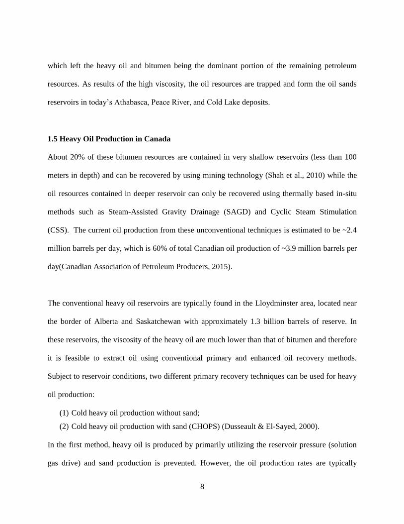
Figure 2.1: Illustration of top view of a wormhole zone. The center spot represents the

wellbore (modified from Yuan et al., 1999).

15

However, one significant problem with CHOPS is the formation of extensively connected

wormhole network in the reservoir with zones adjacent to the network depleted of reservoir

pressure. The wormholes and their associated network are believed to be channels with diameters

of the order of tens of centimeters and extending tens up to a few hundred meters within the

reservoir. In many cases, it has been observed that wormhole networks are connected to other

wormhole networks with long distance apart. It was shown by fluorescein dye tracer tests

(Squires, 1993) that communication between well in post-CHOPS field can occur with speeds of

up to about 400 m/h, which clearly indicated existing connections between wormhole networks.

Another study (Yeung, 1995) by using tracer tests for a producing CHOPS field demonstrated

that the fluorescein dye injected into one well can be produced from neighboring wells within a

few hours although they are up to 500 meter apart.

The creation of wormhole networks and depletion of reservoir pressure driven by the CHOPS

process present severe challenges for applying follow-up processes to recover additional oil after

CHOPS operations. Moreover, if the wormhole networks get connected with aquifer, the

significant water production will quickly force abandonment of the CHOPS process and make

further follow-up oil recovery very challenging.

2.3 Thermally based heavy oil recovery methods

2.3.1 Steam Flooding and Hot Water Flooding

Steam flooding is a process in which high pressure steam is injected into the oil zone to supply

the thermal energy to reduce the viscosity of oil which will be pushed towards to production well

16

under pressure gradient, as shown in Figure 2.2. It is suggested (Farouq Ali, 1974) that steam

flooding methods can be applied to heavy oil reservoirs with crudes in the range 12º – 25 º API.

Figure 2.2: Illustrative mechanism of steam flooding process.

In a steam flooding process, the steam is primarily used as displacing agent which is intended to

displace the oil in place. To make steam flooding effective, the oil viscosity at reservoir

conditions should be low enough to provide mobility, along with a high permeability of the

reservoirs. As shown in Figure 2.2, there is a steam zone in the vicinity of the injection well at

steam temperature. Further ahead, there is hot water zone in which mixture of heated oil and hot

water is pushed ahead towards production wells. In practice, there is a tendency for injected

steam to segregate to the upper zone of the oil layer. So the heat loss for thin heavy oil reservoirs

typically very significant.

17

In a hot water flooding case, hot water is injected into the oil zone as displacing agent. Compared

with steam flooding, water flooding has advantages under special circumstances. For deep

reservoirs with enough oil mobility, hot water flooding can provide the required high pressure at

lower energy requirements due to low heat loss. However, there are also disadvantages for a hot

water flooding process. A major problem is the severe viscous fingering of the injected hot water

due to high mobility of the water and low mobility of the in-place oil, which can result in poor

volumetric sweep efficiency and early water breakthrough (Farouq Ali, 1974).

2.3.2 Cyclic Steam Stimulation

Cyclic Steam Stimulation (CSS) was initially investigated by Shell for its heavy oil reservoirs in

Venezuela (Shah et al., 2010). CSS is three-stage process, as illustrated in Figure 2.3. In the first

stage, high-pressure steam is injected into the pay zone is deliver the thermal energy to mobilize

the oil and build up reservoir pressure. The steam injection period could last for up to a month. In

the second stage, also called soak stage, the well is shut in to allow distribution of injected heat

to the reservoir. After the soak stage, the well is put on production. The initial production rates

are typically very high for short period of time and then decline gradually over several months.

After depletion of reservoir pressure which results in very low production rate, further

production is no longer economic, the well will be put on steam injection stage again and the

whole process repeats for another injection-soak-production cycle.

Due to the high initial production rates, CSS processes typically have short payback periods. At

later stage, due to the higher steam-oil-ratio, the CSS processes are typically converted into

steam flooding processes (Shah et al., 2010).

18

Figure 2.3: Illustration of Cyclic Steam Stimulation (CSS) process (Borberg and Lantz,

1966).

CSS method is essentially a formation stimulation process and recovery factors are low – very

often found to be in the range of 10-15% of the oil-in-place. For thin heavy oil reservoirs,

however, no commercial success has been reported, due to the excess heat loss which makes the

soak ineffective.

2.3.3 Steam Assisted Gravity Drainage

The Steam-Assisted Gravity Drainage (SAGD) process was developed by Butler when he was

working for Imperial Oil for in situ bitumen recovery (Butler, 1985). In a typical SAGD process,

two horizontal wells, which are parallel to each other with approximately 5 meters apart, are

employed, with one used as steam injection well and the other one used as production well, as

showed in Figure 2.4.

19

To make a SAGD process successful, a steam circulation process for both the injection and

production wells, in a period of about three months, is required to establish the communication

between injection and production wells. After the establishment of effective inter-well

communication, steam is then continuously injected into the reservoir though injection well to

form a steam chamber. As illustrated in Figure 2.4, the heated bitumen and condensate will flow

along the edge of the steam chamber downward into the liquid pool, which will effectively

prevent direct production of injected steam.

Figure 2.4: Illustration of the steam chamber cross-section in SAGD process (Gates and

Leskiw 2008, used with permission).

Up to date, SAGD method has been one of the most successful bitumen recovery techniques in

western Canada (Gates, 2011; Shah et al., 2010).

20

As another version of SAGD, the cross SAGD (Stalder, 2009) was proposed by Stalder as a

novel bitumen recovery method in which the horizontal oil production wells are placed

perpendicular to the injection wells. With a mechanism combining gravity drainage and lateral

displacement, the XSAGD method is suggested that it could realize better economics for thin pay

reservoirs although at the expense of lower recovery factor.

However, for successful applications of SAGD processes, there are requirements such as

presence of effective cap-rock, high vertical permeability, good reservoir geological properties,

pay zone thickness and others. It is especially challenging to apply SAGD method to thin heavy

oil reservoirs due to the small reservoir pay zone thickness (e.g., less than 6 meters) which makes

effective vertical separation of the injection and production well very difficult. Moreover, with a

small reservoir thickness, the steam chamber will quickly reach the top the pay zone and incur

excess heat loss to over-burden. Therefore, up to date, for heavy oil and bitumen reservoirs with

pay zone less than 10 meters, SAGD methods are not considered to be economic.

2.4 Solvent-aided/based recovery technologies

2.4.1 ES-SAGD

In heavy oil and bitumen recovery processes, the key is to reduce the oil viscosity to provide

enough mobility for the oil to be extracted. In SAGD process, thermal energy is delivered to the

reservoir to reduce the oil viscosity to enable the gravity drainage mechanism to work. Besides

thermal energy, there are also alternative processes to improve the oil phase mobility. One

example is the adding of solvents to the heavy oil and bitumen phase. Figure 2.5 shows the

viscosity of mixture of Athabasca bitumen and hexane at different temperatures. It can be seen

21

clearly the bitumen viscosity can be effectively reduced by adding solvents without changes in

temperature.

For some solvents, for example, propane, the bitumen phase viscosity can be further reduced due

to the precipitation of asphaltenes from the bitumen. Therefore, in a thermal oil recovery process,

sufficient mobility of bitumen can be achieved by adding solvent while keep temperature

relatively lower.

Figure 2.5: Viscosity of mixtures of Athabasca bitumen and hexane as calculated from

Shu's (1984) correlation (Gates, 2007, used with permission).

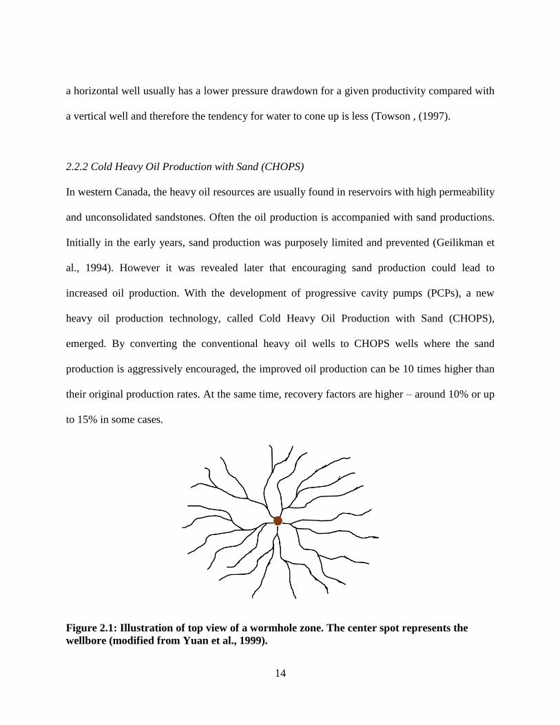
In the Expanding-Solvent Steam-Assisted Gravity Drainage (ES-SAGD) process (Nasr & Isaacs,

2001) which is essentially an enhanced SAGD process, a small amount of solvent is added to the

injected steam to thermal efficiency. As shown in Figure 2.6, a mixture of steam and solvent is

22

injected into the steam/solvent chamber and condense at the edge of the chamber. On one hand,

thermal energy is delivered to the bitumen by release of latent heat of steam. On the other hand,

solvent diffuses into the bitumen phase and further reduce its viscosity.

Figure 2.6: Cross-section of the Expanding-Solvent Steam-Assisted Gravity Drainage (ES-

SAGD) process (Gates, 2007, used with permission).

Due to the fact that bitumen viscosity can be reduced to achieve the targeted mobility with less

consumption of thermal energy compared with a steam-only SAGD process, the thermal loss to

over-burden and under-strata is greatly reduced. There is also one major disadvantage to use ES-

SAGD process which is the solvent retention in the reservoirs. Since solvents are more expensive

than bitumen, it is therefore critical to ensure a high recovery of the solvent injected. Similar to

SAGD process, it is challenging to apply ES-SAGD process to thin heavy reservoirs. Although

the heat efficiency is improved, but how to recover the solvent injected can be difficult due to

factors such as geological heterogeneities.

23

2.4.2 VAPEX method

For thin heavy oil reservoirs typically found in Northeastern Alberta and Southwest

Saskatchewan, up to date, it has been challenging to apply thermally-base techniques due to

excess heat loss. To address this problem, a solvent based Vapor Extraction (VAPEX) method

has been proposed and investigated for heavy oil and bitumen recovery (Allen, 1978; Butler,

1997).

In the VAPEX process, a mixture of solvent vapor is injected into the reservoir through a

horizontal injection well located in the upper oil zone and forms a solvent vapor chamber. With

effective mixing of the bitumen and solvent at the edge of the chamber, the bitumen viscosity is

significantly reduced and mobilized bitumen flows towards the lower production well under

gravitational force along the edge of the solvent vapor chamber. The solvents are carefully

chosen (e.g. ethane, propane, butane, etc.) to that they can form a vapor phase without additional

heat at reservoir conditions. The injected solvent is dissolved into the bitumen by diffusion to

reduce the oil viscosity and mobilize the oil. Due to absence of heat loss to over-burden and

under-strata, the VAPEX is suggested to be a more economic process, especially for thin heavy

oil reservoirs (Butler and Mokrys, 1991).

However, there are also disadvantages with VAPEX method. For instance, compared with

SAGD process, production rates of VAPEX process are lower due to the relative slow diffusion-

based mixture process. In addition, the high cost of solvent cost is a major concern and how to

ensure a high recovery of solvents is still a challenge to overcome.

24

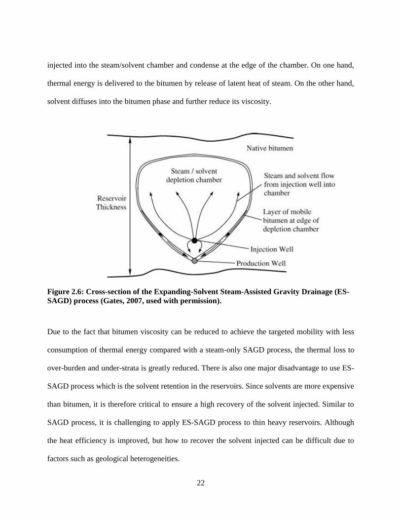
There have been efforts in making VAPEX a more efficient heavy oil recovery method. Butler

proposed that hot water can be injected along with the solvent vapor. As illustrated in Figure 2.7.

The injection of hot water enables distribution of heat laterally away from injection well to

reservoir. The temperature and injection rates of hot water are controlled to raise the reservoir

temperature to a range from 40 – 80º C. The rise in reservoir temperature is only modest so that

excess heat loss is prevented.

Figure 2.7: Illustration of solvent vapor chamber in VAPEX process (modified from Butler

and Mokrys, 1991).

However, up to date, success of VAPEX in laboratories has not been transferred into applications

of VAPEX in commercial projects. This is possibly due to the low drainage rates and high

solvent to oil ratio which are not promising enough to ensure the VAPEX to be economically

viable.

25

2.5 Enhanced oil recovery after primary recovery

2.5.1 Water Alternating Gas (WAG) process

Water alternating gas injection (WAG) is an enhanced recovery process involving drainage and

imbibition taking place in cyclic alternation or simultaneously in the reservoir (Nezhad et al.,

2006). The first application of WAG process was reported for the North Pembina Field in

Alberta in 1957 (Christensen et al., 2001). Since then it has been widely used as an effective

EOR technique. The WAG injection was initially proposed to improve the sweep efficiency of

gas injection by utilizing the injected water to control the displacement and front, as illustrated in

Figure 2.8. At microscopic level, the displacement of the oil by gas is more effective than by

water. However, at macroscopic level, due to its low viscosity and therefore high mobility, gas-

alone flooding typically results in quick breakthrough and poor sweep efficiencies. By using both

water and gas injection, WAG techniques can achieve both macroscopic sweep efficiency of

water flooding and the high displacement efficiency of gas injection to realize incremental oil

production (Kulkarni & Rao, 2005).

26

Figure 2.8: Schematic representation of WAG injection.

There are also other enhanced oil recovery processes involving use of gas and water injection

with example being Methane Pressure-Cycling (MPC) process (Dong et al,, 2006). The essence

of the MPC process is to restore the solution-gas-drive mechanism. By injection of solution gas

(e.g. methane) along with water injection, the initial reservoir pressure can be restored. The

injected gas contacts and dissolves into the remaining oil in the reservoir to enable further oil

production under a re-energized solution-gas-drive mechanism. Due to the low energy cost of

this process, it have been suggested to be an effective technique for enhanced oil recovery for

thin heavy oil reservoirs after primary production (Dong et al., 2006).

27

2.5.2 Cyclic Solvent Injection (CSI) process

It is known that CHOPS can only extract 10-15% of original oil in place (OOIP) for heavy oil

reservoirs. There have been investigations on follow-up process on how to recover the remaining

oil and cyclic solvent injection (CSI) has been one of these efforts (Ivory et al., 2010).

The mechanism of the CSI process is similar to that of the cyclic steam stimulation (CSS)

process. In a CSI process, a gas solvent (close to the dew point) is first injected for a period of

time until the pressure is close to the initial reservoir pressure. The solvent used should have a

high solubility in the oil to enable oil swelling and viscosity reduction and solution-gas-drive

mechanism, but stay in the gas phase to pressurize the reservoir without excess requirement of

solvents (Chang et al., 2014). After the injection period, the solvents are allowed to further

diffuse into the oil phase, a process also known as soaking, before well is put on production to

extract the oil until reservoir pressure depletes again, as illustrated in Figure 2.9.

Figure 2.9: Schematic of CSI well during injection (left) and production (right) (modified

from Ivory et al., 2010).

28

In a previous field study as part of the $40 million Joint Implementation of Vapor Extraction

Program (JIVE), the CSI process was shown to be able to realize significant incremental oil

recovery for thin Lloydminster heavy oil reservoir with wormholes (Chang et al., 2014). By

using detailed reservoir simulation approach, Istchenko (Istchenko, 2012) evaluated the

performance of different solvent composition used in CSI process as a follow-up process of a

post-CHOPS reservoir. The results indicated a promising energy efficiency which is higher than

that of a pure thermal process.

There are also other enhanced oil recovery techniques in situ combustion (Chen J, 2012), CO2

flooding (Derakhshanfar et al., 2012; Nasehi and Asghari, 2012; Istchenko, 2012), and chemical

flooding (Krumrine et al., 2014), and many others. Further review of these technological

explorations is beyond the scope of the present study.

2.6 Research Objectives

The objectives of the present study research documented here is to develop effective oil recovery

strategies and processes for both unexploited and post-CHOPS thin heavy oil reservoirs. By

investigating and understanding the mechanism of different proposed oil recovery processes, we

aim to design effective strategies that are both economic and environmentally benign. In the

research documented in this thesis, the research has been focused on different thermally-based

processes and the impact of addition of solvent.

29

2.7 References

Allen, J. C. (1978). Canada Patent No. 1027851.

Boberg, T.C. and Lantz, R.B. (1966). Calculation of the Production Rate of a Thermally

Stimulated Well. Journal of Petroleum Technology, 18, 1613–1623.

Butler, R., & Mokrys, I. (1991). A New Process (VAPEX) For Recovering Heavy Oils Using

Hot Water And Hydrocarbon Vapour. Journal of Canadian Petroleum Technology,

30(1), 97-106.

Butler, R. M. (1985). A New Approach To The Modelling Of Steam-Assisted Gravity Drainage.

Journal of Canadian Petroleum Technology, 24, 42-50.

BUTLER, R. M. (1997). United States Patent No. 5,607,016.

Chang, J., Ivory, J., & Beaulieu, G. (2014). Pressure Maintenance at post-CHOPS Cyclic

Solvent Injection (CSI) Well Using Gas Injection at Offset Well. Paper presented at the

The SPE Heavy Oil Conference-Canada, Calgary, Alberta.

Chen J, C. R., Oldakowski K, Wiwchar B. (2012). In situ combustion as a followup process to

CHOPS. Paper presented at the The SPE Heavy Oil Conference Canada,, Calgary,

Alberta, Canada.

Christensen, J. R., Stenby, E. H., & Skauge, A. (2001). Review of WAG Field Experience. SPE

Reservoir Evaluation & Engineering, 4(2), 97-106.

Derakhshanfar, M., Nasehi, M., & Asghari, K. (2012). Simulation study of CO2-assisted

waterflooding for enhanced heavy oil recovery and geological Storage Paper presented at

the The Carbon Management Technology Conference, Orlando, Florida.

Dong, M., Huang, S.-S., & Hutchence, K. (2006). Methane Pressure-Cycling Process With

Horizontal Wells for Thin Heavy-Oil Reservoirs. SPE Reservoir Evaluation &

Engineering, 9(2), 154-164.

Farouq Ali, S. M. (1974). Heavy Oil Recovery – Principles, Practicality, Potential, and

Problems. Paper presented at the The Rocky Mountain Regional Meeting, Billings,

Montana, USA.



Gates, I. D. (2011). Basic Reservoir Engineering (1st ed.): Kendall Hunt.

Gates, I. D., & Leskiw, C. (2008). Impact of Steam Trap Control on Performance of Steam-

Assisted Gravity Drainage Paper presented at the The Canadian International Petroleum

Conference/SPE Gas Technology Symposium 2008 Joint Conference (the Petroleum

Society’s 59th Annual Technical Meeting), Calgary, Alberta, Canada.


Calgary.

Ivory, J., Chang, J., Coates, R., & Forshner, K. (2010). Investigation of cyclic solvent injection

process for heavy oil recovery. Journal of Canadian Petroleum Technology, 48, 22-33.

Geilikman, M.B., Dusseault, M.B. and Dullien, F.A.: “Fluid Production Enhancement by

Exploiting Sand Production,” presented at SPE/DOE Improved Oil Recovery

Symposium, Tulsa, Oklahoma, SPE 27797, 17-20 April, 1994.

Krumrine, P. H., Lefenfeld, M., & Romney, G. A. (2014). Investigation of Post CHOPS

Enhanced Oil Recovery of Alkali Metal Silicide Technology. Paper presented at the The

SPE Heavy Oil Conference-Canada, Calgary, Alberta, Canada.

30

Kulkarni, M. M., & Rao, D. N. (2005). Experimental investigation of miscible and immiscible

Water-Alternating-Gas (WAG) process performance. Journal of Petroleum Science and


Nasr, T. and Isaacs, E. (2001). Process For Enhancing Hydrocarbon Mobility Using a Steam

Additive, U.S. Patent 6230814.

Nezhad, S., Mojarad, M., Paitakhti, S., Moghadas, J., & Farahmand, D. (2006). Experimental

Study on Applicability of Water.Alternating-CO2 injection in the Secondary and Tertiary

Recovery. Paper presented at the The First International Oil Conference and Exhibition in

Mexico, Cancun, Mexico.



London.



700-714.

Shu, W. R. (1984). A viscosity correlation for mixtures of heavy oil, bitumen, and petroleum

fractions. Soc. Pet. Eng. J., 24(3), 277-282.

Squires, A. (1993). Inter-well tracer results and gel blocking program. Paper presented at the

The 10th Annual Heavy Oil and Oil Sands Technical Symposium, Calgary, Alberta,

Canada.

Stalder, J. L. (2009). Unlocking Bitumen in Thin and/or Lower Pressure Pay Using Cross SAGD

(XSAGD). Journal of Canadian Petroleum Technology, 48, 34-39.




Yeung, K. (1995). Cold production of crude bitumen at the Burnt Lake Project, Northeastern

Alberta, Canada. Paper presented at the The 6th UNITAR International Conference on

Heavy Crude and Tar Sands, Houston, Texas.

Yuan, J.-Y., Tremblay, B., & Babchin, A. (1999). A Wormhole Network Model of Cold

Production in Heavy Oil. Paper presented at the The 1999 SPE International Thermal

Operations

and Heavy Oil Symposium, Bakersfield, California.

31

CHAPTER THREE: THERMAL RECOVERY STRATEGIES FOR THIN HEAVY OIL

RESERVOIRS

This chapter was published in the peer-reviewed journal Fuel (2014 impact factor 3.52). The

citation is as follows: Zhao, W., Wang, J., and Gates, I.D. “Thermal Recovery Strategies for

Thin Heavy Oil Reservoirs,” Fuel, vol. 117, pp. 431–441, 2014.

3.1 Abstract

Up to 80% of heavy oil reservoirs in Western Canada are less than 5 m thick and as yet the only

economic processes are cold production ones which realize recovery factors between 10% and

15%. This implies that >85% of the oil remains in the ground after the process becomes

uneconomic to continue operation. At this time, no thermal processes exist that are economic.

Here, a reservoir simulation study was conducted to guide the design of thermal recovery

processes for a heavy oil reservoir with a thickness of 4 m by comparing different operating

strategies including Steam-Assisted Gravity Drainage (SAGD), steam flooding, hot water

flooding, and alternating steam/hot water flooding. A base case of cold production (without

sand) was also done for comparison purposes. It was found that the cold production case was not

viable with very low recovery factor. Higher recovery factor was achieved by using SAGD

strategy but at a poorer thermal efficiency. Steam flooding operations exhibits better

performance than SAGD in terms of heat utilization. However, its high heat loss to the over and

underburden leads to higher cumulative-energy-injected-to-oil ratio (cEOR). Hot water flooding,

however, achieved oil production rates comparable to steam flooding at much lower cEOR. The

flood cases are tested at different well separations. However, the results suggest that hot water

32

flooding alone may not be the target process of choice for thin heavy oil reservoirs and solvents

may be needed to lower the energy intensity further.

3.2 Introduction

About 80% of heavy oil resources in Western Canada are found in reservoirs less than 5 m thick

(Adams, 1982). These reservoirs typically have relatively high permeability (often between 1 and

5 Darcy) with oil viscosities between 1000 and 35,000 cP. Under typical cold production

conditions without sand production, the average recovery factor is typically between 3% and 8%

of the original oil in place (Adams, 1982). If there is sufficient solution gas and the formation is

unconsolidated, then these reservoirs are typically produced by Cold Heavy Oil Production with

Sand (CHOPS) methods but these approaches tend to recovery less than 15% of the oil within

the reservoir before they become uneconomic (Pan et al., 2010). Also, the formation of

wormholes during CHOPS operation often presents difficulties for applying follow-up processes

to increase the recovery factor beyond that of CHOPS (Shah et al., 2010). Recovery processes

that realize larger recovery factor and remain energy efficient (so they remain economic) are

needed for these thin reservoirs. In general, current thermal-based techniques such as Steam-

Assisted Gravity Drainage (SAGD) and Cyclic Steam Stimulation (CSS) for recovering oil from

thin heavy oil (<10 m) reservoirs are considered not viable recovery processes due to significant

heat losses to understrata and overburden. In SAGD and CSS in thin reservoirs, the energy

efficiency of the processes is expected to be low: the invested (injected) energy per unit realized

energy (in the form of oil) renders the processes uneconomic. As yet, there are no studies that

have reported on the performance of SAGD and CSS in reservoirs with oil column thickness <5

m.

33

In conventional oil reservoirs, water flooding has been the most widely used techniques for

secondary recovery after the end of primary production (Miller, 2005). For heavy oil reservoirs,

however, the performance of water flooding strategy is much poorer and limited successful cases

are mostly found for reservoirs with dead oil viscosity below 1000–2000 cP (Miller, 2005). The

poor sweep efficiency is caused by the adverse oil–water mobility ratio, reservoir heterogeneity,

and high oil viscosity after primary production due to depletion of solution gas, and so on.

Adams (Adams, 1982) reported that the incremental oil recovery from water flooding typically

was found to be no more than 1–2% in the Lloydminster area of Western Canada.

Polymer flooding techniques have been widely used as enhanced oil recovery approaches after

water flooding (Asghari & Nakutnyym, 2008). The purpose of injecting polymer solution is to

improve the mobility ratio between the injectant and oil to reduce water fingering therefore

leading to additional oil recovery. Canadian Natural Resources Ltd. has been adopting this

strategy in the Pelican Lake area and reported a total oil recovery factor up to 17% with

application of polymer flooding techniques (Canadian Natural Resources Ltd., 2011). The use of

polymer flooding or other secondary oil recovery techniques such as alkaline/surfactants

flooding (Dong et al., 2009) and (Jamaloei et al., 2012) has been limited to reservoirs with a dead

oil viscosity in the order of few thousands of centipoise (Asghari and Nakutnyym, 2008; Gao,

2011). Even the recovery factor is greater than that achieved by cold production, over 80% of the

oil remains in the reservoir.

34

Thermal-based recovery processes for thin heavy oil were found to be rare, either in field

operations or laboratory or reservoir simulation studies. Stalder (2009) reported on reservoir

simulation results on the application of Cross SAGD (XSAGD) for a bitumen reservoir with a

net pay of 10 m. The results demonstrated that there are economic advantages of XSAGD over

traditional SAGD methods. However, he stated that it is not economic to apply XSAGD to

thinner reservoirs. Gates (2010) proposed a solvent-aided thermal recovery process for 8 m thick

oil sands reservoir. Compared with traditional SAGD, the solvent-aided process led to

substantially lower steam usage and net injected energy (both steam and solvent lost to the

reservoir) to oil ratio. Tavallali et al. reported an optimization of the SAGD well configuration

for a 10 m thick Lloydminster-type heavy oil reservoir with a dead oil viscosity of 5,000 cP

(Tavallali et al., 2012). They suggested that lateral placement of the production well is the

optimum well configuration for depleting the reservoir in the shortest period of time. To our best

knowledge, studies to understand and design thermal-based recovery processes for reservoirs

with thickness less than 5 m have not been done before.

Here, to better understand and to derive viable thermal recovery process designs for extracting

oil from thin (<5 m) heavy oil reservoirs, a reservoir simulation study has been done to

investigate steam and hot water-based recovery processes.

3.3 Reservoir Simulation Model

As shown in Figure 3.1, three general well configurations were examined: the first is cold

production by using a single horizontal well, the second is a standard Steam-Assisted Gravity

Drainage (SAGD) well-pair configuration, and the third is a linear hot water or steam-flooding

35

configuration (using two horizontal wells). For the hot water and steam-flooding operating

strategies, six inter-well spacings were evaluated (30, 40, 50, 60, 70, and 80 m). The thickness of

the heavy oil interval is equal to 4 m thick. The models were discretized into a regular Cartesian

grid with dimensions 1 m in the cross-well direction, 50 m in the downwell direction and 0.4 m

in the vertical direction. The length of the perforated sections of the horizontal wells in all

models is equal to 1,200 m. The spatial distributions of porosity (average equal to 0.32 horizontal

permeability (average equal to 3,650 mD), and oil/water saturations (average oil saturation equal

to 0.65), displayed in Figure 3.2, were derived from core data taken from the Devon heavy oil

field located in eastern Alberta. The vertical-to-horizontal permeability ratio is equal to 0.8. To

populate the spatial distributions of these reservoir properties between wells, linear random

deviations from the mean values of the properties, with properties listed in Table 3.1, were used.

The initial reservoir pressure and temperature are equal to 2,800 kPa and 20 °C. The solution

gas-to-oil ratio at original reservoir conditions is equal to 6.17 m3/m

3.

Figure 3.1: Well configurations investigated in the present study. In all the cases, the

injecting wells and producing wells are 0.6 meter above the reservoir bottom with an

exception in the SAGD case, where the injecting well is 0.6 meter below the reservoir top.

36

Table 3.1: Reservoir simulation model properties.

Property Value

Depth to reservoir top (m) 334

Net pay (m) 4

Porosity 0.32±0.02 Oil saturation 0.65±0.09

Solution gas-to-oil ratio (m3/m3) 6.17

Horizontal rock permeability kh (mD) 3,650±347 kv/kh 0.8

Effective rock compressibility (1/kPa) 14x10-6 Rock heat capacity (kJ/moC) 2,600

Rock thermal conductivity (kJ/m day oC) 660

Reference pressure (kPa) 2,800 Reference depth (m) 334

Initial reservoir temperature 20

Dead oil viscosity (cP) 20oC

40oC

80oC 160oC

250oC

15,212

1884

125.4 9.66

3.09

Water thermal conductivity (kJ/m day oC) 53.5 Gas thermal conductivity (kJ/m day oC) 5

Oil thermal conductivity (kJ/m day oC) 11.5

Methane solubility K-value correlation Kv1 (kPa) 504,547 K-value = (Kv1/P) exp(kv4/(T+Kv5)) Kv4 (

oC) -879.84

5 (oC) -265.99

Oil-water relative permeability curves Sw krw krow

0.1500 0.0000 0.9920

0.2000 0.0002 0.9790

0.2500 0.0016 0.9500

0.3000 0.0055 0.7200

0.3500 0.0130 0.6000

0.4000 0.0254 0.4700

0.4500 0.0440 0.3500

0.5000 0.0698 0.2400

0.5500 0.1040 0.1650

0.6000 0.1480 0.1100

0.6500 0.2040 0.0700

0.7000 0.2710 0.0400

0.7500 0.3520 0.0150

0.8000 0.4470 0.0000

0.8500 0.5590 0.0000

0.9000 0.6870 0.0000

0.9500 0.8340 0.0000

1.0000 1.0000 0.0000

Gas-Liquid relative permeability curves Sl krg krog

0.1500 1.0000 0.0000

0.2000 0.9500 0.0002

0.2500 0.8400 0.0016

0.3000 0.7200 0.0055

0.3500 0.6000 0.0130

0.4000 0.4700 0.0254

0.4500 0.3500 0.0440

0.5000 0.2400 0.0698

0.5500 0.1650 0.1040

0.6000 0.0930 0.1480

0.6500 0.0750 0.2040

0.7000 0.0450 0.2710

0.7500 0.0270 0.3520

0.8000 0.0200 0.4470

0.8500 0.0100 0.5590

0.9000 0.0050 0.6870

0.9500 0.0000 0.8340

1.0000 0.0000 0.9920

37

(a) oil saturation

(b) porosity

(c) horizontal permeability (in mD)

Figure 3.2: Reservoir properties of a reservoir model with a width of 40 m. The cross-

sections were taken perpendicular to the wells at the heel of the well.

A commercial thermal reservoir simulator, CMG STARS™ (CMG, 2012), was used for all

reservoir simulation models. This thermal reservoir simulator solves the material and energy

balances for multiphase (aqueous, oil, and gas) flow in porous media with convective diffusive

transport of solution gas between the oil and gas phases. Thermodynamic equilibrium, calculated

by using K-values, is imposed at each time step. The simulator uses the finite element method to

solve the governing equations (Reddy, 2005). All reservoir models were run in parallel on a quad

38

core (3.33 GHz) computer and each case took 5–8 h to complete depending on the model sizes.

The material and energy balance tolerances were set to be equal to less than 0.01%.

3.4 Details of Well Placements and Operating Strategy

3.4.1 Cold Production (Without Sand)

In this case, a single production well is placed in the reservoir. The production well is located 0.6

m above the base of the oil column. In the cross-well direction, the width of the model is equal to

101 m. This implies that the well is part of a larger pattern with 101 m spacing (symmetry

boundary conditions apply at the model side boundaries). Here, we have taken the case where

sand production does not occur, that is, the well is equipped with sand control so that oil flows

from the reservoir under volumetric expansion and solution–gas drive.

3.4.2 Steam Assisted Gravity Drainage (SAGD)

The steam-injection well is positioned 0.6 m below the caprock whereas the producer is located

0.6 above the under-burden, which gives a vertical interwell separation equal to 2.8 m. The width

of the model is equal to 101 m. Similar to the cold production model, this implies that the

wellpair is part of a larger pattern with 101 m spacing (symmetry boundary conditions apply at

the model side boundaries). For the steam injection well, the injection pressure was set equal to

4000 kPa (corresponding saturation temperature is equal to 250.4 °C) with steam quality equal to

0.9. For the production well, to impose steam-strap control, the maximum steam production rate

was constrained to 2 m3/day. Prior to SAGD operation, a 2-month preheating period is employed

to initialize the thermal communication between the injection and production wells.

39

3.4.3 Case 3. Steam Flooding

Six spacings between the injection and production wells were studied: 30, 40, 50, 60 and 80 m.

Symmetry boundary conditions are applied at the side boundaries thus these cases are

geometrically periodic. The injection pressure of steam is set equal to 4000 kPa with steam

quality of 0.9. The production wells were operated with a bottom hole pressure equal to 500 kPa.

3.4.4 Hot Water Flooding

The well configurations were the same as that used in the steam-flooding cases except hot water

was used (steam quality equal to zero).

3.4.5 Alternating Steam and Hot Water Flooding

In these cases, the same well configuration is used as that in the steam and hot water flooding

cases above except that the injection and production wells are alternated: at a specified point of

time, the injection well is converted to a production well and the production well is converted to

an injection well.

3.5 Results and Discussion

3.5.1 Cold Production (Without Sand)

A summary of the results of the cold production case is listed in Table 2. As shown in Figure 3.3,

the oil rate started at about 18 m3/day but declined rapidly below 1 m

3/day within 31 days of

production. The cumulative oil was found to be equal to 204 m3 after one year of operation and

406 m3 after 5 years of production which corresponds to a 5-year oil recovery factor equal to

0.5%. This low oil recovery is due to poor oil mobility – the average water saturation is equal to

35% and thus the relative permeability to oil is low at original reservoir conditions, the live oil

viscosity is equal to about 8917 cP (dead oil viscosity is 15,212 cP). The low oil recovery factor

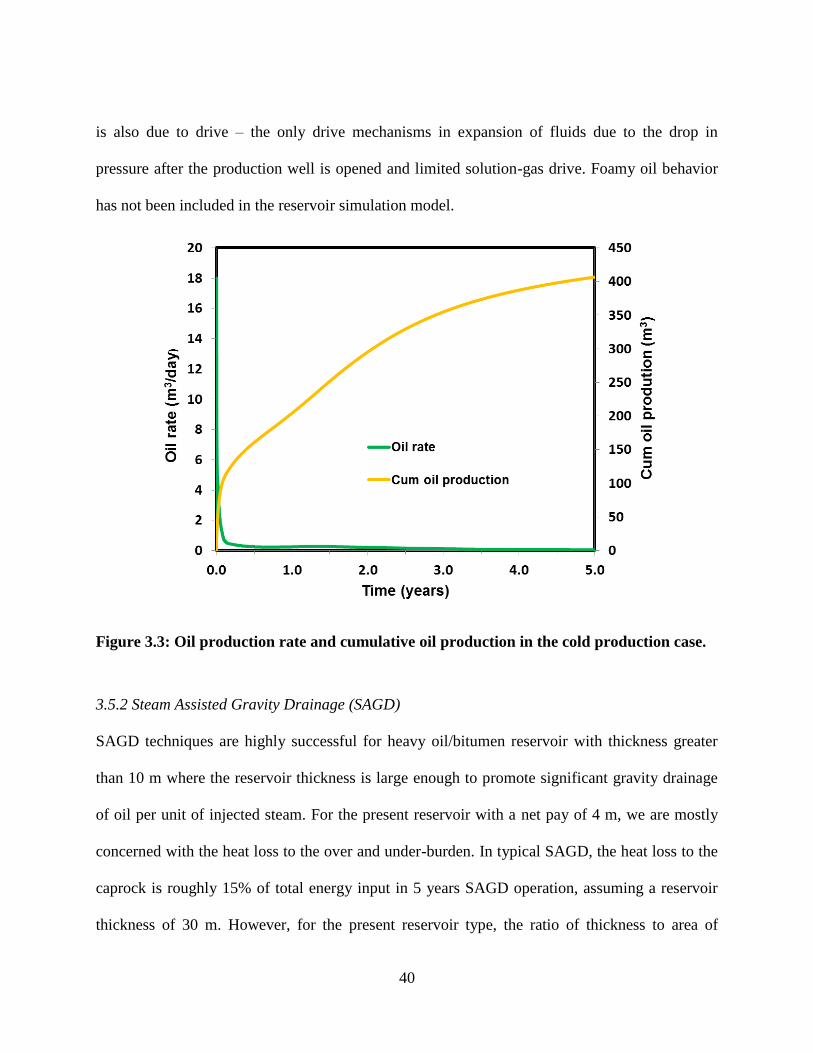
40

is also due to drive – the only drive mechanisms in expansion of fluids due to the drop in

pressure after the production well is opened and limited solution-gas drive. Foamy oil behavior

has not been included in the reservoir simulation model.

Figure 3.3: Oil production rate and cumulative oil production in the cold production case.

3.5.2 Steam Assisted Gravity Drainage (SAGD)

SAGD techniques are highly successful for heavy oil/bitumen reservoir with thickness greater

than 10 m where the reservoir thickness is large enough to promote significant gravity drainage

of oil per unit of injected steam. For the present reservoir with a net pay of 4 m, we are mostly

concerned with the heat loss to the over and under-burden. In typical SAGD, the heat loss to the

caprock is roughly 15% of total energy input in 5 years SAGD operation, assuming a reservoir

thickness of 30 m. However, for the present reservoir type, the ratio of thickness to area of

41

heated caprock is much lower. In the well placements considered here, this effect is compounded

because the injection well is 0.6 m below the caprock.

Figure 3.4a shows the temperature profile development which indicates the growth of steam

chamber. Differing from a typical SAGD chamber which grows from the lower part of the

reservoir, the steam chamber started to expand at the top due to the location of the steam injector.

As a result, the steam chamber formed an inverse triangle shape, as shown in Figure 3.4b. This

indicated a potentially large heat loss to the overburden as the process evolves.

(a)

(b)

Figure 3.4: Cross-section of (a) temperature distributions in the SAGD case after 3 months,

1 year, and 2 years later (ordered from top to bottom) and (b) phase distribution 1 year

42

after operation. The cross-sections are taken at a location 325 m from the heel of the

wellpair.

As shown in Figure 3.5, the oil production rate peaked at about 116 m3/day on the first day days

of steam injection. Thereafter, the oil rate dropped to about 25 m3/day after one year of

production with a cumulative oil production equal to 13,834 m3. Beyond the first year, the oil

rate decayed at a slower pace until after 4 years of production it reached below 10 m3/day. The

application of SAGD realized an oil recovery rate of 59.5% in 15 years. This is significantly

higher than cold production, however, the cumulative steam-to-oil ratio (cSOR) was equal to 7.5

m3 steam (steam expressed as cold water equivalent) per m

3 oil produced after one year. By the

end of 4 years, the cSOR exceeded 12.8 m3/m

3. A comparison between the performances of cold

production and SAGD can be found in Table 3.2.

Figure 3.5: Oil production rate in the SAGD case.

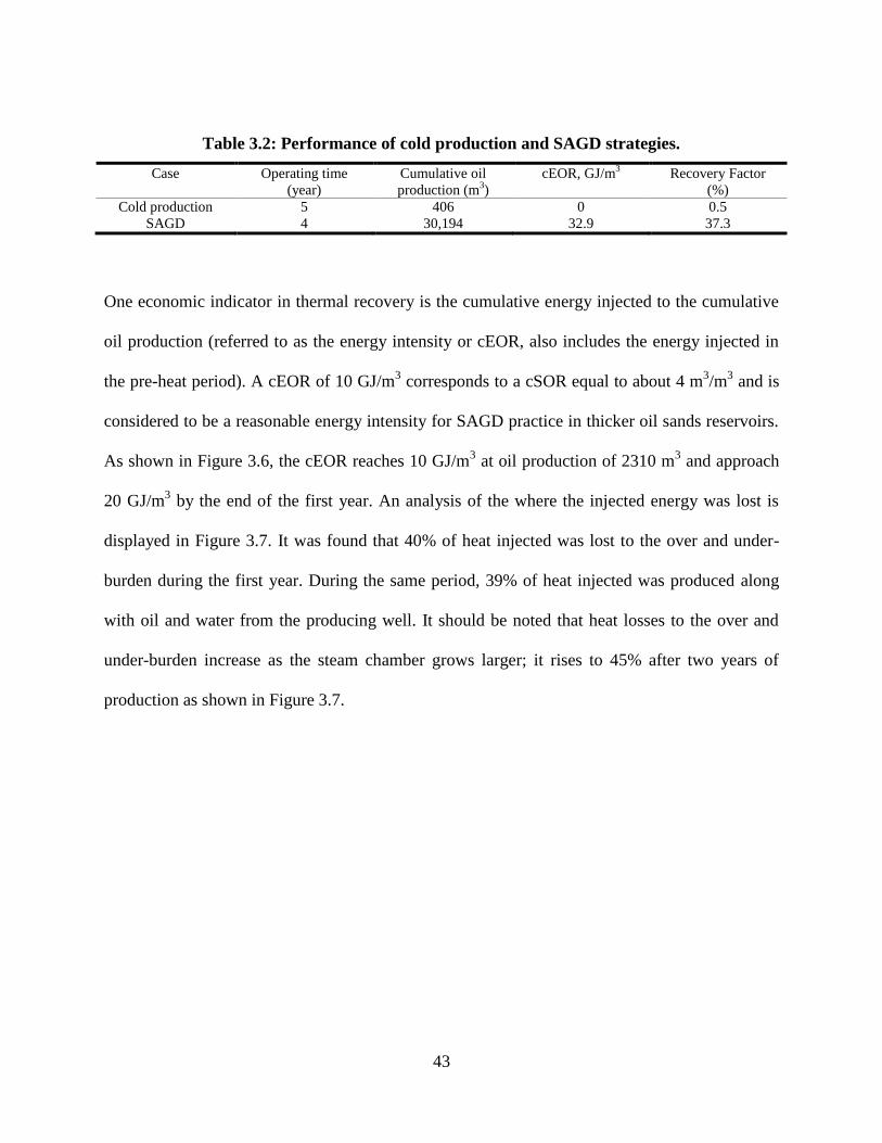
43

Table 3.2: Performance of cold production and SAGD strategies.

Case Operating time

(year)

Cumulative oil

production (m3)

cEOR, GJ/m3 Recovery Factor

(%)

Cold production 5 406 0 0.5

SAGD 4 30,194 32.9 37.3

One economic indicator in thermal recovery is the cumulative energy injected to the cumulative

oil production (referred to as the energy intensity or cEOR, also includes the energy injected in

the pre-heat period). A cEOR of 10 GJ/m3 corresponds to a cSOR equal to about 4 m

3/m

3 and is

considered to be a reasonable energy intensity for SAGD practice in thicker oil sands reservoirs.

As shown in Figure 3.6, the cEOR reaches 10 GJ/m3 at oil production of 2310 m

3 and approach

20 GJ/m3 by the end of the first year. An analysis of the where the injected energy was lost is

displayed in Figure 3.7. It was found that 40% of heat injected was lost to the over and under-

burden during the first year. During the same period, 39% of heat injected was produced along

with oil and water from the producing well. It should be noted that heat losses to the over and

under-burden increase as the steam chamber grows larger; it rises to 45% after two years of

production as shown in Figure 3.7.

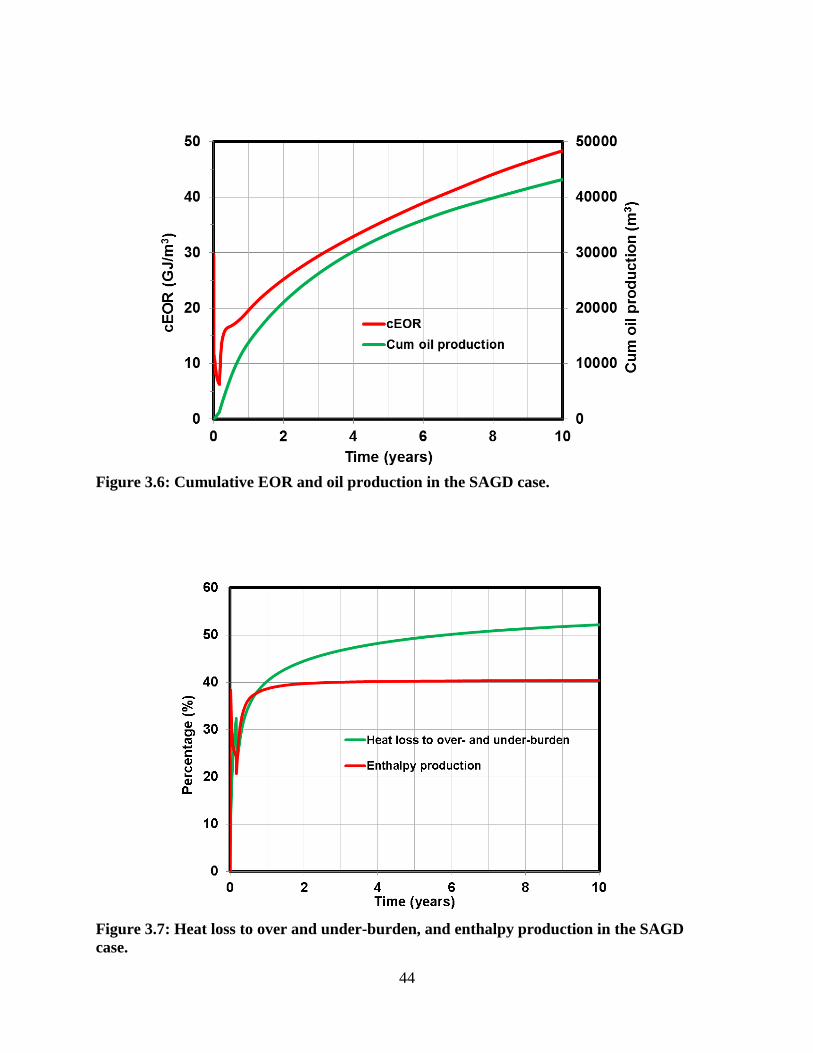
44

Figure 3.6: Cumulative EOR and oil production in the SAGD case.

Figure 3.7: Heat loss to over and under-burden, and enthalpy production in the SAGD

case.

45

The results demonstrate that heat utilization for SAGD in the present case is rather inefficient

compared to SAGD in thicker reservoirs. The poor performance of SAGD is due to large heat

losses to the over and underburden which in turn led to condensation of injected steam which led

to high temperature water production from the system. Since the hot water did not contact oil

rich zones, this led to heat transfer to oil at the edge of the chamber and low sweep efficiency.

3.5.3 Steam flooding

Steam flooding provides an additional drive mechanism to that of SAGD, that is, steam pressure

drive. In the cases considered here, it is assumed that the placement of injecting and producing

wells is periodic. To take advantage of this geometry, the injector and producer were put on the

side boundaries of the reservoir (these boundaries are symmetry boundaries). A water-cut limit is

set on the production well to be equal to 95% (by volume). Once this limit has been reached, the

injector is shut in and a blow-down strategy is employed with a lower oil rate cutoff of 2 m3/day

(at the production well), at which the operation is terminated.

Figure 3.8 shows the steam injection rates at different well separations. A general feature of the

results is that the steam injection rate decays initially for a period of time. It is suggested that the

initial decay resulted from the increasing reservoir pressure in the neighborhood of the injector

along with continuing steam injection. With greater time, the water saturation in the reservoir

increases which gives rise to increase of fluid mobility and thereafter a higher steam injectivity.

46

Figure 3.8: Steam injection rates in steam-flooding cases at different well separation.

(a)

(b)

(c)

Figure 3.9: Oil saturation distribution in a steamflooding model with a well separation

equal to 40 m: (a) 6 months of production (top), (b) 2 years of production (middle), and (c)

2.58 years later when injector is shut in and a blowdown strategy is implemented. Cross-

section taken 325 m down length of the wells.

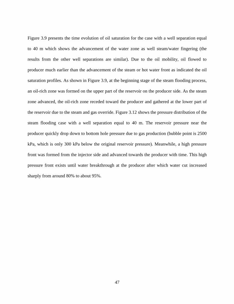
47

Figure 3.9 presents the time evolution of oil saturation for the case with a well separation equal

to 40 m which shows the advancement of the water zone as well steam/water fingering (the

results from the other well separations are similar). Due to the oil mobility, oil flowed to

producer much earlier than the advancement of the steam or hot water front as indicated the oil

saturation profiles. As shown in Figure 3.9, at the beginning stage of the steam flooding process,

an oil-rich zone was formed on the upper part of the reservoir on the producer side. As the steam

zone advanced, the oil-rich zone receded toward the producer and gathered at the lower part of

the reservoir due to the steam and gas override. Figure 3.12 shows the pressure distribution of the

steam flooding case with a well separation equal to 40 m. The reservoir pressure near the

producer quickly drop down to bottom hole pressure due to gas production (bubble point is 2500

kPa, which is only 300 kPa below the original reservoir pressure). Meanwhile, a high pressure

front was formed from the injector side and advanced towards the producer with time. This high

pressure front exists until water breakthrough at the producer after which water cut increased

sharply from around 80% to about 95%.

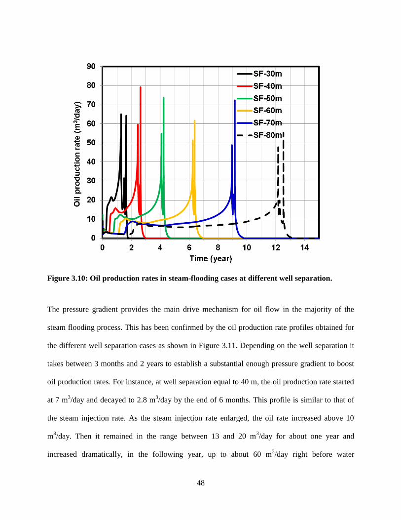
48

Figure 3.10: Oil production rates in steam-flooding cases at different well separation.

The pressure gradient provides the main drive mechanism for oil flow in the majority of the

steam flooding process. This has been confirmed by the oil production rate profiles obtained for

the different well separation cases as shown in Figure 3.11. Depending on the well separation it

takes between 3 months and 2 years to establish a substantial enough pressure gradient to boost

oil production rates. For instance, at well separation equal to 40 m, the oil production rate started

at 7 m3/day and decayed to 2.8 m

3/day by the end of 6 months. This profile is similar to that of

the steam injection rate. As the steam injection rate enlarged, the oil rate increased above 10

m3/day. Then it remained in the range between 13 and 20 m

3/day for about one year and

increased dramatically, in the following year, up to about 60 m3/day right before water

49

breakthrough. After injection was stopped, the oil rate dropped sharply down to 12 m3/day,

which was followed by a narrow peak during the three months long blowdown process. Similar

trends were found for the other well separation cases. In general, the larger the well separation,

the lower the oil production rate over a longer production period. In the 80 m well separation

case, it took more than 12 years for the water front to break through to the producer.

(a)

(b)

Figure 3.11: Cross-sections of (a) temperature distribution in steamflooding case with well

separation equal to 40 m, respectively, after 6 months, 2 years, and 2.58 years later when

the injector is shut in and a blowdown process is used (ordered from top to bottom) and (b)

phase distribution at 2.58 years (bottom). Cross-section taken 325 m down length of the

wells.

50

Figure 3.11 depicts the time evolution of the temperature distribution for the well separation case

equal to 40 m. The temperature distributions reveal that there is a hot water zone in front of the

steam zone. The steam zone itself, however, is not as well developed as in the SAGD case (see

Figure 3.11b). Even at the end of steam injection (due to water breakthrough), the steam zone did

not reach the middle point of the reservoir. In comparison, the pressure front advanced much fast

than the steam front as suggested by Figure 3.12. After the pressure front reached the producer,

the watercut increased quickly and eventually broke through to the producer after which the

reservoir pressure dropped sharply. The loss of reservoir pressure led to a drop in oil rate. The

three-month blowdown process was found to be able to recover an additional 2.5–5% of the

original oil in place depending on the well separation.

(a)

(b)

Figure 3.12: Pressure (in kPa) distribution in the steam flooding case with well separation

equal to 40 m: (a) 6 months after operation and (b) 2 years after operation. Cross-section

taken 325 m down length of the wells.

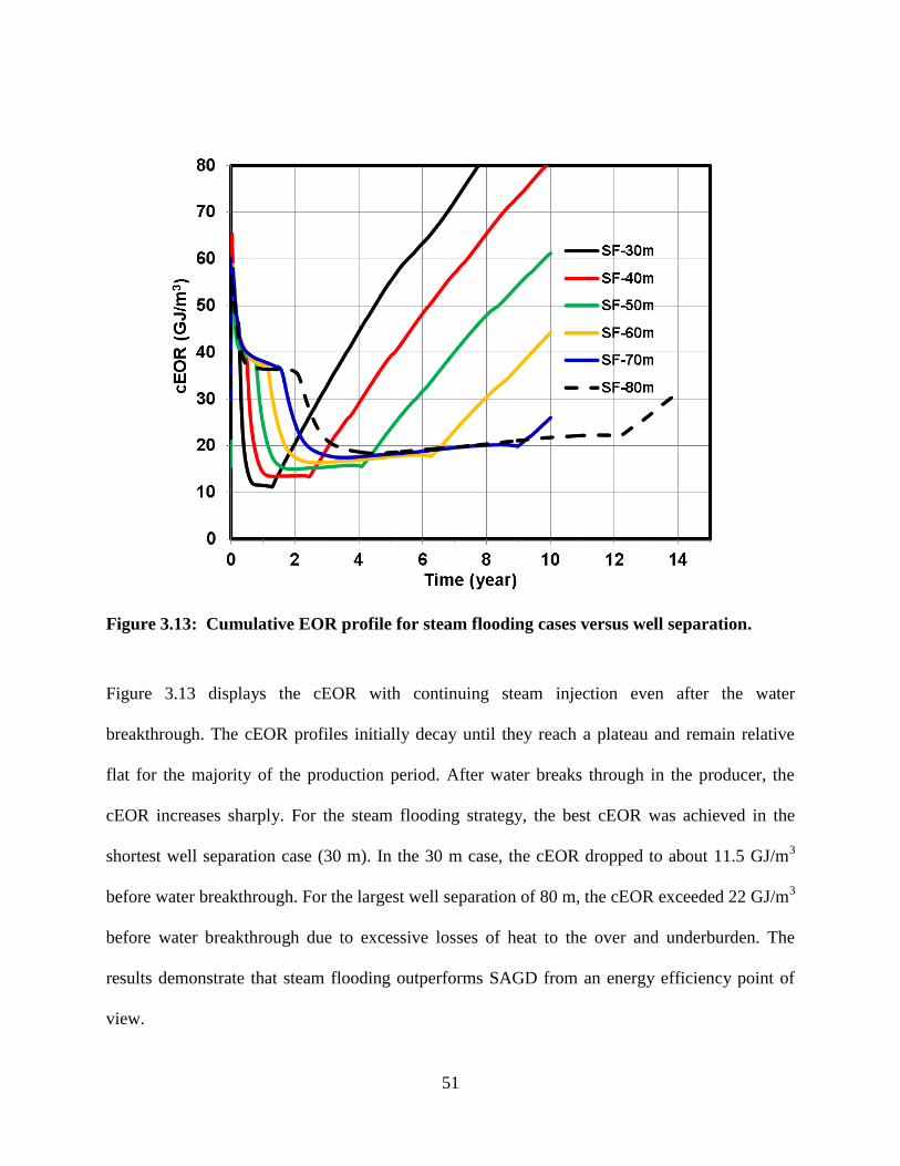
51

Figure 3.13: Cumulative EOR profile for steam flooding cases versus well separation.

Figure 3.13 displays the cEOR with continuing steam injection even after the water

breakthrough. The cEOR profiles initially decay until they reach a plateau and remain relative

flat for the majority of the production period. After water breaks through in the producer, the

cEOR increases sharply. For the steam flooding strategy, the best cEOR was achieved in the

shortest well separation case (30 m). In the 30 m case, the cEOR dropped to about 11.5 GJ/m3

before water breakthrough. For the largest well separation of 80 m, the cEOR exceeded 22 GJ/m3

before water breakthrough due to excessive losses of heat to the over and underburden. The

results demonstrate that steam flooding outperforms SAGD from an energy efficiency point of

view.

52

Table 3.3 summaries the performance of steamflooding for the different well separations. The

oil recovery factors are quite similar, ranging from 38 to 42%. At larger well distances,

however, cEORs become larger with a longer operating time.

Table 3.3: Performance of steam flooding at different well separations.

Well Separation

(m)

Operating time

(year)

Cumulative oil

production (m3)


(%)

30 1.72 12,601 13.7 41.9

40 2.82 15,224 13.6 37.9

50 4.48 19,275 15.2 38.4

60 6.68 23,721 17.2 39.4

70 9.47 28,704 18.9 40.9

80 12.80 33,353 20.9 41.6

3.5.4 Hot water flooding

As with SAGD, steam flooding suffers from excessive heat losses to the overburden. Steam

contains not only sensible heat of liquid water but a greater fraction of its energy is in the form of

latent heat. Considerable savings with respect to injected energy can be realized if hot water

alone is injected into the reservoir. Fig. 14 shows the time evolution of oil saturation in reservoir

with a well separation equal to 40 m. We found that it takes a longer time for water to break

through to the producer in the hot water flooding strategy. The oil saturation distribution is

different from that of the steam flooding cases: in the steam flooding cases, the highest oil

53

saturations are in the lower parts of the reservoir due to steam override whereas in the water

flooding cases, the highest oil saturations are found in the upper parts of the reservoir.

(a)

(b)

(c)

Figure 3.14: Oil saturations at different times in the water-flooding with well separation

equal to 40 m: (a) 6 months later, (b) 2 years later, and (c) 2.8 years after which injector is

shut in and blowdown strategy is employed. Cross-section taken 325 m down length of the

wells.

The oil production rate profiles achieved by using hot water flooding are found to be quite

similar to that by using steam flooding strategy, as shown in Figure 3.15. However, the water

front advanced at a slightly slower pace in the hot water flooding cases. The oil production curve

exhibits a lower but broader peak before water break through in the water flooding cases. In the

40 m hot water flooding case, the production time is two months longer than the steam flooding

case. In the 80 m reservoir, the operating time in water flooding is 6 months longer than that in

steam flooding. The faster advancement of the water front in steam flooding is due to the greater

54

energy associated with steam – in the hot water flooding cases, the water loses sensible heat

which leads to lower temperature whereas in the steam cases, the steam remains at the same

temperature until all of the steam is condensed.

Figure 3.15: Oil production rates of hot water flooding cases versus well separation.

55

Figure 3.16: Cumulative EOR profiles of hot water flooding cases versus well separation.

(a)

(b)

Figure 3.17: Temperature (in °C) distributions on the day when injector is shut in 40 m

well separation case: (a) steam flooding and (b) hot water flooding. Cross-section taken 325

m down length of the wells.

56

As shown in Figure 3.16, a much lower cEOR results in the hot water flooding cases compared

to the steam flooding cases. For example, at a well separation of 40 m, the cEOR bottoms at 8.5

GJ/mol at the end of the first two years of production and achieve an overall cEOR of 9.1 GJ/m3

after water breakthrough. These cEOR’s are comparable to current economic SAGD operations.

Even at a well separation of 80 m, the hot water flood cEOR realized is comparable to that in the

steam flooding case with a well separation equal to 30 m. We suggest that the lower energy

injected (since no latent heat in the hot water flooding cases) and lower temperature distributions

encountered as a result in the reservoir in the hot water flooding cases led to lower heat losses to

the over and underburden; see Figure 3.17: the reservoir temperature of the hot water flooding

case, on average, is lower than that in the steam flooding case.

(a)

(b)

Figure 3.18: Oil viscosity (in cP) distributions after 6 months of production in case with 40

m well separation: (a) steam flooding case and (b) hot water flooding case. Cross-section

taken 325 m down length of the wells.

Figure 3.18 shows the oil viscosity profiles the steam flooding and hot water flooding cases after

6 months of operation. The oil viscosity reduction is actually larger in the hot water injection

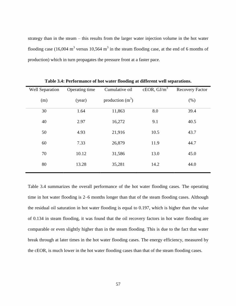
57

strategy than in the steam – this results from the larger water injection volume in the hot water

flooding case (16,004 m3 versus 10,564 m

3 in the steam flooding case, at the end of 6 months of

production) which in turn propagates the pressure front at a faster pace.

Table 3.4: Performance of hot water flooding at different well separations.

Well Separation

(m)

Operating time

(year)

Cumulative oil

production (m3)


(%)

30 1.64 11,863 8.0 39.4

40 2.97 16,272 9.1 40.5

50 4.93 21,916 10.5 43.7

60 7.33 26,879 11.9 44.7

70 10.12 31,586 13.0 45.0

80 13.28 35,281 14.2 44.0

Table 3.4 summarizes the overall performance of the hot water flooding cases. The operating

time in hot water flooding is 2–6 months longer than that of the steam flooding cases. Although

the residual oil saturation in hot water flooding is equal to 0.197, which is higher than the value

of 0.134 in steam flooding, it was found that the oil recovery factors in hot water flooding are

comparable or even slightly higher than in the steam flooding. This is due to the fact that water

break through at later times in the hot water flooding cases. The energy efficiency, measured by

the cEOR, is much lower in the hot water flooding cases than that of the steam flooding cases.

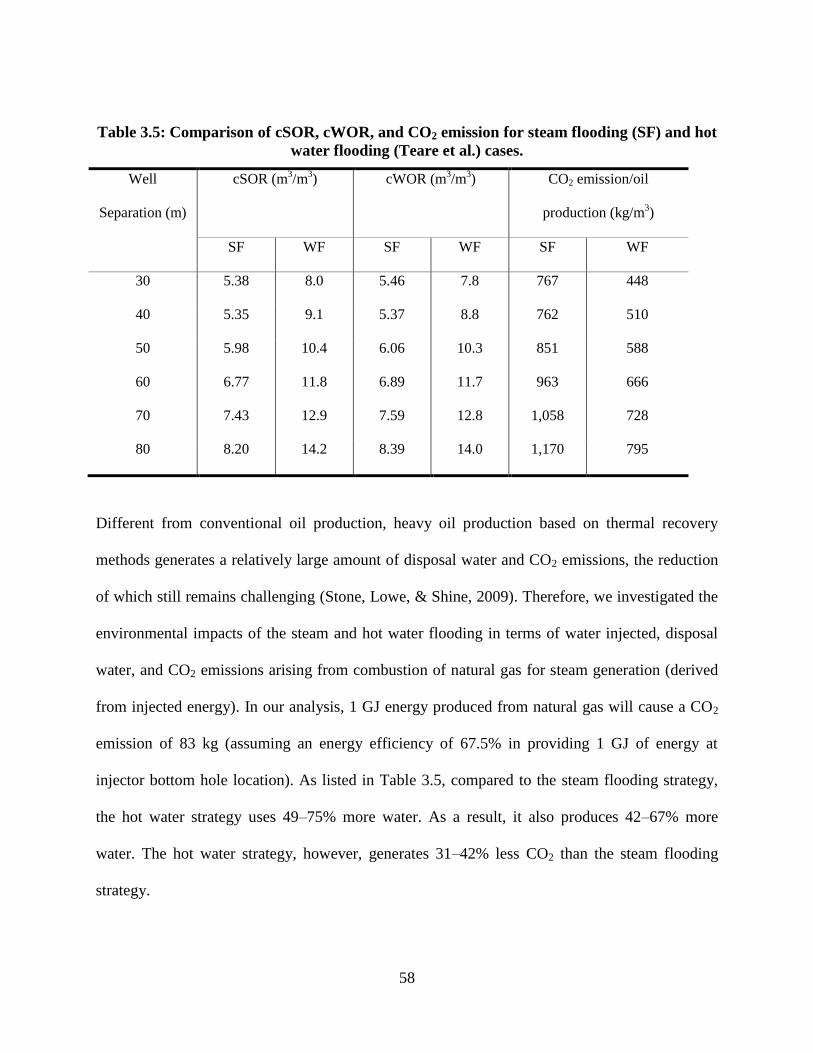
58

Table 3.5: Comparison of cSOR, cWOR, and CO2 emission for steam flooding (SF) and hot

water flooding (Teare et al.) cases.

Well

Separation (m)

cSOR (m3/m

3) cWOR (m

3/m

3) CO2 emission/oil

production (kg/m3)

SF WF SF WF SF WF

30 5.38 8.0 5.46 7.8 767 448

40 5.35 9.1 5.37 8.8 762 510

50 5.98 10.4 6.06 10.3 851 588

60 6.77 11.8 6.89 11.7 963 666

70 7.43 12.9 7.59 12.8 1,058 728

80 8.20 14.2 8.39 14.0 1,170 795

Different from conventional oil production, heavy oil production based on thermal recovery

methods generates a relatively large amount of disposal water and CO2 emissions, the reduction

of which still remains challenging (Stone, Lowe, & Shine, 2009). Therefore, we investigated the

environmental impacts of the steam and hot water flooding in terms of water injected, disposal

water, and CO2 emissions arising from combustion of natural gas for steam generation (derived

from injected energy). In our analysis, 1 GJ energy produced from natural gas will cause a CO2

emission of 83 kg (assuming an energy efficiency of 67.5% in providing 1 GJ of energy at

injector bottom hole location). As listed in Table 3.5, compared to the steam flooding strategy,

the hot water strategy uses 49–75% more water. As a result, it also produces 42–67% more

water. The hot water strategy, however, generates 31–42% less CO2 than the steam flooding

strategy.

59

3.5.3 Alternating Steam and Hot Water Flooding

As done in Cold Lake, CSS is used as an individual well steam-fracturing recovery process in

early cycles which then shifts to a cyclic steam flooding operation in later cycles as interwell

communication starts to dominate the process – this practice is often referred to as the megarow

CSS strategy. Being a cyclic process, all wells are used as injectors and as producers over

different time periods. Here, this strategy has been applied without steam fracturing: one well is

first used as injector and the other one as producer. After a certain period of time, the injector is

turned into a producer and the producer is switched to an injector.

Figure 3.19: Cumulative EOR and oil production profiles in the alternating water-flooding

cases.

60

The main purpose of this strategy is to increase the reservoir temperature on its both sides and

increase the oil mobility more efficiently. A test study is carried out for a reservoir with a well

distance of 40 m with two different cycle periods of 1 year and 6 months.

Figure 3.19 displays the cEOR and cumulative oil production of the cases in comparison with the

hot water flooding 40 m case discussed above. It can be seen that the cEOR of these two

alternating water flooding cases is higher than the uni-directional water flooding while achieving

a lower oil production performance. Similar results were also found in alternating steam flooding

cases. Although this strategy was suggested by a previous study (Edgar et al., 2008) that it could

achieve performances similar to SAGD for thicker heavy oil reservoirs, it is not successful in the

present study.

There are two reasons behind this unsuccessful strategy. First, the injected energy is not efficient

in heating the reservoir due to the heat loss to the over- and underburden, though it does provide

driving energy to fluid flow in the reservoir. Second, due to the oil mobility at reservoir

temperature the injected steam/hot water drive oil away from injector and created a water-rich

zone in the neighborhood of the injector. After the steam/hot water injectors are switched to

producers, they produce mainly hot water before oil production. Therefore the alternating

steam/hot water flooding performs poorly compared to the steam and hot water flooding cases.

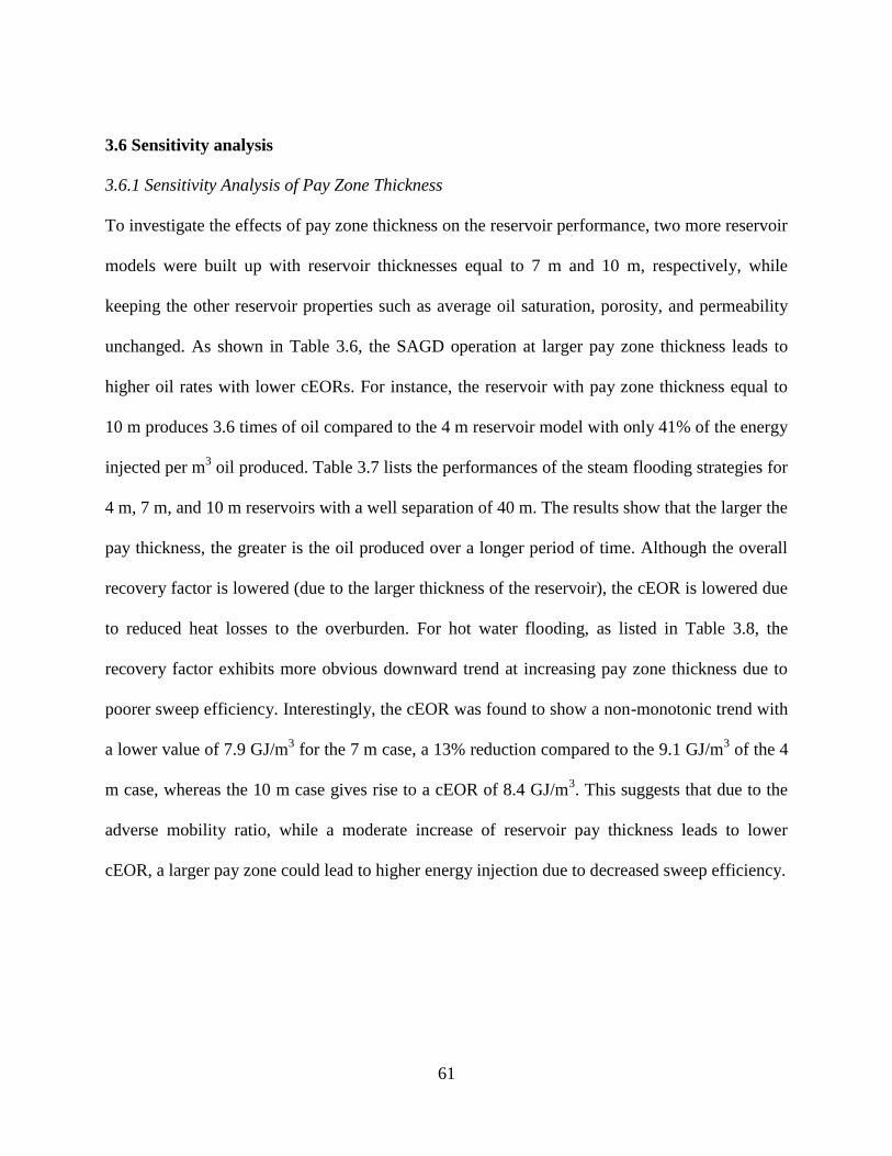
61

3.6 Sensitivity analysis

3.6.1 Sensitivity Analysis of Pay Zone Thickness

To investigate the effects of pay zone thickness on the reservoir performance, two more reservoir

models were built up with reservoir thicknesses equal to 7 m and 10 m, respectively, while

keeping the other reservoir properties such as average oil saturation, porosity, and permeability

unchanged. As shown in Table 3.6, the SAGD operation at larger pay zone thickness leads to

higher oil rates with lower cEORs. For instance, the reservoir with pay zone thickness equal to

10 m produces 3.6 times of oil compared to the 4 m reservoir model with only 41% of the energy

injected per m3 oil produced. Table 3.7 lists the performances of the steam flooding strategies for

4 m, 7 m, and 10 m reservoirs with a well separation of 40 m. The results show that the larger the

pay thickness, the greater is the oil produced over a longer period of time. Although the overall

recovery factor is lowered (due to the larger thickness of the reservoir), the cEOR is lowered due

to reduced heat losses to the overburden. For hot water flooding, as listed in Table 3.8, the

recovery factor exhibits more obvious downward trend at increasing pay zone thickness due to

poorer sweep efficiency. Interestingly, the cEOR was found to show a non-monotonic trend with

a lower value of 7.9 GJ/m3 for the 7 m case, a 13% reduction compared to the 9.1 GJ/m

3 of the 4

m case, whereas the 10 m case gives rise to a cEOR of 8.4 GJ/m3. This suggests that due to the

adverse mobility ratio, while a moderate increase of reservoir pay thickness leads to lower

cEOR, a larger pay zone could lead to higher energy injection due to decreased sweep efficiency.

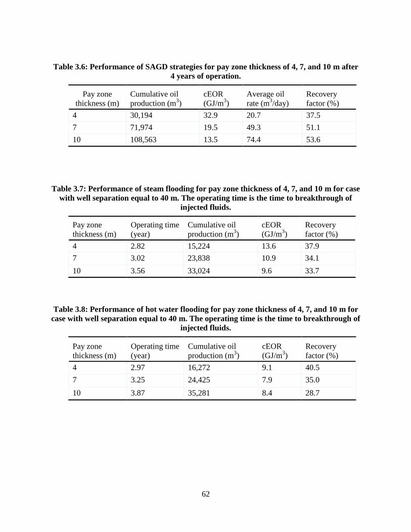
62

Table 3.6: Performance of SAGD strategies for pay zone thickness of 4, 7, and 10 m after

4 years of operation.

Pay zone

thickness (m)

Cumulative oil

production (m3)

cEOR

(GJ/m3)

Average oil

rate (m3/day)

Recovery

factor (%)

4 30,194 32.9 20.7 37.5

7 71,974 19.5 49.3 51.1

10 108,563 13.5 74.4 53.6

Table 3.7: Performance of steam flooding for pay zone thickness of 4, 7, and 10 m for case

with well separation equal to 40 m. The operating time is the time to breakthrough of

injected fluids.

Pay zone

thickness (m)

Operating time

(year)

Cumulative oil

production (m3)

cEOR

(GJ/m3)

Recovery

factor (%)

4 2.82 15,224 13.6 37.9

7 3.02 23,838 10.9 34.1

10 3.56 33,024 9.6 33.7

Table 3.8: Performance of hot water flooding for pay zone thickness of 4, 7, and 10 m for

case with well separation equal to 40 m. The operating time is the time to breakthrough of

injected fluids.

Pay zone

thickness (m)

Operating time

(year)

Cumulative oil

production (m3)

cEOR

(GJ/m3)

Recovery

factor (%)

4 2.97 16,272 9.1 40.5

7 3.25 24,425 7.9 35.0

10 3.87 35,281 8.4 28.7

63

3.6.2 Sensitivity Analysis of Steam Quality on the Performance of Steam Flooding

To understand the role of steam quality on the performance of steam flooding, additional

simulations were done for the case with well separation equal to 40 m. The results are listed in

Table 3.9. The results show that the steam quality impacts oil production. At steam qualities

equal to 0.3 and 0.6, the recovery factor is raised by 2.3% and 2.6%, respectively, compared to

the hot water case. However, at steam quality equal to 0.9, the recovery factor drops below that

of the hot water case. We suggest that using a combined mixture of hot water and steam leads to

a more uniform water front in the vertical direction than that achieved in the hot water case (front

moves faster at the bottom of the reservoir) and that achieved in the steam case (front moves

faster at the top of the reservoir). This means more reservoir volume will be swept by the mixture

of hot water and steam injection. However, increased steam quality significantly increases the

energy injection per m3 oil production. An increase of steam quality from 0.0 to 0.3 gives rise to

an additional 5% volume of oil produced but at the expense of 21% extra energy injected into the

reservoir.

Table 3.9:Performance of steam flooding using steam quality of 0.0 (hot water), 0.3, 0.6 and

0.9 for pay zone thickness of 4 m for case with well separation equal to 40 m. The operating

time is the time to breakthrough of injected fluids.

Steam

quality

Operating time

(year)

Cumulative oil

production (m3)

cEOR

(GJ/m3)

Recovery factor

(%)

0.0 2.97 16,272 9.1 40.5

0.3 3.02 17,163 11.0 42.8

0.6 3.02 17,318 12.6 43.1

0.9 2.82 15,224 13.6 37.9

64

3.7 Conclusions

A study to determine how thermal processes perform in thin (<5 m) heavy oil reservoirs was

conducted by using reservoir simulation. The average porosity, horizontal permeability, and oil

saturation of the reservoir was equal to 0.32, 3,650 mD, and 0.65, respectively. The live oil

viscosity at original reservoir conditions was equal to 8917 cP and original solution gas-to-oil

ratio was equal to 6.17 m3/m

3. From the results of the study, the following conclusions can be

made:

1. Cold production (without sand) is not applicable to thin heavy oil reservoir under study.

Depletion of reservoir pressure and high water saturation make the oil production rate low and

recovery factor less than 1%.

2. SAGD achieved a recovery factor of 37% with a cumulative steam-to-oil ratio (cSOR) equal

to 12.8 m3/m

3 at the end of 4 years of operation. The cumulative energy injected to oil ratio

(cEOR) at the end of the process was equal to 32.9 GJ/m3. The major reason for the high cSOR

(and cEOR) is heat loss to over and underburden and hot water production from the system.

3. Steam-flooding strategy achieved much better performance compared to SAGD operation in

terms of cEOR. However, it is still most likely economically expensive because of its higher

cEOR, ranging from 13.6 to 20.9 GJ/m3 compared to that of the SAGD case. Similar to the

SAGD case, this is due to the excess heat loss to caprock.

65

4. Alternating injection/production well steam and hot water flooding strategies were not found

to be effective.

5. The sensitivity analysis on reservoir thickness suggests that both SAGD and steam flooding

operation are becoming more favorable for a larger pay zone thickness and leads to better

performance. The sensitivity analysis on steam quality indicates that more oil is produced with

higher steam quality, however, it is more energy-efficient to use a lower steam quality to reduce

the cEOR.

6. Hot water flooding is more effective compared with steam flooding with respect to cEOR. The

oil rate resulted from the pressure gradient rather than oil viscosity reduction due to the injected

heat. The use of hot water led to a lower average reservoir temperature and therefore reduced

heat loss to the over and underburden. The achieved cEOR ranged from 8 to 14 GJ/m3 depending

on the well separation with additional environmental benefits in terms of CO2 emissions. Given

that SAGD is economic at cEORs up to about 13 GJ/m3 (corresponds to cSOR equal to about 5

m3/m

3), hot water appears to be worth examining more in laboratory experiments or a field trial.

However, since the range of hot water flooding cEOR and water use are still relatively high,

thermal-solvent methods should be examined (L. Dong, 2012).

3.8 References

Adams, D. M. (1982). Experiences With Waterflooding Lloydminster Heavy-Oil Reservoirs.


Asghari, K., & Nakutnyym, P. (2008). Experimental Results of Polymer Flooding of Heavy Oil

Reservoirs. Paper presented at the The Canadian International Petroleum Conference/SPE

66

Gas Technology Symposium 2008 Joint Conference (the Petroleum Society’s 59th

Annual Technical Meeting), Calgary, Alberta, Canada.

Canadian Natural Resources Ltd. (2011). Canadian Natural Resources Ltd, 2010 Annual Report

Retrieved from http://www.cnrl.com/upload/media_element/385/01/cn_2010ar.pdf

Dong, L. (2012). Effect of vapor-liquid phase behavior of steam-light hydrocarbon systems on

steam assisted gravity drainage process for bitumen recovery Fuel, 95, 159-168.

Dong, M., Ma, S., & Liu, Q. (2009). Enhanced heavy oil recovery through interfacial instability:

a study of chemical flooding for Brintnell heavy oil. Fuel, 88, 1049-1056.

Edgar, A., Fernandez, R., & Bashbush, J. L. (2008). Horizontal Alternate Steam Drive Process

for the Orinoco Heavy Oil Belt in Eastern Venezuela. Paper presented at the International

Thermal Operations and Heavy Oil Symposium, Calgary, Alberta, Canada.

Gao, C.-H. (2011). Advances of Polymer Flood in Heavy Oil Recovery. Paper presented at the

The 2011 SPE Heavy Oil Conference and Exhibition, Kuwait City, Kuwait.

Gates, I. D. (2010). Solvent-aided Steam-Assisted Gravity Drainage in thin oil sand reservoirs.

Journal of Petroleum Science and Engineering, 74, 138-146.

Jamaloei, B. Y., Kharrat, R., & Asghari, K. (2012). The influence of salinity on the viscous

instability in viscous-modified low-interfacial tension flow during surfactant-polymer

flooding in heavy oil reservoir. Fuel, 97, 174-185.

CMG Ltd., (2012). STARSTM

User’s Guide.




Pan, Y., Chen, Z., Sun, J., Bao, X., Xiao, L., & Wang, R. (2010). Research progress of

modelling on cold heavy oil production with sand. . Paper presented at the The SPE

Western Regional Meeting, Anaheim, Califonia, USA.

Reddy, J. N. (2005). An Introduction to the Finite Element Method (3rd Ed.): McGraw-Hill.



700-714.



Stone, E. J., Lowe, J. A., & Shine, K. P. (2009). Thee impact of carbon capture and storage on

climate. Energy Environ. Sci., 2, 81-91.

Tavallali, M., Maini, B., & Harding, T. (2012). Assessment of SAGD Well Configuration

Optimization in Lloyminster Heavy Oil Reserve. Paper presented at the the SPE/EAGE

European Unconventional Resources Conference and Exhibition, Vienna, Austria.

Teare, M., Burrowes, A., Baturin-Pollock, C., Rokosh, D., Evans, C., Gigantelli, P., . . .

Crowfoot, C. (2012). Alberta’s Energy Reserves 2011 and Supply/Demand Outlook

2012–2021.

http://www.cnrl.com/upload/media_element/385/01/cn_2010ar.pdf

67

CHAPTER FOUR: ON HOT WATER FLOODING STRATEGIES FOR THIN HEAVY

OIL RESERVOIRS


citation is as follows: Zhao, D. and Gates, I.D. On Hot Water Flooding Strategies for Thin

Heavy Oil Reservoirs. Fuel, 153:559-568, 2015.

4.1 Abstract

Cold production methods for heavy oil resources in Western Canada yield recovery factors

averaging about 10% and as yet, there are no commercially successful technologies to produce

oil from these reservoirs with recovery factor greater than 20%. This means that the majority of

oil remains in the reservoir. The objective of this study is to determine technically and

economically feasible recovery processes for thin heavy oil reservoirs by using a simulated

annealing algorithm. The results reveal that high injection pressure is critical to a successful hot

water flooding strategy. Also, they show from a thermal efficiency point of view that it is most

efficient to adopt an injection temperature profile where the injection temperature starts high

earlier in the process and ends at lower water temperature. The lower temperature injection at

later stages of the recovery process partially recovers the heat stored in the reservoir matrix and

therefore increases the overall heat utilization efficiency. A sensitivity analysis shows that the

permeability distribution affects the performance of the hot water flooding process most

significantly. The existence of a higher permeability zone in the lower part of the reservoir leads

to earlier oil production and water breakthrough. High permeability was found to lead to more oil

and water production in the early stage of operation and achieved the best economic

performance. The low permeability case exhibited relatively low oil production volume.

68

Although it has the lowest cumulative injected energy to oil produced ratio, poor oil production

renders the operation process uneconomic. Given the volume of currently inaccessible thin heavy

oil resources, the optimized strategies developed here provide important guidelines to convert

these resources to producible reserves.

4.2 Introduction

The majority of heavy oil resources in the Western Canada Sedimentary Basin are found in thin

reservoirs with thickness less than 6 m (Adams, 1982). Due to heat losses to the overburden or

understrata or both, current commercial steam-based techniques such as Steam-Assisted Gravity

Drainage (SAGD) and Cyclic Steam Stimulation (CSS) are not economically feasible in thin

heavy oil reservoirs (<6 m).

In these processes, in thin reservoirs, the amount of steam invested in the reservoir versus the oil

revenues renders the processes uneconomic. In cold production (CP) processes, the only energy

input is that of the pump to move the produced fluids from the reservoir to the surface; thus their

energy investment is relatively small. However, the average recovery factors of cold production

processes are low being equal to about 10% (Adams, 1982). By encouraging sand production

along with oil recovery, the Cold Heavy Oil Production with Sand (CHOPS) technique can

recover as much as 15% of the OOIP (Pan et al., 2010). In CHOPS operations, sand production

creates an extensive connected wormhole network in the reservoir with zones adjacent to the

network depleted of reservoir pressure (Istchenko and Gates, 2014).

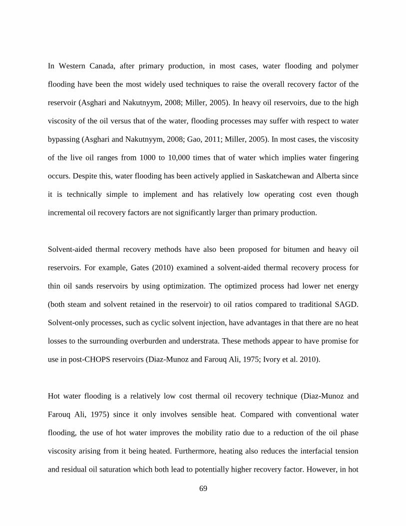
69

In Western Canada, after primary production, in most cases, water flooding and polymer

flooding have been the most widely used techniques to raise the overall recovery factor of the

reservoir (Asghari and Nakutnyym, 2008; Miller, 2005). In heavy oil reservoirs, due to the high

viscosity of the oil versus that of the water, flooding processes may suffer with respect to water

bypassing (Asghari and Nakutnyym, 2008; Gao, 2011; Miller, 2005). In most cases, the viscosity

of the live oil ranges from 1000 to 10,000 times that of water which implies water fingering

occurs. Despite this, water flooding has been actively applied in Saskatchewan and Alberta since

it is technically simple to implement and has relatively low operating cost even though

incremental oil recovery factors are not significantly larger than primary production.

Solvent-aided thermal recovery methods have also been proposed for bitumen and heavy oil

reservoirs. For example, Gates (2010) examined a solvent-aided thermal recovery process for

thin oil sands reservoirs by using optimization. The optimized process had lower net energy

(both steam and solvent retained in the reservoir) to oil ratios compared to traditional SAGD.

Solvent-only processes, such as cyclic solvent injection, have advantages in that there are no heat

losses to the surrounding overburden and understrata. These methods appear to have promise for

use in post-CHOPS reservoirs (Diaz-Munoz and Farouq Ali, 1975; Ivory et al. 2010).

Hot water flooding is a relatively low cost thermal oil recovery technique (Diaz-Munoz and

Farouq Ali, 1975) since it only involves sensible heat. Compared with conventional water

flooding, the use of hot water improves the mobility ratio due to a reduction of the oil phase

viscosity arising from it being heated. Furthermore, heating also reduces the interfacial tension

and residual oil saturation which both lead to potentially higher recovery factor. However, in hot

70

water flooding, the heated water for injection delivers less heat to the reservoir compared to that

with steam due to absence of latent heat and therefore it is less effective in reducing oil viscosity.

On the other hand, for thin heavy oil reservoirs, hot water flooding has advantages over steam

flooding. First, it provides larger displacement drive than steam flooding since water viscosity is

much larger than that of steam (Diaz-Munoz and Farouq Ali, 1975; Gates, 2011; Martin et al.,

1967). Second, it permits the use of much higher injection pressure than steam flooding at a

given temperature. Furthermore, higher-pressure injection enables greater temperatures while

remaining in the hot water state. Third, due to smaller reservoir temperature, heat losses to the

overburden and understrata will be substantially smaller than that encountered in steam flooding.

However, less heat losses to the overburden and understrata will mean less heat delivery to the

heavy oil interval.

Martin et al. describe the results of hot water injection into a 5–7 m thick sandstone reservoir

containing oil with viscosity equal to 600 cP (Martin et al., 1967). They found that water

injectivity and oil rates were significantly enhanced over that of cold water flooding. However,

although they did not have detailed thermocouple observation wells, they concluded that 60

percent of the injected heat was lost to the overburden and understrata. Thus, there is a need to

design hot water recovery processes for thin reservoirs that manage heat delivery and recovery to

and within the reservoir.

In the study documented here, hot water-flooding strategies are optimized by using simulated

annealing, a stochastic optimization algorithm. We aimed to understand the effects of injection

71

pressure, water temperature, as well as different reservoir conditions on the recovery process

performance.

4.3 Models and Methods

4.3.1 Reservoir Simulation Models

The reservoir evaluated here has properties typical of that of a typical thin heavy oil reservoir in

the Lloydminster area of Alberta, Canada described in a previous study (Zhao, Wang, & Gates,

2014). The base case reservoir model is two-dimensional with two horizontal wells spaced 50 m

apart. The thickness of the heavy oil interval is equal to 4 m thick. The models were discretized

into a regular Cartesian grid, displayed in Figure 4.1, with dimensions 1 m in the cross-well

direction, 1000 m in the down-well direction (into the page) and 0.4 m in the vertical direction.

The length of the perforated sections of the horizontal wells in all models is equal to 1000 m. A

commercial thermal reservoir simulator (CMG STARS™) was used. The commercial thermal

reservoir simulator uses the finite volume approach. At the top and bottom boundaries, heat

losses were permitted and were approximated by using Vinsome and Westerveld’s (1980) heat

loss model. At the side boundaries of the model, no flow and no heat transfer boundary

conditions were applied.

The reservoir simulation model and fluid properties are listed in Table 4.1. The relative

permeability curves, listed in Table 4.1, are independent of temperature. The spatial distributions

of oil/water saturations (average oil saturation equal to 0.65), porosity (average equal to 0.32),

and base case horizontal permeability (average equal to 3650 mD) are, displayed in Figure

4.1(a)–(c), respectively. The average oil saturation, porosity, and horizontal permeabilities were

72

derived from core data taken from one of Devon Canada’s heavy oil fields located in eastern

Alberta. The spatial distributions of the porosity, oil saturation and base case permeability

(described below) were randomly assigned using uniform probability distributions. Given that

the sand is relatively clean, the vertical-to-horizontal permeability ratio is set equal to 0.8. The

initial reservoir pressure and temperature are equal to 2800 kPa and 20 °C, respectively. The

solution gas-to-oil ratio at original reservoir conditions is equal to 6.17 m3/m

3.

To investigate the effect of permeability and its variations on the reservoir performance, five

permeability cases were optimized (including the base case). These cases were chosen to span

the range of reservoir characteristics that are typical in thin heavy oil reservoirs in Western

Canada.

Case 1: This is the base case reservoir model with permeability distribution as shown in Fig.

1(c). The average permeability is equal to 3650 mD. This case represents the expected

permeability case in the study conducted here.

Case 2: In this case, a permeability distribution is created with the same average permeability of

Case 1 (3650 mD) but enhanced permeability at the bottom and lower permeability at the upper

zone, as shown in Figure 4.1(d). This vertical permeability profile would be expected in a

reservoir where the sand grains were larger in size at the base of the reservoir with the finest

grains at the top of the reservoir.

73

Table 4.1: Reservoir simulation model properties.

Property Value


Net pay (m) 4

Porosity 0.32±0.02 Oil saturation 0.65±0.09

Solution gas-to-oil ratio (m3/m3) 6.17

Horizontal rock permeability kh (mD) 3,650±347 kv/kh 0.8

Effective rock compressibility (1/kPa) 14x10-6 Rock heat capacity (kJ/moC) 2,600


Reference pressure (kPa) 2,800 Reference depth (m) 334

Initial reservoir temperature 20

Dead oil viscosity (cP) 20oC

40oC

80oC 160oC

250oC

15,212

1884

125.4 9.66

3.09

Water thermal conductivity (kJ/m day oC) 53.5 Gas thermal conductivity (kJ/m day oC) 5


Methane solubility K-value correlation Kv1 (kPa) 504,547 K-value = (Kv1/P) exp(kv4/(T+Kv5)) Kv4 (

oC) -879.84

5 (oC) -265.99

Oil-water relative permeability curves Sw krw krow

0.1500 0.0000 0.9920

0.2000 0.0002 0.9790

0.2500 0.0016 0.9500

0.3000 0.0055 0.7200

0.3500 0.0130 0.6000

0.4000 0.0254 0.4700

0.4500 0.0440 0.3500

0.5000 0.0698 0.2400

0.5500 0.1040 0.1650

0.6000 0.1480 0.1100

0.6500 0.2040 0.0700

0.7000 0.2710 0.0400

0.7500 0.3520 0.0150

0.8000 0.4470 0.0000

0.8500 0.5590 0.0000

0.9000 0.6870 0.0000

0.9500 0.8340 0.0000

1.0000 1.0000 0.0000

Gas-Liquid relative permeability curves Sl krg krog

0.1500 1.0000 0.0000

0.2000 0.9500 0.0002

0.2500 0.8400 0.0016

0.3000 0.7200 0.0055

0.3500 0.6000 0.0130

0.4000 0.4700 0.0254

0.4500 0.3500 0.0440

0.5000 0.2400 0.0698

0.5500 0.1650 0.1040

0.6000 0.0930 0.1480

0.6500 0.0750 0.2040

0.7000 0.0450 0.2710

0.7500 0.0270 0.3520

0.8000 0.0200 0.4470

0.8500 0.0100 0.5590

0.9000 0.0050 0.6870

0.9500 0.0000 0.8340

1.0000 0.0000 0.9920

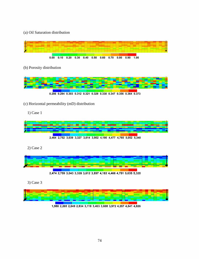
74

(a) Oil Saturation distribution

(b) Porosity distribution

(c) Horizontal permeability (mD) distribution

1) Case 1

2) Case 2

3) Case 3

75

4) Case 4

5) Case 5



spacing between the wells is equal to 50 m.

Case 3: In this case, a permeability distribution is created with same average permeability of

Cases 1 and 2, but with higher permeability at the upper zone and lower permeability at the

lower part of the reservoir, as displayed in Figure 4.1(e). The vertical permeability distribution of

this case would be expected where the sand grains are largest at the top of the reservoir and finest

at the base of the oil column.

Case 4: The permeability distribution for this case, shown in Figure 4.1(f), is created by scaling

up the permeabilities of the grid blocks of Case 1 universally by a factor of 2. This gives rise to

an average permeability of 7300 mD. This case represents the best permeability case examined

here and is at the upper limit of permeabilities expect in thin heavy oil reservoirs in Western

Canada.

76

Case 5: The permeability distribution of this case, displayed in Figure 4.1(g), is created by

scaling down the permeabilities of the grid blocks of Case 1 universally by a factor equal to 0.6.

This gives rise to an average permeability equal to 2190 mD. This case represents the worst

permeability case evaluated in this study.

For each of above reservoir model cases, an individual optimization of 800 runs was conducted

to determine the optimum parameter set for each case. The optimization run and simulations

were executed on a personal computer (3.4 GHz, dual quad core with 16 GB memory). Each

individual reservoir simulation took on average 2 min and 30 s to execute; given that 800

simulation runs were done each case, each optimization run took roughly 34 h to complete.

4.3.2 Optimization Algorithm

4.3.2.1 The Simulated Annealing Method

In this work, a Simulated Annealing (SA) algorithm is used for operating strategy optimization

as described in Gates and Chakrabarty (2008). The optimization algorithm is designed to control

the thermal reservoir simulator and execute reservoir performance evaluations. Parameters for

reservoir simulation are generated by the SA algorithm and then used for generating the

simulation input file. Then a simulation run based on the newly generated input file is executed

by the reservoir simulator. Once the simulation is complete, a computer code is called to process

the reservoir simulation output data and evaluate the performance of the simulated strategy. The

evaluation results are then sent back to the optimizer to generate new parameter sets and the next

iteration of the optimization algorithm starts. In the optimization procedure, the SA algorithm

conducts random searches that attempt to lower the value of the cost function, i.e., the optimum

77

value of desired reservoir operating performance. The parameters of the SA algorithm were the

same as those used in previous studies (Gates and Chakrabarty, 2008).

4.3.2.2 Adjustable Parameters and Cost Function

For optimization, the adjustable parameters are the injection pressures and injection water

temperature over specified time intervals, summarized in Table 4.2. The pressure and

temperature sampled during the optimization run ensures that none of the pressure/temperature

combinations are below the steam saturation line. In other words, conditions are maintained such

that only subcooled water is injected into the reservoir. In total, ten pressure parameters with

base value of 3000 kPa and optimization range set equal to 2000–4200 kPa, and ten water

temperature parameters with base value equal to 120 °C and range 20–250 °C are used to

optimize the process.

Table 4.2: List of Optimization Parameters.

Parameter Onset Time

(months)

Base Value, Allowed Range

1 Injection Well Pressure 0 3,000 kPa, 2,0004,200 kPa










11 Injection water temperature 0 20250C










78

The cost function against which the adjustable parameters are optimized is a function of the net

present value (NPV). For the simple economic model used here, the following economic factors

are considered: initial capital investment (including well drilling and field equipment), operating

costs, fixed costs, variable costs, water treatment costs, and operating revenue. The following

assumptions formed the basis of our evaluation: well drilling cost and other initial investment

$2,500,000 (for a single well), discount rate of 10%, variable cost to be 10% of the operating

revenue, heavy oil price $80.00/bbl (Teare et al., 2012), natural gas price $4.4/GJ, thermal

efficiency equal to 0.75, and waste water treatment cost is $2.00/m3. The cost function (CF) is

formally defined as CF = (6 × 106 − NPV)/1 × 10

6. This indexes the value of the CF to range, in

general, between 0 and 10 with lower values of the CF being more optimal.


4.4.1 Injection Pressure and Water Temperature

Figure 4.2 shows the optimized injection pressure and water temperature for all the optimized

cases. For Case 1, the results reveal that the injection pressure remains relatively high, around

4000 kPa, throughout the majority of the operating life of the process although a lower injection

pressure (2500 kPa) period exists between 1.5 and 2 years of operation. The optimized injection

pressure for all the other cases generally remains high in the majority of the operating time

before water breakthrough although exhibit stochastic deviations. In Case 4, the high

permeability zone leads to earlier oil production compared to the other cases. The injecting

pressure remains high over the first two years and shows a cyclic pattern in the later stages of

operation. In Case 1, the initiate water temperature is found to be around 120 °C and then jump

79

to 225 °C for a period of 6 months. After this high water temperature period follows a low

injecting temperature period of 1.5 years with water temperature ranging from 20 to 50 °C. The

water temperature increases to 175 °C and is then further elevated to 250 °C after 3 years of

operation. The 250 °C injection period persists for a year before the temperature decreases to 94

°C and then finally to 20 °C for the last 14 months of operation. From Figure 4.2, one can see

that there is similar pattern for the optimized injecting water temperature. The water temperature

normally starts high and then gives rise to a low injection temperature period. We could call this

temperature change from high to low an injection cycle. In the 5 cases investigated here, the

second cycle tends to last longer than the first cycle. In Case 5 as shown in Figure 4.2e, a third

cycle occurs within the six year operation life.

(a) Case 1

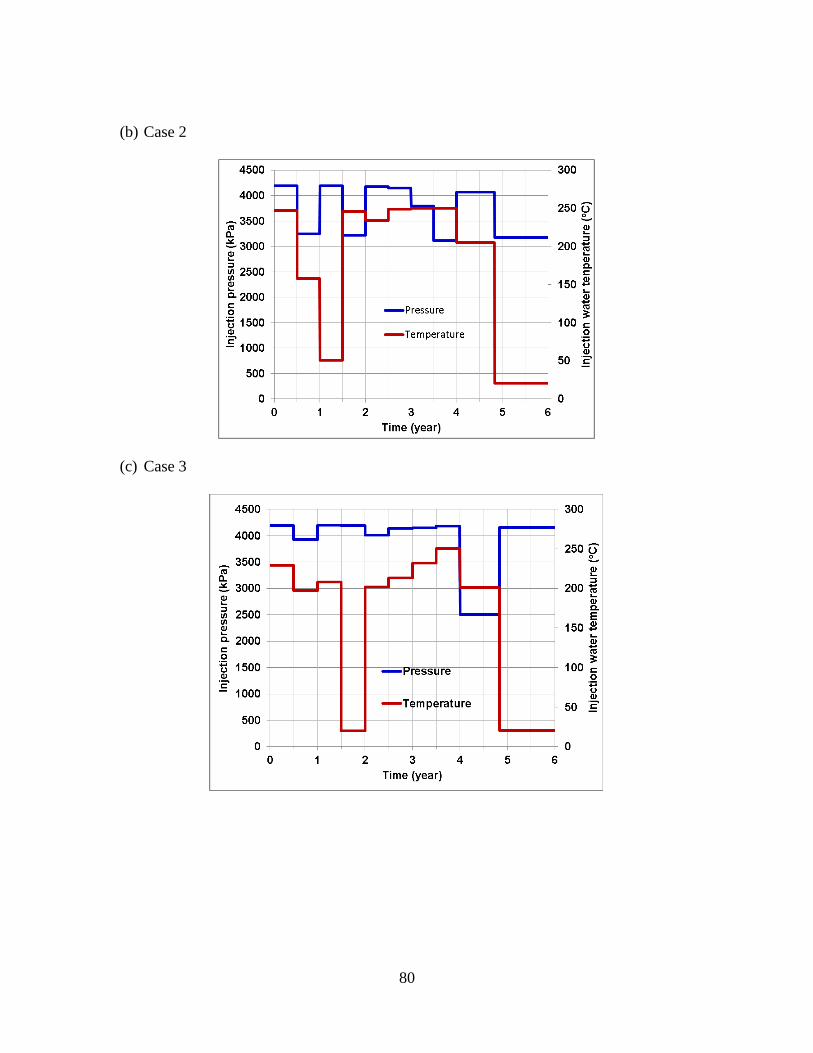
80

(b) Case 2

(c) Case 3

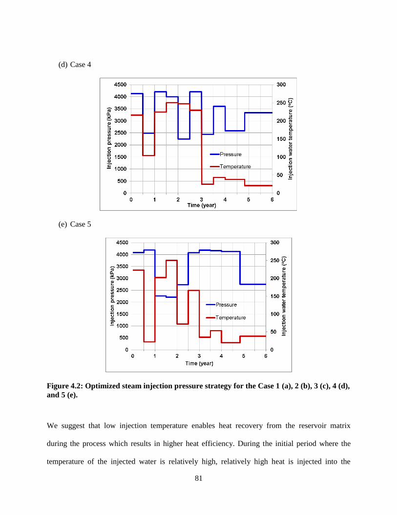
81

(d) Case 4

(e) Case 5

Figure 4.2: Optimized steam injection pressure strategy for the Case 1 (a), 2 (b), 3 (c), 4 (d),

and 5 (e).

We suggest that low injection temperature enables heat recovery from the reservoir matrix

during the process which results in higher heat efficiency. During the initial period where the

temperature of the injected water is relatively high, relatively high heat is injected into the

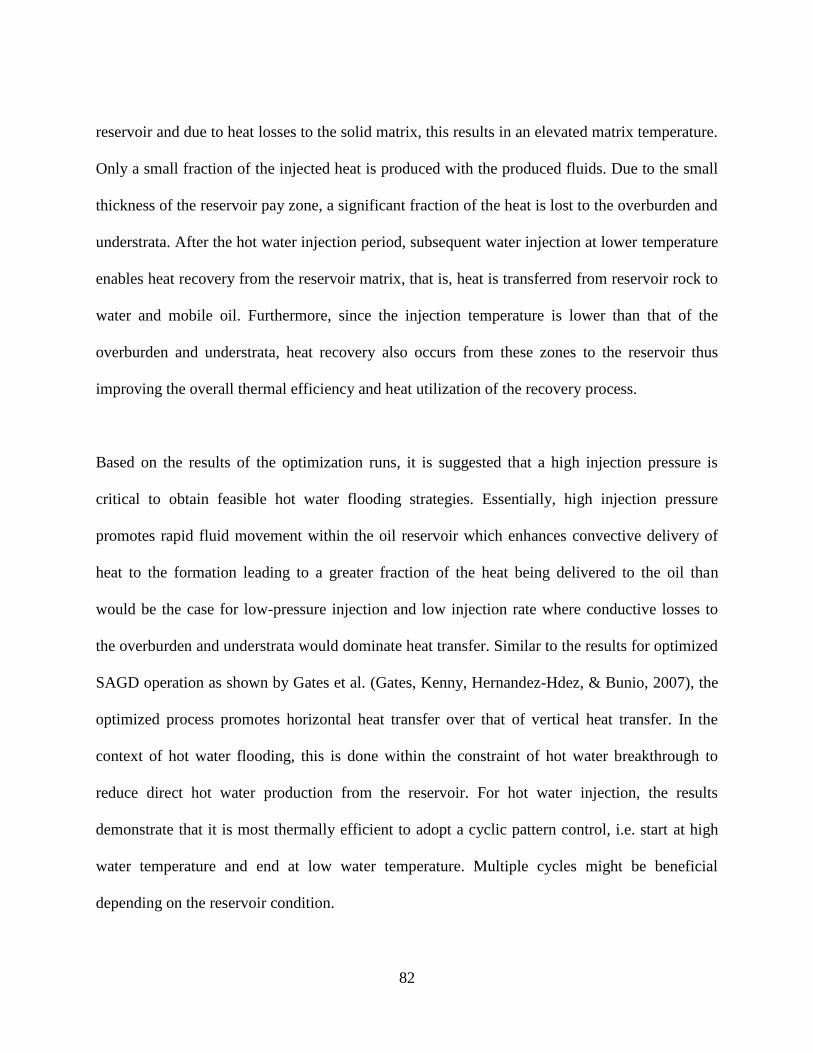
82

reservoir and due to heat losses to the solid matrix, this results in an elevated matrix temperature.

Only a small fraction of the injected heat is produced with the produced fluids. Due to the small

thickness of the reservoir pay zone, a significant fraction of the heat is lost to the overburden and

understrata. After the hot water injection period, subsequent water injection at lower temperature

enables heat recovery from the reservoir matrix, that is, heat is transferred from reservoir rock to

water and mobile oil. Furthermore, since the injection temperature is lower than that of the

overburden and understrata, heat recovery also occurs from these zones to the reservoir thus

improving the overall thermal efficiency and heat utilization of the recovery process.

Based on the results of the optimization runs, it is suggested that a high injection pressure is

critical to obtain feasible hot water flooding strategies. Essentially, high injection pressure

promotes rapid fluid movement within the oil reservoir which enhances convective delivery of

heat to the formation leading to a greater fraction of the heat being delivered to the oil than

would be the case for low-pressure injection and low injection rate where conductive losses to

the overburden and understrata would dominate heat transfer. Similar to the results for optimized

SAGD operation as shown by Gates et al. (Gates, Kenny, Hernandez-Hdez, & Bunio, 2007), the

optimized process promotes horizontal heat transfer over that of vertical heat transfer. In the

context of hot water flooding, this is done within the constraint of hot water breakthrough to

reduce direct hot water production from the reservoir. For hot water injection, the results

demonstrate that it is most thermally efficient to adopt a cyclic pattern control, i.e. start at high

water temperature and end at low water temperature. Multiple cycles might be beneficial

depending on the reservoir condition.

83

4.4.2 Oil Production Rates and Effects of Permeability Variations

Figure 4.3 shows the oil production rates for Cases 1–5. The peak oil production rates are found

to range from 20 to 25 m3/day for Cases 1–4. In Case 5, the maximum oil rate seldom exceeds 5

m3/day. The results show that despite the same average permeability value, the distribution of the

permeability within the pay zone impacts oil production. In Case 2, a higher permeability zone is

located at the bottom zone of the reservoir. This results in earlier oil production than that of Case

3, the case where a higher permeability zone is located at the upper part of the reservoir. The

higher permeability at the lower part of the reservoir causes faster hot water frontal advance in

the lower part of the reservoir. This enhances heat transfer (tends to migrate upwards rather than

downwards) to the oil above the higher permeability zone at the base of the reservoir.

Furthermore, the accelerated water front speed leads to more oil displacement and production.

As listed in Table 3, within the same operating time of 6 years, Case 2 produced 3% more oil

than Case 3. On the other hand, 11% more water is produced in the optimized Case 2, which is

caused by the higher permeability of the lower region of pay zone. Case 3 produces 5% more oil

than Case 1 but used 40% more heat injection over the total 6 years of operation. The higher

permeability interval at the upper part of reservoir contributes to larger heat losses to the

overburden.

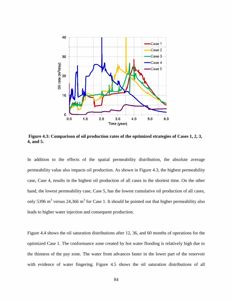
84

Figure 4.3: Comparison of oil production rates of the optimized strategies of Cases 1, 2, 3,

4, and 5.

In addition to the effects of the spatial permeability distribution, the absolute average

permeability value also impacts oil production. As shown in Figure 4.3, the highest permeability

case, Case 4, results in the highest oil production of all cases in the shortest time. On the other

hand, the lowest permeability case, Case 5, has the lowest cumulative oil production of all cases,

only 5396 m3 versus 24,366 m

3 for Case 1. It should be pointed out that higher permeability also

leads to higher water injection and consequent production.

Figure 4.4 shows the oil saturation distributions after 12, 36, and 60 months of operations for the

optimized Case 1. The conformance zone created by hot water flooding is relatively high due to

the thinness of the pay zone. The water front advances faster in the lower part of the reservoir

with evidence of water fingering. Figure 4.5 shows the oil saturation distributions of all

85

optimized cases after 4 years of operation. In Case 2, as shown in Figure 4.5b, due to higher

permeability at the lower part of the reservoir, the water front moves much faster in the lower

part and breaks through at an early time which lead to overall higher water cut. In Case 3, as

shown in Figure 4.5c, the advance of the water front is relatively uniform in the pay zone. In

Case 4, the high permeability is found to result in lowest oil saturation after 4 years of operation

(Figure 4.5d). However, in Case 5 (Figure 4.5e), due to the low permeability, the water front

moves at a relatively slow pace which resulted in the lowest oil production.

(a) after 12 months

(b) after 36 months

(c) after 60 months

Figure 4.4: Oil saturation profiles of optimized Case 1.

86

Case 1

Case 2

Case 3

Case 4

Case 5

Figure 4.5: Oil saturation distributions after 4 years of operation for Cases 1, 2, 3, 4, and 5.

4.4.3 Water Injection rates and Water Production

The water injection rates in all the optimized cases are shown in Figure 4.6. For Cases 1–3, the

initial water injection rates are generally low in the early stages of oil production but ramp up as

the operation continues. Since the injection temperature drops as the operations progress, at the

later stage of hot water flooding, water breakthrough does not cause substantial heat losses since

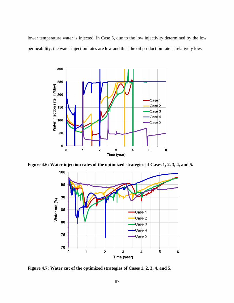
87

lower temperature water is injected. In Case 5, due to the low injectivity determined by the low

permeability, the water injection rates are low and thus the oil production rate is relatively low.

Figure 4.6: Water injection rates of the optimized strategies of Cases 1, 2, 3, 4, and 5.

Figure 4.7: Water cut of the optimized strategies of Cases 1, 2, 3, 4, and 5.

88

Figure 4.7 shows the water cut of all of the cases studied here. The water cuts are generally

larger than 80%. At the later stages, water cuts rise to above 95%. In Case 4 where reservoir has

the largest permeability, the water cut rises to 99% by the end of the 6 years of operation.

4.4.4 Temperature distributions, cumulative energy injected to oil ratio (cEOR), and net

present value

(a) After 12 months of operation

(b) After 36 months of operation

(c) After 60 months of operation

Figure 4.8: (a) - (c) Temperature (C) distributions of optimized Case 1.

Figure 4.8 presents the spatial distributions of the temperature after 12, 36, and 60 months of

operation in the optimized Case 1. Figure 4.9, Figure 4.10, Figure 4.11 and Figure 4.12 present

the temperature distributions after 12, 36, and 60 months in optimized Cases 2–5. In Case 1, the

reservoir temperature peaks at about 100 °C by the end of high temperature water injection

period (at the end of 4 years of operation). Due to the use of cold water for injection, the

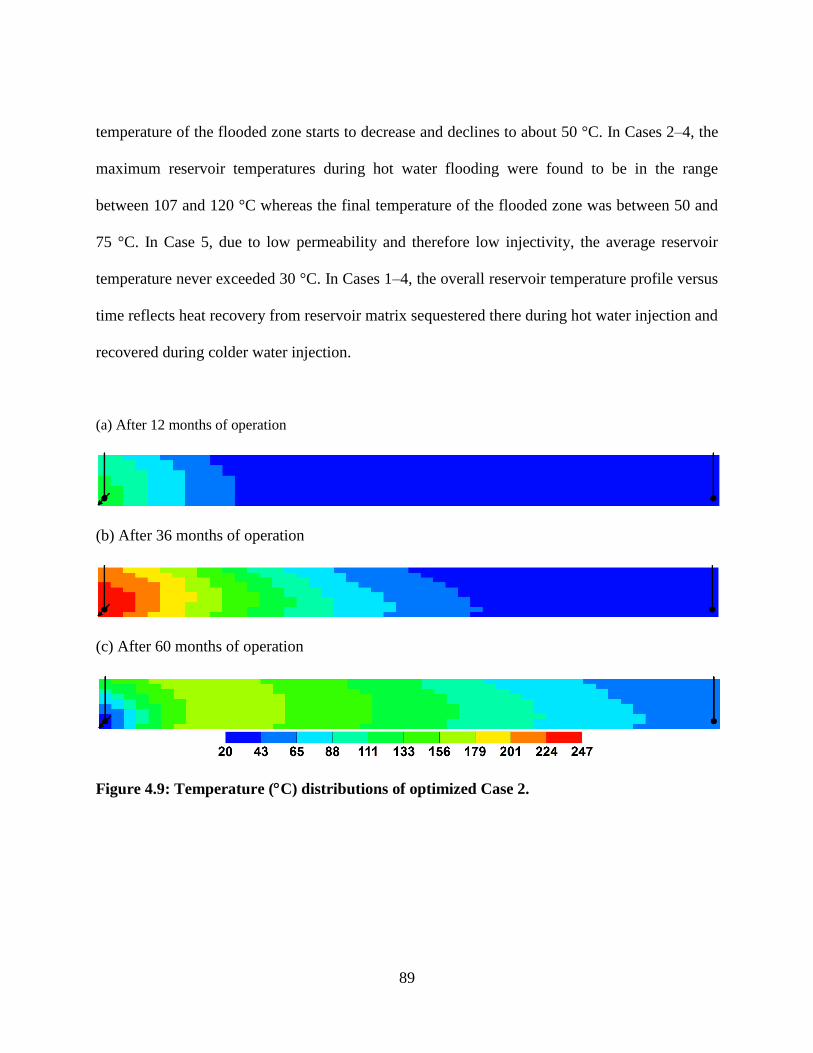
89

temperature of the flooded zone starts to decrease and declines to about 50 °C. In Cases 2–4, the

maximum reservoir temperatures during hot water flooding were found to be in the range

between 107 and 120 °C whereas the final temperature of the flooded zone was between 50 and

75 °C. In Case 5, due to low permeability and therefore low injectivity, the average reservoir

temperature never exceeded 30 °C. In Cases 1–4, the overall reservoir temperature profile versus

time reflects heat recovery from reservoir matrix sequestered there during hot water injection and

recovered during colder water injection.




Figure 4.9: Temperature (C) distributions of optimized Case 2.

90









91








(NPV).

Case

Cumulative oil

production (m3)

cWOR

(m3/m

3)

cEOR

(GJ/m3)

NPV*

($million)

1 24,366 14.5 6.2 2.8

2 26,400 14.6 9.9 2.9

3 25,655 13.5 8.2 2.9

4 27,319 19.1 7.4 4.7

5 5,396 13.7 3.4 -1.6 *The blowdown performance is not considered in the NPV calculation which means the real NPV could be slightly

higher than the presented values.

92

The cumulative energy injected (as sensible heat in the injected water) to produced oil ratio

(cEOR, expressed as GJ injected energy per m3 of oil produced) versus time for all the cases is

displayed in Figure 4.13 with results at the end of the six years of operation listed in Table 4.3.

The cEOR generally starts high due to heat losses and initial low oil production rate. As the oil

rate increases, the cEOR decreases. By the end of the high oil production rate period, the cEOR

increases until cold-water injection is started which then recovers heat previously stored in the

reservoir matrix. In Case 1, the resulting cEOR is equal to 6.2 GJ/m3, being the lowest value

excluding Case 5. In Case 2, the existence of the high permeability layer in the lower part of

reservoir results in relatively early water break through and therefore greater energy injection,

more heat losses to overburden, a higher overall reservoir temperature (Figure 4.14), and the

highest cEOR equal to 9.9 GJ/m3. Case 5 achieved the lowest cEOR but also resulted in the

lowest production rate and recovered oil volume and therefore had a negative net present value

(NPV). This result suggests that heat losses were reduced in the low permeability case but oil

production suffers resulting in an uneconomic process. Of the five cases studied, the resulting

overall cEOR after six years of operation is under 10 GJ/m3, which indicates relatively good heat

utilization efficiency. The calculated NPV reveals that hot water flooding, with the economic

inputs used here, can be economic in thin (<6 m) heavy oil reservoirs with the base case (Case 1)

properties and that high and low permeability zones at the top or bottom of the reservoir realize

similar NPV providing the overall permeability is similar. The results show that Case 4 achieved

the best economic outcome of the cases studied here – this is a result of its enhanced

permeability.

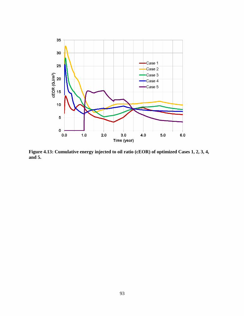
93

Figure 4.13: Cumulative energy injected to oil ratio (cEOR) of optimized Cases 1, 2, 3, 4,

and 5.

94

Figure 4.14: Average reservoir temperature as function of operating time in optimized

Cases 1, 2, 3, 4, and 5.

4.5 Conclusions

In the present work, stochastic optimization was conducted to determine the optimum injecting

pressure and injecting water temperature strategies in thin heavy oil reservoir in five cases. The

key results are as follows.

A high injecting pressure is critical to a success hot water flooding strategy. In the present

optimized cases, the injection pressures remain high during the operating process although

deviations present. This promotes larger horizontal heat transfer (convective) than vertical

95

heat losses (vertical losses adversely impact process performance due to heat losses to non-

productive overburden and understrata).

For water injection, the results suggest that starting with high temperature injection to lower

temperature injection later on provides opportunities to recover heat from the reservoir and

overburden and understrata thus improving the thermal efficiency of the process. Multiple

cycles of high/low temperature water injection might be beneficial depending on the

reservoir condition.

The permeability distribution is found to affect the performance of the hot water flooding

process. The existence of higher permeability zone at the lower part of the reservoir leads to

earlier oil production and water breakthrough. The higher injectivity and water production

also caused higher cEOR. The performance of Case 3, which has higher permeability zone at

upper part of the reservoir, is comparable to that of the Case 1 but it used 40% more heat

injection.

The absolute overall permeability of the reservoir impacts performance significantly. Case 4

produced the largest amount of oil and water in the early stage of operation. Although Case

4’s produced water-to-oil is also substantially higher than the other cases, it achieved the best

economic performance. The low permeability of Case 5 led to slow oil production. Although

it has the lowest cEOR, the poor oil production made the operation process uneconomic.

4.6 References





96



Diaz-Munoz, J., & Farouq Ali, S. M. (1975). Simulation of Cyclic Hot Water Stimuation of

Heavy Oil Wells.



Gates, I. D. (2010). Solvent-aided Steam-Assisted Gravity Drainage in Thin Oil Sand Reservoirs.

J Petrol Sci Eng, 74, 138-146.


Gates, I. D., & Chakrabarty, N. (2008). Design of the steam and Solvent Injection Strategy in

Expanding Solvent Steam-Assisted Gravity Drainage. J Can Petrol Technol, 47, 12-20.

Gates, I. D., Kenny, J., Hernandez-Hdez, I. L., & Bunio, G. L. (2007). Steam Injection Strategy

and Energetics of Steam-Assisted Gravity Drainage. SPE Reserv Eval Eng, 10, 19-34.

Istchenko, C., & Gates, I. D. (2014). Well-wormhole model of cold heavy oil production with

sand. SPE Journal, 19(2), 260-269.



Martin, W. L., Dew, J. N., Powers, M. L., & Steves, H. B. (1967). Results of a Teriary Hot

Waterflood in a Thin Sand Reservoir. J Can Petrol Technol, 243, 739-750.









2012–2021.

Vinsome, P. K. W., & Westerveld, J. D. (1980). A simple method for predicting cap and base

rock heat losses in thermal reservoir simulators. Journal of Canadian Petroleum

Technology, 19, 87-90.

Zhao, W., Wang, J., & Gates, I. D. (2014). Thermal recovery strategies for thin heavy oil

reservoirs Fuel, 117, 431-441.

97

CHAPTER FIVE: OPTIMIZED SOLVENT-AIDED STEAM-FLOODING STRATEGY

FOR RECOVERY OF THIN HEAVY OIL RESERVOIRS


citation is as follows: Zhao, W., Wang, J., and Gates, I.D. Optimized Solvent-aided Steam-

flooding Strategy for Recovery of Thin Heavy Oil Reservoirs. Fuel, 112:50-59, 2013.

5.1 Abstract

Stochastic optimization based on a simulated annealing method was carried out to determine the

optimum steam and steam–solvent flooding strategies in a thin (4 m) heavy oil reservoir both in

the absence and presence of a bottom water zone. The steam injection pressure optimization case

determined a technically feasible operating strategy. However, the cumulative energy to

produced oil ratio (cEOR) realized from the optimized process is high. In comparison, the

solvent-aided steam optimization case achieved an operating strategy with a much lower cEOR

and cumulative water-to-oil ratio (cWOR) than those in the optimized injection pressure-only

strategy. We observed that a solvent-rich channel forms at the top of the reservoir after solvent

breakthrough occurs at the production well. The formation of the solvent-rich channel led to oil–

solvent mixing at the periphery of the channel as well as heat transfer to oil beyond the channel,

which in turn resulted in better recovery performance. In the presence of a bottom water zone,

the optimized steam injection pressure optimization strategy was found to perform poorly.

However, the optimized solvent-aided strategy achieved superior performance. With solvent

injection, the presence of the bottom water zone enhanced mixing of solvent and oil yielding

improved oil recovery performance.

98

5.2 Introduction

Although currently commercial thermal-based techniques such as Steam-Assisted Gravity

Drainage (SAGD) and Cyclic Steam Stimulation (CSS) are successful for recovering bitumen

and heavy oil from thick pay zones (>15 m), their application in thin heavy oil (<6 m) reservoirs

are generally not thought to be economically viable. This is due to the high steam-to-oil ratio

(SOR) caused by significant heat losses to the overburden relative the amount of heat delivered

to the oil which renders the processes uneconomic. Heavy oil cold production (CP) employs

small energy input. However, the average recovery factor is typically low, usually, between 3%

and 8% of the Original Oil In Place (OOIP) (Adams, 1982). By employing the so called Cold

Heavy Oil Production with Sand (CHOPS) technique, the recovery factor can reach as high as

15% (Pan et al., 2010). However, the formation of wormholes during CHOPS operation creates

new challenges for applying follow-up processes to recover additional oil beyond CHOPS.

In conventional oil reservoirs, water flooding and polymer flooding have been the most widely

used techniques for secondary recovery after the end of primary production (Asghari &

Nakutnyym, 2008; Miller, 2005). For heavy oil reservoirs, however, the performance of both

water flooding and polymer strategy are poorer and commercially successful cases are mostly

found for reservoirs with dead oil viscosities less than a few thousand cP (Asghari &

Nakutnyym, 2008; Gao, 2011; Miller, 2005).

Existing thermal-based recovery process studies based on laboratory experiments, field trials, or

reservoir simulation of thin heavy oil (<50,000 cP) reservoirs are rare. Stalder (Stalder, 2009)

reported reservoir simulation results on the application of Cross Steam-Assisted Gravity

99

Drainage (XSAGD) for a bitumen reservoir with a net pay of 10 m. The results demonstrated

that there are economic advantages of XSAGD over SAGD. However, despite improved

performance beyond that of SAGD, he stated that it is not economic to apply XSAGD to thinner

reservoirs. Tavallali et al. (Tavallali, Maini, & Harding, 2012) reported on the results of

optimizing the SAGD well configuration in a 10 m thick Lloydminster-type heavy oil reservoir

with a dead oil viscosity of 5000 cP. They suggested that placing the production well offset from

the injection well is the optimum well configuration for depleting the reservoir in the shortest

period of time.

Solvent injection based recovery methods for bitumen and heavy oil have attracted increasing

attention in recent years. Gates (Gates, 2010) proposed a solvent-aided thermal recovery process

for 8 m thick oil sands reservoir. Gates reported that the solvent-aided process led to

substantially lower steam usage and net injected energy (both steam and solvent lost to the

reservoir) to oil ratio compared to that with traditional SAGD. Istchenko (Istchenko, 2012)

examined a cyclic solvent process as a potential technique for post-CHOPS field operation. The

results suggested that the overall recovery factor could be raised by about 50%.

However, to the best of our knowledge, studies to understand and design solvent-aided thermal

recovery processes for heavy oil reservoirs with thickness less than 5 m have not been done

before. Here, to better understand and to derive viable thermal recovery process designs for

extracting oil from thin (<5 m) heavy oil reservoirs, a reservoir simulation study has been done

to investigate steam-based recovery processes with and without solvent.

100

5.3 Reservoir Simulation Model

The reservoir model, solved in a commercial thermal reservoir simulator (Computer Modeling

Group Ltd, 2012), is a two-dimensional model with two horizontal wells spaced 50 m apart as

used in a previous study (Zhao et al., 2012). A detailed listing of the underlying equations, finite

volume discretization, and solution algorithms is described in CMG (Computer Modeling Group

Ltd, 2012). The thickness of the heavy oil interval is equal to 4 m. The models were discretized

into a regular Cartesian grid with dimensions 1 m in the cross-well direction, 1000 m in the

downwell direction, and 0.4 m in the vertical direction resulting in 500 grid blocks in the model.

The length of the perforated intervals of the horizontal wells in all models is equal to 1000 m.

The reservoir simulation model and fluid properties are listed in Table 4.1.

The spatial distributions of porosity (average equal to 0.32), horizontal permeability (average

equal to 3650 mD), and oil/water saturations (average oil saturation equal to 0.65), displayed in

Figure 5.1, were derived from core data taken from one of Devon Canada’s heavy oil fields

located in eastern Alberta. The vertical-to-horizontal permeability ratio is equal to 0.8. The initial

reservoir pressure and temperature are equal to 2800 kPa and 20 °C, respectively. The solution

gas-to-oil ratio at original reservoir conditions is equal to 6.17 m3/m

3. All reservoir simulation

models were run in parallel on a 12-core personal computer; a typical simulation took roughly 10

min to execute.

101

(a) Oil Saturation distribution

(b) Porosity distribution

(c) Horizontal permeability (mD) distribution



spacing between the wells is equal to 50 m.

5.4 Optimization Algorithm

5.4.1 The simulated annealing method

In this work, a simulated annealing (SA) algorithm is used for operating strategy optimization

following that of Gates (Gates, 2010). As a random search technique, the simulated annealing

method was first proposed by Metropolis et al. (Metropolis, Rosenbluth, Rosenbluth, Teller, &

Teller, 1953) for atomistic simulation and has been used for reservoir simulation optimization.

The optimization algorithm is wrapped around and controls the thermal reservoir simulator.

Parameters for reservoir simulation are generated by the SA algorithm and then used for

assembling the simulation input file. Then a simulation run based on the newly generated input

file is performed by the reservoir simulator. Once the simulation is complete, a computer code is

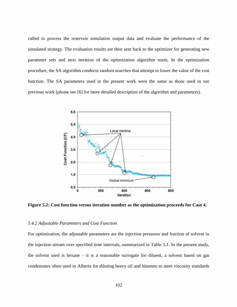
102

called to process the reservoir simulation output data and evaluate the performance of the

simulated strategy. The evaluation results are then sent back to the optimizer for generating new

parameter sets and next iteration of the optimization algorithm starts. In the optimization

procedure, the SA algorithm conducts random searches that attempt to lower the value of the cost

function. The SA parameters used in the present work were the same as those used in our

previous work (please see [6] for more detailed description of the algorithm and parameters).

Figure 5.2: Cost function versus iteration number as the optimization proceeds for Case 4.

5.4.2 Adjustable Parameters and Cost Function

For optimization, the adjustable parameters are the injection pressures and fraction of solvent in

the injection stream over specified time intervals, summarized in Table 5.1. In the present study,

the solvent used is hexane – it is a reasonable surrogate for diluent, a solvent based on gas

condensates often used in Alberta for diluting heavy oil and bitumen to meet viscosity standards

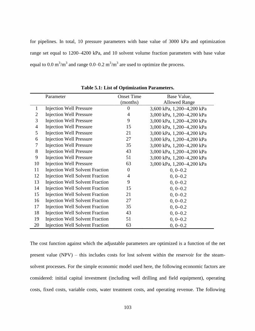
103

for pipelines. In total, 10 pressure parameters with base value of 3000 kPa and optimization

range set equal to 1200–4200 kPa, and 10 solvent volume fraction parameters with base value

equal to 0.0 m3/m

3 and range 0.0–0.2 m

3/m

3 are used to optimize the process.

Table 5.1: List of Optimization Parameters.

Parameter Onset Time

(months)

Base Value,

Allowed Range











11 Injection Well Solvent Fraction 0 0, 00.2










The cost function against which the adjustable parameters are optimized is a function of the net

present value (NPV) – this includes costs for lost solvent within the reservoir for the steam-

solvent processes. For the simple economic model used here, the following economic factors are

considered: initial capital investment (including well drilling and field equipment), operating

costs, fixed costs, variable costs, water treatment costs, and operating revenue. The following

104

assumptions formed the basis of our evaluation: well drilling cost and other initial investment

$2,500,000 (for a single well), discount rate of 10%, variable cost to be 10% of the operating

revenue, heavy oil price $80.00/bbl (Teare et al., 2012), natural gas price $4.4/GJ, thermal

efficiency equal to 0.75, solvent price $95.00/bbl, and waste water treatment cost is $2.00/m3.

Then the cost function (CF) is formally defined as: CF = (7 × 106 – NPV)/1 × 10

6. This indexes

the value of the CF to range, in general, between 0 and 10 with lower values of the CF being

more optimal. The optimum operating strategy is chosen as the case with the lowest CF among

all of the cases executed. An example of the evolution of the cost function for Case 4 (described

below) versus iteration number is displayed in Figure 5.2. The results demonstrate that the SA

algorithm is capable of stepping out of local minima to seek out the global minimum.

5.5 Details of investigated cases for optimization

5.5.1 Steam injection pressure optimization

In this case, only steam injection pressures are taken as target for optimization. Both the injection

and production well is located 0.6 m above the reservoir bottom.

5.5.2 Steam injection pressure and solvent fraction optimization

In this case, the reservoir model and well configurations are identical to those in Case 1. The

parameters for optimization are the steam injection pressure and solvent volume fraction in the

injection steam.

5.5.3 Steam injection pressure optimization in the presence of 2 m bottom water zone

In the present case, the reservoir model is derived from Case 1 by adding a 2-m thick bottom

water zone (water saturation is 1.0 in this region). Both the injection and production well are

105

located 1.4 m above the water zone. Only steam injection pressure is optimized (no solvent

injection is used).

5.5.4 Steam injection pressure and solvent fraction optimization in the presence of 2 m bottom

water zone

In the present case, the reservoir model and well configuration are identical to that of Case 3.

Both steam injection pressure and solvent volume fraction are optimized to achieve the best

operating strategy.

In all the above cases, the production wells are subject to two constraints: first, a bottom hole

pressure of 500 kPa and a total maximum liquid production rate equal to 500 m3 per day. The

total number of reservoir simulations executions that were conducted was equal to 800 in each

optimization run – the optimal solution was the best one achieved among the 800 runs. The

optimized strategies are further improved by adopting a two to three-month blowdown period at

the point of time when maximum NPV is achieved.


5.6.1 Steam injection pressure optimization.

Figure 5.3 shows the optimized steam injection pressure operating strategy. The optimized

strategy yielded a maximum NPV after 73 months. In the best case, the pressure started at 3300

kPa and stepped up to 4200 kPa before it bottomed at 2275 kPa. Thereafter, the pressure

increased to 4200 kPa and then dropped down to 3300 kPa at the end of the 73-month operating

period. As shown in Table 5.2, the optimized strategy achieved a cumulative oil production of

32,278 m3 (recovery factor equal to 77%) with a cWOR equal to 7.0 m

3/m

3. The cumulative

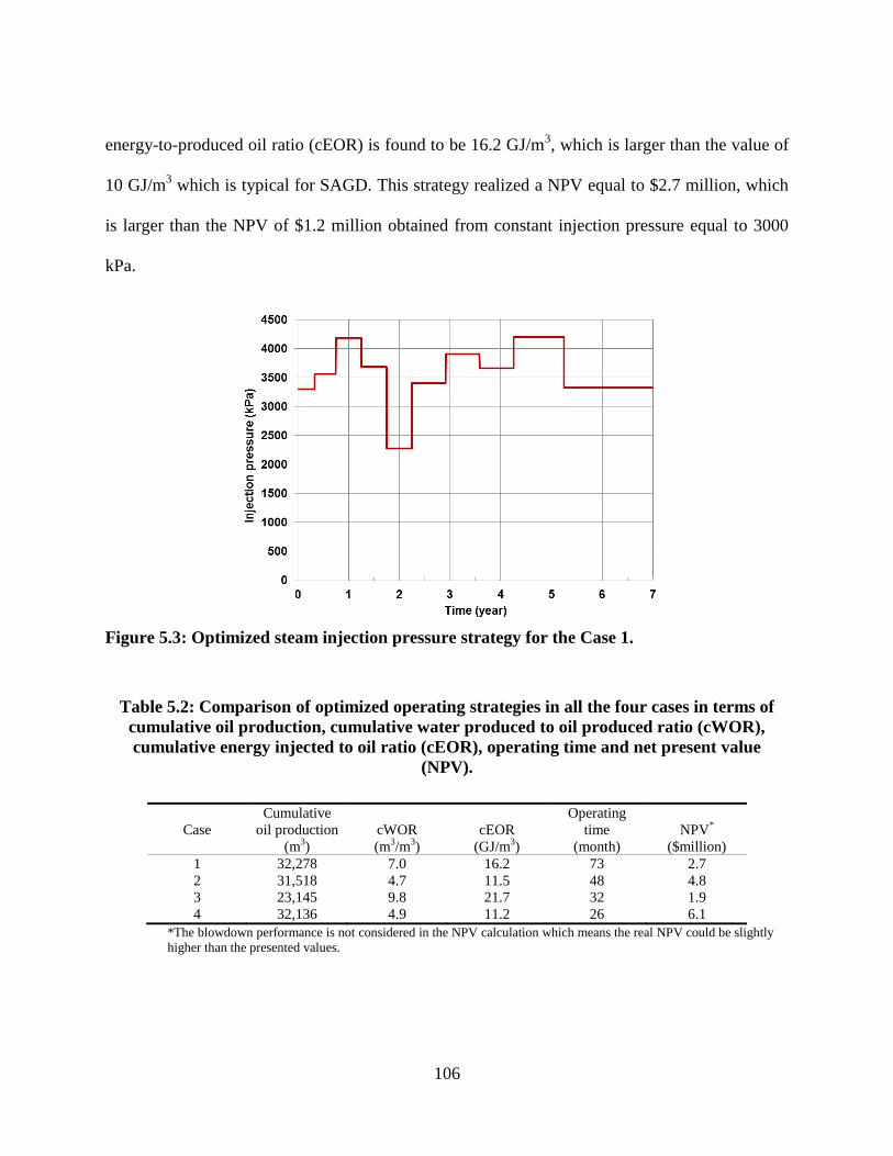
106

energy-to-produced oil ratio (cEOR) is found to be 16.2 GJ/m3, which is larger than the value of

10 GJ/m3 which is typical for SAGD. This strategy realized a NPV equal to $2.7 million, which

is larger than the NPV of $1.2 million obtained from constant injection pressure equal to 3000

kPa.

Figure 5.3: Optimized steam injection pressure strategy for the Case 1.




(NPV).

Case

Cumulative

oil production

(m3)

cWOR

(m3/m

3)

cEOR

(GJ/m3)

Operating

time

(month)

NPV*

($million)

1 32,278 7.0 16.2 73 2.7

2 31,518 4.7 11.5 48 4.8

3 23,145 9.8 21.7 32 1.9

4 32,136 4.9 11.2 26 6.1

*The blowdown performance is not considered in the NPV calculation which means the real NPV could be slightly

higher than the presented values.

107

Figure 5.4: Optimized steam injection pressure and solvent fraction for the Case 2.

5.6.2 Case 2. Steam injection pressure and solvent fraction optimization.

Figure 5.4 shows the optimized strategy employing both steam and solvent injection for this

case. The optimized strategy realized a maximum NPV after 48 months. The results of this case

are different from that of Case 1. Here, the pressure started with relatively low values ranging

from 1500 to 2600 kPa over the first 21 months. It then increased to between 3800 and 4200 kPa

over the next 14 months, which was followed by a substantial pressure reduction to 1200 kPa,

which then remained for the last 13 months of its total 48-month operating time. The solvent

injection strategy exhibited a cyclic pattern with relative higher value (0.14–0.20 m3/m

3) during

the period of 10th to 27th month and a much lower value of 0.007 m3/m

3 for its last 5 months.

108

Figure 5.5: Comparison of oil production rates and cumulative oil production of the

optimized strategies of the Case 1 (pressure) and Case 2 (pressure +solvent).

The optimized strategy of Case 2 realized a cumulative oil production equal to 31,518 m3

(recovery factor equal to 75%), which is similar to that in the Case 1. However, it depleted the

reservoir in about 48 months, a 34% reduction in operating time. Figure 5.5 shows the oil

production rates of the optimized strategies of the Cases 1 and 2. Although the optimized

strategy of the Case 2 underperformed that of the Case 1 in terms of oil production rate over the

first 2 years of operation, it achieved much higher oil rates over the next 2 years. It also achieved

relatively low WOR (4.7 m3/m

3). As shown in Figure 5.6, the cEOR of the Case 2 optimized

strategy is high over the first 2 years. This is due to low oil production rate during the same

period while solvent injection was employed (solvent injected but not produced is considered to

be energy injection cost). With high oil rates in the next 2 year, the cEOR quickly decreased and

ended up with an overall value of 11.5 GJ/m3, which is better than that of Case 1 and comparable

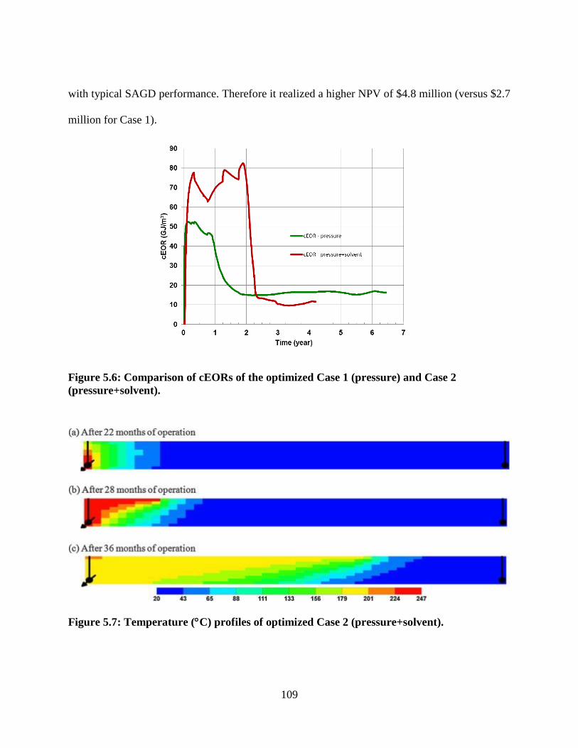
109

with typical SAGD performance. Therefore it realized a higher NPV of $4.8 million (versus $2.7

million for Case 1).

Figure 5.6: Comparison of cEORs of the optimized Case 1 (pressure) and Case 2

(pressure+solvent).

Figure 5.7: Temperature (C) profiles of optimized Case 2 (pressure+solvent).

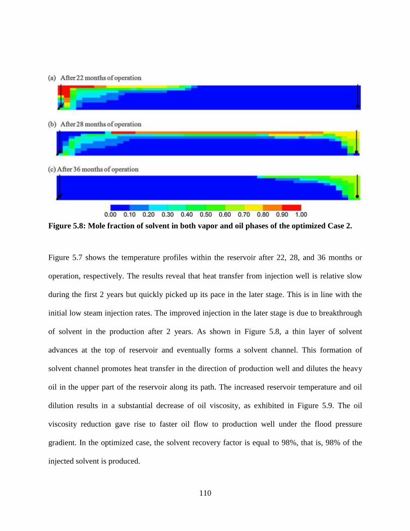
110

Figure 5.8: Mole fraction of solvent in both vapor and oil phases of the optimized Case 2.

Figure 5.7 shows the temperature profiles within the reservoir after 22, 28, and 36 months or

operation, respectively. The results reveal that heat transfer from injection well is relative slow

during the first 2 years but quickly picked up its pace in the later stage. This is in line with the

initial low steam injection rates. The improved injection in the later stage is due to breakthrough

of solvent in the production after 2 years. As shown in Figure 5.8, a thin layer of solvent

advances at the top of reservoir and eventually forms a solvent channel. This formation of

solvent channel promotes heat transfer in the direction of production well and dilutes the heavy

oil in the upper part of the reservoir along its path. The increased reservoir temperature and oil

dilution results in a substantial decrease of oil viscosity, as exhibited in Figure 5.9. The oil

viscosity reduction gave rise to faster oil flow to production well under the flood pressure

gradient. In the optimized case, the solvent recovery factor is equal to 98%, that is, 98% of the

injected solvent is produced.

111

Figure 5.9: Viscosity (cP) profile of the optimized Case 2 (the grid blocks shown in white

represent region with viscosity less than 1 cP).

5.6.3 Steam injection pressure optimization in the presence of 2 meter bottom water zone.

The optimized operating strategy achieved maximum NPV after 32 months of operation. The

optimized steam injection pressure for this case is displayed in Figure 5.10. The injection

pressure started at about 2700 kPa and then increased in a stepwise manner to 3900 kPa and

remained in the range from 3700 to 3900 kPa for 16 months. At the last one third of the total 32-

month operating time (approximately 11 months), the injection pressure was equal to about 1200

kPa.

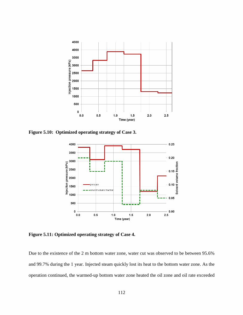
112

Figure 5.10: Optimized operating strategy of Case 3.

Figure 5.11: Optimized operating strategy of Case 4.

Due to the existence of the 2 m bottom water zone, water cut was observed to be between 95.6%

and 99.7% during the 1 year. Injected steam quickly lost its heat to the bottom water zone. As the

operation continued, the warmed-up bottom water zone heated the oil zone and oil rate exceeded

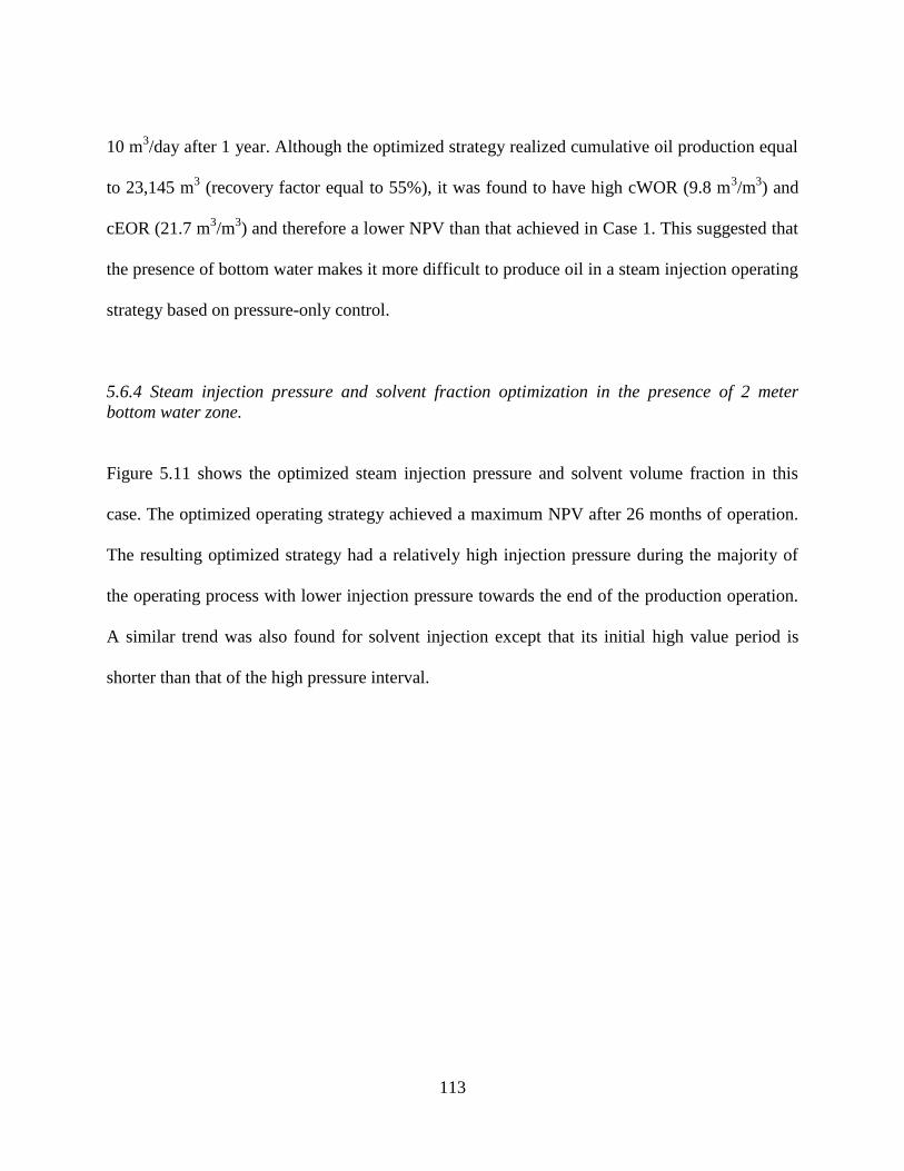
113

10 m3/day after 1 year. Although the optimized strategy realized cumulative oil production equal

to 23,145 m3 (recovery factor equal to 55%), it was found to have high cWOR (9.8 m

3/m

3) and

cEOR (21.7 m3/m

3) and therefore a lower NPV than that achieved in Case 1. This suggested that

the presence of bottom water makes it more difficult to produce oil in a steam injection operating

strategy based on pressure-only control.

5.6.4 Steam injection pressure and solvent fraction optimization in the presence of 2 meter

bottom water zone.

Figure 5.11 shows the optimized steam injection pressure and solvent volume fraction in this

case. The optimized operating strategy achieved a maximum NPV after 26 months of operation.

The resulting optimized strategy had a relatively high injection pressure during the majority of

the operating process with lower injection pressure towards the end of the production operation.

A similar trend was also found for solvent injection except that its initial high value period is

shorter than that of the high pressure interval.

114

Figure 5.12: Oil production rate and cumulative oil production of optimized Case 3

(pressure) and Case 4 (pressure+solvent).

As shown in Figure 5.12, the optimized case yielded a cumulative oil production volume equal to

32,137 m3 (recovery factor equal to 77%), a 39% increase compared to that of the optimized

Case 3. With introduction of solvent, the oil production rate exceeded 60 m3/day after 6 months

of operation. Both the cWOR (4.9 m3/m

3) and cEOR (11.2 GJ/m

3) are comparable to those in the

optimized results of the Case 2. In addition, due to the short operation time (26 months), it

achieves the largest NPV in all the four investigated cases (see Table 3).

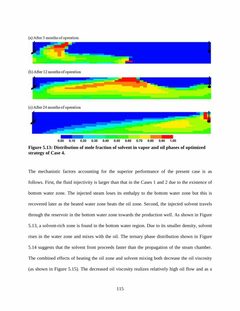
115

Figure 5.13: Distribution of mole fraction of solvent in vapor and oil phases of optimized

strategy of Case 4.

The mechanistic factors accounting for the superior performance of the present case is as

follows. First, the fluid injectivity is larger than that in the Cases 1 and 2 due to the existence of

bottom water zone. The injected steam loses its enthalpy to the bottom water zone but this is

recovered later as the heated water zone heats the oil zone. Second, the injected solvent travels

through the reservoir in the bottom water zone towards the production well. As shown in Figure

5.13, a solvent-rich zone is found in the bottom water region. Due to its smaller density, solvent

rises in the water zone and mixes with the oil. The ternary phase distribution shown in Figure

5.14 suggests that the solvent front proceeds faster than the propagation of the steam chamber.

The combined effects of heating the oil zone and solvent mixing both decrease the oil viscosity

(as shown in Figure 5.15). The decreased oil viscosity realizes relatively high oil flow and as a

116

consequence of short breakthrough time, a shorter operating period. In addition, with a

blowdown strategy, about 99% of solvent can be recovered.

Figure 5.14: Ternary phase distributions of the optimized Case 4.

117

Figure 5.15: Viscosity (cP) distribution of the optimized Case 4 (the grid blocks shown in

white represent region with zero oil saturation).

5.7 Conclusions

In the present work, stochastic optimization was conducted to determine optimum steam and

steam–solvent flooding strategies in thin heavy oil reservoir in cases with and without a bottom

water zone. The key observations are as follows.

The steam injection pressure optimization procedure realized a feasible operating strategy.

However, the achieved cumulative energy injected to produced oil ratio (cEOR) is much

higher than that obtained for SAGD in thicker oil sands reservoirs.

118

The steam–solvent optimization procedure achieved operating strategy with lower cEOR and

WOR than those in the optimized injection pressure-only strategy. The results revealed that a

solvent channel forms at the top of the reservoir after the breakthrough of solvent in the

production well. The formation of the solvent channel promotes oil–solvent mixing as well as

heat transfer to the oil zone which in turn results in better reservoir performance.

The presence of a bottom water zone was found to adversely affect the performance of the

strategy achieved in steam injection pressure-based optimization case. High water-cut due to

water coning leads to relatively high water-to-oil ratio and cEOR. Although the heated

bottom water zone could mobilize oil located above the bottom water in a relatively short

period of time, the overall economics is the worst of all the four investigated optimized cases.

With solvent introduction in the injected fluid, the presence of bottom water was shown to be

a positive factor in promoting oil recovery. The bottom water enhanced mixing of solvent

and oil due to the formation of a solvent-rich zone in the bottom water region. The optimized

strategy in this case achieved the best economic performance. It is well known that the

existence of bottom water worsens cold production and CHOPS performance; however,

based on the results obtained in this study, we propose that solvent-aided steam-flooding

should be considered as a potential operating strategy for thin (<5 m) heavy oil reservoirs,

especially those with bottom water intervals.

119

The net present value calculations suggest, under present economic and reservoir model

assumptions, that solvent co-injection with steam achieves improved economic performance

compared to that of steam-alone operations.

5.8 References







Computer Modeling Group Ltd. (2012). STARS User’s Guide.



Gates, I. D. (2010). Solvent-aided Steam-Assisted Gravity Drainage in Thin Oil Sand Reservoirs.

J Petrol Sci Eng, 74, 138-146.


Calgary.

Metropolis, N., Rosenbluth, A. W., Rosenbluth, M. N., Teller, A. H., & Teller, E. (1953).

Equation of state calculations by fast computing machines. J. Chem. Phys., 21, 1087-

1092.














2012–2021.

Zhao, W., Wang, J., & Gates, I. D. (2012). Thermally-based Operating Strategy and Well

Placement for Thin Heavy Oil Reservoir Paper presented at the The 33rd IEAEOR

Symposium, Regina, Canada.

120

CHAPTER SIX: AN EVALUATION OF ENHANCED OIL RECOVERY STRATEGIES

FOR A HEAVY OIL RESERVOIR AFTER COLD PRODUCTION WITH SAND

This chapter was published in the peer-reviewed journal International Journal of Energy

Research (2014 impact factor 2.42). The citation is as follows: Zhao, W., Wang, J., and Gates,

I.D. An Evaluation of Enhanced Oil Recovery Strategies for a Heavy Oil Reservoir after Cold

Production with Sand. International Journal of Energy Research, DOI: 10.1002/er.3337, 2015.

6.1 Abstract

Cold heavy oil production with sand (CHOPS) is the process of choice for unconsolidated heavy

oil reservoirs with relatively high gas content. The key challenge of CHOPS is that the recovery

factor tends to be between 5% and 15%, implying that the majority of the oil remains in the

ground after the process is rendered uneconomic. Continued cold production (without sands) is

not productive for a post-CHOPS reservoir because of the low oil saturation and depleted

reservoir pressure in the wormhole regions. There is a need to develop viable recovery processes

for post-CHOPS reservoirs. Here, different follow-up processes are examined for a post-CHOPS

heavy oil reservoir. In post-CHOPS cold water flooding, severe water channeling is ineffective at

displacing high viscosity heavy oil. Hot water flooding improves the sweep efficiency and

produces more oil compared with cold water flooding. However, the swept region is limited to

the domain between the neighboring wormhole networks, and the energy efficiency of the

process is relatively poor. Compared with the hot water flooding case, steam flooding achieves

higher oil production rates and lower water use. A cyclic steam stimulation strategy achieves the

best performance regarding oil production rates and water usage. Based on our results, it is

observed that thermally based techniques alone are not capable to recover the oil economically

121

for post-CHOPS reservoirs. However, it is suggested that techniques with combined use of

thermal energy and solvent could potentially yield efficient oil recovery methods for these

reservoirs.

6.2 Introduction

In Western Canada, up to 85% of the heavy oil resources are contained in reservoirs less than 5-

m thick (Adams, 1982) and serve as a very significant portion of energy resources of Canada

(Dincer & Dost, 1996). For heavy oil resources, primary recovery, often referred to as cold

production, recovers between 3% and 15% of the original oil in place with average recovery

factors equal to about 10%. This implies that at the end of the process, when it is rendered

uneconomic, about 90% of the oil remains in the reservoir; thus, given the investment of wells

and infrastructure already in place, there is a substantial incentive to find follow-up recovery

processes that will increase the recovery factor. Secondary and tertiary recovery by water or

polymer flooding could achieve an incremental recovery factor of up to 10% to 15%. However,

these enhanced oil recovery processes tend to be limited to heavy oil reservoirs with oil viscosity

less than about 3000 cP.

By encouraging sand production along with oil recovery, the so-called cold heavy oil production

with sand (CHOPS) technique can recover as much as 15% (Pan et al., 2010). However,

aggressive sand production typically leads to the formation of an extensively connected

wormhole network in the reservoir with zones adjacent to the network depleted of reservoir

pressure. The wormholes and their associated network are believed to be of the order of tens of

centimeters in diameter, extended tens up to a few hundred meters within the reservoir. In many

122

cases, it has been observed that wormholes are connected over long distances (Pan et al., 2010;

Squires, 1993; Yeung, 1995). Squires (1993) reported on fluorescein dye tracer tests in post-

CHOPS field that demonstrated communication between wells with speeds of up to about

400 m/h. Yeung (1995) also documented tracer tests where a fluorescein dye was injected into

one of the production wells of a CHOPS field while the other well continued production. The

tracer tests demonstrated direct communication with the neighboring wells with the dye being

produced with a few hours of injection into wells of up to 500 m away. This also implied that the

dye traveled at a speed of up to several hundred meters per hour. The creation of wormhole

networks and depletion of reservoir driven by the CHOPS process present severe challenges for

applying follow-up processes to recover additional oil after CHOPS operations. It remains

unknown what the optimal recovery process should be for post-CHOPS reservoirs because the

presence of the wormholes in the reservoir is the path of least resistance for injectants. Thus, if a

fluid is injected into the reservoir to mobilize heavy oil, it often bypasses most of the reservoir

because of the extremely high conductivity of the wormholes relative to that of the sand matrix

in between the wormholes.

Because of the complexity and unique features of the post-CHOPS reservoirs, there are

challenges to apply traditional enhanced oil recovery (EOR) methods (Stosur, 1986), and

innovative techniques are being explored. To date, several processes have been examined to

follow CHOPS operation to increase the overall recovery factor from these reservoirs, for

example, hot water flooding (Coskuner and Babadagli, 2013), solvent injection (Chang and

Ivory, 2013; Coskuner et al., 2013; Du et al., 2013; Ivory et al., 2010; Kristoff et al., 2008), in

situ combustion (Chen, 2012), and CO2 flooding (Derakhshanfar et al., 2012; Istchenko, 2012).

123

For post-CHOPS wells, the cyclic solvent injection (CSI) follow-up process has received much

focus and has been tested in field trials (Kristoff et al., 2008). The field trials demonstrated that

the process is feasible. In a previous study, Istchenko and Gates (Istchenko and Gates, 2014)

presented a novel approach to model the evolution of wormholes in heavy oil reservoirs during

CHOPS called the well-wormhole model. Istchenko (Istchenko, 2012) evaluated by detailed

reservoir simulation the CSI follow-up process. Solvents evaluated were mixtures of methane

and propane, and carbon dioxide and propane. His results indicated that CSI was more energy

efficient than thermal method, with a cumulative energy-to-oil ratio (cEOR) between 0.8 and

1.7 GJ/m3 compared with typical values between 7.5 and 10 GJ/m

3 as found in steam-assisted

gravity drainage (SAGD) and cyclic steam stimulation (CSS, also referred to as huff'n'puff). The

results demonstrated that the overall recovery factor could be raised by 68% to 98% over that

achieved by CHOPS.

Here, a well-wormhole network obtained from the operation of four CHOPS wells is used to

evaluate cold and hot water flooding, steam flooding, and CSS as post-CHOPS follow-up

processes to raise the overall recovery factor of the reservoir.

6.3 Reservoir Simulation Model Description

The reservoir model is a three-dimensional model that was derived from a previous CHOPS

study (Istchenko, 2012; Istchenko and Gates, 2014). The model was discretized into a regular

Cartesian grid with dimensions 4 m in both horizontal directions and 1 m in the vertical direction,

resulting in a 200 × 200 × 5 grid, which corresponds to a well pad with dimensions equal to 800

by 800 m with a pay thickness equal to 5 m. Because a post-CHOPS model is used, the

124

wormholes that were evolved during the CHOPS stage of the process are modeled as branched

wells with a diameter equal to 10 cm. For the fluid model, flow of oil, aqueous, and gas phases

were modeled. In the commercial thermal reservoir simulator (Computer Modeling Group Ltd,

2012) used here, the governing equations are given by the convective diffusion equation (with

velocities for the oil, water, and gas phases given by Darcy's law).

and the energy balance:

where all symbols are defined in the nomenclature section. These equations were solved in a

commercial thermal reservoir simulator that uses the finite volume approach. The oil phase

consists of two components – dead heavy oil and solution gas (modeled as methane). The

reservoir simulation model and fluid properties are listed in Table 6.1.

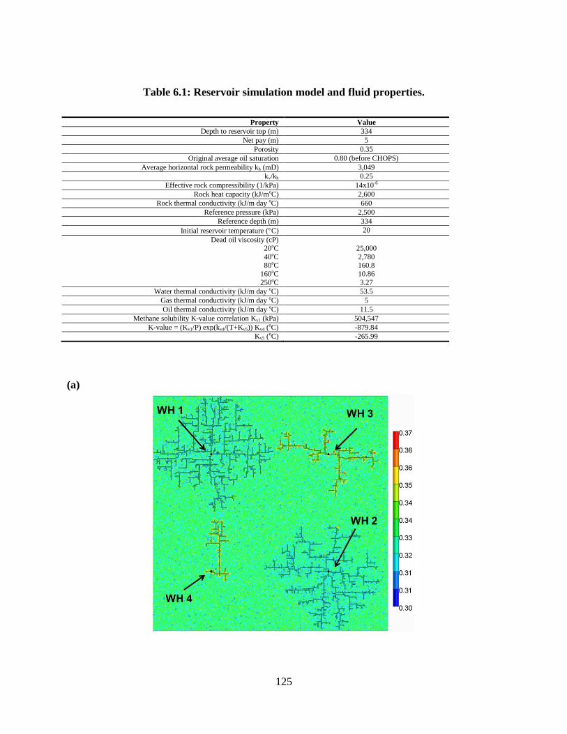
125

Table 6.1: Reservoir simulation model and fluid properties.

Property Value


Net pay (m) 5

Porosity 0.35

Original average oil saturation 0.80 (before CHOPS)

Average horizontal rock permeability kh (mD) 3,049

kv/kh 0.25

Effective rock compressibility (1/kPa) 14x10-6

Rock heat capacity (kJ/moC) 2,600


Reference pressure (kPa) 2,500

Reference depth (m) 334

Initial reservoir temperature (C) 20

Dead oil viscosity (cP)

20oC

40oC 80oC

160oC

250oC

25,000

2,780 160.8

10.86

3.27

Water thermal conductivity (kJ/m day oC) 53.5

Gas thermal conductivity (kJ/m day oC) 5


Methane solubility K-value correlation Kv1 (kPa) 504,547

K-value = (Kv1/P) exp(kv4/(T+Kv5)) Kv4 (oC) -879.84

Kv5 (oC) -265.99

(a)

126

(b)

(c)

Figure 6.1: (a) Porosity, (b) horizontal permeability, in Darcys, and (c) initial oil saturation

profile after the CHOPS operation conducted from four vertical wells, WH1, WH2, WH3,

and WH4. Wormhole network 1 (connected to Well WH1) is located in second grid layer

from bottom of model, wormhole network 2 (connected to Well WH2) is located in third

layer from bottom of model, and wormhole networks 3 and 4 (connected to Wells WH3 and

WH4, respectively) are both located in the fourth layer from the bottom of the model.

127

The original distributions of the porosity, horizontal permeability, and oil saturation of the heavy

oil reservoir are displayed in Figure 6.1. The original oil saturation and reservoir pressure at the

top of the heavy oil column are equal to 0.8 and 2900 kPa, respectively. The four well locations,

WH1, WH2, WH3, and WH4, are also shown. The original oil in place (before CHOPS) is equal

to 8.21 × 105 m

3. The initial condition of the reservoir used in this work is the final result of

CHOPS operation, which was performed over a period of 2 years using the well-wormhole

model as described in Istchenko (Istchenko, 2012). The porosity and permeability distributions,

taken at the elevation to illustrate the wormhole networks that have grown around the CHOPS

wells, are displayed in Figure 6.1. The results show that wormhole networks grow around each

of the four wells during the CHOPS production process. Of the four wells, the wormhole

networks around wells WH1 and WH4 are extensively developed with many branches that

extend up to several meters into the reservoir. On the other hand, the networks associated with

wells WH3 and WH4 are much less developed. The porosity and permeability distributions

reveal the dilation effects of the CHOPS operation in the unconsolidated heavy oil reservoir.

Figures 6.1c and 6.2 display the oil saturation and pressure distributions, respectively, after the

CHOPS operation, at the elevation of the wormhole network, which shows the depletion zone

around the wormhole network. After the CHOPS operation, the oil saturation in the region close

to wormhole networks has dropped to below 0.55 and 0.50 in some regions. From the oil

saturation (Figure 6.1c) and pressure distributions (Figure 6.2), it is observed that the produced

region of WH1 has merged into those of WH3 and WH4. The reservoir pressure of the majority

of unproduced region is still at the original reservoir pressure (2900 kPa), whereas the pressure of

the produced region, especially the regions close to the wormholes, is significantly lower. The

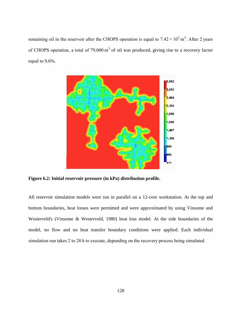
128

remaining oil in the reservoir after the CHOPS operation is equal to 7.42 × 105 m

3. After 2 years

of CHOPS operation, a total of 79,000 m3 of oil was produced, giving rise to a recovery factor

equal to 9.6%.

Figure 6.2: Initial reservoir pressure (in kPa) distribution profile.

All reservoir simulation models were run in parallel on a 12-core workstation. At the top and

bottom boundaries, heat losses were permitted and were approximated by using Vinsome and

Westerveld's (Vinsome & Westerveld, 1980) heat loss model. At the side boundaries of the

model, no flow and no heat transfer boundary conditions were applied. Each individual

simulation run takes 2 to 28 h to execute, depending on the recovery process being simulated.

129

6.4 Follow-up Process Cases

6.4.1 Cold Production (Without Sands)

Foamy oil behavior was intentionally not included in this case to mimic the pressure-depleted

reservoir after CHOPS operation. The four wells with their associated wormhole networks were

open for production with a minimum bottom-hole pressure (BHP) equal to 500 kPa.

6.4.2 Cold Water Flooding

In this case, well WH1 was used as the injector with cold water (20 °C) as injected fluid. Two

cases were investigated with injection pressures equal to 2900 and 5000 kPa, respectively. Wells

WH2, WH3, and WH4 were used as producers subject to 500 kPa BHP. Different well

injector/producer combinations were investigated to understand the impact of the wormholes on

recovery process performance.

6.4.3 Hot Water Flooding

In this case, the injection fluid consisted of hot water at 232 °C injected into well WH1. Two

cases were run with injection pressures equal to 2900 and 5000 kPa, respectively. Different

injection/production well combinations were also explored.

6.4.4 Steam Flooding

In this case, steam is injected with steam quality equal to 0.8 into well WH1. Two cases were

examined with injection pressures equal to 2900 and 5000 kPa, respectively (corresponding to

steam saturation temperatures equal to 232 and 262 °C, respectively). Different

injection/production well combinations were also explored.

130


In this case, a steam huff'n'puff recovery process was used where steam is injected over a period

of time into the wells, after which fluids are produced from the wells for a period of time. The

steam injection and fluid production cycles are repeated. The operating strategy for the CSS

process was devised as follows. During the steam injection period at injection temperature equal

to 232 °C and injection pressure equal to 2900 kPa, the heat loss rate to the overburden over the

first year was found to be equivalent to about 150 m3/day of steam (steam volume expressed as

cold water equivalent (CWE)) and equivalent to 180 and 210 m3/day of steam in the second and

third years of operation, respectively. Ideally, the operating strategy should be designed to direct

the maximum amount of heat to the oil rather than to the overburden. This implies an operating

strategy where the heat is injected rapidly, but before it can conduct a large fraction of it to the

overburden, the heated oil and condensate should be produced from the reservoir. This, in turn,

implies short injection/production cycles. Given these equivalent heat loss steam rates, during the

steam injection period of the wells, the steam injection rate limit was set equal to 150, 180, and

210 m3 CWE/day for the first, second, and third year of operation for any cycles that occurred in

those years, respectively. The maximum steam injection pressure was set equal to 2900 kPa.

After the steam injection period was stopped, each well was converted to production. The

production well was operated with a minimum BHP equal to 500 kPa. After the production

period was completed, the well was converted to steam injection, and a new cycle started.

131


6.5.1 Cold Production (Without Sands)

Over the operating period of 5 years beyond the CHOPS operation, cold production (without

sand) yielded a total of 8.5 m3 produced oil. Essentially, the incremental recovery factor beyond

that of the CHOPS operation is negligible. This very low production volume is because after

CHOPS, the reservoir in the neighborhood of the wormhole networks is depressurized and

depleted of solution gas (and thus no foamy oil flow). The methane mole fraction in the oil phase

in the produced region after CHOPS has dropped to 0.02–0.05 from an original value equal to

0.11 at original conditions (before the CHOPS operation). This suggests both a poor solution gas

drive and a high live oil viscosity. Thus, there is little drive and relatively low oil mobility and

therefore nearly no incremental oil.

6.5.2 Cold Water Flooding

With well WH1 as the single injector at an injection pressure equal to 2900 kPa, the total injected

water volume reached 70,582 m3 with total oil production equal to 612 m

3 over an operating

period of 5 years. This corresponds to an incremental recovery factor equal to 0.07% over that of

the CHOPS operation. After only 46 days, the results reveal that the water-cut has risen to 90%.

Over the 5-year operation life, the cumulative water-cut was equal to 99.1%. Analysis of the

water flow within the reservoir reveals that the injected water breaks through to the neighboring

wormhole network. After the CHOPS operation, the smallest tip-to-tip distance between the

wormhole networks centered on wells WH1 and WH4 is equal to about 28 m, whereas between

the networks surrounding wells WH1 and WH3, it is equal to about 17 m. The large pressure

gradient and the high initial water saturation (Li & Li, 2014) in the separating region between the

132

networks led to rapid water break through, as shown in Figure 6.3. The local nature of these

regions, compounded with the poor mobility ratio, results in a very small swept region and

therefore small oil production.

Figure 6.3: Oil saturation profile of the water flooding strategy (with WH1 as injector and

WH2-4 as producers) after 5 years. The two regions circled are those where water break

through from one network to the other.

With an increase of the injection pressure from 2900 to 5000 kPa, the cumulative oil production

volume after 5 years of operation was found to be equal to 1394 m3, giving an incremental

recovery factor equal to 0.17% over that of the CHOPS operation. At the end of the process, the

cumulative water-cut is equal to 99.0%. As with the lower injection pressure, water break

133

through occurred in the locations where the networks were closest. Other injector/producer

combinations revealed similar results.

6.5.3 Case 3: Hot Water Flooding

As with cold water flooding, water break through for the hot water flooding case also took place

relatively quickly. After 30 days of hot water injection, the water-cut exceeded 90%. Figure 6.4

displays the oil saturation distribution for the hot water flooding case with well WH1 as the

single injector and wells WH2–4 as producers after 5 years of operation. The results demonstrate

that water break occurred within the regions between the tips of the networks dominantly

between wells WH1 and WH3 and between wells WH1 and WH4. Because of the improved

mobility ratio that occurs in hot water flooding (due to reduced oil viscosity on heating), the

swept regions are larger than those observed in the (cold) water flooding case. Figure 6.5 shows

the cumulative oil production and the cumulative hot water injected-to-oil produced ratio. Within

a period of 5 years, a total of about 14,580 m3 of oil is produced, which is 24 times that of the

water flooding case. The oil production rate is relatively stable over the production period and

could be continued for several years more. However, the amount of hot water injected is also

quite substantial; for each cubic meter of oil produced, about 107 m3 of hot water (at 232 °C) is

injected. To characterize the energy requirements, we calculated the cumulative energy injected

(as hot water enthalpy)-to-oil ratio (cEOR). For hot water flooding at 2900 kPa injection

pressure, the cEOR is found to be equal to about 99.6 GJ/m3 (a detailed comparison of the energy

requirements for all the investigated cases is listed in Table 2). Considering the energy content of

oil to be 37 GJ/m3, one can see that the hot water flooding consumes more energy than is

produced in the form of chemical energy.

134

Figure 6.4: Oil saturation profile of the hot water flooding strategy (with an injection

pressure of 2900 kPa) after 5 years. The two regions circled are those where water break

through.

Figure 6.5: Cumulative oil production and hot water-to-oil ratio of the hot water flooding

(use WH1 as injector and WH2-4 as producers).

135

Although hot water flooding is not an efficient EOR method by itself alone, it is suggested based

on experimental results that it can be used in combination with other techniques such as solvent

injection to enable more effective oil recovery (Coskuner et al., 2013).

6.5.4 Steam Flooding

In the steam flooding base case, we first investigated steam break through by using well WH1 as

steam injector. Figure 6.6 shows oil saturation and temperature profile after 1 year of operation.

The results reveal that steam mainly breaks through into the network of well WH3 after 1 year of

operation. Compared with hot water flooding, steam flooding realized more oil production equal

to 25,643 m3 over the 5-year operation with a cumulative steam-to-oil ratio (cSOR; steam

expressed as CWE) equal to 44 m3/m

3, as shown in Figure 6.7. The water usage is improved

compared with the hot water flooding case. However, the cEOR is equal to about 107.3 GJ/m3,

which is 8% larger than that of hot water flooding. This is because of the additional heat invested

in the steam in the form of latent heat.

136


reservoir after 1 year of steam flooding with WH1 as injector and WH2-4 as producers.

Figure 6.7: Cumulative oil production and steam oil ratio of the steam flooding (use WH1

as injector and WH2-4 as producers).

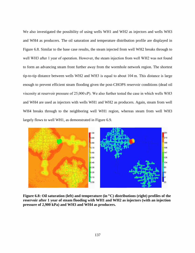
137

We also investigated the possibility of using wells WH1 and WH2 as injectors and wells WH3

and WH4 as producers. The oil saturation and temperature distribution profile are displayed in

Figure 6.8. Similar to the base case results, the steam injected from well WH2 breaks through to

well WH3 after 1 year of operation. However, the steam injection from well WH2 was not found

to form an advancing steam front further away from the wormhole network region. The shortest

tip-to-tip distance between wells WH2 and WH3 is equal to about 104 m. This distance is large

enough to prevent efficient steam flooding given the post-CHOPS reservoir conditions (dead oil

viscosity at reservoir pressure of 25,000 cP). We also further tested the case in which wells WH3

and WH4 are used as injectors with wells WH1 and WH2 as producers. Again, steam from well

WH4 breaks through to the neighboring well WH1 region, whereas steam from well WH3

largely flows to well WH1, as demonstrated in Figure 6.9.


reservoir after 1 year of steam flooding with WH1 and WH2 as injectors (with an injection

pressure of 2,900 kPa) and WH3 and WH4 as producers.

138


reservoir after 1 year of steam flooding with WH3 and WH4 as injectors (with an injection

pressure of 2,900 kPa) and WH1 and WH2 as producers.

The main observation derived from the steam flooding cases is relatively quick steam break

through between the shortest tip-to-tip distances between the wormhole networks. If the tip-to-tip

distance is too large, in the case shown here, equal to about 100 m, the steam front is not

effective at displacing oil between the wormhole networks.


Figure 6.10 displays the oil production rate and cumulative oil production from the CSS

operating strategy over a period of 4 years of operation. Compared with a typical CSS operation

in Cold Lake, Alberta, the CSS operation of the present post-CHOPS reservoir exhibits much

shorter operating periods in terms of both injection and production. A key difference between

Cold Lake CSS and the post-CHOPS operation is that steam fracturing is used in Cold Lake to

inject the targeted amount of steam injection to achieve effective steam conformance around the

139

CSS well, fracture the formation to enhance the permeability in the near-well region, dilate the

system so that formation recompaction aids production, and to break up shale layers that sit

within the oil column. Here, because the wormhole network acts as a conduit to achieve steam

conformance within the reservoir, the steam can be injected under the fracture pressure. In the

CSS operation evaluated here, the injection period of the first two cycles are 36 and 31 days

long, respectively, during which the reservoir is pressurized up and volume previously occupied

by gas is filled up with steam. After the steam is injected, the steam condenses and releases its

latent heat to the surrounding formation. The injection periods of the third to ninth cycles are

typically between 10 and 14 days, whereas cycles 10 and beyond become longer. In most cycles,

the production period ranges from 10% to 30% longer than the injection periods.

Figure 6.10: Oil production rate and cumulative oil production of the CSS process.

140

Within a period of 4 years, a total of 25 cycles are completed with the final production period of

the last cycle being equivalent to a wind-down period. As shown in Figure 6.10, the cyclic peak

oil rates are found to range from 170 to 390 m3/day. Over the 4-year operation life, the calendar

day oil rate (average over the entire period of the operation) is equal to about 69 m3/day, leading

to a cumulative oil production equal to 100,230 m3.

Figure 6.11 shows the oil saturation, temperature, and pressure distributions at the ends of cycles

1, 5, 10, and 22. It can be observed that the oil in the neighborhood of the wormholes is depleted

with greater conformance within the network as the cycle number increases. This is because of

the cyclic manner of the process where after the steam injection period, the oil in the

neighborhood of the network is heated, resulting in its thermal expansion and lower viscosity,

which then is depleted by the network during the production period. Because of the increase of

water saturation within the oil-depleted zone, more steam can be injected into the reservoir in

each subsequent cycle, which in turn improves steam conformance and oil production. After

steam injection, the temperature is equal to roughly that of the injected steam (232 °C). After the

production period is completed, the temperature drops, as shown in Figure 11, to values equal to

about 140 °C. The pressure distribution at the end of each cycle demonstrates that the pressure

depletion zone grows after each cycle.

141

Figure 6.11: Oil saturation, temperature, and pressure distributions at the end of Cycles 1,

5, 10, and 22.

Figure 6.12 shows the cumulative cSOR of the CSS process versus time. It can be seen that the

increase in injectivity and subsequent oil production over the first 2 years leads to a relatively

rapid decline of the cSOR. As the process matures, the cSOR achieves a roughly constant value

just higher than 10 m3/m

3. However, as the heated zone grows larger, the heat loss to the

EndofCycle1

OilSatura on Temperature,deg.C Pressure,kPa

EndofCycle5

EndofCycle10

EndofCycle22

Pressure(kPa)

OilSatura on

Temp.,deg.C

142

overburden also increases. At the same time, the oil gradually becomes depleted, and as a

consequence, the cSOR grows slowly with time. At the end of 4 years, the cSOR is equal to

11.2 m3/m

3, which corresponds to a cEOR equal to 26.5 GJ/m

3 (Table 6.2).

Table 6.2: Comparison of average oil production rates, cumulative energy injected-to-oil

ratio (cEOR), cumulative injected water-to-oil ratio (cWOR), and CO2 emission for the

investigated cases over a period of 5 years; CSS case was run for 4 years total operating

life. For the cSOR, the steam volume is reported as cold water equivalent. The recovery

after the initial CHOPS operation is equal to 9.6%.

Cases Average oil

production

rate (m3/day)

cEOR

(GJ/m3)

cWOR

(m3/m

3)

CO2

emissions/oil

production

(kg/m3)

Incremental Recovery

Factor beyond

primary CHOPS

operation (%)

Cold production 0 - - - 0

Water flooding 0.3 - 115.3 - 0

Hot water flooding 8.0 99.6 106.6 8,267 1.8

Steam flooding 14.0 107.3 44.9 8,906 3.1

CSS 68.6* 26.5 11.2 2,200 12.2

* Calendar day oil rate (average oil rate throughout entire CSS operating life)

143

Figure 6.12: Cumulative steam-to-oil ratio in the cyclic steam stimulation process.

We further analyzed the different components of heat loss during the CSS process (Figure 6.13).

It was found that the heat losses to overburden and underburden, due to the relatively small

reservoir thickness, quickly rise to about 40% of the total injected heat after 4 months of

operation and remain relatively constant at about 43% for the last 2.5 years. The heat in the

produced fluids increases at a slower pace than that of heat loss. At the end of 4 years of

operation, the produced heat rises to 54% of the total injected heat. This indicates that the energy

efficiency of the present CSS can be further improved if the produced heat can be utilized more

efficiently in the process, such as in some water/steam preheating stages.

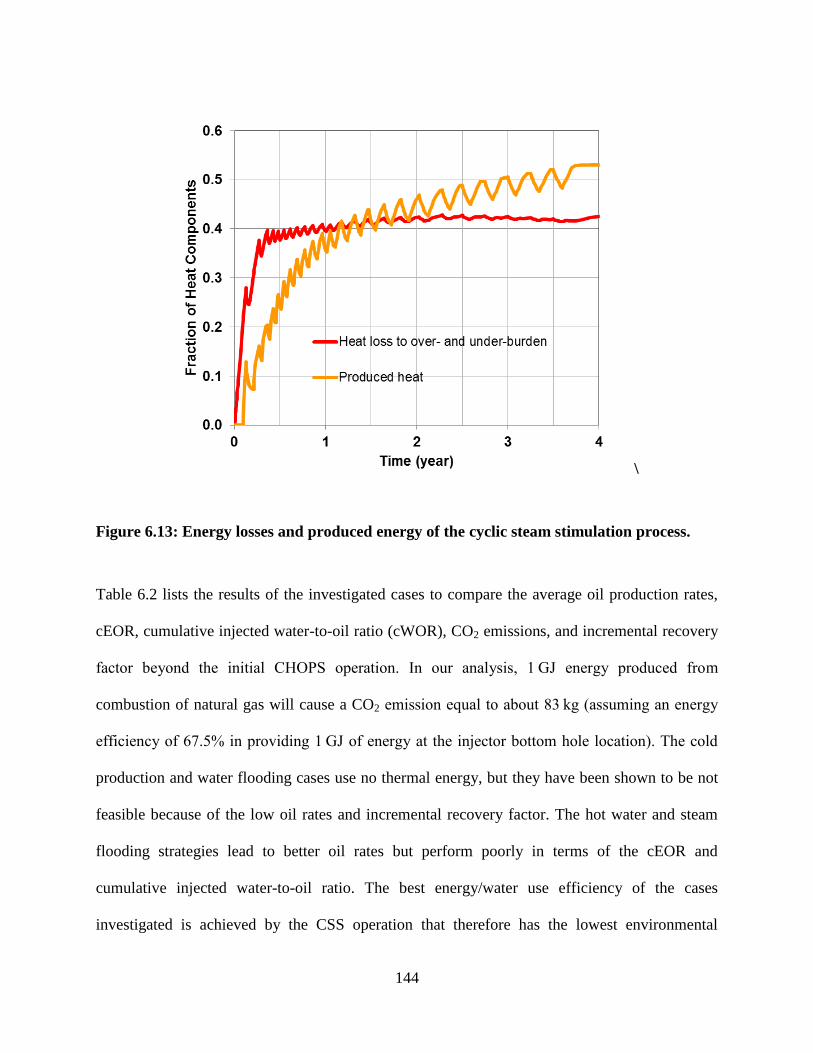
144

\

Figure 6.13: Energy losses and produced energy of the cyclic steam stimulation process.

Table 6.2 lists the results of the investigated cases to compare the average oil production rates,

cEOR, cumulative injected water-to-oil ratio (cWOR), CO2 emissions, and incremental recovery

factor beyond the initial CHOPS operation. In our analysis, 1 GJ energy produced from

combustion of natural gas will cause a CO2 emission equal to about 83 kg (assuming an energy

efficiency of 67.5% in providing 1 GJ of energy at the injector bottom hole location). The cold

production and water flooding cases use no thermal energy, but they have been shown to be not

feasible because of the low oil rates and incremental recovery factor. The hot water and steam

flooding strategies lead to better oil rates but perform poorly in terms of the cEOR and

cumulative injected water-to-oil ratio. The best energy/water use efficiency of the cases

investigated is achieved by the CSS operation that therefore has the lowest environmental

145

footprint as measured by the CO2 emission. It also achieved the highest oil production rates.

However, considering a typical commercial SAGD operation with a cEOR equal to 10 GJ/m3, the

current CSS follow-up process for the post-CHOPS reservoir perform poorly regarding its

26.5 GJ/m3 cEOR.

6.6 Conclusions

In the present work, reservoir simulation was used to evaluate five different operating strategies

as follow-up recovery process candidates for a post-CHOPS reservoir. The following

observations are found based on the detailed analysis.

Cold production (without sands) is not productive for a post-CHOPS reservoir because of the

low oil saturation and depleted reservoir pressure in the wormhole regions.

Water channeling and high oil viscosity (coupled with depleted solution gas in the post-

CHOPS reservoir) lead to infeasibility of a (cold) water flooding strategy. In this strategy,

water quickly breaks through from the tip-to-tip regions of the neighboring wormhole

networks, which leads to extremely poor sweep efficiency.

Hot water flooding improved the sweep efficiency and produces much more oil compared

with (cold) water flooding. However, the swept region is limited to the domain close to the

shortest tip-to-tip of the neighboring wormhole networks.

Steam flooding achieved higher oil production rates and lower water use compared with hot

water flooding but still uses a large amount of energy comparable to that of the hot water

flooding strategy. It is found that steam break through occurs only in the region directly

between the wormhole networks.

146

The CSS strategy achieved the best performance regarding oil production rates, water usage,

and CO2 emissions. The injection periods are shorter than a typical CSS operation because of

existing wormhole networks, which provide good injectivity permitting reasonable steam

conformance around the injection wells. However, the energy cost per unit volume of oil

produced is still much higher than that of SAGD operations in oil sands reservoirs. In

summary, we suggest that CSS is the most efficient thermal recovery technique for these

reservoirs.

6.7 References



Chang, J., & Ivory, J. (2013). Field-scale Simulation of Cyclic Solvent Injection (CSI). Journal

of Canadian Petroleum Technology, 52, 251-265.



Alberta, Canada.


Coskuner, G., K, K. N., & Babadagli, T. (2013). An enhanced oil recovery technology as a

follow up to cold heavy oil production with sand. presented at. Paper presented at the

The SPE Heavy Oil Conference Canada, Calgary, Alberta.




Dincer, I., & Dost, S. (1996). On the energy resources of Canada. International Journal of

Energy Research, 20, 595-607.

Du, Z., Zeng, F., & Chan, C. (2013). An experimental study of the post-CHOPS cyclic solvent

injection process. Paper presented at the The SPE Heavy Oil Conference Canada,

Calgary, Alberta.


Calgary.





147

Kristoff, B. J., KD, K. D. K., Preston, C. K., Worth, K., & Sawatzky, R. (2008). Joint

implementation of vapour extraction – heavy oil recovery process. Paper presented at the

The World Heavy Oil Congress, Edmonton, Alberta.

Li, K., & Li, Y. (2014). Effect of initial water saturation on crude oil recovery and water cut in

water-wet reservoirs. International Journal of Energy Research, 38, 1599-1607.






Canada.

Stosur, J. J. G. (1986). The potential of enhanced oil recovery. International Journal of Energy

Research, 10, 357-370.







148

CHAPTER SEVEN: CONCLUSIONS AND RECOMMENDATIONS

7.1 Summary and Conclusions

The research work presented in this thesis describes the investigations of different recovery

methods for thin heavy oil reservoirs. The conclusions are summarized in the following sections.

7.1.1 Unexploited Thin Heavy Oil Reservoirs

Cold production (without sand) is not effective to thin heavy oil reservoirs with high oil

viscosities, indicated by the very low recovery factors.

SAGD strategies are not applicable due to very low heat utilization efficiency caused by

excessive heat loss to over- and under-burden and hot water production.

With optimization of injecting pressure, steam-flooding strategy achieved higher heat

utilization efficiency compared to SAGD. However it is still economically expensive because

of its high energy injected to oil ratio (EOR).

Hot water flooding is more effective compared with steam flooding with respect to EOR. The

oil rate resulted from the pressure gradient rather than oil viscosity reduction due to the

injected heat. The use of hot water led to a lower average reservoir temperature and therefore

reduced heat loss to the over- and under-burden. With optimization in pressure and

temperature, the performance of hot water flooding strategy can be further improved.

The steam–solvent optimization procedure achieved operating strategy with lower cEOR and

water to oil ratio (WOR) than those in the optimized steam-flooding strategy. The presence

of bottom water was shown to be a positive factor in promoting oil recovery.

149

7.1.2 Post-CHOPS Reservoirs

Cold production (without sands) is not productive for a post-CHOPS reservoir because of the

low oil saturation and depleted reservoir pressure in the wormhole regions.

Water channeling and high oil viscosity (coupled with depleted solution gas in the post-

CHOPS reservoir) lead to infeasibility of a (cold) water flooding strategy.

Hot water flooding improved the sweep efficiency and produces much more oil compared

with (cold) water flooding. However, the swept region is limited to the domain close to the

shortest tip-to-tip of the neighboring wormhole networks.

Steam flooding achieved higher oil production rates and lower water use compared with hot

water flooding but still uses a large amount of energy comparable to that of the hot water

flooding strategy. It is found that steam break through occurs only in the region directly

between the wormhole networks.

The CSS strategy achieved the best performance regarding oil production rates, water usage,

and CO2 emissions. The injection periods are shorter than a typical CSS operation because of

existing wormhole networks, which provide good injectivity permitting reasonable steam

conformance around the injection wells. It is suggested that that CSS is the most efficient

thermal recovery technique for these reservoirs.

7.2 Recommendations for Future Study

Based on research results included in the thesis, the following recommendations are suggested

for future study:

1. In the present study, the dead oil viscosity used in reservoir model is carefully chosen to be

150

15,000 cP to investigate the effectiveness of different recovery strategies for reservoirs with

this high oil viscosity. It is recommended to further investigate the oil viscosity variations on

the efficiency of the proposed strategies.

2. In the post-CHOPS work, we have studied a number of thermally based enhanced oil

recovery methods. It is recommended that further work on investigating recovery processes

combining use of thermal energy with different compositions of solvents involved. .

3. Hot water flooding process with optimized injecting pressure has been proposed as an

effective strategy. It is recommended to compare this strategy with possible field test for

further verification.

4. Solvent-aided steam flooding processes are shown by reservoir simulation to be effective

strategies, especially for reservoir with bottom water. It is therefore worth-doing to validate

this strategy with field test if available in the future.

151

References



Akbarzadeh, K., Hammami, A., Kharrat, A., Zhan, D., Allenso, S., Creek, J. L., . . . Solbakken,

T. (2007). Asphaltenes—problematic but rich in potential. Oilfield Rev, 19(2), 22-43.

Allen, J. C. (1978). Canada Patent No. 1027851.





Boberg, T.C. and Lantz, R.B. (1966). Calculation of the Production Rate of a Thermally

Stimulated Well. Journal of Petroleum Technology, 18, 1613–1623.

Butler, R., & Mokrys, I. (1991). A New Process (VAPEX) For Recovering Heavy Oils Using

Hot Water And Hydrocarbon Vapour. Journal of Canadian Petroleum Technology,

30(1), 97-106.

Butler, R. M. (1985). A New Approach To The Modelling Of Steam-Assisted Gravity Drainage.


Butler, R. M. (1997). United States Patent No. 5,607,016.

Canadian Association of Petroleum Producers. (2015). Crude Oil: Forcast, Markets &

Transportation.

Canadian Natural Resources Ltd. (2011). Canadian Natural Resources Ltd, 2010 Annual Report

Retrieved from http://www.cnrl.com/upload/media_element/385/01/cn_2010ar.pdf

Chang, J., Ivory, J., & Beaulieu, G. (2014). Pressure Maintenance at post-CHOPS Cyclic

Solvent Injection (CSI) Well Using Gas Injection at Offset Well. Paper presented at the

The SPE Heavy Oil Conference-Canada, Calgary, Alberta.



Alberta, Canada.

Christensen, J. R., Stenby, E. H., & Skauge, A. (2001). Review of WAG Field Experience. SPE

Reservoir Evaluation & Engineering, 4(2), 97-106.

http://www.cnrl.com/upload/media_element/385/01/cn_2010ar.pdf

152


Crowfoot, C. (2012). Alberta’s Energy Reserves 2011 and Supply/Demand Outlook 2012–2021.




Diaz-Munoz, J., & Farouq Ali, S. M. (1975). Simulation of Cyclic Hot Water Stimuation of

Heavy Oil Wells.

Dong, L. (2012). Effect of vapor-liquid phase behavior of steam-light hydrocarbon systems on

steam assisted gravity drainage process for bitumen recovery Fuel, 95, 159-168.

Dong, M., Ma, S., & Liu, Q. (2009). Enhanced heavy oil recovery through interfacial instability:

a study of chemical flooding for Brintnell heavy oil. Fuel, 88, 1049-1056.

Dong, M., Huang, S.-S., & Hutchence, K. (2006). Methane Pressure-Cycling Process With

Horizontal Wells for Thin Heavy-Oil Reservoirs. SPE Reservoir Evaluation &


Dusseault, M. B., & El-Sayed, S. (2000). Heavy-Oil Production Enhancement by Encouraging

Sand Production. Paper presented at the The 2000 SPE/DOE Improved Oil Recovery

Symposium Tulsa, Oklahoma.

Edgar, A., Fernandez, R., & Bashbush, J. L. (2008). Horizontal Alternate Steam Drive Process

for the Orinoco Heavy Oil Belt in Eastern Venezuela. Paper presented at the International

Thermal Operations and Heavy Oil Symposium, Calgary, Alberta, Canada.

Farouq Ali, S. M. (1974). Heavy Oil Recovery – Principles, Practicality, Potential, and

Problems. Paper presented at the The Rocky Mountain Regional Meeting, Billings,

Montana, USA.




Gates, I. D. (2010). Solvent-aided Steam-Assisted Gravity Drainage in thin oil sand reservoirs.

Journal of Petroleum Science and Engineering, 74, 138-146.

Gates, I. D., & Leskiw, C. (2008). Impact of Steam Trap Control on Performance of Steam-

Assisted Gravity Drainage Paper presented at the The Canadian International Petroleum

153

Conference/SPE Gas Technology Symposium 2008 Joint Conference (the Petroleum

Society’s 59th Annual Technical Meeting), Calgary, Alberta, Canada.

Gates, I. D., & Chakrabarty, N. (2008). Design of the steam and Solvent Injection Strategy in

Expanding Solvent Steam-Assisted Gravity Drainage. J Can Petrol Technol, 47, 12-20.



Gates, I. D., Kenny, J., Hernandez-Hdez, I. L., & Bunio, G. L. (2007). Steam Injection Strategy

and Energetics of Steam-Assisted Gravity Drainage. SPE Reserv Eval Eng, 10, 19-34.

Geilikman, M.B., Dusseault, M.B. and Dullien, F.A.: “Fluid Production Enhancement by

Exploiting Sand Production,” presented at SPE/DOE Improved Oil Recovery

Symposium, Tulsa, Oklahoma, SPE 27797, 17-20 April, 1994.




Calgary.



Jamaloei, B. Y., Kharrat, R., & Asghari, K. (2012). The influence of salinity on the viscous

instability in viscous-modified low-interfacial tension flow during surfactant-polymer

flooding in heavy oil reservoir. Fuel, 97, 174-185.

Krumrine, P. H., Lefenfeld, M., & Romney, G. A. (2014). Investigation of Post CHOPS

Enhanced Oil Recovery of Alkali Metal Silicide Technology. Paper presented at the The

SPE Heavy Oil Conference-Canada, Calgary, Alberta, Canada.

Kulkarni, M. M., & Rao, D. N. (2005). Experimental investigation of miscible and immiscible

Water-Alternating-Gas (WAG) process performance. Journal of Petroleum Science and


Larter, S., Adams, J., Gates, I. D., Bennett, B., & Huang, H. (2008). The Origin, Prediction and

Impact of Oil Viscosity Heterogeneity on the Production Characteristics of Tar Sands and

Heavy Oil Reservoirs. Journal of Canadian Petroleum Technology, 47, 52-61.

Martin, W. L., Dew, J. N., Powers, M. L., & Steves, H. B. (1967). Results of a Teriary Hot

Waterflood in a Thin Sand Reservoir. J Can Petrol Technol, 243, 739-750.

154

Metropolis, N., Rosenbluth, A. W., Rosenbluth, M. N., Teller, A. H., & Teller, E. (1953).

Equation of state calculations by fast computing machines. J. Chem. Phys., 21, 1087-

1092.

Meyer, R. F., Attanasi, E. D., & Freeman, P. A. (2007). Heavy Oil and Natural Bitumen

Resources in Geological Basins of the World




National Energy Board. (2015). Estimated Production of Canadian Crude Oil and Equivalent

Retrieved from https://www.neb-one.gc.ca/nrg/sttstc/crdlndptrlmprdct/stt/stmtdprdctn-eng.html.

Nasr, T. and Isaacs, E. (2001). Process For Enhancing Hydrocarbon Mobility Using a Steam

Additive, U.S. Patent 6230814.

Nezhad, S., Mojarad, M., Paitakhti, S., Moghadas, J., & Farahmand, D. (2006). Experimental

Study on Applicability of Water.Alternating-CO2 injection in the Secondary and Tertiary

Recovery. Paper presented at the The First International Oil Conference and Exhibition in

Mexico, Cancun, Mexico.






London.

Reddy, J. N. (2005). An Introduction to the Finite Element Method (3rd Ed.): McGraw-Hill.



700-714.






700-714.

https://www.neb-one.gc.ca/nrg/sttstc/crdlndptrlmprdct/stt/stmtdprdctn-eng.html

155

Shu, W. R. (1984). A viscosity correlation for mixtures of heavy oil, bitumen, and petroleum

fractions. Soc. Pet. Eng. J., 24(3), 277-282.



Canada.



Stone, E. J., Lowe, J. A., & Shine, K. P. (2009). Thee impact of carbon capture and storage on

climate. Energy Environ. Sci., 2, 81-91.






2012–2021.







Yuan, J.-Y., Tremblay, B., & Babchin, A. (1999). A Wormhole Network Model of Cold

Production in Heavy Oil. Paper presented at the The 1999 SPE International Thermal

Operations and Heavy Oil Symposium, Bakersfield, California.

Zhao, W., Wang, J., & Gates, I. D. (2014). Thermal recovery strategies for thin heavy oil

reservoirs Fuel, 117, 431-441.

Zhao, W., Wang, J., & Gates, I. D. (2012). Thermally-based Operating Strategy and Well

Placement for Thin Heavy Oil Reservoir Paper presented at the The 33rd IEAEOR

Symposium, Regina, Canada.

oil recovery strategies for thin heavy oil reservoirs

Documents