DI

SC

US

SI

ON

P

AP

ER

S

ER

IE

S

Forschungsinstitut zur Zukunft der ArbeitInstitute for the Study of Labor

Oil Exports and the Iranian Economy

IZA DP No. 4537

October 2009

Hadi Salehi EsfahaniKamiar MohaddesM. Hashem Pesaran

Oil Exports and the Iranian Economy

Hadi Salehi Esfahani University of Illinois at Urbana-Champaign

Kamiar Mohaddes

University of Cambridge

M. Hashem Pesaran University of Cambridge,

University of Southern California and IZA

Discussion Paper No. 4537 October 2009

IZA

P.O. Box 7240 53072 Bonn

Germany

Phone: +49-228-3894-0 Fax: +49-228-3894-180

E-mail: iza@iza.org

Any opinions expressed here are those of the author(s) and not those of IZA. Research published in this series may include views on policy, but the institute itself takes no institutional policy positions. The Institute for the Study of Labor (IZA) in Bonn is a local and virtual international research center and a place of communication between science, politics and business. IZA is an independent nonprofit organization supported by Deutsche Post Foundation. The center is associated with the University of Bonn and offers a stimulating research environment through its international network, workshops and conferences, data service, project support, research visits and doctoral program. IZA engages in (i) original and internationally competitive research in all fields of labor economics, (ii) development of policy concepts, and (iii) dissemination of research results and concepts to the interested public. IZA Discussion Papers often represent preliminary work and are circulated to encourage discussion. Citation of such a paper should account for its provisional character. A revised version may be available directly from the author.

IZA Discussion Paper No. 4537 October 2009

ABSTRACT

Oil Exports and the Iranian Economy This paper develops a long run growth model for a major oil exporting economy and derives conditions under which oil revenues are likely to have a lasting impact. This approach contrasts with the standard literature on the “Dutch disease” and the “resource curse”, which primarily focus on short run implications of a temporary resource discovery. Under certain regularity conditions and assuming a Cobb Douglas production function, it is shown that (log) oil exports enter the long run output equation with a coefficient equal to the share of capital. The long run theory is tested using a new quarterly data set on the Iranian economy over the period 1979Q1-2006Q4. Building an error correction specification in real output, real money balances, inflation, real exchange rate, oil exports, and foreign real output, the paper finds clear evidence for two long run relations: an output equation as predicted by the theory and a standard real money demand equation with inflation acting as a proxy for the (missing) market interest rate. Real output in the long run is shaped by oil exports through their impact on capital accumulation, and the foreign output as the main channel of technological transfer. The results also show a significant negative long run association between inflation and real GDP, which is suggestive of economic inefficiencies. Once the effects of oil exports are taken into account, the estimates support output growth convergence between Iran and the rest of the world. We also find that the Iranian economy adjusts quite quickly to the shocks in foreign output and oil exports, which could be partly due to the relatively underdeveloped nature of Iran’s financial markets. JEL Classification: C32, C53, E17, F43, F47, Q32 Keywords: growth models, long run relations, Iranian economy, oil price,

foreign output shocks, error correcting relations Corresponding author: M. Hashem Pesaran Faculty of Economics University of Cambridge Sidgwick Avenue Cambridge, CB3 9DD United Kingdom E-mail: mhp1@econ.cam.ac.uk

1 Introduction

In this paper we develop a long run output relation for a major oil exporting economywhere oil income to output ratio is expected to remain high over a prolonged period. Thisapproach contrasts with the �Dutch disease�and �resource curse� literature that considersthe revenues from the resource to be intrinsically temporary and focusses on the relativelyshort term implications of the resource discovery. See Corden and Neary (1982), Krugman(1987), Neary and van Wijnbergen (1986), and van der Ploeg and Venables (2009) for arecent survey. We extend the stochastic growth model developed in Binder and Pesaran(1999) to allow for the possibility that a certain fraction of oil export revenues is invested inthe domestic economy. We distinguish between the two cases where the growth of oil income,g0, is less than the natural growth rate (the sum of the population growth, n, and the growthof technical progress) and when g0 � g + n. Under the former, the e¤ects of oil income onthe economy�s steady growth rate will vanish eventually, whilst under the latter, oil incomeenters the long run output equation with a coe¢ cient which is equal to the share of capitalif it is further assumed that the underlying production technology can be represented as aCobb-Douglas production function.The empirical validity of the long run output equation for the Iranian economy is exam-

ined by incorporating it into a vector autoregressive error correction model augmented withforeign output. The resultant VARX* model is estimated using quarterly observations overthe period 1979Q1-2006Q4. The domestic variables included in the model are real GDP, therate of in�ation based on consumer price index (CPI), the o¢ cial and �free�market exchangerates, and money and quasi money. Unlike most other macro models, ours does not includethe interest rate as an explicit variable because the domestic credit markets in Iran operateunder tight controls and the interest rate is not market-determined. But assuming that theFisher equation holds in the long run, the in�ation rate can be used as a proxy for theinterest rate. The foreign output variable is constructed as a weighted average of the logoutput of Iran�s trading partners with the weights based on the relative size of their tradewith Iran (exports plus imports).A number of models of Iran�s macroeconomy have been developed in the past. The

distinctive features of our model are: (1) a theory derived long run model for oil exportingcountries in which the long run role of oil export revenues for growth is explicitly modeled;(2) a careful and parsimonious modeling of the ways in which major external variablesenter into the macroeconomic equations in Iran, taking into account the variety of channelsthrough which the variables in�uence each other, including the implicit response of thegovernment to macroeconomic developments; (3) parameterization of the model to allow forthe measurement and testing of the macro-level impact of oil exports and global technologicalprogress on the Iranian economy; (4) joint modeling and estimation of output, in�ation,money supply, and the real exchange rate, in contrast to models that focus on output orin�ation alone, while treating the other variables as exogenous; and (5) use of quarterly data.The maximum likelihood estimates of the VARX* model support the existence of two long

run relations, namely the real output and the real money demand equations, as predictedby the theory. Furthermore, it is not possible to reject the hypothesis that real output,real money balances, real oil income, and foreign output are co-trending. The evidence alsosupports the existence of a long run relation between domestic output, foreign output, and

2

real oil exports, although we also �nd that in�ation has a statistically signi�cant negativee¤ect on real output. Once the e¤ects of oil exports are taken into account, the estimatessupport output growth convergence between Iran and the rest of the world. These resultsseem to be reasonably robust regardless of how foreign output is constructed, what measureof the exchange rate is used, and whether a dummy variable for revolution and war (overthe period 1979Q1-1988Q2) is included in the model.From the estimates, several conclusions can be drawn. One key result is the economy�s

fast adjustment to shocks, when compared to the response rates of other economies, especiallythe developed ones. This seems to be due to the limitations of Iran�s �nancial markets thatrestrict expenditure smoothing options and thereby cause the economy to move up and downquickly as external and internal conditions change. Second, we �nd that although Iran maylag behind its main trading partners in terms of technology levels, it has experienced asimilar rate of technological progress over the past three decades. Third, in the long run,oil exports contribute to real income through real capital accumulation. As a result, theelasticity of the aggregate real income with respect to real oil revenues (measured in term ofdomestic output units) is equal to the marginal product of capital. We con�rm this resultby showing that the nominal dollar value of oil revenues has the same impact on the realGDP as would be caused by a decline in the dollar value of one unit of domestic output.Fourth, our estimates suggest that in Iran, the output elasticity of capital (or the share ofcapital) is about 0.26. This estimate is lower than the one often used in studies of Iran�seconomy. But, it seems quite reasonable given the large resource rents that can be channeledtowards investment. Fifth, there is a signi�cant negative association between in�ation andreal GDP. This implies that in�ation in Iran is largely driven by long-term adverse shocks tothe economy. Of course, to the extent that in�ation is driven exogenously by expansionarymacroeconomic policies, it could have major negative e¤ects on output. Sixth, in the longrun, the elasticity of real money balances with respect to the real output is around unity,and in�ation (used as a proxy for interest rate) has a negative e¤ect on real money balances.The rest of the paper is set out as follows. Section 2 develops a long run macroeconomic

model for an oil exporting economy and discusses the long run restrictions applicable to oilexporters. Section 3 discusses the main macroeconomic trends in post-revolutionary Iran.Section 4 describes the VARX* econometric model that embodies the long run relations.Section 5 presents the long run estimates and the various tests of the long run theory.Section 6 discusses the short run dynamics and provides evidence on speed of convergenceto equilibrium, impulse responses, and error correction estimates. Section 7 concludes.A review of earlier work on macroeconomic models for Iran is provided in Appendix A.

This review is intended to place our modelling work in the context of the existing literature.Data sources and computation of foreign output are described in Appendix B, and the resultsof unit root tests are given in Appendix C.

2 A Theory of Economic Growth for a Major Oil Ex-porter

Most papers in the growth literature do not include natural resource abundant economies, inparticular, oil exporting countries, in their cross-country empirical analysis. The literature

3

that speci�cally deals with resource abundant economies tends to focus on short term e¤ects,and given the depletable nature of the resource, the revenues that �ow from it are viewed as"intrinsically temporary" (van der Ploeg and Venables (2009)). A number of early studiesalso considered the macroeconomic e¤ects of the resource discovery and focussed on the"Dutch disease" phenomenon �rst experienced in Netherlands after the large, but short-lived, discovery of gas in 1960s. See, for example, Corden and Neary (1982), Krugman(1987), and Neary and van Wijnbergen (1986) among others.Dutch disease postulates that an exogenous unexpected increase in foreign exchange

revenues from the resource, due to rising prices or output, will result in real exchange rateappreciation and a fall in output and employment of the non-resource traded goods sector,often manufacturing. This by itself need not have adverse long run implications for theeconomy as a whole. One would expect the economy to re-adjust once the revenues fromthe resource are diminished or vanish altogether, unless there are important non-convexitiesor imperfections in the economy. For example, if the manufacturing sector is subject toeconomies of scale or learning by doing, the loss of manufacturing capacity will be verycostly to reverse.The more recent literature on resource abundance and economic growth focusses on the

political economy considerations and argues that large windfalls from the resource createincentives for the rent-seeking activities that involve corruption (Mauro (1995) and Leite andWeidmann (1999)), voracity (Lane and Tornell (1996) and Tornell and Lane (1999)), andpossibly civil con�icts (Collier and Hoe­ er (2004)).1 Some of these considerations have beenrecently formalized by Caselli and Cunningham (2009) where they attempt to characterizeconditions under which an increase in the size of the resource rent leads to a decrease inreal output, the so called "natural resource curse" hypothesis. Empirical support for thishypothesis was originally provided by Sachs andWarner (1995) who showed the existence of anegative relationship between real GDP growth per capita and di¤erent measures of resourceabundance, such as the ratio of resource exports to GDP.2 The �nding that resource richcountries tend to perform poorly when compared to economies that are not well endowedwith natural resources is clearly paradoxical and require further explanations and naturallyhas led to a growing empirical literature.Most papers in the resource curse literature tend to follow Sachs and Warner�s cross-

sectional speci�cation introducing new explanatory variables, while others derive theoreticalmodels that are loosely related to their empirical speci�cation. Some of these papers con�rmSachs and Warner�s results, but there is an emerging literature, including Brunnschweilerand Bulte (2008), which argues that the so-called resource curse paradox does not exist, andthat while resource dependence does not a¤ect growth, resource abundance in fact positivelya¤ects growth. Thus, from the empirical literature, there is no clear cut answer to whethernatural resource abundance is a blessing or a curse. The recent theoretical work of Caselliand Cunningham (2009) is not conclusive either and, perhaps not surprisingly, can yieldoutcomes that are not compatible with the resource curse hypothesis.While in the short run we would expect that an increase in oil export revenues would put

1For early contributions on the importance of rent seeking in oil exporting economies see Mahdavi (1970)and Pesaran (1982)

2See also Sachs and Warner (1997) and Sachs and Warner (2001)

4

pressure on the real exchange rate, the Dutch disease channel will only harm an economyin the long run if these oil revenues are short-lived or subject to such volatility that insome periods oil export revenues are negligible while in other periods they are prominent.For major oil exporting countries, of which many started oil extraction and exports in thebeginning of the 20th century, the reserve-to-extraction ratio indicates that they are capableof producing for many more decades even in the absence of new oil �eld discoveries or majoradvances in oil exploration and extraction technologies.

Figure 1: Oil export revenues to income ratios for major oil exporters

0.0

0.2

0.4

0.6

0.8

1.0

1980 1987 1994 2001 2008

Saudi Arabia Iran NorwayVenezuela Kuwait UAEQatar Libya NigeriaAlgeria Russia Ecuador

In the case of Iran, the �rst major oil �eld was discovered in 1908 with oil productionstarted �owing in sizeable amounts in 1912. Even after 100 years of exploration and pro-duction, Iran�s current estimated reserve-to-extraction ratio suggests a further 87 years ofoil production. In addition, Iran has the second largest natural gas reserves after Russia,around 60 percent of which is yet to be developed.3 Although, it is clear that Iran�s oil andgas reserves will be exhausted eventually, this is likely to take place over a relatively longperiod. In fact over the past two decades the ratio of Iran�s oil export revenues to GDP has�uctuated around 26 percent and currently stands at 21.5 percent. Of course, Iran is notunique in this regard. As Figure 1 shows most other OPEC (Organization of the PetroleumExporting Countries) member countries such as Saudi Arabia, Venezuela, Nigeria, Algeria,United Arab Emirates and Kuwait, and a few countries outside OPEC such as Norway andRussia have similar oil income GDP ratios that have remained relatively stable (and in somecases have even been rising as in Norway). There is little evidence to suggest that in theseeconomies oil income will be diminishing any time soon.To summarize, most macroeconomic analysis of oil revenues tend to take a short term

perspective. They usually focus on the e¤ects of oil revenues on the real exchange rate (Dutchdisease) and government budget expansion, thus failing to consider the e¤ects of oil revenues

3See, for example, Amuzegar (2008) and BP (2009).

5

on long run growth. This approach makes sense for countries with a limited amount of oilreserves, but not for major oil exporting countries such as Iran. Therefore, the aim of thissection is to develop a long run theory for oil exporters in which oil export revenues a¤ectthe growth rate of income in the long run. In this process rent-seeking and other politicaleconomy considerations are clearly still important, and tend to manifest themselves in theequilibrium level of capital stock and can in�uence the steady state growth of the economy.However, such political economy considerations will not be addressed in this paper.

2.1 Long Run Output Equation for Oil Exporting Economies

Consider an oil exporting economy with a constant return to scale production function inlabour, Lt, and capital stock, Kt;:

Yt = AtLtf

�Kt

AtLt

�(1)

where Yt is the real output and At is an index of labour augmented technological progress.Following the literature it will be assumed that At and Lt are exogenously given and followgeneral linear processes de�ned by

log(At) = a0 + gt+ uat; (2)

andlog (Lt) = l0 + nt+ ult: (3)

where a0 and l0 are economy-speci�c initial endowments of technology and labour, g and nare the steady state growth rates of technology and labour input respectively, and uat andult follow general linear processes possibly with unit roots.Denote by Xt the real value of (net) oil exports

Xt =EtP

ot X

ot

Pt(4)

where P ot is the price of oil per barrel in US dollar, Xot is the total number of barrels of oil

exports, Et is the exchange rate in terms of US dollar, and Pt is the consumer price index.Note that we could also include oil as an input in the production process but we abstractfrom this to simplify the analysis. Let �t be the value of capital in terms of e¤ective labourinput:

�t =Kt

AtLt(5)

and �t denote the value of real oil exports in terms of e¤ective units of labour input:

�t =Xt

AtLt(6)

Then the capital accumulation equation can be written as

Kt+1 = (1� �)Kt + s(�t)Yt + � (�t)Xt (7)

6

where � is the rate of depreciation (0 < � < 1), s(�t) and � (�t) are the shares of non-oiloutput and (net) oil income that are invested and �t = (�t; �t)

0 is the vector of state variables.It is assumed that s(�t) and � (�t) lie in the range (0; 1), and oil is produced without theuse of domestic resources.Using (2) and (3), the general speci�cation for ln(AtLt) is given by:

ln(AtLt) = a0 + l0 + (g + n) t+ ut;

where ut = uat + ult. Hence

� ln(At+1Lt+1) = g + n+�ut+1: (8)

Using (8) we can write the capital accumulation equation given in (7) in terms of e¤ectivelabour units:

�t+1 = [(1� �)�t + s(�t)f (�t) + � (�t)�t] exp (�g � n��ut+1) : (9)

Note that�ut+1 is a stationary process irrespective of whether the processes for At or Lt haveunit roots. The presence of a unit root in At is, however, essential if log per capita output isto have a unit root, a hypothesis that cannot be rejected when tested using historical outputseries.To solve for �t, the process for real oil revenues must also be speci�ed. Given that oil

revenues are dominated by oil price movements and the latter is best approximated by arandom walk model with a drift, we assume that

� log (Xt+1) = go +�vt+1 (10)

where go is the drift coe¢ cient, and vt � iid (0; �2v). Given (8) and (10) we have:

� log��t+1

�= go +�vt+1 � (g + n+�ut+1)

= go � g � n+�vt+1 ��ut+1 (11)

The possibility of a long run impact from oil income to per capita output depends on therelative growth of oil income (go) relative to the combined growth of labour and technology.In the case where go < g+n, �t ! 0 as t!1, the importance of oil income in the economywill tend towards zero in the limit and the standard growth model will become applicable.In this case oil income is neither a blessing nor a curse in the long run. This is as to beexpected since with oil income rising but at a slower pace than the growth of real output, theshare of oil income in aggregate output eventually tends towards zero. Therefore, a resourcecould be non-depletable but still have no long run impacts.But if go � g+ n, oil income continues to exert an independent impact on the process of

capital accumulation even in the long run. Under this case �t 6= 0 for all t, and scaling (9)by �t we obtain:

�t+1�t+1

=

�(1� �)

�t�t+ s(�t)

f (�t)

�t+ � (�t)

�exp (�g � n��ut+1) exp

��� log�t+1

�: (12)

7

Denoting the scaled variables by v such that ezt = zt=�t, and using (11) we then have

e�t+1 = [(1� �) e�t + s(�t)eyt + � (�t)] exp (�go ��vt+1) :

where eyt = yt=�t = f(�t)=�t. In the case of a Cobb-Douglas production function, f (�t) = ��t ;where 0 < � < 1 is the share of capital, we have

e�t+1 = [(1� �) e�t + s�(�t)~��t + � (�t)] exp (�go ��vt+1) : (13)

where s�(�t) = s(�t)=�1��t = s(�t)�

�(1��)0 e�(1��)(g

o�g�n)t�(1��)(vt�ut). We need now to con-sider the cases where go > g + n, and go = g + n, separately. Under the former and since1 � � > 0, and s(�t) is bounded in �t, then limt!1 s

�(�t) = 0; and for su¢ ciently large t(13) behaves as e�t+1 = [(1� �) e�t + � (�t)] exp (�go ��vt+1) ;and �� = limt!1e�t will exits so long as E [(1� �) exp (�go ��vt+1)] < 1. In the case wherevt is normally distributed this condition can be written as go > �2v + ln(1 � �), and willbe satis�ed if growth of oil income is not too volatile. Based on historical data on real oilprices, �v is around 20 per cent per annum, and taking � = :05 we would then need thatgo > 0:04� 0:0513 which is clearly met in practice.In the knife-edge case where go = g+n, the limiting distribution of e�t will be the function

of both saving rates (savings out of domestic output and oil income) and will be ergodic onlyif certain regularity conditions on s�(�t)=e�t and � (�t) =e�t are met. Note that in the presentcase s�(�t) = s(�t)�

�(1��)0 e�(1��)(vt�ut). Following Binder and Pesaran (1999), and assuming

that s�(�t)=e�t and � (�t) =e�t are monotonic in �t and that certain regularity conditions hold,then it can be shown that as t!1, e�t+1 ! e��, where e�� is a time-invariant random variablewith a non-degenerate probability distribution function.To summarize, subject to familiar regularity conditions, we have

ln�t+1 � I (0) , if go < g + n; (14)

andln e�t+1 = ln�t+1 � ln�t+1 � I (0) , if go � g + n; (15)

where I(0) represents a stationary (integrated of order 0) variable.Also since under a Cobb-Douglas production function

ln�t = ��1 [ln(Yt=Lt)� ln (At)]

then in terms of per capita output we have

ln(Yt=Lt)� ln (At) � I (0) , if go < g + n; (16)

andln(Yt=Lt)� (1� �) lnAt � � ln(Xt=Lt) � I (0) , if go � g + n: (17)

Therefore, the issue of whether oil income is likely to have a lasting impact on per capitaoutput growth can be tested by a cointegration analysis involving log per capita output, logof real per capita oil income and an index of technological progress. In such an empirical

8

analysis it is important that At can be measured independently of oil income. With thisin mind and following Garratt, Lee, Pesaran, and Shin (2003) we assume that domestictechnology evolves from a di¤usion and adaptation of foreign technology denoted by A�t .Speci�cally we assume that

ln(At) = a�0 + � ln(A�t ) + �t; (18)

where � measures the extent to which foreign technology is di¤used and adapted successfullyby the domestic economy in the long run, �t represents the transient di¤erences between thelevels of technological innovations, and a�0 is a �xed scaling factor. If � < 1; this implies thatthe domestic technology is falling behind the rest of the world, while � > 1 implies that thedomestic technology is quickly catching up and outperforming foreign technological growth,while � = 1 represents the case where domestic and foreign technology are assumed to growat the same rate.Denoting foreign capital stock in e¤ective labour units by ��t , and assuming a Cobb-

Douglas production function we have (using the same speci�cation as above but without oilincome)

ln (Y �t =L

�t )� lnA�t = � ln(��t ) � I (0) ;

This result together with (18) now yields

ln(At)� � (Y �t =L

�t ) � I (0) ;

which upon substitution in (16) and (17) gives the following long run relations in observables

ln(Yt=Lt)� � ln (Y �t =L

�t ) � I (0) , if go < g + n; (19)

andln(Yt=Lt)� �(1� �) ln (Y �

t =L�t )� � ln(Xt=Lt) � I (0) , if go � g + n: (20)

For the purpose of econometric modeling the long run interactions of real oil income withthe other variables in the economy, it is convenient to decompose ln (Xt=Lt) as

ln (Xt=Lt) = ln(Et=Pt) + ln(Pot X

ot =Lt);

where the �rst component, the real exchange rate, is treated as endogenous, and the secondcomponent, the per capita oil income in US dollars, can be viewed as exogenous for estimationpurposes. Using this in (20) now yields

ln(Yt=Lt)� �(1� �) ln (Y �t =L

�t )� � ln(Et=Pt)� � ln(P ot X

ot =Lt) � I (0) , if go � g + n:

For empirical applications the analysis can be simpli�ed if ln(Lt) and ln(L�t ) are trend sta-tionary so that

ln(Lt)� n t � I (0) and ln(L�t )� n� t � I (0) ,

where n and n� are labour force growth rates of domestic and world economy. This allows forthe possibility of both foreign and domestic demand shocks as long as they are temporary,or in other words I (0). In this case the long run output equations become

ln(Yt)� � ln (Y �t )� (n� �n�)t � I (0) , if go < g + n; (21)

9

and

ln(Yt)� 1 ln (Y�t )� 2 ln(Et=Pt)� 3 ln(P

ot X

ot )� t � I (0) , if go � g + n: (22)

where 1 = �(1� 2); 2 = 3 = �; and = (1� �)(n� �n�): (23)

Equation (22) is su¢ ciently general and covers both cases where go < g+n and go � g+n:Under the former 1 = �, 2 = 3 = 0, whilst under the latter 2 = 3 6= 0. The aboveformulation also allows us to test other hypothesis of interest concerning � and . Thevalue of � provides information on the long run di¤usion of technology to the oil exportingeconomy. The di¤usion of technology is at par with the rest of the world if � = 1, whilsta value of � below unity suggests ine¢ ciency that prevents the adoption of best practicetechniques, possibly due to rent-seeking activities. When � = 1 steady state per capitaoutput growth in the oil exporting economy can only exceed that of the rest of the worldif oil income per capita is rising faster than the steady state per capita output in the restof the world. The steady state output growth in the oil exporting economy could be lowerthan the rest of the world per capita output growth if � < 1. In case of the most resourceabundant economies, where go < g + n, their steady state growth rates cannot exceed thatof the rest of the world unless � > 1. The empirical literature which is based on crosssection regressions most likely captures short term deviations from the steady states and inview of the substantial heterogeneity that exists across countries can be quite misleading,particularly as far as identi�cation of � and inferences on management ine¢ ciency of resourceabundant economies are concerned.In what follows we estimate � and the other parameters of the long run output equation,

(22), by embedding it within a vector error correcting model of the Iranian economy esti-mated on quarterly observations over the past 28 years since the 1979 Revolution. To thisend we �rst re-write the output equation as

yt � 1y�t = 2(et � pt) + 3xot + cy + yt+ �y;t (24)

where yt = ln(Yt), y�t = ln(Y �t ), et = ln(Et), pt = ln(Pt), xot = ln(Xo

t Pot ), cy is a �xed

constant, and �y;t is a mean zero stationary process, which represents the error correctionterm of the long run output equation. In addition to the output equation we also considerthe real money demand equation (MD),

mt � pt = �1yt + �2(pt � pt�1) + cmp + mpt++�mp;t; (25)

where mpt = mt�pt is real money balances, and �mp;t is the stationary error correcting termfor the MD equation.A number of other long run relations considered in the literature, namely the purchasing

power parity (PPP), the uncovered interest parity and the Fisher equation could also beincluded, see Garratt, Lee, Pesaran, and Shin (2006) for further details. But we have not beenable to include these in our analysis as available data on interest rates are administrativelydetermined, changed only at infrequent intervals, and as such do not re�ect the marketconditions. The money supply also comes to play an important role in the Iranian economy,since the capital markets are not developed in Iran. For the same reason we have used the

10

in�ation rate, �t = pt�pt�1 rather than the interest rate in the MD equation speci�ed above.In�ation rate could be a good proxy for short term interest rate assuming that the Fisherequation holds, at least in the long run. The analysis of PPP in Iran is also complicated by aprolonged period of black market in foreign exchange and the existence of multiple exchangerates, see Pesaran (1992). Also, to include a PPP relationship in the model, we need tointroduce an e¤ective exchange rate in addition to the US dollar rate, Et. However, as aresult of US sanctions only a very small fraction of Iran�s trade is conducted with the US, andthe use of US price level as a proxy for foreign prices will not be appropriate. Further workis clearly need before a PPP relation can be added to the model in a satisfactory manner.Our modelling strategy closely follows Garratt et al. (2003, 2006) and estimate a coin-

tegrating VARX* model with xt = (yt;mpt; �t; et � pt)0 as the endogenous variables, and

x�t = (y�t ; xot)0 as the exogenous variables. But before giving the details of the economet-

ric model, we �rst discuss the data and the main economic trends of the Iranian economyover the period 1979Q1-2006Q4. A review of the macroeconometric modelling literature forthe Iranian economy is also provided to better place our contribution within the existingliterature, but since it is not central to our main arguments it is relegated to Appendix A.

3 Macroeconomic Trends in Iran Since the 1979 Rev-olution

Iran�s economy has gone through two major phases since the Islamic Revolution of 1979. The�rst phase was the aftermath of the Revolution and eight years of war with Iraq. Those yearswere characterized by mobilization of resources to deal with internal and external con�icts,massive extension of government controls over �rms and markets, and e¤orts to de�ne theinstitutions of the new political system, the Islamic Republic. The second phase started in1989 with post-war reconstruction and a series of economic and institutional reforms. Aftera few years of market-oriented reforms, the government proceeded to liberalize the foreignexchange market and open up the capital account in 1993. But, the process was not managedwell and the country quickly accumulated a huge stock of short-term external debt, followedby a major balance of payments crisis in 1993-1994, see Pesaran (2000) and Esfahani andPesaran (2009). The debt crisis put the reform program on hold and even reversed it inmany areas, especially in the credit and foreign exchange markets. After the mid-1990s, aprocess of gradual change began in which the government tried to deal with the economy�sproblems in a more cautious manner.The performance of real GDP since early 1979 is depicted in Figure 2. Before the Rev-

olution of February 1979, the Iranian economy was already on a downward trend. But, itwent into a tailspin that lowered the real GDP by almost a quarter of its 1979Q1 valuein the two subsequent years. Part of the problem was the redistributive and political con-�icts that undermined the production and investment incentives. The government quicklytook over all large �rms and all banks and �nancial companies, restricted trade and capi-tal movements, and expropriated the properties of those believed to be associated with theShah�s regime. Property rights came into question more generally and the economy beganto witness a major exodus of skilled labor. The costly war with Iraq during 1980-1988 also

11

Figure 2: Domestic (y) and foreign output (ys)

3.5

4.0

4.5

5.0

1979Q1 1986Q1 1993Q1 2000Q1 2006Q43.5

4.0

4.5

5.0

Log level

y ys

caused destruction of property and infrastructure and increasingly drained resources awayfrom productive investment (Figure 2).A sharp drop in oil revenues between 1980 and 1982 must have also contributed to the

decline in real GDP, see Figure 3. Indeed, as oil revenues rose in 1982-1984 and then droppedagain during 1984-1986, the real GDP followed suit. Similar co-movements, especially longterm ones, can be seen after the end of the war in 1988 as well (Figure 3). The rise of oilrevenues during 1989-1991 helped the Iranian economy�s quick recovery from the war andthe decline of those revenues in 1993 triggered the balance of payments crisis that pushedIran�s real GDP below its trend until the late 1990s. On the other hand, the recovery of oilprices in 2000 and especially after 2002 ushered in a period of relatively high growth that, sofar, has lasted several years. As described in Section 2.1 we model this association betweenoil revenues and real GDP in the long run and con�rm its existence and signi�cance in oureconometric exercise in Section 5.2.Oil revenues have also had an important impact on the real exchange rate. The decline

in oil revenues in the mid-1990s increased the purchasing power of the dollar in terms ofdomestic output, a process that has been reversed since the late 1990, see Figure 4. Beforethe mid-1990s, the connection between the two variables was di¤erent because at that timethe government controlled both foreign trade and the foreign exchange market much moretightly and tried to keep the real exchange rate of the dollar low by suppressing the demandfor imports. These controls became tighter when oil revenues declined, inducing a positivecorrelation between foreign earnings and the real price of the dollar (Figure 4). Such inter-ventions must have had adverse e¤ects on the real GDP for a number of reasons. Besidescausing ine¢ cient allocation and discouraging exports, lower real value of the dollar meantthat oil revenues could buy less domestic goods and resulted slower capital formation. Oureconometric results are consistent with this claim.

12

Figure 3: Oil export revenues (xo) and deviation of domestic from foreign output(y-ys)

­0.3

­0.2

­0.1

0.0

0.1

0.2

0.3

1979Q1 1986Q1 1993Q1 2000Q1 2006Q49.0

10.0

11.0

12.0

13.0

Log level

y­ys xo

Figure 4: Real exchange rate (ep) and deviation of domestic from foreign output(y-ys)

­0.3

­0.2

­0.1

0.0

0.1

0.2

0.3

1979Q1 1986Q1 1993Q1 2000Q1 2006Q43.0

3.5

4.0

4.5

5.0

Log level

y­ys ep

13

Figure 5: In�ation (dp) and deviation of domestic from foreign output (y-ys)

­0.3

­0.2

­0.1

0.0

0.1

0.2

0.3

1979Q1 1986Q1 1993Q1 2000Q1 2006Q4­0.05

0.00

0.05

0.10

0.15

Log level

y­ys dp

Tightening of market controls in response to shocks was also a means of controllingin�ation. However, those measures could not work beyond the short or medium term andoften resulted in high in�ation in the longer run. Institutional weaknesses in managing moneysupply, aggregate demand, and the operation of the markets in general also often manifestedthemselves in heightened in�ation. As Figure 5 shows, the rate of in�ation rose sharply inthe early 1980s when the economy was grappling with internal political instability, externalcon�ict, and declining oil revenues. The government managed to use money expansion andrationing of goods to keep up the real balances in those years (Figure 6). In 1984 and 1985,the recovery of oil revenues helped lower in�ation and raise output. But, the drop in oilprices in 1986 and the continuation of the war led to a sharp rise in in�ation and the collapseof aggregate output and real balances until 1989 (Figure 6).End of war with Iraq and the start of reconstruction brie�y lowered in�ation and boosted

real balances (Figures 5 and 6). But, deregulation of many markets and a large deprecia-tion of the rial (see Figure 4) allowed prices to jump up in 1990. This was followed by arapid expansion of credit and �scal spending, which fueled in�ation during the early 1990s.Increased imports and output growth were gradually lowering in�ation when the balanceof payments crisis of 1993-1994 broke out and led to shortage of imports and a signi�cantdepreciation of the rial. At the same time, the policy-makers decided to compensate thosewho owed foreign debt for their losses due to the depreciation. These developments jointlysent in�ation soaring in 1995 and brought down real balances sharply (Figures 5 and 6). Inthe following years, the government managed to bring down the rate of in�ation to moremoderate rates and stabilize the real balances, see Amuzegar (1997). Once the economyproved stable in the early 2000s, real balances took o¤ and soon regained its position rela-tive to the real GDP (Figure 6). However, in recent years, as oil revenues have increased, thegovernment�s monetary and �scal policies have become quite expansionary and have raised

14

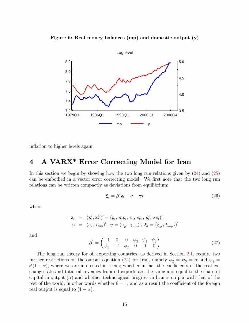
Figure 6: Real money balances (mp) and domestic output (y)

7.2

7.4

7.6

7.8

8.0

8.2

1979Q1 1986Q1 1993Q1 2000Q1 2006Q43.5

4.0

4.5

5.0

Log level

mp y

in�ation to higher levels again.

4 A VARX* Error Correcting Model for Iran

In this section we begin by showing how the two long run relations given by (24) and (25)can be embodied in a vector error correcting model. We �rst note that the two long runrelations can be written compactly as deviations from equilibrium:

�t = �0zt � c� t (26)

where

zt = (x0t;x�0t )0 = (yt, mpt, �t, ept, y�t , xot)

0 ;

c = (cy; cmp)0; = ( y; mp)

0; �t =��yt, �mp;t

�0and

�0=

��1 0 0 2 1 3�1 �1 �2 0 0 0

�(27)

The long run theory for oil exporting countries, as derived in Section 2.1, require twofurther restrictions on the output equation (24) for Iran, namely 2 = 3 = � and 1 =� (1� �), where we are interested in seeing whether in fact the coe¢ cients of the real ex-change rate and total oil revenues from oil exports are the same and equal to the share ofcapital in output (�) and whether technological progress in Iran is on par with that of therest of the world, in other words whether � = 1, and as a result the coe¢ cient of the foreignreal output is equal to (1� �).

15

The VARX*(s; s�) model that embodies �t is constructed from a suitably restricted ver-sion of the VAR in zt. In the present application zt = (x0t;x

�0t )0 is partitioned into the 4� 1

vector of endogenous variables, xt = (yt, mpt, �t, ept) ; and the 2 � 1 vector of the weaklyexogenous variables, x�t = (y

�t , xot)

0. Also as shown in Appendix C, the hypothesis that allthe six variables are I(1) cannot be rejected. Moreover, it is easily established that the twoexogenous variables are not cointegrated. Under these conditions, following Pesaran, Shin,and Smith (2000), the VAR in zt can be decomposed into the conditional model for theendogenous variables:

�xt = ��xzt�1 +s�1Xi=1

i�xt�i +�0�x�t +

s��1Xi=1

�i�x�t�i + a0 + a1t+ �t; (28)

and the marginal model for the exogenous variables:

�x�t =s�1Xi=1

��i�zt�i + b0 + ux�t; (29)

If the model includes an unrestricted linear trend, in general there will be quadratic trendsin the level of the variables when the model contains unit roots. To avoid this, the trendcoe¢ cients are restricted such that a1 = �x�; where � is an 6� 1 vector of free coe¢ cients,see Pesaran, Shin, and Smith (2000) and Section 6.3 in Garratt, Lee, Pesaran, and Shin(2006). The nature of the restrictions on a1 depends on the rank of �x. In the case where�x is full rank, a1 is unrestricted, whilst it is restricted to be equal to 0 when the rank of�x is zero. Under the restricted trend coe¢ cients the conditional model can be written as

�xt = ��x [zt�1 � �(t� 1)] +s�1Xi=1

i�xt�i +�0�x�t +

s��1Xi=1

�i�x�t�i + ~a0 + �t; (30)

where ~a0 = a0 + �x�. We refer to this speci�cation as the vector error correcting modelwith weakly exogenous I(1) variables, or VECX*(s; s�) for short. Note that ~a0 remainsunrestricted since a0 is not restricted. While for consistent and e¢ cient estimation (andinference) we only require the conditional model as speci�ed in (28), for impulse responseanalysis and forecasting we need the full system vector error correction model which alsoincludes the marginal model; as such we need to specify the process driving the weaklyexogenous variables, �x�t .The long run theory imposes a number of restrictions on �x and �. First, for the

conditional model to embody the equilibrium errors de�ned by, (26), we must have �x =�x�

0, which in turn implies that rank(�x) = 2. Furthermore, the restrictions on the trendcoe¢ cients are given by

�x� = �x�0� = :

Since under cointegration �x 6= 0, it then follows that a trend will be absent from the longrun relations if one of the two elements of �0� is equal to zero. These restrictions are knownas co-trending restrictions, meaning that the linear trends in the various variables of thelong run relations gets cancelled out. This hypothesis is important in the analysis of output

16

convergence between domestic and the foreign variables, since without such a co-trendingrestriction the two output series will diverge even if they are shown to be co-integrated.The theory also imposes a number of long run over-identifying restrictions on the elements

of �. The total number of over-identifying restrictions is given by 12�4 = 8, and there are 4structural parameters to be estimated, �; �; �1 and �2. This leaves us with 4 over-identifyingrestrictions to test.

5 Long Run Estimates and Tests

5.1 Order Selection and Deterministic Components

We propose to use the VECX*(s; s�) model de�ned by (30) to test the various long runtheory restrictions set out above. First we need to determine the lag orders s and s� in theVARX*(s; s�) model.4 For this purpose we use the Akaike Information Criterion (AIC) andthe Schwarz Bayesian Criterion (SBC) applied to the underlying unrestricted VARX* model.The results are summarized in Table 1. SBC selects the lag orders s = s� = 1; whilst, as tobe expected, AIC selects a higher order lag for the endogenous variables, namely s = 2 ands� = 1. We follow AIC and base our analysis on the VARX*(2,1), since under-estimatingthe lag orders is generally more serious than overestimating them.

Table 1: Lag order selection criteria

Lag length AIC SBCs = 1 s� = 1 1455.32 1327.48s = 1 s� = 2 1445.35 1277.14s = 2 s� = 1 1459.09 1297.61s = 2 s� = 2 1451.63 1249.78

Notes: AIC refers to the Akaike Information Criterion and SBC refers to the Schwarz Bayesian Criterion.

As to the deterministic variables included in our model we make use of both a constantand a linear trend. As a trend may or may not be found in the long run relations we alsotest for co-trending restrictions given by �0� = 0. We also experimented with including awar and revolution (WR) dummy amongst the determinstics. The WR dummy takes thevalue of 1 between 1979 quarter 1 and 1988 quarter 2 and zeros outside this period, and isintended to capture the joint e¤ects of the 1979 Islamic Revolution and the war with Iraqwhich lasted from September 1980 until August 1988. The WR dummy could also pick upthe e¤ects of economic liberalisation that took place after the ending of the Iran-Iraq war.But as we shall argue in Section 5.2.3 below, once xot, the oil exports variable, is includedin the model the WR dummy ceases to be statistically signi�cant.

4All estimations and test results are obtained using Micro�t 5.0. For further technical details see Pesaranand Pesaran (2009), Section 22.10.

17

5.2 Estimation and Testing of the Long Run Relations

Having established the order of VARX* to be (2,1) we need to determine the number ofcointegrating relations given by r = rank(�x), where �x is de�ned by (30). Cointegrationtests with null hypothesis of no cointegration, one cointegrating relation, and so on are carriedout using Johansen�s maximum eigenvalue and trace statistics as developed in Pesaran, Shin,and Smith (2000) for models with weakly exogenous regressors. The test results are reportedin Table 2. Both the maximal eigenvalue and the trace statistics suggest the presence of twocointegrating relations at the 5 per cent level, which is the same as that suggested by economictheory, thus we set r = 2:

Table 2: Cointegration rank test statistics for the VARX*(2,1) model with en-dogenous variables (y, mp, dp, ep) and the weakly exogenous variables (y*, xo)

H0 H1 Test statistic 95% Critical Values 90% Critical Values(a) Maximal eigenvalue statisticr = 0 r = 1 55.84 41.93 38.29r � 1 r = 2 40.31 33.79 31.23r � 2 r = 3 24.66 26.26 23.93r � 3 r = 4 6.30 17.73 16.08(b) Trace statisticr = 0 r = 1 127.11 90.44 84.24r � 1 r = 2 71.27 60.13 56.47r � 2 r = 3 30.97 36.97 34.02r � 3 r = 4 6.30 17.73 16.08

Notes: The underlying VARX* model is of order (2,1) and contains unrestricted intercept andrestricted trend coe¢ cients. y�t and xot are treated as weakly exogenous, non-cointegrated I(1)variables. The test statistics refer to Johansen�s log-likelihood-based maximum eigenvalue andtrace statistics and are computed using 109 observations from 1979Q4 to 2006Q4.

In order to exactly identify the long run relations, we must impose 4 restrictions, 2restrictions on each of the 2 cointegration relations. The choice of the exactly identifyingrestrictions is econometrically innocuous and is best guided by economic theory. We proceedby taking the �rst cointegrating relation to be the output equation, de�ned by equation (24)and normalised on yt, and the second one the money demand equation, de�ned by (25) andnormalised on mpt = mt�pt. Accordingly, we start with the following two exactly identi�edcointegrating vectors

�0

EX =

��1 0 �13 �14 �15 �16�21 �1 �23 �24 0 �26

�; (31)

where the rows of �0

EX correspond to zt = (yt, mpt, �t, ept, y�t , xot)0. Using this exactly

identi�ed speci�cation we then test the co-trending restrictions, �0� = = ( y; mp)0 = 0.

The log-likelihood ratio (LR) statistic for jointly testing the two co-trending restrictions takesthe value 10.15, and is asymptotically distributed as a chi-squared variate with two degreesof freedom. Therefore, based on the asymptotic distribution the co-trending restrictionsare rejected. But we are working with a relatively large dimensional VARX* model usinga moderate number of time series observations. In such situations it is known that the

18

LR tests could over-reject in small samples (see, for example, Gredenho¤ and Jacobson(2001) as well as Gonzalo (1994), Haug (1996) and Abadir, Hadri, and Tzavalis (1999)).To deal with the small sample problem we computed bootstrapped critical values based on1,000 replications of the LR statistic. Using the observed initial values of each variable, theestimated model, and a set of random innovations, an arti�cial data set is generated foreach of the 1,000 replications under the assumption that the estimated version of the modelis the true data-generating process. For each of the replicated data sets, we �rst estimateour VECX* model subject to the exact identifying restrictions in (31) and then subject tothe two co-trending restrictions. Finally, the empirical distribution of the LR test statisticis derived using the 1,000 replications. Having applied this technique, the bootstrappedcritical value for the joint test of the two co-trending restrictions is 10.20 at the 5 percentlevel, and 15.22 at the 1 percent level, as compared to the LR statistic of 10.15. Hence,based on the bootstrapped critical values the co-trending restrictions cannot be rejected atthe conventional levels of signi�cance, although the outcome of the test at the 5 percent levelis rather marginal and is subject to the random variation of the bootstrapped critical values.We shall, therefore, impose the co-trending restrictions whilst considering the other theoryrestrictions, and return to them to see if they continue to be supported by the data once theother restrictions are imposed.

5.2.1 Testing Long Run Theory Restrictions

We �rst consider the theory restrictions on the output equation whilst maintaining the exactidentifying restrictions on the second long run relation. Initially we impose the restrictionthat the coe¢ cients of ept and xot are the same, namely that in (31) �14 = �16 = �. Weobtain the estimates

1 = 0:6931(0:2183)

; 2 = 3 = � = 0:3140(0:1100)

;

with the LR statistic of 10.52 for testing the three restrictions. The �gures in brackets areasymptotic standard errors. The additional restriction has only marginally increased the LRstatistic and is clearly not rejected. In fact the bootstrapped critical values for the test isnow 11.91 at the 5 percent level and 17.12 at the 1 percent level. The implicit estimate of �given by 0:6931=(1� 0:3140) = 1:01 is very close to unity and the null hypothesis that � = 1cannot be rejected, thus implying that the technological growth in Iran is on par with thato¤ the rest of the world. Under � = 1 we have �15 + �14 = 1, and imposing this additionalrestriction the LR statistic increases only marginally from 10.5181 to 10.5198. However, theestimate of �, representing the share of capital, is relatively low, although not far from whatis being considered in the literature for Iran, for instance see Mojaver (2009) in which heconsiders a range of 0.33 to 0.45 for �. In addition, the coe¢ cient of �t in the long run outputequation is �13 = �14:72 (5:91), which is statistically signi�cant, implying that in�ation hasa negative e¤ect on real output which is not supported by the long run theory. This negativee¤ect suggests ine¢ ciencies in both the institutions and economic policies in Iran and showsthe importance of controlling in�ation for growth promotion in Iran.Consider now the second long run equation. The theory restrictions in terms of the

elements of � in (31) are�24 = 0; and �26 = 0:

19

Imposing these additional restrictions on � yields

� = 1, � = 0:2333(0:0465)

, �13 = � 13:06(4:01)

;

�1 = 0:8277(0:1231)

; �2 = �14:53(6:09)

:

The long run income elasticity of money demand is close to unity and the null hypothesisthat it is equal to 1 cannot be rejected. The e¤ect of in�ation on real money balances is alsonegative and statistically signi�cant. This is in line with our earlier discussion that in�ationin the money demand equation acts as a proxy for the interest rate. In fact it would be aperfect proxy if it can be assumed that the Fisher parity holds in Iran. Imposing �1 = 1 andre-estimating subject to all the seven over-identifying restrictions we obtain

� = 1; � = 0:2647(0:0489)

, �13 = �13:84(4:37)

;

�1 = 1; �2 = �16:37(6:79)

:

The LR statistic for testing all the 7 restrictions jointly is 23.34 which is to be comparedto the bootstrapped critical values of 21.59 and 30.99 at the 5 and 1 percent signi�cancelevels, respectively. Therefore, the restrictions are rejected at 5 percent level, but not atthe 1 percent level. The test outcome is inconclusive and further investigation seems inorder. We considered relaxing some of the restrictions in the real money demand equationand found that the primary source of the rejection of the restrictions is the zero restrictionimposed on the coe¢ cient of the real exchange rate variable. Once this restriction is relaxedthe following estimates are obtained

� = 1; � = 0:2467(0:0600)

, �13 = �12:06(3:36)

;

�1 = 1; �2 = �1:91(2:99)

, �24 = �0:2380(0:0496)

:

There are now six over-identifying restrictions on the long run relations, and the LR statisticfor testing these restrictions is 13.37 as compared to the bootstrapped critical values of 16.29and 19.34 at the 10 and 5 percent signi�cance levels, respectively. Clearly, the restrictionsare not rejected even at the 10 percent signi�cance level. This is reassuring particularlyas far as the long run estimates of the output equation is concerned, since whether �24 isrestricted or not seems to have little e¤ects on the estimates of the output equation, whichis the focus of the present investigation. However, relaxing �24 = 0 does signi�cantly a¤ectthe in�ation elasticity of the money demand which is reduced from �16:37 to �1:91 and isno longer statistically signi�cant.We are presented with a clear choice. Should we maintain the theory restrictions which

are rejected at the 5 percent level, although not at the 1 percent level, or should we opt forthe new speci�cation of the real money demand equation that includes the et � pt variablewhich is di¢ cult to justify in an economically meaningful sense. Given that we are primarilyinterested in the long run e¤ects of oil exports for real output, and the choice of the realmoney demand equation does not seem to play a central role for that issue, in the rest of

20

the paper we shall maintain the theory consistent money demand equation since it is easierto interpret. Also, since the theory restrictions are not rejected at the 1 percent level, ouradherence to a theory consistent real money demand equation is not without some empiricalfoundations.Furthermore, the theory consistent speci�cations are robust to alternative measurements

of foreign output and the exchange rate. For instance, estimating the VECX* model withforeign output computed using �xed weights based on the average of three consecutive years(2001-2003), yield similar outcomes

� = 1; � = 0:2311(0:0432)

, �13 = �17:13(5:08)

;

�1 = 1; �2 = �16:06(6:30)

;

to when we use foreign output based on time-varying weights (y�t ), with the 7 over-identifyingrestriction now not being rejected at the 5 percent signi�cance level.

5.2.2 Free and O¢ cial Exchange Rates

As noted earlier, a similar issue of measurement also arises with respect to the exchangerate. Since the 1979 Revolution the Iranian rial has depreciated signi�cantly against the USdollar under a variety of exchange rate regimes from a �xed rate to multiple rates and backto a uni�ed pegged managed rate. It has depreciated from 70 rials per US dollar in 1979to 9170 rials in 2006, or around 131 fold increase, see Pesaran (1984) and Pesaran (2000).Figure 7 shows (in logs) the free rate (or black market in certain periods), et , and the o¢ cialexchange rate , eOF;t, over the period 1979Q1-2006Q4. The two rates are at par at the startof the Revolution but depart soon thereafter. They are, however, brought in line by twomajor jumps the last of which is associated with the successful uni�cation of the exchangerates during Khatami�s Presidency in 2002.To investigate the robustness of our results to the choice of the exchange rate we employ

a geometrically weighted average of the free and the o¢ cial rates, e!;t = !et + (1� !)eOF;t.The weights ! : (1 � !) are intended to re�ect the proportion of imports by public andprivate agencies that are traded at the two exchange rates, on average. There is little hardevidence on !, although due to the gradual attempts at currency uni�cation, it is reasonableto expect ! to have risen over time. Initially we set ! = 0:75, but smaller values of ! = 0:70and 0:60 resulted in very similar estimates and test outcomes. Using e!;t with ! = 0:75 wecould not reject the 7 over-identifying restrictions even at the 10 percent level, since the LRstatistic is 18.65 as compared to the bootstrapped critical values of 19.10 and 22.67 at the10 and 5 percent signi�cance levels, respectively. For ! = 0:75 we obtained the followingestimates:

� = 1; � = 0:1964(0::0308)

, �13 = �8:97(2:55)

;

�1 = 1; �2 = �16:01(6:84)

;

which yield a smaller capital share of 0.1964 as compared to 0.2647, with the coe¢ cientof in�ation in the output equation still negative and statistically signi�cant. However, the

21

Figure 7: Free and o¢ cial exchange rates

4

6

8

10

1979Q1 1986Q1 1993Q1 2000Q1 2006Q44

6

8

10

Log level

Official Free

in�ation elasticity of money demand, -16.01, is roughly the same as in the case when we usethe �oating exchange rate, et. Given that we do not know what these weights should be, fornow we will proceed by only reporting the results when using the free exchange rate in ourmodel, but we will return to this issue when looking at the short run dynamics.5

5.2.3 Including a War and Revolution Dummy

To see if the model captures the e¤ects of the 1979 Islamic Revolution as well as the war withIraq, which lasted from September 1980 until August 1988 and the economic liberalisationthat followed after the war, we introduce a war and revolution dummy. This dummy takesthe value of unity over the period 1979Q1 to 1988Q2, and zero otherwise. As before boththe maximal eigenvalue and the trace statistics indicate the presence of two cointegratingrelations at the 5 percent level.6 Setting r = 2 and imposing the same over-identifyingrestrictions as in the above Sub-sections, namely:

�0� = = 0;

�14 = �16 = �;

�15 + �14 = 1 =) � = 1;

�21 = 1 =) �1 = 1;

�24 = 0; and �26 = 0;

5We also estimated the VARX* model with e0:75;t and the foreign output variable constructed using �xedweights and obtained very similar estimates. These results are available upon request.

6The inclusion of the dummy variable changes the critical values of the test. The test statistics and theassociated critical values are available on request.

22

and re-estimating subject to the seven over-identifying restrictions we obtain

� = 1; � = 0:2870(0:0647)

, �13 = �20:81(12:57)

;

�1 = 1; �2 = �18:48(14:94)

:

The LR statistic for testing all the 7 restrictions jointly is 24.02 which is to be comparedto the bootstrapped critical values of 22.30 and 29.09 at 5% and 1% signi�cance levels,respectively. Therefore, as before the restrictions are rejected at 5% level, but not at the1% level. The estimates are fairly similar to the case when we do not include the war andrevolution dummy, with the long run negative e¤ects of in�ation on real output still present,although now statistically less signi�cant than previously. Table 3 reports the coe¢ cientof the war and revolution dummy in the error correction equations where we observe thatthe war and revolution dummy is clearly insigni�cant at the 10 percent level in the realexchange rate and the in�ation equations, while it is signi�cant at the 10 percent level forthe real money equation and signi�cant at the 5 percent level in the output equation. Theseestimates suggest only a modest average decline in real output due to revolution and war,once the e¤ects of the declines in real oil exports are taken into account.

Table 3: Reduced-form error correction equations of the VECX*

Equation �yt �mpt ��t �ept

WR Dummy �0:016993�(0:0063355)

�0:0086472��(0:0047351)

0:0045923(0:0039030)

0:0078659(0:026624)

Notes: � denotes signi�cance at the 5 percent level and �� denotes signi�cance at the 10 percent level.

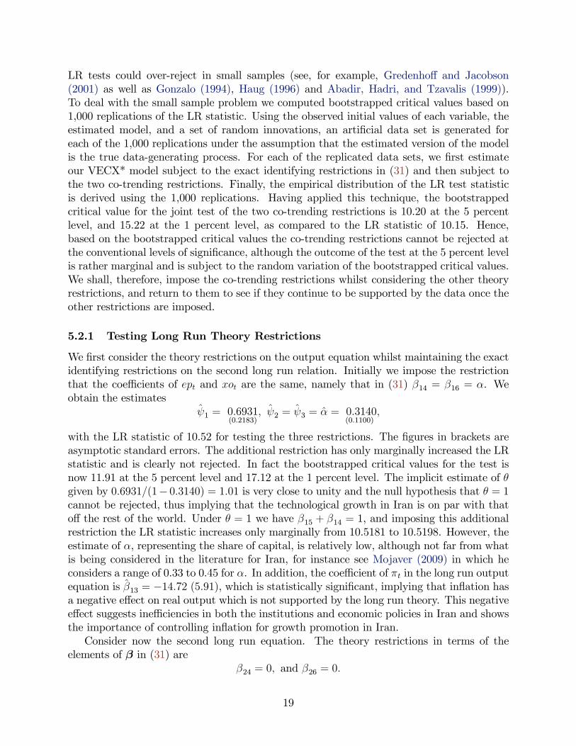
This point is clearly illustrated using Figure 8 which shows the signi�cant drop in oilexports in the aftermath of the revolution, which only begins to recover in a sustainedmanner after the end of the war with Iraq. In e¤ect, the decline in oil exports, partly dueto the economic disruptions, in turn puts further downward pressure on the real economy.Although the price of oil declined slightly and steadily between 1979 and 1986, this was notthe case for Iranian revenues from oil exports which drop signi�cantly after the revolutionand again at the start of the Iran-Iraq war while on the other hand was at a higher levelthan the price of oil after the war. Thus, the negative e¤ects of the war and revolution islargely picked up by the oil export variable, xot.However, if we had followed the literature and instead of total revenue from oil exports,

xot, used the nominal price of oil, pot , in our model, then the war and revolution dummywould have been necessary for modelling the disruptive e¤ects of the revolution and the waron the real economy. In the light of these observations, we will work with the model withthe xot variable included, but without the the war and revolution dummy.

23

Figure 8: Price of oil and revenue from oil exports (xo)

2.0

2.5

3.0

3.5

4.0

4.5

1979Q1 1986Q1 1993Q1 2000Q1 2006Q49.0

10.0

11.0

12.0

13.0

Log level

price of oil xo

5.2.4 Import Weights as Opposed to Trade Weights

We also estimated our model with foreign output computed using import weights, both �xedand time-varying, rather than trade weights. The cointegration rank test statistics for theVARX* (2,1) model with the data vector de�ned by zt =

�yt, mpt, �t, ept, y�t;IM , xot

, where

y�t;IM is real foreign output using time-varying import weights, again suggest the presenceof two long run relations. Imposing the same 7 over-identifying restrictions as before andre-estimating we obtain

� = 1; � = 0:2702(0:0487)

, �13 = �13:79(4:20)

;

�1 = 1; �2 = �16:02(6:47)

:

The LR statistic for testing all the 7 restrictions jointly is now 28.65 which is to be comparedto the bootstrapped critical values of 21.79 and 30.43 at 5% and 1% signi�cance levels,respectively. The results are very similar to the ones reported in the above Sub-sections,and shows that the choice of the weights in the construction of the foreign variable is ofsecond order importance. However, given the important changes that have taken place inthe geographical composition of the Iranian foreign trade since the revolution, graduallyshifting Iran�s trade from the West to the East, in what follows we use the time-varyingtrade weights as in Section 5.2.

6 Short Run Dynamics

The estimated model can also be used to examine the dynamic responses of the Iranianeconomy to various types of shocks, in particular shocks to oil exports and foreign output.

24

Initially, we consider the e¤ects of system wide shocks on the cointegrating relations using thepersistence pro�les, developed by Lee and Pesaran (1993) and Pesaran and Shin (1996). Onimpact the persistence pro�les (PP) are normalized to take the value of unity, but the rate atwhich they tend to zero provide information on the speed with which equilibrium correctiontakes place in response to shocks. The PP could initially over-shoot, thus exceeding unity, butmust eventually tend to zero if the long run relationship under consideration is cointegrating.To investigate the e¤ects of variable speci�c shocks on the Iranian economy we make useof the Generalized Impulse Response Functions (GIRFs), developed in Koop, Pesaran, andPotter (1996) and Pesaran and Shin (1998). Unlike the orthogonalized impulse responsespopularized in macroeconomics by Sims (1980), the GIRFs are invariant to the ordering ofthe variables in the VARX* model.

6.1 Persistence Pro�les

Figure 9 depicts of the e¤ect of a system-wide shock to the cointegrating relations with 95percent bootstrapped con�dence bounds. The speed of convergence to equilibrium for thetwo cointegrating relations are quite fast as compared, for example, with the UK (Garratt,Lee, Pesaran, and Shin (2006)) and Switzerland (Assenmacher-Wesche and Pesaran (2008)).The half life of the shock is less than one quarter and the life of the shock is generally lessthan eight quarters. Thus the e¤ect of shocks tend to disappear rather quickly. This could bedue to lack of access to capital markets and an absence of a developed domestic capital andmoney markets, which allows little possibility for shock absorptions. The recently createdOil Stabilization Fund could, in principle, if used appropriately act as a shock absorber whichmight lead to a more sluggish response of the economy to shocks.

6.2 Generalized Impulse Responses

Generalized Impulse Response Functions (GIRFs) can be computed for shocks to any of thevariables in the model, but they are more straightforward to interpret in the case of shocksto the exogenous variables, namely oil exports and foreign output. Consider �rst the GIRFsof a unit shock (equal to one standard error) to oil exports given in Figure 10. These �guresclearly show that a positive shock to oil exports signi�cantly increases in�ation, strengthensthe real exchange rate (et � pt), increases real output, but its e¤ect on real money balanceswhilst positive it is not statistically signi�cant. These results are as to be expected, butalso show that the e¤ects of the shock work themselves through the economy rather rapidly.Note also that these e¤ects tend to be permanent, due to the presence of unit roots in theunderlying variables. Quantitatively, the positive oil export shock increases in�ation by 0.8percent per annum, real output by 3.2 percent and results in a real exchange rate appreciationof around 7.6 percent. The rise in the real exchange rate in the aftermath of the positiveshock to oil exports can also be viewed as supporting the Dutch disease, although here therise in the real exchange rate is in fact accompanied with a rise in real output which doesnot sit comfortably with those that view the Dutch disease as a resource curse.7

7For a short run macroeconomic analysis where a rise in oil exports induces a rise in real output seePesaran (1984).

25

Figure 9: The persistence pro�les of the e¤ect of a system-wide shock to thecointegrating relations with 95 percent bootstrapped con�dence bounds

0.0

0.2

0.4

0.6

0.8

1.0

1.2

0 6 12 18 24

 Output equation

0.0

0.2

0.4

0.6

0.8

1.0

1.2

0 6 12 18 24

Money demand equation

26

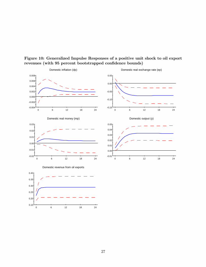
Figure 10: Generalized Impulse Responses of a positive unit shock to oil exportrevenues (with 95 percent bootstrapped con�dence bounds)

­0.004

­0.002

0.000

0.002

0.004

0.006

0.008

0 6 12 18 24

Domestic inflation (dp)

­0.15

­0.10

­0.05

0.00

0.05

0 6 12 18 24

Domestic real exchange rate (ep)

­0.02

­0.01

0.00

0.01

0.02

0.03

0 6 12 18 24

Domestic real money (mp)

­0.01

0.00

0.01

0.02

0.03

0.04

0.05

0 6 12 18 24

Domestic output (y)

0.15

0.20

0.25

0.30

0.35

0.40

0 6 12 18 24

Domestic revenue from oil exports

27

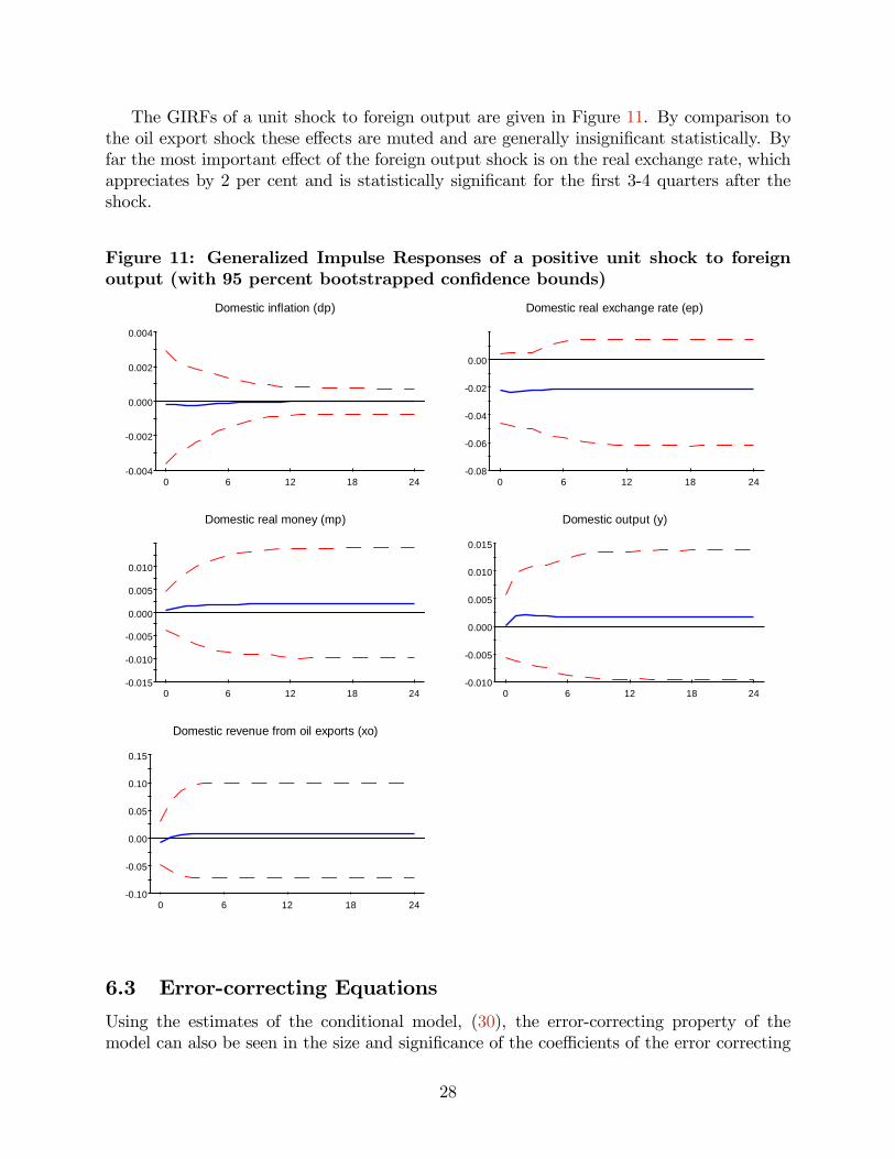
The GIRFs of a unit shock to foreign output are given in Figure 11. By comparison tothe oil export shock these e¤ects are muted and are generally insigni�cant statistically. Byfar the most important e¤ect of the foreign output shock is on the real exchange rate, whichappreciates by 2 per cent and is statistically signi�cant for the �rst 3-4 quarters after theshock.

Figure 11: Generalized Impulse Responses of a positive unit shock to foreignoutput (with 95 percent bootstrapped con�dence bounds)

­0.004

­0.002

0.000

0.002

0.004

0 6 12 18 24

Domestic inflation (dp)

­0.08

­0.06

­0.04

­0.02

0.00

0 6 12 18 24

Domestic real exchange rate (ep)

­0.015

­0.010

­0.005

0.000

0.005

0.010

0 6 12 18 24

Domestic real money (mp)

­0.010

­0.005

0.000

0.005

0.010

0.015

0 6 12 18 24

Domestic output (y)

­0.10

­0.05

0.00

0.05

0.10

0.15

0 6 12 18 24

Domestic revenue from oil exports (xo)

6.3 Error-correcting Equations

Using the estimates of the conditional model, (30), the error-correcting property of themodel can also be seen in the size and signi�cance of the coe¢ cients of the error correcting

28

terms, �t = (�t;y; �t;mp)0, de�ned by (26). The estimates of the reduced form error correction

equations are given in Table 4, from which we can see that �t�1;y and �t�1;mp are bothstatistically signi�cant in the output and real exchange rate equations but not in the realmoney and in�ation equations. There seems to be a dichotomy between the real and the�nancial sides of the economy as far as their responses to disequilibria are concerned withthe real output and real exchange rate adjusting most to shocks.

Table 4: Reduced-form error correction equations of the VECX*

Equation �yt �mpt ��t �ept�y;t�1

0:089�

(0:029)0:026(0:021)

0:028(0:018)

�0:401�(0:118)

�mp;t�1�0:047�(0:023)

0:011(0:017)

�0:008(0:014)

0:332�

(0:093)

�yt�10:325�

(0:094)0:086(0:069)

�0:038(0:058)

�0:184(0:386)

�mpt�1�0:515�(0:174)

0:052(0:128)

0:061(0:106)

0:542(0:711)

��t�1�0:021(0:167)

0:232��

(0:123)�0:143(0:102)

0:335(0:681)

�ept�1�0:082�(0:023)

�0:016(0:017)

�0:001(0:014)

�0:042(0:094)

�y�t0:073(0:547)

0:111(0:402)

�0:036(0:334)

�4:162��(2:235)

�xot0:023��

(0:014)0:009(0:010)

0:004(0:008)

0:027(0:056)

intercept �0:363�(0:144)

�0:005(0:106)

�0:089(0:088)

2:157�

(0:591)

�R2 0:189 0:226 0:138 0:085�R2-AR(p) 0:054

(p=1)0:158(p=2)

0:141(p=2)

0:00(p=1)

SC: �2(4) 0:71 7:95 11:74 8:17FF : �2(1) 3:49 0:57 2:18 11:27N : �2(2) 1:97 2:96 9:56 3354:6HS : �2(1) 0:22 3:45 9:55 19:91

Notes: The two error correction terms are given by:

�y;t = yt + 13:84(4:37)

�t � 0:2647(0:0489)

ept � 0:7353(0:0489)

y�t � 0:2647(0:0489)

xot

�mp;t = mpt � yt + 16:37(6:79)

dpt

�denotes signi�cance at the 5 percent level and �� denotes signi�cance at the 10 percent level. SC is atest for serial correlation, FF a test for functional form, N a test for normality of the errors and HS atest for heteroscedasticity. Critical values are 3.84 for �2(1), 5.99 for �2(2) and 9.49 for �2(4). �R2 is theadjusted squared multiple correlation coe¢ cient, and �R2-AR(p) refers to the �R2 of a univariate autoregressiveequation. The sample period is 1979Q1 to 2006Q4.

Turning to the �t of the error-correcting equations, the in�ation and the real moneybalances equations seem to be the least satisfactory. In the case of the in�ation equationsnone of the regression coe¢ cients are statistically signi�cant and it su¤ers from residual

29

serial correlation.8 In the case of the real money balances the only signi�cant coe¢ cient isthat of the lagged in�ation which is signi�cant at the 10 percent level. The �t of the realexchange rate equation seems reasonable, considering the general unpredictably of exchangerates documented in the literature. By contrast the output equation provides a reasonableexplanation, particularly considering the signi�cant disruptions experienced by the Iranianeconomy over the period under study and the fact that no dummy variables are included inthe regressions.To evaluate the importance of the error correction terms we also estimated univariate au-

toregressive moving average (ARMA) time series equations for the four endogenous variablesin the VARX* model and concluded that an AR(1) speci�cation �ts best for the real outputgrowth (�yt), and the real exchange rate changes (�ept), and an AR(2) speci�cation forchanges in in�ation (��t) and real money balances ( �mpt): The adjusted squared multiplecorrelation coe¢ cient of these univariate equations are denoted by �R2-AR(p), which needsto be compared to the �R2 of the error correction equations also presented in Table 4. Itis clear that the �t of the ECM equation for output at 19 percent is substantially betterthan the �t of the associated univariate AR(1) equation of only 5.4 percent. The ECM ofthe real exchange rate (at 8.5 percent) also �ts much better than the univariate equation(at 0 percent). By contrast the ECM equations for in�ation and the real money balancesare either worse or not that much better than the univariate alternatives. This seems to belargely due to the fact that the univariate speci�cations point to a higher order dynamicsfor these variables. Unfortunately the available data does not allow us to experiment witha VARX*(3,1) or VARX*(3,2) speci�cations that might be needed to accommodate suchhigher order dynamics.The actual and �tted values for each of the four equations together with the associated

residuals are displayed in Figures 12 . We observe that while there are some large outliers,especially for the exchange rate equation in the mid 1980�s and the beginning of the 1990�sand for output and real money in the early 1990�s, the �tted values seem to track the mainmovements of the dependent variables reasonably well. The presence of large outliers arere�ected in the massive rejection of the normality of the errors in the case of the real exchangerate equation.

8The in�ation equation also seems to su¤er from multicollinearity since despite the fact that none of itscoe¢ cients are statistically signi�cant the overall �t of the equation is highly signi�cant.

30

Figure 12: Actual, �tted, and residuals for the core equations

(a) Output equation

­0.10

­0.05

0.00

0.05

0.10

1979Q4 1986Q3 1993Q2 2000Q1 2006Q4

Actual and fitted

dy fitted­0.10

­0.05

0.00

0.05

0.10

1979Q4 1986Q3 1993Q2 2000Q1 2006Q4

Residuals

(b) Real money demand equation

­0.10

­0.05

0.00

0.05

0.10

1979Q4 1986Q3 1993Q2 2000Q1 2006Q4

Actual and fitted

dmp fitted­0.10

­0.05

0.00

0.05

0.10

1979Q4 1986Q3 1993Q2 2000Q1 2006Q4

Residuals

(c) In�ation equation

­0.10

­0.05

0.00

0.05

0.10

1979Q4 1986Q3 1993Q2 2000Q1 2006Q4

Actual and fitted

ddp fitted­0.06

­0.04

­0.02

0.00

0.02

0.04

1979Q4 1986Q3 1993Q2 2000Q1 2006Q4

Residuals

(d) Real exchange rate equation

­0.5

0.0

0.5

1.0

1979Q4 1986Q3 1993Q2 2000Q1 2006Q4

Actual and fitted

dep fitted­0.5

0.0

0.5

1.0

1979Q4 1986Q3 1993Q2 2000Q1 2006Q4

Residuals

31

7 Concluding Remarks

This paper makes a theoretical contribution by showing the conditions under which incomefrom a resource can have a lasting impact on growth and per capita income. Using thistheoretical insight, it provides a small quarterly model of the Iranian economy, as an exampleof a major oil exporting economy, where the long run implications of oil exports for realoutput, in�ation, real money balances, and the real exchange rate are tested. The resultsare generally supportive of the long run theory, although they point to certain ine¢ ciencies inthe demand management of the economy that manifest themselves as a signi�cantly negativee¤ect of in�ation on real output, even in the long run. The estimates also suggest a ratherrapid response of the economy to shocks, which could be due to the relatively underdevelopednature of the money and capital markets in Iran. Such markets tend to act as shock absorbersin developed economies during normal conditions, although as we have seen recently, theycan also act as shock magni�ers during crisis periods.The research in this paper can be extended in a number of directions. The current

VARX* model is connected to the rest of the world through oil exports and foreign realoutput. Although these are clearly the most important channels of the transmission ofshocks to the Iranian economy, there could be others. It would be interesting to see if themodel can be linked to the global model recently developed in Dees, di Mauro, Pesaran,and Smith (2007), where the di¤erential e¤ects of supply and demand shocks and di¤erentregional shocks on the Iranian economy could be investigated.It would also be of interest to investigate the extent to which the long run e¤ects of oil

exports on real output documented in this paper can be found in the case of other major oilexporters. However, to obtain a su¢ ciently long quarterly series, and to take into accountthe particular institutional features of these economies, will present some challenges. Thetheoretical results of the paper can also be extended to allow for interactions between the oiland non-oil sectors and the short term e¤ects of oil price volatility. Such an extension could,for example, help shed light on the importance of the recently established Oil StabilizationFund in Iran or the sovereign wealth funds formed in other oil exporting countries as shockabsorbers.

32

Appendix A: Macroeconometric Models of the IranianEconomy - A Survey of the Literature

The origins of macro-econometric modeling in Iran date back to the early 1970�s, whenHabib-Agahi (1971)9 pioneered the practice at the Iranian Plan and Budget Organization(PBO). Habib-Agahi�s model contained 8 linear behavioral relations and 7 accounting iden-tities, linking 3 categories of imports, aggregate output, real disposable income, private andgovernment consumption and investment expenditures to the size of the development bud-get, oil and non-oil exports, and foreign loans for development. The model was estimatedusing annual time series data over the 1959-1970 period, and formed the basis of the �rst"o¢ cial" macro-econometric model to be developed by the PBO. This was a modest exercisein macro-econometric modeling, largely re�ecting the data and computational limitationsprevailing in Iran at the time.Looking to other models subsequently developed at the PBO, a distinction needs to

be made between the models that were constructed before the 1979 revolution and thoseconstructed afterwards. The �rst model developed at the PBO before the revolution wasa modi�cation of Habib-Agahi�s model and related non-oil exports to the value added inagriculture instead of treating it as exogenous. However, the value added in agriculture wasnow assumed to be exogenous. The second major macro-econometric model constructed atthe PBO before the revolution was much more detailed, and represented important advancesover the earlier one. It allowed for the e¤ect of relative prices on imports and non-oil exportsdemands, contained equations for the determination of a number of key monetary aggregatesand tax revenues, and used a Phillips type wage equation to close the model. The model wasestimated over the period 1961-1975 and was the �rst serious empirical attempt at modelingthe interactions of the monetary and real variables in the Iranian economy. However, as withthe other models developed for the Iranian economy there is no systematic documentationof the model�s short run predictive performance or its long run properties.Perhaps not surprisingly, revolution and the subsequent eight-year war with Iraq halted

any serious development of macro-econometric models both inside and outside of the PBO.But with the ending of the Iran-Iraq war in 1988, and the government�s attempt at regener-ation and reconstruction of the economy, once again the problem of economic planning andthe development of appropriate macro-econometric models gained priority. But althoughthe importance of macro-econometric models was recognized in the formulation of the FirstFive-Year Development Plan (1990-94), given the urgency surrounding the formulation ofthe First Plan and the limited time available to accomplish the task, serious attempts atmacro-econometric modeling had to wait until after its approval and implementation.According to o¢ cial accounts, two di¤erent macro-econometric models were utilized in

the formulation of the Second Five-Year Development Plan.10 The �rst model, PBO1, con-tains 25 econometrically estimated behavioral, technical, and institutional relations and a

9The dates in the 1300s are based on the Iranian calendar. The corresponding Gregorian dates are roughlyequal to the Iranian date plus 621. Publications in Persian are cited with the Gregorian dates in the textbut with both the Iranian and the Georgian calendar dates in the references.10See PBO (1993). Initially the implementation of the Second Five Year Development Plan was intended

to commence in March 1994, but due to delay in its approval by the Iranian Parliament was postponed byone year.

33

number of accounting identities. With a few exceptions these relations are estimated bythe least squares methods over the period 1974-1993, and are documented in PBO (1993).11

This model is composed of a production and factor demand module, a Keynesian income-expenditure �ow module, with investment expenditures disaggregated by 10 major produc-tion sectors, and an aggregate price equation. The second model developed seems to representan extension of the �rst.In addition to these models used for Iran�s development plans, a number of other macro-

econometric models have been developed for Iran since the contribution of Habib-Agahi inthe beginning of the 1970�s, both at the PBO and by other researchers around the world.Prominent examples of the latter category are the models developed by Baharie (1973), Vakil(1973), Shahshahani-Madani (1978), Heiat (1986) and Safai (1986). These models di¤er inthe extent of detail and the level of disaggregation, but are very similar in their underlyingstructures. They are largely demand-determined Keynesian models, and with a few minorexceptions neglect the e¤ect of relative prices and stock-�ow relations on the economy�sevolution. Also, very little is known about their short run forecasting performance, or theirlong-term properties. In contrast to these papers, Noferesti and Arabmazar (1993) developa model in which aggregate supply is not assumed to be perfectly elastic, while Valadkhani(1997), building on the work of the above-mentioned papers, develops a more comprehensivemacroeconometric model for Iran.There are also a number of simple planning/optimal control models developed notably

by Motaman (1979), Razavi (1982), and Razavi (1983) for the analysis of the optimal rate ofoil production in oil-based economies. These models are primarily concerned with the inter-temporal optimization problem involved in oil production decisions (namely, whether toproduce now or later), and are typically very simple as far as their main structural relationsare concerned. They are not intended as forecasting or budgetary tools and, in view ofthe current constraints on Iran�s capacity to produce oil, have limited relevance to Iran�seconomic policy problems.An alternative strategy to the models developed in the above mentioned papers would be

to estimate vector autoregressive (VAR) models in some of the main macroeconomic vari-ables, such as output, price level, money supply, oil exports, consumption, and investment,along the lines originally developed by Sims (1980). In more recent papers, Mehrara andOskoui (2007) make use of a structural VAR to determine whether oil price shocks are themain source of output �uctuation for Iran, while Elyasiani and Zhao (2008) make use ofvector autoregression, generalized impulse response function and generalized variance de-composition techniques to determine the interdependencies of Iran with its major tradingpartners and the US. But the use of VAR models, without imposition of structural relationson their long run solutions, will be limited to short-term forecasting and are unlikely to berelevant for medium term policy analysis. Thus, a long run structural approach to VARmodeling and its application to the Iranian economy, which we take up in this paper, areworth pursuing.Other papers of interest dealing with economic growth in Iran are those of Valadkhani

(2006), which looks at the determinants of the growing unemployment rate in Iran, Pahla-vani, Wilson, and Worthington (2005), which tries to identify the short and long run deter-

11The relations in the published version of model PBO1 were mainly estimated over the period 1974-1992.

34

minants of growth, taking into account the endogenously identi�ed structural breaks in Iran,and Becker (1999), which looks at the development of several variables from pre- to post-revolution and the e¤ect of monetary shocks on these variables. Bahmani-Oskooee (1995)and Kia (2006) explore the determinants of in�ation in Iran, taking into account the roleexternal factors.While all the papers discussed so far have made use of annual data, there are a few

IMF working papers on Iran using quarterly data. In particular, Bonato (2008) looks atthe determinants of in�ation in Iran, Celasun and Goswami (2002) develop an econometricmodel of short run in�ation and long run money demand dynamics in Iran, and Liu andAdedeji (2000) construct a model to develop the determinants of in�ation in Iran. However,all of the papers using quarterly data focus on a certain aspect of the Iranian economy, forinstance the money demand relation or the determination of in�ation, and as such do notconsider the interconnection of the domestic variables with that of foreign variables. Neitherdo they explore the short run and the long run channels of growth. Part of our contributionhas then been to make use of quarterly data, while exploring the interconnection betweenthe Iranian economy and the rest of the world and paying attention to both the short andlong run channels through which oil export revenues e¤ect growth.

Appendix B: Sources and Construction of the Data

Domestic and Foreign Data Series

Our data set contains quarterly observations on Iran and another 33 countries, from the�rst quarter of 1979 to the fourth quarter of 2006. The domestic variables included are(log) real output, yt, (log) real money supply, mpt, (log) price level, pt, the rate of in�ation,�t = pt � pt�1, and (log) nominal exchange rate, et. Speci�cally

yt = ln(GDPt=CPIt), mpt = log(Mt=CPIt),

et = ln(Et), pt = ln(CPIt), (32)

where GDPt is the nominal Gross Domestic Product, Mt is a broad liquidity measure thatincludes M1 and Quasi Money, CPIt is the consumer price index, and Et is the number ofrials per one US dollar exchanged on �free�markets.The two exogenous variables in the model are foreign output, y�t , and oil income in US

dollars de�ned as xot = ln(P ot Xot ), where P

ot is the nominal price of oil per barrel in US

dollars, and Xot is the domestic oil export in thousands of barrels per day. Foreign output

was computed as the trade weighted average of log real output indices (yjt) of Iran�s tradingpartners:

y�t =33Xj=1

�!j;t�1yjt; time varying weights,

y�t;FW =33Xj=1

!j;2001�03yjt; �xed weights,

35

where !j;2001�03 and �!j;t�1 are de�ned below by (33) and (34). The countries includedin these weighted averages are: Argentina, Australia, Austria, Belgium, Brazil, Canada,China, Chile, Finland, France, Germany, India, Indonesia, Italy, Japan, Korea, Malaysia,Mexico, Netherlands, Norway, New Zealand, Peru, Philippines, South Africa, Saudi Arabia,Singapore, Spain, Sweden, Switzerland, Thailand, Turkey, United Kingdom, and UnitedStates.The trade weights are computed based on the IMF Direction of Trade Statistics between

1980 and 2006. The bilateral trade of Iran with country j during a given year t, denotedby Tjt, is calculated as the average of exports and imports of Iran with that country. Tradedata for Belgium is only available from 1997, and so the trade shares for Belgium between1980 and 1996 was calculated by using the data on Belgium-Luxembourg and multiplyingit by 0.93 (this procedure was also adopted in Dees, di Mauro, Pesaran, and Smith (2007)).In addition, trade data between South Africa and partner countries are only available from1998, and so the data of all trading partners with South Africa was used to construct theSouth African trade shares with partners between 1980 and 1997.The �xed trade weights were computed over the period 2001-2003 and are given by

!j;2001�03 =Tj;2001 + Tj;2002 + Tj;2003T2001 + T2002 + T2003

; (33)

where Tt =PN

j=1 Tjt, for t = 2001; 2002; 2003: The time varying trade weights are computedas

�!jt =Tj;t + Tj;t�1 + Tj;t�2Tt + Tt�1 + Tt�2

(34)

We also considered three year moving averages of the the annual trade shares, !jt = Tjt=Ttand obtained very similar results.The most important trading partner for Iran is Japan, which accounts for between 15 and

20 percent of the total Iranian trade. More than 40 percent of the Iranian trade originatesin or is destined for the euro area economies with Germany, Italy and France being Iran�smost important trading partners in Europe.12 Trade with China has increased signi�cantlyover the past two decades, emphasising the shift in the Iranian trade from the west to theeast. Other countries in our data set with whom Iran�s total trade is more than �ve percentare UK, Korea, and Turkey.

Data Sources: Domestic Variables

Real Output

The main source of data on Iran�s real output is the Central Bank of the Islamic Republicof Iran (CBI) online database: Economic Time Series Database (http://tsd.cbi.ir/). Quar-terly observations are available from 1988Q2 while annual data is available from 1959. Weseasonally adjust the quarterly data using the U.S. Census Bureau�s X-12 ARIMA seasonal

12When computing the trade weights and thus the foreign variables we aggregate Austria, Belgium, Fin-land, France, Germany, Italy, Netherlands, and Spain as the euro countries and so use their combined tradeweight and output.

36

adjustment program.13 Quarterly series were interpolated (backwards) linearly from the an-nual series using the same method as that applied by Dees, di Mauro, Pesaran, and Smith(2007) to data for a number of the 33 countries in their data set. This data source is alsoupdated to end of 2006 and used for the computation of the foreign output variable describedabove. For a description of the interpolation procedure see Dees, di Mauro, Pesaran, andSmith (2007) Section 1.1 of Supplement A.

Consumer Price Indices

The CBI online database contains annual CPI data from 1959Q2 and quarterly data from1990Q2. To complete the quarterly data series we make use of several volumes of the CBI�sEconomic Report and Balance Sheets. We �rst use the 1981, 1987, and the 1989 EconomicReport and Balance Sheets to compute quarterly data between 1976 and 1989 from themonthly data available in these reports. We then obtain quarterly CPI series by splicingthe three series of CPI such that our quarterly CPI data stretches from 1976Q2 to 2007Q1,setting the average value of the index for 2000 equal to 100. Finally, we seasonally adjust thequarterly data using the U.S. Census Bureau�s X-12 ARIMA seasonal adjustment program.

Exchange Rates

We obtain the o¢ cial exchange rate series from the CBI online database. This data isavailable from 1959Q2. The nominal �market�or �free�exchange rate series used is from theIMF INS database and is available from 1979Q1.

Money and Quasi Money

The data on money and quasi money supply are from the IMF IFS series 34 and 35 and areavailable from 1957Q1. As money supply data between 1984Q2 and 1986Q2 is missing inthe IFS series, we obtained the complete series by splicing the IFS and CBI data on moneysupply. Quasi money data was missing for 1960Q4, 1978Q4, and between 1985Q2 to 1986Q2.Again we �lled in for the missing data by splicing the IFS and the CBI data, but as CBIdata was only available from 1974Q1, the complete series for quasi money is available onlyfrom 1961Q1.We seasonally adjust the quarterly data on money and quasi money supply using the

U.S. Census Bureau�s X-12 ARIMA seasonal adjustment program.

Oil Exports and Prices

Annual and quarterly oil export (thousand barrels per day) are available, from 1973 and1978Q2 respectively, from the CBI online database. Quarterly crude oil production is alsoavailable from the CBI online database.Value added of oil group, Gross Domestic Product at Basic Prices, and Non-Oil Gross Do-

mestic Product at Basic Prices are available annually from 1959 and quarterly from 1988Q2.

13For further information see U.S. Census Bureau (2007): X-12-ARIMA Reference Manual athttp://www.census.gov/srd/www/x12a/

37

We �rst seasonally adjust the quarterly data and then obtain quarterly series from 1959Q2by linearly interpolating (backwards) the �missing�quarterly series from the annual series

Population

The annual data on population was obtained from the IMF IFS series 99. This data wasavailable from 1948. As quarterly data on population were not available, quarterly serieswere interpolated linearly from the annual series using the same method used to generatequarterly output series described above.

Conversion from Iranian to Gregorian Years

The Iranian year generally starts on the 21st of March, as such the Iranian quarter 1 contains10 days of the Gregorian quarter 1 and 80 days of Gregorian quarter 2. To convert the datafrom Iranian to Gregorian calendar we simply adopt the following rule: G(Q) = 8

9Iran(Q�

1) + 19Iran(Q), where G(Q) is the Gregorian quarter Q and Iran(Q) is the Iranian quarter

Q. More complex ways of calculating, such as taking into account exact number of days inthe Iranian Quarter and converting the data was also investigated, but there were essentiallyno di¤erences in the series.

Appendix C: Unit Root Test Results

To make sure that we make sensible interpretation of the long run relations and also to ensurethat we do not work with a mixture of I(1) and I(2) variables we need to consider the unitroot properties of the core variables in our model (yt;mpt; �t; ept; y�t ; xot). Table 5 reports thestandard Augmented Dickey-Fuller (ADF) test. But as the power of unit root tests are oftenlow we also report the generalized least squares version of the Dickey-Fuller test (ADF-GLS)proposed by Elliott, Rothenberg, and Stock (1996) and the weighted symmetric ADF test(ADF-WS) of Park and Fuller (1995), as they both have been shown to have better powerproperties than the ADF test.It is clear from Figures 2 to 6 that most of the core variables are trended and so we will

include a trend and an intercept in the ADF regression for all the variables but ept and xot,while we will only include an intercept in the ADF regressions applied to their di¤erencesand second di¤erences. As can be seen from Table 5 both ADF and ADF-WS providesstrong support that yt, mpt, �t, ept, y�t , xot are all I(1), as the unit root hypothesis is clearlyrejected when applied to the �rst di¤erences of these variables while this is not the case forthe unit root test applied to the levels. The ADF-GLS on the other hand gives less clear cutresults but generally supports the rejection of unit roots in the �rst di¤erence of the corevariables. Thus we can safely regard all the core variables as being I(1) and not worry aboutdealing with a mixture of I(1) and I(2) variables in our model.

38

Table 5: Unit root test statistics (based on AIC order selection)

Unit root test statistics for the levelsyt pt et ept mpt y�t xot CV CV T

ADF -2.67 -2.01 -0.79 -1.43 -0.19 -1.80 -2.50 -2.89 -3.45ADF-GLS -1.29 -2.01 -1.08 -1.37 -0.68 -2.02 -1.10 -2.14 -3.03ADF-WS -1.48 -2.06 -1.02 -1.72 -0.59 -2.12 -3.09 -2.55 -3.24Unit root test statistics for the �rst di¤erences

�yt �pt �et �ept �mpt �y�t �xot CV CV TADF -8.42 -3.82 -10.35 -10.45 -4.31 -3.37 -8.36 -2.89 -3.45ADF-GLS -7.66 -2.96 -9.79 -10.29 -2.94 -1.94 -1.09 -2.14 -3.03ADF-WS -8.16 -4.04 -10.63 -10.73 -4.29 -3.64 -6.08 -2.55 -3.24Unit root test statistics for the second di¤erences

�2yt �2pt �2et �2ept �2mpt �2y�t �2xot CV CV TADF -9.07 -5.95 -7.78 -7.55 -6.90 -8.79 -10.12 -2.89 -3.45ADF-GLS -3.72 -5.43 -7.82 -7.55 -2.10 -1.50 -0.28 -2.14 -3.03ADF-WS -9.38 -5.84 -8.08 -7.82 -6.77 -8.69 -6.33 -2.55 -3.24

Notes: ADF denotes the Augmented Dickey-Fuller Test, ADF-GLS the generalized least squaresversion of the ADF test, and ADF-WS the weighted least squares ADF test. The sample periodruns from 1979Q1 to 2006Q4. CV T gives the 95 percent simulated critical values for the test withintercept and trend, while C is the 95 percent simulated critical values for the test including anintercept only.

References

Abadir, K., K. Hadri, and E. Tzavalis (1999). The In�uence of VAR Dimensions on Esti-mator Biases. Econometrica 67, 163�181.

Amuzegar, J. (1997). Iran�s Economy under the Islamic Republic. I.B. Tauris.

Amuzegar, J. (2008). Iran�s Oil as a Blessing and a Curse. The Brown Journal of WorldA¤airs 15, 46�61.

Assenmacher-Wesche, K. and M. H. Pesaran (2008). A VECX* Model of the Swiss Econ-omy. Cambridge Working Papers in Economics 0809 .

Baharie, N. (1973). Economic Policy and Development Strategy in Iran: A Macro-Simulation Approach. Ph. D. thesis, University of Illinois, Illinois.

Bahmani-Oskooee, M. (1995). Source of In�ation in Post-Revolutionary Iran. InternationalEconomic Journal 9.2, 61�72.

Becker, T. (1999). Common Trends and Structural Change: A Dynamic Macro Model forthe Pre- and Postrevolution Islamic Republic of Iran. IMF Working Paper WP/99/82.

Binder, M. and M. Pesaran (1999). Stochastic Growth Models and Their EconometricImplications. Journal of Economic Growth 4, 139�183.

39

Bonato, L. (2008). Money and In�ation in the Islamic Republic of Iran. Review of MiddleEast Economics and Finance 4 (1), Article 3.

BP (2009). BP Statistical Review of World Energy: June 2009. Beacon Press.

Brunnschweiler, C. N. and E. H. Bulte (2008). The resource curse revisited and revised:A tale of paradoxes and red herrings. Journal of Environmental Economics and Manage-ment 55 (3), 248 �264.

Caselli, F. and T. Cunningham (2009). Leader behaviour and the natural resource curse.Oxford Economic Papers Forthcoming.

Celasun, O. and M. Goswami (2002). An Analysis of Money Demand and In�ation in theIslamic Republic of Iran. IMF Working Paper WP/02/205.

Collier, P. and A. Hoe­ er (2004). Greed and grievance in civil war. Oxford EconomicPapers 56, 563�595.

Corden, W. M. and J. P. Neary (1982). Booming Sector and De-Industrialisation in a SmallOpen Economy. The Economic Journal 92 (368), 825�848.

Dees, S., F. di Mauro, M. H. Pesaran, and L. V. Smith (2007). Exploring The InternationalLinkages Of The Euro Area: A Global Var Analysis. Journal of Applied Econometrics 22,1�38.

Elliott, G., T. J. Rothenberg, and J. H. Stock (1996). E¢ cient Tests for an AutoregressiveUnit Root. Econometrica 64, 813�836.

Elyasiani, E. and W. Zhao (2008). International interdependence of an emerging market:the case of Iran. Applied Economics 40, 395 �412.

Esfahani, H. S. and M. H. Pesaran (2009). The Iranian Economy in the Twentieth Century:A Global Perspective. Iranian Studies 42, 177 �211.

Garratt, A., K. Lee, M. H. Pesaran, and Y. Shin (2003). A Long Run Structural Macro-econometric Model of the UK. Economic Journal 113, 412�455.

Garratt, T., K. Lee, M. H. Pesaran, and Y. Shin (2006). Global and National Macroecono-metric Modelling: A Long Run Structural Approach. Oxford: Oxford University Press.

Gonzalo, J. (1994). Five alternative methods of estimating long-run equilibrium relation-ships. Journal of Econometrics 60 (1-2), 203 �233.

Gredenho¤, M. and T. Jacobson (2001). Bootstrap Testing Linear Restrictions on Cointe-grating Vectors. Journal of Business and Economic Statistics 19, 63�72.

Habib-Agahi, H. (1971). A Macro Model for Iranian Economy: 1338-1349. Plan and BudgetOrganization, Tehran, Iran.

40

Haug, A. (1996). Tests for cointegration A Monte Carlo comparison. Journal of Economet-rics 71, 89�115.

Heiat, A. (1986). An Econometric Study of an Oil-Exporting Country: The Case of Iran.Ph. D. thesis, Portland State University, Portland, Oregon.

Kia, A. (2006). De�cits, debt �nancing, monetary policy and in�ation in developing coun-tries: Internal or external factors?: Evidence from Iran. Journal of Asian Economics 17 (5),879 �903.

Koop, G., M. H. Pesaran, and S. M. Potter (1996). Impulse Response Analysis in NonlinearMultivariate Models. Journal of Econometrics 74, 119�147.

Krugman, P. (1987). The narrow moving band, the Dutch disease, and the competitiveconsequences of Mrs. Thatcher : Notes on trade in the presence of dynamic scale economies.Journal of Development Economics 27 (1-2), 41 �55.

Lane, P. R. and A. Tornell (1996). Power, growth, and the voracity e¤ect. Journal ofEconomic Growth 1, 213�241.

Lee, K. and M. H. Pesaran (1993). Persistence Pro�les and Business Cycle Fluctuations ina Disaggregated Model of UK Output Growth. Ricerche Economiche 47, 293�322.

Leite, C. and M. Weidmann (1999). Does Mother Nature Corrupt? Natural Resources,.Corruption and Economic Growth. IMF Working paper WP/99/85 .

Liu, O. and O. Adedeji (2000). Determinants of In�ation in the Islamic Republic of Iran -A Macroeconomic Analysis. IMF Working Paper WP/00/127.

Mahdavi, H. (1970). The patterns and problems of economic development in rentier states:The case of Iran. In M. Cook (Ed.), Studies in the Economic History of the Middle East.Oxford University Press, London, UK.

Mauro, P. (1995). Corruption and Growth. The Quarterly Journal of Economics 110 (3),681�712.

Mehrara, M. and K. N. Oskoui (2007). The sources of macroeconomic �uctuations in oilexporting countries: A comparative study. Economic Modelling 24 (3), 365 �379.

Mojaver, F. (2009). Sources of economic growth and stagnation in Iran. The Journalof International Trade & Economic Development: An International and Comparative Re-view 18 (2), 275�295.

Motaman, H. (1979). Expenditure of Oil Revenue: An Optimal Control Approach withApplication to the Iranian Economy. Frances Pinter.

Neary, J. P. and S. J. G. van Wijnbergen (1986). Natural Resources and the Macroeconomy.MIT Press, Cambridge, MA.

41

Noferesti, M. and A. Arabmazar (1374, 1993). A macroeconomic model for the Iranianeconomy (in Persian). Journal of Research and Economic Policies 2(1), 5�39.

Pahlavani, M., E. Wilson, and A. Worthington (2005). Trade-GDP Nexus in Iran: AnApplication of the Autoregressive Distributed Lag (ARDL) Model. Faculty of CommercePapers 144, University of Wollongong.

Park, H. and W. Fuller (1995). Alternative Estimators and Unit Root Tests for the Au-toregressive Process. Journal of Time Series Analysis 16, 415�429.

PBO (1372, 1993). Documentations of the Second Economic, Social and Cultural Develop-ment Plan of the Islamic Republic of Iran (1373-1377), Volume 5, (Macroeconomic Modelsand Models for Prediction of Population). Technical report, Plan and Budget Organization,Iran.

Pesaran, M. H. (1982). The System of Dependent Capitalism in Pre- and Post-Revolutionary Iran. International Journal of Middle East Studies 14 (4), 501�522.

Pesaran, M. H. (1984). Macroeconomic Policy in an Oil-Exporting Economy with ForeignExchange Controls. Economica 51 (203), 253�270.

Pesaran, M. H. (1992). The Iranian Foreign Exchange Policy and the Black Market forDollars. International Journal of Middle East Studies 24 (1), 101�125.

Pesaran, M. H. (2000). Economic Trends andMacroeconomic Policies in Post-RevolutionaryIran. In P. Alizadeh (Ed.), The Economy of Iran: Dilemmas of an Islamic State, pp. 63�100.I.B. Tauris, London.

Pesaran, M. H. and B. Pesaran (2009). Micro�t 5.0: An Interactive Econometric SoftwarePackage. Oxford University Press, Oxford.

Pesaran, M. H. and Y. Shin (1996). Cointegration and Speed of Convergence to Equilibrium.Journal of Econometrics 71, 117�143.

Pesaran, M. H. and Y. Shin (1998). Generalised Impulse Response Analysis in LinearMultivariate Models. Economics Letters 58, 17�29.

Pesaran, M. H., Y. Shin, and R. J. Smith (2000). Structural Analysis of Vector ErrorCorrection Models with Exogenous I(1) Variables. Journal of Econometrics 97, 293�343.

Razavi, H. (1982). Optimal rate of oil production for OPEC-member countries. Resourcesand Energy 4 (3), 291 �305.

Razavi, H. (1983). An analysis of Iran�s oil production policy: a welfare maximizationapproach. Applied Economics 15 (2), 243�254.

Sachs, J. D. and A. M. Warner (1995). Natural Resource Abundance and Economic Growth.National Bureau of Economic Research Working Paper Series 5398 .

42

Sachs, J. D. and A. M. Warner (1997). Sources of Slow Growth in African Economies.Journal of African Economies 6 (3), 335�376.

Sachs, J. D. and A. M. Warner (2001). The curse of natural resources. European EconomicReview 45 (4-6), 827 �838.

Safai, J. (1365, 1986). Development and Estimation of a Macro-econometric Model for theIranian Economy. M.Sc. Thesis, Shiraz University (in Persian).

Shahshahani-Madani, A. (1357, 1978). Econometric Models for Iran and their Applications.Publication of Tehran University (in Persian).

Sims, C. (1980). Macroeconomics and Reality. Econometrica 48, 1�48.

Tornell, A. and P. R. Lane (1999). The Voracity E¤ect. The American Economic Re-view 89 (1), 22�46.

Vakil, F. (1973). An Econometric Model for Iran - Estimated Structural Equations. BankMarkazi of Iran Bulletin March-April Issue.

Valadkhani, A. (1997). A Macroeconometric Model for the Iranian Economy. Ph. D. thesis,University of Queensland, Brisbane.

Valadkhani, A. (2006). Unemployment Conundrum in Iran. University of WollongongEconomics Working Paper Series WP 06-15.

van der Ploeg, R. and T. Venables (2009). Symposium on Resource Rich Economies Intro-duction. Oxford Economic Papers Forthcoming.

43