1

Oil and the G7 business cycle : Friedman’s Plucking Markov

Switching Approach

Yoon, Jae Ho1

19th April 2004

POSCO Research Institute, POSRI, 147, Samsung-dong, Gangnam-gu, Seoul 135-878, Korea

Summary To analyze whether oil price can account for the business cycle asymmetries in the G7, this paper adopts the Friedman’s Plucking Markov Switching Model to decompose G7 real GDPs into common permanent components, common transitory components, infrequent Markov Switching negative shock and domestic idiosyncratic components. The findings show that Hamilton’s 3 year net oil price increases account for 1973-75, 1980, partially 1990-1991 recessions and LNR oil price increases account for 1973-75, 1980, partially 1960, partially 1970, partially 1990-1991 recessions. These results indicate that oil price shocks have not been a principal determinant of common recessions in the G7 except two major OPEC oil price increases in 1973-1974, 1979-1980.

Keyword : oil, OPEC, G7, GDP, business cycle, Friedman’s Plucking Markov Switching, permanent, transitory

1 Corresponding author Tel.: +82-2-3457-8228; fax: +82-2-3457-8040.

E-mail address : jhyoon@posri.re.kr or beowulfkorea@hanmail.net Web Site : http://ie.korea.ac.kr/~supercom/

2

1. Introduction One of the issues of the international business cycle is to identify the business cycle

fluctuations in economic activities across G7 countries and to find out main reasons for the G7 business cycle fluctuations. Changes of oil price are considered as one of the most identifiable exogenous shocks

to postwar U.S. business cycle fluctuations. In an important paper, Hamilton (1983) observes that all but one of the U.S recessions since World War II were preceded, typically with a lag of around three-fourths of a year by a dramatic increase in the price of crude petroleum and these exogenous oil shocks were a contributing factor in at least some of the U.S. recessions prior to 1972. Raymond and Rich (1997) have investigated the relationship between oil price and the U.S recessions by the two-state Markov Switching Model of Hamilton (1989) with net oil price compared to previous 1 year of Hamilton (1996) for the period 1952-1995. Raymond and Rich (1997) conclude that while the behavior of oil price was a contributing factor to the mean of low-growth phases of output, movements in oil price generally were not a principal determinant in the historical incidence of these phases. Clements and Krolzig (2002) have also investigated the relationship between oil price and the U.S. recessions by the three-state Markov Switching Model of Hamilton (1989) with oil price of Lee, Ni and Ratti (1995) for the period 1952-1999. Clements and Krolzig (2002) conclude that their findings are broadly in line with those of Raymond and Rich (1997): oil price do not appear to be the sole explanation of regime-switching behavior and the asymmetries detected in the U.S. business cycle do not appear to be explicable by oil price.

These papers about economic activities in the U.S suggest that there may exist a relationship between oil price and common recessions in the G7 business cycles. So, the purpose of this paper is two-fold. First, I will try to investigate the relationship between oil price and common recessions in the G7. Second, I will try to find out whether oil price shocks have been a principal determinant of common recessions in the G7 over the past forty years. Gregory, Head and Raynauld (1997), Kose, Otrok and Whiteman (2003) identified the

common fluctuations in the permanent component of macroeconomic aggregates in G7 countries using the linear dynamic factor model. Monfort, Renne, Ruffer and Vitale (2002) also use the linear dynamic factor model with a common permanent component and suggest that there appears to have been an emergence of at least one cyclically coherent group, the major Euro-zone countries.

In order to find out the relationship between oil price and common recessions in the

3

G7 business cycles, Yoon (2004) propose the generalization of existing the linear dynamic factor models that allow him to decompose G7 GDPs into common permanent components, common transitory components, and domestic idiosyncratic components. Following the asymmetry Friedman’s Plucking Markov Switching Model suggested by Kim and Nelson (1999), Yoon (2004) also included Markov switching asymmetry, infrequent shock in the common transitory components. In this paper, I will add exogenous oil price in the Friedman’s Plucking Markov Switching Model. Friedman’s Plucking Markov Switching modeling strategy maintains view that output

cannot exceed a ceiling level but occasionally is plucked downward by recessions. Further, if the effects of exogenous oil price increases can account for the majority of the downward plucking movements in common part of G7 GDPs, then the estimation procedure may fail to show the probabilities of downward plucking shift with the oil price. And, the effects of exogenous oil price increases can be identified by comparison between probabilities of common recessions without oil price and probabilities of common recessions with oil price.

For the oil price variable, I use the net oil price compared to previous 3 years of Hamilton (2003)2 (Hamilton’s 3 year net oil price) and the oil price of Lee, K., Ni, S., Ratti, A.(1995) (LNR oil price) covering 1960:1 – 2001:3 following Hamilton (2003) and Clements and Krolzig (2002). Section 2 presents the use of Friedman’s Plucking Markov Switching model with exogenous oil price. Section 3 explains the data used for empirical research. Section 4 summarizes the empirical results. Section 5 concludes this paper.

2. Friedman’s Markov Switching model with exogenous oil price There has been a large body of research that the economic activity in the U.S has a

permanent component which has the persistence of shocks; for example, Nelson and Plosser (1982), Campbell and Mankiw (1987), Watson (1986) and Cochrane (1988), Stock and Watson (1989, 1991). There also has been a large body of research that the economic activity in the U.S has a transitory component which has a smaller persistence of shocks; for example, Clark (1987), Beaudry and Koop (1993). From the Markov-switching model of Hamilton (1989), many papers have demonstrated that economic activity in the U.S has shown an asymmetrical behavior in the permanent component of real output. This means that if there will be a shock, the

2 I obtained the oil price data from http://weber.ucsd.edu/~jhamilto

4

shock will switch the trend of real output and it will persist; for example, Hamilton (1989), Lam (1990), Chauvet (1998), Kim and Nelson (1998). Many papers have also demonstrated that the economic activity in the U.S has shown an asymmetrical behavior in the transitory component of real output. This means that if there is infrequent shock, the shock will just be temporary and transitory and will have no relation to the trend of real output; for example Kim and Nelson (1999), Kim and Murray (2002), Kim, J. Piger and R. Startz (2002). These papers about economic activities in the U.S suggest that there may exist

unobserved common permanent and transitory components in the G7 business cycles. In order to find out whether the G7 GDPs have common permanent and transitory components like U.S real output, Yoon (2004) propose the simple generalization of existing G7 business cycle models that allow him to decompose G7 GDPs into common permanent components, common transitory components, and domestic idiosyncratic components. Following the plucking asymmetry model suggested by Kim and Nelson (1999), Yoon (2004) also included Markov switching asymmetry, infrequent shock in the common transitory component in this generalization model. In the Friedman’s Plucking Markov Switching model, I add exogenous oil price to analyze the relationship between oil price and the common recessions in the G7.

Consider the following unobserved components of economic fluctuations in the log of real GDP ( Yit ) are decomposed into a deterministic time trend ( DTit ), a permanent component with unit root ( Pit ), and a transitory component ( Tit ) suggested by Kim and Nelson (1999), Kim and Murray (2002):

Yit = DTit + Pit + Tit (1) where DTit = αi + Di T

Pit = ri Ct + ζit

Tit = λi Xt + ωit where Ct and Xt are the international common permanent and common transitory

component respectively, and ζit and ωit are the domestic idiosyncratic components, respectively. The ri terms are permanent factor loadings and indicate the extent to which each series is affected by the common permanent component, Ct. Similarly, the transitory factor loadings, λi , indicate the extent to which each series is affected by the common transitory component, Xt.

5

To the empirical results, G7 data is integrated, but not co-integrated 3. Thus, I take the first difference, then:

ΔYit = Di +ri ΔCt + λi ΔXt + zit (2) where zit = Δζit + Δωit

φ(L) ΔCt = δ + vt, vt ~ iid N (0, 1) ψ(L) Xt = π St + ut , π≠ 0 ut ~ iid N (0, 1)

zit can be interpreted as a total domestic idiosyncratic component which is unrelated

to the two international common components. Given ΔYit, δ, Di are not separately identified, I concentrate this parameter out of

the likelihood function by writing the model in deviations from means:

Δyit = ri Δct + λi Δxt + zit (3) where Δyit = ΔYit - ΔŶi

Δct = φ1 Δct-1 + φ2 Δct--2 + vt , vt ~ iid N (0, 1) xt = ψ1 xt-1 + ψ2 xt--2 + π St+ ut , π≠ 0 ut ~ iid N (0, 1) zit = τi zit-1 + eit , eit ~ iid N (0,σ2

i) Pr(St = 0 | St-1 = 0) = q , Pr(St = 1 | St-1 = 1) = p I add oil price ∑βi Zt-i in the Friedman’s Plucking Markov Switching model4: Δyit = ri Δct + λi Δxt + zit (4) where Δyit = ΔYit - ΔŶi

Δct = φ1 Δct-1 + φ2 Δct--2 + vt , vt ~ iid N (0, 1) xt = ψ1 xt-1+ψ2 xt--2 + π St+ ∑βi Zt-i + ut , π≠ 0 ut ~ iid N (0, 1) zit = τi zit-1 + eit , eit ~ iid N (0,σ2

i) Pr(St = 0 | St-1 = 0) = q , Pr(St = 1 | St-1 = 1) = p In this framework, when λi = 0, π =0, ∑βi =0, this model is the linear dynamic

factor model of Kose, Otrok and Whiteman(2002, 2003) and Monfort, Renne, Ruffer and Vitale(2002) without regional or area model.

3 A detailed description of test results is provided in the appendix B 4 A detailed description is provided in the appendix A

6

3. Data

The G7 data represents quarterly real GDPs for the G7 countries (US, Japan, Germany, France, Italy, UK, Canada) covering 1960:1 – 2002:4, the same data used in Stock & Watson (2003)5. For the empirical results, G7 data are integrated, but not co-integrated. Using the Augmented Dickey-Fuller Test, I fail to reject the unit root null for any of the series. Using the Johansen’s tests for co-integration, I fail to reject the null hypothesis that there are no co-integrating vectors.6 The choice of the oil price variable is an important issue. There has been a large body of research that the oil price has a clear negative correlation with GDP or GNP in the U.S; for example, Rasche and Tatom(1977, 1981), Hamilton(1983), among others. Nevertheless, there remains controversial when Hooker (1996) concluded that there was a weaker oil price-U.S GDP relationship in data obtained since 1985. A number of authors have attributed this instability of oil price-U.S GDP relationship to misspecification of the functional form of oil price and suggested the representative oil price variable to analyze the relationship between this representative oil price and U.S GDP; Mork (1989), Lee, K., Ni, S., Ratti, A.(1995), Hamilton(1996), Hamilton (2003). Raymond and Rich (1997) choose the net oil price compared to previous 1 year of Hamilton (1996) as an alternative to Mork’s oil price. Because most of the oil price increases since 1986 have been subsequent to large oil price decreases, Mork’s measures that focus solely on positive changes in the price of oil will overstate the significance and magnitude of the price movements. However, the problems with the net oil compared to previous 1 year of Hamilton (1996), are that the oil price surge of 1999 was not followed by a noticeable economic slowing in 2000. Hamilton (2003) explains the reason of this particular situation that the Asian financial crisis was associated with a drop in world oil prices of over 50% during 1997-1998 and the price increases in the first half of 1999 had only recovered what was lost in 1997-1998. So, Hamilton (2003) suggests the net oil price compared to previous 3 years of Hamilton (2003) (Hamilton’s 3 year net oil price) as the representative oil price instead of the net oil price compared to previous 1 year of Hamilton (1996). After the statistical analyses of different transformed oil prices, Hamilton (2003) also accept oil price of Lee, K., Ni, S., Ratti, A.(1995) (LNR oil price) as the representative oil price. Clements and Krolzig 5 Data sources are summarized in Appendix C.

I obtained the G7 GDP data from http://www.wws.princeton.edu/~mwatson/wp.html 6 A detailed description of test results is provided in the appendix B

7

(2002) choose LNR oil price by using the best fit in an autoregressive-distributed lag (ADL) model. Following Hamilton (2003) and Clements and Krolzig (2002), I choose Hamilton’s 3 year net oil price and LNR oil price covering 1960:1 – 2001:3 as the representative oil price to investigate the relationship between oil price and the common recessions in the G7 in this paper.

4. Empirical results

The empirical analysis examines quarterly data on G7 real GDP and the representative oil price covering 1960:1 – 2001:3

I estimate the model presented in Section 2, using log differenced data. Furthermore, the differenced data is demeaned by removing the sample mean and the variance is standardized to one. Estimation results are summarized in Table 1.

In Table 1, the model which used Hamilton’s 3 year net oil price has negative coefficient a lag of fourths of a year and the model which used LNR oil price has negative coefficient a lag of three, fourths of a year. These results accord quite well with the results of Hamilton (1983).

In order to find out whether oil price increases are statistically significantly correlated with G7 GDP, I compare the log likelihood values of three models in Table1. The LR test statistics for the hypothesis o1=o2=o3=o4 is 8.62 for the model including Hamilton’s 3 year net oil price and 13.22 for the model including LNR oil price, respectively. The test statistics, which is distributed asymptotically as χ(4) under null hypothesis, rejects the former model at a 10 percent, not 5 percent, significance levels and rejects the latter model at the 2 percent significance level. This finding offers the evidence that oil price increases are negatively and statistically correlated with common transitory components in the G7 GDP.

The degree of the downward plucking movements by oil price increases can be measure with the coefficient π. These π estimates increase from -2.387 to -2.283 for the model with Hamilton’s 3 year net oil price and increase from -2.387 to -1.986 for the model with LNR oil price. This finding offers the implication that the representative two oil price as additional exogenous variables, account well for the occasional downward plucking movements by common recessions in the G7. In addition, an expected duration7 of plucking shock increases from 2.58 quarters to 2.75 with Hamilton’s 3 year net oil price and to 2.87 with LNR oil, respectively.

7 With constant transition probabilities, the expected duration of a contraction is 1/(1-p)

8

TABLE1: MAXIMUM LIKELIHOOD ESTIMATION OF THE MODEL : G7 GDP(1960.2~2001.3)

Parameters Without Oil Hamilton’s 3 year Oil LNR Oil φ1 0.701 (0.375) 0.684 (0.345) 0.730 (0.401)

φ2 0.209 (0.356) 0.214 (0.332) 0.184 (0.382)

ψ1 1.504 (0.179) 1.375 (0.181) 1.522 (0.136) ψ2 -0.562 (0.170) -0.444 (0.171) -0.578 (0.129) r us 0.076 (0.080) 0.082 (0.049) 0.070 (0.040)

r japan 0.314 (0.116) 0.332 (0.113) 0.303 (0.118) r germany 0.107 (0.054) 0.115 (0.056) 0.102 (0.053) r france 0.153 (0.061) 0.166 (0.063) 0.148 (0.062) r italy 0.213 (0.085) 0.232 (0.088) 0.207 (0.087) r uk 0.068 (0.050) 0.077 (0.055) 0.064 (0.048) r canada 0.112 (0.052) 0.124 (0.058) 0.108 (0.051) λ us 0.403 (0.080) 0.458 (0.097) 0.429 (0.075) λ japan 0.044 (0.054) 0.034 (0.066) 0.054 (0.055) λ germany 0.013 (0.046) 0.010 (0.057) 0.027 (0.047) λ france 0.070 (0.037) 0.060 (0.045) 0.071 (0.038) λ italy 0.097 (0.056) 0.074 (0.067) 0.092 (0.057) λ uk 0.168 (0.053) 0.178 (0.058) 0.177 (0.052) λ canada 0.328 (0.070) 0.347 (0.068) 0.335 (0.060) τ us -0.194 (0.119) -0.228 (0.136) -0.252 (0.122) τ japan -0.148 (0.106) -0.136 (0.108) -0.145 (0.105)

τ germany -0.171 (0.078) -0.171 (0.078) -0.170 (0.078)

τ france -0.470 (0.070) -0.471 (0.071) -0.468 (0.070)

τ italy 0.113 (0.083) 0.115 (0.080) 0.117 (0.083)

τ uk -0.110 (0.080) -0.113 (0.079) -0.111 (0.079)

τ canada -0.091 (0.094) -0.062(0.091) -0.073 (0.091) σ us 0.644 (0.067) 0.603 (0.080) 0.618 (0.069) σ japan 0.718 (0.057) 0.721 (0.057) 0.722 (0.055)

σ germany 0.954 (0.054) 0.953 (0.054) 0.955 (0.053)

σ france 0.824 (0.048) 0.822 (0.048) 0.825 (0.048)

σ italy 0.862 (0.051) 0.862 (0.051) 0.865 (0.051)

σ uk 0.932 (0.053) 0.934 (0.053) 0.932 (0.053)

σ canada 0.762 (0.052) 0.772 (0.052) 0.771 (0.050) π -2.387 (0.924) -2.283 (0.953) -1.986 (0.828) q 0.941 (0.038) 0.968 (0.035) 0.969 (0.030) p 0.612 (0.194) 0.636 (0.191) 0.651 (0.200) o1 - -0.025 (0.029) -0.227 (0.232) o2 - -0.036 (0.033) 0.283 (0.255) o3 - -0.025 (0.028) -0.554 (0.268) o4 - -0.051 (0.032) -0.501 (0.276) Log Likelihood -442.54 -438.23 - 435.93 Standard errors of the parameters estimates are reported in the parentheses

9

Although the factor loadings for the common transitory component, λ japan, λ germany are insignificant, the inferred probabilities of common transitory recessions without oil price, with Hamilton’s 3 year net oil price, with LNR oil price in figure 1 through figure 3 show that Hamilton’s 3 year net oil price increases account for 1973-75, 1980, partially 1990-1991 recessions and LNR oil price increases account for 1973-75, 1980, partially 1960, partially 1970, partially 1990-1991 recessions.

Figure 1. Probabilities of common transitory recessions without oil price

0.0

0.2

0.4

0.6

0.8

1.0

65 70 75 80 85 90 95 00

G7

Figure 2. Probabilities of common transitory recessions with Hamilton’s 3 year oil price

0.0

0.2

0.4

0.6

0.8

1.0

65 70 75 80 85 90 95 00

HAMILTON_OILS Figure 3. Probabilities of common transitory recessions with LNR oil price

0.0

0.2

0.4

0.6

0.8

1.0

65 70 75 80 85 90 95 00

LNR_OILS

10

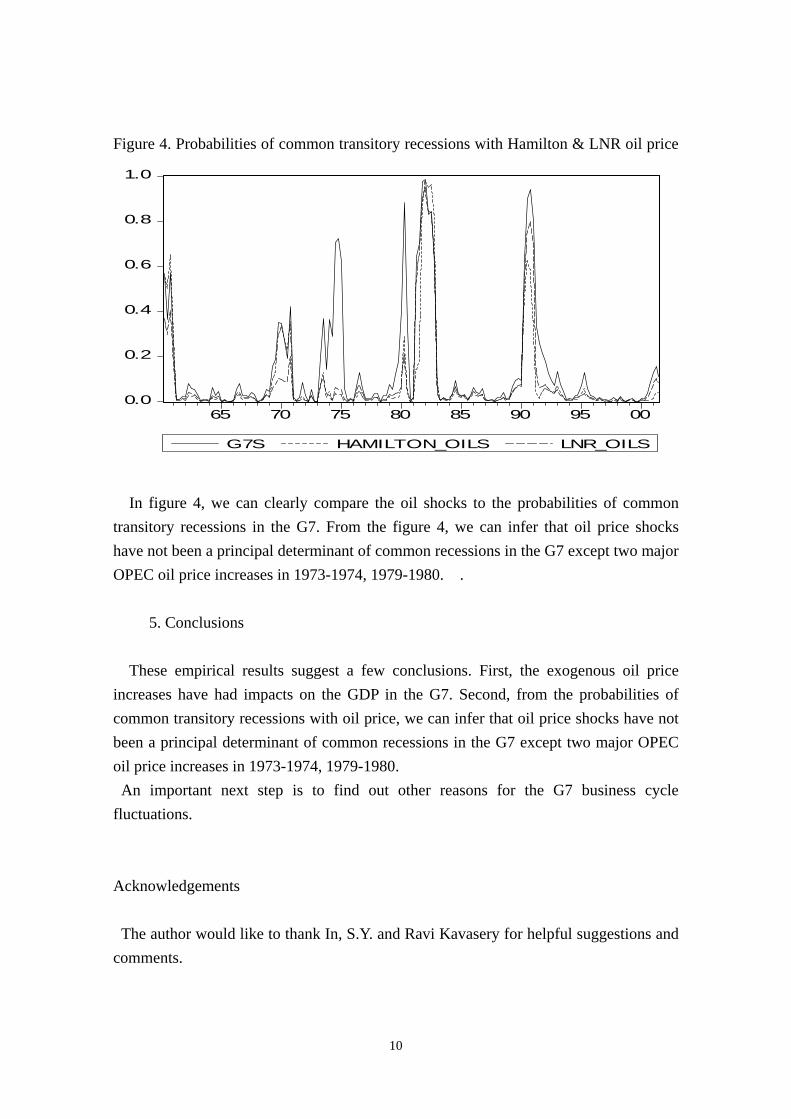
Figure 4. Probabilities of common transitory recessions with Hamilton & LNR oil price

0.0

0.2

0.4

0.6

0.8

1.0

65 70 75 80 85 90 95 00

G7S HAMILTON_OILS LNR_OILS

In figure 4, we can clearly compare the oil shocks to the probabilities of common

transitory recessions in the G7. From the figure 4, we can infer that oil price shocks have not been a principal determinant of common recessions in the G7 except two major OPEC oil price increases in 1973-1974, 1979-1980. .

5. Conclusions

These empirical results suggest a few conclusions. First, the exogenous oil price

increases have had impacts on the GDP in the G7. Second, from the probabilities of common transitory recessions with oil price, we can infer that oil price shocks have not been a principal determinant of common recessions in the G7 except two major OPEC oil price increases in 1973-1974, 1979-1980. An important next step is to find out other reasons for the G7 business cycle

fluctuations. Acknowledgements The author would like to thank In, S.Y. and Ravi Kavasery for helpful suggestions and comments.

11

Appendix A

1. Representation In this section, I discuss representation of the model presented in Section 3. I employ

the following state space representation for equations (2)-(4) assuming AR(2) dynamics for the common permanent, common transitory components, and AR(1) dynamics for idiosyncratic component. This model involves unobserved Markov-switching variable St in the transitory component and an exogenous variable. The dynamics of Friedman’s Plucking Markov Switching model with an exogenous variable can be represented in the following manner: Measurement Equation : Δyt = H ξt

Transition Equation : ξt = αSt + Fξt-1 + β Zt + Vt E(Vt Vt

’) = Q Pr(St = 0 | St-1 = 0) = q , Pr(St = 1 | St-1 = 1) = p, π≠ 0 for the πSt

where r1 0 λ1 -λ1 1 0 0 0 0 0 0

r2 0 λ2 -λ2 0 1 0 0 0 0 0 H = r3 0 λ3 -λ3 0 0 1 0 0 0 0 r4 0 λ4 -λ4 0 0 0 1 0 0 0 r5 0 λ5 -λ5 0 0 0 0 1 0 0

r6 0 λ6 -λ6 0 0 0 0 0 1 0 r7 0 λ7 -λ7 0 0 0 0 0 0 1

Δct 0 0 vt

Δct-1 0 0 0 xt π St ∑βi Zt-i ut xt-1 0 0 0

ξt = z1t αSt = 0 βZt = 0 Vt = e1t z2t 0 0 e2t z3t 0 0 e3t

z4t 0 0 e4t

z5t 0 0 e5t

z6t 0 0 e6t

z7t 0 0 e7t

12

φ1 φ2 0 0 0 0 0 0 0 0 0 1 0 0 0 0 0 0 0 0 0 0 0 0 ψ1 ψ2 0 0 0 0 0 0 0

0 0 1 0 0 0 0 0 0 0 0 F = 0 0 0 0 τ1 0 0 0 0 0 0

0 0 0 0 0 τ2 0 0 0 0 0 0 0 0 0 0 0 τ3 0 0 0 0 0 0 0 0 0 0 0 τ4 0 0 0

0 0 0 0 0 0 0 0 τ5 0 0 0 0 0 0 0 0 0 0 0 τ6 0 0 0 0 0 0 0 0 0 0 0 τ7

and

1 0 0 0 0 0 0 0 0 0 0 0 0 0 0 0 0 0 0 0 0 0 0 0 1 0 0 0 0 0 0 0 0

0 0 0 0 0 0 0 0 0 0 0 Q = 0 0 0 0 σ2

1 0 0 0 0 0 0 0 0 0 0 0 σ2

2 0 0 0 0 0 0 0 0 0 0 0 σ2

3 0 0 0 0 0 0 0 0 0 0 0 σ2

4 0 0 0 0 0 0 0 0 0 0 0 σ2

5 0 0 0 0 0 0 0 0 0 0 0 σ2

6 0 0 0 0 0 0 0 0 0 0 0 σ2

7

2. Estimation Defining St and its transitional dynamics as in equations (2)~(4), the above state-space model is an example of that considered by Kim(1994). The following describes Kim’s Markov Switching approximate maximum likelihood estimation algorithm. For details of the nature of the approximation and the Bayesian alternative to the estimation procedure, readers are referred to Kim and Nelson(1998). The above state-space model’s specific feature is that G7 real GDP’s common transitory component follows the Friedman’s plucking model by Kim and Nelson(1999), Kim and Murray (2002) . The Kim’s Markov Switching approximate maximum likelihood estimation algorithm

13

is computationally efficient, and experience suggests that the degree of approximation is small ; See Kim(1994) and Kim and Nelson(1998). Conditional on St = j and St-1 = i, the Kalman filter equations can be written as:

ξ(i,j)

t|t-1 = αSt + Fξ i

t-1|t-1 + β Zt P

(i,j)t|t-1 = F P i

t-1|t-1 F’ + Q n (i,j)t|t-1 = Δyt - Hξ(i,j)

t|t-1

f (i,j)

t|t-1 = H P (i,j) t|t-1 H’

ξ(i,j)t|t = ξ(i,j)

t|t-1 + P (i,j) t|t-1 H’[f

(i,j)t|t-1]-1 n (i,j)t|t-1

P (i,j)

t|t = (I - P (i,j) t|t-1 H’[f(i,j)

t|t-1]-1) H P (i,j) t|t-1

where Zt is an exogenous variable. ξ(i,j)

t|t-1 is an inference on ξt based on information up to time t-1, conditional on St = j and St-1 = i ; ξ(i,j)

t|t is an inference on ξt based on information up to time t, conditional on St = j and St-1 = i ; P (i,j)

t|t-1, P (i,j)

t|t

are the MSE matrices of ξ(i,j)t|t-1 and ξ(i,j)

t|t respectively; n (i,j)t|t-1 is the conditional

forecast error of Δyt based on information up to time t-1; f (i,j)t|t-1 is the conditional

variance of n (i,j)t|t-1.

As noted by Harrison and Stevens(1976) and Gordon and Smith(1988) each iteration of the Kalman filter produces a 4-fold increase in the number of cases to consider. To render the Kalman filter operational, we need to collapse the 42 posteriors (ξ(i,j)

t|t and P

(i,j)t|t ) into 4 at each iteration. Collapsing requires the following approximations

suggested by Harrison and Stevens (1976) :

Σ2i=1 Pr[St-1 = i, St = j |Ωt] ξ(i,j)

t|t ξj

t|t =

Pr[St = j |Ωt]

and Σ2

i=1 Pr[St-1 = i, St = j |Ωt] { P (i,j)

t|t+(ξjt|t -ξ(i,j)

t|t) (ξjt|t -ξ(i,j)

t|t)’} P

jt|t =

Pr[St = j |Ωt]

where Ωt refers to information available at time t. In order to obtain the probability terms necessary for collapsing, we needs the following procedure due to Hamilton(1989) :

14

Step 1 : At the beginning of the ith iteration, given Pr[St-1 = i |Ωt-1], we calculate Pr[St-1 = i, St = j |Ωt-1] = Pr[St = j | St-1 = i] Pr[St-1 = i |Ωt-1] Step 2 :

Consider the joint density of Δyt, St, and St-1 : f (Δyt , St-1 = i, St = j |Ωt-1) = f (Δyt | St-1 = i, St = j, Ωt-1) Pr[St-1 = i, St = j |Ωt-1]

from which the marginal density of Δyt is obtained by:

f (Δyt |Ωt-1) = Σ2i=1Σ

2j=1 f (Δyt , St-1 = i, St = j |Ωt-1)

= Σ2

i=1Σ2

j=1 f (Δyt | St-1 = i, St = j, Ωt-1) Pr[St-1 = i, St = j |Ωt-1]

where the conditional density f (Δyt | St-1 = i, St = j, Ωt-1) is obtained via the prediction-error decomposition:

f (Δyt | St-1 = i, St = j, Ωt-1)

= ( 2π)-T/2 | f (i,j)t|t-1|-1/2 exp{-1/2 n (i,j)’t|t-1 f (i,j)t|t-1-1 n (i,j)t|t-1}

Step 3 :

Once Δyt is observed at the end of time t, we update the probability terms: Pr[St-1 = i, St = j |Ωt] = Pr[St-1 = i, St = j |Ωt-1,Δyt ]

= f ( St-1 = i, St = j, Δyt |Ωt-1 ) f ( Δyt |Ωt-1 )

= f (Δyt | St-1 = i, St = j, Ωt-1) Pr[St-1 = i, St = j |Ωt-1 ] f ( Δyt |Ωt-1 ) with Pr[ St = j |Ωt] = Σ2

i=1 Pr[St-1 = i, St = j |Ωt] As a byproduct of the above filter in Step 2, we obtain the log likelihood function:

ln L = Σ ln(f ( Δyt |Ωt-1 )) which can be maximized with respect to the parameters of the model.

15

Appendix B

1. Summary Unit Root Tests8 for the quarterly G7 real GDP (1960:1 – 2002:4 ) ==============================================================

Augmented Dickey Fuller t-Statistic Critical Value 10% 5% 1%

============================================================== Y U.S.A -0.78 Y JAPAN -1.56 Y GERMANY -2.52

Y FRANCE -2.45 -3.14 -3.44 -4.02 Y ITALY -2.31 Y U.K -1.15 Y CANADA -1.16 ==============================================================

* reject 10% critical value, ** reject 5% critical value, *** reject 1% critical value

3. Johansen(1991, 1995) Cointegration Tests9 for the quarterly G7 real GDP ( 1960:1 – 2002:4 )

============================================================== Null Hypothesis Test Statistic Critical Value

5% 1% ============================================================== No Cointegration Vectors 125.6* 124.2 133.6 At Most One Cointegration Vectors 78.5 94.2 103.2 At Most Two Cointegration Vectors 47.3 68.5 76.1 At Most Three Cointegration Vectors 30.1 47.2 54.5 At Most Four Cointegration Vectors 15.2 29.7 35.7 At Most Five Cointegration Vectors 6.8 15.4 20.0 At Most Six Cointegration Vectors 0.0 3.8 6.7

* reject 5% critical value ** reject 1% critical value

8 4 lag was chosen for real GDP. Tests for real GDP included a time trend and constant in the test regression 8 The test statistic is the Likelihood Ratio statistic and calculated in Eviews using a lag order 4 and each series has a linear trend but the co-integration equation has only intercepts.

16

Appendix C

4. Sources for GDP Data I thank Dalsgaard, Elmeskov and Park for sending me the internal OECD series from

Dalsgaard, Elmeskov and Park(2002). In the Stock and Watson(2003) p27, Real GDP series were used for each of the G7 countries for the same period 1960:1 – 2002:4. The table below gives the data sources and sample periods for each periods for each data series used. Abbreviations used the source column are (DS) DataStream, (DRI) Data Resources and (E) for an internal OECD series from Dalsgaard, Elmeskov, and Park(2002).

==============================================================

Country Source Sample period

Canada OECD (DS) 1960:1 1960:4 STATISTICS CANADA (DS) 1961:1 2002:4

France OECD (DS) 1960:1 1977:4 I.N.S.E.E. (DS) 1978:1 2002:4

Germany DEUTSCHE BUNDESBANK (DS) 1960:1 2002:4

Italy OECD (DS) 1960:1 1969:4 ISTITUTO NAZIONALE DI STATISTICA (DS) 1970:1 2002:4

Japan OECD (DS) 1960:1 2002:4

UK OFFICE FOR NATIONAL STATISTICS (DS) 1960:1 2002:4

US Dept. of Commerce (DRI) 1960:1 2002:4

17

Figure 5. G7 real GDP : 1960:1 ~ 2002:4

2000

4000

6000

8000

10000

60 65 70 75 80 85 90 95 00

US

200000

400000

600000

800000

000000

200000

60 65 70 75 80 85 90 95 00

CANADA

40000

80000

120000

160000

200000

240000

60 65 70 75 80 85 90 95 00

UK

50000

100000

150000

200000

250000

300000

350000

400000

60 65 70 75 80 85 90 95 00

FRANCE

100

200

300

400

500

600

60 65 70 75 80 85 90 95 00

GERMANY

50000

100000

150000

200000

250000

300000

60 65 70 75 80 85 90 95 00

ITALY

0

20

40

60

80

100

120

60 65 70 75 80 85 90 95 00

JAPAN

18

Figure 6. G7 log differenced real GDP from 1960:2 ~ 2002:4

-8

-4

0

4

8

12

65 70 75 80 85 90 95 00

USJAPANGERMANY

FRANCEIT ALYUK

CANADA

19

References Beaudry, Paul, Gary Koop (1993) Do recessions permanently change output? Journal of Monetary Economics 31:149-163 Box and Jenkins (1976) Time Series Analysis : forecasting and control , Holden Day. Campbell, John Y., Mankiw, N. G.. (1987) Are out fluctuations transitory ? Quarterly Journal of Economics 102:857-880 Chauvet, M. (1998) An econometric characterization of business cycle dynamics with factor structure and regime switching. International Economic Review 39:969-996 Clark, Peter K. (1987) The cyclical component of U.S. economic activity. Quarterly Journal of Economics 102:797-814 Clements, M. P., Krolzig, H.-M. (2002) Can oil shocks explain asymmetries in the US Business Cycle? Empirical Economics 27:185-204 Cohrane, John H. (1988) How big is the random walk in GNP? Journal of Political Economy 96:893-923. Dalsgaard, T., Elmeskov, J., Park, C.Y.(2002) Ongoing Changes in the Business Cycle - Evidence and Causes. OECD Economic Department Working Paper 315 Gregory, Allan W & Head, Allen C & Raynauld, Jacques (1997) Measuring World Business Cycles. International Economic Review 38:677-701. Hamilton, J.D.(1983) Oil and the Macroeconomy since World War II. Journal of Political Economy 91:228-248 Hamilton, J.D.(1989) A new approach to the economic analysis of nonstationary time series and the business cycle. Econometrica 57:357-384 Hamilton, J.D.(1996) This is what happened to the oil price-macroeconomy relationship. Journal of Monetary Economics 38:215-220 Hamilton, J.D.(1994) Time series analysis. Princeton University Press, Princeton Hamilton, J.D.(2003) What is an oil shock? Journal of Econometrics 113:363-398 Hooker, M. A. (1996) Whatever happened to the oil price-macroeconomy relationship? Journal of Monetary Economics 38:195-213 Hooker, M. A. (1996) This is what happened to the oil price-macroeconomy relationship: Reply. Journal of Monetary Economics 38:221-222 Kim, C.J. (1994) Dynamic factor models with Markov switching. Journal of Econometrics 60:1-22 Kim, C.J., Nelson, C.R. (1998) Business cycle turning points. A new coincident index and tests of durations dependence based on a dynamic factor model with regime switching. Review of Economics and Statistics 80:188-201

20

Kim, C.J., Nelson, C.R. (1999) State-space models with regime switching: Classical and Gibbs sampling approaches with applications. MIT Press, Cambridge Kim, C.J., Nelson, C.R.(1999) Friedman’s Plucking Model of Business Fluctuations: Tests and Estimates of Permanent and Transitory Component. Journal of Money, Credit, and Banking 31:317-334 Kim, C.J., Murray, C.J.(2002) Permanent and transitory components of recessions. Empirical Economics 27:163-183 Kim, C.J, Piger J., Startz, R. (2002) Permanent and Transitory Components of Business Cycles: Their Relative Importance and Dynamic Relationship. The Federal Reserve Bank of St. Louis Working Paper 2001-017B Kose, M.A., Otrok ,C., Whiteman, C.H. (2002) Understanding the Evolution of World Business Cycles. presentation. Kose, M.A., Otrok, C., Whiteman, C.H. (2003) International Business Cycles: World, Region, and Country-Specific Factors. Forthcoming, American Economic Review Lam, Pok Sang (1990) The Hamilton model with a general autoregressive component: estimation and comparison with other models of economic time series. Journal of Monetary Economics 26:409-432 Lee, K., Ni, S., Ratti, A.(1995) Oil shocks and the macroeconomy: The role of price variability. Energy Journal 16:39-56 Monfort A., J.P.Renne, R. Ruffer, G.. Vitale (2002) Is Economic Activity in the G7 Synchronized? Common Shocks vs. Spillover Effects. CEPR Discussion Paper No. 4119 Mork, K. A. (1989) Oil and the Macroeconomy when prices go up and down: An extension of Hamilton’s results. Journal of Political Economy 97:703-708 Nelson, Charles R., Plosser, Charles I., (1982) Trends and random walks in macroeconomic time series: Some evidence and implications. Journal of Monetary Economics 10:139-162 Rasche, R.H., Tatom, J.A. (1977) Energy resources and potential GNP. Federal Reserve Bank of St. Louis Review 59:10-24 Rasche, R.H., Tatom, J.A. (1981) Energy price shocks, aggregate supply, and monetary policy: the theory and international evidence. In: Brunner, K., Meltzer, A. H. (eds.), Supply Shocks, Incentives, and National Wealth, Carnegie-Rochester Conference Series on Public Policy, Vol. 14 North Holland, Amsterdam. Raymond, J. E., Rich, R. W. (1997) Oil and the macroeconomy: A Markov state-switching approach. Journal of Money, Credit, and Banking 29:193-213 Stock, J.H., Watson, M.W. (1989) New indexes of coincident and leading indicators. In:

21

Blanchard OJ, Fisher S. (eds) NBER macroeconomics annual. MIT Press, pp351-393 Stock, J.H., Watson, M.W. (1991) A probability model of the coincident and leading indicators. In: Lahiri K, Moore GH(eds.) Leading economic indicators: New approaches and forecasting records. Cambridge University Press, New York, pp63-85 Stock, J.H., Watson, M.W.(2003) Understanding changes in international business cycle dynamics. NBER working paper 9859 Tatom, John A. (1988) Are the macroeconomic effects of oil price changes symmetric? In: Karl Brunner and Allan H. Meltzer(eds.) Stabilization policies and labor markets: Carnegie-Rochester Conferences on Public Policy 28:325-368. Amsterdam, North Holland Watson, Mark M. (1986) Univariate detrending methods with stochastic trends. Journal of Monetary Economics 18:29-75 Yoon, Jae Ho (2004) Has the G7 business cycle become more synchronized? POSCO Research Institute Working Paper 2004