ohio state - eurecom · phil schniter the ohio state university ... freq selective) chans. some...
TRANSCRIPT

Phil Schniter The Ohio State University'
&
$
%
Efficient Multi-Carrier Communication
over Mobile Wideband Channels
Phil Schniter
OHIOSTATE
T . H . E
UNIVERSITY
July 2008(Joint work with Mr. Sungjun Hwang and Dr. Sib Das)
1

Phil Schniter The Ohio State University'
&
$
%
Multipath, Mobility, and Bandwidth:
Trends:
• As the signal bandwidth increases, there are more gain variations across
the signal bandwidth, and hence more channel parameters.
Increased BW ⇒ longer channel impulse response.
• As the mobilities of the transmitter, receiver, and reflectors increase,
there are more channel gain variations per unit time.
Increased mobility ⇒ faster impulse response variation.
2

Phil Schniter The Ohio State University'
&
$
%
Multipath Fading (cont.):
• Implication:
As bandwidth & mobility increase, time-domain receivers need to
implement longer filters and adapt them at faster rates.
• Example — North American Digital TV:
Typical receivers use decision feedback equalization (DFE) with 1000
taps in the feedforward path and 500 in the feedback path.
+FF
FB
decisions
DFE
Even with a fixed transmitter and receiver, it is very difficult to adapt
such long filters quickly enough!
3

Phil Schniter The Ohio State University'
&
$
%
Orthogonal Frequency Division Multiplexing (OFDM):
Main Ideas:
1. Transmit data in parallel over non-interfering narrowband subchannels.
• Flat frequency response across each subchannel ⇒ 1 channel coefficientsubchannel
.
• Equalization = one complex gain adjustment per subchannel!
2. Implement subchannelization using the Fast Fourier Transform (FFT).
• No calibration or drift issues like with analog modulators.
• Minimal frequency spacing (⇒ good spectral efficiency).
• Fast implementation: N log2 N multiplications per N -FFT.
• Requires a guard interval of length-L−1.
time? ?? ?
L−1L−1 L−1L−1 NNN
4

Phil Schniter The Ohio State University'
&
$
%
Equalization Complexity:
Single-carrier:
.+
3L
2L
L
decisions
decisions
Viterbi
DFE:
Linear:
MLSD:
3L mults per QAM symbol
3L mults per QAM symbol
|S|L mults per QAM symbol
Complexity scales linearly or exponentially in the channel length L.
Multi carrier:
N + N log2 N mults per block, where typically N ≈ 4L.
⇒ 1 + log2 N = 3 + log2 L mults per QAM symbol.
Complexity scales logarithmically in the channel length L.
Example: When L = 512, we have 3L = 1536 and 3 + log2 L = 12.
5

Phil Schniter The Ohio State University'
&
$
%
CP-OFDM:
Principal advantage:
• Low-complexity demod with delay-spreading (i.e., freq selective) chans.
Some disadvantages:
• Sensitive to Doppler-spreading (i.e., time selective) channels.
• Loss of spectral efficiency due to the insertion of guards.
What if we increased N relative to L (i.e., P , NL≫ 4)?
– Complexity increases to 1 + log2 P + log2 L multsQAM symbol
...not bad.
– Reduced subcarrier spacing ⇒ more sensitive to Doppler spread!
• Slow spectral roll-off causes interference to adjacent-band systems.
Improves with raised-cosine pulse, but at further loss in efficiency:
timeL−1 L−1L−1 N N N
• High peak-to-average power ratio (PAPR).
6

Phil Schniter The Ohio State University'
&
$
%
The Big Question:
Can we fix CP-OFDM’s
• sensitivity to Doppler spread
• loss in spectral efficiency, and
• slow spectral roll-off,
without spoiling its O(log2 L) multsQAM symbol
complexity scaling?
7

Phil Schniter The Ohio State University'
&
$
%
The Big Question:
Can we fix CP-OFDM’s
• sensitivity to Doppler spread
• loss in spectral efficiency, and
• slow spectral roll-off,
without spoiling its O(log2 L) multsQAM symbol
complexity scaling?
Yes!
Re-think the role of “pulse shaping” in multi-carrier modulation. . .
8

Phil Schniter The Ohio State University'
&
$
%
Rectangular Pulses:
A standard CP-OFDM block can be recognized as a sum of N infinite-length
complex exponentials windowed by a rectangular pulse of width N+L−1.
=+
+
t
t
t
tN+L−1
N+L−1
N+L−1
N+L−1N+L−1N+L−1
⇒ Dirichlet sinc in DTFT domain, whose slow side-lobe decay causes:
• strong interference to adjacent-band communication systems, and
• high sensitivity to Doppler spreading:
Doppler(ejω) |Dsinc(ejω)|2
∗
−fD fD −2π . . . . . . . . . . . . −4πN
−2πN
0 2πN
4πN
. . .. . . . . .. . . 2π
9

Phil Schniter The Ohio State University'
&
$
%
Smooth Overlapping Pulses:
What if we applied a smooth window instead?
=+
+
t
t
t
t Ns
Ns
NsNs
The main-lobe is wider but the sidelobes decay more quickly, implying:
• reduced adjacent-band interference, and
• strong interference from adjacent subcarriers, but very little interference
from all other subcarriers, even under large Doppler spreads:
Doppler(ejω) |A(ejω)|2
∗
−fD fD −2π . . . . . . . . . . . . −4πN
−2πN
0 2πN
4πN
. . .. . .. . . . . . 2π
10

Phil Schniter The Ohio State University'
&
$
%
Smooth Overlapping Pulses:
Challenge: The use of smooth overlapping pulses potentially causes
inter-carrier interference (ICI) and inter-block interference (IBI):
x(i) =∞∑
q=−∞
H(i, q)︸ ︷︷ ︸
subcarriercoupling matrix
s(i − q) + z(i). Difficult to equalize!
Solution: Design the pulse shapes with the goal of. . .
1. Completely suppressing IBI: H(i, q)∣∣q 6=0
= 0.
2. Allowing ICI only within a radius of D ≪ N subcarriers. (Often D = 1.)
= + Not difficult to equalize.D
x(i) H(i, 0) s(i) z(i)
11

Phil Schniter The Ohio State University'
&
$
%
Receiver Pulse-Shaping:
Though so far we’ve considered a non-rectangular transmission pulse {an},
tn =∞∑
i=−∞
an−iNs
N−1∑
k=0
sk(i)ej 2π
Nkn, n = −∞ . . .∞,
we can use, in addition, a non-rectangular reception pulse {bn}:
xk(i) =∞∑
n=−∞
rn−iNsbn e−j 2π
Nkn, k = 0 . . . N − 1.
Ns specifies the interval between the start of one OFDM block and the next.
• Modulation efficiency η , NNs
symbols
sec Hz
• For OFDM, Ns = N+L−1, but now there is no constraint on Ns!
We focus on Ns = N ⇔ no guard interval ⇔ η = 1.
12

Phil Schniter The Ohio State University'
&
$
%
Max-SINR Pulse Design:
Writing the received signal energy components due to
Es =∑
(q,k,l)∈¥
E{|Hk,l(·, q)|2} “signal” and
Ei =∑
(q,k,l)∈¥
E{|Hk,l(·, q)|2} “interference” (IBI+ICI)
· · ·· · ·interferencedon’t caresignal
where {H(·, q)} =
we can write SINR =Es
Ei + En
=aHP 1(b)a
aHP 2(b)a=
bHP 3(a)b
bHP 4(a)bwhere
a = transmission pulse coefficientsb = reception pulse coefficients
P 1(·),P 2(·),P 3(·),P 4(·) = matrix fxns dependant on Doppler & SNR.
⇒ SINR-maximizing pulses are generalized eigenvectors.
13

Phil Schniter The Ohio State University'
&
$
%
Max-SINR Pulse Examples:
0 100 200 300
0
0.5
1
1.5
TxRx
0 100 200 300 400 500
0
0.5
1
1.5
0 100 200 300 400 500
0
0.5
1
1.5
0 100 200 300 400 500
0
0.5
1
1.5
ZP-OFDM (η = 0.803) Optimized receiver (η = 1)
Optimized transmitter (η = 1) Jointly optimized (η = 1)
14

Phil Schniter The Ohio State University'
&
$
%
IBI/ICI Energy Profiles (same for each subcarrier):
0 5 10 15−100
−90
−80
−70
−60
−50
−40
−30
−20
−10
0
10
0 5 10 15−100
−90
−80
−70
−60
−50
−40
−30
−20
−10
0
10
0 5 10 15−100
−90
−80
−70
−60
−50
−40
−30
−20
−10
0
10CP−OFDM η=0.803
ZP−OFDM η=0.803
ROMS η=1
TOMS η=1
JOMS η=1
previous block same block next block
dB
subcarrier separationsubcarrier separationsubcarrier separation
D = 1, SNR = 15dB, L = 64, fDTc = 7.6× 10⁻⁴, Jakes Doppler spectrum.
(For example, fc = 20GHz, BW=3MHz, Th = 5.4µs, v = 120km/hr.)
15
Phil Schniter The Ohio State University'
&
$
%
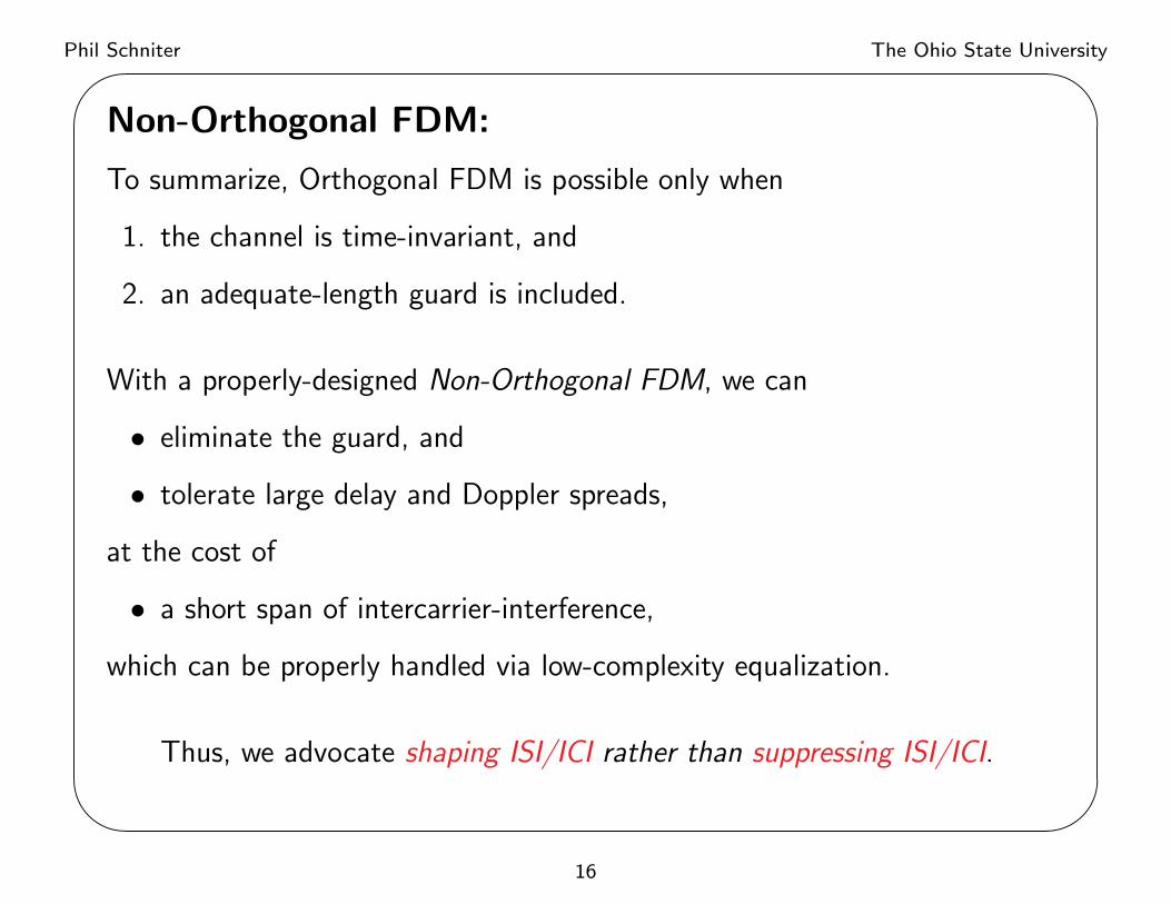
Non-Orthogonal FDM:
To summarize, Orthogonal FDM is possible only when
1. the channel is time-invariant, and
2. an adequate-length guard is included.
With a properly-designed Non-Orthogonal FDM, we can
• eliminate the guard, and
• tolerate large delay and Doppler spreads,
at the cost of
• a short span of intercarrier-interference,
which can be properly handled via low-complexity equalization.
Thus, we advocate shaping ISI/ICI rather than suppressing ISI/ICI.
16

Phil Schniter The Ohio State University'
&
$
%
Outage Capacity vs NfDTs for various ICI-radii D:
0 0.5 1 1.5 2 2.5 3 3.5 4 4.5 5
1.4
1.6
1.8
2
2.2
2.4
2.6
0.00
01−
outa
ge c
apac
ity [b
its/u
se]
GP−FDMN=16M=4Nh=8Ng=0
SNR=10
D=0D=1D=2D=3D=4D=5
NfDTs
• The outage-capacity optimal D obeys D ≈ ⌊NfDTs⌉!
• ICI shaping is better than ICI suppression when 2fDTs ≥1N
.
17

Phil Schniter The Ohio State University'
&
$
%
ICI Equalization:
Coherent approaches (i.e., known channel): multsQAM symbol
1. Viterbi [Matheus/Kammeyer GLOBE 97] O(|S|DD)
2. Iterative Soft [Das/Schniter Asilomar 04] O(D2)
3. Linear MMSE [Rugini/Banelli/Leus SPL 05] O(D2)
4. MMSE DFE [Rugini/Banelli/Leus SPAWC 05] O(D2)
5. Tree Search [Hwang/Schniter SPAWC 06] O(D2)
Non-coherent approaches (i.e., unknown channel):
1. Hard Tree Search [Hwang/Schniter WUWNet 07] O(D2L2)
2. Soft Tree Search [Hwang/Schniter Asilomar 07] O(D2L2)
18

Phil Schniter The Ohio State University'
&
$
%
1) Coherent Tree Search:
Two-step procedure:
1. MMSE-GDFE pre-processing [Damen/ElGamal/Caire TIT 03]:
DD + 1 2D + 1 2D
N
à O(D2N) algorithm [Rugini/Banelli/Leus SPAWC 05].
2. Near-optimal yet efficient tree search. Options include:
• Depth-first search (e.g., Schnor-Euchner sphere decoder),
• Best-first search (e.g., Fano alg, stack alg),
• Breadth-first search (e.g., M-alg, T-alg, Pohst sphere decoder).
19

Phil Schniter The Ohio State University'
&
$
%
Performance:
10 15 20 2510
−4
10−3
10−2
10−1
100
SNR in dB
fram
e er
ror
rate
DFEFanoM−algT−algadaptive T−algSE−SpDML
10 15 20 2510
−4
10−3
10−2
10−1
100
SNR in dB
fram
e er
ror
rate
DFEFanoM−algT−algadaptive T−algSE−SpDML
fDTc = 0.001 fDTc = 0.003
Suboptimal tree search is almost indistinguishable from ML!
20

Phil Schniter The Ohio State University'
&
$
%
Average Complexity (MACs/frame):
10 15 20 25 302.2
2.4
2.6
2.8
3
3.2
3.4
SNR in dB
log
(ope
ratio
ns)
Viterbi
Fano
SE−SpD
M−alg
T−alg
Adaptive T−alg
DFE
10 15 20 25 302.2
2.4
2.6
2.8
3
3.2
3.4
SNR in dB
log
(ope
ratio
ns)
Viterbi
Fano
SE−SpD
M−alg
T−alg
Adaptive T−alg
DFE
fDTc = 0.001 fDTc = 0.003
NN
Breadth-first & DFE stay cheap, while depth-first & Fano explode!
21

Phil Schniter The Ohio State University'
&
$
%
Error Masking due to V-shaped Channel Matrix:
After MMSE-GDFE pre-processing, we get the following system:
= +
0 2D + 1 2D
N − 2D − 1N − 2D − 1N − 4D − 2
Key point: The blue symbol does not affect any of the red observations.
Error-masking explains the complexity explosion of the depth-first
and Fano searches!
22

Phil Schniter The Ohio State University'
&
$
%
2) Iterative Soft ICI Cancellation:
+=
xk
Hk
hksk
sk
zk
xk = Hksk + zk
• Soft interference cancellation using mean of sk.
• Assuming Gaussian residual interference and us-
ing the covariance of sk, compute LLRs(sk).
• Using LLRs(sk), update mean/covariance of sk.
• k → 〈k + 1〉N .
23

Phil Schniter The Ohio State University'
&
$
%
Iterative Soft ICI Cancellation (BPSK example):
updatepriors SIC
updateLLR
LLR(i)k
s(i)k , v
(i)k g
(i)k LLR
(i+1)k
s(i)k , E{sk|sk} = tanh(LLR
(i)k /2)
v(i)k , var(sk|sk) = 1 − (s
(i)k )2
y(i)k = xk − Hks
(i)k
g(i)k = y
(i)Hk
(Rz + Hk D(v
(i)k )HH
k
)−1hk
LLR(i+1)k = LLR
(i)k + 2 Re(g
(i)k )
Complexity: Miters
× O(D2)mtx inv
per BPSK symbol.
24
Phil Schniter The Ohio State University'
&
$
%
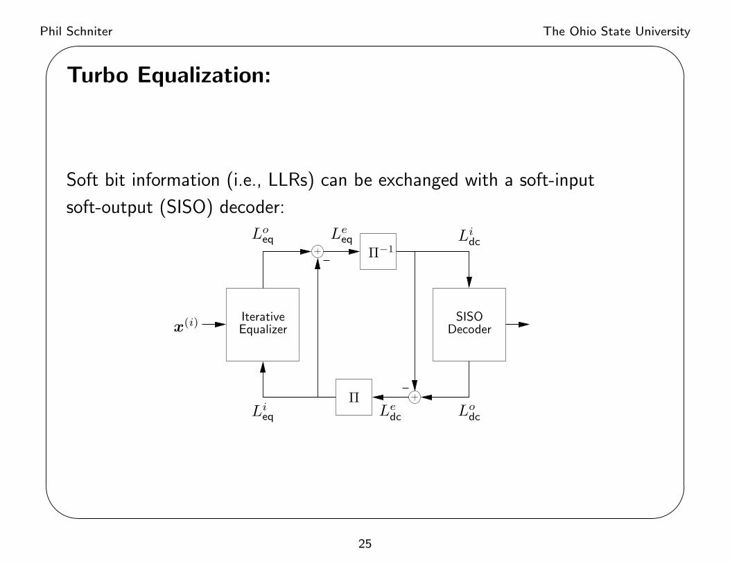
Turbo Equalization:
Soft bit information (i.e., LLRs) can be exchanged with a soft-input
soft-output (SISO) decoder:
x(i) IterativeEqualizer
Lo
eq
Li
eq
Le
eq Li
dc
Le
dc Lo
dc
Π−1
Π
SISODecoder
25

Phil Schniter The Ohio State University'
&
$
%
Turbo Equalization Performance:
0 5 10
10−4
10−3
10−2
10−1
Eb/N
o (dB)
BE
R
0 5 10
10−4
10−3
10−2
10−1
Eb/N
o (dB)
0 5 10
10−4
10−3
10−2
10−1
Eb/N
o (dB)
LINML1MS1MS8ML8PLICPGIC
LINML1MS1MS8ML8PLICPGIC
LINML1MS1MS8ML8PLICPGIC
TOMS JOMS ROMS rate-12
conv code
QPSK
N = 64
D = 2
L = 16
fDTc = 0.003
for example:
fc = 20GHz
BW= 3MHz
Th = 5.4µs
v = 3×160km/hr
26

Phil Schniter The Ohio State University'
&
$
%
3) Non-Coherent Equalization:
• So far we have assumed that the equalizer is provided with channel
estimates.
But with long and quickly varying channels, accurate channel
estimation requires a high proportion of pilots!
• Instead, one might consider joint estimation of channel and symbols.
Actually, we are not interested in explicitly estimating the channel,
but rather doing non-coherent equalization: inferring transmitted
bits using knowledge of channel statistics but not channel state.
For this it helps to re-parameterize the system model. . .
27

Phil Schniter The Ohio State University'
&
$
%
Basis-Expansion Model:
From the pulse-shaped FDM model:
x(n) = H(n)s(n) + z(n) H(n) is banded with band radius D
= S(n)h(n) + z(n) h(n) ∈ C(2D+1)N ICI coefs
we can use a basis-expansion model (BEM) for the ICI coefs:
h(n) = Bθ(n) θ(n) ∈ C(2D+1)L delay/Doppler coefs
B =
(FL ...
FL
)
F L ∈ CN×L truncated DFT matrix
to rewrite the observation as
x(n) = S(n)Bθ(n) + z(n).
Note: if we knew the locations of K active sparse taps, we would only
include those columns of the DFT matrix, giving θ(n) ∈ C(2D+1)K .
28

Phil Schniter The Ohio State University'
&
$
%
Non-coherent MLSD:
Treating the delay/Doppler coefs θ as nuisance parameters,
sML = arg maxs
p(x|s)
= arg maxs
∫
θ
p(x|s, θ)p(θ)dθ
Assuming θ ∼ CN (0, Rθ),
sML = arg maxs
{xHSBΣ
−1s
BHSHx − σ2 log |Σs|}
Σs , BHSHSB + σ2R−1θ
Since θMMSE|s = Σ−1s
BHSHx, we can rewrite
sML = arg maxs
{
‖x − SBθMMSE|s‖2 − σ2 log |Σs|
}
But how do we avoid an exhaustive search over s?
29

Phil Schniter The Ohio State University'
&
$
%
Fast Tree Search:
By turning off the first and last D subcarri-
ers, H becomes upper-triangular, facilitat-
ing the use of tree-search.
= +
x H s w
s0 = [s0]T
s1 = [s0, s1]T
s2 = [s0, s1, s2]T
s3 = [s0, s1, s2, s3]T
(for BPSK)
The important thing here is that the partial ML metric
µML(sk) = ‖xk − SkBkθMMSE|sk‖2 − σ2 log |Σk|
can be computed recursively. Thus, total search complexity via the
M -algorithm is only
2M |S|(2D + 1)2L2 mults per QAM-symbol!
30

Phil Schniter The Ohio State University'
&
$
%
Complexity Reduction via Pilots:
• With non-coherent decoding, we require only a single pilot subcarrier.
• But, with more pilots, the initial channel estimate θMMSE improves,
allowing more aggressive branch pruning in the tree search.
Example: M-algorithm
(BPSK, 25% pilots,
M=8) compared to
coherent MLSD with
genie-aided θMMSE:
5 10 15 20 25 30
10−5
10−4
10−3
10−2
10−1
100
BE
R
SNR (dB)
joint est/det
genie-chan+MLSD
joint est/det, genie-sparse
genie-chan+MLSD, genie-sparse
31

Phil Schniter The Ohio State University'
&
$
%
Non-coherent Turbo Equalization:
softnon-coherent
equalizer
softdecoder
Π
Π−1
pilots
xbits {bk}
QN−1k=0
{Le(bk|x)}QN−1k=0
{La(bk)}QN−1k=0
Le(bk|x) = ln
∑
s: bk=1 exp µMAP(s)∑
s: bk=0 exp µMAP(s)− La(bk) ”extrinsic LLR”
µMAP(s) = ln p(x|s
)+
∑
k: bk=1
La(bk) ”MAP metric”
Need O(2QN) evaluations of µ(s) Ã Computationally infeasible!
32

Phil Schniter The Ohio State University'
&
$
%
Simplified LLR Evaluation:
The “max-log” approximation:
Le(bk|x) ≈ maxs∈L∩{s:bk=1}
µMAP(s) − maxs∈L∩{s:bk=0}
µMAP(s) − La(bk)
L : set containing the M most probable s,
requires only a few evaluations of µMAP(s).
To find L, the set of most probable s, and the MAP metrics {µMAP(s)}s∈L,
we use a tree search, as in the uncoded case.
Here again, there exists a fast metric update such that the total search
complexity, with the M-algorithm, is only
2M |S|(2D+1)2L2 mults per QAM-symbol!
33

Phil Schniter The Ohio State University'
&
$
%
Non-coherent Turbo Performance:
4 6 8 10 12 1410
−5
10−4
10−3
10−2
10−1
Eb/No(dB)
BE
R
Soft Kalman Estim Np=9Kalman−LVA Np=9NC (Proposed) Np=9Genie−Estim CHPerfect CH Knowledge rate-1
2LDPC
QPSK
N = 64
D = 2
L = 16
K = 3
fDTc = 0.003
34
Phil Schniter The Ohio State University'
&
$
%
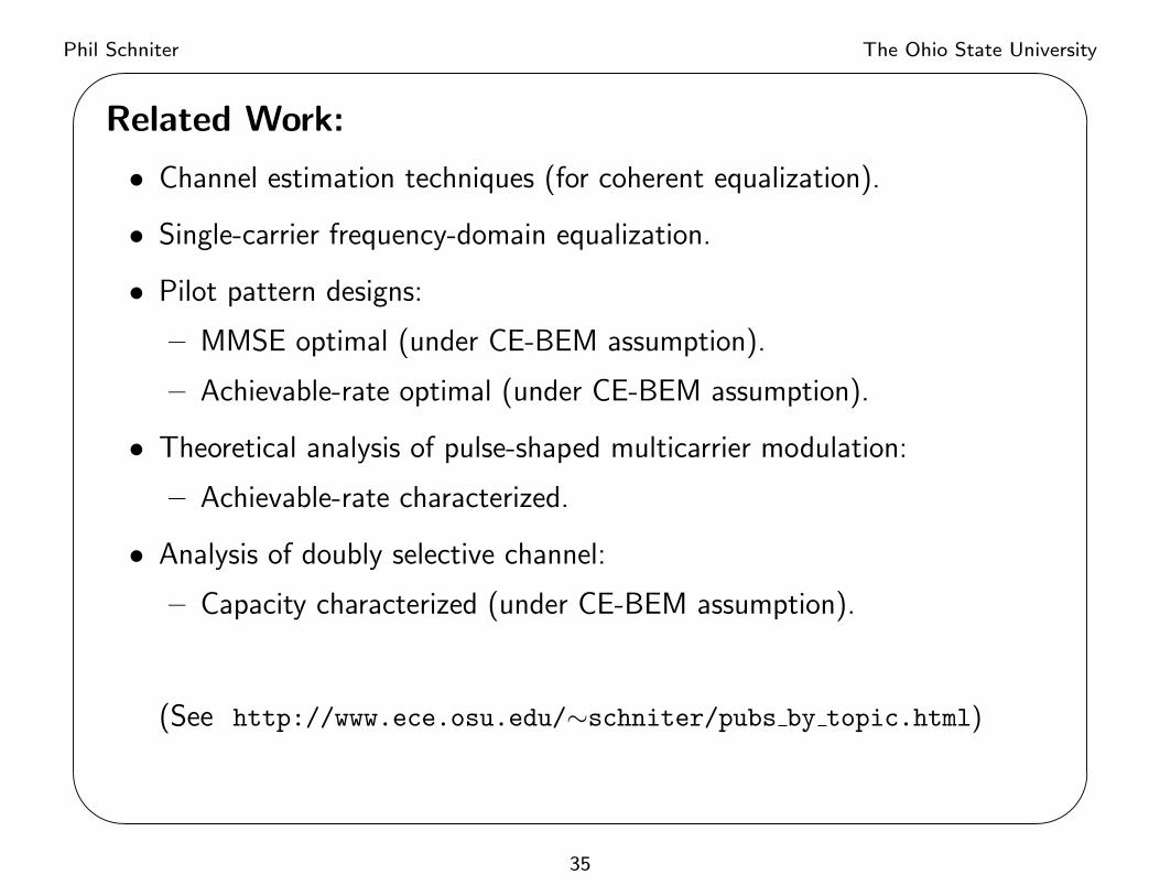
Related Work:
• Channel estimation techniques (for coherent equalization).
• Single-carrier frequency-domain equalization.
• Pilot pattern designs:
– MMSE optimal (under CE-BEM assumption).
– Achievable-rate optimal (under CE-BEM assumption).
• Theoretical analysis of pulse-shaped multicarrier modulation:
– Achievable-rate characterized.
• Analysis of doubly selective channel:
– Capacity characterized (under CE-BEM assumption).
(See http://www.ece.osu.edu/∼schniter/pubs by topic.html)
35

Phil Schniter The Ohio State University'
&
$
%
Conclusions:
Single Carrier:
• O(L) multsQAM symbol
equalization of delay-spread channels.
• Challenging to track quickly time-varying channels.
Orthogonal FDM:
• O(log2 L) multsQAM symbol
equalization of delay-spread channels.
• Loss in spectral efficiency due to guard interval.
• Sensitive to Doppler spread.
• Slow spectral roll-off ⇒ high adjacent-band interference.
Non-Orthogonal FDM:
• No need for a guard interval; high spectral efficiency.
• Large simultaneous delay & Doppler spreads ⇒ no IBI and short ICI.
• Fast spectral roll-off ⇒ low adjacent-band interference.
36

Phil Schniter The Ohio State University'
&
$
%
Equalization/Decoding of Short ICI Span:
• Uncoded Coherent:
Tree search gives ML-like performance with DFE-like complexity.
• Coded Coherent:
Iterative soft ICI cancellation in turbo configuration performs close to
perfect-interference-cancellation bound.
• Uncoded Non-Coherent:
Tree-search with fast metric update gives ML-like performance with
O(D2L2) complexity.
• Coded Non-Coherent:
Tree-search with fast metric update performs close to genie-aided bound
with O(D2L2) complexity, or O(D2K2) if sparseness leveraged.
37

Phil Schniter The Ohio State University'
&
$
%
Thanks for listening!
38