ohio higher education funding commission - ohio shared services

70 VOLUME 58J O U R N A L O F T H E A T M O S P H E R I C S C I E N C E S

q 2001 American Meteorological Society

Numerical and Laboratory Study of a Horizontally Evolving Convective BoundaryLayer. Part I: Transition Regimes and Development of the Mixed Layer

E. FEDOROVICH

Institute for Hydromechanics, University of Karlsruhe, Karlsruhe, Germany

F. T. M. NIEUWSTADT

J. M. Burgers Centre for Fluid Mechanics, Delft University of Technology, Delft, Netherlands

R. KAISER

Zeuna Starker GmbH and Company, KG, Augsburg, Germany

(Manuscript received 7 July 1999, in final form 26 April 2000)

ABSTRACT

Results are presented from a large eddy simulation (LES) and wind tunnel study of the turbulence regime ina horizontally evolving sheared atmospheric convective boundary layer (CBL) capped by a temperature inversion.The wind tunnel part of the study has been conducted in the thermally stratified tunnel of the University ofKarlsruhe. For the numerical part a modified LES procedure that was originally designed for simulation of thehorizontally homogeneous atmospheric CBL has been employed.

The study focuses on the transition between the neutrally buoyant boundary layer in the initial portion of thewind tunnel flow and a quasi-homogeneous convectively mixed layer developing downwind. The character ofthe transition between the two boundary layers and the associated changes in the turbulence structure are foundto be strongly dependent on the magnitude and distribution of disturbances in the flow at the entrance of thewind tunnel test section. For all simulated inflow conditions, the transition is preceded by accumulation ofpotential energy in the premixed CBL. The eventual energy release in the transition zone leads to turbulenceenhancement that has a form of turbulence outbreak for particular flow configurations.

The numerically simulated CBL case with temperature fluctuations introduced in the lower portion of theincoming flow appears to be the closest to the basic CBL flow case studied in the wind tunnel. Second-orderturbulence statistics derived from the LES are shown to be in good agreement with the wind tunnel measurements.Main features of transition, including the turbulence enhancement within the transition zone, are successfullyreproduced by the LES.

1. Introduction

A buoyancy driven convective boundary layer (CBL)heated from below and capped by a density interface(the so-called inversion layer) is commonly observed inthe atmosphere during daytime conditions. In the ab-sence of mean wind (the case of shear-free convection),turbulence in the CBL is solely maintained by buoyancyproduction at the heated underlying surface. The buoy-ant forcing favors vertical motions and leads to the char-acteristic cellular convection pattern composed of warmupdrafts (thermals) and associated cool downdrafts. Inthe presence of mean wind, the CBL turbulence regime

Corresponding author address: Dr. Evgeni Fedorovich, School ofMeteorology, University of Oklahoma, Energy Center, 100 East Boyd,Norman, OK 73019-1013.E-mail: [email protected]

is modified by flow shears at the surface and across theinversion layer at the CBL top.

Most numerical and laboratory studies carried out sofar have assumed statistical quasi homogeneity of theCBL over a horizontal plane and regarded the CBLevolution as a nonstationary (or nonsteady) process.Available measurement data on the convective turbu-lence structure in the atmosphere usually also refer tothis CBL type. Another type of the atmospheric CBLis the horizontally evolving CBL, which grows in aneutrally or stably stratified air mass that is advectedover a heated underlying surface. Properties of turbu-lence in this type of the CBL are much less knowncompared to the nonstationary, horizontally homoge-neous CBL case.

A thermally stratified wind tunnel was constructed atthe University of Karlsruhe (UniKa) by Rau and Plate(1995) to study the quasi-stationary, horizontally evolv-ing CBL. A series of experiments has been carried out

1 JANUARY 2001 71F E D O R O V I C H E T A L .

FIG. 1. Sketch of simulation domain (the wind tunnel test section) with the evolving CBL.

in this tunnel during the last several years aimed at acomprehensive investigation of the turbulence structurein the sheared CBL. Results of these experiments havebeen reported in Fedorovich et al. (1996), Kaiser andFedorovich (1998), and Fedorovich and Kaiser (1998).The experiments have shown that wind shears can sub-stantially modify the CBL turbulence dynamics. Thebuoyancy appeared to be the dominant mechanism ofturbulence production at larger scales of motion, whilethe role of shear was increasing toward the range ofsmaller scales. Measurements in the tunnel also gave anindication that wind shear across the inversion layer canattenuate the entrainment process and thus affect theCBL growth.

In the course of the aforementioned experiments itbecame clear that laboratory measurements should becomplemented with numerical simulations in order tobetter understand and quantitatively describe the evo-lution of turbulence regime in the horizontally inho-mogeneous CBL. Such a combination of physical ex-periment and numerical simulation was the main guid-ing idea of the present study. A similar combined ap-proach has been recently applied in the CBL studies ofOhya et al. (1998) and Ohya and Uchida (1999).

Large eddy simulation (LES), which is used as nu-merical technique in our study, has been extensivelyemployed in the atmospheric research to reproduce var-ious cases of the nonsteady, horizontally homogeneousCBL. Among the most well-known LES codes designedfor this purpose are those of Deardorff (1972), Moeng(1984), Wyngaard and Brost (1984), Nieuwstadt andBrost (1986), Mason (1989), and Schmidt and Schu-mann (1989). These codes are based on the same prog-nostic equations but use different numerical algorithmsand parameterizations of subgrid turbulence. The com-parative study of the four representative atmosphericLES codes by Nieuwstadt et al. (1993) has demonstratedthat results of their predictions are consistent with eachother, at least for the CBL cases with dominant buoyantforcing.

For the present study, the LES code described byNieuwstadt and Brost (1986) and Nieuwstadt (1990) hasbeen modified in order to allow the simulation of aspatially evolving CBL. The modified LES procedureis described in section 2 of this paper, where also thebasic features of the wind tunnel experiments are brieflyreviewed. The LES results for the CBL cases with dif-ferent inflow conditions are shown and discussed in sec-tion 3. Longitudinal evolution of mixing and entrain-ment in the developing CBL is analyzed in section 4based both on the wind tunnel measurements and theLES data. Summarizing remarks and conclusions arepresented in section 5.

2. Simulation techniques

a. Laboratory simulation

The UniKa wind tunnel is specially designed for sim-ulating the inversion-capped CBL developing over aheated underlying surface (Rau and Plate 1995). Thetunnel is of close-circuit type, with a 10 m 3 1.5 m 31.5 m test section. The return section of the tunnel issubdivided into 10 individually insulated layers. Eachlayer is driven by its own fan and heating system. Thisallows preshaping of the velocity and temperature pro-files at the inlet of the test section as shown in Fig. 1.A feedback control system enforces quasi-stationary in-let conditions for the flow entering the test section. Thetest section floor, which is constructed of aluminumplates, can be also heated with a controlled energy inputto produce a constant heat flux through the underlyingsurface.

The components of flow velocity in the tunnel aremeasured with a laser Doppler velocimetry (LDV),which provides a highly accurate observation of flowat a single measurement location. For temperature mea-surements, a resistance-wire technique is employed.During the simultaneous temperature and velocity mea-surements, the LDV measurement volume and the tem-


perature probe are placed at the same height with thetemperature probe shifted 1 mm downstream in orderto avoid disturbances of the velocity field.

In addition to the velocity and temperature measure-ments, a laser light sheet technique is applied to observetwo-dimensional flow patterns on planes oriented alongvarious directions with respect to the flow. Detailed in-formation about the flow measurement and visualizationtechnique employed in the tunnel is presented in Kaiserand Fedorovich (1998), and Fedorovich and Kaiser(1998), where also the accuracy of the flow measure-ments is discussed.

b. LES technique

In LES, one solves a system of equations for thefiltered (resolved) flow fields given by

]u u]u ]pj ii 1 5 2 1 b(T 2 T )d0 i3]t ]x ]xj i

]u] ]u ji1 n 1 2 t , (1)ij1 2[ ]]x ]x ]xj j i

]ui 5 0, (2)]xi

]T ]u T ] ]Ti1 5 m 2 Q , (3)i1 2]t ]x ]x ]xi i i

where t stands for the time, xi 5 (x, y, z) are the right-hand Cartesian coordinates, ui 5 (u , y , w) are the fil-tered (resolved) components of the velocity vector, T isthe filtered temperature, T0 is the reference temperature,n is the kinematic viscosity, and m is the molecularthermal diffusivity. The quantities t ij 5 uiuj 2 uiu j andQi 5 Tui 2 T ui are the subgrid stress and subgrid heatflux, respectively, and b 5 g/T0 is the buoyancy pa-rameter, where g is the gravity acceleration. The overbarsignifies the average over the grid-cell volume, whichin our case is taken to be the filter procedure. The primedenotes the deviation from the average value. The nor-malized pressure p in Eq. (1) is defined as

p 2 p0p 5 ,r0

where p is the filtered pressure; p0 and r0 are the ref-erence values of pressure and density, respectively. TheBoussinesq approximation is used in Eq. (1) to accountfor the influence of the buoyancy forcing. The Coriolisforce, which is usually not important in the atmosphericCBL and which is negligible in the wind tunnel CBL(Fedorovich et al. 1996), is omitted in Eq. (1).

The subgrid stress and heat flux have been parame-terized in terms of an eddy viscosity and eddy diffusivitymodel. We have followed the subgrid closure modelproposed by Deardorff (1980), where the eddy viscosity

Km and diffusivity Kh are expressed through the mixinglength l and subgrid kinetic energy E:

Km 5 0.12lE 1/2, Kh 5 (1 1 2l/D)Km, (4)

where D 5 (DxDyDz)1/3 is the effective grid spacingand the mixing length is evaluated depending on thelocal temperature gradient as

D if ]T /]z # 0,l 5 (5)

1/2 1/25min{D, 0.5E /[b(]T /]z)] } if ]T /]z . 0.

The subgrid kinetic energy E has been obtained from asupplementary balance equation. For further details re-garding the subgrid closure we refer to Nieuwstadt andBrost (1986) and Nieuwstadt et al. (1993), who haveshown the adequacy of the employed subgrid model forsimulation of the convective flows with dominant buoy-ant forcing.

In order to simplify further mathematical notation,the filtered or resolved velocity components u 1, u 2, u 3,and temperature T will be hereafter denoted as u, y , w,and T, respectively.

The main part of original numerical solver has beenpreserved in the modified version of the code. The mod-ification primarily involved the reformulation of theboundary conditions and revision of the numerical al-gorithm for solving the Poisson pressure equation inorder to accommodate the nonperiodic sidewalls. Ad-justment of the velocity fields to enforce the conser-vation of mass in the simulated flow is realized by thepressure. A Poisson equation for p is constructed bycombining the continuity and momentum balance equa-tions as is done in Nieuwstadt (1990). This Poissonequation is solved numerically by the fast Fourier trans-form technique over the horizontal planes and by a tri-diagonal matrix decomposition in the vertical. In theFourier series expansions, only cosine functions areused to enable matching the Neumann boundary con-ditions at the sidewalls.

The LES equations (1)–(3) are discretized in the rect-angular domain (the UniKa tunnel test section) on astaggered grid with uniform spacing. In this domain, aright-hand coordinate system is defined with the lon-gitudinal axis x directed from the inlet to the outlet, yoriented perpendicular to the flow, and the vertical axisz directed upward from the floor to the ceiling; see Fig.1. The grid consists of standard 200 3 30 3 30 cubiccells with an effective grid spacing D 5 5 cm. Thespatial discretization on the grid is of the second orderin space. The time advancement is carried out by meansof the leapfrog explicit time integration scheme with aweak time filter.

We assume that with the effective grid spacing spec-ified above the dominant portion of energy-containingturbulent motions in the simulated CBL is explicitlyresolved. This assumption is based on the estimates byKaiser and Fedorovich (1998) of the integral lengthscale, the Taylor microscale, and the Kolmogorov mi-


croscale in the wind tunnel CBL. They are, respectively,50, 1, and 0.1 cm. The Taylor microtimescale is about0.1 s, the convective turnover timescale is about 2 s,and the flow deformation timescale is of the order of50 s.

Several LES test runs have been carried out at a twicehigher resolution, that is, with a 400 3 60 3 60 grid(D 5 2.5 cm). These runs consume considerable pro-cessor time, about 120 h per run, and could thereforebe performed only in a limited number of cases. Thesolutions obtained with the higher-resolution simula-tions for the mean flow parameters and turbulence sta-tistics are found to be very close to the simulation resultswith the standard grid.

With respect to boundary conditions, we try to sim-ulate as realistically as possible the actual conditions inthe test section of the UniKa wind tunnel. At the side-walls and at the ceiling of the test section, no-slip bound-ary conditions for the velocity and zero-gradient con-ditions for the temperature, subgrid energy, and pressureare enforced. The log-wall law is employed to calculatelocal near-wall turbulent shear stresses, through whichthe mechanical production of E at the wall is expressed.At the heated bottom surface, the Monin–Obukhov sim-ilarity relations are used point by point to couple localthermal and dynamic parameters of the flow. The rough-ness lengths of walls, floor, and ceiling of the domainare set as external parameters.

The values of u, y , w, and T at the test section inlet(the inflow boundary) are prescribed. These inlet valuesare decomposed in two parts. The first part (the sta-tionary part) is a steady value corresponding to the set-tings of the tunnel control system for each particularflow configuration. The stationary parts of u and T aregiven as output of control system, and the stationaryparts of y and w are set equal to zero. The second partrepresents a nonstationary fluctuating component of theinflow. These fluctuations are prescribed as normallydistributed noncorrelated random values with a givenvariance, which is estimated from the measured tem-perature and velocity fluctuations at the first measure-ment location (window) in the tunnel (see section 3).

The outlet boundary condition should provide an un-disturbed removal of momentum and heat from thephysical domain. For this the radiation boundary con-dition, also called the convective (or advective) bound-ary condition, is used. The numerical formulation ofthis condition is schematically presented as

(i11) (i21) (i21) (i21)w 2 w w 2 wn n n n21(i21)1 u · 5 0,n2Dt Dx

where w is a given prognostic variable, the superscriptin brackets denotes the time level, and n is the numberof the last grid cell in the x direction. For the pressurefield, the Neumann boundary condition is prescribed atboth inlet and outlet.

3. Flow evolution with different conditions at theinlet

a. Simulated cases

A series of numerical simulations have been con-ducted to determine the effect of the modified boundaryconditions and to investigate the response of the tur-bulence regime in the simulated CBL to the disturbancesat the domain inlet.

The conducted numerical simulations are separatedinto two groups. The first group comprises LES testruns, which have been carried out to identify most ap-propriate simulation configurations for reproducing thebasic wind tunnel flow case described in Fedorovich etal. (1996). The second group includes numerical sim-ulations performed to study different forcing mecha-nisms affecting the mean flow and turbulence structurein the horizontally inhomogeneous CBL as found in thelaboratory experiments. The results of the second groupare presented in a separate paper (Fedorovich et al.2001).

In the basic experimental configuration of the windtunnel, the two lower layers of the tunnel, with a depthof 0.3 m in total, operate in the open-circuit regime.The incoming flow in these two layers possesses thetemperature of the ambient air (about 300 K). The ki-nematic heat flux through the bottom of the test sectionis kept constant, at the level of approximately 1 K ms21. Between the second and the third layers a 30-Ktemperature jump is imposed. The temperature of eachof the subsequent layers is controlled in the way toproduce a temperature gradient of 33 K m21 (5 K perlayer) in the upper flow region. The flow velocity in alllayers at the inlet is set equal to 1 m s21. The same setof inflow parameters has been prescribed for the sta-tionary flow component at the inlet of the LES domain(see section 2).

The values of the external parameters in the LESexperiments have been set as follows. For the roughnesslength for momentum at the bottom surface we take z0b

5 0.0001 m. The same value is used for the roughnesslength for momentum at the walls and at the ceiling.For the inlet value of the subgrid energy we take Eui 50.01 m2 s22 under the temperature inversion and Eai 50.001 m2 s22 above the temperature inversion.

The LES case with the settings specified above andwith no imposed velocity and temperature disturbancesat the inlet will be hereafter referred to as the stationary(ST) case. Other simulation configurations to be con-sidered are distinguished by a nonstationary inflow com-ponent with given magnitude and spatial distribution ofvelocity and temperature fluctuations. The characteris-tics of these fluctuations are summarized in Table 1.

The number of calculated time steps in the performednumerical simulations is typically 50 000, which cor-responds to about 8 min of physical time. The numericalsimulations show that after 15 000–20 000 time stepsthe LES solutions for all computed variables become


TABLE 1. Magnitudes of temperature (sTin, K) and velocity (sVin,m s21) fluctuations at the inlet for different test cases. The velocityrms values are the same for all three components. Level h symbolizesthe elevation of temperature inversion at the inlet.

Case sTin below h sTin above h sVin below h sVin above h

STATVOTOBFC

050

05050

050

050

0

00.30.300

00.30.300

FIG. 2. Mean temperature profiles for the basic flow configuration.Lines show wind tunnel measurements, and symbols present the LESdata for the BFC. Different line and marker styles correspond to dif-ferent locations in the simulation domain: dashed–dotted lines and starsto x 5 0.68 m; dashed–double-dotted lines and crosses to x 5 2.33m; solid lines and squares to x 5 3.98 m; dashed lines and trianglesto x 5 5.63 m; and dotted lines and rhombuses to x 5 7.28 m.

statistically steady. The sections of time series between20 001 and 50 000 time steps (approximately 5 min ofphysical time) are used for the calculation of statistics.In the wind tunnel CBL, the statistics are typically eval-uated from the time series of about 2.5 min long, sam-pled with a resolution of 100 Hz. Based on numericaland experimental tests, these time series have beenfound to be long enough to provide consistent and re-producible turbulence statistics.

The statistics evaluated during each LES run are listedbelow. Note that the overbars in the following expres-sions of statistics denote the operation of time averaging(contrary to section 2, where overbars designate filteredvariables), and the primes are the deviations from thetime averages.

1) Means (time averages): u , y , w , and T .

2) Variances:u92 , y92 , w92 , and T92 resolved;u92 , y92 , and w92 total (resolved 1 subgrid):

u92 1 2E/3, y92 1 2E/3, and w92 1 2E/3.

3) Third-order moments: w93 and T93 .

4) Components of the vertical turbulent flux of mo-mentum:w9u9 and w9y9 resolved;w9u9 and w9y9 total (resolved 1 subgrid):

w9u9 2 Km(]u/]z 1 ]w/]x) andw9y9 2 Km(]y /]z 1 ]w/]y) .

5) Vertical component of the turbulent kinematic heat(temperature) flux:w9T9 resolved;w9T9 total (resolved 1 subgrid): w9T9 2 Kh]T/]z .

b. Evolution of temperature field and convectivemixing in the wind tunnel

Let us first consider the development of temperaturefield in the basic configuration of the wind tunnel flow.The flow temperature in the tunnel is measured at fivefixed locations corresponding to positions of windowsused for the laser Doppler velocity measurements. Thewindows are located at x 5 0.68 m (window 1), x 52.33 m (window 2), x 5 3.98 m (window 3), x 5 5.63

m (window 4), and x 5 7.28 m (window 5). The ob-servations of mean temperature profile in these windowsare illustrated in Fig. 2.

At the first location, x 5 0.68 m, the shape of tem-perature profile is quite similar to that of the inlet profileschematically shown in Fig. 1. Heated, unstably strat-ified air near the surface occupies roughly one-third ofthe depth of the initially neutral layer. The turbulentmotions generated by buoyancy are not yet developedto mix up this near-surface air. The changes in the restof the temperature field are not significant.

Downwind of the first location, the depth of the zonewarmed by convective heat transfer from the surfaceincreases. At x 5 2.33 m, only the uppermost portionof the initially neutral layer retains its original temper-ature, and the beginning of the inversion erosion can bepointed out in the temperature profile. The overall tem-perature lapse rate below the inversion is smaller thanat x 5 0.68 m due to the stronger turbulent mixing.Nevertheless, at this stage of flow evolution the con-vective turbulence is still not strong enough to mix upthe whole below-inversion region.

Between x 5 2.33 and x 5 3.98 m the temperatureprofile changes its shape. The kneelike profile belowthe inversion at x 5 2.33 m is replaced by the relativelystraight profile at x 5 3.98 m. The latter shape is char-acteristic of the temperature profile in the convectivelymixed layer that is well known from atmospheric ob-servations of convection; see, for instance, Lenschow(1998).


Based on these observations we conclude that theunstable premixed layer transforms into the convec-tively mixed layer over a comparatively short fetchrange and apparently in a nonequilibrium way as wasnoticed by Fedorovich and Kaiser (1998). In the fol-lowing we will refer to this transformation as transition.

In our opinion, the transition occurs as follows. In-sufficient mixing at the early stages of convection leadsto accumulation of potential energy in the unstable two-layer fluid system composed of a hot layer underlyinga pool of cooler and less buoyant air. This unstablesystem eventually overturns and the accumulated energyis transformed into kinetic energy of turbulent fluctu-ations that effectively mix up the underinversion air. Wewill discuss below the variations of turbulence structureassociated with the transition.

Downstream of the transition region, at x 5 5.63 andx 5 7.28 m, the mean flow temperature profile retainsthe characteristic CBL shape. We find a sharp drop oftemperature in the near-surface layer, an approximatelyuniform temperature distribution in the mixed layer, anincrease of T with height across the inversion, and anundisturbed thermal regime in the stably stratified flowabove the inversion.

c. LES of transition regimes with different inflowconditions

Let us now consider which inlet conditions in theLES provide the best match for the observed turbulenceregime in the wind tunnel CBL. These conditions shouldreproduce the actual conditions at the test section inlet.However, it is very difficult, not to say impossible, tomeasure turbulence directly at the inlet. Because of that,a series of special measurements have been performedin the first window, at x 5 0.68 m, in order to estimatethe fluctuations of flow parameters over the inlet plane.It has been found that substantial temperature and ve-locity fluctuations are typically present in the two lowerlayers of the tunnel that are operated in the open-circuitregime. Depending on the conditions in the ambient air,the temperature fluctuations in these lower layers mayreach several degrees kelvin, and the velocity fluctua-tions may be of the order of 0.1 m s21. Above theinversion, inside the layers operated in the closed-circuitregime, the rms values of the temperature and velocityfluctuations are about one order of magnitude smallerthan below the inversion.

These estimates have been used for setting the non-stationary components of the inlet velocity and temper-ature fields in the LES experiments (see section 2). Inthe following sections we will consider the results of LESruns with various choices for the inlet conditions. Ouraim is to identify the best LES match for the basic windtunnel CBL case described in Fedorovich et al. (1996).

1) STATIONARY INFLOW WITHOUT DISTURBANCES

(CASE ST)

First we present the LES results corresponding to thestationary inflow with no resolved-scale velocity andtemperature fluctuations (the ST case in Table 1). TheLES results presented in Fig. 3 show that with such inflowconditions the transition to the well-mixed CBL occurswithin the 5–7-m distance range from the inlet. This nu-merical prediction contradicts the experimental data inFig. 2 that indicate that the wind tunnel flow becomesconvectively mixed much earlier, at x , 4 m (see alsothe turbulence evolution patterns in Fedorovich and Kai-ser 1998). Thus, in the numerically simulated flow with-out initial disturbances, the turbulence and mixing belowthe inversion develop much more slowly than in the windtunnel CBL. Such insufficient mixing leads to a sub-stantial accumulation of potential energy in the afore-mentioned unstable two-layer fluid system that precedesthe transition. The eventual release of energy in the tran-sition zone has a form of turbulence outbreak that isclearly seen in the patterns of all LES turbulence statisticsshown in Fig. 3. The values of kinematic heat flux insidethe transition region considerably exceed its constant in-put value of 1 K m s21, which indicates the nonequilib-rium character of the observed transition. One may alsonotice that the regions of maximum values of upwardheat flux and downward entrainment flux are not hori-zontally collocated. The entrainment essentially occursat the downwind side of the turbulence bubble causedby the energy release. Downwind of the transition region,the vertical extension of convectively mixed zone doesnot change significantly with distance, and turbulencelevels within this zone return to smaller values than inthe transition region.

2) FLOW WITH TEMPERATURE AND VELOCITY

DISTURBANCES ALL OVER THE INLET (CASE AT)

Next we consider the opposite case when the randomtemperature and velocity disturbances are prescribedover the entire inlet plane [the all together disturbance(AT) case in Table 1]. In this case (see Fig. 4), thedisturbances affect the flow portions below and abovethe imposed inversion in a different way.

At z , 0.3 m, the premixing caused by initial fluc-tuations intensifies turbulent exchange and providesfaster transition to the convectively mixed stage than inthe case of stationary inflow (cf. flow evolution patternsin Figs. 3 and 4). Furthermore, this transition happensin a much more gradual way than in the latter casebecause energy accumulation below the inversion in thepretransition stage is not very significant. As a result,the entrainment associated with the transition is com-paratively weak and the convectively mixed layer afterthe transition is not as thick as in the stationary inflowcase. Due to advection, the temperature variance max-imum in the inversion layer is shifted downwind with


FIG. 3. Simulated distributions of mean temperature and turbulence statistics (total values) inthe central plane of domain with stationary inflow conditions (case ST). Temperature is given inK, velocity variances in m2 s22, and heat flux in K m s21.

respect to the region of enhanced temperature fluctua-tions close to the floor. Earlier we have noted a similarshift in the pattern of kinematic heat flux (the lowestplot in Fig. 3).

The disturbances above z 5 0.3 m lead to the formationof a layered structure in the initially linearly stratifiedflow region. In the temperature field, a steplike structureis formed within a 2-m-long adjustment region downwindof the inlet and this structure is preserved throughout therest of the domain. The resulting temperature field iscomposed of relatively thick layers with almost constanttemperature (quasi-mixed layers) separated by thin layerswith jumplike temperature changes. The temperaturefluctuations are confined to these interfacial layers,whereas the zones with enhanced velocity fluctuationsare located within the quasi-mixed layers. These tem-perature and velocity fluctuations die out fast with dis-tance as a result of damping by the stable stratification.A similar layered structure of the density field in a de-caying turbulence has been observed in the laboratoryexperiments of Pearson and Linden (1983).

3) FLOWS WITH VELOCITY OR TEMPERATURE

DISTURBANCES ALL OVER THE INLET

(CASES VO/TO)

Simulation results for the velocity disturbances only(VO) and temperature disturbances only (TO) cases (notshown, but the parameters of these cases are given inTable 1) have been found to lie in between the resultsfor the ST and AT cases. Turbulence statistics for theVO case show similar behavior to their ST counterpartsexcept for a short range close to the inlet, where a slightenhancement of velocity variances due to initial flowdisturbances is observed. In the absence of temperaturefluctuations these disturbances do not produce any sig-nificant mixing effect and the delay in the transition isalmost as long as in the ST case.

The TO case turns out to be close to the AT case withrespect to observed features of the turbulence structurebelow the inversion. Above the inversion, the TO casevelocity variances are noticeably smaller than in the ATcase. Nevertheless, the layered structure of the temper-ature field in the stably stratified region is observed


FIG. 4. Simulated distributions of mean temperature and turbulence statistics (total values) inthe central plane of the domain with random temperature and velocity fluctuations generated inall nodes of the inlet plane (case AT). Temperature is given in K, temperature variance in K2, andvelocity variances in m2 s22.

again in the TO case. It looks quite similar to the stepliketemperature pattern in the AT case.

4) INFLOW WITH TEMPERATURE DISTURBANCES

BELOW THE INVERSION (BFC)

Finally we consider LES results for the basic flowcase (BFC), when only the lowest 0.3-m-deep portion

of the inlet temperature field has prescribed random dis-turbances (see Table 1). The evolution of turbulenceregime below the inversion in this case (see Fig. 5) isvery similar to the AT case, where in addition to thetemperature disturbances velocity fluctuations are alsopresent at the inlet. This suggests that transition pro-cesses in the simulated flow fields are mainly controlledby temperature inhomogeneities. Location of the tran-


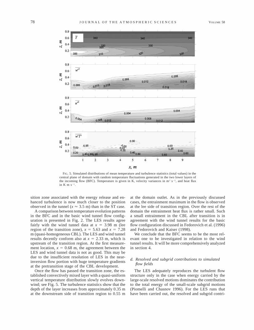
FIG. 5. Simulated distributions of mean temperature and turbulence statistics (total values) in thecentral plane of domain with random temperature fluctuations generated in the two lower layers ofthe incoming flow (BFC). Temperature is given in K, velocity variances in m2 s22, and heat fluxin K m s21.

sition zone associated with the energy release and en-hanced turbulence is now much closer to the positionobserved in the tunnel (x ø 3.5 m) than in the ST case.

A comparison between temperature evolution patternsin the BFC and in the basic wind tunnel flow config-uration is presented in Fig. 2. The LES results agreefairly with the wind tunnel data at x 5 3.98 m (leeregion of the transition zone), x 5 5.63 and x 5 7.28m (quasi-homogeneous CBL). The LES and wind tunnelresults decently conform also at x 5 2.33 m, which isupstream of the transition region. At the first measure-ment location, x 5 0.68 m, the agreement between theLES and wind tunnel data is not as good. This may bedue to the insufficient resolution of LES in the near-inversion flow portion with huge temperature gradientsat the pretransition stage of the CBL development.

Once the flow has passed the transition zone, the es-tablished convectively mixed layer with a quasi-uniformvertical temperature distribution slowly evolves down-wind; see Fig. 5. The turbulence statistics show that thedepth of the layer increases from approximately 0.35 mat the downstream side of transition region to 0.55 m

at the domain outlet. As in the previously discussedcases, the entrainment maximum in the flow is observedat the lee side of transition region. Over the rest of thedomain the entrainment heat flux is rather small. Sucha small entrainment in the CBL after transition is inagreement with the wind tunnel results for the basicflow configuration discussed in Fedorovich et al. (1996)and Fedorovich and Kaiser (1998).

We conclude that the BFC seems to be the most rel-evant one to be investigated in relation to the windtunnel results. It will be more comprehensively analyzedin section 4.

d. Resolved and subgrid contributions to simulatedflow fields

The LES adequately reproduces the turbulent flowstructure only in the case when energy carried by thelarge-scale resolved motions dominates the contributionto the total energy of the small-scale subgrid motions(Piomelli and Chasnov 1996). For the LES runs thathave been carried out, the resolved and subgrid contri-


FIG. 6. Resolved and subgrid contributions to the vertical velocity variance and turbulent ki-nematic heat flux in the central plane of domain (BFC). Velocity variances are given in m2 s22

and heat flux in K m s21.

butions to different turbulence statistics have been eval-uated separately. In Fig. 6, we show distributions ofresolved and subgrid components of the vertical velocityvariance and kinematic heat flux along the domain inthe BFC.

In the main portion of the simulation domain, theresolved-scale contributions to both statistics are defi-nitely larger than the subgrid ones. Within the transitionregion and throughout the quasi-homogeneous CBL thatdevelops downwind, the contributions by resolved flowcomponents are clearly dominant. The major part of thenegative entrainment flux at the downwind side of tran-sition region is maintained by the resolved motions.Before the transition stage, at x , 1 m, the dominanceof the resolved contributions is not as clear. The re-solved-scale motions are not yet developed in this flowregion (this is especially noticeable in the w92 pattern),and a substantial part of turbulence exchange occurs onthe subgrid-scale level.

4. Turbulence structure in the basic flow case

Important information concerning the structure of tur-bulence at different stages of the CBL development can

be obtained from the joint analysis of the numericallysimulated turbulence fields and flow patterns visualizedin the wind tunnel CBL. Visualization of the turbulencestructure in the wind tunnel flow has been realized bymeans of the laser light sheet technique as described inFedorovich et al. (1996) and Fedorovich and Kaiser(1998). A neutrally buoyant fog of tracer particles il-luminated by a laser beam is used to portray the tur-bulence pattern. Assuming that the turbulent motion isadequately represented by the moving fog particles, onemay compare the computed instantaneous flow patternswith the laser sheet visualizations.

First we consider the instantaneous LES patterns oftemperature and vertical velocity corresponding to theBFC. They are presented in Fig. 7. One may notice thatat the stage of the nonmixed unstable layer (x , 3.5 m)the thermal plumes rising from the surface are smalland relatively densely packed. A pool of the cooler airis clearly visible above the hot near-surface layer. Far-ther downstream, the sizes of bulb-shaped plumes in-crease. At the same time, the plumes get detached fromeach other and zones of cooler descending air (down-drafts) grow between them. The downdrafts are well


FIG. 7. Instantaneous temperature and vertical velocity distributions in the central plane of domain (BFC). Temperature is given in K andvelocity in m s21.

displayed in the vertical velocity pattern. The horizontalscales of updrafts and downdrafts in the considered flowregion are approximately the same. The temperature andvelocity fields below the inversion are well correlated:the updrafts transport a warm air from the floor, whilethe compensating downdrafts carry cooler air. The cap-ping inversion remains practically unaffected by thesesmall-scale convective motions.

Within the range 3.5 , x , 5.5 m the flow passesthrough the transition zone. Here, the release of potentialenergy accumulated in the unstable flow below the in-version initiates active upward and downward motionsthat provide the effective mixing of air below the in-version. In addition, these motions perturb the inversionand stimulate the entrainment of the warm air fromabove the inversion down into the convectively mixedlayer. In the bulk of the layer, the main component ofmotion is directed upward, and the updrafts of hot air(in this stage they may be already qualified as convectivethermals) dominate the narrower downdrafts. Closer tothe top of the layer, in the entrainment zone, the down-drafts that transport warmer air downward are becomingwider at the expense of thermals, the horizontal dimen-sions of which decrease with height.

Downwind of the transition zone, the proportion be-tween the dimensions of warm updrafts (thermals) andcool downdrafts is different compared to the pretran-sition flow phase. The flow pattern here consists of vastareas with relatively weak downward motions separatedby the narrow and strong thermals that vertically piercethe whole layer. Such proportions between the areas ofupward and downward motions are in good agreementwith the atmospheric CBL observations presented in

Lenschow and Stephens (1980) and Stull (1988). Thevelocity and temperature fields inside the main portionof the established CBL are still well correlated, but thetemperature pattern at this stage is much less variablethan the pattern in the pretransition region. The inver-sion in the posttransition phase looks quite convolutedand gets progressively weaker due to erosion caused bythe rising thermals.

The next group of plots (Fig. 8) shows instantaneoustemperature patterns derived from the LES in compar-ison with the wind tunnel flow visualizations. The up-permost pair of plots refers to the pretransition flowregion (window 2, x 5 2.33 m). The second pair ofplots (window 3, x 5 3.98 m) shows turbulence patternswithin the transition region. Finally, the third pair (win-dow 4, x 5 5.63 m) refers to the stage of the fullydeveloped convectively mixed layer.

Within the considered fetch range, the scales and ge-ometry of convective elements undergo substantialchanges. At the first location, the buoyant plumes in theunstable near-surface layer are rather small and only afew of them extend up to the capping inversion. In thewind tunnel visualization pattern, the peculiar, bubble-or fingerlike finescale convective elements can be ob-served at the top of the rising plumes. In the temperaturepattern from the LES, the laterally elongated pools ofcool nonmixed air are seen above the patchy blanket ofhot air adjacent to the surface. The capping inversionin the pretransition stage is looking quite strong.

Further development of the turbulence structure inthe tunnel is marked by the merging of plumes into thecolumnlike buoyant thermals, which are bigger andstronger than the plumes. The thermals and associated


FIG. 8. Evolution of thermal structure in the BFC. Instantaneous temperature distributions calculated with the LES (left-hand field of theplot) are presented together with flow visualization patterns from the wind tunnel (right-hand field). Calculations and visualizations refer tothree transverse cross sections located at different distances from the inlet.

cool downdrafts provide strong mixing in the transitionregion and effectively destroy the capping inversion.This is clearly illustrated in the LES pattern referringto the transition region (x 5 3.98 m). Both LES andwind tunnel patterns display deep penetration of ther-mals in the stably stratified fluid above the inversion.The horizontal dimensions of thermals typically de-crease with height, which is consistent with our previousobservations (see Fig. 7) and with lidar images of ther-mals in the atmospheric CBL (Hooper and Eloranta1986). It is remarkable that the tops of newborn thermals

at x 5 3.98 m are composed of the finescale buoyantelements looking like the ones atop the convectiveplumes in the pretransition region, at x 5 2.33 m. Thesesmall-scale elements penetrate through the inversionahead of the main body of the thermal.

The LES patterns do not possess a sufficient reso-lution to reproduce the aforementioned finescale ele-ments. Nevertheless, one can notice that characteristicscales of the structures reproduced by the LES growwith x, whereas the small-scale structure elements dis-appear. Downwind of the transition region, at x 5 5.63


FIG. 9. Variances of the (a) longitudinal and (b) vertical velocity components from the present study (BFC, total values) in comparisonwith data from other CBL studies. The LES results for different locations along the domain are shown by markers: open squares correspondto x 5 3.98 m, triangles to x 5 5.63 m, and rhombuses to x 5 7.28 m. The wind tunnel data for these locations are given by solid lines,dashed lines, and dotted lines, respectively. The LES results of Schmidt and Schumann (1989) for the shear-free CBL are shown by heavysolid lines, atmospheric measurements of Lenschow et al. (1980) and Caughey and Palmer (1979) by filled squares, and data from theDeardorff and Willis (1985) water tank model of the shear-free CBL by asterisks.

m, the thermal contours are becoming less ragged andthe thermals are looking more dome-shaped than theircounterparts in the transition stage. Such redistributionof scales in the temperature patterns obtained by theLES is consistent with the evolution of turbulence-scalestructure in the wind tunnel CBL; see the two lowerplots in Fig. 8.

Let us now proceed to a quantitative comparison ofthe LES results with corresponding wind tunnel dataand with results coming from several other experimentaland numerical studies of the CBL. The data employedfor comparisons are obtained from various sources andfrom different cases of nonsteady, horizontally quasi-homogeneous CBL. It was shown in Fedorovich et al.(1996) and Fedorovich and Kaiser (1998) that the meanflow and turbulence characteristics measured in the post-transition region of the wind tunnel CBL compare fairlywell with data from experimental and model studies ofthe slowly evolving nonsteady CBL.

Before they were plotted, the calculated turbulencecharacteristics had been normalized by the Deardorff(1970) convective scales, which are zi for length, w* 5(bQszi)1/3 for velocity, and T* 5 Qs/w* for temperature.Here, zi is the mixed-layer depth, usually defined aselevation of the heat flux minimum within the entrain-ment zone; b 5 g/T0 is the buoyancy parameter (seesection 2); and Qs is the surface value of the turbulentkinematic heat flux. Despite the well-known shortcom-ings of the mixed-layer scaling (Wyngaard 1992), it hasbeen used for decades as convenient framework forcomparison of measurements from different CBL ex-

periments and for verification of numerical simulationsof the CBL.

The influence of transition on the velocity variancesin the simulated CBL is demonstrated in Fig. 9. At x5 3.98 m (which lies within the transition zone), bothvariances are obviously larger than at the two subse-quent locations downwind of the transition region. Theagreement between the LES and wind tunnel data at x5 5.63 and x 5 7.28 m is very good. Such an agreementis rather unusual for the horizontal velocity variance(Fig. 9a) because this parameter is known to be quitepoorly reproduced by LES of the CBL [see Nieuwstadtet al. (1993), and note the large divergence of data fromother sources in Fig. 9a]. At x 5 3.98 m, the agreementof LES predictions with wind tunnel measurements isnot as good.

With respect to the other data shown in Fig. 9 wenote the following. Compared to the pure shear-freeCBL, which was numerically simulated by Schmidt andSchumann (1989), the larger u92 values at small z arecaused in our case by the additional turbulence pro-duction in the lower CBL portion due to surface shear(Fedorovich et al. 1996). The water tank model andatmospheric measurements both provide rather largevalues of u92 over the whole CBL depth. In the watertank, this is presumably due to the horizontal variationsof heat flux across the bottom of the tank (Schmidt andSchumann 1989). Mesoscale disturbances of the windfield affecting the local turbulence regime in the CBLmay be used as an explanation for the larger atmosphericu92 values (Kaiser and Fedorovich 1998).


FIG. 10. (a) Temperature variance and (b, total values) vertical kinematic heat flux from the present study (BFC) in comparison with datafrom other CBL studies. Notation is the same as in Fig. 9. Atmospheric measurements (filled squares) are represented by data from Caugheyand Palmer (1979).

Within the entrainment region near the CBL top (z/zi

of the order of 1), two main mechanisms can be re-sponsible for the enhancement of horizontal velocityfluctuations. The first one is a sideward transport of airfrom the thermals decelerated by the inversion layer andthe second one is an elevated wind shear (its effect onthe CBL turbulence regime is discussed in Fedorovichet al. 2001). The latter mechanism is likely to be oneof the reasons for the enlarged variances of u in theupper part of the atmospheric CBL. The destruction ofrising thermals by comparatively strong capping inver-sions in the cases of shear-free CBL has been reproducednumerically by Schmidt and Schumann (1989) and inthe water tank by Deardorff and Willis (1985). Suchdestruction results in a clear u92 maximum located atapproximately z/zi 5 1. Our numerical and laboratoryresults for the CBL with a weaker capping inversiongive at most a change (bend) of the slope in the u92

profile at this level.The vertical velocity variance in the CBL is less af-

fected by the nonbuoyant forcing than u92 (Kaiser andFedorovich 1998). This may be a reason for relativelysmall scatter of w92 values from different datasets rep-resented in Fig. 9b. Downstream of the transition zone,our numerical and wind tunnel data show larger valuesof w92 compared to the data from other sources. Thismust be due to the effect of the transition zone. Beforethe numerical simulation has been performed, such en-hancement of velocity variances in the wind tunnel CBLseemed inconsistent with other observations (Fedorov-ich et al. 1996). Thus, the complement of the windtunnel experiments by numerical simulations has beenrather helpful in analyzing the consistency of the ob-servations and understanding the mechanisms that de-termine the CBL turbulence structure.

The effects of transition can be identified also in thesimulated and measured temperature variance and ki-nematic heat flux profiles (Fig. 10). The temperaturevariance inside the entrainment zone is considerablylarger in the transition region (x 5 3.98 m) than through-out the quasi-homogeneous CBL downwind. This is alsothe case of temperature flux caused by entrainment inthe transition zone and at the downwind locations, x 55.63 and x 5 7.28 m. The larger values of both quantitiesin the transition zone are apparently due to the turbu-lence enhancement associated with transition. At x 53.98 m, the relatively big temperature increment acrossthe inversion (see Fig. 2) contributes to the enlargementof temperature fluctuations in addition to the effect oftransition. In the main portion of the CBL, the temper-ature variance and heat flux profiles from the LES andwind tunnel experiments practically coincide for all lo-cations.

The LES and wind tunnel data shown in Fig. 10 seemto diverge near the surface, at z/zi , 0.2. In the case oftemperature variance, this divergence may be caused bypoor reproduction of the near-surface temperature fluc-tuations in the employed LES procedure, which doesnot explicitly account for the subgrid component of T92 .The near-surface drop of the heat flux in the wind tunnelcase can be explained by the insufficient developmentof turbulence near the wind tunnel floor and by certainmeasurement problems discussed in Fedorovich et al.(1996).

The temperature variances presented in Fig. 10a ex-plicitly show the effects of inversion strength and outerflow stability on the magnitude of temperature fluctu-ations at the CBL top. The T92 values from the presentstudy (the case of relatively weak capping inversion)are the smallest at z/zi 5 1, while the water tank and


FIG. 11. Skewness of (a) the resolved-scale vertical velocity and (b) temperature fluctuations from the present study (BFC) in comparisonwith data from other CBL studies. Notation is the same as in Fig. 9. Atmospheric measurements (filled squares) are represented by datafrom Sorbjan (1991).

LES simulations of shear-free CBL with stronger tem-perature gradients across the inversion and above it pro-vide roughly 10 times higher values of T92 at the samedimensionless height.

The atmospheric data on w9T9 in Fig. 10b are stronglyscattered and deviate noticeably from the linear profile.This is probably a result of contributions to the heatbalance of atmospheric CBL by a variety of noncon-vective driving mechanisms (Fedorovich et al. 1996).In the main portion of CBL, at z/zi , 0.9, our laboratoryand numerical data agree well with the w9T9 values fromthe LES and water tank studies of the shear-free CBL.Inside the entrainment zone, however, the magnitude ofthe heat flux in the CBL from the present study is muchsmaller than in the CBL cases with stronger cappinginversions.

Profiles of the skewness of the vertical velocity andtemperature fluctuations are shown in Fig. 11. Theskewness of the vertical velocity fluctuations (Fig. 11a)is positive in the main portion of CBL. This reflects acharacteristic feature of the turbulent convection struc-ture, which is composed of narrow, fast thermals andbroad, slow downdrafts. The vertical velocity skewnessderived from the atmospheric measurements is quiteuniform in the vertical. Such uniformity points to a morehomogeneous structure of up- and downdrafts in theatmosphere compared to the CBL cases reproduced nu-merically and in the laboratory. The comparativelysmall values of the w skewness predicted by LES atsmall z apparently result from insufficient resolution ofemployed LES procedure in the near-surface region ofthe CBL, where the subgrid effects play an importantrole (see also Fig. 5).

The distribution of the w skewness at z/zi . 1 in Fig.11a shows that at the top of atmospheric CBL the up-

ward component of turbulent motion (positive w9) is inan approximate balance with the downward component(negative w9). At the same time, the vertical velocitiesin the upper portion of wind tunnel CBL are persistentlyskewed positively. In this case, the upward componentof w is maintained by compact and active buoyant el-ements, while the downward component w is associatedwith the thermally nearly neutral and slowly descendingair particles, which contribute only slightly to the nettransport of heat across the inversion (see T skewnessin Fig. 11b). As we have already seen in Fig. 10b, theresulting heat flux of entrainment in this case is rathersmall.

Temperature skewness shown in Fig. 11b reaches itsmaximum approximately in the middle of the convec-tively mixed layer, where the simulation results agreefairly well with the atmospheric data. Close to the sur-face, the skewness values predicted by the LES aremarkedly smaller than their wind tunnel counterparts.As in the case of vertical velocity skewness, this maybe an indication of the inadequate performance of LESin the near-surface sublayer. Above the middle portionof CBL, the computed skewness slowly decays withheight toward z/zi 5 1, which is in good agreement withthe atmospheric results.

The temperature skewness data diverge drastically inthe upper part of the CBL. This is one more manifes-tation of difference between regimes of entrainment inthe wind tunnel CBL and in the atmospheric CBL. Inthe former case, the interaction of relatively narrow andcool thermals with a weak capping inversion leads tovery negatively skewed temperature distribution closeto the CBL top. The earlier discussed buoyant fingerlikeelements rising from the tops of thermals in the windtunnel CBL (see visualization patterns in Fig. 8) may


additionally contribute to the enlargement of tempera-ture skewness in the entrainment zone. The thermals inthe atmospheric CBL with presumably stronger cappinginversion are squashed and effectively destroyed by sta-ble density stratification in the inversion layer. This re-sults in the less skewed temperature distribution at thetop of the atmospheric CBL.

5. Summary and conclusions

We have considered the evolution of turbulence struc-ture in a horizontally developing sheared convectiveboundary layer (CBL) capped by a weak temperatureinversion and with a moderate stability in the turbu-lence-free flow above the CBL. A combination of nu-merical technique (LES) and wind tunnel experimentshas been applied to study the development of this bound-ary layer. Such combination has provided an opportunityto investigate a number of CBL flow regimes, whichhad not been reproduced previously either numericallyor in the laboratory. It has turned out to be helpful alsofor understanding some experimentally observed but notsufficiently explained CBL turbulence features.

The development of the studied CBL occurs in threestages. In the initial stage, the turbulent convection isnot yet fully developed. Next a transition occurs that isassociated with turbulence generation caused by the re-lease of potential energy accumulated during the initialstage. After the transition, the boundary layer developsinto a quasi-homogeneous convectively mixed layer.Location of the transition region and the correspondingchange in turbulence regime are strongly dependent onthe magnitude and distribution of disturbances in theflow at the inlet. The CBL evolution in the pretransitionstage is primarily controlled by the temperature fluc-tuations in the incoming flow. The influence of velocityfluctuations at this stage is subordinate to the effect ofthe temperature inhomogeneities. In the case of no inletdisturbances, the turbulent mixing forced by heat trans-fer from the surface develops rather slowly and a sub-stantial accumulation of the potential energy takes placeduring the pretransition stage in the unstable two-layerfluid system capped by inversion. The release of thisenergy is accompanied by a dramatic enhancement ofturbulence in the comparatively narrow bubble-shapedtransition zone. With the temperature fluctuations intro-duced at the inlet, the pretransition phase is much short-er, and the turbulence enhancement in the transition re-gion is less pronounced.

Maximum values of the upward heat flux are ob-served inside the transition zone while the flow regionwith most intensive entrainment heat flux is slightlyshifted downstream of the transition zone. An analogoushorizontal shift is observed in the temperature variancepattern, where the elevated region with strong temper-ature fluctuations in the inversion layer is displaceddownwind with respect to the temperature variancemaximum associated within the transition. In the flow

section downwind of the transition zone, turbulence lev-els are considerably lower than inside the zone, and theturbulence pattern is characterized by a comparativelyweak horizontal variability.

In the numerically simulated flow case with randomtemperature and velocity disturbances prescribed in allnodes of the inlet plane, a peculiar layered structure isformed in the linearly stratified fluid above the inver-sion. The corresponding temperature pattern above theinversion is built up of relatively thick quasi-mixed lay-ers of constant temperature separated by thin interfaciallayers associated with jumplike temperature changes.Zones of the enlarged temperature fluctuations are con-fined to these interfacial layers, whereas the regions withenhanced velocity fluctuations are located within thequasi-mixed layers.

The numerically simulated CBL case with only tem-perature fluctuations generated in the lower portion ofthe inlet plane has been found to be the best match forthe basic CBL flow configuration reproduced in the windtunnel. The second-order turbulence moments derivedfrom the LES for this case show good agreement withthe wind tunnel measurements. The main features oftransition, including the turbulence enhancement withinthe transition zone, are successfully captured by theLES.

The combined numerical and wind tunnel investi-gation has demonstrated that in the CBL beyond thetransition region the turbulence is noticeably skewedthroughout the whole layer. In the entrainment zone, thetemperature is strongly negatively skewed; meanwhilethe vertical velocity skewness keeps positive values upto the very top of the CBL. Smaller-scale secondarybuoyant elements have been identified at the tops oflarger-scale buoyant plumes and thermals penetratingthrough the capping inversion. The magnitudes of ve-locity and temperature skewness in the entrainment re-gion of the simulated CBL are found to be larger thancorresponding magnitudes in the upper portion of at-mospheric CBL. It is suggested that small values of theentrainment heat flux in the simulated CBL are asso-ciated with the above-specified structural properties ofturbulence in the CBL capped by weak inversion.

Acknowledgments. Financial support provided for thestudy by the Deutsche Forschungsgemeinschaft (DFG)within the Project ‘‘Untersuchung and Parametrisierungder Wechselwirkungen von Skalen der Turbulenz kon-vektiver Grenzschichtstromungen unter Verwendung ei-ner einheitlichen Datengrundlage aus Naturmessungen,Windkanalversuchen und numerischen Modellen’’ isgratefully acknowledged.

REFERENCES

Caughey, S. J., and S. G. Palmer, 1979: Some aspects of turbulencestructure through the depth of the convective boundary layer.Quart. J. Roy. Meteor. Soc., 105, 811–827.


Deardorff, J. W., 1970: Convective velocity and temperature scalesfor the unstable planetary boundary layer and for Raleigh con-vection. J. Atmos. Sci., 27, 1211–1213., 1972: Numerical investigation of neutral and unstable planetaryboundary layers. J. Atmos. Sci., 29, 91–115., 1980: Stratocumulus-capped mixed layers derived from a three-dimensional model. Bound.-Layer Meteor., 18, 495–527., and G. E. Willis, 1985: Further results from a laboratory modelof the convective planetary boundary layer. Bound.-Layer Me-teor., 32, 205–236.

Fedorovich, E., and R. Kaiser, 1998: Wind tunnel model study ofturbulence regime in the atmospheric convective boundary layer.Buoyant Convection in Geophysical Flows, E. J. Plate et al.,Eds., Kluwer, 327–370., , M. Rau, and E. Plate, 1996: Wind-tunnel study of tur-bulent flow structure in the convective boundary layer cappedby a temperature inversion. J. Atmos. Sci., 53, 1273–1289., F. T. M. Nieuwstadt, and R. Kaiser, 2001: Numerical and lab-oratory study of horizontally evolving convective boundary lay-er. Part II: Effects of elevated wind shear and surface roughness.J. Atmos. Sci., in press.

Hooper, W. P., and E. W. Eloranta, 1986: Lidar measurements of windin the planetary boundary layer: The method, accuracy and re-sults from joint measurements with radiosonde and kytoon. J.Climate Appl. Meteor., 25, 990–1001.

Kaiser, R., and E. Fedorovich, 1998: Turbulence spectra and dissi-pation rates in a wind tunnel model of the atmospheric convec-tive boundary layer. J. Atmos. Sci., 55, 580–594.

Lenschow, D. H., 1998: Observations of clear and cloud-capped con-vective boundary layers, and techniques for probing them. Buoy-ant Convection in Geophysical Flows, E. J. Plate et al., Eds.,Kluwer, 185–206., and P. L. Stephens, 1980: The role of thermals in the convectiveboundary layer. Bound.-Layer Meteor., 19, 509–532., J. C. Wyngaard, and W. T. Pennel, 1980: Mean-field and second-moment budgets in a baroclinic, convective boundary layer. J.Atmos. Sci., 37, 1313–1326.

Mason, P. J., 1989: Large-eddy simulation of the convective atmo-spheric boundary layer. J. Atmos. Sci., 46, 1492–1516.

Moeng, C.-H., 1984: A large-eddy simulation for the study of plan-etary boundary layer turbulence. J. Atmos. Sci., 41, 2052–2062.

Nieuwstadt, F. T. M., 1990: Direct and large-eddy simulation of freeconvection. Proc. Ninth Int. Heat Transfer Conf., Jerusalem,Israel, American Society of Mechanical Engineering, 37–47., and R. A. Brost, 1986: Decay of convective turbulence. J.Atmos. Sci., 43, 532–546., P. J. Mason, C.-H. Moeng, and U. Schumann, 1993: Large-eddy simulation of the convective boundary layer: A comparisonof four computer codes. Turbulent Shear Flows 8, F. Friedrichet al., Eds., Springer-Verlag, 343–367.

Ohya, Y., and T. Uchida, 1999: Wind tunnel study and DNS of stableboundary layers and convective boundary layers in the atmo-sphere. Turbulence and Shear Flow Phenomena—1, S. Banerjeeand J. K. Eaton, Eds., Begell House, 589–594., K. Hayashi, S. Mitsue, and K. Managi, 1998: Wind tunnelstudy of convective boundary layer capped by a strong inversion.J. Wind Eng., 75, 25–30.

Pearson, H. J., and P. F. Linden, 1983: The final stage of decay ofturbulence in stably stratified fluid. J. Fluid Mech., 134, 195–203.

Piomelli, U., and J. R. Chasnov, 1996: Large-eddy simulations: The-ory and applications. Turbulence and Transition Modelling, M.Hallback et al., Eds., Kluwer, 269–336.

Rau, M., and E. J. Plate, 1995: Wind tunnel modelling of convectiveboundary layers. Wind Climate in Cities, J. E. Ermak et al., Eds.,Kluwer, 431–456.

Schmidt, H., and U. Schumann, 1989: Coherent structure of the con-vective boundary layer derived from large-eddy simulations. J.Fluid. Mech., 200, 511–562.

Sorbjan, Z., 1991: Evaluation of local similarity functions in theconvective boundary layer. J. Appl. Meteor., 30, 1565–1583.

Stull, R. B., 1988: An Introduction to Boundary Layer Meteorology.Kluwer Academic Publishers, 666 pp.

Wyngaard, J. C., 1992: Atmospheric turbulence. Annu. Rev. FluidMech., 24, 205–233., and R. A. Brost, 1984: Top-down and bottom-up diffusion ofa scalar in the convective boundary layer. J. Atmos. Sci., 41,102–112.

ohio higher education funding commission - ohio shared services

Documents