ohio department of transportation - dot.state.oh.us presentations/wednesd… · ohio department of...
TRANSCRIPT
Ohio Department of Transportation
John R. Kasich, Governor Jerry Wray, Director
Development of CPT Spread Footing Direct Design Methodology for ODOT
October 26, 2016
Alexander B.C. Dettloff, P.E.Foundations Engineer
Division of EngineeringOffice of Geotechnical Engineering

2ODOT CPT Rig

3
ODOT CPT Rig
Manufactured by A.P. Van den Berg
Track-Mounted CPT unit Hyson 200 kN
VTS-D4-3550-700-TM30 Crawler
John Deere diesel engine, 93kW = 125 hp
40 1039mm CPT Rods = 41.56m = 136.36’
Maximum Push = 200 kN = 45 kips
15cm2 Type 2 Piezo-Cone w/ Seismic Module
Seismic Hammer Trigger Beam on jacks
ODOT CPT Rig

4ODOT CPT Rig

5CPT Exploration

6CPT Probe

7CPT Probe

8CPT Probe

9CPT Probe

10CPT Probe

11CPT Probe

12CPT Probe
13
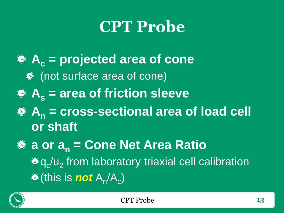
CPT Probe
Ac = projected area of cone
(not surface area of cone)
As = area of friction sleeve
An = cross-sectional area of load cell
or shaft
a or an = Cone Net Area Ratio
qc/u2 from laboratory triaxial cell calibration
(this is not An/Ac)
CPT Probe
14
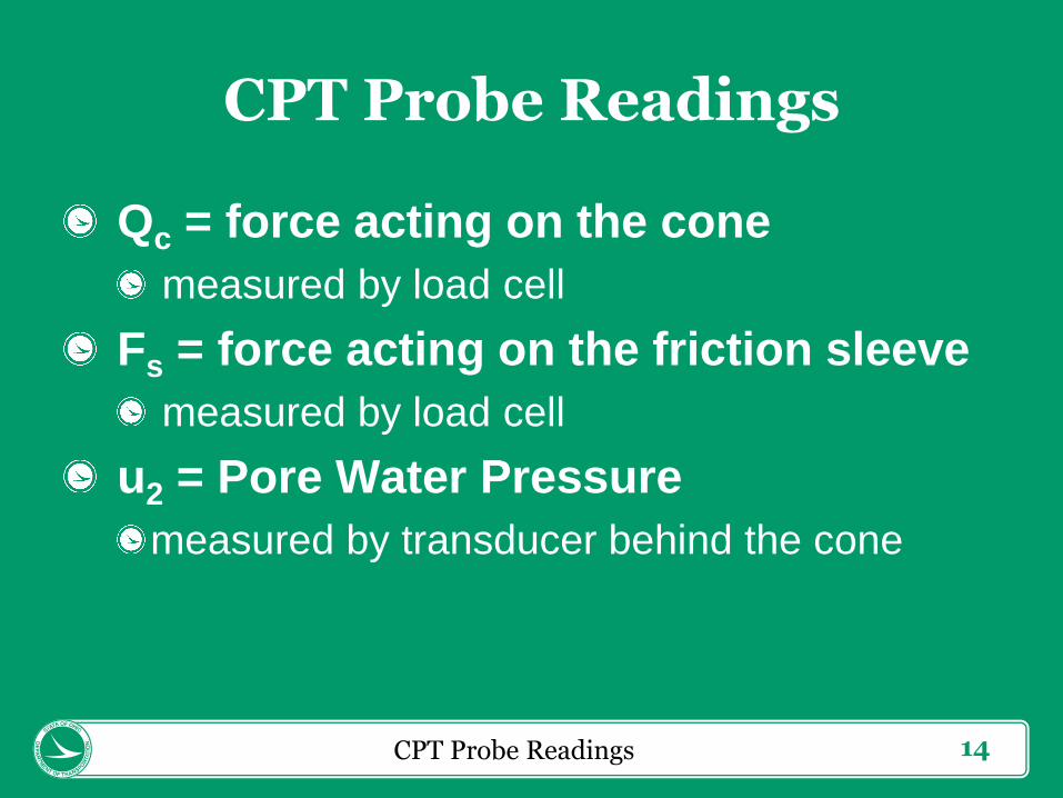
CPT Probe Readings
Qc = force acting on the cone
measured by load cell
Fs = force acting on the friction sleeve
measured by load cell
u2 = Pore Water Pressure
measured by transducer behind the cone
CPT Probe Readings
15
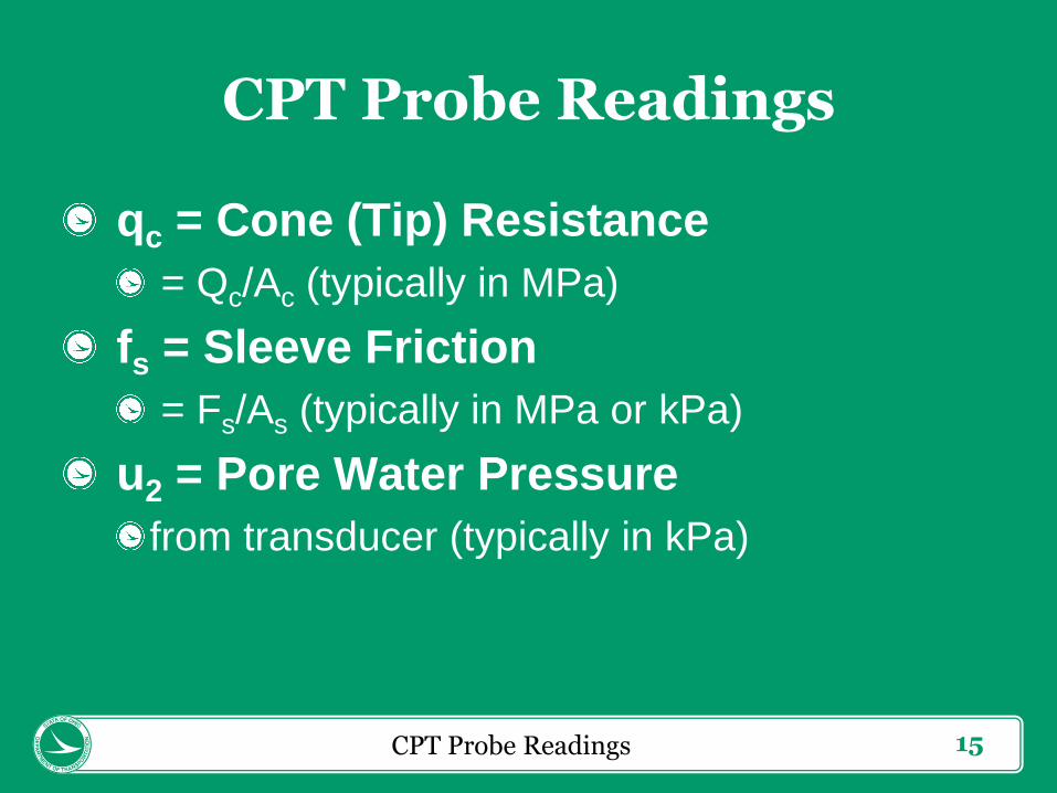
CPT Probe Readings
qc = Cone (Tip) Resistance
= Qc/Ac (typically in MPa)
fs = Sleeve Friction
= Fs/As (typically in MPa or kPa)
u2 = Pore Water Pressure
from transducer (typically in kPa)
CPT Probe Readings

16CPT Probe Readings

17CPT Cone (Tip) Net Area Ratio

18CPT Cone (Tip) Net Area Ratio

19Corrected Tip Resistance
qc is not necessarily directly useful
Need to correct for pore water pressure
qt = Corrected Tip Resistance
= qc + u2(1-a)
20
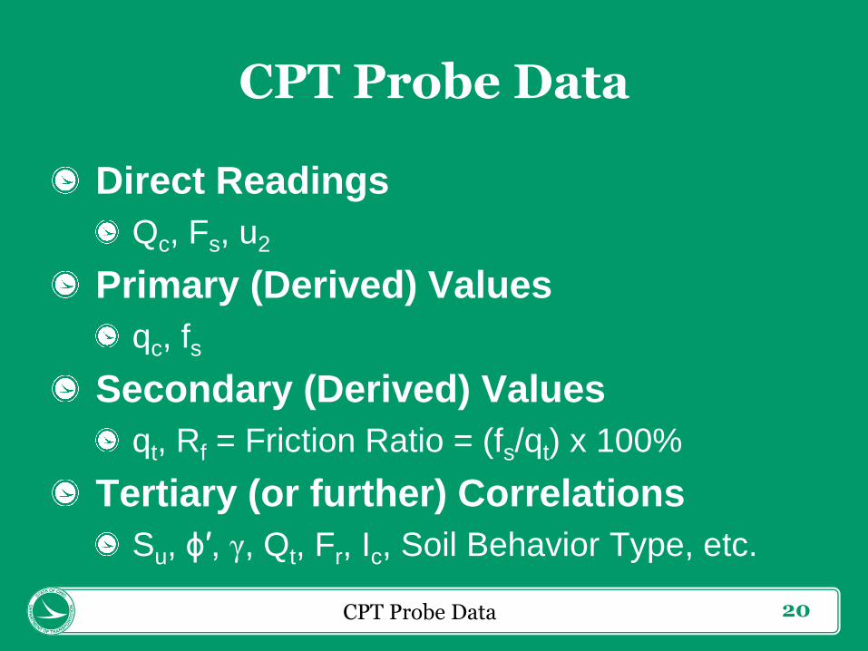
CPT Probe Data
Direct Readings
Qc, Fs, u2
Primary (Derived) Values
qc, fs
Secondary (Derived) Values
qt, Rf = Friction Ratio = (fs/qt) x 100%
Tertiary (or further) Correlations
Su, ϕ′, γ, Qt, Fr, Ic, Soil Behavior Type, etc.
CPT Probe Data

21
CPT Probe Data
Correlations exist for the following:
Su, undrained shear strength
ϕ′, effective internal friction angle
γ, soil unit weight
Soil Behavior Type (SBT)
Qt, Normalized Cone Resistance
Fr, Normalized Friction Ratio
Ic, Soil Behavior Type Index
N60, SPT blow count normalized at ER 60%
CPT Probe Data

22
CPT Probe Data
Correlations exist for the following:
St, soil sensitivity
OCR, overconsolidation ratio
Ko, in-situ stress ratio
Dr, Relative Density
ψ, state parameter
E, Young’s modulus
k, coefficient of permeability
consolidation characteristics (cv, ch, M)
CPT Probe Data

23CPT Direct Design

24CPT Direct Design

25CPT Direct Design
26CPT Direct Design

27CPT Direct Design

28CPT Direct Design

29CPT Direct Design

30CPT Direct Design

31CPT Direct Design

32CPT Direct Design

33CPT Direct Design
Ic (s/B)max
≤1.8 12%
2.0 11%
2.2 10%
2.3 9%
2.4 8%
2.4 7%
2.5 6%
2.5 5%
2.8 4%
≥3.0 3%
(s/B)max versus Ic

34CPT Direct Design

35CPT Direct Design

36CPT Direct Design

37
This is for Ultimate Capacity of the foundation, but we
don’t want an ultimate capacity foundation failure to
occur!
We have two options:
Use a resistance factor to limit the ultimate capacity to a
Strength I Limit State factored resistance.
Limit the deformation based on Service Limit
requirements to get to a Service I Limit State nominal
resistance.
We looked at both by comparing the results of CPT
direct design to the results of the Terzaghi bearing
equation, using correlated soil properties.
CPT Direct Design

38
For the first case (Strength Limit State), we have
qn = qult = qtnet avg. × hs × (s/B)max
For the second case (Service Limit State), we have
qn = qall = qtnet avg. × hs × (s/B)lim,
where (s/B)lim = 0.01 typically,
which equates to (s/B)0.5 = 0.1
or (s/B)lim = (slim/B)
where slim = 1.00 inch (or less, depending on
serviceability requirements of the structure).
For both cases, qtnet avg. = the average qtnet over 1.5B below
the foundation elevation.
CPT Direct Design

39CPT Direct Design

40
CPT Direct Design Inputs
Backfill Soil (bf):
γbf, φbf, δbf, βbf, αbf => ka, EH, EV
Foundation Soil (f):
γf, φf, δf, Suf, c′f, qtnet, Ic => hs, (s/B)max
Surcharge Soil (q):
γq
CPT Direct Design Inputs
41
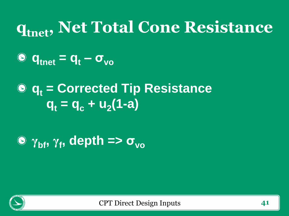
qtnet, Net Total Cone Resistance
qtnet = qt – σvo
qt = Corrected Tip Resistance
qt = qc + u2(1-a)
γbf, γf, depth => σvo
CPT Direct Design Inputs

42
Ic, Soil Behavior Type Index
Ic = ((3.47 - log Qt)2 + (log Fr + 1.22)2)0.5
Qt = normalized cone penetration
resistance (dimensionless)
= (qt – σvo)/σ′vo
Fr = Normalized Friction Ratio (%)
= (fs/(qt – σvo)) x 100%
Ic is used in various other correlations
CPT Direct Design Inputs

43
Ic, Soil Behavior Type Index
Generally,
Ic < 0.5 = Gravel (A-1-a)
Ic = 0.5-1.5 = Sandy Gravel (A-1-b)
Ic = 1.5-2.0 = Sand to Silty Sand (A-3)
Ic = 2.0-2.5 = Sandy Silt to Silt (A-4)
Ic = 2.5-3.0 = Silt and Clay to Silty Clay (A-6)
Ic > 3.0 = Clay (A-7)
Ic = 2.0 is the approximate dividing line
between Granular and Cohesive soils.
CPT Direct Design Inputs
44
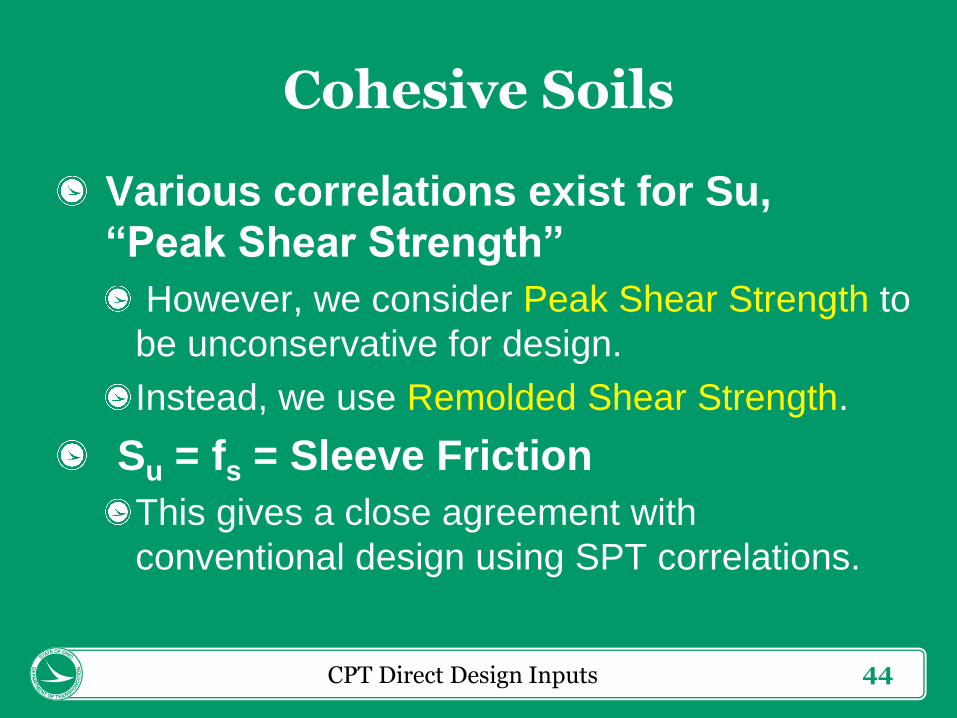
Cohesive Soils
Various correlations exist for Su,
“Peak Shear Strength”
However, we consider Peak Shear Strength to
be unconservative for design.
Instead, we use Remolded Shear Strength.
Su = fs = Sleeve Friction
This gives a close agreement with
conventional design using SPT correlations.
CPT Direct Design Inputs
45
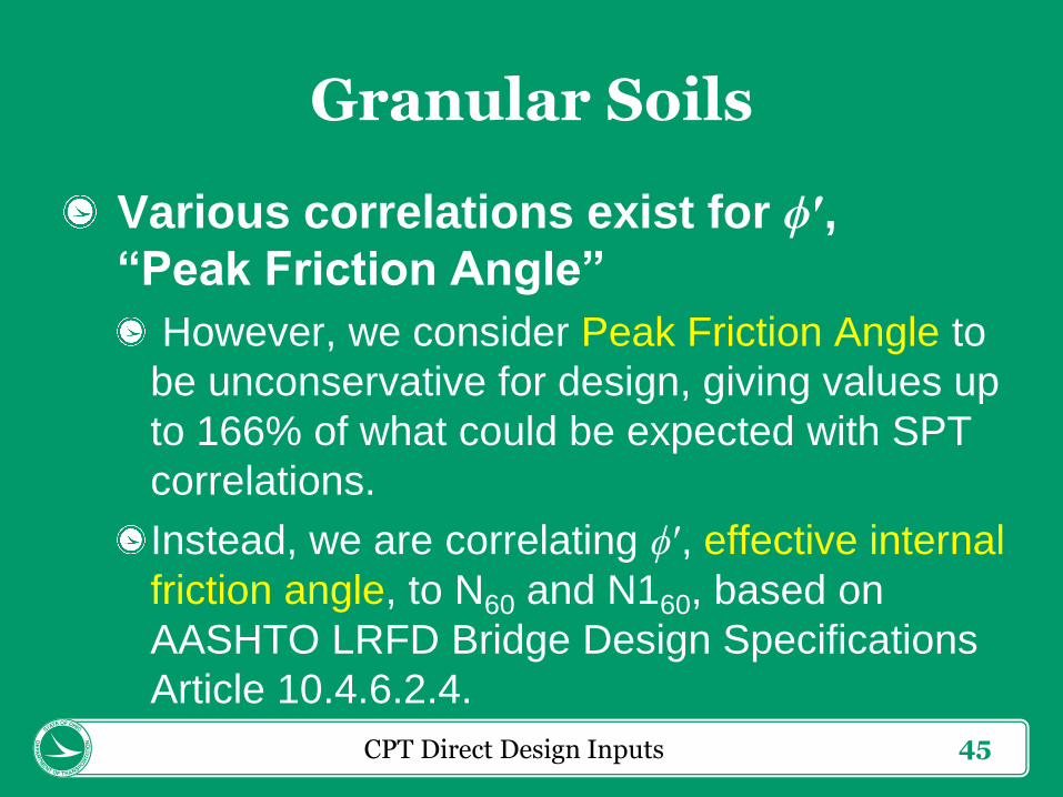
Granular Soils
Various correlations exist for ϕ′,
“Peak Friction Angle”
However, we consider Peak Friction Angle to
be unconservative for design, giving values up
to 166% of what could be expected with SPT
correlations.
Instead, we are correlating ϕ′, effective internal
friction angle, to N60 and N160, based on
AASHTO LRFD Bridge Design Specifications
Article 10.4.6.2.4.
CPT Direct Design Inputs

46
SPT N60 Correlation
We use a correlation developed by
Robertson (2012):
(qt/pa)/N60 = 10(1.1268 – 0.2817Ic)
qt = Corrected Tip Resistance = qc + u2(1-a)
pa = Atmospheric Pressure
Ic = Soil Behavior Type Index
CPT Direct Design Inputs

47
γ, Total Soil Unit Weight
We use a correlation developed by
Robertson (2010):
γ/γw = 0.27 [log Rf] + 0.36 [log(qt/pa)] +1.236
Rf = Friction Ratio = (fs/qt) x 100%
γw = Unit Weight of Water
pa = Atmospheric Pressure
CPT Direct Design Inputs

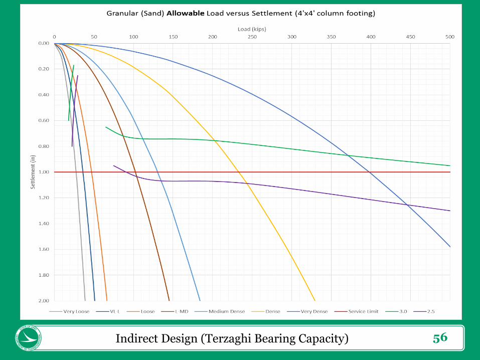
48Indirect Design (Terzaghi Bearing Capacity)

49
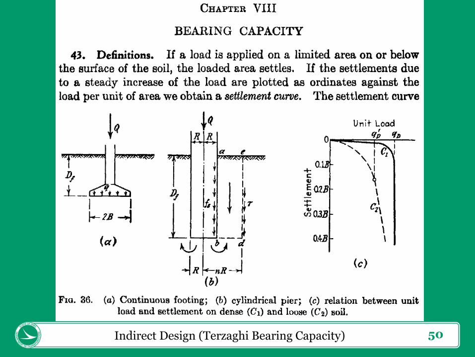
Sand
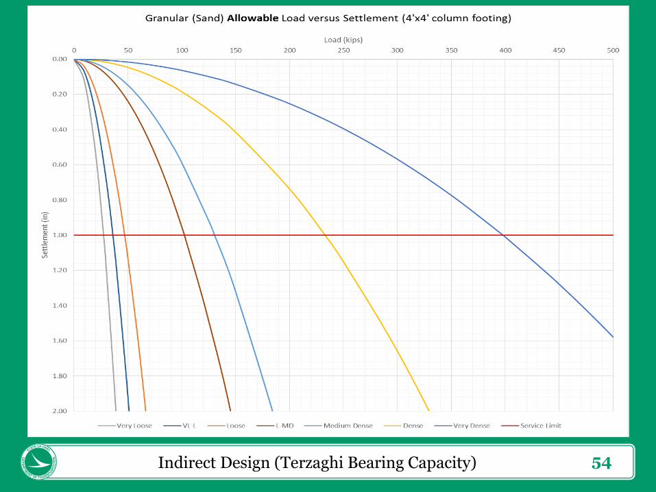
Indirect Design (Terzaghi Bearing Capacity)
50Indirect Design (Terzaghi Bearing Capacity)

51Indirect Design (Terzaghi Bearing Capacity)

52Indirect Design (Terzaghi Bearing Capacity)

53Indirect Design (Terzaghi Bearing Capacity)
54Indirect Design (Terzaghi Bearing Capacity)
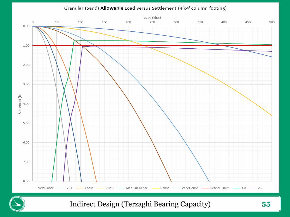
55Indirect Design (Terzaghi Bearing Capacity)
56Indirect Design (Terzaghi Bearing Capacity)

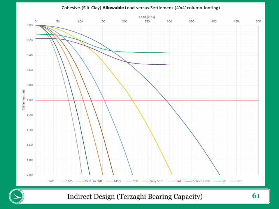
57
Cohesive Soil
Indirect Design (Terzaghi Bearing Capacity)

58Indirect Design (Terzaghi Bearing Capacity)

59Indirect Design (Terzaghi Bearing Capacity)

60Indirect Design (Terzaghi Bearing Capacity)
61Indirect Design (Terzaghi Bearing Capacity)

62
Conclusions
Terzaghi and Mayne essentially agree
for ultimate strength of denser granular
soils (Medium Dense to Very Dense).
Terzaghi bearing with FS = 3.0 or 2.5 straddles
the 1.0-inch displacement line per Mayne.
Deflection (Service) and Strength limit behavior
are in conformance for these soils (neither
really controls over the other).
Mayne versus Terzaghi

63
Conclusions
For looser granular soils (Very Loose to
Loose) Terzaghi General Shear Failure
is extremely unconservative (this is
acknowledged by Terzaghi).
Terzaghi Local Shear Failure is conservative
compared to Mayne (by a factor of around 2).
Deflection does not control in bearing capacity
design of footings by Local Shear Failure.
Mayne versus Terzaghi

64
Conclusions
For low-plasticity cohesive soils (A-4a
or A-6a) Terzaghi bearing capacity is
conservative compared to Mayne.
In the ultimate state, Terzaghi bearing capacity
is conservative by a factor of around 2).
In the service state, Terzaghi bearing capacity
is conservative by a factor of from 2 to 5).
Deflection does not control in footing design in
these soils by Terzaghi bearing capacity.
Mayne versus Terzaghi
65
Conclusions
For looser granular soils and low-
plasticity cohesive soils (A-4a or A-6a)
we could realize a substantial savings
in bearing capacity design by using a
displacement-based CPT Direct Design
methodology.
Mayne versus Terzaghi

66
Direct Design
How to fit a displacement-dependent
design method into an LRFD Limit State
framework?
For Service Limit State, no problem:
Compare Service Limit State Nominal
Load with Allowable Load at (s/B)lim
pn ≤ pall = qn = qall
Trickier at the Strength Limit State
Direct Design Methodology

67Direct Design Methodology

68Direct Design Methodology

69Direct Design Methodology

70Direct Design Methodology

71Direct Design Methodology

72Direct Design Methodology
73Direct Design Methodology

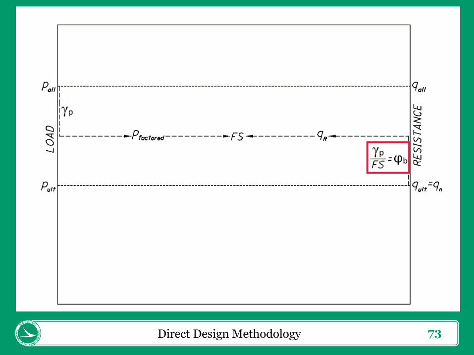
74
Strength Limit State
Service Load = pn
Strength Load = pfactored
pn × γp = pfactored (γp = pfactored / pn)
qult = qtnet avg. × hs × (s/B)max = qn
qall = qtnet avg. × hs × (s/B)lim
FSmin = qult / qall
Direct Design Methodology

75
Strength Limit State
ϕb = γp / FSmin
(ϕb is variable)
qR = ϕb × qn = ϕb × qult
pfactored ≤ qR
FS = qult / pn
FS ≥ FSmin
Direct Design Methodology

76
Example: Medium Dense Sand with Service Limit State load of 100 kips
pn = 100 kips
pfactored = 147 kips
γp = pfactored / pn = 1.47
qult = 313.15 kips = qn
qall = 130.48 kips (at 1.00 inch settlement) = pall
pn ≤ pall OK Service Limit State
FSmin = qult / qall = 2.40
ϕb = γp / FSmin = 0.61
qR = ϕb × qn = 0.61 x 313.15 kips = 191.80 kips
pfactored ≤ qR OK Strength Limit State
Direct Design Methodology

77
References
AASHTO. (2014). “LRFD Bridge Design Specifications.”
7th Edition, AASHTO, Washington, DC.
ASTM D5778-12. (2012). “Standard Test Method for
Electronic Friction Cone and Piezocone Penetration
Testing of Soils.” ASTM International, West
Conshohocken, PA, www.astm.org.
Hansen, J.B. (1970) “A Revised and Extended Formula
for Bearing Capacity”, Bulletin No. 28, Danish
Geotechnical Institute, Copenhagen.
References
78
References
Mayne, P. and Woeller, D. (2014) "Generalized Direct
CPT Method for Evaluating Footing Deformation
Response and Capacity on Sands, Silts, and Clays." Geo-
Congress 2014 Technical Papers: pp. 1983-1997.
Munfakh, G., A. Arman, J. G. Collin, J. C.-J. Hung, and R.
P. Brouillette. (2001) “Shallow Foundations Reference
Manual,” FHWA-NHI-01-023. Federal Highway
Administration, U.S. Department of Transportation,
Washington, DC.
NCHRP (2007) “Synthesis 386: Cone Penetration
Testing.” Transportation Research Board, Washington,
DC, www.TRB.org.
References

79
References
Robertson, P.K., Cabal, K.L. (2014). “Guide to Cone
Penetration Testing for Geotechnical Engineering.” 6th
Edition, Gregg Drilling & Testing, Inc., Signal Hill, CA.
Terzaghi, Karl (1943), Theoretical Soil Mechanics, J.
Wiley & Sons, New York.
Vesic, A.S. (1975), Chapter 3, Bearing Capacity of
Shallow Foundations, Foundation Engineering Handbook,
First Edition, H.F. Winterkorn and H.T. Fang, eds., Van
Nostrand Reinhold Company, New York, NY, pp. 121-147.
References

80
Thank You
Questions?
Comments?
End of Presentation