of transport finance private infrastructure projects - vtt · finance of road infrastructure...

VTT P

UB

LICA

TION

S 624Private finance of transport infrastructure projects

Pekka Leviäkan

gas

ESPOO 2007ESPOO 2007ESPOO 2007ESPOO 2007ESPOO 2007 VTT PUBLICATIONS 624

Pekka Leviäkangas

Private finance of transportinfrastructure projects

Value and risk analysis of a Finnish shadowtoll road project

There is a growing interest to find ways and methods to finance capitalinvestments in infrastructure by deploying private capital. Enteringprivate capital into transport infrastructure planning, construction, andmaintenance markets requires that the investors' behaviour and motivesare understood. Private sector financing of infrastructure and otherlarger-scale investments have increasingly taken the form of projectfinance. The project cash flows are divided by equity investors, debtinvestors, contractors and suppliers and the users that receive the service.

This research investigates the characteristics of a feasible frameworkfor private finance of road infrastructure projects using one case projectas an example, which is analysed in depth. The research makes an effortto find out whether private finance of road infrastructure projects is ableto bring additional benefits for the state and the project investors and inwhat terms private finance is applicable.

ISBN 978-951-38-6880-2 (soft back ed.) ISBN 978-951-38-6881-9 (URL: http://www.vtt.fi/publications/index.jsp)ISSN 1235-0621 (soft back ed.) ISSN 1455-0849 (URL: http://www.vtt.fi/publications/index.jsp)

Julkaisu on saatavana Publikationen distribueras av This publication is available from

VTT VTT VTTPL 1000 PB 1000 P.O. Box 1000

02044 VTT 02044 VTT FI-02044 VTT, FinlandPuh. 020 722 4404 Tel. 020 722 4404 Phone internat. + 358 20 722 4404Faksi 020 722 4374 Fax 020 722 4374 Fax + 358 20 722 4374

structure

structure

risk

risk

model

model

VTT PUBLICATIONS 624

Private finance of transport infrastructure projects

Value and risk analysis of a Finnish shadow toll road project

Pekka Leviäkangas

Academic dissertation to be presented, with the assent of the Faculty of Technology of the University of Oulu, Department of Industrial Engineering

and Management, for public defence in Lecture Room of VTT, Kaitoväylä 1, Oulu, on March 2nd, 2007, at 12 noon.

ISBN 978-951-38-6880-2 (soft back ed.) ISSN 1235-0621 (soft back ed.)

ISBN 978-951-38-6881-9 (URL: http://www.vtt.fi/publications/index.jsp) ISSN 1455-0849 (URL: http://www.vtt.fi/publications/index.jsp)

Copyright © VTT Technical Research Centre of Finland 2007

JULKAISIJA � UTGIVARE � PUBLISHER

VTT, Vuorimiehentie 3, PL 1000, 02044 VTT puh. vaihde 020 722 111, faksi 020 722 4374

VTT, Bergsmansvägen 3, PB 1000, 02044 VTT tel. växel 020 722 111, fax 020 722 4374

VTT Technical Research Centre of Finland, Vuorimiehentie 3, P.O.Box 1000, FI-02044 VTT, Finland phone internat. +358 20 722 111, fax + 358 20 722 4374

VTT, Kaitoväylä 1, PL 1100, 90571 OULU puh. vaihde 020 722 111, faksi 020 722 2090

VTT, Kaitoväylä 1, PB 1100, 90571 ULEÅBORG tel. växel 020 722 111, fax 020 722 2090

VTT Technical Research Centre of Finland, Kaitoväylä 1, P.O. Box 1100, FI-90571 OULU, Finland phone internat. +358 20 722 111, fax +358 20 722 2090

Technical editing Anni Kääriäinen Edita Prima Oy, Helsinki 2007

http://www.vtt.fi/publications/index.jsp


3

Dedicated to my beloved wife Kirsi, who endured and has been with me all the way � and who got the numbering of

tables and figures in order!

5

Leviäkangas, Pekka. Private finance of transport infrastructure projects. Value and risk analysis ofa Finnish shadow toll road project [Liikenneinfrastruktuurihankkeen yksityisrahoitus. Arvo- ja riskianalyysi sijoitusnäkökulmasta]. Espoo 2007. VTT Publications 624. 238 p. + app. 22 p.

Keywords private finance, transport infrastructure projects, private capital, project risks,project model, cash flow model, risk structure model, Capital Asset PricingModel (CAPM)

Abstract There is a growing interest to find ways and methods to finance capital investments in infrastructure by deploying private capital. Entering private capital into transport infrastructure planning, construction, and maintenance markets requires that the investors� behaviour and motives are understood. Private sector financing of infrastructure and other larger-scale investments have increasingly taken the form of project finance. The project cash flows are divided by equity investors, debt investors, contractors and suppliers and the users that receive the service.

This research investigates the characteristics of a feasible framework for private finance of road infrastructure projects using one case project as an aid, which is analysed in depth. The research makes an effort to find out whether private finance of road infrastructure projects is able to bring additional benefits for the state and the project investors and whether private finance is applicable from the viewpoint of the aforementioned.

The concept of risk is presented in the framework of financial theory. The relevant project cash flows are identified, as their volatility builds the risks of the project. The project cash flows are studied in detail as to how they form the value of the project. One essential outcome is the project model. The empirical model is built in view of the decision making point on case project in 1996, when the bidding for the project was officially initiated. Recent observed, real data is used to validate the project model. The sub-models of the project model include the cash flow model and the risk structure model, the former based on financial theory and Capital Asset Pricing Model, the latter based on the cash

6

flow model and literature on risk. Simulation is used as the primary method of analysis.

The primary source of time series data for economic variables, traffic volumes and road operating and construction is the Finnish Road Administration�s production statistics.

The case project finance is evaluated from multiple angles � what type of projects and what type of investors seem to be appropriate for shadow toll finance. Also some policy recommendations are provided. The private investors can gain by financing infrastructure projects, but it comes with a price, which is always paid by the taxpayers or users. To justify private finance, the beneficial aspects of private capital deployment must be substantial. The projects must be the best projects from a socio-economic viewpoint and not the ones that do not survive the competition in the normal budgetary process.

Different risk factors are behind the long-term value risk and short-term insolvency risk of the project company. Project-specific risk factors are at least as important as economy level factors.

7

Leviäkangas, Pekka. Private finance of transport infrastructure projects. Value and risk analysis ofa Finnish shadow toll road project [Liikenneinfrastruktuurihankkeen yksityisrahoitus. Arvo- ja riskianalyysi sijoitusnäkökulmasta]. Espoo 2007. VTT Publications 624. 238 s. + liitt. 22 s.

Avainsanat private finance, transport infrastructure projects, private capital, project risks,project model, cash flow model, risk structure model, Capital Asset Pricing Model (CAPM)

Tiivistelmä Infrastruktuurin yksityisrahoitus on yleistynyt maailmassa. Yksityisen pääoman käytön edellytykset ja reunaehdot on tunnettava eri rahoitusmahdollisuuksia arvioitaessa. Tällöin myös sijoittajien motiiveja ja käyttäytymissääntöjä on ymmärrettävä syvällisemmin. Projektirahoitus sisältää myös markkinaehtoisen pääomarahoituksen eri muodot. Projektirahoituksessa muodostetaan usein erillinen projektiyhtiö, jonka kassavirrat jakautuvat sijoittajien, alihankkijoiden ja hyödykkeen käyttäjien kesken. Laajoissa infrastruktuurihankkeissa valtio edustaa usein kaikkia käyttäjiä.

Tässä väitöstutkimuksessa muodostetaan käsitys niistä edellytyksistä ja reunaehdoista, jotka mahdollistavat projektirahoituksen. Tutkimuksessa selvite-tään, voidaanko yksityisrahoituksella saavuttaa hyötyjä perinteiseen budjetti-rahoitukseen nähden ja millaisia riskejä yksityisrahoitus sisältää erityisesti sijoittajien näkökulmasta. Riskien analysointi perustuu rahoitus- ja riski-teorioiden viitekehyksiin, ja projektiyhtiön kassavirtojen vaihtelun aiheuttavat tekijät ovat tunnistettuja riskitekijöitä. Projektiyhtiön arvo muodostuu yhtiön kassavirroista, ja niin ollen riskit ovat myös sijoittajien kannalta sijoitusten arvonmuodostuksen riskejä.

Eräänä tutkimustuloksena esitetään projektimalli, joka kuvaa projektiyhtiön arvonmuodostuksen ympäröivien taloudellisten ja teknisten tekijöiden funktiona. Empiirinen malli perustuu vuotta 1996 edeltävään tilastoaineistoon, jolloin valtatie 4 Järvenpää�Lahti -hankkeen suunnittelu, rakentaminen, ylläpito ja rahoitus avattiin kilpailulle. Projektimallin toimivuutta arvioidaan tuoreemmalla empiirisellä aineistolla. Kehitetty malli toimii kohtalaisen hyvin. Projektimalli koostuu useammasta osamallista, kuten kassavirtamallista ja riskimallista.

8

Edellinen perustuu rahoitusteoreettiseen CAP-malliin (Capital Asset Pricing Model) ja jälkimmäinen yleiseen riskiteoriaan.

Tutkimusmenetelminä käytetään tilastollisia regressiomalleja, systeemianalyysia ja mallien simulointia. Tilastoaineistona käytetään pääosin talouden indikaatto-reita kuvaavia julkisia tilastoja ja tiehallinnon tilastoja.

Järvenpää�Lahti-hankkeen rahoitusjärjestelyä arvioidaan eri näkökulmista: millaiset hankkeet ja sijoittajat sopivat vastaaviin hankkeisiin. Hankerahoitusta koskevan päätöksenteon tueksi esitetään joitakin suosituksia. Hankkeet, joiden yhteiskuntataloudellinen hyöty-kustannussuhde on huono, eivät sovellu rahoitettavaksi yksityisellä pääomalla. Yksityisten sijoittajien riskien hinnoittelu voi olla valtiolle, eli veronmaksajille, kallista. Sijoittajien sijoituskohteena infra-struktuurihankkeet voivat olla pitkällä tähtäimellä kohtuullisen riskittömiä, mutta vaadittavat käyttöpääomat ovat niin suuria, että projektiyhtiön maksu-valmiusriskit ovat merkittävät.

9

Acknowledgements

I would like to express my gratitude to all those who have contributed towards this research in the form of data, valuable advice and comments. These persons are the following: road engineer Mr Rauno Kuusela from the Tampere r&d unit of Finnish National Road Administration (Finnra) whose profound expertise was very valuable and whose estimates and evaluations were in many places the starting point for further analyses; chief statistician Mr Pekka Räty from the r&d unit of Finnra, whose advise and discussions are highly appreciated; on many occasions Pekka�s hints saved a lot of work and improved the quality of analysis; road engineer Mr Jyrki Karhula, a colleague from the south-eastern region of Finnra together with Mr Olli Penttinen from Finnra Headquarters who provided valuable comments on maintenance costs; Ms Tarja Tuovinen from the south-eastern region of Finnra was also most helpful and submitted many useful reports and data sources; road engineers Ms Maarit Solla and Ms Marja Rautavirta from Finnra headquarters for providing a lot of useful information; Ms Sirpa Haapamäki, from the Finnra library who has continuously been of service, along with her staff � especially I would like to name Ms Riitta Mäkelä who took care of many practical matters; road master Mr Lasse Kultanen from the Kotka maintenance unit and Mr Tapio Ranta from Finnra Headquarters for providing information on maintenance costs; Ms Anja Koikkalainen and Ms Aila Alahuhtala from the south-eastern region of Finnra and Mr Matti Hämäläinen from Uusimaa region and Ms Ulla Sippola from Häme region for assistance with road, cost and accident data; Mr Veijo Kokkarinen from the Finnra r&d unit who assisted with traffic forecasting data; general manager Mr Tapani Särkkä and Mr Kimmo Tikka from Matrex Ltd. for helping to interpret traffic forecasts and provided support in terms of computer-aided tools; Ms Leena-Marja Ahola from the south-eastern region of Finnra who has partly produced the graphics of this thesis.

The financial support was granted by the Ministry of Transport and Communications and the Järvenpää�Lahti project. Ms Marja Heikkinen-Jarnola, the deputy head of department of the ministry, and Mr Risto Pelttari, project manager for Järvenpää�Lahti, were the key persons to promote this study. I also received help from Ms Nina Raitanen and Ms Johanna Haavisto from the Ministry. All their help and support is appreciated.

10

I also wish to thank my superiors in Finnra, road directors Ville Mäkelä and Antti Rinta-Porkkunen and director Yrjö Pilli-Sihvola, for the flexibility in arranging my duties during the research (not to mention more than 10-year borrowing of a laptop!).

Lappeenranta University of Technology and Neste Foundation are acknowledged with gratitude for financial support. Later my employer VTT Technical Research Centre of Finland and my superiors there, especially technology manager Heikki Kanner, provided me an opportunity to complete this research.

Ms Raija Sahlsted from VTT is acknowledged for helping to get the references in order. Ms Anni Kääriäinen and Ms Tarja Haapalainen from VTT Information Services edited this manuscript to its final format. Ms Arja Wuolijoki designed the cover. Mr Adrian Spencer proofread the language of the manuscript.

I have the pleasure of expressing my gratitude to my early tutor, professor Pentti Talonen at Lappeenranta Institute of Technology, without whose help I would have never gone this far. Not only did he help from a technical point of view, but his supportive advice and recommendations were invaluable. Ms Pirkko Kangasmäki, also from the Institute, is acknowledged for helping with many practical matters concerning the carrying out of the study.

Professor Juha-Pekka Kallunki at University of Oulu is acknowledged for his constructive comments. His expertise and knowledge was of utmost significance in the latter stages of the research process. Professor Harri Haapasalo, my tutor, is acknowledged with deep gratefulness for support and advice that evidently helped to complete this work. His role in summing up the research process and results was crucial.

Professors Antti Talvitie and Marcus Wigan are deeply thanked for their invaluable pre-examination of this thesis. They took the effort and time despite their private and professional obligations.

Thank you all very, very much.

Pekka Leviäkangas

11

Contents

Abstract ................................................................................................................. 5

Tiivistelmä ............................................................................................................ 7

Acknowledgements............................................................................................... 9

List of Figures ..................................................................................................... 15

List of Tables ...................................................................................................... 18

Glossary of terms, abbreviations and symbols.................................................... 21

PART I: INTRODUCTION AND RESEARCH SCOPE................................... 23

1. Introduction................................................................................................... 25 1.1 World of private finance...................................................................... 25 1.2 Policy issues ........................................................................................ 29

1.2.1 Asset privatisation................................................................... 29 1.2.2 Service pricing and user charging ........................................... 31

1.3 Participating private sector in the financing of transport infrastructure .......34 1.4 BOT concept and project finance ........................................................ 37 1.5 Project as real asset investment and capital budgeting problem.......... 44

2. The purpose and scope of this research ........................................................ 47 2.1 Conclusions drawn from privatisation and private finance of

infrastructure........................................................................................ 47 2.2 The research questions and structure of the research .......................... 49 2.3 Expected outcomes and contributions, summary of the research

process ................................................................................................. 51

3. Data and methods ......................................................................................... 55 3.1 Data sources......................................................................................... 55 3.2 Methods ............................................................................................... 56

12

PART II: PROJECT VALUATION AND PROJECT RISK.............................. 59

4. Project valuation ........................................................................................... 61 4.1 Project valuation using CAPM............................................................ 61 4.2 Project cash flow model and stakeholder values ................................. 63 4.3 Cost of capital...................................................................................... 68

5. Risk structure model ..................................................................................... 71 5.1 Different perspectives to risk and classifications of risk models......... 71 5.2 Synthesis � risk structure of a project.................................................. 75

PART III: PROJECT MODEL SPECIFICATION BASED ON EMPIRICAL DATA ................................................................................................................. 79

6. Empirical volatility of economy-wide and project-specific variables .......... 81 6.1 Interest rates......................................................................................... 81 6.2 Traffic demand .................................................................................... 82 6.3 Construction cost risk .......................................................................... 83 6.4 Operating costs .................................................................................... 89

6.4.1 Contract terms and cost structure ............................................ 89 6.4.2 Winter maintenance costs ....................................................... 92 6.4.3 Asphalt pavement maintenance............................................... 95 6.4.4 Other maintenance operations................................................. 97

6.5 Specific risk issues .............................................................................. 99 6.5.1 Disturbances in revenues......................................................... 99 6.5.2 Technical and other risks ...................................................... 100

6.6 Discussion and summary................................................................... 101

7. Interdependence of variables � project framework model.......................... 105 7.1 Introduction ....................................................................................... 105 7.2 Economy-wide relationships ............................................................. 105 7.3 Project-specific relationships............................................................. 112 7.4 Multi-equation project framework model.......................................... 115

8. Full project model components................................................................... 118 8.1 Model assumptions............................................................................ 118 8.2 Economic growth time series model ................................................. 119

8.2.1 Official and documented forecasts........................................ 119 8.2.2 Time series model specification............................................ 120

13

8.3 Forecasting scenarios and simulation process ................................... 124 8.4 Full project model specification (for nominal cash flows) ................ 127

9. Ex ante project beta..................................................................................... 129 9.1 Introduction ....................................................................................... 129 9.2 Review based on un-relaxed empirical data ...................................... 130 9.3 Relaxations and project beta.............................................................. 131

PART IV: SIMULATIONS AND ANALYSES OF SIMULATED DATA .... 133

10. Simulating the case project ......................................................................... 135 10.1 Required capital input........................................................................ 135 10.2 Probability of insolvency and debt capacity...................................... 137 10.3 Determinants of insolvency............................................................... 144 10.4 Project�s cost of capital ..................................................................... 151

10.4.1 Introduction � finding the correct discounting rates for valuations .............................................................................. 151

10.4.2 CAPM-based cost of capital using un-relaxed empirical data ...151 10.4.3 Cost of capital, relaxed estimates.......................................... 156

10.4.3.1 Reference interest rates, relaxed estimates ............... 156 10.4.3.2 Cost of equity............................................................ 157 10.4.3.3 Cost of debt............................................................... 157

10.4.4 Discussion ............................................................................. 161 10.5 Optimal capital structure ................................................................... 164 10.6 Value of the case single-project company......................................... 165 10.7 Determinants of market value............................................................ 171 10.8 The state�s economic positions.......................................................... 175

PART V: SUMMARY OF RESULTS AND EVALUATION......................... 181

11. Risk profile of the case project ................................................................... 183 11.1 Investor risks ..................................................................................... 183 11.2 Risk mitigation strategies and tactics for project investors ............... 188 11.3 State�s risks........................................................................................ 190

12. Evaluation of shadow toll arrangements..................................................... 192 12.1 What kind of projects?....................................................................... 192 12.2 What type of investors? ..................................................................... 194 12.3 About contract arrangements............................................................. 195

14

12.4 Policy recommendations ................................................................... 197

13. Discussion on methodological issues ......................................................... 200 13.1 About the use of CAPM .................................................................... 200 13.2 Project valuation................................................................................ 201 13.3 On project model and its validity ...................................................... 202

14. Recent empirical data.................................................................................. 204 14.1 Project company data ........................................................................ 204 14.2 Model diagnostics � comparison between actual data and

simulation results............................................................................... 205

15. Validation of the research and implications for further research................ 210 15.1 Summary of answers to the research questions ................................. 210 15.2 Validation of the research approach and some generalized findings ......219 15.3 Further research needs ....................................................................... 224

References......................................................................................................... 226

Appendices

Appendix A: Expected operating (maintenance) costs Appendix B: Project description Appendix C: Modeled and observed variables Appendix D: Ex ante project beta � analysis based on un-relaxed empirical data

15

List of Figures

Figure 1. Infrastructure sections and aspects of research content (The 2nd Workshop on Applied Infrastructure Research). ...................................28

Figure 2. Time horizon in different types of contracts........................................38

Figure 3. Cash flows and contractual relations of a privately financed infrastructure project (Dias & Ioannou 1995, p. 405)..........................................40

Figure 4. Current main research fields................................................................48

Figure 5. Summary of the research process � methodological, research process and contribution layers. ...........................................................54

Figure 6. A simplified model of project cash flows. ...........................................64

Figure 7. Classification scheme for descriptive risk models (Shoemaker, 1980). .............................................................................................72

Figure 8. Risk structure of a privately financed civil engineering project (modified from Leviäkangas 1998). .......................................................78

Figure 9. National, regional (Uusimaa region) and road-specific changes of VKT estimates for 1980�1994..........................................................83

Figure 10. Civil engineering works cost index (Hemmilä & Kankainen 1993 and direct information service from Statistics Finland 2006). ...................87

Figure 11. Distribution of project cost estimate changes, large projects (>100 MFIM), n = 18..........................................................................................88

Figure 12. Winter maintenance unit costs in Uusimaa region for 1981�1995; 1995 prices (Finnish Road Administration 1996). ..........................93

Figure 13. Asphalt pavement maintenance costs in Uusimaa region; 1995 prices.......96

Figure 14. Other maintenance costs in Uusimaa region; 1995 prices.................98

Figure 15. GDP cycle of income and expenditure (Lipsey & Chrystal 1995, p. 500)........................................................................106

Figure 16. GDP and national VKT for personal cars excluding heavy vehicles, 1974�1995. ..............................................................................108

Figure 17. Time series of VKT and cost index. ................................................ 110

16

Figure 18. Relative changes of inflation and VKT and their correlation; data for 1966�1995........................................................................ 112

Figure 19. Project-specific demand risk; estimates of national VKT changes and case road�s VKT changes. ................................................... 114

Figure 20. Conceptual project model � an illustration of inter-dependencies of chosen macro and project variables. .............................. 117

Figure 21. GDP forecasting model using autoregressive Box-Jenkins methodology; modelled figures are calculated as one-year-ahead forecasts on the basis of actual figures of the two previous years. ...................122

Figure 22. The autocorrelogram of the time series model. ...............................123

Figure 23. Three simulated GDP forecasts with actual observations, modelled (i.e. predicted) values and simulated scenarios. ................................124

Figure 24. Capital reserves of the project company with different capital structures at the beginning of each year of the concession; V = K = capital reserve (in cash terms). ...........................................................136

Figure 25. Capital reserves of the project company when there is no debt and 605 MFIM equity input; results of 19 simulation runs..................140

Figure 26. The required capital input (y-axis, VAR2) when investors seek 90% succession rate (i.e. less than 10% probability of insolvency) as a function of capital structure (x-axis, VAR1). .....................143

Figure 27. Cost of capital of the project company. ...........................................154

Figure 28. NPV_PI in the case of different unit tolls........................................166

Figure 29. Value of project (Vp). ......................................................................167

Figure 30. The market values of project, debt and equity; unit toll = 0.7 FIM...........168



Figure 33. Returns on project, equity and debt, unit toll = 0.7 FIM. ................169



17

Figure 36. State�s total benefits and costs in shadow toll arrangement when project�s benefit cost ratio varies........................................178

Figure 37. The sensitiveness of state�s economic position to project company capital structure. ....................................................................179

Figure 38. Estimated and observed nominal cash flows of the project company. ...............................................................................................206

Figure 39. Project model and its sub-model components � RQ2.1...................214

Figure 40. Risk determinants, their relationships (dashed arrow lines) and the term structure � RQ2.2, RQ2.3 and RQ3.1. .........................................215

Figure 41. Project returns to the state and investors � RQ3.2; Bs/Cs is the state�s return in shadow toll arrangement and B/C is the socio-economic benefit-cost ratio........................................................................218

18

List of Tables

Table 1. Ways to fund and manage infrastructure (or other) projects (Brealey et al. 1996, p. 27)..................................................................................28

Table 2. Total factor productivity in the UK public sector for 1979�1990; rate of change per annum (%) (Kay 1993)..........................................................30

Table 3. Costs and benefits to public and private sectors (TRB 1988). ..............35

Table 4. Ranking of critical success factors in winning overseas contracts........43

Table 5. Statements and presumptions to be examined; RQ1.1�RQ1.5. ............49

Table 6. Summary of the research scope, questions and methods. .....................53

Table 7. Project cash flows to different stakeholders..........................................65

Table 8. A typology of risks (Griffith-Jones 1993, p. 22). ..................................73

Table 9. Risks and their importance; US contractors� view in 1993 (Kangari 1995). ....................................................................................................74

Table 10. Time series of interest rates (Bank of Finland 1986�1996; Nordiska Ministerådet 1996). .............................................................................82

Table 11. Unit costs of up-dating a semi-motorway to a motorway; million FIM / km, 1995 prices; VAT excluded....................................................84

Table 12. Construction cost time series. .............................................................87

Table 13. Day-to-day winter maintenance costs 1981�1995; overheads excluded (Finnish Road Administration 1996a, pp. 67, 77, 87). .......94

Table 14. Asphalt pavement maintenance costs (inflation adjusted) in three regions for 1981�1995. ..........................................................................96

Table 15. Other maintenance costs in southern road regions for 1981�1995 in 1995 prices......................................................................................................99

Table 16. Regression statistics for Eq.7-1.........................................................107

Table 17. Descriptive statistics for Eq.7-3. ....................................................... 110

Table 18. Regression statistics for Eq.7-4......................................................... 111

Table 19. Regression statistics for Eq.7-5......................................................... 114

19

Table 20. Correlation matrix for macro and project framework model variables. ................................................................................................ 117

Table 21. Regression statistics for Eq.8-1.........................................................121

Table 22. Estimated levered betas of the case project; Tc = 28%.....................131

Table 23. Minimum required capital input; K is total capital, E is equity, D is debt. .........................................................................................136

Table 24. Simulation results with different capital structures and different amounts of capital infusion..........................................................141

Table 25. Statistical parameters of the required capital input model Eq.9-5.....144

Table 26. Determinants of insolvency � results of 26 simulated insolvency cases................................................................................................147

Table 27. Multiple regression results for Eq.9-7...............................................148

Table 28. Stepwise regression summary for Eq.9-7..........................................149

Table 29. Stepwise regression summary � variables� contribution to regression. .....................................................................................................149

Table 30. Variables� correlation matrix (Eq.9-7)...............................................150

Table 31. Computed values for cost of capital. .................................................153

Table 32. Relaxed estimates for cost of equity..................................................157

Table 33. Synthetic rating and spreads for smaller and riskier firms................158

Table 34. Interest coverage; cash flow before interest and taxes divided by interest.............................................................................................159

Table 35. Synthetic estimates of premiums on cost of debt. .............................160

Table 36. After-tax cost of capital estimates; debt capacity assumption relaxed............................................................................................161

Table 37. Summarising the results of cost of capital estimations (after-tax cost of debt).......................................................................................162

Table 38. Estimates of cost of capital for the case project. ...............................163

Table 39. WACC for different unit tolls and capital structures. ........................165

Table 40. Simulations of NPV_PI.....................................................................173

20

Table 41. Summary of stepwise regression for Eq.9-9 � variables� contribution. .....................................................................................173

Table 42. Multiple regression results summary for Eq.9-9...............................174

Table 43. Variables� correlation matrix (Eq.9-9)...............................................174

Table 44. The state�s economic positions in conventional investment and in shadow toll cases. ................................................................175

Table 45. The medium term risks of insolvency and long term risks of low project value..........................................................................187

Table 46. Typical risks for transport infrastructure projects and �risk impact� on the case project................................................................187

Table 47. Estimated and observed nominal cash flows of Nelostie Ltd.; million FIM................................................................................205

Table 48. Observed capital finance. ..................................................................207

Table 49. Statements and presumptions examined; RQ1.1�RQ1.5. .................212

Table 50. The merits and shortcomings of the research and significant findings.....................................................................................223

21

Glossary of terms, abbreviations and symbols

A Amortisation, usually amortisation of debt.

B Benefit (total).

Ben Socio-economic benefit.

Beta, β Covariance between asset return and market portfolio divided by variance of market return; the value of beta indicates the risk of the asset.

BOOT Build-Own-Operate-Transfer.

BOT Build-Operate-Transfer.

C Construction cost or cost in general; latter in cost-benefit analysis.

c Inflation in relative terms, measured by civil engineering cost index.

CAPM Capital Asset Pricing Model.

D Debt capital, as subscript indicating �debt�.

DBFO Design-Build-Finance-Operate.

Dep Depreciation.

E Equity capital, as subscript indicating �equity�, or expectancy operator [e.g. E(x) is expected value for x].

EIB European Investment Bank.

F F-test statistic.

FCF Free Cash Flow.

FIM Finnish currency unit before Euro (EUR), 1 EUR = 5.94573 FIM.

GDP Gross Domestic Product.

H As subscript indicating �Helibor�.

I Investment.

IMF International Monetary Fund.

iD Interest on debt in monetary terms.

IRR Internal Rate of Return.

k Cost of capital.

22

K Total capital, usually in cash terms.

m As subscript indicating �market�.

MFIM Million FIM.

n Sample size, or number of periods.

NPV Net Present Value.

NPV_PI Project investors� return after their capital investment in the project company.

Ope Operating cost.

p or p-value Indicator of statistical reliability.

p As subscript indicating �project�.

R Return in absolute terms, equalling 1+ r.

r Return in relative terms, equalling R � 1, or interest rate.

R2 Explanatory power in regression analysis.

Rev Revenue.

RQ Research question.

t, t or t-value t-test statistic, or time, or number of time periods.

Tax Corporate tax in monetary terms.

Tc Corporate tax rate.

TCF Total Cash Flow.

UK United Kingdom.

US United States.

V Value, usually market value.

VKT Vehicle Kilometres of Travel.

WACC Weighed Average Cost of Capital.

∆ Operator indicating change of value.

ε Error term, residual term in regression equations.

23

PART I: INTRODUCTION AND RESEARCH SCOPE

In this part, the different aspects of private finance, privatisation and commercialisation of infrastructure are dealt with based on literature. The scope of the research is defined and justified. Then, the methodological approach and process is explained and illustrated and how these correspond with the thesis structure. Finally, the research questions are explicitly stated.

25

1. Introduction

1.1 World of private finance

There is a growing interest to find ways and methods to finance infrastructure capital investments with the aid of private capital and user charges. For instance, Asia�s fast developing economies face increasing pressure to improve their infrastructure to meet the demands of other branches of economic and social activities. However, their need for public capital is not satisfied through the traditional sources of tax revenues or through public borrowing and thus the fund sources have to be others than public. This problem is one of the key issues and furthermore, a bottleneck in those countries� development. The same phenomenon can be observed in Eastern Europe, new EU accession states and in the former Soviet republics (Kuschel 1995) as well as in Latin America (Yates 1994). At the very same moment, the industrialized world is plagued by the lack of public funds as their complete but out-of-date infrastructure is pushed towards its limits of capacity. Europe�s attempts to deepen and strengthen the integration process of the Union calls for efficient transport links over the boundaries of states. In many cases, this means large capital intensive investments. As realized examples, one could mention the Channel Tunnel or the fixed road and rail connections between Denmark and Sweden.

To give a little more perspective to the funding problems one may take a look at some statistics. In the United States, for example, the annual outstanding highway debt almost doubled during the 20-year period from 1962�1981 (Doyle & Falter 1985). However, other state debt increased manyfold during that period. The same applied to private debt which increased 6-fold. This means that highway capital investments lagged behind the investment level of other sectors which were partly debt financed as well. These also swallowed a larger piece of total investments (including replacement investments) leading to a capital gap followed in 1970s, 80s and 90s.

The previous conclusions are also reported by Lockwood et al. (1992) as the capital investments during the 1980�s have stayed on the level of 1960�s measured by constant dollars. Meanwhile, capital outlays have dropped by 60% per mile of travel during the same time. Many other academic works point out

26

similar problems in the US, arguing that the decline in private sector output has been resulted by the sluggish public investment level � e.g. Aschauer (1989), Munnell (1993) whose studies indicate an output elasticity of 0.3...0.4 of public capital.

In Finland, the traffic on public roads has increased from 18 billion vehicle kilometres of travel in 1980 to 34 billion vehicle kilometres of travel in 2004, i.e. almost doubled while the financing of roads has been practically stable around 6�7 billion FIM (in 1995 prices) during the last two decades (Finnish Road Administration 1995a; 1995b; www.tiehallinto.fi1). Capital outlays reached their peak in the first years of the 90�s. The top year was 1992 when capital investments were worth 2 billion FIM. The same trend has continued and cuts have been made to all infrastructure budgets, including rails, waterways, etc. In these parts of infrastructures, the problem is more concentrated on the ageing of infrastructure than on the lack of capacity. Naturally part of the problem rises from the fact that infrastructure is by and large already built and there was no need for capital investments to be at the same level as previously.

To overcome the problems of funding of capital investments in the transport sector, a number of solutions concerning capital provision, contractual arrangements, off-balance sheet financing (from the viewpoint of the state) among other issues, have been introduced:

− road toll financing in many European countries such as France, Italy, Spain and Norway (for Norway, see e.g. Skjeseth & Odeck 1994; Leviäkangas 1996)

− shadow toll financing that was introduced in the UK, where it was also referred to as DBFO (Design-Build-Finance-Operate) method

− France�s concessionary arrangements for motorway projects (see a chronological presentation of the development of France�s system e.g. in Fayard 1993)

− build-operate-transfer contracts that have been widely used in Asian countries like Hong Kong, Malaysia and Thailand; these contracts have also been used in the western world e.g. in the UK, USA and Australia (Tiong 1995a)

1 Read in February 21st, 2006.

27

− different types of public/private partnerships which have several variants in the USA (TRB 1988)

− in Finland, the first privately financed road is ready for construction at the end of 1990�s (Ministry of Transport and Communications 1995a); no other transport infrastructure projects have been carried out with pure private financing in Finland2

− the wide-spread trend towards privatisation of transport services and transport infrastructure as part of more liberal and efficiency seeking transport policy.

All these models have a common denominator: one way or the other, they utilize private capital for funding and/or collect fees from users of infrastructure service. The question here is, however, dualistic for there is a difference whether the issue is either raising capital for an investment or charging the users for the use of service and caused externalities. The first mentioned is driven by motives of reducing public debt while still providing the society the services it needs, possibly getting the investment paid back by the users but also other expected benefits of private finance could drive the decisions, such as faster implementation of needed investments. The latter is concerned with the control actions that attempt to reduce or compensate negative effects caused by traffic and on the other hand with the collection of charges to finance the service operations. In many occasions these are mixed together to reach multiple objectives. Unconscious mixing can be rather confusing, however. Brealey et al. (1996, p. 27) describe the alternative ways to finance and manage infrastructure projects according to Table 1. The table could well describe any projects, not just infrastructure projects.

2 One rail project has had features of private finance. Kerava�Lahti rail project was partly financed by investment charge levied on rail operators using the new track. However, the initial capital came from the state and the operator, VR Ltd., was 100% state-owned.

28

Table 1. Ways to fund and manage infrastructure (or other) projects (Brealey et al. 1996, p. 27).

Arrangement Finance Management

Project finance Private Private Privatisation Private Private Service contracts Government Private Leases Private Government Nationalisation Government Government

Transport infrastructure is only one part of infrastructure. The 2nd Workshop on Applied Infrastructure Research (2003) suggests that the total infrastructure consists of transport network and nodes, water distribution and facilities, IT and communications infrastructure, energy networks and nodes as well as waste networks and facilities (Figure 1).

IT & communications

Planning Financing Regulation Network effects Organization Environment Energy

Waste

Water

Transport

Figure 1. Infrastructure sections and aspects of research content (The 2nd Workshop on Applied Infrastructure Research 2003).

There are numerous possibilities to incorporate private capital in public services or public infrastructure, which are presently seen as a mandate of mainly public authorities. Some ideas have not been studied yet, whereas others are already everyday life in many countries.

29

1.2 Policy issues

1.2.1 Asset privatisation

There is also another view to private financing, i.e. the privatisation processes of public assets and services, which seem to be a world wide topic as well. Clearly both aspects, lack of capital and privatisation, are locked together in a dynamic, interactive relationship. Many recent asset privatisation developments include several examples of public road and rail assets, other assets such as electricity and energy utilities as well as health service organisations (which include physical assets too). Motives behind privatisation or corporatization, in addition to the aforementioned question of private capital provision, are usually the following:

− It is believed that market driven mechanisms lead to more accurately targeted services for the consumers; competition will improve the quality and cost-efficiency of supplied services.

− There is a stronger management incentive to improve performance of the organisations that operate in a competitive market.

− Private organisations are more flexible in their reactions to changes of demand of services or other market-based factors; there is also a growing range of supply of innovative financial instruments and financing techniques available for private organisations who have more freedom in utilising them.

− Privatisation improves the state of national economy in the long run, especially when national debt would otherwise increase.

− Technological developments have allowed private entry into formerly state-controlled infrastructure service markets; this feature is especially clear in the telecommunications market.

Kay (1993) reports productivity changes in privatized UK companies after the privatisation programme took its momentum in 1983. The results are shown in Table 2 which shows a higher increase in productivity after the privatisation process. The UK programme was called Private Finance Initiative (PFI) and it covered a wide range of functions traditionally mandated to the public sector, including education and health care.

30

For a larger European view to transport infrastructure privatisation see e.g. European Conference of Ministers of Transport (1990).

The prerequisite for privatisation to achieve its goals is summarized in two assumptions. First, there has to be a real, functional competitive market3 so that consumers or customers always have a real alternative � otherwise the incentive of satisfying consumers� needs does not exist. Secondly, the market has to be efficient or at least semi-efficient. This assumption enables shifts in both the demand and supply side of the market as the relevant information is available to all suppliers and consumers.

Table 2. Total factor productivity in the UK public sector for 1979�1990; rate of change per annum (%) (Kay 1993).

Utility subjected to PFI 1979�1990 1979�1984 1983�1990

British Airports Authority 1.0 -1.6 2.6 British Coal 2.6 -0.8 4.6 British Gas 1.0 -1.0 2.2 British Rail 1.2 -2.9 3.7 British Steel 6.4 4.6 7.5 British Telecom 3.5 3.0 3.7 Electricity Supply 1.5 -0.3 2.6 Post Office 2.3 1.7 2.7 Average 2.4 0.3 3.7

In many cases, the assumptions do not hold in reality, and critical voices have also spoken out. For example, Mills (1991) argued that

�...there are political difficulties in securing satisfactory arrangements for ownership and operation [of infrastructure]; there seems to be a much stronger case for private enterprise or corporation in the management of construction.�

3 The term �market� is here in its wide, generic meaning. Whether one speaks about transportation market or some other markets, like e.g. electricity provision or mobile phone network services, the same prerequisites for privatisation should exist.

31

Later Mills� arguments proved not to be without justification. Railtrack Ltd., the privatized rail infrastructure owner was taken back to government control since Railtrack failed to provide the infrastructure capacity as planned and there were safety problems due to poor infrastructure condition. There was no competition between infrastructure providers which lead to underinvestment by Railtrack, high tariffs for rail operators and short-term shareholder value maximisation occurred at the cost of infrastructure quality. In Railtrack�s case, at least the market was poorly defined and the unbundling of rail industry was not functioning as expected.

The competition aspect is emphasized also by Gomez-Ibanez et al. (1991) as it would enforce the producers and operators to transfer their efficiency gains to consumer prices and thus leading to a welfare gain in society. The welfare gain is argued by Gomez-Ibanez et al. to have been left aside on many discussions.

There are, however, examples where it can be said that the market is competitive and consumers have access to relevant information. For instance, suppliers of electricity and telecommunications services (of which many have been privatized) face real competition and consumers have access, at least in theory, to information i.e. prices, contract terms, etc. Also in the transport sector the liberalisation of regulations and privatisation has lead to a competitive situation e.g. in several mass transport markets. Moreover, competition between transport modes has probably been enhanced by these actions.

Competition is not enhanced nor observed if a natural monopoly is established, a tolled road link for example. An additional difficulty is the fact that roads form a network, and investments or charges on one link will immediately affect the demand on other links (Newbery 1994). The same problem exists with any other network whether it would be rail, gas, and so on. Again, a separation of what the actual purpose of charging is � investment financing or paying for negative effects or service � will clarify the case at hand.

1.2.2 Service pricing and user charging

A number of articles and texts have been written about private projects where the users pay e.g. an access fee and how this pricing affects the economy as a

32

whole. These issues apply transportation economics and industrial economics methods which in turn provide tools for proper analysis. The issues that carry a transport policy loading are usually concerned with socially optimal pricing. They cover the whole field of transportation: roads, rails, air transport and airports. Examples of this literature can be found from Lave (1994), Verhoef (1995), Oum et al. (1996), Nilsson (1990) and Albon (1995). Anglo-American literature is quite abundant and some work has been done in Nordic countries as well. Finnish literature, however, is rare, especially if theoretical and empirical work fulfilling scientific criteria is sought. Some examples may be found, though, as Niskanen (1987) makes a short note on congestion tolls.

Newbery (1994) suggests in his paper that the solution to overcome budget constraints in the road sector is not privatisation but commercialisation:

�...commercialisation is a necessary first step even if privatisation is thought a desirable end state.�

The equity argument is emphasized by Johansen (1989) concerning road tolls as others pay and others do not. Furthermore, in less developed countries the tolls may penalize those with lower income without any compensation, conflicting with the income distribution objectives. As tolling in principle seems to offer the possibility to privatize road supply there are several counter-arguments on grounds of which the road network is kept in public domain (the same applies to rails for most part) (Johansen 1989):

− Roads are location tied and the possibility of competition is limited.

− Private toll concessionaire tries to maximize profits; to do this the existing roads capacity should be utilized to the maximum, which may lead to social costs (congestion, environmental) that exceed private costs; in other words, a private firm may have in its interest to keep the service level below the social optimum.

− Although costs of private sector may be lower than costs of public sector due to management incentives, the higher cost of capital demanded by private investors may lead to higher costs to users.

A more analytical presentation of some of the previous ideas of Johansen is done by Mills (1995), when Mills provides models of tolled road links and analyses them.

33

The logical controversy of government guarantees that discourage the efficiency incentives pursued by private financing is presented by Eichengreen (1995). His examples are from developing countries. If project assessment is difficult � as it very often is in developing countries � the investors are reluctant to invest because of high risks. The government subsidies and guarantees are not there to make a non-feasible project more lucrative and investors lose their incentives to monitor the project and the project company.

The competition between road and rail modes has been analysed by Nilsson (1992) and he concludes that rail charges of rail freight should be adjusted below the corresponding marginal cost of track use because in the road market the kilometre taxes imposed on road users fail to capture road surface wear and tear. The same conclusion is obtained for passenger transport. An alternative policy is naturally to increase road user charges and taxes.

In Finland, an opposite result was obtained by Leviäkangas and Talvitie (2004) for public roads. On public roads the taxes levied on road transport well covered the infrastructure wear and tear as well as externalities. In principle, the Finnish system mainly imposing taxes on new vehicles and fuel seemed to work well in terms of cost recovery of infrastructure costs and externalities.

An interesting question that arises with policy issues is that of investment incentives and managerial behaviour, i.e. the motives to maintain long-run quality of service. Helm and Thompson (1991) argue on the basis of UK�s experience and regulations that in case of low demand elasticities, the privatized companies have an incentive to under-invest and vice versa with high demand elasticities. This seems logical as the private transport business entities react sensitively to consumer behaviour in pursue of maximum net cash flow disregarding welfare gains. Welfare effects are not measured by the market but by the general �agreement� among the parties in the society on the value of these effects and thus the investment behaviour is more stable. The social surplus loss seemed to be larger if underinvestment behaviour was adopted.

Optimal investment timing and how public and private gains affect timing decision is presented by Szymanski (1991). There is no systematic difference between the public and private sectors for timing decisions, but each project is idiocratic for both sectors as far as optimal timing is concerned. Borins (1981)

34

investigated the optimal timing of investments. Using two alternative models and simulation he found that with alternative user fee policies (constant user fees, user fees diminishing over the life of facility) the optimal expansion time deviated from that of using marginal cost pricing.

Determination and pricing of externalities of transport can be found in many texts, e.g. in Verhoef (1994), Rothengatter (1994), Oum and Tretheway (1988) and Button (1994). A number of articles of general nature are included in OECD European Conference of Ministers of Transport seminar publication (OECD 1994).

1.3 Participating private sector in the financing of transport infrastructure

The literature in this section describes the idea of having the beneficiaries of transport infrastructure projects to participate in the investment costs. This logic does not necessarily include tolls or other user charges since it ignores such revenues as a means to finance capital investments, nor does it suggest any charges to cover externalities. The principle is simply: �those who benefit, pay� � or alternatively, �those who cause negative effects, pay�.

TRB (1988) classify six types of private funding mechanisms for road improvement projects: 1) development agreements, 2) traffic impact fees, 3) special assessment districts, 4) joint ventures, 5) toll financing and 6) tax increment financing. Their study was based on wider review of US practices in the 1980�s. Development agreements usually involve the negotiated dedication of land and facilities by developers, with a formal agreement or contract. The developer is obliged to include some road improvements by the development contract. The use of development agreements is generally limited to the financing of facilities whose need is clearly identified and thus they apply only to limited fraction of road network in question. Development agreements have evolved also to more formalized agreements, i.e. traffic impact fees, where charges are imposed on new developments to pay for the portion of public facilities needed to serve it. Special Assessment Districts is a method to finance local improvements. Those who benefit from the project, pay; for example, front footage charges or according to property square area. Joint ventures include a negotiated agreement between public authorities and private beneficiaries or

35

investors to invest the project capital. The private benefit is usually subjected to property owners or to investors in the form of interest and amortisation payments. Similarly, toll revenues are payments to amortize invested private capital. Tax increment financing is simply a budget operation to earmark public revenues due to the new growth stimulated by the project.

In order to find the right proportion of private sector involvement TRB provided a benefit-cost model for privately funded projects. The model is shown in Table 3 and the value of each item is to be discounted to its present value with a proper discounting rate. A careful look at the table reveals that many benefits and costs are not listed that are present in many countries today. For example, environmental costs or benefits are not included, which are increasingly important factors when evaluating road as well as other projects. Also many items should be evaluated as net of any shifts within the item, such as increases in property values that may result decreases in other areas. However, the list helps to take into account different items in the project evaluation process.

Table 3. Costs and benefits to public and private sectors (TRB 1988).

Public Sector Benefits Private Sector Benefits Right-of-way donation Increased property value Construction and design by private sector Increased accessibility Increased mobility* Reduced construction time Increased tax base Design firms benefit Accelerated construction Tax deductions Reduced cost Reduced taxes (marginal) Reduced negotiated agreements (with

impact fees or Special Assessment District) Bond financing** (Special Assessment District) Public Sector Costs Private Sector Costs Direct cost Direct cost Review and inspection Access/design standards*** Change in priorities**** Maintenance cost Service new development * Includes savings in travel time, vehicle costs, etc. ** Lower interest rates available *** The cost of lower standards **** The cost of postponing other important projects

36

A similar approach to public transit projects is presented in Howard et al. (1985). The idea is to measure the utility gained by different beneficiaries and participate them in the financing of the project. On the basis of one case study Mitchell and Hill (1992) report a less encouraging example of light rail transit (LRT) scheme from South East England. They conclude that in their case the private contribution would have been very limited � maximum 14% of the total amount of funds required for the project. The reasons for the limitation were the following: 1) planning and land use policies were dictated by local authorities thus giving no space for commercial creativity, and 2) a stronger private interest consortium would have been necessary, e.g. partners who have large land holdings and benefit from the rise of land value.

Entering private capital to transport infrastructure planning, construction, and maintenance markets also means that the investor�s behaviour has to be analysed and their main motives have to be understood by the other parties. Private investors are usually either a) contractors or consortiums that are tendering for concessions and are betting their own capital in the project, or b) financial institutions, such as banks or insurance companies, that finance the project by lending capital to equity investors or invest their equity in the project. They both are assumed to perceive the maximisation of their utility, wealth, and furthermore, in theoretical framework this is usually assumed to occur under conditions of an efficient market. Consequently, this means further assumptions concerning investor behaviour:

− Investments decisions are made under uncertainty, but the probabilities of future-states-of-world are assumed to be known.

− All the relevant information is available to investors without significant cost.

− Investors are rational in their utility maximisation and they tend to be risk-averse in their investment strategies.

− If risks are taken, there is a risk-return trade-off.

Many of the assumptions may be challenged with justification, but by and large, they form the foundation of modern financial theory and are generally accepted as a basis for investment decision making.

37

In the capital provision for transport investment there are several points which have be taken into account with regard to market and investor behaviour assumptions. The investments are large and lumpy and thus the expected pay-back period tends to be long. Long pay-back periods result in higher time risk and therefore risk premiums are also set on a higher level. Secondly, there are also many risks in construction projects during the construction period (planning deficiencies, inflation, weather conditions, ground conditions, etc.) that are similarly included in the risk premium. As equity investors set their own risk premiums, the debt investors are likely to identify these risks as well, and set up their own requirements of return on debt lent � thus the total cost of capital is increased. Finally, especially in concession agreements or contracts the government policy changes may affect radically to project profitability. For example, higher fuel prices may decrease traffic flows and changes in corporate tax laws may reduce after-tax cash inflows. The first and the third point may be handled with proper risk pricing. The risks in the second and the last point may be hedged against by careful formulation of contract, including protective clauses.

1.4 BOT concept and project finance

Private sector financing of infrastructure and other larger-scale investments has increasingly taken the form of project finance (Brealey et al. 1996, p. 25). The principle features of this type of project financings are as follows:

− The project is established as a separate company which operates under a long-term contract (a concession) obtained from the host government.

− A major proportion of the equity capital of the project company is provided by the project manager or sponsor, tying the provision of finance to the management of the project.

− The project company establishes comprehensive contractual relationships between the suppliers, customers and host government organisations.

− The project company is highly leveraged financially.

The time horizon for privately financed infrastructure projects is usually long. The operating/project company must normally collect the revenues for a significant period of time in order to manage its debt obligations and to get an

38

acceptable return to its shareholders. Figure 2 illustrates the project cash flow curve and the term structure of some contracting methods.4

Figure 2. Time horizon in different types of contracts5.

The project cash flows are divided by equity investors, debt investors, contractors and suppliers and users that receive the service. Equity investors are often the founders of the project company (i.e. contractors, developers, public authorities) and financial institutions that seek long-term investment opportunities, such as pension funds and insurance companies. Even individual persons can be equity investors if share issues are made public. Debt investors are usually banks, investment funds, and etc. that operate in the financial market as a rule. Public bond and debenture issues are also possible which may tempt individual persons to invest in the project. In the United States it is a fairly common practice to finance public utilities through public bond and share issues 4 These methods have number of variants and the figure does not capture them all. For example, in Finland the Design-Build method puts design and construction phases strongly overlapping with each other, which is also possible when combining Design-Build with finance. 5 Modified from Tiong and Yeo (1993). Produit-en-main contract is a French-origin type of contract where the contractor is responsible for the operation of the facility for a certain guarantee period.

Appraisal Design Construction

Commission

Time

Decommissioning

Project cash flow

Traditional construction

Turn key

Produit-en-main

Build-operate-transfer

O & M contracts

Cum

ulat

ive

cash

flow

39

that are thereafter market-priced and freely traded securities. Cash flows from providing the service for users are received directly from the users (ticket revenues, toll revenues, flow boxes, availability payments6, etc.) or from public authority if it pays for the service on the behalf of users (e.g. shadow tolls, health insurance, service coupons, etc.). The structure of the project model is given in Figure 3 (Dias & Ioannou 1995, p. 405). This structure is generic and independent from the contents of contractual arrangements. It is obvious that there are potential conflicts of interest between different parties as well as differing risks. A glance at the figure also reveals what are the profound risks are, i.e. what cash flows are vital to each party and what contractual arrangements are needed to cover the risks.

This structural approach is used throughout this research.

6 The shadow tolls of the case project Järvenpää�Lahti may also be regarded as �availability� payments and are in fact called as such in the official documents.

40

Figure 3. Cash flows and contractual relations of a privately financed infrastructure project (Dias & Ioannou 1995, p. 405).

The capital structure of privately financed infrastructure projects is one of the relevant topics in the private finance discussion. Bond and Carter (1994) report an average debt/equity ratio of 59%/41% for all infrastructure projects involving International Finance Corporation for 1966�1994. The higher the proportion of sinking funds is in the project, the more debt is usually acquired. There is a difference between, for instance, power generating projects and telecommunication projects. The latter projects are more equity financed on average. The capital structure is also determined explicitly by the risks related to each project: the more risks the project includes the less willing are the lenders to put in their capital. The risks are numerous and vary from project to project. Lenders� risk is mainly linked with the default risk of the project company.

Government Agency

Owning Company (Single Project Company)

Deb

t re

paym

ents

Equityinfusion

Investors

Concession agreement

Lenders

Contractual obligations

Cash flow

Possible promoter

Construction Company Operating Company

Subcontractor & Suppliers

Net revenue from operations

Operating andmaintenance

contracts

Constructioncontracts

Construction costs

Construction & equipment

costs Construction

contracts

Deb

t

Cre

dit

agre

emen

ts

Dividends, liquidation

value

Revenue from operations

41

Griffith-Jones (1995) regards BOT (Build-Operate-Transfer) concept, which is often encountered in project finance, �more of a rediscovery than a new approach�. Current BOT financing model has evolved from two legal concepts: �concessions� and �no recourse or limited recourse� financing. Concessions are legal agreements where private firms are awarded the right to build and operate infrastructure services, such as roads and railways. In �non-recourse or limited recourse� financing, lenders look to the anticipated cash flow of a project for repayment and servicing of the loan, and to the assets of the project entity as collateral for the loan. The ultimate collateral is still the cash flow generating ability of the project and the senior right of debtholders to direct these cash flows to themselves in case of financial crisis. Lenders have no recourse or limited recourse to the project sponsors for the repayment or servicing of their loans. After operating the facility for a certain period of time, sufficiently long to pay off debt and provide required return for the equity holders, the facility is transferred back to the ownership of government.

A basic presentation of BOT framework is given by Haley (1992). As he also states, BOT arrangement is almost identical to franchise (see also Fielding & Klein 1993) agreements in many respects. BOT arrangement consists of following components:

Build Design Finance Manage project implementation Carry out procurement Construct

Operate Manage and operate plant/facility Carry out maintenance Deliver product/service Receive delivery payment

Transfer Hand over plant/facility in operating condition at the end of the

concession contract period

42

BOT-related models and variants are also referred to as BOO = Build-Operate-Own or BOOT = Build-Operate-Own-Transfer, but the main idea remains unchanged. Other such contract models are for example OM = Operate-Maintain contracts. In the UK, the Design-Build-Finance-Operate (DBFO) term has been used. Haley (1992) lists several reasons behind BOT popularity:

− Third World countries have missed growth during the 1980s and are burdened by heavy national debt. Fiscal policy does not allow them to raise sufficient tax revenues for public investments and thus the capital has been sought from the private sector. However, public authorities prefer to maintain control over the infrastructure policy and management and set limits to private sector involvement.

− State-led development programs have not been efficient. Private sector has been seen as a more motivated party to achieve concrete results.

− BOT allows technology transfer from the supplier country contractor to the home country ally in the case of joint venture BOT project. This is a motive reported also by researchers (see later Tiong�s and Yeo�s report (1993), though not among the most prioritized.

− Contractors have developed new business strategies based on horizontal integration, i.e. adding design, financing, and maintenance services in their repertoire. Thus, there is an increase of BOT supply in the infrastructure construction market.

Tiong (1995a) studied BOT contracted projects and the impact financial package bid by concessionaire in the probability of winning the contract. He found that the financial package was more important than the technical solution or design in bid evaluation in the following circumstances: 1) project is technically certain, 2) the government�s main concern is the tolls or the tariff that the government or public has to pay, 3) there is keen competition, 4) the project�s economic viability is uncertain and 5) the financing is uncertain. The hypothesis was not supportable when under the following conditions: 1) when a project is technically uncertain and 2) where there is commercial freedom for promoters. The study consisted of 38 BOT transport and utilities projects from 10 countries.

Tiong (1995b) also tests the following hypotheses for the same BOT projects: 1) high equity is necessary in a BOT tender; 2) the higher the equity, the more

43

likely it is to win the concession. The first hypothesis is supported if the level of equity is specified in the Request for Proposals, if the competition is keen, and financing of the project is uncertain. The second hypothesis was not supported. High equity in this context means comparing the bids with each other.

Project financing may still function as a competitive strategy to win domestic and overseas contracts. Tiong and Yeo (1993) report a survey of contractors and international bankers conducted in Singapore in 1990. The critical success factors in winning overseas BOT contracts were according to Table 4.

Table 4. Ranking of critical success factors in winning overseas contracts.

Critical Success Factor Rating (0...3)

Project-financing arrangement 2.5 In-house technical expertise 2.1 Good track record 2.1 Strategic joint venture with local partners 1.9 Networking in host countries 1.7 Promote technology transfer to local partners 1.2 Government assistance 1.1 Form project-financing subsidiary 0.4

Project financing is always a critical factor in large infrastructure projects especially if off-state-budget and off-balance-sheet financing are considered. Morris (1991, pp. 206�207) argues that as project financing grows more complex and critical, the more attention is given to the economic health of the project during its life. Financing affects construction time as well as the technical solutions. E.g. costly debt is likely to force the owner/contractor to speed up the schedule and lack of capital will most probably reduce the technical sophistication of the project to an optimum, but not necessarily minimum, level.

A financial theory-based project financing article is written by Thomadakis and Usmen (1991). They provide conditions for the existence of international capital structure when capital markets of two countries are not perfectly integrated. A contractual approach in project financing is taken by Webb (1991). Webb shows that in financial market equilibrium poor entrepreneurs should be financed with

44

sequential standard-debt contracts while good entrepreneurs should get modified debt contracts so that successful performance is rewarded in the forthcoming contracts. Webb�s approach could clearly be seen as a series of options set by the debtors. Another piece of work that combines financial theory and project financing is carried out by Shah and Thakor (1987). They developed a theory based on asymmetric information rather than risk-averse behaviour, exogenous bankruptcy costs or signalling effects. This means that the capital markets are imperfect in the sense that not all the parties have access to all relevant information. They argue that their theory explains why project financing involves higher leverage than conventional financing and why highly risky assets are project-financed.

A basic project financing introduction is given by Nevitt and Fabozzi (1995). Their book covers a range of project finance issues including forms of equity and debt, leasing, and risk controlling devices such as options, futures, forwards and such.

Shaoul et al. (2004) reported on the experiences of DBFO / shadow toll road projects in the UK. Their analysis showed that from the public sector�s (Highway Agency) view, DBFO contracts had been expensive. From the investor point of view, most projects had been very profitable. Kain (2002) studied the Channel Tunnel Rail Link and argued that efficiency gains of private finance were not self-evident and by and large dependent on how well the project was pre-studied and how well the contracts were able to divide risks between the private investors and public sector.

1.5 Project as real asset investment and capital budgeting problem

Much of the capital budgeting research is concentrated on issues of uncertainty and risk, cost of capital, capital structure, and information. Specifically project-oriented research can be found from Dias and Ioannou (1995), Constantides (1978), Shah and Thakor (1987), among others. Many research efforts concentrate also on timing of investment, e.g. Ingersoll and Ross (1992), Borins (1981), Szymanski (1991).

45

Capital Asset Pricing Model (CAPM) has been widely used in valuation and capital budgeting problems. Theoretical modelling under bankruptcy costs has been done by Dias and Ioannou (1995). However, the applicability of CAPM is somewhat uncertain for large infrastructures. Capital investments are different from publicly traded stocks, which is the usual application area for CAPM. There may be no real market for large projects. However, the theory in general should apply as long as the conditions of efficient market are in force. Also the CAPM framework offers a useful tool to test and present ideas in financing and capital budgeting.

CAPM may lead to different economic conclusions from traditional project economy appraisal methods, such as IRR or pay-back time, as demonstrated by Khan and Fiorino (1992). They applied CAPM to energy efficiency projects which can be regarded as equivalents to any physical capital investment. However, one could argue that if CAPM did not result in different conclusions, why bother to employ it at all. Also one has to be realistic as to how investment decisions are made in practice. Many times the method of evaluation is preferred to be simple and comprehensible rather than sophisticated, which means that traditional measures, such as IRR and payback, are often preferred. This should not, however, in itself be an argument against the usefulness of CAPM in more advanced analysis. Khan and Fiorino (1992) also observe an interesting phenomenon: project betas may be negative when project returns do not covariate with the general fluctuations of the economy and financial market. The reason for this was that the price of electricity or natural gas did not covariate with wider changes of the economy or stock market. For infrastructure projects this means that changes in traffic volumes or consumption of water may well have the same characteristic, i.e. they do not covariate with the changes of economy7 and thus the related investments may be less risky than many other investments. The same result, i.e. low or even negative project beta, was obtained by Leviäkangas (1998) in the analysis of a Finnish shadow toll road project. The magnitude of Khan and Fiorino�s energy efficiency projects was not the same scale as infrastructure investments, however.

7 The term �economy� is referring here the aggregate changes in the stock market, whereas e.g. traffic volumes correlate strongly with macro-economic growth.

46

Bogue and Roll (1974) analysed the use of CAPM in physical investment project and assumed � as the theory suggests � that the discounted cash flows determine the market value of firm�s (that undertakes the project) shares. This means that market quotations are not needed in order to determine the market value impact of a project if the theory is interpreted in a fundamentalist manner. This also has some implications for the application of CAPM in infrastructure projects. Based on the discounted cash flow approach and using CAPM to assess risk-adjusted discounting rates, CAPM may be well applied for any physical projects not quoted by the market. The market value should appear e.g. in the concession contract bids8. Project betas may be estimated e.g. by disintegrating cash flows and calculating betas for these items and then integrating these betas to a project beta as demonstrated by Leviäkangas (1998).

8 In fact, stock market is not the only market where prices are determined. There are many other �market places� but stock markets can be regarded as a reference market for investment opportunities in various industries.

47

2. The purpose and scope of this research

2.1 Conclusions drawn from privatisation and private finance of infrastructure

On the basis of previous overview it is possible to draw and highlight some conclusions:

1. Private financing of infrastructure has gained popularity especially in fast developing Asian countries where public capital is constrained; in the industrialized world, employing private capital is seen as an opportunity to renew aging infrastructure without putting too much pressure on public economy and government budget.

2. In Europe, UK�s experiences of privatisation of public utilities have been only partly positive; the critique has increased as time has passed.

3. Project financing, privatisation of infrastructure and service pricing are entirely different issues though they are inter-related to each other.

4. Service pricing (e.g. road pricing) seems to be a complex issue; it is easier to set up a project and get private investors involved than to create circumstances where welfare effects are distributed optimally; this problem is really a question of differences between project-level thinking, network level aspects and even economy-level considerations.

5. In project financing, private investors are always mainly interested in profit-making, not in public welfare; the task for the authorities considering employment of private capital is to make sure that both aspects are taken into account in each project.

The current research of private finance of infrastructure may be categorized as (see Figure 4)

− policy-oriented research; including some infrastructure use pricing issues, as well as research concerned with asset restructuring and privatisation

48

− project finance and project arrangements research; this field of research is mainly interested in appraisal of project arrangements and in relationships between project’s stakeholders

− corporate finance theory and capital budgeting techniques which are applied as tools of project analysis; the focuses lay on shareholder value, asset finance and appraisal of project’s return on investment.

Figure 4. Current main research fields.

Empirical research from all these fields is scarce. Many research projects have been concentrated on the impacts of restructuring of public assets or services. Experiences have been analysed and brought forth to the attention of policy makers, business and industry and researchers, but a comprehensive, consistent view is still missing. Obviously, this will be clarified in due time. One of the first reported experiences on Design-Build-Finance-Operate projects from the UK has been brought forth by Shaoul et al. (2004). Their view on DBFO and shadow tolls in the UK road projects is very critical, underlining the missing benefits of public sector and excessive profits of the private investors. Also the feasible combination of interests represented by different parties is lacking empirical research. Project investor -focused research is even scarcer (speaking of published scientific work). This type of research should show what is a favourable framework and environment for private investors to enter the infrastructure asset market and what are the preconditions for the investor to be successful.

49

2.2 The research questions and structure of the research

This research investigates the characteristics of a feasible framework for private finance of road infrastructure projects with the aid of one case project that is analysed in depth. The research makes an effort to find out whether private finance of road infrastructure projects is able to bring additional benefits for the stakeholders, i.e. the state and the project investors and whether this instrument (private finance) is applicable from the viewpoint of the aforementioned stakeholders.

This research presents the following research questions (RQ) structured as main research questions and subset of more particular research questions:

RQ1: What kind of statements or presumptions rise from literature under the scope of this research? Are these statements and presumptions confirmed or contradicted by this Finnish case study?

The more precise subset of research questions are shown in Table 5 with references. These questions are derived directly from the earlier literature overview.

Table 5. Statements and presumptions to be examined; RQ1.1�RQ1.5.

Statements or presumptions hypothesized Reference Notes

RQ1.1: Project company should have a low proportion of debt

Dias & Ioannou 1995

Statement based on theoretical analysis on project company and its

finance RQ1.2: Shadow toll arrangement is expensive for the state

Shaoul et al. 2004 Statement based on case analyses on realized DBFO projects in the UK

RQ1.3: Efficiency gains of private finance have to be extensive to justify the financing method; contract techniques crucial for win-win situations

Kain 2002 Statement based on Channel Tunnel Rail Link project analysis

RQ1.4: High-risk projects with large sunken costs are mainly debt financed; project finance is mainly relying on debt

Bond & Carter 1994 Shah & Thakor

1987

Statement based on observations on IMF projects utilizing private capital (Bond & Carter) and on asymmetric information theory (Shah & Thakor)

RQ1.5: Private finance can enable welfare gains

Gomez-Ibanez et al. 1991*

Presumption based on expert experience and logic

* Just one example of similar perceptions; liberalized finance policies share this perception widely.

50

The second research question is:

RQ2: What kind of project model can be constructed for the analysis of privately financed infrastructure projects?

− RQ2.1: What sub-set of different models are needed for full project model elements, i.e. what is the model structure?

− RQ2.2: What are the identified economic or technical determinants for economically successful performance (and thus for risks) of private financed infrastructure project?

− RQ2.3: How can the risks be structured and what are their internal or causal relationships?

The third research question is addressed to economic performance of the project:

RQ3: What is the expected economic performance of the case project?

− RQ3.1: What risk determinants are expected to most affect the project�s and investors� economy and what seems to be their ranking?

− RQ3.2: What is the state�s expected position with regard to project economy and how well do the state�s and project investors� interests coincide?

The research is conducted in five main parts:

Part I: Introduction and research scope (Chapters from 1 to 3) concentrates on introduction and literature and takes an overview of private finance topics. The scope and objectives of this research are introduced.

Part II: Project valuation and project risk (Chapters 4 and 5) deals with the theory of investment and project valuation as capital asset pricing problem is briefly introduced. Capital Asset Pricing Model is discussed in the assessing of risks and its applicability to physical infrastructure. Also the generic theory of risk is briefly discussed and the risk structure model is introduced.

51

Part III: Project model specification based on empirical data (Chapters from 6 to 9) concerns with the risk operationalisation of case project based on empirical time series data. This part contains the time series of particular cost and revenue items. The empirical data is restricted to the time series before the concession. The multi-equation project framework model is constructed using minimum set of parameters of economy and utilising the inter-dependencies (even if weak) between these parameters. The time series model is an autoregressive model that is used for economic growth scenario creation. The time series model serves as a starting point in the application of project framework model which in turn simulates other economic and project data. The full project model includes the abovementioned sub-models complemented by project company cash flow model.

Part IV: Simulations and analysis of simulated data (Chapter 10) runs the models and simulated outputs of the project are analysed with the help of statistical regression methods. Some simulations are carried out as sensitivity analysis keeping the majority of parameters fixed. The research questions related to investor preferences and risks are addressed.

Part V: Summary of results and evaluation (Chapters from 11 to 15) concludes and makes recommendations derived from statistical analyses. The research questions concerning the potential conflicts of interest between the state and private investors as well as the implications for private finance policy or tactical guidelines, e.g. contract arrangements are addressed. Also the most recent empirical data on the case project is evaluated whether it is in line with simulation results and model predictions. This evaluation gives the first step validation of the research results.

2.3 Expected outcomes and contributions, summary of the research process

One essential outcome is the project model for decision support and as such contributes to financial and economic analysis of infrastructure projects. The model is built in view of the decision making point on case project in 1996 when the bidding for the project was officially initiated. Recent observed, real data is used to preliminarily validate the project model.

52

The determinants that determine the case project�s net present value, and thus shareholder value, are identified and ranked. These determinants are naturally at the same time the risks from the project investors� point of view. Also the research problem of optimal capital structure is addressed and recommendations concerning the capital structures of similar future projects are made. These contributions are compared to the conclusions presented by Dias and Ioannou (1995), as they suggest relatively low debt proportion in financing of the project, based on their quantitative modelling of hypothetical project. In an earlier analysis of the same case project, Leviäkangas (1998) suggested high debt ratio because of low project beta based on historical variations of traffic volumes and subsequent low cash flow volatility. Bond and Carter (1994) reported typical debt/equity ratios of 59%/41% in IMF financed projects.

We will also look at the return on capital issue as a potential conflict of interest between private investors and the public administration, i.e. the state. If win-win situations are hard to be found in privately financed infrastructure projects this will have a direct impact on policies.

It is also expected that contributions are found when examining the economic positions of state versus the private investors� interests; these implications are evident when project risk, for example, is analysed. How much does private finance and risk transfer cost the state and is this transfer resulting in any benefits to the state? What should be the policy and tactical guidelines for the state in private financing in the light of analysed case project? Tiong (1995a; 1995b) and Tiong and Yeo (1993) presented some ranked success factors how the BOT contracts were awarded and we should be able to assess whether these same factors can and should be identified.

Finally, the above questions lead us to the problem of private finance policy. This research gives some guidelines as to what kind of projects and what type of investors are suitable and needed for shadow toll road projects. Some general recommendations concerning project selection, investor suitability evaluation and contractual issues are given. Thus this research assumes a normative approach element contributing to decision making situations in the foreseeable future as private finance of infrastructure is taking its very first steps in Finland and when even global empirical knowledge on this issue is scarce. Great expectations are set for private finance but is it really working for the benefit of all?

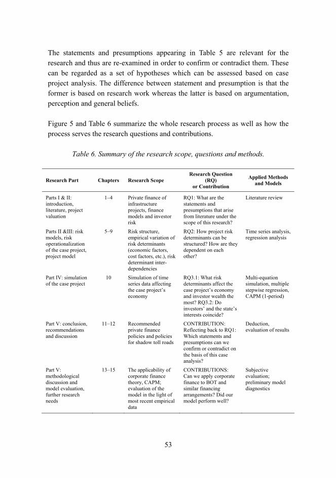
53

The statements and presumptions appearing in Table 5 are relevant for the research and thus are re-examined in order to confirm or contradict them. These can be regarded as a set of hypotheses which can be assessed based on case project analysis. The difference between statement and presumption is that the former is based on research work whereas the latter is based on argumentation, perception and general beliefs.

Figure 5 and Table 6 summarize the whole research process as well as how the process serves the research questions and contributions.

Table 6. Summary of the research scope, questions and methods.

Research Part Chapters Research Scope Research Question

(RQ) or Contribution

Applied Methods and Models

Parts I & II: introduction, literature, project valuation

1�4 Private finance of infrastructure projects, finance models and investor risk

RQ1: What are the statements and presumptions that arise from literature under the scope of this research?

Literature review

Parts II &III: risk models, risk operationalization of the case project, project model

5�9 Risk structure, empirical variation of risk determinants (economic factors, cost factors, etc.), risk determinant inter-dependencies

RQ2: How project risk determinants can be structured? How are they dependent on each other?

Time series analysis, regression analysis

Part IV: simulation of the case project

10 Simulation of time series data affecting the case project�s economy

RQ3.1: What risk determinants affect the case project�s economy and investor wealth the most? RQ3.2: Do investors� and the state�s interests coincide?

Multi-equation simulation, multiple stepwise regression, CAPM (1-period)

Part V: conclusion, recommendations and discussion

11�12 Recommended private finance policies and policies for shadow toll roads

CONTRIBUTION: Reflecting back to RQ1: Which statements and presumptions can we confirm or contradict on the basis of this case analysis?

Deduction, evaluation of results

Part V: methodological discussion and model evaluation, further research needs

13�15 The applicability of corporate finance theory, CAPM; evaluation of the model in the light of most recent empirical data

CONTRIBUTIONS: Can we apply corporate finance to BOT and similar financing arrangements? Did our model perform well?

Subjective evaluation; preliminary model diagnostics

54

PART II & III:

Project model-consisting of

several sub-models

PART I:

Theory-privatization of assets

-private finance

PART IV:

Simulationof the case

project

PART IV:

Outcomes & analysisof project economy

-project company & investors-the state

Empirical data analysis-linear regression

-descriptive statisticsLiterature review

Simulation-autoregressive,

multi-equation simulationof the case project using

the project model

Multiple regression

RQ1:Statements and presumptions

on the use and usabilityof private/project finance in

infrastructure projects

RQ2: Project ModelRQ2.1: Model structure

RQ2.2 & 2.3: Risk determinants,risk relationships and causality

RQ3: Economic performanceof the case project

RQ3.1: Determinants of performanceRQ3.2: Conflicting/coinciding

interests of stakeholders

Met

hodo

logi

cal

laye

rR

esea

rch

proc

ess

laye

r

Res

earc

h qu

estio

ns&

con

tribu

tion

laye

r Confirmation or contradiction of statements & presumptions

PART V:Model

diagnostics &evaluation ofresults andcontribution

Implications for-infrastructure finance policy & infrastructure management

-contractual strategiesFurther research needs

Is private finance applicable,in what terms and what are the risks?

Figure 5. Summary of the research process � methodological, research process and contribution layers.

55

3. Data and methods

3.1 Data sources

The primary source of time series data for road operating and construction is the Finnish Road Administration�s (Finnra) production statistics (Finnish Road Administration 1996a) which includes financial inputs to road construction and maintenance. The problem with this source is that it contains only national and regional data the latter being the most detailed level available concerning documented historical maintenance costs for 1981�1995. Costs on maintenance area level9 would perhaps give more detailed information on the costs of operations but this data is available only for a shorter period of time, i.e. 1991�1995. When ex post statistical data was not available or did not meet the requirements, Finnra�s own experts� estimates which were made for the case project were used.

For re-paving works as part of maintenance package the primary sources of information were Finnra�s pavement statistics (Finnish Road Administration 1993; 1996b) which cover contract prices and unit prices.

Some Finnra statistics include only internal input prices which may differ from market prices. This is especially true with winter maintenance costs as winter-time maintenance operations were then done mainly by Finnra�s own organisation. When it comes to construction and paving works prices, Finnra�s statistics reflect reasonably well against market prices since most of these works are done by contracting through competitive bidding. Since government agencies do not pay value added tax (VAT), the prices are excluding VAT.

There is a question when estimating the risk of operating costs using regional data: is regional data comparable to road specific data, i.e. how much should be

9 Every road region is divided to several maintenance areas. E.g. Uusimaa region contained 15 maintenance areas in 1995. Like in any organisation, the discussions with various Finnra personnel brought out the fact that behaviour of maintenance units include elements of �gamesmanship�. Gamesmanship is a pattern of behaviour of managers at different levels when these managers try to manipulate accounting numbers in favour to their own personal or organisational goals. In public sector this means allocating costs to activities where cost limits are not that strict and utilising the allowed budget to the maximum. See e.g. Euske (1984, pp. 71�73).

56

relied on aggregate data? The case project is only one stretch of motorway, and the task is to operationalize the operating cost risk of this project on the basis of regional information on past operating costs. Clearly, it is not self-evident that the information available is suitable for this purpose. The regional data did not identify any differences between road categories except for asphalt pavement roads and gravel roads. Road-specific data simply does not exist and it was not possible to carry out road-specific in-situ studies gathering cost data. Recently, the area-wise maintenance contracts that Finnra has adopted have changed the bidding and pricing strategies of maintenance contractors and thus some market prices have surely changed. As a result, there is also a discontinuity in maintenance cost data because of this.

The interest rates time series were available through public statistics (Statistics Finland, Bank of Finland) and posed no interpretation or applicability problems.

For traffic demand the time series of aggregate demand was available from the statistics of Finnra and project-specific demand through Finnra�s regionally maintained road and traffic data bases.

3.2 Methods

To assess the volatility of time series the ex post cost data was gathered and typical statistical ratios (mean, variation) were calculated. The prerequisites for this method are reliable and detailed ex post data records. Project-specific cost data was based on Finnra�s expert estimates, but the volatility attached to these items was based on relative variation derived from historical data.

The inter-dependence of variables is one of the key issues. For example, it is generally known that inflation and real interest rates are negatively correlated (see e.g. Lipsey & Chrystal 1995, pp. 513�515). Also it is reasonable to assume that general price changes of civil engineering works (the corresponding cost index) are correlated with road maintenance costs. These relationships (with uncertainty related to their regression parameters) have been used in the case project model construction.

57

The methodological approach for this research is the following:

1. In the first part there is a review of literature, the theoretical framework and the scope is set (Chapters 1 and 2). Also the basic tools of corporate finance and project valuation are briefly introduced (Chapter 4). The data sources and methodologies are discussed and described in Chapter 3. The theory of risk is discussed and the risk structure model is synthesized (Chapter 5).

2. The ex post data of each variable is shortly described and analysed for the use of specified models (Chapter 6). The description and analysis includes: i) evaluation of the time series available and used in this research; ii) the contract terms for the case project as far as they are known and not regarded as confidential; if confidential, the available information from tender documents or oral information from key people is used; iii) evaluation of the nature and behaviour (stochastic, stationary, contingency, variability) of variable in question.

3. The research continues with the analysis of inter-dependencies of selected variables with the help of multiple regression (Chapter 7); the inter-dependencies are used to build a multi-equation simulation model of the project framework. Similar simulation models are described by Pindyck and Rubinfeld (1991, p. 287). This model is used to research the behaviour of the case project in plausible future states of the world. STATISTICA® software is used to perform the regressions.

4. The research completes the project model on the basis of financial and investment theory. This model can additionally be regarded as an a priori decision support model for the case project and as such contributes to generic private financed projects� decision tools. The simulation software used is iThink® which allows multi-equation simulation combined with statistical distributions. Regression relationships provided by earlier research steps are used in the simulation. Some of the relations are later relaxed so that recent data is used as a starting point. However, the main modelling is done based on data series that ends in year 1996, which is the decision making point for project investors. This part is in Chapter 8.

58

5. In Chapter 10, the simulations that are performed provide results for statistical and structural analysis of the project. Simulations are carried out in two ways. First the whole network of interdependencies are let to vary according to empirical distributions (the distributions of regression variables) so that different possible outcomes are produced but maintaining the weak relationships between variables (endogenous and exogenous) of the project model. Similar approaches to generate observations by simulation are used in finance and economics literature � for Finnish examples, see e.g. Salmi and Virtanen (1997; 1995). These outcomes are then further analysed with the aid of multiple regression in seeking relevant critical factors. For example, the insolvency analysis is performed so that multiple cash reserve outcomes are simulated with the simulation model and then the key determinants of insolvency are sought by multiple regression.

6. Finally, the results are discussed, analysed and concluded and future research needs are identified. This part is the researcher�s subjective interpretation of the results and dealt with in Chapters 11�14.

Simulation was selected as the primary method because of the complexity of the analytical solutions. Furthermore, the lack of empirical observations compelled to simulating observations in order to test probabilistic models. Thus, this research also falls into the category of systems analysis, the system being the case project and the observations being the results and outcomes of simulations of the project (see e.g. McMillan & Gonzales 1973, pp. 20�25). The project model is a multi-equation simulation model as defined by Pindyck and Rubinfeld (1991, p. 287). The typical field for these types of models has been econometrics, but have been more and more widely adopted for e.g. corporate financial planning and engineering (Pindyck & Rubinfeld 1991, pp. 360�361).

59

PART II: PROJECT VALUATION AND PROJECT RISK

In this section, the concept of risk is presented in the framework of financial theory. Then, the relevant project cash flows are identified as it is their volatility that builds the risk for the project. The project cash flows are studied in detail as to how they form the value of the project. This is followed by brief introduction of risk models and the approach used by financial theory is categorized. Also the different typologies of risks are introduced based on literature concentrating particularly on civil engineering and construction projects. Starting from the cash flows and ending up to risk models, a synthesis is presented in the form of project�s risk structure model.

The end result of Part II are thus the cash flow model and the risk structure model, the former based on financial theory and Capital Asset Pricing Model, the latter based on cash flow model and literature on risk. The private investors� risk dominates the view taken.

This section gives preliminary answers (conceptual models) to the following second set of research questions:

RQ2: What kind of project model can be constructed for the analysis of privately financed infrastructure project?



61

4. Project valuation

4.1 Project valuation using CAPM

The net present value (NPV) rule of the investment is:

( )∑=

−⎟⎟⎠

⎞⎜⎜⎝

⎛

+=

n

tt

p

t Ir

FCFNPV0

01 (Eq.4-1)

where

NPV = net present value of the project FCFt = free cash flow in period t rp = cost of capital and required return on project n = number of periods I0 = initial investment in project.

Consistency in financial theory requires that the discounted free cash flows net of initial investment equal the net present value of the project which represents the increase of wealth of project investors. The required return is adjusted using e.g. Capital Asset Pricing Model (Sharpe 1963; Sharpe 1964; Treynor 1961) on the basis of how risky the cash flows are. CAPM was developed for principally valuation of stock market securities but has been used further to evaluate individual projects (see e.g. Brealey & Myers 1991, p. 206) and physical investments (see e.g. Bogue & Roll 1974; Dias & Ioannou 1995). A review of empirical tests on CAPM can be found in Copeland and Weston (1988, pp. 212�217).

Using CAPM as the measure of project return under uncertainty one needs to define 1) a risk free interest rate for a risk-free asset, 2) the risk, that is, the variance, of all marketable assets, i.e. market portfolio variance, 3) the return on market portfolio, and 4) the risk (variance) of risky asset in question. The CAPM is written as a function of expected return on project rp

( ) ( )[ ] pfmfp rrErrE β−+= (Eq.4-2)

62

where

rf = risk-free rate of interest; usually the empirical values are government/state bond interest rates

E(rm) = expected rate of return of market portfolio; e.g. a fully diversified investment in stock exchange securities

( )( ) 2

2,,

m

mp

m

mpp rVar

rrCovσ

σβ == (Eq.4-3)

βp = covariance between project return and market portfolio return divided by variance of market return; if β >1 the project return is sensitive to market conditions and thus more risky, if β <1 the project is less risky than market portfolio; E(rm) � rf is the risk premium for market portfolio as the portfolio is more risky than a risk-free asset.

In order to be profitable i.e. to have a positive NPV the project must satisfy the following condition under the assumption of market equilibrium (a tilde [~] symbolizes the uncertain value of variable):

( )( )

( )( )[ ] pfmf

p

p

p

rrErVE

rEVE

Iβ−++

=+

≤ ~1

~

~1

~11

0 (Eq.4-4)

where

Vp1 = the (uncertain) end-of-period value of project; one-period project I0 = cost of initial investment, that is, the value of project at the start.

The CAPM can be used to determine the present value of the project as done by Dias and Ioannou (1995).

63

The project risk, project beta, is

( )( ) fm

fpp rrE

rrE−

−= ~

~β (Eq.4-5)

As the project risk consists of many interrelated or individual variables project risk in some cases may have to be divided into its critical cash flow components (Copeland & Weston 1988, pp. 414�416). For the case project of this study, this approach was used in Leviäkangas (1998), yielding to almost zero beta, βp≈0.

4.2 Project cash flow model and stakeholder values

To start with, the following symbols are used:

Rev = revenues of the project company; in the case project these are the shadow toll revenues paid by the state to the project company

Ope = operating expenses of the project company; these are mainly all-year-round road maintenance costs

C = construction cost, i.e. the expenses of building the road

Tax = corporate taxes paid by the project company

E = equity capital invested in the project company

D = debt capital raised by the project company

iD = interest on debt capital

A = amortisation of debt

Dep = depreciation of the road asset

Tc = corporate tax rate.

We assume only corporate tax.

The risky cash flows of the project company and the risks of different parties like equity investors, debt investors, and the state, are later described as the project model is developed. However, a preliminary model is shown in Figure 6.

64

The predecessor of this example is from Lawson and Stark (1975, p. 23). In Figure 6 the case project structure has already been assumed so that e.g. the state pays shadow toll to the project company.

The simplified description of cash flows of different parties involved (excluding project company�s personnel and suppliers) is shown in the cash flow statement in Table 7. It is assumed that the project company distributes immediately all the net cash flow earned to shareholders as dividends. This is a reasonable assumption since the whole idea of the project is to generate adequate and as-early-as-possible cash stream to investors.

Project companyDebtinvestors

Equityinvestors

State

Subcontractors & suppliers

Operating personnel & equipment

Long and mediumterm debt

Interest andamortisation

Shadow tolls

Corporatetaxes

Operating cost

Returns on equityEquity

Figure 6. A simplified model of project cash flows.

Table 7 depicts the cash flows of a project company and its framework as shown in Figure 6 and forms the central piece of the entire analysis.

65

Table 7. Project cash flows to different stakeholders.

Equity investors

Debt investors

Project company The state Contractors &

suppliers Notes &

explanations

-E +E Equity investors invest E in the project company

-D +D Debt investors invest D

-C +C Project company constructs the road at expense C

+Rev -Rev Project company receives shadow tolls from the state

-Ope +Ope

Project company pays contractors for the operating (e.g. maintenance)

+iD -iD Project company pays interest on debt

+A -A Project company amortizes the debt

-Tax +Tax

=Tc(Rev-C-Ope-Dep-iD)

Corporate taxes after expenses, depreciation* and interest

+[(1-Tc)(Rev-C-Ope)+TcDep+Tc

iD]

-[(1-Tc)(Rev-C-Ope)+TcDep+T

ciD]

The surplus cash flow available for shareholders, paid by the project company**

* Depreciation (Dep) equals the cost of depreciated asset (C) ** The available surplus for investors after their capital outlays = (1 -Tc)(Rev � C � Ope � Dep � iD) = Rev � C � Ope � Tax = Free cash flow (FCF)

The free cash flow to investors (FCF) is the measure of wealth increase for them. This surplus is available for investors after their initial capital outlays (E, D). All the remaining analysis is based on this concept. To open the calculus of the table we formulate the free cash flow for shareholders which is after-tax net cash flow plus tax advantages from depreciation and interest payments

66

FCF = (1 -Tc)(Rev � C � Ope) + TcDep + TciD = Rev � C � Ope � Tc(Rev � C � Ope � Dep � iD) = Rev � C � Ope � Tax

because taxes paid by project company must be

Tax = Tc(Rev � C � Ope � Dep � iD)

The total cash flows for a single project company build up from total cash flows to equity holders, defined as

TCFE = (Rev � Ope � C � Tax � iD � A) � E (Eq.4-6)

and the total cash flows to debtholders

TCFD = (iD + A) � D (Eq.4-7)

Summing these two form the total cash flows of the single-project company

TCFE + TCFD = Rev � Ope � C � Tax � (E + D) = FCF � (E + D) (Eq.4-8)

which states that the incremental value produced by the single-project company to its owners is the free cash flow minus the initial capital outlays of equity and debt. Net present value of project investors� investment (NPV_PI) follows when their invested capital is subtracted from present value of project company�s cash flows.

NPV_PI = FCF � E � D (Eq.4-9)

The market value of the project company is the present value of free cash flows, i.e. the initial capital outlays plus the incremental value:

Vp = FCF = E + D + NPV_PI (Eq.4-10)

The market value of debt is the initial debt outlay plus the incremental available to debtholders

Dm = D + TCFD = D + (iD + A) � D = iD + A (Eq.4-11)

67

The market value of equity is the initial equity outlay plus the incremental available to equity holders

Em = E + TCFE = E + (Rev � Ope � C � Tax � iD � A) � E = FCF � iD � A = FCF � Dm (Eq.4-12)

The market value of the single-project company may be written also as

Vp = E + D + NPV_PI = (Em � TCFE) + (Dm � TCFD) + (TCFE + TCFD) = Em + Dm

(Eq.4-13)

The returns on project, debt and equity are consequently

ppmm

p rDE

PINPVDE

FCFDE

PINPVDEDE

VDEDER +=

++=

+=

+++

=+

=++

= 1_1_ (Eq.4-14)

where Rp and rp represent the end-of period returns on compounded basis.

Assuming that equity and debt investor outlays in the beginning of the project are equal to investment outlay in Eq.4-4 and that end-of-period project values in Eq.4-13 and Eq.4-4 represent the same things, i.e.

( ) ( ) pppp rrEVVEDEI ==+= ~and~and 10 (Eq.4-15)

results in consistency with basic CAPM-based project valuation:

( ) ( )p

mmppp r

DEDE

DEV

IVE

rE +=++

=+

==+ 1~

~10

1 (Eq.4-16)

rp being determined by Eq.4-2.

68

4.3 Cost of capital

Determining the appropriate discounting rate for project cash flows includes the calculation of weighed average cost of capital (WACC). It is possible to estimate WACC by CAPM in a world of corporate taxes only using the following relationships (Copeland & Weston 1988, p. 456):

( )[ ]( )[ ]

( )p

mDc

p

mE

DfmfD

EfmfE

VDrT

VErWACC

rrErr

rrErr

−+=

−+=

−+=

1

β

β

(Eq.4-17a, 4-17b, 4-17c)

where

rE and rD are the risk-adjusted required returns on equity and debt

βΕ and βD are the covariances between return on equity/debt and market return divided by the variance of market return

Em and Dm are the market values of equity and debt and their sum Vp is the total market value of the project company

Rf is the risk-free rate and E(rm ) the expected return on market.

The cost of capital tends to decrease as the debt financing increases due to tax advantage of leverage.

The estimation of betas is simple using historical data. However, in a single-project company the use of WACC is problematic: the market values of debt and equity are needed to set weights for the WACC formula but the market values are not necessarily available if a) the project is not quoted by the market and b) the market value of the project is dependent on future cash flows but the cash flows cannot be discounted properly without WACC (which in turn needs market value weights). A simple method would be to use face value weights, though the textbooks do not recommend that. However, this should not result in an excessively large error, due to the following reasons:

− The equity needed to finance the project is mostly used to cover cash outlays in the beginning of the period (e.g. construction costs, purchase of equipment,

69

etc.) when cash inflows do not yet occur; thus, the equity invested reflects the market value because it can be considered to be quite close to the replacement (= repurchase or reconstruction) value of the project (Copeland & Weston 1988, pp. 446�447).

− The face value of debt in the beginning of the project should not differ too much from the market value of debt, either, and book values are commonly used for debt unless market values are available.

− The error of using book values in this kind of project is usually in the same direction with both equity and debt, i.e. they both are probably too low compared to market values given that the project is profitable and has a positive NPV.

The implication is that the risks of the project, i.e. project beta but also betas of equity and debt, change as the leverage changes. Copeland and Weston (1988, p. 471) present the following equations based on work by Hsia (1981) where the analogy between option pricing theory and risky debt is combined10:

( ) ( ) ( )

( )( )

⎟⎟⎠

⎞⎜⎜⎝

⎛−=

−−+=

⎥⎦

⎤⎢⎣

⎡−−+−=

p

mcE

m

mcDEEE

m

pfEfcD

VDTWACC

EDTkk

DV

dNrrTk

1

1

1 1

ρ

ρρ

ρ

(Eq.4-18a, 4-18b, 4-18c)

where

kD and kE are cost of debt and equity capital Tc is the corporate tax rate and rf is the risk-free rate of interest ρΕ is the cost of capital for an all-equity financed project N(d1) is the cumulative normal probability of the unit normal variate d1, expressed as:

10 Risky corporate debt is equal to default-free debt (i.e. no risk) minus a put option (the alternative that debtholders receive less than promised in case of default) (Hsia 1981; Copeland & Weston 1988, pp. 464�471).

70

tt

trDV

df

m

p

σσ 2

1ln

1 +×+⎟

⎠

⎞⎜⎝

⎛

= (Eq.4-19)

t is the time maturity for debt D and σ2 is the variance of return on project company�s assets, i.e. return on project.

Again the determination of costs of capital requires market values which are not available for a non-quoted single-project company; the cash flows can be used to approximate market values but the cost of capital discounted cash flows need in turn the market value weights which leads to the same problem as previously. The variance of return on project has to be estimated on the basis of historical data. However, using the initial capital outlays of debt and equity as weights and estimating the variance of project returns e.g. by using historical traffic development it is possible to approximate cost of capital with different capital structures.

71

5. Risk structure model

5.1 Different perspectives to risk and classifications of risk models

In this section, the risk structure for the case project is constructed. The structure describes the determinants that are usually in financial theory captured in one term, i.e. the discounting rate; the risk is operationalized with risk adjusting multiplier, the beta. However, behind the one term and multiplier there are numerous factors that build up the project�s aggregate risk. These factors, determinants, are the ones which are structured and described in the following. Before directing to risk factors and risk classifications, it is appropriate to discuss very briefly various risk models and their underlying theoretical premises. Shoemaker (1980, pp. 28�44) classifies risk models according to Figure 7.

Capital Asset Pricing Model (CAPM) is a mean-variance risk model based on Markowitz�s portfolio theory (Markowitz 1959) and expected utility theory.

It is also in place, in the beginning, to distinguish between speculative and pure risks as done by Doherty (1985, p. 3). Speculative risk offer also the possibility of gain but pure risk have only losses to offer. Most risks in financing context are speculative risks. Doherty takes the financial approach to the definition of risk and states:

�Thus risk relates to the underlying variability in some relevant value; measures of risk are mathematical conventions to summarize the pattern and extent of such spread.�

72

Figure 7. Classification scheme for descriptive risk models (Shoemaker 1980).

Risks of the project vary according to perspectives taken by each party involved. Sponsors (owners, equity investors), lenders, contractors and suppliers, government, and customers have their own risk perspective and thus differing risks related to the project. Bond and Carter (1994, pp. 15�24) provide a generic risk profile for privately financed infrastructure projects as follows:

− Commercial risks, consisting of a) project-specific risks; developing and constructing the project, operating and maintaining the assets, and finding the market; b) broader economic environment risks, including such as interest rate changes, inflation, currency risk and international price movements of raw materials and energy inputs.

− Non-commercial or policy risk, consisting c) project-specific policy risks such as expropriation, changes in the regulatory regime, and failure of the government or its public enterprises to meet contractual obligations; and d) political risk which includes events such as war or civil disturbance.

Furthermore, Bond and Carter identify the time perspectives of the project with different risk profiles and financing requirements. Development phase includes a very high risk; this is why equity capital is usually used. Construction and start-up phase also include a high risk and require large volumes of capital � debt and equity and all their variants are deployed. In the operational phase the risks are lower but refinancing may still be required.

Expected utility theory Expected utility models with probability transformations Mean-risk models Additive models

Subjective probabilities

Subjective weights

Disjunctive models

Conjunctive models

Additive-difference models

Dominance models

Lexicographic models

Elimination-by-aspects models Comparisons within attributes

Comparisons against some standard

Non-Holistic

Holistic

Decision Models

(sequential eliminations)

Comparisons across attributes

73

Also Griffith-Jones (1993, p. 22) identifies these three phases of the project and risks they contain. She formulates a typology of risks as shown in Table 8.

Table 8. A typology of risks (Griffith-Jones 1993, p. 22).

Project phase Risks

Promotion and preparation Failure of feasibility study Unsuccessful bid Planning/environmental consents delayed or not

obtained; other legislative difficulties Construction Delays and cost overruns attributable to contractors;

technical non- or underperformance Delays due to force majeure �Policy� risks; e.g. non-completion of associated

infrastructure, changed environmental regulations, transport policy development

Inflation / Currency risk / Interest rates Operating Technical difficulties Revenue shortfalls and excess costs for commercial reasons

(low levels of traffic, changes in input prices, etc.) Revenue shortfalls or cost overruns due to �policy�

changes (competing infrastructure, environmental regulations, etc.)

In Kangari�s (1995) report of ASCE (American Society of Civil Engineers) questionnaire concerning US contractors� risk management and priorities in 1993, the results were according to Table 9. It is clearly seen that the construction phase alone is divided into numerous technical and financial risks. However, as Kangari reports, it should be emphasized that risk management trends vary over time � as world changes, so do risks. Furthermore, Table 9 mainly describes conventional construction contracts while privately financed contracts include a special emphasis on the financial issues. Hence, they are certainly more complex in terms of risk management.

In a BOT-type of project, there are some risks in Table 9 which would intuitively seem more important than others. Financial failures, inflation, changes in

74

government regulations, and any risk that affects either to construction cost or the revenue stream of the project are of more significance than in an ordinary type of project which excludes operating phase and long-term capital financing.

Redhead and Hughes (1988, pp. 3�8) analyse financial risks and subdivide foreign exchange rate risk further to transaction, translation and economic exposure. Transaction exposure is the possibility of gains and losses from the direct effects of rate movements on anticipated cash flows. Translation exposure is also known as accounting or balance sheet exposure which arises from mismatch between assets and liabilities in foreign currencies or mismatch between valuation principles. Economic exposure is the exposure to the effects of exchange rate movements on the economic environment of the company such that the volume of turnover is affected or the prices of its domestic inputs or outputs change relative to other prices within the domestic economy.

Table 9. Risks and their importance; US contractors� view in 1993 (Kangari 1995).

Risk Description Importance (1�10), average of replies

Safety 8.3 Quality of work 8.2 Defective design 8.0 Labour and equipment productivity 7.6 Delayed payment on contract 7.5 Contractor competence 7.5 Financial failure � any party 7.3 Changes in work 6.9 Differing site conditions 6.9 Contract-delay resolution 6.8 Indemnification and hold harmless 6.5 Labour, equipment and raw material availability

6.4

Change-order negotiations 6.4 Third-party delays 6.2 Actual quantities of work 5.8 Site access / right of way 5.6 Labour disputes 5.5 Defective materials 5.1 Inflation (lump-sum or unit price contracts) 4.7 Permits and ordinances 4.7 Defensive engineering 4.6 Acts of God 4.4 Changes in government regulations 4.1

75

Ren (1994) brings more dimensions to project risk management. He introduces the concept of �risk lifecycle� which means that the time property of risk, i.e. start and end time of risk occurrence is also taken into account. This approach relates to risk profiles listed by Bond and Carter. The earlier the project phase, the more risk occurrences are there ahead. Assigning risk probability distributions with cash flow effects makes up the risk profile of the project. Ren also lists the basic patterns of risk relationships. Independence of risk means that it does not affect any other risk in the system. Dependence is naturally the opposite situation where one risk occurrence will affect the probability of another occurrence (if A happens, then probably B will happen). In the parallel risk relationship more than one risk (A, B, C...) together will affect one or more other risks (a, b, c...) and in the series situation all the risks (A, B, C...) must happen if risks (a, b, c...) are to happen. It is easy to see that Ren�s method is important from the cash-management and liquidity perspective of the project. The risk profile points out when the risks of the project may occur and the risk relationships update the risk profile if risks are continuously monitored.

5.2 Synthesis � risk structure of a project

On the basis of the above discussion, the risks of the case project are attempted to classify in a meaningful way so that project risks may be quantified. In the end, all risks have a financial effect to the outcome of the enterprise.

Financial risks

The risks involved in a privately financed infrastructure capital investment project may be classified according to uncertainties that relate to either 1) receiving an expected benefit or cash flow, or 2) construction cost, costs of operating or financing costs of the facility. Some risks appear to be critical while others are more trivial. However, the organisational and contractual framework allocating the risks between parties involved determines the importance of each risk from different viewpoints. The risks may be listed according to their economical context as follows:

− construction cost risk; defective design, defective cost engineering, increases in input prices (inflation)

76

− interest rate risk; cost of debt capital

− foreign exchange rate risk in case of foreign investors

− operating cost risk; inflation

− demand risk; revenues from operation (from users of the service or as shadow charges from the government)

− risks related to technical implementation and operation of the project � e.g. time delays in construction or closing down the facility in case of accidents, etc. � which causes a disturbance to operating revenues even if demand factors remain unaltered.

These are the fundamental financial risks (in the end, technical risks always transform to financial risks) that can be transferred and allocated in various manners depending on the contractual arrangements applied in each case. Also equity holdings arrangements affect the behaviour and risks of different parties. For example, if project contractors and suppliers are also the equity investors of the project company, they have an incentive to perform their contracts economically and efficiently in order to guarantee a successful starting point for their investment, i.e. the project. Debt financiers are likewise interested in ensuring a successful implementation and operation of the project as they face the risk of loosing some of their investment in the case of bankruptcy.

Technical risks

In engineering projects technical risks are always present and form the most potential source of risks which then turn into financial risks. For the specific project in question, the following risks may be identified which in fact apply to any civil engineering project:

a) construction delays which delay the completion; this may be due to

− bad weather conditions − difficult or unexpected ground conditions − delays of subcontractors or suppliers − shortage of construction equipment or materials or special equipment related

to technical systems of the project

77

− shortage of human resources, i.e. skilled labour and management − accidents on the site − design or construction errors which have to be repaired − difficulties to put installed technical systems in operation

b) quality of works which may be due to

− insufficient quality control, poor workmanship or materials quality − design, engineering and construction errors.

Other risks

To this group, one can include political and regulative risks that are mainly caused by national or local government actions (e.g. corporate tax, fuel tax, environmental taxes, etc., or legislative actions, e.g. traffic restrictions, emission standards, etc.). Also force majeure risks such as catastrophes, wars, strikes, acts of terror, etc, fall into this category. These risks exist, but in normal conditions they are disregarded unless the project itself is especially vulnerable � e.g. nuclear power plants, large dams, and like.

As was previously discussed, the risks of the project are financial risks and technical risks related to time and quality. Cost, time and quality are and have always been the fundamental project management issues. The risk structure may be illustrated as a tree-like hierarchy (Figure 8) where also causal relations of factors are shown. Time delays in construction phase, for instance, will inevitably lead to disturbances in revenues. All the technical and other risks have ultimately a financial impact on the project�s economy.

In Figure 8, the different phases for different risks overlap and sometimes it is difficult to assess in which phase of the project each risk should or could be identified and when these risks eventually could realize. The risk structure model can be utilized in various types of projects to assist risk identification process and risk assessment.

78

Operating costs

Demand

Construction cost

Disturbances in revenues

Interest & exchange rates

Economy-wide

Project-specific

Time delays

Quality of works

Operating problems

Government policy

Force majeur

Financialrisks

Technicalrisks

Otherrisks

Proj

ect r

isk

F = feasibility study phaseC = construction phaseO = operating phase

F/C/O

C

C

O

F/C/O

F/C/O

F/O

F/C

O

O

Figure 8. Risk structure of a privately financed civil engineering project (modified from Leviäkangas 1998).

79

PART III: PROJECT MODEL SPECIFICATION BASED ON EMPIRICAL

DATA

In this part, the risk determinants identified in the risk structure model and thus affecting the cash flows of the project are described and their correlations with each other are analyzed. This is done according to risk theory stating that in many occasions risks are not independent from each other. The classification of risks follows precisely the classification presented in the risk structure model in Figure 5 (economy-wide, project specific). As a result, the project framework model is provided (Figure 20) that conceptually ties the variables to the project cash flows and shows how the variables are dependent on each other. This way, the project framework model goes further in detail than the risk structure model. Empirical volatility of variables represent the ex post risks, or rather empirical factors contributing to risk. Project framework model is also presented mathematically as a multi-equation model.

Full project model ties everything together at project cash flow level. The full model incorporates a macro-economic scenario module, without which the simulation would not be possible, as all simulations are essentially artificial states of the world which may vary depending on the model specification. The full project model allows cash flow and value analysis of the project following the principles of financial theory. Different scenarios aid in assessing the volatility of cash flows and thus define the risk (volatility) of the project. Again, the main emphasis is on investors� risk.

80

This section begins with assessing the volatility of different cost and revenue items and their determinants: interest rates, traffic demand, construction cost, operating cost and some specific issues related to disturbances in operation of the road. Then, the interdependencies are analyzed based on empirical data resulting in the project framework model. Finally, after specifying the economic scenarios model, the full project model is specified. The model starts with economic growth scenarios, generates interest rate and traffic demand (both national and project level) scenarios and thereon calculates the project cash flows in each simulated scenario.

The project beta is estimated mainly based on literature and earlier related studies. Beta is needed later to calculate project company�s cost of capital. Beta can also be regarded as a single-figure yardstick to assess project risk with relation to any other market investments.

This section provides more detailed answers to the second set of research questions:





81

6. Empirical volatility of economy-wide and project-specific variables

6.1 Interest rates

Interest rate changes constitute usually a major risk in investment projects. In the case project, the interest rate risk is borne totally by the contractor. The interest rate risk is mainly concerning debt capital which is usually granted with market-based variable interest rates added with appropriate premiums. The concessionaire/contractor was eligible to seek loans from European Investment Bank (EIB). EIB grants loans for prospective projects maximum 50% of the investment cost with maximum 25 years pay-back period. It is possible to have loans with first four years without interest. The rest of the debt capital is raised from domestic or international capital markets. The loans granted by EIB are probably less risky from the viewpoint of the borrower than ordinary domestic bank loans. However, it was assumed that prospective debt is raised from national institutions.

In practice, concessionaires of BOT-type projects hedge themselves against interest rate risk, but hedging of course has to be paid for. The costs of hedging should therefore be included in the bidding price. In order to assess the significance of interest rate risk, this study is not assuming any a priori hedging plans, but attempts to show the magnitude of interest rate risk.

According to statistics of Bank of Finland, domestic loans granted by Finnish commercial banks for firms during 1985�1995 cost approximately between 7 and 14% according to Table 10. The market rate of interest (12-months Helibor) varied between 6�15%. The 12-month Helibor rate is assumed to describe well enough the interest rate volatility of risky debt contracts with long maturity. Various Helibor rates are commonly used by Finnish banks added with negotiable premiums.

82

Table 10. Time series of interest rates (Bank of Finland 1986�1996; Nordiska Ministerådet 1996).

Year 12-month Helibor* (%)

Average lending rate of new loans for firms

(%)

1995 6.34 7.30 1994 6.33 7.13 1993 7.47 9.40 1992 12.96 13.32 1991 12.53 13.40 1990 14.39 13.33 1989 12.72 11.58 1988 10.50 10.50 1987 10.40 10.01 1986 na** 9.76 1985 na 10.62 1984 na na 1983 na na

* Average daily observations ** 12-month Helibor was quoted starting from November 1987

6.2 Traffic demand

Historical data of traffic demand is available at all three levels: national, regional and even project-specific data. The last mentioned is available only partly, though. The past data of national and regional traffic demand, i.e. vehicle kilometres of travel, are shown in Figure 9. Both national and regional demands have been growing steadily until the economic down-turn in the shift of 1990�s. The growth rates are supposed to have a long-term stationary average. However, regional traffic demand started growing earlier than national. The natural explanation is that the up-turn in economy usually starts from the capital region of Uusimaa and the rest of the country follows slightly lagged. This is simply because of concentration of economic activity.

Since the demand for traffic is so much dependent on general macroeconomic and demographic development the quantification of demand risk is really betting on other factors, mainly economic growth. Therefore, in order to focus on

83

correct risk factors, concentrating only on demand variations as such is not relevant. The next chapter deals in more detail with different risk parameters’ association with each other.

The concession contract stated that traffic demand risk is borne by the project company.

Figure 9. National, regional (Uusimaa region) and road-specific changes of VKT estimates for 1980–1994.

6.3 Construction cost risk

Concession contract terms

The construction cost risk is borne by the project company unless it can be shown that the cost increase due to the owner’s actions or erroneous information. The paving works of the new carriage-way are included in the investment part of the contract. In the actual contract, the investment part consisted of fixed payments of substantial sums during the construction period. These payments

84

were supposed to cover at least part of the construction cost. Toll payments would start as soon as the new carriage way was opened for traffic. The exact contract terms were confidential.

Expected cost

The initial cost estimate in 1995 price level for the detailed engineering and construction of the project is between 550�590 million FIM, VAT excluded. Therefore the expected amount of investment may be estimated as 570 million FIM. The band of the cost estimate seems quite narrow: only about ±3.5% of the total investment cost. According to Finnra statistics the unit cost (million FIM / km) of improving a semi-motorway to a full motorway varies significantly depending on the surrounding conditions and the scale of construction. Table 11 shows the variation of the unit costs (Finnish Road Administration 1996c). The costs include all other construction works needed due to the new project, i.e. bridges, other roads, game fences, noise barriers, etc.

Table 11. Unit costs of up-dating a semi-motorway to a motorway; million FIM / km, 1995 prices; VAT excluded.

Favourable conditions

Average conditions

Difficult conditions

Capital region 3.8 5.8 10.0

Urban areas 3.5 5.5 8.5

Rural areas 3.0 4.0 6.0

The initial cost estimate for the case project yielded to 8.3 million FIM / km which is close to unit cost of urban area in difficult conditions (8.5 million FIM / km). The unit cost would vary between 8.0�8.6 million FIM / km corresponding to the total cost estimate boundaries.

Cost estimating process and assessing accuracy of construction cost estimates

The cost estimating process, however, is not discrete in nature but rather continuous. As the economic environment and engineering conditions change

85

during the planning and construction processes the investment cost estimate is also continuously changing. Therefore, it is difficult to compare �estimated� and �realized� costs as there is no universally accepted specific cross-section of time where a final �estimate� is made and when �realized� costs can be measured. From the contractor�s point of view, one critical point of time is bidding. When bid is made, the contractor accepts a risk of making an error. If the bid is too high the contract is not won and if the bid is too low, the project will result economic loss.

In the case project the bidding was extremely difficult for contractors or concessionaires since the bidding had to be done in the preliminary phase of engineering which made the cost estimation alone more difficult than normal. Obviously, this meant increased risk for the bidders. The construction cost risk in the case project consisted of two major components:

1. Risk of defective design (e.g. not taking enough into account difficult ground conditions) and erroneous quantity estimation (not including enough materials or labour input in the estimation)

2. Risk of input and commodity price increases during the detailed engineering and construction phases (e.g. wage increases, materials prices, etc.).

In order to measure the former, empirical analysis would have to be carried out. Extensive studies of this type have not been done in Finland, but some sources of data do exist. A cross-sectional analysis of Finnra�s investment projects was reported by Finnra Staff in 1991 (Finnish Road Administration 1992). The report showed that the original cost estimates that were prepared for the 1991 budget (the preparation took place in the spring of 1990) decreased in total by 4% compared to the final estimates in fiscal year 1991. However, these were not the real final estimates, except for those projects that were completed in 1991. So these estimates show the changes in estimates during a period little less than two years. The estimates are mostly based on preliminary engineering plan11 which is exactly the situation also in the case project.

11 Source: discussions with Finnra Staff experts. However, some projects are planned ahead of the typical schedule and their cost estimates might be based on more detailed engineering plans, but is virtually impossible to identify what planning stage is the basis of cost estimates without examining each project individually.

86

Ex post data on general cost variation

Good time series statistics are available for civil engineering works and road construction works. The road construction cost index is available only until 1993 and thereafter it is identical with civil engineering works cost index. The case project�s planned investment period was May 1997 � Autumn 2000. Since many decisions were to be made before the construction period started, it is reasonable to simplify that the period of interest is approximately 1997�2000, i.e. four full calendar years. Starting from year 1995 and going back to year 1980 there are thirteen 4-year periods which are also shown in Table 12. The index series (see also Figure 10) is constructed so that from 1991 to 1995 the index is civil engineering works cost index and before 1991 the index is road construction cost index. The two indexes do however, measure the same phenomenon.

In light of past history, the four-year construction period may be subjected to general price changes which annually may vary between -1.7%...+13.5%. This means that the extreme scenario would be a rise in prices of more than one third of the total cost, assuming 3�4 years construction period. It is justified to assume that contractors are aware of this risk, if the risks are within the vicinity in the economy. Radical price decreases have not occurred. The annual changes have declined at the beginning of 1990�s. The longer term average seems to be around 5%.

87

Table 12. Construction cost time series.

Year

Road & civil eng. works cost index* 1990 = 100

Annual change

(%)

4-year period

change (%)

4-year minimum

(%)

4-year maximum

(%)

4-year annual average

(%) 1995 103.8 2.2 3.6 -1.7 2.2 0.5 1994 101.6 1.8 -0.3 -1.7 1.9 0.4 1993 99.8 -0.4 -0.2 -1.7 5.7 1.4 1992 100.2 -1.7 5.9 -1.7 7.9 3.5 1991 101.9 1.9 16.2 1.9 7.9 5.3 1990 100.0 5.7 20.4 5.6 7.9 6.2 1989 94.6 7.9 20.5 2.1 7.9 5.3 1988 87.7 5.6 14.0 2.1 5.8 4.4 1987 83.1 5.8 12.7 2.1 5.8 4.4 1986 78.5 2.1 12.1 2.1 8.2 5.0 1985 76.9 4.3 18.9 4.3 8.2 6.3 1984 73.7 5.3 22.5 5.3 13.5 8.6 1983 70.0 8.2 32.0 7.5 13.5 9.7 1982 64.7 7.5 1981 60.2 13.5 1980 53.1 * From 1991 to 1995 civil engineering works cost index and before that road construction cost index. Starting from 1994 there was no separate road construction cost index.

Figure 10. Civil engineering works cost index (Hemmilä & Kankainen 1993 and direct information service from Statistics Finland 2006).

88

Project cost estimate variations

Finnra (Finnish Road Administration 1991) studied the cost estimate changes and found that for more than 100 MFIM projects, the cost estimates had changed between -12.9%...+30.4% from initial estimate made in spring 1989 to a revised or final estimate at the end of 1991. The general price changes had already been taken into account in this analysis. Finnra studied altogether 140 projects, out of which 18 were initially estimated to cost more than 100 MFIM. Out of these 18, the cost estimate changes of most (14) cases were between -10%...+10%. The overall impression is that the effect of cost engineering error for larger projects seems to be somewhere around -10%...+10%. Figure 11 shows that a rectangular distribution can be used as a proxy, extreme values being -10%-units and +10%-units.

Figure 11. Distribution of project cost estimate changes, large projects (>100 MFIM), n = 18.

It should be once again reminded that the data is from Finnra which does not necessarily reflect accurately the cost engineering practices of private contractors. Usually, private contractors are well acquainted with day’s market prices. It may also implicitly be assumed that in the case project, the bidders’

89

cost engineers will tend to adjust their estimates more on the �safe side� as they have no experience either from the projects of this kind (domestic bidders) or the Finnish operating environment (foreign bidders).

6.4 Operating costs

6.4.1 Contract terms and cost structure

Concession contract terms

The operating (= maintenance) costs are tied in civil engineering works cost index. Thus, the risk of increases in general price level is borne by the state. Exceptional winter conditions, additional or earlier-than-expected re-paving operations and the road-specific variation of operating cost risks are borne by the concessionaire. In the early versions of the contract draft the price of bitumen and salt had a special clause in the contract so that significant price increases of these items would have been compensated to the concessionaire. Due to the index clause of operating costs the previous special clauses were left out. In the forthcoming analysis it is assumed that index clause does not exist.

Cost structure

Operating costs of the case project may be divided as follows:

− Daily maintenance costs which include winter maintenance operations (snow removal, de-icing, sanding, cleaning, etc.) and summer time operations (road markings, vegetation removal, and other minor road surface maintenance works)

− Re-paving operations which have to be done periodically in some years� intervals

− Other major maintenance operations such as strengthening the base course if necessary, maintenance of bridges, constructing additional sewage if necessary, etc.

The first two items form three-quarters of the total operating cost of the project. The operations are divided according to Finnra standard coding system (Finnish

90

Road Administration 1990). The codes cover all the maintenance operations a motorway section requires during its first two or three decades after completion. The operations and corresponding codes are the following:

− Day-to-day winter maintenance which includes sub-operations (with sub-codes) such as snow-plough marking, snow removal, mechanical ice removal, sanding, de-icing, winter-time drainage maintenance, weather monitoring activities

− Maintenance of asphalt pavement roads which includes pavement maintenance, re-paving, small repairs of subgrade structures, drainage system maintenance

− Traffic control and traffic management services which consists of road markings, signing maintenance, illumination maintenance, other maintenance related to road side equipment, traffic management in case of sudden incidents (e.g. accidents), other special services (e.g. signing of special events such as exhibitions or shows, emergency telephones, etc.)

− Landscaping, vegetation and cleaning that includes clearing and cutting of vegetation, maintenance of green areas, cleaning and waste treatment of road side and service areas

− Maintenance of bridges.

Expected costs

The expected values of operating costs are adopted from an expert estimate that was carried out specifically for the case project. This expert evaluation was considered the best method because of several arguments:

− As has been previously mentioned, the regional or national data cannot be directly applied to an individual road section; statistical sources did not distinguish between road types or local conditions.

− Many factors that cannot be extracted from statistical material, can be taken into account in expert judgements.

91

− This specific expert estimate was in fact indirectly used as a basis of concession bids12 and included resource-, activity- and volume-based cost estimates.

− From the research point of view, the expert estimate was easily available and the most reliable source of data compared to complicated indirect methods.

Except for asphalt pavement maintenance, all the operations are rather independent on the alternative maintenance strategies. Asphalt pavement maintenance operations may be planned according to alternative strategies and each strategy incorporates different re-investment schedules and volumes (both in material and in financial terms). Therefore, it was decided to choose one base case for pavement maintenance strategy. It was logical to use the same expert estimate for pavement maintenance which assumed certain developments concerning traffic volumes (these were in conformity with project�s traffic forecast) and use of studded tyres (a certain decrease was assumed). The type and quality of pavement also affects the wear-and-tear of the pavement. Using basic models for rutting of the pavement, which use the previously mentioned variables, and standard pavement quality requirements (the depth of ruts < 20 mm per 100 m), it was possible to determine the timing of pavement maintenance investments.

The expert estimate of maintenance operations (operating) costs is presented in Appendix A. Greatest risks are related to winter maintenance and pavement maintenance, since these are the most significant cash outflows for the project company. These two items represent about three quarters of the total cash outflow for maintenance. Furthermore, the other items are more stable in nature when it comes to the volumes of work or input prices. For example, it is most likely that no significant bridge maintenance costs occur during the assumed 15-year concession period and that scarenging and cleaning works are carried out in an identical manner year after year with no great expected deviations from the routine work load. In case of severe accidents that requires the concessionaire to implement necessary traffic control procedures and to take care of clearing driving lanes, the expected costs are some hundred thousands FIM and the probability of occurrence is well less than one incident per year so that risks like 12 The private concessionaires negotiated with Finnra maintenance units about Finnra participation as a sub-contractor for maintenance operations, which eventually took place.

92

these represent marginal impact on expected cash outflows. Thus, it is assumed in this research that the other items � i.e. traffic control and management services, landscaping and road side scarenging, and bridge maintenance works � can be bundled together and treated as a single operation. Nevertheless, this assumption does not deteriorate the original goals of the analysis.

The variations of maintenance operations are described in the following chapters. Though the concession contract states that maintenance costs are tied in civil engineering works index, the time series characteristics of the costs of maintenance operations are analysed. In the actual analysis the index clause is left out � this will help to identify the true cost risk related to the maintenance part of the contract.

6.4.2 Winter maintenance costs

Climate

Venäläinen and Helminen (1992) developed a multiple linear regression model to estimate winter maintenance costs using Finnra�s monthly cost data for winter maintenance for 1981�1986. The costs did not include overhead. They divided the country into three climatological regions: coastal, inland and northern. When testing the correlations between predicted costs according to the models and observed annual costs of the region the following explaining factors were found:

− for the inland model 1) the amount of monthly snowfall, 2) the number of cases when the temperature rose sharply, 3) the number of cases when frost was formed, and 4) the number of heavy snowfalls, icing rainfalls or blizzards; explanatory power for inland model was R2 = 0.827)

− for the coastal region 1) the amount of monthly snowfall, 2) the number of cases when the temperature rised sharply, and 3) the number of blizzards; R2 = 0.521.

The conclusion is that climatological factors explain reasonably well the winter maintenance costs of road regions. Consequently, by analysing the regional variations of winter maintenance costs it is possible to estimate the risk in terms

93

of statistical variability. The case project was climatologically situated somewhere between the coastal and inland regions.

Ex post data

Day-to-day winter maintenance costs were easily available as they were coded according to Finnra standard practice. Figure 12 shows these operating costs in Southern-Finland (Uusimaa Road Region). The variation is assumed to describe the variance of the winter maintenance costs of the case project. This brief analysis showed that the standard deviation of day-to-day winter maintenance unit costs (cost per road length) was about 16% (15.23%) around the mean (sample mean = 10246 FIM/roadkm; sample standard deviation = 1561 FIM/roadkm).

There seems to be a trend in the unit cost development over time but the likely explanation is that of improved standard of roads due to upgrading (more lanes, more intersections, etc.) and new construction with higher standards has pushed up the unit cost. It is assumed that in real terms the unit cost of winter-time maintenance is constant.

Figure 12. Winter maintenance unit costs in Uusimaa region for 1981–1995; 1995 prices (Finnish Road Administration 1996a).

94

An analysis of two other southern Finland road regions resulted in almost identical variation patterns. The results are presented in Table 13.

Table 13. Day-to-day winter maintenance costs 1981�1995; overheads excluded (Finnish Road Administration 1996a, pp. 67, 77, 87).

Total annual costs MFIM

Annual costs FIM/roadkm

Annual costs pennies/vehiclekm

Region Sample mean

Sample stddev

Sample mean

Sample stddev

Sample mean

Sample stddev

Uusimaa 50.600 15.8% 10246 15.2% 1.1 15.9% Turku 42.200 15.7% 4619 17.7% 1.3 16.7% Kaakkois-Suomi 54.800 13.8% 5581 13.9% 2.0 21.9%

Since the above unit costs seem to describe reasonably well the climate-based variations of winter maintenance costs, it is concluded that a standard deviation of 16% about the mean will be a sufficient proxy for variation of day-to-day winter maintenance costs for the case project13. It should be underlined, however, that day-to-day winter maintenance of the case road is done by Finnra itself and therefore the costs do not reflect necessarily true market prices in absolute terms, i.e. the mean values could differ from those shown in Table 14 if private contractors were used through competitive tendering to carry out maintenance works. On the other hand, it seems reasonable to assume that the variations around mean values are fairly representative whatever price or cost definition is selected.

13 One more convincing piece of information was a Finnra expert estimate (oral information from Mr Olli Penttinen, Finnra, in December 1995). The expert estimated that typical winter maintenance cost variations in the long-run would fit between +/-30%...+/-50% around the expected values. In a normal distribution case, two times 16% (2 x 16% = 32%) standard deviation covers approximately 95% of possible outcomes, 48% standard deviation should cover practically all possible outcomes (99,8%).

95

6.4.3 Asphalt pavement maintenance

New paving and re-paving

The paving of the new carriage-way is included in the investment part of the contract. Re-paving of both the new and existing lanes is included in the operating part of the concession contract. Thus the index clause should cover partly the concessionaire�s risk of increasing commodity and other input prices.

Ex post data

Figure 13 illustrates the variations of annual costs of maintaining asphalt pavements in Uusimaa region. The three southern road regions are represented in Table 14 in order to show the mean values and variations around them of annual maintenance costs. Since most of the paving works are done by contracting, these costs may be regarded as market prices. In 1995, Finnra did only 18% of the country�s paving works measured by total costs (Finnish Road Administration 1996b, p. 11).

Observing the time series of unit cost reveals a steady growth until the middle of 1980�s. This was due to pursue of improved standard of pavements as well as increase of prices. However, there is a declining trend in unit cost. There are two likely reasons for this. First, the price of pavement works stopped increasing, even in nominal terms (see the index time series later) leading to decrease of real prices. Secondly, in the beginning of 1990�s Finnra�s budget was subject to cuts because of savings throughout the public sector. These cuts affected re-paving operations since part of these were postponed by a year or two without dramatic short-term impacts on pavements.

96

Figure 13. Asphalt pavement maintenance costs in Uusimaa region; 1995 prices.

Table 14. Asphalt pavement maintenance costs (inflation adjusted) in three regions for 1981–1995.

Total annual costs Annual costs FIM/roadkm

Annual costs FIM/vehiclekm on

asphalt paved roads Region Sample mean

Sample stddev

Sample mean

Sample stddev

Sample mean

Sample stddev


Again, it is seen that the variations around mean values are quite consistent in each region. In Uusimaa region the variations are lower which may be a result from the following reasons:

− Asphalt pavement maintenance operations are done mainly by private contractors that bid for every project and in Uusimaa region, this competition is probably keener than in other parts of the country; thus the prices are kept at a stable level.

97

− The traffic load on pavements is very heavy in Uusimaa as studded tires are used on cars but winter is fairly mild leaving the pavement uncovered (and thus unprotected) by snow and ice; also the traffic volumes are usually least affected by economy-wide factors in Uusimaa region; taking together these facts, the steady, year-after-year heavy traffic impact varies little in Uusimaa region thus leading to smaller variations in maintenance costs.

− The data included different types of roads � e.g. thickness, width and levelling of pavement varied within the regions; hence, using standard deviations directly from the regional data would most likely overestimate the cost risk (variation) of asphalt pavement maintenance.

As a result of the points made above, an estimate of 25% standard deviation is probably closer to correct figure than the other two higher estimates.

6.4.4 Other maintenance operations

Other maintenance operations include three major maintenance components:

1. traffic control and traffic management services 2. landscaping and road side scarenging 3. bridge maintenance.

Significant risks can be included in these components if, for example, a bridge crashes because of defective engineering or a major accident cuts the road for days. These things do not happen often, however. But, when the probability of occurrence is small but the financial impact is severe, the expected value of loss may be worth consideration. But do contractors include such risks into their bids? It is assumed that they do not. Even if these types of risks are acknowledged, they are usually covered by some sort of insurance (though defective engineering is not likely to be included in any insurance). So, it is argued that typical variations in costs of these maintenance operations describe reasonably well the risks assumed by the concessionaire. Again, regional data of Finnra may not be the best possible estimate, but it is probably the best available estimate based on ex post information. Historical, direct contractor cost data was not available.

98

The average costs and variations of three regions and visual illustration of cost variations in Uusimaa region are shown in Figure 14 and Table 15. There appears to be an ascending trend in unit cost. The logical explanation is that as with winter maintenance unit cost, the improved standard of roads and road environment requires more maintenance and thus the unit price cost increases. Also the maintenance policies have changed over time emphasising quality of work. The decline in unit cost in 1993–1995 is a result from economic pressures faced by Finnra due the recession and state’s attempt to cut public expenditure. This led to savings in maintenance operations concerning both the quantity and the quality of operations.

Figure 14. Other maintenance costs in Uusimaa region; 1995 prices.

99

Table 15. Other maintenance costs in southern road regions for 1981�1995 in 1995 prices.

Total annual costs Annual costs FIM/roadkm

Annual costs pennies/vehiclekm

Region Sample mean

Sample stddev

Sample mean

Sample stddev

Sample mean

Sample stddev


The figures show consistency between regions. Especially total costs and unit costs per road kilometre give clear indication about the magnitude of variations in the long run. The smaller variation in Uusimaa when measured by pennies per vehicle kilometre is probably because of higher and more stable traffic volumes in capital region. A standard deviation of 20% around mean values seems to describe the variation of costs.

6.5 Specific risk issues

6.5.1 Disturbances in revenues

This risk relates to technical implementation and operation of the project. Examples describing these risks are

− time delays in construction and opening the road to traffic − closing the road in case of major accidents − closing the road because of repair works.

These risks are assumed by the concessionaire.

It is difficult to quantify these risks in a meaningful manner without statistical data. In the case of major accidents the road is blocked most probably less than 24 hours and the probability of these accidents is one or two accidents per year. In the Uusimaa region there were 16 major accidents during 1986�1995 on

100

motorways. �Major� was defined here as accidents involving i) three or more injuries and three or more participants, ii) six or more injuries, or iii) six or more participants. This means that the probability of having such an accident is approximately 0.01 per kilometre per year. Thus, the expected number of accidents of this kind occurring on the case road is roughly

0.01 × 69 km × 15.5 years = 10.7.

This would mean a maximum of 300 000 FIM toll revenue loss when the penalty for closing a section of road is maximum 30 000 FIM/day14. Therefore, the effect on revenues is very marginal.

The effect of construction delays, however, may present a more serious risk to revenue generation. On the other hand, the road may be finished and ready for traffic earlier than expected. Assuming different shadow tolls per vehicle kilometre and 12 000 vehicles per day15 results in the following cases of monthly revenue loss:

0.3 FIM unit toll: 0.3 FIM/vehiclekm × 69 km × 12 000 vehicles/d × 30 d = 7.5 MFIM/month

0.5 FIM unit toll: 12.4 MFIM/month

0.7 FIM unit toll: 17.4 MFIM/month

0.9 FIM unit toll: 22.4 MFIM/month.

The details of the concession contract are confidential � specific terms of delays or early openings are not available.

6.5.2 Technical and other risks

Since all technical risks turn into financial risks this category includes practically all risks that relate to e.g.

− quality of works; bad quality or defective engineering may result in sanctions

14 This was preliminary, not final, contract term. 15 This was the approximate figure for average annual daily traffic (AADT) in 1995.

101

− force majeure variables; strikes, acts of God, etc.

− government policy changes; changes in fuel prices, vehicle taxes, etc. which could affect traffic demand.

The force majeure risks are shared between parties (see Appendix B) and here they are assumed not to present any significant business risk for the concessionaire. Sanctions for the defective or non-conforming quality are usually marginal. Finnra paving works statistics for 1995 showed that regional average of sanctions was well under 0.5% of the contract price and furthermore, the bonuses usually exceeded the sanctions (Finnish Road Administration 1995c, appendix 1).

These risks are excluded from the forthcoming analysis.

6.6 Discussion and summary

The economy-wide risks, interest rates and inflation, must be connected to project�s cash flows in order to operationalize them. Furthermore, they have to be inter-connected since e.g. interest rates and inflation are not independent from each other. Neither are all the project-specific risks independent from macro-level risks. Changing of the economic environment will immediately affect the project and its profitability. For example, investment cost and operating cost are subject to inflation, interest rates affect the debt service obligations of the project company etc. These risks could be interpreted as exogenous as they depend on economy-wide variables.

Endogenous risks or solely project-specific risks, that affect the individual project alone and not similar projects elsewhere, include construction cost (defective cost engineering), operating cost (climate, wear-and-tear), disturbances in revenues (construction delay, accidents) and other risks (strikes, acts of God, etc.).

Construction cost risk due to defective cost engineering is very difficult to measure, especially without proper historical data showing the differences between estimated and realized costs. However, it was estimated on the basis of available data that the cost engineering error is approximately +10% of the expert estimate of 570 million FIM.

102

Operating cost variations that depend on climate were estimated on the basis of regional time series data. However, the aggregate regional data is biased, if applied as such at project level. It may be assumed with considerable certainty that individual project�s variations are larger than time series variations of the region. On the other hand, time series data is biased because a part of the variation is caused by outside effects, such as budget cuts, price changes, etc. This fact overestimates the actual endogenous variation. It is therefore assumed that the previously described biases eliminate partly each other and thus the original variation of regional data is applied without a considerable error. As to pavement maintenance and re-paving, the traffic volume is the most dictating factor of pavement wear and tear. However, more advanced pavement wear and tear models were not employed16.

For winter maintenance the variation was 16% standard deviation around expected values. The corresponding estimate was 25% for asphalt pavement maintenance and 20% for other maintenance operations. The three operating cost components are independent, since it is not likely that, for example, snowy winters significantly affect on next summer�s paving operations (which, in addition, have been planned many years ahead). The variance of operating costs may be expressed as the sum of winter maintenance, pavement maintenance and other maintenance cost variances. The components variances may be computed on the basis of expert estimates on maintenance costs (see Appendix A):

Winter maintenance = (58.2 MFIM × 0.16)2 = 86.7 MFIM2

Pavement maintenance = (35.85 MFIM × 0.25)2 = 80.3 MFIM2

Other maintenance = (34.14 MFIM × 0.20)2 = 46.6 MFIM2

Total maintenance = 213.6 MFIM2

which yields to standard deviation of 14.61 MFIM and 11.4%. This may be used as a measure of uncertainty of annual total operating cost.

16 The higher the traffic volumes will be, the earlier the concessionaire is forced to re-pave the road. On the other hand, higher volumes of traffic also bring more cash inflow as shadow toll payments increase in pace with traffic.

103

One important question is the condition of normality of variables analysed. Regression and time-series models automatically assume normally distributed ex ante parameters. Variables could be tested for normality, e.g. by employing W-test. However, it is known that if several non-normal sources of data are combined, the aggregate data begins to resemble normal distribution. Therefore the assumption of normality holds. For construction cost it seems logical to assume rectangular distribution with fixed minimum and maximum values (±10%).

The impact of construction delays on project company profitability is significant. The concessionaire may also win the corresponding amount the sooner the road is completed. Accidents and other risks causing disturbances in revenues have only a marginal impact unless a major catastrophe (flood, earthquake, etc.) occurs which is not likely in the project�s hemisphere.

The demand risk was not quantified as it relates to many other factors affecting on the economy and consumption. Thus the demand risk is a causal result from other risks which in turn affect inflation, interest rates and capital market.

One more risk has not been discussed yet, i.e. the risk of bankruptcy of the project company. The risk of bankruptcy is the risk of project�s net income not being sufficient to cover its obligations and financial liabilities. Thus the risk of bankruptcy can be regarded as a synthesis of financial and technical (leading finally to cash flow impacts) risks which cannot be determined before the cash flows and their probability distributions have been studied. As for bankruptcy costs (Altman 1984; Warner 1977; DeAngelo & Masulis 1980), the costs may vary between 1% and 10% of the firm value depending on the time span examined before and after the bankruptcy. Assuming 2% direct (fixed, not dependent on the volume of net operating cash flows) cost of bankruptcy and the first rough estimates on the present value of total cash flows which were approximated by the state, or more precisely by Finnra, as 1500 MFIM it is possible to give an estimate of direct bankruptcy cost of 30 MFIM. However, the risk of bankruptcy may be assessed only after the cash flows are projected to the future. Then the projections and risks that affect on these projections can lead to a final assessment of bankruptcy risk.

Bankruptcy risk concerns mainly the state, since it can be well assumed that it has the greatest interest of re-organising the service after project company

104

bankruptcy. The negative impacts for the state are also likely to be more significant than for other parties � re-organising of service, settling of new and old contracts, possible claims through legal processes, etc. For investors, the risk concerns mainly their invested capital.

105

7. Interdependence of variables � project framework model

7.1 Introduction

Recalling the notes on risk relationships (independence, dependence, parallel and series by Ren 1994) it is necessary to discuss how these risks are related to each other. So far, it has been assumed that they are independent which is not true. In the following discussions only dependence relationship is examined excluding parallel and series cases. The idea is that different variables are tied with each other by logical relationships. These relationships could be (and in some cases are) weak, but they cannot be neglected as they reflect the fundamentals of laws of economy. Furthermore, keeping the number of variables to a minimum, i.e. including only those necessary for project valuation, allows the investigation of risk profile of the project as the change in one variable will immediately affect others. Multiple linear regression technique is applied in constructing the relationships. The end-result is a multi-equation project framework model.

7.2 Economy-wide relationships

Gross domestic product (GDP) and traffic demand

Traffic demand is like demand for any other commodity. This idea was originally presented by Mohring (1965). It is also known that historical data shows that the most important factor in Finland (and probably in other countries, too) explaining traffic growth is the national income development, i.e. gross domestic product (GDP) or gross national product (GNP)17. In fact, forecasting traffic demand is largely relying on GDP growth expectations.

The close relationship between GDP and traffic demand may be deduced from Figure 15, where the GDP cycle is illustrated. The circular flow of income and expenditure implies that when GDP (total income generated) is increased, the

17 GNP is equal to GDP plus net income from abroad.

106

domestic households receive increased income for their factor services and thus are able to pay more for goods and services, including traffic, for their own use. As it is observed, taxes, savings, investments, and other leakages affect how the cycle behaves and how direct is the relationship between GDP and traffic demand as a single consumer commodity among others. Thus the relationship between GDP and demand include considerable amount of uncertainty which is related to a number of parameters. Several parameters cause �leakages� in the relationship between generated total income (GDP) and the demand for traffic, for which the households are willing to pay.

Domestichouseholds

Financialsystem

Government

Domestic producers

Abroad

Savi

ng

Total Exports

Imports

Investment

Spending oncurrent production

income generated

Total

Taxe

s

expenditures

Figure 15. GDP cycle of income and expenditure (Lipsey & Chrystal 1995, p. 500).

The relationship between GDP and demand is shown in Figure 16. It reveals that traffic demand, VKT has an elasticity of more than 1 in relation to GDP changes. Finnra�s future projections assume an elasticity of less than 1. This is seen also in regression equations� x-coefficients. In the latter figure it is observed that there is a clear relationship even if linear models do not show significance. Also Finnra�s own forecasts assume this relationship18, but they are

18 This relationship is assumed only for personal vehicles, but in larger sense it describes the whole relationship between traffic demand and GDP since almost 90% of the traffic is personal vehicles.

107

conservative in their estimates since the relationship seems to be weaker than what historical data appears to suggest. The regression takes the form

VKTtt GDPbaVTK ε+∆+=∆ 1 (Eq.7-1)

where ∆GDPt and ∆VKTt are annual changes of vehicle kilometres of travel19 and gross domestic product in percentages in year t. εVKT is the error term. The historical data used is for period 1974�1995. The regression statistics are in Table 16, the format of which is used throughout this research.

Table 16. Regression statistics for Eq.7-1.

Regression coefficients

Standard error of coefficient estimate*

t-values** p-level**

a 1.789 0.876 2.043 0.053

b1 0.561 0.211 2.658 0.014

n = 25; R2 = 0.235; F(1, 23) = 7.065 > F.05(1, 23) = 4.28***

* Sample standard deviation; the same applies to all tables presenting regression statistics. ** t-test statistic with 1 � p level of confidence (or risk level p) to test that regression coefficient ≠ 0; the same applies to all tables presenting regression statistics. *** F test statistic (F ratio), where F(n, m) shows F ratio with n degrees of freedom (= number of estimated coefficients including the intercept term minus 1) (i.e. 2 � 1 = 1) and m = sample size minus number of estimated coefficient including intercept (i.e. 25 � 2 = 23); the same applies to all tables presenting regression statistics. F.05 is the F ratio with 0.05 probability for type I error (i.e. the regression is model is statistically significant with 95% probability); the same applies to all tables presenting regression statistics.

19 GDP annual volume change in market prices. Source: Statistics Finland, direct information from the information services.

108

Figure 16. GDP and national VKT for personal cars excluding heavy vehicles, 1974�1995.

Finnra assumed a linear relationship (Finnish Road Administration 1995b, p. 127)20 of the form

∆VKTt = -0.10110 + 0.6111∆GDPt (Eq.7-2)

Official traffic forecasts do not really assume any uncertainty but quite directly follow the long-term ∆GDP forecasts as such, supplemented naturally with other parameters� contribution to traffic demand.

∆GDP and ∆VKT explaining market interest rate rH

Market interest rate is associated with income generation and consumption, i.e. ∆GDP and ∆VKT. The underlying logic here is that a real increase (decrease) in income generation and production will usually increase (decrease) the amount of

20 The traffic forecasting procedure includes numerous other parameters in addition to GDP. These parameters include demographic factors, consumption patterns, infrastructure, mobility patterns, for instance (Finnish Road Administration 1995b, p. 18). However, confidence intervals do not appear in official forecasts. Heavy vehicles forecasts for 1995�2010 do not differ too much from each other (Finnish Road Administration 1995b, pp. 186, 189). Finnra�s model was not tested for goodness-of-fit in this study.

109

money within the economy (see Lipsey & Chrystal 1995, p. 699). The quantity of money in turn is negatively correlated with nominal interest rates because lower amount of money increases demand for it and thus pushes up the interest rates. Vice versa the increase in money supply will lower interest rates. Thus real GDP growth (decline) lowers (lifts up) nominal interest rates. VKT is naturally related to demand for money as it reflects the consumption side of the economy. Of course, the relationships are dynamic and dependent also on the macroeconomic and other policies that are adopted.

The relationship takes the form

HrtttH VKTbGDPbar ε+∆+∆+= 21 (Eq.7-3)

The descriptive statistics for Eq.7-3 are as shown in Table 17. The two variables in the equation below have opposite signs and yet they are positively, though weakly, correlated with each other. Therefore, the equation also probably includes a mathematical �balancing effect� so that the other parameter eliminates the other�s movements and brings the equation in balance, i.e. ∆VKT acts as an instrumental variable in the equation21 (Berry & Feldman 1985, p. 34�35). Multicollinearity is not a problem here because ∆GDP and ∆VKT are not very strongly correlated with each other (Berry & Feldman 1985, pp. 40�43)22.

21 Also lagged effects could have improved the model performance, but these analyses were left out because on one hand the practical reasons favoured keeping the relationships simple and on the other hand because the attempt was not to seek the absolutely best performing model but to find reasonable relationships in order to assess the project risks especially from the investors� point of view. In lagged analysis, e.g. the heavy goods traffic growth might lead GDP growth and personal traffic might lag GDP growth. Goods flows usually precede economic growth and economic growth reflects with lag to peoples� consumption. 22 Multicollinearity is not a serious problem in multiple regression unless collinearity between parameters is perfect. A signal of a perfect collinearity is a high goodness-of-fit of the model while individual parameters are poorly explanatory. Also, when regression models are used to predict rather than explain, multicollinearity is considered less serious of a problem (Berry & Feldman 1985, pp. 40�43).

110

Table 17. Descriptive statistics for Eq.7-3.


Standard error of coefficient estimate t-values p-level

a 9.474 0.755 12.54 0.000 b1 -0.726 0.195 -3.732 0.010 b2 0.886 0.258 3.429 0.014

n = 9; R2 = 0.721; F(2, 6) = 7.740 > F.05(2, 6) = 5.14

Inflation c as a function of ∆GDP, ∆VKT and rH

Inflation23, measured by civil engineering works cost index, is closely related to traffic demand as is seen in Figure 17.

Figure 17. Time series of VKT and cost index.

23 One can question what in this context would be the appropriate inflation indicator. Many times consumer price index is used in relation to purchasing power of money. In this research, however, it is assumed that civil engineering works cost index is most appropriate since the owners of the project company are mainly operating in civil engineering construction business and the alternative investment objects are assumed to be included within this business.

Veh

icle

Kilo

met

res

of T

rave

l B

illio

n V

ehic

le k

m

Civ

il En

gine

erin

g W

orks

Cos

t Ind

ex

30 28 26 24

22

20

18

16

120 100

80

60

40

1980 1982 1984 1986 1988 1990 1992 1994 Year

VKT Cost index

111

The close relationship between demand and inflation is not surprising, since the demand of traffic is like demand for any other consumer commodity. Increased demand usually leads to increasing prices, i.e. inflation. For relative changes the relationship is shown in Figure 18. The relationship between nominal interest rates and inflation is usually weak if not non-existing � at least the issue is very complex (see e.g. Byrns & Stone 1997, pp. 361�364). However, combining ∆VKT and rH produced a satisfactory result and improved the explanatory power of regression, but then the available data was reduced to 9 observations (years 1987�1995). The regression produced the result as summarised in Table 18.

ctHtt rbVKTbac ε++∆+= 21 (Eq.7-4)




a 0.188 2.678 0.070 0.946 b1 0.787 0.228 3.453 0.014 b2 0.135 0.257 0.526 0.617

n = 9; R2 = 0.703; F(2, 6) = 7.103 > F.05(2 ,6) = 5.14

Multicollinearity is not considered as a problem since ∆VKT and rH can be considered here as independent from each other and the final aim is to predict values for the concession period. Furthermore, the correlation between the two parameters is very low (R2 = 0.072). These reasons indicate that multicollinearity can be overlooked (Berry & Feldman 1985, p. 42�43). From the above group, ∆VKT was the best predictor of inflation.

112

Figure 18. Relative changes of inflation and VKT and their correlation; data for 1966�1995.

The exceptional observation in the upper left corner of Figure 18 was from 1974 when the oil crisis lifted the prices and reduced traffic demand. But then again, the cost index changes seem to reflect also the changes in critical commodities, such as oil. Whether this exceptional observation should be included in the analysis or not, is not a straightforward question. However, a similar shock effect is possible in the future due to e.g. political instability in the Middle-East24.

7.3 Project-specific relationships

Inflation ↔ Construction cost and operating cost

Since it is assumed that civil engineering works cost index also appropriately measures the cost increases during the construction phase, it is unnecessary to analyse this relationship further. The same applies to operating costs.

24 In fact, such shocks have been witnessed after this time series. Gulf War and war in Iraq as examples. These shocks did have their impact on world market oil prices.

Cos

t ind

ex c

hang

e (%

)

30

20

10

0

-10 -10 -5 0 5 10 15

VKT change (%)

113

Operating (maintenance) cost items (including re-paving)

So far it has been assumed that different operating cost items are independent from each other. This seems reasonable for it is hard to imagine that a snowy winter would necessarily mean increased asphalt maintenance costs. The cost changes are likely to result mainly from macro-level or regional factors. The only identified significant relationship is that between pavement maintenance (increase in costs) and re-paving (need for advanced operations) that depend partly on traffic volumes. It is assumed here that pavement maintenance and re-paving follow the expert estimate given in Appendix A regardless of the traffic growth. Unexpected acts of God might also affect on operating costs, but these are not taken into account.

Project-specific demand ↔ national demand

The national VKT demand does not necessarily reflect perfectly the situation of the project. Case project�s demand may well deviate from national demand development and therefore there is an additional risk when operating at a project level. Figure 19 shows how the demand on Main Road no. 4 between Järvenpää and Lahti cities does not follow identically the national VKT development. Observations from 1981, 1984 and 1985 are exceptional situations25 and therefore left out from the analysis; in the scatter plot (right panel) these observations show in the lower right corner.

25 Reconstruction of some stretches of the road. Source: Finnra road data bank printout in December 1997.

114

Figure 19. Project-specific demand risk; estimates of national VKT changes and case road�s VKT changes26.

The plots indicate that the mean growth of traffic during 1980�1995 is similar nationally and at project level while at the same time the variance of project�s VKT development is significantly larger. This means that the uncertainty component of project�s demand has to be included in the model even if the effect of uncertainty is remarkable. Thus, the regression model in Eq.7-5 was tested and adopted. Table 19 summarises the regression results.

pVKTttp VKTbaVKT ε+∆+=∆ 1 (Eq.7-5)




a 2.069 1.276 1.622 0.136 b1 0.814 0.341 2.389 0.038

n = 12; R2 = 0.363; F(1, 10) = 5.708 > F.05(1, 10) = 4.96

26 Source: traffic monitoring data obtained from Uusimaa and Häme regions (Finnish Road Administration, Häme region 1997, Finnish Road Administration, Uusimaa region 1997).

Cha

nge

of V

KT

0,2

0,1

0

-0,1

-0.2

0,1

0,05

0

-0,05

-0,1

-0,15

Roa

d-sp

ecifi

c of

VK

T ch

ange

National VKT change

National VKT estimate

Road-specific VKT estimate Regional VKT estimate

Year 1980 1982 1984 1986 1988 1990 1992 1994

-0,04 0 0,04 0,08

115

As observed, the standard errors are still very large and the equation is poorly explanatory. The equation seems, however, to take into account the stronger growth of traffic in capital region compared to national traffic growth. From hereafter it is assumed that this relationship describes the uncertainty between national and road-specific traffic development. A more detailed approach would have been to investigate several road sections within the capital region and then assigning probability distributions to parameters of association.

A dedicated forecasting model was also produced for the project by Tikka and Särkkä (1996), but the aforementioned empirical model is adopted because of its coherence with other adopted sub-models and because of its reliance on empirical data.

7.4 Multi-equation project framework model

The following model is called the project framework model because it does not include the cash flow model which will be shown later. The project framework model’s empirical values have so far been studied from two viewpoints. First, the variables were studied individually as if they were independent of each other. These studies showed either that the behaviour resembled a trend or a stationary process and what was the magnitude of time series volatility for each variable. Secondly, the variables were analysed in relation to each other. Weak, but theoretically sound relationships were found. It is obvious that it is not correct to sample e.g. interest rate and inflation independently from their empirical distributions. The aggregate level interdependencies of economy have to be taken into account – otherwise the results would be severely biased. The results of this type of analysis are always biased to some extent of course, but incorporating interdependencies eliminate one source of bias.

The outcome is a multi-equation project framework model as described by Eq.7-6 to Eq.7-9. The regression coefficient estimates’ standard errors are in parenthesis.

( ) ( ) VKTtt GDPVKT ε+∆+=∆211.0876.0561.0789.1 (Eq.7-6)

116

( ) ( ) ( ) Ht rttH VKTGDPr ε+∆+∆−=258.0195.0755.0886.0726.0474.9 (Eq.7-7)

( ) ( ) ( ) cHtt trVKTc ε++∆+=

257.0228.0678.2135.0787.0188.0 (Eq.7-8)

( ) ( ) pt VKTtp VKTVKT ε+∆+=∆341.0276.1814.0069.2 (Eq.7-9)

Pindyck and Rubinfeld (1991, pp. 288–290) point out that simultaneous interdependent equations can lead to biased estimates when equilibrium solutions are the target. However, there is a special case which they also point out (Pindyck & Rubinfeld 1991, p. 298):

“…there is one special case in which ordinary least squares does yield consistent parameter estimates. We say that a system is recursive if each of the endogenous variables can be determined sequentially.”

Recursive means here that there is now feedback from latter estimates to the previous ones. This is precisely the case with the above model system. The only exogenous variable, ∆GDPt , is determined first and then the others sequentially without any feedback. The error terms are assumed to be non-correlated within the system. Hence, the model estimates are consistent and non-biased. Furthermore, no equilibrium state is pursued, only the scenarios with relevant interdependencies between variables.

The relationship between traffic demand and GDP is the most crucial one, taking further into account that it is the only exogenous variable of the project framework model. According to national statistics, traffic has steadily increased its share of the consumption of the Finnish households (Finnish Road Administration 1995d, pp. 79–80; Vartia & Ylä-Anttila 1996, pp. 113–116) and is estimated to be the largest consumption item by the year 2020.

In sum, the relationships between macro level and project-specific variables as well as the empirical variations associated with each variable are illustrated in Figure 20. The correlation matrix for all the abovementioned variables is shown in Table 20. Correlations are calculated as standard (non-adjusted) correlations with all observable data. Thus the number of observations varies from case to case.

117

Economicgrowth

Trafficdemand

Projecttraffic vol.

Inflation

Interestrates

Revenues

Cost of debt

Constructioncost

Operatingcost

Empiricalvolatility

Empiricalvolatility

Empiricalvolatility

Empiricalvolatility

Empiricalvolatility

Empiricalvolatility

Figure 20. Conceptual project model � an illustration of inter-dependencies of chosen macro and project variables.

Table 20. Correlation matrix for macro and project framework model variables.

Variables ∆GDP ∆VKT ∆VKTp c rH

∆GDP 1.00 0.48 0.27 0.25 -0.42

∆VKT 1.00 0.42 0.11 0.27

∆VKTp 1.00 0.37 0.40 c 1.00 0.34 rH 1.00

Correlations with 0.95 significance (p<0.05) bolded

118

8. Full project model components

8.1 Model assumptions

As to the concession contract a simplified contract model is assumed. This enables a more thorough concentration on the critical issues of the project and the extraction of the relevant risks related to the project without having to analyse the contract details.

The assumptions, which remain unchanged throughout the analysis unless specifically mentioned otherwise, are the following:

− Concession contract starts in the beginning of May in 1997; the contract expires after 15 and 1/3 calendar years, i.e. at the end of August in 2012. The construction occurs during 1997�1999, i.e. in three years; the new motorway is open for traffic27 at the beginning of 2000; in reality, the motorway was opened for traffic several months ahead of schedule; the cost of construction is distributed annually as follows: 1st year 35%, 2nd year 35% and 3rd year 30%.

− The shadow toll payment collection is assumed to be started after the complete motorway is in operation, i.e. at the beginning of year 2000; the state is assumed to pay a fixed unit toll from the opening date; in reality there was a mixture of lump sum payments during the construction period and a unit toll after the road was opened for traffic. The base case (i.e. assumed) shadow toll is 0.30 FIM per vehicle kilometre which is constant over time. According to concession contract, the shadow toll was tied to inflation, but in the model the index clause is excluded. As the analysis proceeds, other fixed unit tolls are studied as well.

− Operating costs incur from the beginning of year 1997 when the concession contract takes force according to Appendix A.

− Shareholders are assumed to raise the total capital at the beginning of year 1997. This is assumed to cover construction costs for the coming years,

27 Typically, roads are opened for traffic a little before the full completion of the project since minor works at the road side do not hinder the traffic.

119

including unexpected rises in construction costs as well as various transaction and other costs in the set-up of the project company and construction of the facility. It is further agreed that each shareholder of the company bears the investment risk and receives return on their investment according to the proportion of their investment. Individual shareholders are not distinguished in this study.

− The debt repayment plan is straight line based, i.e. annual repayment is the amount of total debt D/16 plus interest on the remaining debt paid at the end of the year. The debt contract is not assumed to include any other terms.

− The corporate tax rate is assumed to be permanent over time, 28%. Since then, the tax rate has been lifted to 29% from the beginning of year 2000, but this was not known when the concession negotiations and signing of the contract took place. Personal taxes of shareholders and taxes of debtors are not taken into account. Tax calculation has taken into account the depreciation tax shield: if taxable income was not generated then Tax = 0.

− Depreciation is done on a straight line basis so that at the end of each financial year an equal proportion of the cost of construction is depreciated. Depreciation starts in 2000 since the assumed net cash flows before that are negative and the project company cannot enjoy the full tax benefits if depreciation starts before there is real taxable income. Thus the depreciation variable Dept = C/13 for each year t after completion of the construction work (between years 2000�2012).

8.2 Economic growth time series model

8.2.1 Official and documented forecasts

The Ministry of Finance had produced a basic scenario for economic growth to the near future (Ministry of Transport and Communications 1995b, p. 31). According to it, the annual GDP growth would be on average 3.5% during 1995�1998. The other scenarios, target growth and low growth, will produce on average growth of 5.0% and 2.5% respectively. A long-term forecast is projected by the Government Institute for Economic Research. The basic scenario will

120

result in average annual growth of 3% during 1999�2005 and 2.5% during 2006�2010.

In their books, Vartia and Ylä-Anttila (1996, p. 324; 1993, p. 297) regard that the most probable annual GDP growth in the long run is a bit over 2% on average for the next quarter of a century. The most probable band of growth is between 1% and 4%.

8.2.2 Time series model specification

Since there is likely to be some form of autocorrelation between GDP observations a Box-Jenkins model is one alternative. The problem with Box-Jenkins models is that they usually require a large number of past observations to be valid. As a rule of thumb, 50 or more is an appropriate number of observations. However, in some cases Box-Jenkins models may be applicable even with shorter series of past data. If non-seasonal model is assumed and the random component has high variance and the series include large peaks and non-stationarities, then Box-Jenkins techniques may be applied (Kendall 1973, p. 127). In this case it is possible to assume these conditions satisfied. For example, it is easy to say that random component, or more specifically, component that is unknown and regarded as random, is significant. Furthermore, the economic environment is changing rapidly and e.g. the former recession in the shift of 1990�s produced a deep downward peak in GDP which lasted several years. Also the environment is more unpredictable in the future due to EU�s integration process. This deteriorates the usefulness of longer series as the underlying processes within the economy have changed and continue to change. EU�s monetary union and single currency did not make predictions any the easier.

After several trial runs the following second-order autoregressive model of type (2,0,0) was obtained28:

21 5114,08402,0249,2 −− ∆−∆+=∆ ttt GDPGDPGDP (Eq.8-1)

28 Specifically, the three types of parameters in the model (p,d,q) are: the autoregressive parameters (p), the number of differencing passes (d), and moving average parameters (q). Eq.8-1 includes only two autoregressive parameters.

121

where ∆GDPt is the forecasted annual change of GDP in percentage units, ∆GDPt-1 is the annual GDP change of the previous year, and ∆GDPt-2 the change two years earlier. (Table 21.) The model fits well to the historical data as all the parameters are significant at 99% confidence level (given the standard errors).




Intercept 2.249 0.761 2.957 0.008 ∆GDPt-1 0.8402 0.192 4.396 0.001

∆GDPt-2 -0.5114 0.191 -2.680 0.014

n = 25

The statistical software package used applied approximate maximum likelihood method according to McLeod and Sales (1983). Figure 21 shows that the model�s forecasts are in conformance with official GDP forecasts resulting in an average annual growth of 2.2% but at the same time including a significant volume of white noise (i.e. randomness). The autocorrelation function does not cut off or die down in a clear manner although the white noise errors do not exceed 95% confidence intervals (Figure 22). However, this is to be expected since the uncertainties of autoregression coefficients are kept unchanged. This is in fact observable from the autocorrelogram. The attempt here is not to develop a precise GDP forecasting model but to find a usable tool to carry out GDP simulations that can regarded as realistic, despite the uncertainties present.

122

Figure 21. GDP forecasting model using autoregressive Box-Jenkins methodology; modelled figures are calculated as one-year-ahead forecasts on the basis of actual figures of the two previous years.

The diagnostics for the time-series scenario model is not carried out by e.g. comparing the actual and simulated forecast figures because the attempt is not to make precise forecasting but to simulate alternative future scenarios so that the scenarios have a reasonably realistic outcomes and probabilities.

Using the time series model, GDP scenarios for the future can be simulated. Simulation is done by sampling the regression coefficients of Eq.8-1 from their distributions (assuming normal distribution). The two previous years� results are used to calculate the forecast of the next year. This is repeated year after year. Figure 23 depicts the results of three simulation runs just to show examples of created scenarios. Each scenario is different and basically non-reproducible because regression coefficients are each time randomly sampled from their distributions.

GD

P ch

ange

(%)

12

10

8 6

4

2

0

-2

-4

-6

-8 1970 1975 1980 1985 1990 1995 2000 2005 2010

Year

Actual Modeled Maximum likelihood forecast Upper 90% confidence limit Lower 90% confidence limit

123

Figure 22. The autocorrelogram of the time series model.

Autocorrelation Function GDP_CHAN: ARIMA (2.0.0) residuals;

(Standard errors are white-noise estimates)95% confidence limits

-1,0 -0,5 0,0 0,5 1.0

Lag Corr. S.E.

1 -,065 ,1886

2 +,038 ,1846

3 +,008 ,1805

4 -,156 ,1764

5 +,086 ,1721

6 -,113 ,1678

7 +,186 ,1633

8 -,127 ,1587

9 -,121 ,1540

10 +,261 ,1491

11 -,215 ,1440

12 -,087 ,1388

13 +,019 ,1333

14 -,058 ,1277

15 +,174 ,1217

Q P

,12 ,7300

,16 ,9228

,16 ,9834

,95 ,7175

1,20 ,4950

1,65 ,9489

2,94 ,8902

3,58 ,8927

4,20 ,8976

7,26 ,7005

9,50 ,5757

9,90 ,6251

9,92 ,7008

10,12 ,7530

12,16 ,6667

124

Figure 23. Three simulated GDP forecasts with actual observations, modelled (i.e. predicted) values and simulated scenarios.

8.3 Forecasting scenarios and simulation process

After adoption of time-series model for GDP, it was possible to forecast traffic and economic variables using the project framework model. The process for forecasting and simulation was as follows:

1086420

-2-4-6-8

1086420

-2-4-6-8

1086420

-2-4-6-8

1970 1975 1980 1985 1990 1995 2000 2005 2010

1970 1975 1980 1985 1990 1995 2000 2005 2010

1970 1975 1980 1985 1990 1995 2000 2005 2010

Year

Year

Year

Actual

Actual

Actual

Modelled

Modelled

Modelled Simulated 3

Simulated 1

Simulated 2

GD

P ch

ange

(%)

GD

P ch

ange

(%)

GD

P ch

ange

(%)

125

1. The national income growth was estimated with aid of time series model Eq.8-1. A GDP scenario is simulated for 1996�2012. Regression coefficients and the intercept term were sampled randomly from normally distributed coefficient estimates (see Eq.8-1 and Table 26), i.e. the intercept term from N(2.249,0.7612), ∆GDPt-1 from N(0.8402,0.1922) and ∆GDPt-2 from N(-0.5114,0.1912). The two previous years� results were used to calculate the forecast ∆GDPt. This was repeated year after year.

2. The national traffic growth for year t was forecasted estimated using Eq.7-1. The intercept term and the regression coefficient were randomly sampled from their distributions.29

3. Then, the project�s traffic volume growth was forecasted according to Eq.7-9. The regression coefficients and the intercept term were randomly sampled from their distributions.

4. The total volume of vehicles was calculated by adding the growth factor to the previous year�s number of vehicles; this way the actual vehicle kilometres of travel was calculated, which was needed for the calculation of toll revenues Revt.

5. The variable best explained by ∆GDP and ∆VKT (which are so far available) was interest rate on debt contracts, rH, which was estimated using Eq.7-7. The coefficients of regression and the intercept term were randomly sampled from their distributions.

6. The following best explained variable was inflation c (earth works and engineering annual cost index change in percent units); the simulation forecast was done by using Eq.7-8.

7. The expected operating costs were estimated by experts of Finnra (Appendix A). The random variation around these expected values were analysed in Chapter 6.3. The annual aggregate operating cost forecasts for each year t (Opet) were randomly sampled from normal distribution with standard deviation of ±11.4% around the expected aggregate annual value.

29 Finnra�s estimate deviates slightly from the adopted purely empirical relationship due to assumptions concerning e.g. demography, private consumption patterns and industrial production. In the light of empirical data, Finnra�s forecasts are downward biased but on the other hand based on more variables affecting traffic growth.

126

8. Each year of the construction (1997�1999), the annual cost Ct was sampled randomly from a rectangular distribution that had the expected value as a mean and equally probable maximum variation of ±10% around the mean. The first year�s and second year�s costs were sampled independently from a rectangular distribution [35%×513,35%×627] and third year�s cost from rectangular distribution [30%×513,30%×627].30

9. The procedure was repeated for year t+1. t ran from 1997 to 2012. The first and last year of concession were 2/3-year periods. The concession assumed to start at the beginning of May 1997 and expire at the end of August 2012. This was taken into account in the simulation by multiplying the annual figures for these years by 2/3.

The forecasting of all variables was necessary for all simulations. For insolvency simulation, only the variables associated with nominal cash flows were needed.

The simulated variables are shown in Appendix C. Year 1996 was the critical year for the investment decision and that has been used as a base year for model construction. The investors had to decide whether to bid for the project or not in 1996 and thus this year was regarded as the critical time point until which the investors had relevant information available for e.g. economic and traffic data to be used for possible modelling and projections. It should be noted once more that the aim is not to produce valid forecasting model but an ex ante simulation and analysis tool in order to investigate the possible future states of the world and that the comparison of observed and estimated values is not per se a validity test for the model. Appendix C shows the recent observed data compared to modelled data.

30 Rectangular distribution has the same probabilities of occurrence no matter how far from the mean the value in question is, within the boundaries (minimum and maximum) of the distribution. Sampling individually the annual costs means that the shape of the final construction cost distribution resembles more normal distribution with mean of (513+627)/2 = 570 but still having the far ends of the distribution with relatively high probabilities.

127

8.4 Full project model specification (for nominal cash flows)

The quantitative full project model can be specified as follows. The first sub-model is the economic growth time series model according to Eq.8-1.

( ) ( ) ( ) 2191.01192.0761.05114.08402.0249.2 −− ∆−∆+=∆ ttt GDPGDPGDP (Eq.8-1)

The project framework model is defined by Eq.7-6 to Eq.7-9. The cash flow model for project company�s uncertain cash flow components is

UTVKT

VKTRev t

t

ppt ×⎥

⎦

⎤⎢⎣

⎡⎟⎠

⎞⎜⎝

⎛ ∆+×=

− 1001

1 (Eq.8-2)

( ) ⎟⎠⎞

⎜⎝⎛ +×=

1001,_ 2 t

OpetetcsOpeNRNDOpe (Eq.8-3)

[ ] ⎟⎠⎞

⎜⎝⎛ +×±=

1001%10_ t

tetcCRRNDC (Eq.8-4)

( ) ctttttt TDiDepOpeRevTax '−−−= (Eq.8-5)

where the previously not mentioned new notations are as follows:

UT = unit toll, FIM per vehicle kilometers of travel (VKT);

RND_N(eOpet, s2Ope) = random normally distributed operating cost in year

t with mean (expected) value eOpet at year t and standard error of sOpe = 11.4%

RND_R[eCt ± 10%] = random rectangularly distributed construction cost in year t with mean (expected) value of eCt and equally probable variation of ±10% around eCt

Taxt = taxes due; 0 if taxable income becomes negative in year t.

128

In the multi-equation model framework, the random terms can be regarded as exogenous variables. Other cash flows that are between the project company and different stakeholders (investors and the state) as well as the valuation cash flows are as defined by Eq.4-6 to Eq.4-16, except that they are uncertain.

All these models specify the full project model which can be simulated according to the explained simulation process.

129

9. Ex ante project beta

9.1 Introduction

For the case project, it was not possible to use historical beta estimates to describe the asset�s systematic risk31 simply because such historical data was not available. Even globally taken, historical data does not really exist for projects of this kind. The 15.33 year life span of the project also made the annual approach inappropriate. A project beta was needed regarding the project as a single period asset of 15.33 years as well as estimates for project return, market return and risk-free rate of interest for this period.

The ex post beta model for a levered equity is provided in Copeland and Weston (1988, p. 457):

( ) pUm

mcpL E

DT ββ ⎥⎦

⎤⎢⎣

⎡−+= 11 (Eq.9-1)

where

βpU = beta for unlevered project Tc = corporate tax rate Dm = amount of project debt, market value Em = project�s equity, market value βpL = levered project�s beta.

This relationship can be used normally to estimate unlevered beta, since the levered beta is observable from the equity market. Here it can be used the other way round as the beta of the project company is not observable, but then it can be estimated using this theoretical relationship. This is the estimate for ex ante value of βpU. βpL then changes as a function of capital structure. After this, the risk-adjusted discounting rates are computable and e.g. project�s market value can be determined. 31 Historical beta estimates could have been calculated on an annual basis using hypothetical cash flows depending on past traffic volumes and annual market returns. However, this was not feasible in a single-period investment approach.

130

9.2 Review based on un-relaxed empirical data

Leviäkangas (1998, pp. 323�332) demonstrated that shadow toll project�s cash flows were not following market variations which lead to low project risk and thus low project betas could be expected for infrastructure and similar projects. Leviäkangas (1998) also estimated ex post project beta and found that covariance of debt and equity were both close to zero and thus the ex post project beta was zero. Leviäkangas used historical data on market return and project traffic flows for 1981�1995. For unlevered case project the beta estimate was β = 0.006.

Khan and Fiorino (1992) used CAPM for four energy efficiency retrofit projects with life spans of 8 years. They estimated the project betas by using different scenarios for different states of the world (oil prices, inflation, market return, etc.) and project return estimates for each state of the world. Then they used the expected project return estimates on the basis of nominal cash flows, expected market return estimates and risk-free rate estimates to determine the projects� betas in different states of the world. By weighing the betas with probabilities associated with different states of the world, they derived ex ante beta estimates for the projects, but still using ex post knowledge on the relationships between critical variables. Khan and Fiorino had very similar results with energy efficiency projects where the project returns were insensitive to market movements. The estimated betas for their four projects were -0.055, -0.059, -0.031 and -0.050. Also the lives of their projects (8 years) were not too far from this case project�s life.

The weakness with the above results is the fact that if the project company�s shares were quoted by the market on a daily basis, the fluctuations would most probably more or less follow the general trends of the market, especially as the investors would immediately discount all the future expectations to the present with adjusted discounting rates thus pushing the quotations down or up in a more radical manner.

In principle, negative betas are possible if the asset is counter-cyclical (e.g. Damodaran 2005c), but then the return would be less than risk-free return which does not make sense from the investor point of view.

131

9.3 Relaxations and project beta

On the basis of empirical data it was found that project unlevered beta was βpU = -0.021 (see Appendix D). This is unlikely for the real-world investors to accept, but we can estimate that the beta is not too far from zero, i.e. βpU = 0...0.2. For our analysis we choose 0.2 for unlevered beta which still is a very modest estimate for a non-traded, unusual asset. We can argue for this decision mainly because it is unlikely that investors are willing to accept low betas because of the lack of historical experience of similar project investments. Levered beta estimates based on Eq.9-1 are shown in Table 22:

Table 22. Estimated levered betas of the case project; Tc = 28%.

Leverage, D/V D/E Levered beta, βpL

0 0.00 0.20 0.1 0.11 0.22 0.2 0.25 0.24 0.3 0.43 0.26 0.4 0.67 0.30 0.5 1.00 0.34 0.6 1.50 0.42 0.7 2.33 0.54 0.8 4.00 0.78 0.9 9.00 1.50

133

PART IV: SIMULATIONS AND ANALYSES OF SIMULATED DATA

In this section, the full project model that was specified in the previous section (Part III) is used for simulating the project. All simulation runs begin with simulating the economic growth which is then used as a starting point to generate aggregate traffic demand and followed by other determinants of project cash flows. In each simulation run, the final result is the free cash flow of the project company and intermediate results, such as project traffic demand and operating cost, are the determinants contributing to it. The full project model variables are sampled randomly from their distributions which were determined empirically. Also all the empirical regression equations� coefficients are sampled from their distributions so that the intercept terms and coefficients vary randomly in each simulation run. This way, the simulation assumes no fixed models or variables and no assumptions are made beyond the empirical data and those models that the data provides. Yet, the risk relationships are present, even if they are weak. This way, the error of assuming independent risks is eliminated.

As a result a set of scenarios with different values of economic and project-specific variables are generated. The generated observations are then used for determining how they have contributed to the project�s economic performance. Debt capacity and insolvency risks of the project company are analysed based on generated observations. Optimal capital structure and value of the project are calculated the same way except that the cost of capital is fixed based on CAPM � two alternative approaches (both within CAPM framework) are used to assess a plausible discounting rate for cash flows.

134

Multiple step-wise regression is used to identify the determinants for insolvency and value. Also binomial analysis is used for insolvency and debt capacity analysis.

Because the full project model is able to distinguish the state�s cash flows too, the opportunity is taken to estimate how the state�s economic position varies compared to that of project and project investors� in different scenarios.

135

10. Simulating the case project

10.1 Required capital input

In order to perform necessary calculations the expected required working capital outlay needs to be determined, i.e. the amount of capital needed to put the project in place and have it in operation. The cash flows have to fulfil the following condition each year during the concession contract:

ttttDtttt TaxADiOpeCRevK ++×++>+ '' (Eq.9-2)

where

K�t = the remaining capital reserve in year t after initial capital outlay K0 at t = 0

Revt = Before-tax toll revenues in year t = VKTpt × unit toll 0.30 FIM/vehiclekm (assumed to be fixed in this analysis)

Ct = construction cost in year t after inflation adjustment

Opet = operating cost in year t after inflation adjustment

iDt × D�t = interest payments in year t on the remaining debt capital D�t ; at this point, a simulated interest rate rH on debt is assumed with no premiums

At = amortisation of debt in year t

Taxt = income-based corporate tax due in year t, including the benefits of interest on debt and depreciation.

With the certain capital input, the project company�s liquid capital reserves just cover all its cash outflows. The minimum capital input needed depends on leverage, of course. By method of trial and error, using the expected values for vehicle kilometres of travel and interest rates and the initial assumptions, the capital infusion requirements shown in Table 23 and illustrated in Figure 24 were obtained. Both show the minimum required capital input that ensures that capital reserves are not exhausted at any point during the concession period and fulfil the condition of Eq.9-2.

136

0

200

400

600

800

1000

1200

1400

1997

1999

2001

2003

2005

2007

2009

2011

Year

Cash

rese

rve

(mill

ion

FIM

)

D/V = 0D/V = 0.3D/V = 0.6D/V = 0.9

Figure 24. Capital reserves of the project company with different capital structures at the beginning of each year of the concession; V = K = capital reserve (in cash terms).

Table 23. Minimum required capital input; K is total capital, E is equity, D is debt.

D / K Minimum total capital K = E + D

0 605 0.1 632 0.2 661 0.3 693 0.4 729 0.5 769 0.6 813 0.7 862 0.8 918 0.9 984

0.95 1 068

In real world, the minimum capital input is not enough since there are uncertainties related to the project�s cash flows so that the project company needs a �capital buffer� in order to survive unexpected increases of expenses or

137

decreases of revenues32. Taking the assumptions made, the construction period when no revenues are flowing in is critical. After that, the project company moves within few years to safe position where its cash reserves meet unexpected demands.

10.2 Probability of insolvency and debt capacity

The probability of insolvency depends on the combination of capital structure, capital input and variation of cash inflows and outflows. In the case project, insolvency means that working capital reserves are exhausted and it is assumed that this automatically leads to bankruptcy.33 The following assumption is made: investors will pursue a situation where the probability of insolvency is less than 0.1; this sets a certain capital requirement where the cash flows guarantee a minimum of 90% succession of the project company. If investors seek 90% certainty for successfulness of the project company, we can seek by simulation the required capital input that ensures 90% succession rate without insolvency at any point of time. Statistically, the simulations are independent trials of a Bernoulli process, where the assumed probability of success is 0.9. Mathematically, this is expressed as

( )( )

ynya

y

qpyny

nxyP −

=∑ −

=≤0 !!

! (Eq.9-3)

where

y is the number of successes (no insolvency) x is the determined threshold for runs (trials) resulting in successes n is the sample size (total number of trials) p = 0.9 (probability of success) q = 1 � 0.9 = 0.1 (probability of failure, i.e. insolvency) P(y<x) is the cumulative probability of at least x successes.

32 This buffer is simply an ability to raise capital very quickly and thus it may take different forms of financing techniques. 33 In reality, insolvency does not necessarily lead to bankruptcy because short insolvency periods may be overcome by additional external financing.

138

The null hypothesis is stated as

H0 = project success probability without insolvency is 0.9; p = 0.9

and the alternative hypothesis is

Ha = project success without insolvency probability is not 0.9; p ≠ 0.9.

Type I error is expressed as

( )( )pnBinxyP ,1 ≤−=α

and type II error as

( )( )apnBinxyP ,≤=β

where

pa is an alternative probability of success. In other words, we make a type II error by accepting H0 even though p differs from assumed.

In order to keep the number of trials n reasonably low, the type I error is set at roughly 0.1 or 10%. Decreasing type I error by increasing sample size, i.e. the number of trials, increases type II error which in Bernoulli trials may be significant if probabilities of success are altered only slightly (see e.g. Mendenhall & Sincich 1992, p. 202 and referred tables). Risks for type I and II errors are

( )( ) 8906.09.0,2120 =≤= BinyPβ

( )( ) 1094.08906.019.0,21201 =−=≤−= BinyPα .

In other words, reducing type I risk, one ends up with too �certain� conditions, whereas type II risk increases. For this case, this means that small type I risk suggest capital inputs which are too large, ensuring success with high probabilities so that there is a high risk of determining a capital input where the risk of insolvency is much lower than 10%, which was deemed as a bearable

139

risk. If the true risk of insolvency is only 1% the risk for accepting H0 is still 0.1903, i.e. 19%.

The chosen simulation procedure is as follows:

1. We choose a series of Bernoulli trials with n = 21 and deem H0: p = 0.9 as accepted if 20 of the 21 simulation runs do not result in insolvency for the project company; α = 0.1094 and β = 0.1903. Simulation starts using minimum required capital input at given leverage level.

2. If there is more than one case of insolvency before 21 rounds of

simulations, simulation is stopped and new series of simulation runs is started by raising the amount of capital infused by 50 MFIM with proportions of debt and equity given by leverage ratio.

3. If there are no insolvency situations after 20 subsequent runs, it is

concluded that the capital input in question protects the project company against insolvency with 90% certainty.

4. In case that the simulation results consistently show that capital increase

enabling 90% certainty of success is not found, the simulation is stopped; the threshold here was that no more than 1000 MFIM capital inputs were investigated.

Figure 25 shows the results of 19 simulation runs when the project is all-equity financed with 605 MFIM capital input. The capital reserve curves clearly show that some samples indicate the exhaustion of capital. In theory, about 50% of the curves should go under 0 at some point of time, because the input capital was the minimum required using expected values and the simulation procedure produces normally distributed outcomes as the parameter uncertainties were assigned according to mean of an expected value and random variation around the mean. In Figure 25 the number of insolvency cases is 12 out of 19 simulation runs.

140

Figure 25. Capital reserves of the project company when there is no debt and 605 MFIM equity input; results of 19 simulation runs.

The results (Table 24) show that the theoretical debt capacity of the project company lies between D/K ratios 0.55 and 0.6. After D/K ratio of 0.6, insolvency is most likely to occur with more than 10% probability and the investment becomes more risky. The whole simulation procedure was stopped at D/K ratio 0.7 as it became evident that debt capacity had been reached in terms of success probability requirements.

141

Table 24. Simulation results with different capital structures and different amounts of capital infusion.

Capital structure

D / K

Min. required capital*

(expected values projection)

(MFIM)

Increase (90% no-

insolvency) (MFIM)

Estimated total working capital

required (MFIM)

0 605 450 1 055 0.05 619 400 1 019 0.1 632 550 1 182

0.15 647 500 1 147 0.2 661 450 1 111

0.25 677 500 1 177 0.3 693 500 1 193

0.35 711 550 1 261 0.4 729 550 1 279

0.45 749 500 1 249 0.5 769 550 1 319

0.55 791 700 1 491 0.6 813 not found not found

0.65 838 not found not found 0.7 862 not found not found

* For intermediate D / K values (0.05, 0.15, 0.25�) the minimum required capital values were linearly interpolated.

Some additional simulation runs were performed in order to determine the more exact point of debt capacity without bankruptcy costs. The simulations started from D/K ratio of 0.56 and the ratio was increased stepwise by 0.01 if a capital amount was found that produced an adequate number of positive outcomes without insolvency. The procedure was identical to the previous one. For D/K = 0.56 the amount of K required was 1545 (= 795 + 750) and for D/K = 0.57, required K = 1550 = 800 + 750. For D/K ratios higher than that, no adequate amount of capital was found. Thus, the theoretical debt capacity for the project company, with all the assumptions given, is approximately

0.57×1550 MFIM = 883.5 MFIM ≈ 880 MFIM.

142

The risk of insolvency seems to lower very quickly the debt capacity of the project company even when the actual bankruptcy risk is small. For debt-capital -ratio of 0.6, there was no assured succession of the project company at the required succession probability (90%). At this and the above leverage rates there were always greater than 0.1 probability of insolvency at some point of the concession period. Furthermore, it is questionable whether it is any more reasonable to almost double the capital input in order to make sure that insolvency does not occur. The highest leverage ratios required almost a double capital stake in order to ensure high probability of good cash position compared to normally in these type of analyses used �expected course of events� (50% probability).

The implication for practical decision making is that whenever the investors assign reasonable requirements for the probability of success, the capital requirements increase very fast and the debt capacity is reduced radically. This result is in contradiction with some theoretical models that assume that investors relying on expected (i.e. mean) outcomes are still willing to invest in the project company and that relatively low risk project finance allows high leverage. Risk-averse investors that prefer high probability of success prefer thus also solid project company capital structure. The situation may be altered, however, if the terms of the concession contract are different from those assumed. For example, if the construction costs are covered by lump sum payments by the state, then the risk of cash flow curves diving under zero is reduced remarkably.

The results of the analysis on capital structure and capital requirements enabled the derivation of a model for project�s capital requirements. The modelled curve showing the capital requirement (MFIM) as a function of capital structure (D/K) is depicted in Figure 26.

143

Figure 26. The required capital input (y-axis, VAR2) when investors seek 90% succession rate (i.e. less than 10% probability of insolvency) as a function of capital structure (x-axis, VAR1).

The model is expressed as

⎪⎩

⎪⎨⎧

>∞

≤+=

×+

57.0if

57.0if1071 47.503.3

KD

KDe

KK

D

R (Eq.9-4)

The model was constructed using non-linear estimation with Quasi-Newton method for D/K values < 0.57. This exponential growth model type

( )...exp 22110 ++++= xbxbbay (Eq.9-5)

explains very well the required capital need of the investors. Table 25 depicts the statistical parameters of the model.

Model: Exponential growth (Y = c + exp(b0 + b1x × 1 + b2x × 2 �))Y = 1070,9694 + exp(3,0265494 + (5,4670775)x ×)

1650

1550

1450

1350

1250

1150

1050

950 0,0 0,1 0,2 0,3 0,4 0,5

VAR1

VA

R2

C:1C:2

C:3 C:4

C:5

C:6 C:7

C:8 C:9C:10

C:11

C:12

C:13

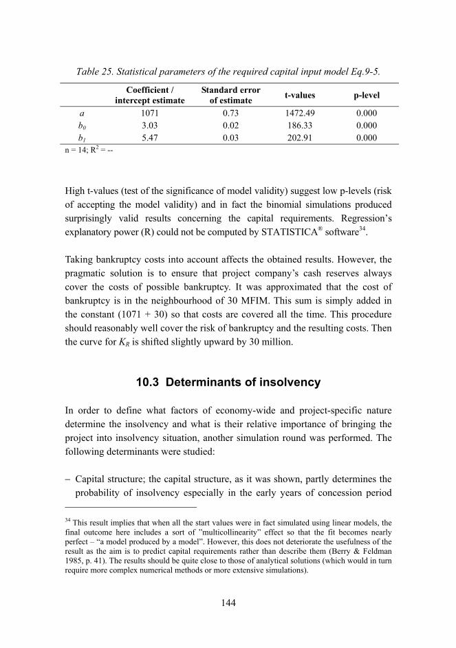
144

Table 25. Statistical parameters of the required capital input model Eq.9-5.

Coefficient / intercept estimate

Standard error of estimate t-values p-level

a 1071 0.73 1472.49 0.000 b0 3.03 0.02 186.33 0.000 b1 5.47 0.03 202.91 0.000

n = 14; R2 = --

High t-values (test of the significance of model validity) suggest low p-levels (risk of accepting the model validity) and in fact the binomial simulations produced surprisingly valid results concerning the capital requirements. Regression�s explanatory power (R) could not be computed by STATISTICA® software34.

Taking bankruptcy costs into account affects the obtained results. However, the pragmatic solution is to ensure that project company�s cash reserves always cover the costs of possible bankruptcy. It was approximated that the cost of bankruptcy is in the neighbourhood of 30 MFIM. This sum is simply added in the constant (1071 + 30) so that costs are covered all the time. This procedure should reasonably well cover the risk of bankruptcy and the resulting costs. Then the curve for KR is shifted slightly upward by 30 million.

10.3 Determinants of insolvency

In order to define what factors of economy-wide and project-specific nature determine the insolvency and what is their relative importance of bringing the project into insolvency situation, another simulation round was performed. The following determinants were studied:

− Capital structure; the capital structure, as it was shown, partly determines the probability of insolvency especially in the early years of concession period

34 This result implies that when all the start values were in fact simulated using linear models, the final outcome here includes a sort of �multicollinearity� effect so that the fit becomes nearly perfect � �a model produced by a model�. However, this does not deteriorate the usefulness of the result as the aim is to predict capital requirements rather than describe them (Berry & Feldman 1985, p. 41). The results should be quite close to those of analytical solutions (which would in turn require more complex numerical methods or more extensive simulations).

145

when capital reserves must cover all the cash outflows of the project company; amortisation and interest payments take a large share of the cash outflows and they increase in pace with leverage.

− Interest rate paid on debt; if interest rates get high the interest payments may increase to the amount where capital reserves are exhausted.

− Inflation; if inflation gets high, the construction and operating costs may increase by an amount that will be critical for the solvency.

− Traffic volumes; as traffic volumes dictate the cash inflows, it is obvious to study this factor�s influence on solvency.

Since all the prospective determinants of insolvency are not independent from each other their correlations with each other has to be analysed as well and then determine to what extent each determinant determines the insolvency. Another problem rises with the fact that insolvency is an accumulative process. The reason behind insolvency may lie in the previous years with exceptionally high expenses or low revenues. Therefore, just studying the actual year of insolvency occurring is not enough but one needs also to analyse the preceding years whether they include the seeds to the process leading to insolvency. Also the �exceptionality� of the parameter in question is one aspect that has an impact on exceptional results. Therefore the deviations and the magnitude of deviations from the expected values are of importance. The following model was tested:

+∆×+∆×+∆×+×+= CbcbHrbCapbaK

y 473721'

ε+∆×+∆× pVKTbOpeb 7675 (Eq.9-6)

where

yK� = remaining capital reserve after seven (2003) years from the starting of the concession period; this remaining reserve may be positive even if the insolvency has occurred in the previous years; however, it should be relatively small compared to those cases where insolvency did not take place

a = intercept term

bn = coefficients, n = 1, 2, 3, 4, 5, 6

146

Cap = capital structure, i.e. D/K -ratio in percentages

∆7rH = market interest rate for debt, annualized difference in percentage units from the annualized expected value for the seven first years (1997�2003) of the concession period

∆7c = inflation, annualized difference in percentage units from the annualized expected value for the first seven years of the concession

∆7C = percentage difference of the total construction cost from the expected value

∆7Ope = difference of operating costs from the expected values, first seven years, annualized percentage

∆7VKTp = traffic volume growth for the project, annualized difference in percentage units from the annualized expected value for the first seven years of the concession period.

The first seven years were selected as the critical period when the insolvency is most likely to take place, especially years 3...6 are critical when the capital reserves are consumed by the construction costs and debt service payments but revenues are still modest. If we keep the probability of success (i.e. no insolvency) of the project company at 90% level, we can use the capital requirement model (Eq.9-4) to determine the capital to be invested at each level of debt finance.

The following simulation procedure is used:

1. The capital structure starts from all-equity financed project company (D/K = 0 or 0%) and ends with D/K ratio of 0.57 (57%). In each simulation run set, the ratio is increased by 0.05 units (or 5% units respectively), except for the last round where the D/K ratio is increased only by 2% units, i.e. from 0.55 to 0.57.

2. At each step the simulation runs are repeated until two insolvency cases have occurred. Thus, there will be 26 insolvency cases altogether.

3. All other variables are simulated according to full project model that include predefined randomness for sub-models� variables.

147

4. The results, i.e. the insolvency cases, are then analysed with multiple regression method in attempt to explain to which extent each selected variable contribute to insolvency occurred.

5. The capital requirement model (Eq.9-4) is used to determine the capital input of equity and debt at each leverage level. The last capital structure ratio does not quite insure 90% success probability for the project company but still it is possible to use it to study what variables determine insolvency.

Otherwise the simulation process was as explained in Chapter 8.3. The results of simulation runs are listed in Table 26.

Table 26. Determinants of insolvency � results of 26 simulated insolvency cases.

Capital reserve in 7th year*

D/K ratio

Interest on debt,

annualized difference

Construction cost estimate

error

Operating costs,


Inflation, annualized difference

Project VKT,


yK� Cap ∆7 rH ∆7 C ∆7 Ope ∆7 c ∆7 VKTp 248.28 0 1.39 4.34 5.84 3.91 -0.39 281.71 0 0.52 2.55 3.78 1.52 -0.27 81.99 0.05 1.38 -5.30 4.55 6.01 -0.07 225.03 0.05 -3.18 -1.43 -1.72 3.29 -0.29 141.74 0.10 0.63 -1.07 1.75 4.05 0.64 140.03 0.10 -0.03 2.86 -5.41 4.21 -0.06 234.53 0.15 -1.96 6.42 -6.18 0.84 0.92 -33.05 0.15 2.74 -2.71 2.85 8.13 0.60 124.97 0.20 0.21 -1.62 4.81 2.53 -0.36 61.49 0.20 3.17 8.85 -5.35 3.55 0.01 157.44 0.25 1.63 3.29 0.81 -0.97 0.34 161.22 0.25 -0.96 4.53 4.25 2.29 0.59 41.05 0.30 0.17 1.18 -3.03 5.77 -0.22 78.99 0.30 4.11 1.08 -3.77 5.15 0.28 46.51 0.35 2.71 2.91 -1.05 3.85 0.64 33.11 0.35 1.20 0.44 6.12 4.11 1.56 29.79 0.40 0.58 -0.45 4.01 2.35 -0.20 80.07 0.40 1.33 0.37 0.38 4.31 0.19

-133.85 0.45 -1.46 1.74 9.89 0.69 -0.52 -24.29 0.45 4.75 -5.85 -4.87 1.98 0.85 -53.66 0.50 4.54 3.66 -10.43 -1.09 0.53 -166.92 0.50 -0.35 -3.97 -3.69 3.37 -0.99 -646.23 0.55 3.40 0.31 3.82 7.15 -0.10 -118.66 0.55 -0.90 2.38 1.80 6.58 0.53 20.84 0.57 0.52 6.78 -8.74 3.44 -0.62 -36.77 0.57 0.70 2.83 -0.58 7.59 1.16

* Even if capital reserve is positive in t = 7, the reserve has gone below zero at some point of time t = 1, 2, �7.

148

The results of multiple regression analysis are summarized in Table 27.

Table 27. Multiple regression results for Eq.9-7.


Standard error of estimate t-values p-level

a 317.3 55.71 5.695 0.000 b1 -680.6 126.3 -5.387 0.000 b2 -22.02 12.57 -1.752 0.100 b3 3.640 6.898 0.528 0.604 b4 -7.216 4.998 -1.444 0.165 b5 -19.55 9.982 -1.958 0.065 b6 65.04 39.47 1.648 0.116

n = 26; R2 = 0.707; F(6,19) = 7.643 > F.01(6, 19) = 3.94

Standardized regression coefficients show that capital structure has the most effect on poor cash reserve. Negative sign indicates that the more there is leverage, the poorer the cash reserve will probably be. Then comes the exceptional inflation rates (the more inflation above the expected rate, the poorer cash reserve), exceptional interest rates (the higher rate than expected, the poorer cash situation), and the traffic volume (the higher project VKT, the better cash position). Construction cost estimate error is a poor contributor to the regression equation and in fact the sign is in the wrong direction. As visible, all the regression coefficients except ∆C are quite surely different from zero, which is the null hypothesis tested and the t-values and resulting p-levels indicate the risk of making type I error, i.e. risk of rejecting null hypothesis when it would have been true (in this case, if the coefficient would have truly been zero). Especially the intercept term a and capital structure Cap are significantly different from zero at 99.99% confidence level (i.e. less than 0.1% risk or p-level). The other variables also perform well, in the neighbourhood of 90% confidence level. The overall explanatory power is quite good, too, and the whole equation is significantly at less than 0.1% p-level.

Since construction cost estimate error, or construction cost engineering error, is a insignificant contributor for the regression, a stepwise regression was carried out in the attempt to include only the contributing variables to the regression

149

equation. The results of stepwise regression are respectively as shown in Tables 28 and 29.

Table 28. Stepwise regression summary for Eq.9-7.

Variable included Coefficient


Standard error of estimate

t-values p-level

a 326.6 51.87 6.297 0.000 Cap b1 -680.0 124.0 -5.482 0.000 ∆7c b3 -20.63 9.590 -2.151 0.044

∆7Ope b5 -7.956 4.710 -1.689 0.107

∆7rH b2 -23.21 12.14 -1.913 0.070

∆7VKTp b6 67.51 38.48 1.755 0.095

n = 26; R2 = 0.703; F(5,20) = 9.457 > F.01(5, 20) = 4.10

A variable was entered to the regression equation when the test statistic F was greater than 1.00 (tested at 95% confidence level). F statistic�s square root is equal to t-test statistic, i.e. F1/2 = t, and thus are directly comparable with each other, resulting in same p-values (Hair et al. 1998, p. 200). The results without the cost estimate error ∆C are almost exactly the same as previously with regard to explanatory power of regression and statistical significance of coefficients and overall regression. The stepwise results are shown in Table 29. Correlations between all the variables in the original regression equation are shown in Table 30.

Table 29. Stepwise regression summary � variables� contribution to regression.

Variable entered

Coefficient / constant

Multiple (cumulative) R2

F to enter if > 1 p-level Tolerance

Cap b1 0.501 24.10 0.000 0.915 ∆7c b3 0.595 5.310 0.032 0.938

∆7VKTp b6 0.623 1.690 0.208 0.927

∆7rH b2 0.660 2.276 0.147 0.852

∆7Ope b5 0.703 2.854 0.107 0.871

150

Table 30. Variables� correlation matrix (Eq.9-7).

Variables Cap ∆7 rH ∆7 C ∆7 Ope ∆7 c ∆7 VKTp yK�

Cap 1.00 0.22 0.02 -0.21 0.08 0.09 -0.71 ∆7rH 1.00 -0.10 -0.25 0.08 0.25 -0.32 ∆7C 1.00 -0.28 -0.25 0.06 0.21 ∆7Ope 1.00 0.17 -0.04 -0.06 ∆7c 1.00 0.11 -0.36 ∆7VKTp 1.00 0.07 yK� 1.00

There is little risk for multi-collinearity between the variables as implied by the high tolerance values (Table 29). Usually the multicollienarity is considered non-distorting if the tolerance values are over 0.10 and correlations between independent variables in the regression are low (Hair et al. 1998, p. 193). This is the case with the obtained regression results, so the conclusion is that multicollinearity is not distorting the results.

The practical implications can now be interpreted and demonstrated. The clear implication is that once capital structure closes to 50% debt ratio, the risk for insolvency rapidly increases and more liquidity �buffer� is needed to keep the project company solvent. This was also observed in the capital requirements needed to ensure 90% solvency probability, as the capital requirement curve (Eq.9-5) went up after 40% debt ratio. Even if the other variables in the equation are zero (i.e. expected values) or close to zero the risk of insolvency is still great. We can say that the capital structure and the cash outflows resulted by amortisation and interest due to capital structure payments largely dictate the risk of insolvency. All other variables are then contributing to the risk: i) higher than expected inflation, affecting maintenance and construction costs; ii) higher than expected interest rate on debt contracts, affecting interest payments only; iii) operating costs different from expected; iv) and finally lower than expected traffic volume growth. Contribution to insolvency risk is not differing very much between the variables. These factors form the relevant risk profile for insolvency of the project company.

151

Even if multicollinearity does not have an effect on the results, the variables are of course somewhat overlapping with each other. Capital structure and interest rate are affecting the same cash flows, the debt service payments. Inflation and operating costs are also partly overlapping factors. However, in the latter overlapping case the difference from expected operating costs was computed on a nominal basis and thus it represents the cost estimating error for operating costs and its impact on insolvency. Inflation in turn may cause higher cash outflows even if the nominal cost estimating would have been accurate. Also inflation is affecting cash outflows of construction. In the case of capital structure and interest rate, the former is quite naturally the dominant factor because it includes two cash flow items, amortisation and interest payments. However, higher than expected interest rates clearly brings an additional effect.

10.4 Project�s cost of capital

10.4.1 Introduction � finding the correct discounting rates for valuations

Project cost of capital is needed for discounted cash flow analysis. Until here, nominal analysis was applicable, but valuation of the project as well as debt and equity require that a sound discounting rate is applied. Also valuation of the project and its capital components requires that the denominator in the valuation formula is fixed when applying a single-period valuation model. Denominator being fixed, we can analyse the numerators� contributions to project value and investors� wealth. Also the analysis of optimal capital structure requires that we fix the denominators in valuation formula.

10.4.2 CAPM-based cost of capital using un-relaxed empirical data

The project cost of capital is dependent on capital structure. The cost of capital determination can be found e.g. in Copeland and Weston (1988, pp. 456�469). Using Eq.4-18a and Eq.4-18b, the after-tax cost of risky debt is

( ) ( ) ( ) ⎥⎦⎤

⎢⎣⎡ −−+−=

DVdrrTk fEfcD 1N1 ρ

152

and the cost of equity is

( )( )EDTkk cDEEE −−+= 1ρρ

where

N(-d1) is the cumulative normal probability at point -d1 from N(0,1), and as in Eq.4-19,

tt

trDV

df

σσ 2

1ln1 +

+⎟⎠⎞

⎜⎝⎛

=

and V is the value of the project company, D is the value of debt of the project company, rf is the risk-free interest rate, t is the time to maturity of the asset and σ is the variance of the return on the asset. For debt and equity the book values have to be used as estimates. For risk-free interest rate the most likely estimate based on historical average for 1985�1995 risk-free rate was 10.8% (Nordiska Ministerrådet 1996). The historical average market return for 1981�1995 was 18.7% (Statistics Finland 1996; 1993; 1990)35. The maturity of the asset is the length of the concession contract, i.e. 15.33 years and the standard deviation of asset return is σ = (0.000133)1/2 = 0.01153. Unlevered equity�s beta βpU = -0.021 and thus it follows that ρE = 10.8 + (18.7-10.8)*-0.021 = 10.6. The calculation of beta is shown in detail in Appendix D as well as references to earlier beta estimate studies.

The weighed average cost of capital for the project is then, as implied by Eq.4-17c,

VEk

VDkrWACC EDp +==

35 A chained index had to be constructed for this, based on HEX-index issued by Helsinki Stock Exchange starting from year 1987 and on Unitas index, issued by Union Bank of Finland. The issuing of the latter index was ceased in 1990.

153

Hsia (1981) has showed that the result is finally36, as in Eq.4-18c,

⎟⎠⎞

⎜⎝⎛ −=

VDTWACC c1ρ

Hsia assumed that bankruptcy costs to the third parties besides shareholders and creditors are zero. This leads to WACC which varies according to the capital structure of the project company as illustrated in Figure 27. Table 31 shows the computed figures.

Table 31. Computed values for cost of capital.

D/V -d1 N(-d1) kD kE rp = WACC

0 -189.2 0 7.75 10.59 10.59 0.05 -102.7 0 7.75 10.70 10.44 0.1 -87.42 0 7.75 10.82 10.30 0.2 -72.09 0 7.75 11.11 10.00 0.3 -63.13 0 7.75 11.47 9.70 0.4 -56.76 0 7.75 11.96 9.41 0.5 -51.83 0 7.75 12.64 9.11 0.6 -47.80 0 7.75 13.67 8.81 0.7 -44.39 0 7.75 15.37 8.52 0.8 -41.44 0 7.75 18.79 8.22 0.9 -38.83 0 7.75 29.04 7.92

0.95 -37.64 0 7.75 49.53 7.77 1 -36.50 0 7.75 indefinite 7.63*

* This value correctly equals (1-Tc)ρE

Because the maturity of the asset is so long (15.33 years) and the variance of return on it low (standard deviation 0.01153), the �call option� of the project company�s equity is a �sure bet� so that the probability of loosing the invested equity (e.g. in case of bankruptcy) is zero. This conclusion is implied by the high

36 Hsia proved that the option theory and CAPM as well as Miller-Modigliani theorem are consistent.

154

values of -d1 which indicate long distance from the mean of distribution N(0,1), and thus N(-d1) is zero in all cases.

Figure 27. Cost of capital of the project company.

The above conclusion is in contradiction with the previous results concerning risk of insolvency. The risk of insolvency is quickly rising in pace with capital structure (other factors also contributing to insolvency, too) and if the investors are risk averse so that they want to ensure e.g. 90% success probability for the project company without insolvency situations, the investment is far from being low risk. The contradiction is explicable, however. The risk does not lie in the ultimate outcome of the project. The project will most likely be profitable for investors if the whole investment period is looked at. The risk lies in the cash flow profile of the project. If insolvency is not allowed in any way for the project company, the capital requirements increase and the probability of facing insolvency rise with leverage so that with more than 50% debt financing ratio the 90%-probability-no-insolvency requirement is impossible to reach in practice. If, and as surely is the case in practice, insolvency can be allowed by

Cost of equity

WACCρE

0.72 ρE

Cost of debt

Cos

t of c

apita

l (%

) 30

20

10

0 0 0,1 0,3 0,5 0,7 0,9 1

D/V ratio

155

employing some contracts or instruments that protect the company in insolvency situations in the first half of the concession period, the investors will with high probability get a positive return on their investment at the very end of the concession period. Simple instruments or contracts, such as generous overdraft limits or overdraft agreements combined with suitable bonds and guarantees provide likely solutions to the problem.

The 90%-probability-no-insolvency requirement, if applied, will have implications to the cost of capital, however. If overdraft agreements prove to be difficult to arrange and if the exhaustion of cash reserves proves to be truly risky leading possibly to bankruptcy, the required return on equity must rise steeper as the leverage increases. The threshold leverage ratio was 0.57 for the project company after which there was no guarantee that the project company will have 90% certainty of not encountering insolvency at any point of concession period. Thus, the real world cost of capital curve reaches value “indefinite” sooner than theory would suggest. But this depends only on the risk averseness of the equity investors and terms negotiated with other investors. This leads to the conclusion that each project carries unique profile for risk and cost of capital despite the fact that projects like the case project have probably very similar covariances with the market. CAPM has a statistical approach to risk and valuation of assets but clearly lacks more refined quantities to handle contingent investment situations. In other words, CAPM offers a rational tool for investment evaluation but does not take into account the obvious managerial/human pursue for safe decisions, i.e. safe investments. Very few, if anybody, will make serious, significant long-term investments with fifty-fifty chance of succeeding, which is the result when investment decisions are based on expected values. If investments made are large in numbers, as it is with professional stock trading, then the rationale of CAPM is acceptable and the end result will be positive for the skilful investor. Without this dispersion of risk enabled by many simultaneous investments, the risk for a single investment becomes significant and investors will seek for safer positions, ensuring high probability of success.

156

10.4.3 Cost of capital, relaxed estimates

10.4.3.1 Reference interest rates, relaxed estimates

For risk-free rate rf the empirical reference based on 1980�1996 data was 10.8%. In the light of more recent observations this seems high. For example, in 2001 the State of Finland issued a government bond for 11 years with nominal rate of 5.75% (Bank of Finland, www.suomenpankki.fi). During 1996�2000 the yields on Finnish benchmark government bonds varied between 7.08%...4.74%. Therefore, we can choose rf = 5%.

The market rates� recent intervals (for 1998�2004, 12 month Helibor) varied between 2.0%...5.3% (Bank of Finland, www.suomenpankki.fi), which is considerably lower than our time series estimates. However, the fluctuations in the long run may be considerable. Private placements bonds (i.e. smaller entity long term bonds) for 6 years paid typically 7%...8% nominal rate (Bank of Finland, www.suomenpankki.fi). The average lending rate of Finnish commercial banks to Finnish companies for 1990�2002 has varied between 15%...3%. In 1996 and 1997 the average lending rate was between 4%...6% (see e.g. Koskenkylä 2002, p. 140). If our case project�s debt maturity would be 15 years, we could assume slightly higher nominal rate because of term structure of interest rates. We assume 6% including the premium for risk.

For market return we have a historical annual average E(rm) = 18.7% for 1981�1995 using chained market indexes (Leviäkangas 1998). This estimate is very high. HEX all-share index for 1999�2004 varied roughly between 5000 and 18000 points the highest peak reached in year 2000 and lowest 2003. The annual returns varied roughly between 130%...-40% (HEX Integrated Markets Ltd., www.hexgroup.com). It is evident that even longer time series cannot be very reliable. Therefore, we can start from the earlier estimate of expected annual return for diversified market investment (E(rm) = 18%) but keeping in mind that markets have changed to more efficient which will lower the returns from the market. We assume E(rm) = 12%.

157

10.4.3.2 Cost of equity

The cost of equity estimate in a normal CAPM framework is determined by (see e.g. Copeland & Weston 1988, p. 456)

kE = rf + { E(rm) � rf }βpL = 5% + (12% � 5%)βpL (Eq.9-8)

and yields to cost of equity rates as shown in Table 32. The risk premium for Finnish listed equity markets have been, for example, about 4 percent units in 1997 (Kallunki et al. 2001, p. 113). Our calculation is 7 percent units, which is within reasonable limits taking into account that a) the project company is not publicly listed and b) similar investments are not quoted by the market.

Table 32. Relaxed estimates for cost of equity.

Leverage, D/V Levered beta, βpL Cost of equity, kE

0 0.2 6.40% 0.1 0.22 6.51% 0.2 0.24 6.65% 0.3 0.26 6.83% 0.4 0.3 7.07% 0.5 0.34 7.41% 0.6 0.42 7.91% 0.8 0.78 10.43% 0.9 1.5 15.47%

The cost of equity is low, as it should be when the beta is as low as 0.2. This result does not take into account the high risk of insolvency and further, the risk of bankruptcy, but does significantly contribute to the risk profile of case project. In reality, we can assume higher increase of cost of equity as a function of capital structure.

10.4.3.3 Cost of debt

The simulated forecast for cost of debt (rH) suggested very high debt contract interest rates, i.e. between 13%�14%. This was regarded too high in the light of more recent data and alternative estimates were driven with other methods.

158

Damodaran gives the following alternative paths for cost of debt estimation in the case of non-traded private firms (Damodaran 2005a, p. 12):

− borrowing rate of recent raising of debt by the firm − average cost of debt for the industry, in which the firm can be categorized − estimating synthetic rating for the firm and using corresponding cost of debt.

Here we follow the third path. Damodaran (2005b) uses the categorisation following Table 33 for smaller and riskier companies to estimate the rating and spread (additional risk premium) on the basis of long-term interest coverage (net earnings before interest and taxes divided by total interest payments).

Table 33. Synthetic rating and spreads for smaller and riskier firms.

Interest rate coverage threshold: Rating Spread

< 0.50 D 14.00% < 0.80 C 12.70% < 1.25 CC 11.50% < 1.50 CCC 10.00% < 2.00 B- 8.00% < 2.50 B 6.50% < 3.00 B+ 4.75% < 3.50 BB 3.50% < 4.50 BBB 2.25% < 6.00 A- 2.00% < 7.50 A 1.80% < 9.50 A+ 1.50% < 12.5 AA 1.00% >12.5 AAA 0.75%

For the project company, the interest coverage is changing as the project matures. The early stages are risky as analyses of insolvency explicitly demonstrated and the interest rate coverage is low. As the project matures the interest coverage improves and thus the rating should also change in pace of project�s life. But it is obvious that debt capital suppliers look at the riskiest phases of the project and assess their risk premiums according to those foreseeable risks.

159

If we assume that the first seven years of the concession contract represents the high risk part of the project and calculate the cumulative interest coverage in nominal terms (cumulative revenues divided by cumulative interest payments) and at the same time using the expected values for traffic growth, construction and operating costs, the obtained interest coverage for different capital structures of the project company are as shown in Table 34. Two alternatives for capital input has been used, the KR coming from insolvency analysis and fixed capital input of 1 billion FIM (Kfixed).

The table shows that

− whichever capital requirement criteria is used, the interest coverage ratios are not very much differing; both methods are thus available when assessing cost of debt risk premiums; however, KR definition does not allow debt capital to rise over debt capacity 57%

− the cost of debt is highly dependent on terms of concession contract and in this case, especially on the agreed unit toll to be received by project company; this provision naturally requires that debt financiers have all the relevant information on project risks at their disposal.

Table 34. Interest coverage; cash flow before interest and taxes divided by interest.

If unit toll = 0.5 FIM If unit toll = 0.9 FIM D/V If Kfixed

= 1000 mill. FIM If using KR If Kfixed 1000 mill. FIM If using KR

0 - - - - 0.1 1.74 1.57 10.1 9.09 0.2 0.87 0.77 5.03 4.44 0.3 0.58 0.49 3.35 2.85 0.4 0.43 0.35 2.52 2.00 0.5 0.35 0.25 2.01 1.45 0.6 0.29 Not financed 1.68 Not financed 0.7 0.25 Not financed 1.44 Not financed 0.8 0.22 Not financed 1.26 Not financed 0.9 0.19 Not financed 1.12 Not financed 1 0.17 Not financed 1.01 Not financed

160

Using Damodaran�s synthetic rating tables and assuming KR the cost of debt can be approximated according to Table 35. The result is interesting, for it suggests that cost of debt ranges from roughly 7% (6.75% exactly; 6%+0.75%) to 20% (6%+14% = 20%) and thus exceed the cost of equity estimates. However, the results are intuitively to the right direction if we recall the implications from insolvency analysis.

If we relax the debt capacity assumption and use Kfixed we obtain the following after-tax cost of capital figures for different revenue projections depending on selected unit toll (Table 36).

Table 35. Synthetic estimates of premiums on cost of debt.

Spread on cost of debt capital, % units D/V Unit toll

= 0.3 Unit toll

= 0.5 Unit toll

= 0.7 Unit toll

= 0.9 Unit toll

= 1.1 0 - - - - -

0.1 8.00% 2.00% 1.00% 0.75% 0.2 12.7% 4.75% 2.25% 1.80% 0.3 14.0% 8.00% 4.75% 2.25% 0.4 14.0% 11.5% 8.00% 4.75% 0.5

coverage negative, spread at

least 14%-units in all

cases 14.0% 11.5% 10.0% 6.50% > 0.57 Not

financed Not

financed Not

financed Not

financed Not

financed

161

Table 36. After-tax cost of capital estimates; debt capacity assumption relaxed.

after-tax kD = (1 � Tc)(6% + spread); Tc = 0.28 D/V kE Unit toll

= 0.3 Unit toll

= 0.5 Unit toll

= 0.7 Unit toll

= 0.9 Unit toll

= 1.1 0 6.40% 4.32% 4.32% 4.32% 4.32% 4.32%

0.1 6.51% 14.4% 10.1% 5.76% 5.04% 4.86% 0.2 6.65% 14.4% 12.6% 7.74% 5.76% 5.62% 0.3 6.83% 14.4% 13.5% 10.1% 6.84% 5.76% 0.4 7.07% 14.4% 14.4% 11.5% 7.74% 5.94% 0.5 7.41% 14.4% 14.4% 12.6% 9.00% 7.74% 0.6 7.91% 14.4% 14.4% 12.6% 10.1% 9.00% 0.7 8.85% 14.4% 14.4% 12.6% 11.5% 9.00% 0.8 10.4% 14.4% 14.4% 13.5% 11.5% 10.1% 0.9 10.5% 14.4% 14.4% 13.5% 12.6% 10.1% 1 14.4% 14.4% 13.5% 12.6% 11.5%

When reviewing the above cost of capital estimates it is evident that already this analysis shows that the project is viable with fairly high unit tolls and the highest tolls result in the soundest estimates for kE and kD. The same observation is confirmed when calculating the net present value of the project. The standard approach using interest coverage in order to determine the risk premium is weak in recognizing the insolvency risk as leverage increases. In other words, it would make more logic, if the cost of equity rose more sharply as leverage increases.

10.4.4 Discussion

The cost of capital estimates were derived using two methods. The first was based on risk-return theory and option theory and can be regarded as fundamentalist approach. The second method was based on the use of standard CAPM and synthetic rating of the project company. This could be regarded as standard approach. The two methods are characterized as follows:

162

Fundamentalist

− empirical averages of market variables (market return, risk-free rate, lending rate)

− estimates of unlevered beta, allowing negative beta

− combining CAPM and option theory

− taking into account the maturity of the asset, i.e. the length of concession contract.

Standard

− relaxed estimates of market variables, based on more recent market data − relaxed estimate of unlevered beta − synthetic rating of the project company.

The results are summarized in Table 37.

Table 37. Summarising the results of cost of capital estimations (after-tax cost of debt).

Fundamentalist approach Standard approach (Unit toll = 0.7 FIM) D/V

kE kD kE kD 0 10.59% 7.75% 6.40% 4.32%

0.1 10.82% 7.75% 6.51% 5.76% 0.2 11.11% 7.75% 6.65% 7.74% 0.3 11.47% 7.75% 6.83% 10.08% 0.4 11.96% 7.75% 7.07% 12.60% 0.5 12.64% 7.75% 7.41% 12.60%

> 0.57 Not financed Not financed Not financed Not financed

Fundamentalist approach is insensitive to revenues and relies solely on unlevered beta of the project and the market variables (risk-free rate, market return) but for the reasons discussed in 8.51 does not provide good estimates for

163

cost of debt which should change according to leverage of the project company. The estimates for cost of equity are more logical but very modest taking into account the risk of insolvency. Standard approach based on unlevered and levered betas and synthetic ratings of the project company provides logical estimates for cost of debt, but cost of equity estimates, not recognising the high insolvency risks, are inconsistent with cost of debt estimates. Cost of equity estimates do not rise as sharply with leverage as one would expect.

In order to be able to produce sound indications about optimal capital structure of the project company we need to obtain reasonable estimates for cost of capital. Neither of the approaches provides the solution. The fundamentalist approach seems to capture best the estimates of cost of debt. Standard approach suggests that the cost of equity should roughly exceed at 50% the after-tax cost of debt when leverage is low and when leverage increases the estimates become more biased. Fundamentalist approach suggests that cost of equity exceeds after-tax cost of debt roughly 40% in case of low leverage. Therefore, new estimates for cost of capital are produced based on synthetic rating and after-tax cost of debt pending on it. This yields to reasonable cost of debt estimates that take into account leverage and cost of equity estimates that likewise follow leverage and stay on the right level when leverage increases.

If we assume that kD is as estimated by standard method and kE is always 50% higher, i.e. kE = 1.5×kD and after these strong assumptions we also round the figures and re-estimate the cost of debt for higher leverage, we obtain the results of Table 38.

Table 38. Estimates of cost of capital for the case project.

D/V kE kD (after-tax) WACC

0 6% 4% 6% 0.1 9% 6% 8.7% 0.2 12% 8% 11.2% 0.3 15% 10% 13.5% 0.4 19.5% 13% 16.9% 0.5 24% 16% 20%

> 0.57 not financed

164

For practical calculations we assume these estimates, which reflect higher return demands on the basis of the following arguments: 1) the company is a pioneering enterprise in Finland37; 2) the project company is non-listed; 3) the complete risk profile is not well known by investors and even the non-significant risks are included; 4) double-counting of risks probably occurs because risk relationships are not known or not admitted in order to reach a better negotiation position; 5) finally, it is assumed that the high risk of insolvency is recognized.

10.5 Optimal capital structure

Optimal capital structure of a firm has been studied widely and corporate finance textbooks almost without exception deal with the issue. For papers about capital structure from different viewpoints, see e.g. DeAngelo and Masulis (1980), Dias and Ioannou (1995), Hong and Rappaport (1978), Kim (1978), Shah and Thakor (1987). Dias and Ioannou focused specifically on project company issue.

Fundamentalist approach suggested as much debt financing as possible whereas insolvency analysis suggested that the maximum debt ratio is 57%. This ratio also maximizes tax benefits of the project company. Standard cost of capital estimates suggest that WACC is in its minimum when debt ratio is 0% (or close to it) and thus the results are very much controversial. Optimal capital structure in standard approach is dependent on revenue projections which have an affect on interest coverage which in turn result in synthetic rating for the project.

The weighed average cost of capital for different unit tolls (which are building revenues which affect interest coverage) are as shown in Table 39. The minimum WACC that exceeds zero debt starts to appear after unit toll reaches 0.9 FIM. As the rating improves and cost of debt declines the more benefits are to be gained from debt financing � optimal capital structure moves towards higher leverage.

37 The investors of the project company represented a group that had quite substantial experience in BOT projects. Thus, the project company arrangement was a novelty only in Finland, but for investors the project represented a routine object.

165

Table 39. WACC for different unit tolls and capital structures.

WACC D/V Unit toll

= 0.3 Unit toll

= 0.5 Unit toll

= 0.7 Unit toll

= 0.9 Unit toll

= 1.1 0 6.40% 6.40% 6.40% 6.40% 6.40%

0.1 7.30% 6.87% 6.44% 6.36% 6.35% 0.2 8.20% 7.84% 6.87% 6.47% 6.44% 0.3 9.10% 8.82% 7.81% 6.83% 6.51% 0.4 10.00% 10.00% 8.85% 7.34% 6.62% 0.5 10.91% 10.91% 10.01% 8.21% 7.58% 0.6 11.80% 11.80% 10.72% 9.21% 8.56% 0.7 12.74% 12.74% 11.48% 10.72% 8.96% 0.8 13.61% 13.61% 12.86% 11.30% 10.15% 0.9 14.51% 14.51% 13.66% 12.89% 10.62%

10.6 Value of the case single-project company

We assume 1000 FIM total capital input and use the expected values for traffic demand, construction expenses and operating costs. Further, we use the WACC estimates from Table 39 to estimate the market values of the project (Vp , Dm , Em), returns on capital (Rp , RD , RE) and net present value to project investors (NPV_PI). These estimates are now based on average values of the full project model.

NPV_PI estimates are shown in Figure 28, showing the results for different unit tolls.

166

Figure 28. NPV_PI in the case of different unit tolls.

The estimates show that if the project is to be fully financed with private capital, including construction, required return on equity (although equal to risk-free return) and preparing for re-financing needs, the required unit toll rises sharply. Unit toll of 0.7 FIM clearly produces critical threshold value for the case project. Lower unit toll values were not included in the estimation since they produce only negative NPV_PI and thus are unacceptable for any private investor. The practical implication is that the assumption of 0.3 unit toll made in the early stages of the project, is not nearly enough when all the project costs and working capital requirements are covered by the project company and its investors and the investors are expected to have a return on their investment.

The market value of the project for different unit tolls is shown in Figure 29.

2000

1500

1000

500

0

-500

-10000 0,1 0,2 0,3 0,4 0,5 0,6 0,7 0,8 0,9

Unit toll = 0,7 Unit toll = 0,9 Unit toll = 1,1

NP

V_P

I

167

Figure 29. Value of project (Vp).

The value of the project as well as NPV_PI are maximized when debt ratio is 10% as should be the case when WACC is minimized at this point. The exact points for minimum WACC and maximum values were not estimated. The market values of project, debt and equity are presented in Figures 30�33. It shows that even with 1000 FIM capital input the market value of equity crashes down after 50% debt financing. This result is in line with insolvency analysis which used lower unit toll value of 0.3 FIM. If Em reaches zero the equity investors have no motive to be involved in the project and the project may go bankrupt and the debtholders stop receiving debt payments. Then the debtholders are in position to take over and if the project continues to loose money their wealth, the value of Dm, starts diving as well.

2500

2000

1500

1000

500

0

0 0,1 0,2 0,3 0,4 0,5 0,6 0,7 0,8 0,9

Unit toll = 0,7 Unit toll = 0,9 Unit toll = 1,1

V p

168

Figure 30. The market values of project, debt and equity; unit toll = 0.7 FIM.


1200

1000

800

600

400

200

00 0,1 0,2 0,3 0,4 0,5 0,6 0,7 0,8 0,9

D/K

Mar

ket v

alue

s (U

nit t

oll =

0,7

)

Vp

Dm

Em

Mar

ket v

alue

s (U

nit t

oll =

0,9

)

2000

1500

1000

500

00 0,1 0,2 0,3 0,4 0,5 0,6 0,7 0,8 0,9

Vp

Dm

Em

D/K

169


The value maximising points are rising slowly as the unit toll increases. In the case of 1.1 FIM unit toll the equity investors still have a motive to stay with the project company although they may be loosing a part of there investment if debt levels are raised sharply. This is visible also from Figures 33, 34, and 35 showing the returns on capital.

Figure 33. Returns on project, equity and debt, unit toll = 0.7 FIM.

Mar

ket v

alue

s (U

nit t

oll =

1,1

)

2500

2000

1500

1000

500

0 0 0,1 0,2 0,3 0,4 0,5 0,6 0,7 0,8 0,9

Vp Dm Em

D/K

2

1,5

1

0,5

00 0,1 0,2 0,3 0,4 0,5 0,6 0,7 0,8 0,9

Rp RD RE

D/K

Ret

urns

on

capi

tal (

Uni

t tol

l = 0

,7)

170



Ret

urns

on

capi

tal (

Uni

t tol

l = 0

,9)

2

1,5

1

0,5

0

Rp

RD RE

0 0,1 0,2 0,3 0,4 0,5 0,6 0,7 0,8 0,9 D/K

Ret

urns

on

capi

tal (

Uni

t tol

l = 1

,1)

3,5

3

2,5

2

1,5

1

Rp RD RE

0 0,1 0,2 0,3 0,4 0,5 0,6 0,7 0,8 0,9

D/K

171

10.7 Determinants of market value

The WACC is set to 8.2% according to 50% debt ratio and 0.9 FIM unit toll. Corporate tax rate is assumed constant over time, Tc = 28%. Relaxation of these assumptions means that scenarios for some variables are predetermined whereas the rest of the parameters are allowed to fluctuate on the time scale. This is a necessary precondition to have the denominator constant and to see what numerators� (i.e. cash flow affecting parameters) impact on project value is likely to be.

We will investigate how the following parameters determine the NPV_PI of the project:

− Economic growth, GDP, and traffic volume on the road, VKTp; these parameters dictate largely the traffic growth in general and on the specific road section and thus determine the shadow toll revenues.

− Construction cost C that is the largest single cash flow item for the project company and furthermore, timed at the very beginning of the project; deviation from planned estimate, the cost estimating error of construction cost, is expected to affect NPV_PI.

− Inflation c, affecting operating costs, Ope, and construction cost C.

The reasons for the selection of these parameters are the following. First, we know that traffic volumes are to a large extent dictated by macro-economy. However, it is not known on which predicted or anticipated parameters the investors should focus their attention. Should they rely on macro-economic forecasts only? Or should they be more specific and first focus on macro variables, and then closer on project-specific factors? The former is much easier to do in practice whereas the latter analysis requires much more management effort. The result will be interesting from the viewpoint of project investment planning. Secondly, the cost engineering inaccuracies can play a significant part in the value building process since it is timed at the beginning of the project. How significant this impact can be in relation to other impacts? Third, inflation is the only significant external factor affecting cash outflows as found in insolvency analysis. Operating cost variations due to weather and other condition variations did not play a very significant role in insolvency

172

contribution and thus it is left aside because it had only minor impacts on cash flows of the project company.

The following model was tested:

ε+×+∆×+×+×+= AjjpAjAjj cbCbVKTbGDPbaPINPV 4321_ (Eq.9-9)

where

jNPV_PI = project investors� incremental, surplus, after repayment of their capital in simulated case number j

a = intercept term

bn = regression coefficients, n = 1, 2, ..., 5

jGDPA = annualized economic growth in percent units for the whole concession period; simulated case number j

jVKTpA = annualized project -specific traffic growth in percent units for the concession period; simulated case number j

j∆C = construction cost estimate difference in percent units from the planned expected cost estimate in simulated case number j

jcA = annualized inflation in percent units for the concession period in simulated case number j

j = simulated case number, j = 1, 2,�, 30

ε = error term.

30 rounds of simulations were run calculating each time the NPV_PI from the discounted cash flows and keeping the WACC constant. The results of simulations are shown in Table 40. The regression results are summarized in Tables 41 and 42.

173

Table 40. Simulations of NPV_PI.

Case no j jNPV_PI jGDPA jVKTpA j∆C jcA

1 441.83 2.11 3.51 -4.55 9.19 2 266.63 2.02 2.77 -6.59 6.82 3 338.50 2.07 3.07 -7.17 8.52 4 420.04 2.37 3.67 -0.01 6.08 5 437.97 2.35 3.76 1.01 7.65 6 285.38 2.46 3.28 3.88 6.27 7 296.43 1.19 3.16 5.01 2.27 8 403.01 2.31 3.27 2.08 10.4 9 404.52 2.32 3.34 1.07 6.98

10 320.32 2.45 3.22 -5.64 3.68 11 401.89 1.66 3.55 -5.56 5.62 12 411.32 2.27 3.47 -3.42 4.37 13 362.72 2.21 3.55 -2.66 4.20 14 316.30 1.40 3.21 -4.25 4.64 15 576.48 2.35 3.75 -0.42 6.89 16 341.74 2.24 3.62 4.91 3.72 17 455.06 2.29 3.76 -1.60 8.78 18 218.92 1.27 2.48 -0.31 4.12 19 315.70 2.26 3.28 0.91 2.60 20 325.61 2.12 2.84 -2.50 7.83 21 260.47 3.04 3.37 1.14 6.24 22 -46.76 -0.39 1.95 -7.58 -2.39 23 168.94 0.25 2.76 4.14 3.88 24 324.07 2.14 3.21 6.99 6.86 25 300.88 2.27 3.24 1.06 4.15 26 315.59 2.44 3.65 -0.53 8.18 27 514.94 0.72 3.45 3.52 2.87 28 309.15 1.49 3.11 5.28 3.72 29 407.97 1.31 2.59 -2.04 4.56 30 342.74 2.52 3.27 7.07 4.40

Table 41. Summary of stepwise regression for Eq.9-9 � variables� contribution.

Variable entered Coefficient Multiple

cumulative R2 F to enter if

> 1 p-level Tolerance

jVKTpA b2 0.589 40.1 0.000 0.543

jcA b4 0.630 3.05 0.093 0.590

jGDPA b1 0.647 1.20 0.283 0.428

j∆C b3 not entered

174

The most significant contributor to NPV_PI was project-specific traffic volume. This is the basis of revenue for the project company. The other significant factor was inflation affecting cash outflows and namely construction costs and operating costs. The results are interesting thinking of the questions set previously. Clearly the project investor risk lies in the traffic volume, and not that much on general economic growth. This makes project investment planning a more challenging task and the analysis framework seems to be contingent. Inflation contributes to investor risk in terms of value building, but its impact is surprisingly modest. Cost engineering error is not contributing to NPV_PI, i.e. project investors� wealth increase. However, Tables 41�43 show that multicollinearity may be a problem here. All the included variables are significantly (p < 0.05) correlated with each other and correlation coefficients are not too low. Tolerance values are not very high either, although still well exceed 0.1, the value that can be regarded a rule-of-thumb threshold. This means that individual variables� contribution to NPV_PI can be regarded somewhat reliable.

Table 42. Multiple regression results summary for Eq.9-9.

Variable included

Coefficient / intercept


Standard error of estimate

t-values p-level

a -323.7 112.2 -2.884 0.008 VKTpA b2 200.2 42.56 4.704 0.000 cA b4 13.56 6.577 2.061 0.049 GDPA b1 -29.78 27.19 -1.095 0.283

n = 30; R2 = 0.647; F(3, 26) = 15.87 > F.01(3, 26) = 4.76

Table 43. Variables� correlation matrix (Eq.9-9).

Variables GDPA VKTpA cA ∆C

GDPA 1.00 0.67 0.63 0.11 VKTpA 1.00 0.49 0.23 cA 1.00 -0.04 ∆C 1.00

175

Recalling the cash flow impacts of time delays (Chapter 6.3.3), the revenue loss per month was ranging from 7.5 million FIM to 22.4 million when the unit tolls ranged from 0.3 to 0.9 correspondingly. The impact of revenue loss on market value can be simply estimated as a percentage of the market value, because the early revenues that were lost have a direct impact on present value of cash inflows. With low leverage of 10% debt (which yields to maximum project company value) the impacts of one month delay on project values are approximately

for 0.7 FIM unit toll => 17.4 mill. FIM / 1077 mill. FIM = 1.6%

for 0.9 FIM unit toll => 22.4 mill. FIM / 1551 mill. FIM = 1.4%.

As the leverage increases the relative impact will increase. We can conclude that one month delay will decrease project value between 1%...2%. Hence, the delays of having the project in operation can be regarded a fairly significant determinant too. Vice versa, early opening will result in added project value.

10.8 The state�s economic positions

The state must compare two alternatives: 1) the state invests in constructing and maintaining the project; 2) the state concessions the project and pays shadow tolls for the project company. In both cases, it receives the socio-economic benefits generated by the project. Table 44 shows the rather simple comparison.

Table 44. The state�s economic positions in conventional investment and in shadow toll cases.

Conventional state investment Shadow toll project

Costs Construction -C Shadow toll payments -Rev Operating costs -Ope Benefits Socio-economic benefits +Ben Socio-economic benefits +Ben Tax revenues +Tax

176

In conventional case, the state will construct the project and maintain it. Both are done via competitive bidding. In shadow toll arrangement, the state concessions the project and pays service (shadow toll) payments to the project company. It also receives corporate taxes from the project company. There is a justified question whether corporate taxes of the project company should be at all included in this calculus, since also the contractors building and maintaining the road in conventional case would equally pay corporate tax and in the above these taxes are not taken into account. However, we will keep the corporate taxes paid by the project company included as the analysis proceeds.

Now, in order for the shadow toll arrangement to be more beneficial to the state than the conventional case the following condition must be met:

Rev � Tax ≤ C + Ope (Eq.9-10)

If Tax is left out, the condition will be harder to fulfil, so including it will clearly relax the condition.

If the state invests in and operates the road itself, it needs to take into account the financing expenses as well as the expenses of construction and operation. In 1995 the Finnish Ministry of Transport and Communication used 5% discounting rate (Ministry of Transport and Communications 1994) for physical infrastructure investments and we can assume that this rate represents all the risk-adjusted costs of capital for the state. The benefits produced by the new road are greater the sooner the road is in service for road users, and therefore the timing of the investment is affecting the state�s economic position. The benefit-cost ratio of the investment is likewise critical. The better the ratio the sooner the project should be invested in. In road projects, the benefits are almost directly a result of the traffic volume. In the case project, the benefit of high traffic demand is offset by higher shadow toll payments. In every agreed shadow toll road project, the state�s willingness to pay for available infrastructure is measured. �Willingness�, however, can be different from project to project and depend on multiple factors beyond the scope of this research.

If we assume that neither the state nor the private investors have possibilities for extraordinary gains when it comes to construction and operating costs, one issue for the state is the timing of the investment and whether it can gain by speeding

177

up highly beneficial investments. The state also assumes a longer investment horizon than private investors. Typical period for which the investments in physical transport infrastructure are analysed is 20 years, but since the benefits accrue similarly even after possible concession periods the comparative analysis should be done for the concession period only.

We assume that the state is willing to invest in the construction C = 570 MFIM and bear the expenses of operating (Ope) as long as the benefit cost ratio exceeds one and the benefits (Ben) include the standard socio-economic project evaluation items:

− time savings of travellers and freight transport − vehicle cost savings (less wear and tear, less fuel consumption) − accident cost savings − other externalities that are evaluated along the project, such as noise and

pollution.

The state is assumed to receive Ben on behalf of road users, who ultimately receive it. The project�s benefit cost ratio, as it would typically be appraised in conventional case, is written as

B/C = Ben / (C + Ope) (Eq.9-11)

The shadow toll arrangements require that the state looks at the socio-economic benefits (Ben) as well as the tax revenues (Tax) provided by the project company and the shadow toll it must pay (Rev). Construction and operating expenses are not part of state�s cash flows any more. Then the ratio

(Ben + Tax) / Rev = BS / CS (Eq.9-12)

shows the benefit cost ratio for the state in shadow toll arrangement.

Using the expected values for construction expenses, operating expenses and vehicle kilometres of travel, and further assuming a 1000 MFIM capital input and debt ratio of 20% (for corporate tax calculation, i.e. Tax) we can estimate

178

how BS /CS behaves when the projects benefit cost ratio changes, i.e. Ben varies38. The viewpoint is from the situation when the state considers different projects and how to implement them and compares different financing and operating options. Figure 36 shows how BS /CS behave under these assumptions with different unit tolls paid by the state and different initial project benefit cost ratios (B/C).

Figure 36. State�s total benefits and costs in shadow toll arrangement when project�s benefit cost ratio varies.

In the light of the case project, Figure 36 results in a straightforward conclusion: only projects with very high socio-economic benefit cost ratio produce net benefits for the state in shadow toll framework and even then this framework has to be combined with low shadow toll payments. The lowest unit toll of 0.3 FIM produces BS /CS ratios exceeding one. The second lowest analysed unit toll results in positive net outcome for the state if the project�s B/C exceeds two. This result clearly points out the problematic interest conflict between the state as ultimate customer for the project and project investors seeking return on their investment.

38 1000 MFIM input is regarded here as reasonably close to 1065 minimum capital requirement and 20% debt ratio reasonably close to optimal capital structure which varied between 0%...10% depending on negotiated unit toll (see Chapter 9.6).

2

1,5

1

0,5

01 1,3 1,6 1,9 2,2 2,5

Project�s B/C

Unit toll = 0,3

Unit toll = 0,5

Unit toll = 0,7

Unit toll = 0,9

Unit toll = 1,1

Sta

te�s

tota

l ben

efits

/ to

tal c

osts

179

The previous analysis assumed constant debt ratio for the project. Holding all the other assumptions, but changing the capital structure and using the unit toll = 0.7 FIM we can assess how sensitive the BS /CS ratio is for different financing mixes of debt and equity (Figure 37). The capital structure affects the tax revenues received by the state: the higher the leverage the less the corporate taxes paid by the project company.

Figure 37. The sensitiveness of state�s economic position to project company capital structure.

Again, the conclusion is obvious: changes in the capital structure of the project company bear little meaning to the state. Changing any of the assumptions does not change this conclusion. Assuming different B/C ratios do not change the insensitiveness, though it may change other state�s decisions such as preferring high equity input as suggested by many studies. It seems that equity input as such should be rather irrelevant for the state from a purely financial and economic point of view. However, the psychological stature of equity commitment remains, although the economic relevance varies from case to case and depends on contractual structures between the state and project company or project company investors.

Sta

te�s

tota

l ben

efits

/ to

tal c

osts

0 0,2 0,4 0,6 0,8

1

0,8

0,6

0,4

0,2

0

D/K

B/C = 1

B/C = 1,3

B/C = 1,6

B/C = 1,9

B/C = 2,2

B/C = 2,5

181

PART V: SUMMARY OF RESULTS AND EVALUATION

In this section, the results are summarized. First, the investors� risks are ranked based on the full project model and simulation followed by risk mitigation strategies recommended to investors. The shadow toll arrangement is evaluated from multiple angles � what type of projects and what type of investors seem to be appropriate for shadow toll projects. Also some policy recommendations are provided. The evaluation is based on model and simulation results, but the results are reflected to some recorded experiences from similar financing arrangements and projects.

Methodological issues, mainly related to the application of CAPM are discussed after modeling and simulation results.

Recent empirical data on the case project is reviewed and reflected to model results. Main emphasis is on the project company information (financial statements) because that is available from public records. The concession contract terms remain confidential but on the other hand, the actual contract was not the focus of the research per se. The model seems to work and perform satisfactorily.

Finally, the overall results are summarized, concluded and visualized. All the research questions are answered one by one and the constructed model is evaluated as a whole. Also the overall methodological approach is being evaluated � how and in what conditions can the approach be applied. Further research needs are issued at the end.

183

11. Risk profile of the case project

11.1 Investor risks

We found out that the project company�s beta is close to zero, although in calculations we assumed 0.2 beta. Close-to-zero result is in accordance to previous published case project calculations (Leviäkangas 1998) and somewhat similar to those of Khan and Fiorino (1992) although their projects were very different in magnitude and scope. However, the common factor is the low volatility of cash flows which in the end dictate the beta estimates in non-publicly-quoted cases. Whatever the methods of beta estimations are the evident result is that risk-adjusted cost of capital in equity financed projects seems to draw near the risk-free rates, or possibly even be slightly counter-cyclical. Corporate finance theory identifies countercyclical betas, so this finding is nothing new. Low-risk and low-beta projects are interesting to those financiers who seek long-term, low-risk investments and have the capacity to allocate large amounts of capital at one time.

On the other hand, the risk of insolvency seems particularly high for the case project and the working capital requirements are substantial compared e.g. to estimated construction cost. The case project�s requirement of working capital when the investors try to ensure 90% success against insolvency in all situations during the concession increases the capital requirement to almost double that of construction cost. This will be reflected to cost of capital if investors are aware of this. The most critical factors resulting insolvency are

− the capital structure (the more debt, the higher risk for insolvency situations) − inflation yielding to higher construction and operating costs − higher than expected rates on debt contracts if fluctuating rates are employed − higher than expected operating costs, i.e. maintenance of the road − lower than expected traffic volume.

The debt capacity of the project company when assuming the lowest analysed unit toll of 0.3 FIM per vehicle kilometre of travel was found to be 57%. It is obvious that once the unit toll is increased the debt capacity is raised as well. However, it will not significantly change the optimal capital structure of the

184

project. The liquidity is improved and thus the risk of insolvency reduced in pace of higher tolls.

The market value of the case project is very much dependent on the negotiated unit toll. The first insights of reasonable unit toll were completely underestimated. This is probably because of number of reasons. First, the total risk profile and different risk elements were not fully known by negotiating parties. This leads to negotiating on risk factors of less significance (e.g. price of salt and its impact on winter maintenance or the price of bitumen affecting repaving costs). Secondly, the first estimates were probably considering the construction costs without taking into account the full capital requirements so that the project would stay solvent for the whole period. As the negotiations proceeded the working capital requirements were relaxed so that some lump sums (the amounts not known by the author) were paid to cover part of the immediate construction cost. Thus, a significant risk was covered by the state on behalf of the investors.

Investors� added wealth in the case project under the assumptions of fixed capital input (1000 FIM), relatively high debt ratio (50%) and relatively high unit toll (0.9 FIM) was determined by project-specific traffic growth and inflation scenarios. In this case, however, the multicollinearity makes the precise specified contribution indistinguishable. General traffic growth certainly contributes to any project�s traffic demand and likewise the driving factor behind general traffic demand is the economic growth, measured in this research by gross domestic product. However, it seems that these general trends are outweighed by project-specific factors, such as the regional development and land use planning along the project�s geographical scope. This makes project evaluation a much more demanding task for private promoters as they have to perform a more detailed analysis � macro level analysis will be too proximal and will not contribute to detailed project risk analysis. Macro analysis should be used only as first check-point in the ex ante evaluation process.

The elementary analysis of time delays prohibiting the case project to earn cash flow was showing that each delayed month resulted in roughly 1%...2% decline in the market value of the case project. It is therefore evident that each month and week counts for investors and that the risk of delay has serious impacts. On the other hand, there is also the possibility to gain when opening early, as it was

185

done in the case project. In fact, the project opened ten months ahead of planned schedule, resulting in something like 10% increase of market value for the investors.

Defective cost estimates of construction did not contribute to any of the investor risks. The errors of cost estimates have to be more serious than the empirically estimated +10% range of error in order to be a significant contributor to insolvency risk or investors� wealth. However, if we again look at the impact of maximum cost engineering error on market value of the project � between roughly 1000 million and 2000 million FIM when unit toll varies between 0.7 and 1.1 FIM � we can estimate that in the worse case the impact of cost engineering error can be approximately 5% of the market value of the project. This result follows from the fact that 10% × 570 MFIM = 57 MFIM which in turn is 5.7% of 1000 MFIM. But then this risk factor was suppressed by other factors in statistical analysis of simulation results.

Corporate tax changes are the first likely government policy change that affects the project company. During the concession (and during this study), the corporate tax rate was raised from 28% to 29%. This raise is directly eating up the after-tax profits of the project company. 1%-unit marginal change in taxation results in 1%-unit marginal change in the free cash flow of the project company ceteris paribus and thus 1%-unit change in the investors� wealth. Other relevant government policy changes are hard to imagine taking place in Finland. In other countries where policy changes can be drastic (e.g. socialisation of assets) due to unstable political circumstances, these changes can be most significant, of course, but in such circumstances knowledgeable investors will factor these risks in the concession contract.

It must be underlined, that there should be a distinction between the determinants of risk or value and those parameters which may have an impact on risk and value. Time delays, construction estimate errors and government policy changes fall to the latter category. They are risk factors to be acknowledged but that do not necessarily dictate the final economic outcomes.

Returning to the risk structure model derived earlier (Figure 8), we can now assess the project risk structure and risk management priorities. The first priority risk management task is to choose a sound capital structure for the project

186

company. The presumption of high level of debt is not encouraged by the simulation results. The second task is to make sure that project-specific demand estimates and operating cost estimates are on a sound basis. Economy-wide risks need to be identified, but their management is far more complicated. Their identification, however, is probably easier than identification of project-specific risks. The interest rates, including both fluctuating interest on debt and inflation are of high priority because of their direct impact on operating costs and construction cost. Technical risks can be considered non-critical but maintaining some reservations about this conclusion is necessary. In the case analysis no technical risks were realized and thus the importance of these risks is not adequately assessed in this research. The one technical risk identified was the time delays resulting in losses in revenues. Currency rate and force majeure risks were not analysed. Rather surprisingly, the construction cost, especially when it comes to random variation of estimated costs due to ground conditions, weather or commodity prices for example is only of moderate priority.

Risk structure of the case project is also demonstrated in Table 45. It shows that in the time scale the significant risks in the short term which contribute to insolvency risk, namely capital structure and high inflation. In the longer term, the risk is mainly related to project value and investors� wealth in general. The relevant risk factors are the volume of traffic and inflation.

The project-specificity of relevant risks makes the whole risk management task more demanding and emphasizes the importance of experience from similar projects. The most sophisticated quantitative analysis can be misleading if the analysis focuses on the wrong issues. For instance, it could be easy to foresee that many analysts look very much on GDP forecasts of a particular country when assessing the demand risk but fail to go deep into the project-specific issues because of lack of time, accessible sources of information, experience or for some other reasons.

If we look at the risk typology of Griffith-Jones (1993, p. 22) we can identify some of the risks on the basis of our analyses (Table 46).

187

Table 45. The medium term risks of insolvency and long term risks of low project value.

Risk of insolvency (medium term)

Risk of low project value (long term)

Risk factor Contribution to regression ∆R2

Certainty;p-level

Contribution to regression ∆R2

Certainty; p-level

Capital structure (high debt) 0.501 0.000 High inflation 0.096 0.032 0.041 0.093 Low traffic volume 0.028 0.208 0.589 0.000 High interest rate 0.037 0.147 High operating cost 0.043 0.147 Low economic growth 0.017 0.283

Table 46. Typical risks for transport infrastructure projects and �risk impact� on the case project.

Project Phase Risks Risk analysed or identified

Failure of feasibility study Not analysed Unsuccessful bid Not analysed

Promotion and Preparation

Planning/environmental consents delayed or not obtained; other legislative difficulties

The effect of tax changes was assessed; 1%-unit change in taxation results in 1%-unit change in free cash flow

Delays and cost overruns attributable to contractors; technical non- or underperformance

Not analysed; only defective cost engineering was addressed

Delays due to force majeure Not analysed �Policy� risks; e.g. non-completion of associated infrastructure, changed environmental regulations, transport policy development

Not analysed Construction

Inflation / Currency risk / Interest rates Interest rate and inflation risk proved to be clearly contributing to project risk

Technical difficulties Not analysed Revenue shortfalls and excess costs for commercial reasons (low levels of traffic, changes in input prices, etc.)

Most critical risk in the case project

Operating Revenue shortfalls or cost overruns due to �policy� changes (competing infra-structure, environmental regulations, etc.)

Not analysed

188

11.2 Risk mitigation strategies and tactics for project investors

Numerous risk mitigation strategies are available for project investors, depending on the nature of the project, nature of risk and investors� risk bearing capacity. Only risks of identified high or moderate priority are included in the below discussion.

Capital structure (high-debt risk)

Debt is excessive in the case project if it exceeds 57% of the total capital invested (given the assumed unit toll). The risk lies in the potential insolvency the project company may face and acknowledging this risk immediately affects on project value and investors� wealth. The equity investors can enjoy the tax benefits of higher leverage simply by making necessary overdraft arrangements with capital providers. Slight overdrafts or shortages of working capital are not necessarily serious when looking at the whole life span of the concession. However, this strategy is not meaningful in the case project as the shareholder value is maximized with lower debt ratios. Hence, the strategy lies in the investment decision: whether to invest equity a significant amount or not. Raising debt that position equity investors worse off, makes little sense unless there are other strategic reasons to do so. This question is dealt with in more detail in Chapter 15.

Debt finance repayment should be back-end-loaded for these types of projects. The �valley of death� in cash flows in the early phases of the project when working capital requirements are high, can be partly avoided when back-end-loaded debt repayment is adopted in debt contracts. In fact, as was demonstrated in insolvency analysis the risk of insolvency is in the early cash flow curve, not in the long-term. The project company may easily be insolvent even if the final outcome of the project is positive for the investors.

Demand risk

Investors cannot easily hedge themselves against demand risk. The critical point of demand risk management is the bidding and contract negotiating point since the agreed terms, such as in the case project the unit toll, can be critical with

189

regard to the adequacy of cash flows of the project company. Typical demand risk mitigation is to have minimum cash flow ensuring contract clauses which mean that the payer (i.e. the state) is assuming a part of the demand risk.

Operating cost

Operating costs are partly external-to-the-project risk parameters, mainly caused by inflation, and partly due to other variations of operating costs. However, this division to internal and external is somewhat artificial because often they cannot be distinguished.

The project company can hedge itself against operating cost risk by employing subcontractors with long-term contracts. Actually both sides, the project company and the subcontractors, could gain when the maintenance contracts would be long-term, but both would have options to withdraw from the contract by compensating the withdrawal with a reasonable withdrawal sanction or fee. In other words, there should be a right price for the option to withdraw or renegotiate the long-term maintenance contracts.

If project company, as usually is the case when projects are of substantial size, has negotiation power exceeding that of subcontractors it is in good position to set the framework for subcontracts and transfer the operating cost risk to subcontractors.

Interest rates, inflation

Inflation and interest rates affect both project company solvency and investors� value added. Higher than expected inflation usually means also higher traffic growth (and vice versa) and thus dampens the net cash flow effects. Using inflation protective clauses in concession contract will reduce the risk for project investors but it is unlikely that the state would be willing to assume the risks. The whole idea of risk transfer to the project company and to private investors would then be diluted.

190

Construction cost

Construction cost risk is from the project investors� view a mere expense item risk, partly affected by inflation and partly by imprecise cost engineering. The normal procedures of ensuring appropriate cost engineering are practically the only way to protect against construction cost risk.

By exploiting subcontractors in construction the investors could cover most risks of mispredicting construction costs and transfer the risks to subcontractors.

Time delays

This risk also has the gain opportunity side if the toll road is opened sooner than planned. Normal insurance practices against risks resulting in time delays should form the core of risk management in this issue. The case project was opened ten months ahead of schedule, meaning a significant project value gain for investors.

Government policy

The critical point when to hedge against government policy changes are the bidding and negotiating phases of the concession contract. This risk is highest in the developing countries and transition economy countries. In mature democracies this risk can be managed via contract clauses. Most international financing/insurance institutions also provide insurances against political risks.

11.3 State�s risks

The state�s main risks were not analysed in such detail as project company investors� risks. However, we can conclude that the main risk is always in the strategic decision whether to deploy private finance and shadow tolling in the first place. Only projects that have the right characteristics are good for private finance. First, the project has to be commercially viable enough to lure investors. This means in practice that the concession has to be long enough so that time-wise fixed costs (initialisation, investments in fixed assets, etc.) can be recovered during the time of the concession. Secondly, the risks of the project must not be very high. High risk projects are followed by high return requirements by

191

investors and this can result in high payments for the state or for the users of the facility. The project must be socio-economically very profitable for the state. Otherwise it does not pay off for the state to pay investors the returns they require, which almost always are higher than socio-economic return requirements and higher than the state would have to pay if it raised debt from international capital markets. For mature democracies risk premiums are very low in the international capital markets (see e.g. Damodaran 2005a; 2005b).

A more principal question is how far in general the society�s investments should be financed by the state? The state is always the best financier with lowest risk premiums because most states are bigger than commercial companies. Commercial companies want their profits but on the other hand are innovative in their approaches and their activity is the backbone of the whole economy. To this dilemma, there is no explicit answer, but the choice is economical, ideological, political and even ethical. The transport sector may well be one of those areas of society where market principles simply apply better than in many other sectors (e.g. healthcare or education) and where the state�s role can be modest or even minimal. For some reason, a holistic view to private finance and the state�s role in different sectors is missing and the sectors of the society are managed individually. Indeed this statement indicates an evident need of further research.

192

12. Evaluation of shadow toll arrangements

12.1 What kind of projects?

This case analysis has implied that only in selected cases road infrastructure projects have the characteristics that justify private finance and shadow tolling. When free cash flows to investors are directly dependent on traffic flows, we can say that the volatility risk is very modest and this is reflected in the low beta value assessed for the case project. For the case project the risk seemed to lie rather in the cash flow curve (�valley of death�) than actual adequacy of cash flows, provided that unit tolls are set at the right level. The projects should also be highly profitable from socio-economic perspective. Transferring trivial or bad projects to be financed by the private sector does not make good business and does not create socio-economic value. Only high socio-economic returns can justify the pay of the higher price of private capital. It would be furthermore beneficial if the project were anticipated to have substantial external benefits, beyond those of standard socio-economic evaluation. These would be an additional argument to speed up investments and why private capital finance should be adopted in the first place. Our case analysis suggests that for similar projects the socio-economic benefit cost ratio threshold is roughly two. Then the project can be financed with private capital and yet reach socio-economically acceptable end result (state�s net total benefits positive). However, it was shown that this result required low shadow toll and which in turn resulted in inadequate return to private investors. Therefore, the likely threshold value for socio-economic benefit cost ratio is higher than two for similar projects with similar assumptions. The obvious bottom line is that socio-economic benefits have to be substantial to justify private finance. Just-above-threshold projects in socio-economic sense are not right for private finance. However, it is often so that these types of investments are suggested to private finance because they loose the competition in normal �state investment series� and the lobbyists are seeking all possibilities to see their project realized. Private finance is often such an argument to push forward poor projects.

The projects should also have a long life span. Once the project is transferred back to the state (if there is a transfer clause in the contract) the project continues

193

to generate socio-economic benefits after the transfer. If the project does not generate benefits after the transfer (e.g. a nuclear power plant that is demolished after its concession), there is one argument less for private finance. The project should have long-term impacts and it should have the qualities that allow long-term commitment of investors without too much time risk. Ultra-long concessions are in fact of little meaning because investors nevertheless are not expected to plan their return on investment in ultra-long term. The analysis of the case project revealed that the time span of 15 years is a somewhat minimum for projects of similar scale and nature.

The project should also be urgent and of strategic importance, because private finance can be used to speed up strategic investments. If the project can wait without substantial loss of welfare gains, it can be implemented later when normal budgets allow.

The project should be clearly defined and have clear-cut boundaries. If these conditions are not met, there are additional risk elements which affect investors� risk assessment and evidently to the price of the concession contract. The project should also be thoroughly understood and well-trodden by the state negotiators. That is the only way the negotiators are able to present arguments in the state�s favour. The state negotiators� task is more demanding than private investors� negotiators because private investors� view on the project is more straightforward whereas state negotiators have to balance between sound commercial viability and sound socio-economic viability.

Shah and Thakor (1987) developed a theory based on asymmetric information, meaning that there are informational imperfections in understanding financing decisions. According to their theory, this is the reason for high leverage in project financing. This case study�s conclusion shares this view. The state negotiators are probably not fully aware of the incentives of and methods used by private investors, e.g. concerning their risk-return trade-off principles. Also the traditional CAPM-based approach produced different result than what is observed empirically with regard to capital structure.

194

12.2 What type of investors?

In the light of this research and case analysis, the investors that are willing to commit themselves in similar projects under similar assumptions made in the case project have to be risk averse and they have to be satisfied with moderate returns on capital. They must also have to have long-term preferences rather than short-term and they must have low preferences for time value of money in order to be able to commit their funds to the project. Opportunistic investors are probably not interested in such projects and should not be favoured, for that matter, because trading of projects does not seem either reasonable or beneficial from the viewpoint of the state and society.

Such investors are likely to be �institutionalized� investors: trusted, well-established organisations that have motives to protect their image and reputation and are willing to commit themselves in low-risk, low-return and long-term investments. Yet these investors must have the capability to lay out significant amounts of capital. Large banks, insurance companies, pension funds and similar are the type of investors who fulfil the above criteria. In some cases one could imagine large corporations with interests in this particular field of activity to fulfil this role, but often these corporations are publicly quoted which means that the shareholders of the corporation probably have shorter investment horizon than the investment time horizon of the project.

Banks invest debt capital whereas insurance companies and pension funds, for example, can well assume the role of equity investor. The capital structure of the case project suggested low debt ratio so our main interest lies in finding suitable equity investors, the kinds identified. It is also worth noting that the typical project finance is characterized by a major proportion of equity provided by project manager or project sponsor that ties the management of the project to the finance (Brealey et al. 1996, p. 26). This requires that the principal contractors for construction and possibly operation are involved in equity provision. These are not, however, always able to raise the capital volumes needed for the case type of projects. Therefore it seems that equity investor consortia, consisting of trusted institutional investors and project managers and operators, are always needed in order to ensure a good balance of commitment and financial resources.

195

An interesting topic in this respect is the question on road funds (or infrastructure funds if we want to expand the concept beyond road sector) and how they could be utilized in infrastructure capital financing. Road funds have been reported and described in numerous papers, e.g. by Potter (1997), a developing countries� viewpoint has been highlighted by e.g. de Richecour and Heggie (1995). Potter states that developed countries have better possibilities to set up road funds because the institutional framework is more transparent and there is better visibility on and control over the operations of road fund. A road fund �architecture� is described by e.g. Leviäkangas and Talvitie (2004), who conclude that in Finland a road fund could well work and also provide an alternative to finance investments. A road fund would certainly ideally meet the criteria for trusted, long-term, risk-averse equity investor. If similar investments to the case project are to be carried out to larger extent, road fund ideas should be given more weight. Such a road fund could also take a network system view to numerous projects, and not be constricted with single-project or single road section view, as it is with the case project. The idea of commercialising the whole network, including different options how to do it, has been preliminarily evaluated by the Ministry of Transport and Communications (2006).

12.3 About contract arrangements

In the real concession contract the contractor was paid lump sum payments in order to avoid the �valley of death� during the period of construction and when toll revenues were not flowing in yet. One can question the logic of this approach. If lump sums are paid for the project company, the idea of employing private capital to boost public investment program realisation is partly abandoned. Also paying lump sums, if they mount to significant volumes compared to the early phase working capital needs, resembles the idea of simply having a long-term maintenance service contract (operating contract). The end result is more or less the same. At least, lump sums should yield to significant reductions on risk-adjusted cost of capital required by investors: insolvency risk is reduced, capital volume provided by investors is lowered and thus the magnitude risk is reduced. The total cash flow profile of the project company is changed radically to a more favourable direction. The question for the state is whether these rather radical impacts on cash flows are reflected to state�s payments.

196

The term of the concession contract seems sound from several perspectives. First, the investors with the relatively high discounting rates are not interested in far-in-the-future cash flows, the present value of which is low. The estimated weighed average cost of capital of the case project ranged between 6% and 15% depending on the assumptions on unit tolls and capital structure. The discounting factors after 20 years would then range between 0.312 and 0.061. The state, using a discounting rate of 5% for its infrastructure investments, would find longer periods of investment horizon more interesting because as a standard policy the state is interested in benefits even after 20 years from the initial investment. On the other hand, ultra-long concessions do not seem appropriate either. First, the private investors are not willing to commit themselves for very long periods because of their horizon depends on cost of capital and also because they most probably want to guarantee some flexibility as far as their commitments are concerned. The theory of real options could be utilized to seek optimum concession periods for different type of projects. The value of flexibility in infrastructure investment decisions can be found e.g. in Zhao and Tseng (2003) and Leviäkangas and Lähesmaa (2002).

Both parties, the state and the private investors, should find satisfactory solutions to ensure adequate working capital reserves. As long as this need is identified and it is understood by all parties that bridging the way over the �valley of death� might require additional capital needs, the project can be viable for private investors. If the state is willing to cover the deepest dives of negative cash flow e.g. by paying lump sums to project company, we must return to the question on whether we are talking of real private finance or merely long-term operating contracts.

The state should require that the case project as well as similar projects are significantly equity financed. In order to keep the cost of capital at a reasonable level, the state should pay careful attention to the bidding consortium and what type of investors it represents. Tiong�s (1995b) hypothesis that high equity is necessary to win concession is partly supported by the conclusions of this research on the case project. Tiong and Yeo (1993) found in their study in Singapore that contractors and international bankers regarded project-financing arrangements as the number one critical success factor in winning overseas BOT contracts. This case study�s conclusions are implicitly very much in line with that result.

197

12.4 Policy recommendations

Summing up the above conclusions especially from the state�s point of view, certain implications for private finance policies can be identified. First, only strategic large-scale projects that generate extensive socio-economic benefits but which cannot be financed through normal budget lines may be considered. Large projects that do not have the socio-economic potential and thus lose the competition against more promising projects are not suitable for private finance because the state will ultimately pay more for the investment if it is carried out as a private finance project. Paying more for low-benefit projects makes little sense. If the cash flow to private investors comes mainly directly from end users of the project, i.e. from the market, the whole decision logic changes and the question may be that how much the state should subsidize the project when thinking of socio-economic returns generated by it. It can be simplified from policy-making viewpoint that only the best projects with highest benefits should be considered as privately financed. This research supports the conclusions of Shaoul et al. (2004) � private finance is expensive and the state should pay high prices only for best products and services, i.e. best projects. Also Kain�s (2002) similar conclusions are supported.

Enough risk transfer to private investors should be ensured so that the idea of private finance becomes evident. The early stages of the concession period are especially crucial. Unless risk transfer is made from the state to private investors, the contract begins to resemble long-term maintenance or operating contract rather than BOT or DBFO. The private investors should be made accountable for demand risk, capital structure, and construction cost risk. This means that lump sum subsidies or pre-payments are not recommendable at the beginning of the concession period unless the investors are willing to significantly lower their requirements for return on their capital. And if the latter should take place, we are again moving towards operating and maintenance contracts blurring the original idea.

Partial outsourcing of infrastructure, for this is certainly one interpretation of BOT-type contracts, can be justified in situations where true risk transfer is made and efficiency gains are visible for the state and profits for the investors. It is advisable that the state uses its negotiation power to ensure that tax payers� benefits are truly taken care of. This means that the given framework of private

198

finance and preconditions must come from the state. The state must avoid situations that are very project-contingent because then the preparation, negotiation, and transactions take too much effort because everything is tailor-made for each project. A clear set of rules and policies must exist � a set that is visible from the above text. To make it explicit, a suggestion for a set of rules could be as follows, for example:

− Only project with high socio-economic benefit cost ratio of (e.g. more than 2) should be considered.

− The project should be considered only if the financing is not possible through state budget.

− Major risks for construction and operating phase should be transferred to the project company investors.

− The investors should be known as reliable, long-term investors, such as banks, major companies, pension funds and such; these investors must put a significant amount of equity in the project company directly accountable for the economic performance of the project � the equity risk must be genuine.

− Only significant risk factors should be subject to contract negotiations; small risks such as input commodity prices or labour costs should not be part of those negotiations.

− Government policy changes that affect exclusively the project should be compensated by the state to investors.

− Policy changes that affect all similar investments and investors should not be compensated; for example, the changes in corporate tax rate fall into this category.

− If similar project financing arrangements are in the vicinity, the state should consider �outsourcing� the whole financing process to a Road Fund the goal of which is to provide reasonable return on capital but which operates within state regulated framework for the public good; this would transfer a part of the capital circulation outside the state budget process.

Pajakkala and Nippala (2005) formulated an expert assessment for the Ministry of Transport and Communications of Finland on the benefits of long-term financing (financing decisions that extend over the whole project construction

199

period) of major road projects as opposed to normal annual budget procedure. They estimated that the benefits for individual projects could well even be 20% of the contract value. This was due to efficiencies that were made available for contractors who could plan the whole project as they found most economic. It is easy to foresee such benefits. However, deploying private capital for finance could eat up these benefits very fast, if we take the narrow viewpoint of the state treasurer. It would be worth consideration however, whether private finance could generate such benefits on a wider scale and thus also justify returns to investors that are well above the returns required by the state.

The first recorded experiences from DBFO projects from the UK were not flattering for private finance (Shaoul et al. 2004). This research supports the UK findings. The state (or any other public body) should be very selective what projects to finance with the aid of private capital. The required return by project investors will not match easily with public projects, even if the return is set at moderate level.

200

13. Discussion on methodological issues

13.1 About the use of CAPM

The use of CAPM in this research and case analysis proved to be problematic. The difficulties were mainly caused by the lack of empirical data on similar projects, i.e. observations. Therefore, the observations had to be simulated which was done by deploying a set of standard (mostly linear) regression models and allowing the regression variables vary randomly after their empirical distributions. The random variations resulted in different artificially generated observations.

CAPM is designed for another type of framework, but the project risk was ultimately estimated. The beta estimates for the case project were derived from previous studies (Leviäkangas 1998). In the case project, the systematic risk39 was estimated to be very low. Commodities are sometimes reported to be even negatively correlated with stock market, for example by Bodie and Rosansky (1980), who studied commodity future markets, and it seems that traffic volumes are one such �commodity�40. The unsystematic risk, that includes all other risk elements, however, seemed to be high, but unexplainable by CAPM. The risks of the case project were mainly a resultant from working capital adequacy and solvency, not from the long-term profitability as such.

CAPM was applied as a single-period model, which seemed a sound way of application. Multi-period models (see e.g. Bogue & Roll 1974, p. 608) would have been possible but would have required an entirely different set of mathematical tools and thus the application of multi-period CAPM was left outside the scope of this research.

The cost of capital estimation also turned out to be problematic. Two alternative sets of cost of capital were derived which were named as fundamentalist and standard approaches. Fundamentalist CAPM definitions of required returns on

39 Systematic risk covariates with the economy. Respectively, unsystematic risk is independent of the economy (see e.g. Copeland & Weston 1988, pp. 198�199). 40 The �commodity� definition for transport was suggested already by Mohring (1965) and this was shortly discussed in Chapter 7.2.

201

debt and equity were calculable but did not provide sound results. Therefore, standard cost of capital estimates were derived that better reflected the recent history of interest rates. Using Damodaran�s method of interest rate coverage ratios (Damodaran 2005b) and more recent information on Finnish data provided by the Bank of Finland and Kallunki et al. (2001) alternative cost of capital estimates were calculated. These estimates were more logical and not distorted so much by historical data from another type of economic framework. Analytical, fundamentalist CAPM definitions based on historical observations for 1981�1995 were rejected. The process also showed how vulnerable even empirical estimates can be after 5�10 years.

13.2 Project valuation

The standard project valuation method based on discounted cash flows and risk-adjusted discounting rate was used in this research. This proved to be functional.

From the socio-economic standpoint, the standard approaches used by road authorities are adequate but do not contribute to financing problems, e.g. whether to deploy private finance in the project or not. This research contributes to this question and provides argumentation tools for the state negotiators and authorities. The recommendations concerning private finance and decision making rules can be applied directly as such. But clearly the development of project evaluation practices is a never-ending story. For example, the shortcomings of standard socio-economic project evaluation have been identified in the framework of intelligent transport systems (ITS) (Leviäkangas & Lähesmaa 2002) as well as in normal infrastructure investment decisions (Zhao & Tseng 2003).

Financing should be included as one element in the socio-economic project evaluation framework. It would be an additional criterion to assess the project�s potential in the wealth and well-being enhancement of the society. Socio-economically profitable projects, which cannot be financed through normal state budget but are nevertheless seen necessary and some alternative finance methods are available, should be considered and include the finance criterion as one evaluation basis. However, this should be done only in cases where better

202

projects are not delayed because of these alternative financing arrangements. As long as this condition is met, the society�s well-being is enhanced.

13.3 On project model and its validity

In this research, a single project was modelled based on national and regional empirical data. In order to be able to carry out this type of task, it is suggested that the model has to be modular. In this research the modules were 1) Risk structure model, 2) Project framework model and 3) Project model.

Risk structure model identified macro level risk factors, such as inflation and economic growth which impact project�s economic viability and conceptually tied these factors to individual project and its key economic determinants. This was shown in Figure 7. Next, the project framework model defined the relationships between macro level and project level risk factors, because these factors are always inter-related and not independent from each other. These relations are relevant and especially in cases when macro level data has to be used in assessing the project�s risk ex ante. A full project model was created when project cash flows are derived from macro level factors. To assess the cash flow risks and thus value risk for investors, full project model has to include tools to create credible scenarios for economic development, i.e. macro level factors and define from thereon the probable volatility of future cash flows.

The models defined in this study are not highly sophisticated in all respects, but the added value comes from the holistic approach, not making the mistake of isolating models from each other but rather making the interaction, dynamics to take place. The modular structure also enables to update, replace or modify single modules so that for example only economic scenarios are calculated differently but maintaining the other parts of the project model. Likewise it is possible to use the risk structure model and economic growth scenario model to develop other type of project models, perhaps just making the cash flow logic work differently. Such a case could e.g. be modelling a conventional toll road adding only the effect of toll payments to traffic demand.

In Appendix C, the validity of the project model is briefly visualized. The Appendix shows how the full project model is able to forecast each critical

203

variable (annual economic growth, annual national traffic growth, annual interest on risky debt, inflation and annual project traffic demand growth) based on observed data. It is clearly visible that the model works reasonably well for all the other variables except for interest rate for risky debt. Finland�s joining the European Monetary Union in 2002 changed the economic environment. This change started even earlier, as Finnish markka was tied to euro with fixed rate at the beginning of 1999. Obviously, the actual change of economic environment started some years earlier when Union member states started their co-operation concerning monetary and economic policies. This change is visible from the interest rate time series. For other economic variables, the project model works surprisingly well.

The model�s ability to describe the project company performance is evaluated in Chapter 14.2 and the model performance is relatively good.

To sum, the approach creating models in modular pieces proved rather successful and allows further model development. This research also showed that macro level data can be used to construct robust project models. However, the more aggregate level data is used, the more uncertainty is added to model components, but this can also be a positive thing thinking of the preferences of risk-averse investors.

204

14. Recent empirical data

14.1 Project company data

Project Company Nelostie Ltd. was founded and registered by the Finnish National Board of Patents and Registration in August 1996. Starting from 1997 Nelostie Ltd. has announced annual financial statements to the Board41. The statements have not been made public even though in principle they are accessible through the registers of the Board.

The active phase of Nelostie Ltd. started in May 1997 when Finnish Road Administration transferred semi-motorway section to Nelostie. The up-grade works started practically immediately. Project company equity investors were the following: Hyder Investments B.V. (41%), Skanska BOT Projects AB (23%), Skanska Ltd. (18%) and PCA Capital Associates Ltd. (18%). At the beginning, the amount of equity invested in Nelostie Oy was only 50 000 FIM. Nelostie Ltd. had commitments from equity investors for further equity finance. (Nelostie Ltd. 1999, p. 1.)

The brief history of the company indicates fast-track construction and some changes in the ownership. The first section of the up-graded motorway was opened for traffic already in November 1998, ten months ahead of the schedule. The second section was opened in September 1999, from which point the Road Administration was obliged to pay the shadow tolls for the project company, but these tolls were based on forecast estimates, not on real observed traffic volumes (Nelostie Ltd. 2000, p. 1). In August 2000, the real shadow toll payments started and have been streaming to project company ever since. In 2001, the equity ownerships were changed so that Hyder Investments B.V. sold its share to Laing Investments Ltd.42. The traffic volumes had followed the forecasts made in the planning stage (Nelostie Ltd. 2002, p. 1). Skanska Ltd. sold its share of the project company to Skanska BOT Projects AB in 2003. The traffic volumes had by then somewhat exceeded the forecasts (Nelostie Ltd. 2004, p. 1).

41 Nelostie Ltd. 1997, 1998, 1999, 2000, 2001, 2002, 2003 and 2004. 42 Laing Investments Ltd has also been active in the UK in DBFO projects as an investor (Shaoul et al. 2004).

205

14.2 Model diagnostics � comparison between actual data and simulation results

Since the project company official financial statements are available, we can see how our theoretical project model performed. The model was based on observed and known data before the establishment of Nelostie Ltd. as well as on planning phase data concerning construction costs, feasible range of shadow toll payments, expected operating costs, traffic volumes, etc. Basically, all data in the project model before 1997 was observed and from thereon expected and/or forecasted. The comparison between expected and observed cash flows is shown in Table 47. The table is based on 0.3 FIM unit toll and on the realized debt and equity finance (E = 63 million FIM, D = 521 million FIM; debt ratio D/(E+D) = 0.89). In other words, these observed amounts of debt and equity are put in the model and then the cash flows are estimated.

Also Figure 38 depicts the issue. In the table, rounding of decimals may cause one unit errors when adding the numbers.

Table 47. Estimated and observed nominal cash flows of Nelostie Ltd.; million FIM.

Net op. cash flow Rev � Ope

Construction expenses

C

Taxes paid Tax

Free Cash Flow FCF Year

Estimated Observed Estimated Observed Estimated Observed Estimated Observed 1997 -2 -4 -199 -155 0 0 -201 -159 1998 -4 3 -208 -202 0 0 -211 -200 1999 -4 38 -187 -201 0 0 -191 -162 2000 102 0 0 -2 0 0 102 -1 2001 105 66 0 -16 -2 0 103 50 2002 108 91 0 -13 -4 0 104 78 2003 111 93 0 -3 -6 0 105 90 Sum 416 287 -594 -592 -12 0 -190 -305

The diagnostic checking of the model is possible when there are observed and simulated data pairs. Pindyck and Rubinfeld (1991, pp. 338�341) present several diagnostic tools for model evaluation. For this model, e.g. the simulated and observed free cash flows (7 observations) result in the following measures for model fit:

206

( ) 43.161 error simulationmean 1

=−= ∑=

T

t

at

st YY

T

∑=

−=−

=T

ta

t

at

st

YYY

T 142.141 error percent mean

( )

( ) ( )178.0

11

1

1

2

1

2

1

2

=+

−=

∑∑

∑

==

=T

t

at

T

t

st

T

t

at

st

YT

YT

YYTU

where

Yts = simulated (estimated) value of Yt

Yta = actual (observed) value of Yt

T = number of periods in the simulation (here T = 7, from 1997 to 2003)

U is Theil�s inequality coefficient that receives values between 0 and 1; a perfect fit is represented by value 0 and the poorer the model the closer U is to 1.

Figure 38. Estimated and observed nominal cash flows of the project company.

207

The only truly significant difference between estimated and observed free cash flows is from year 2000, when the model estimates 102 million FIM of free cash flow whereas the observed figure is 0. This difference mainly explains all the cumulative differences for 2000�2002 as well. One additional difference comes from the fact that the project model estimates did not take into account the balancing of taxes with early years� considerable accounting losses.

Working capital requirements were also fulfilled in a different manner than what was originally assumed in the model. In the model we assumed that all the capital needed would be raised in the first year of the project company and debt repayment would have started then. As observed, the project company operated with minimum capital for the first years and the supplemented equity when additional financing was needed (Table 48). The major finance came from debt investors. It is no surprise that interest expenses were high during the course of the observation period.

Table 48. Observed capital finance.

Observed capital finance, million FIM Year E D

1997 0 160 1998 2 200 1999 15 161 2000 43 0 2001 3 0 Sum 63 521

When looking at observed figures, we are able to assess some of the performance aspects of the project company on the basis of our model-driven estimates and assumptions. First, it seems that the shareholder value maximising principle has not been the driving force for the project company, but it may be that tax minimisation has been at least one of the important drivers. Also it seems that the unit toll used in the early stages of concession has been in the neighbourhood of 0.3 FIM per vehicle kilometre. This gives reason to expect that the NPV for the project will not be satisfactory unless the concession contract allows the increase of unit tolls or the traffic growth is considerably higher than anticipated. In project model estimates, the feasible unit toll seemed to be nearer to

208

1 FIM per vehicle kilometre. Of course, in theory the project company can also increase free cash flow if it reduces operating costs but it is unlikely that it will be able to extract large positive marginal cash flows that way. The index clause of compensating operating cost increase during the operating period will improve the project company�s actual economic performance.

The capital infusion to the project company has been kept to a minimum, thus relying very much on construction cost estimates, economy�s stable development and expected traffic growth. It seems that this strategy of the project investors has been successful so far. This gives possibilities for a reasonably successful end result. Next comes a crucial point for ex ante analysis of similar projects: preparing for the worst or ensuring high probability of success does not necessarily mean large capital reserves for project companies. In fact, it is not even recommendable from an investor strategy viewpoint. Keeping the capital to a minimum, but having necessary commitments �on paper� does not necessarily mean significant accounting impacts and certainly it does not mean cash outflows for the equity investing companies. This in turn means that managers of these investing companies are able to improve the performance of their investments in the project company in terms of return on invested capital.

The observed capital structure also implies that shareholder maximisation, as it is understood in corporate finance theory, has not been the driving force when deciding the capital structure. It was estimated that shareholder value and NPV maximising debt ratio would be around 10%, whereas Nelostie Ltd. carries 80% debt. It seems that as much as possible the risks of the investment in the project company have been shifted to debt investors, who seem to have been willing to accept this. One possible explanation for their behaviour is that debt investors have not had all the relevant information at their disposal. Should this be the case, the hypothesis of asymmetric information is confirmed. And there is one more possible explanation. It is the liquidity risk (see Chapter 15) that is serious for equity investors because of high debt, but debt investors are more concerned with value risk � is the project capable of generating the cash flows in the long term that enables debt repayment with interest? Hence, the risk profile is different for different investors and debt financiers might well be willing to accept liquidity problems in case they or the state is able to step in and keep the project company running provided that in the long term the project is going to be profitable (i.e. the value risk is low). In the end, the project has to be kept

209

running � the road cannot be closed because of project company�s or equity investors� difficulties. The debt investors might have seen this fact and the state�s involvement as a good insurance against total project failure. But there is no explicit answer provided by this research which of the above explanations, if any of them, is the correct one or the most probable one. In any case, the corporate finance theory is giving answers that do not always correspond with observations.

Appendix C shows preliminary diagnostics how the Project Framework Model and Scenario Model, i.e. the economic variables affecting the project, is able to predict selected variables (economic growth, inflation, interest rates, national and project�s traffic demand). The overall conclusion is that except for interest rates, the models perform satisfactorily, if not well, based on visual verification. Furthermore, since the cost of capital estimates were driven by using Damodaran�s tables, there was no influence on results in value analysis. Interest rate variable (rH) was used only as an instrumental variable in simulations43.

43 And it was needed for e.g. insolvency analysis and thus a necessary model variable.

210

15. Validation of the research and implications for further research

15.1 Summary of answers to the research questions

The first research question was stated as:

RQ1: What kind of statements or presumptions rise from literature under the scope of this research? Are these statements and presumptions confirmed or contradicted by this Finnish case study?

On the basis of case project analysis it is possible assess whether the hypothesized statements or presumptions � research question 1 � hold. First, it seems that the low debt level hypothesis set by Dias and Ioannou (1995) is confirmed by this research. It was concluded that the shadow toll road project company optimal capital structure carried no more than 10% debt. High debt ratios were not feasible, when the project was simulated.

The general perception that project finance is mainly relying on debt is confirmed if we look at the realized finance of the case project. On the other hand, the conclusions of this research based on project model simulation, do not support the mainly-debt presumption. So the result is controversial. It seems that other factors motivate debt finance than those presented in this research. One possible explanation is that debt investors do not see the risks as clearly as equity investors, who are more familiar with the substance, i.e. the circumstances of their particular line of business. Another alternative is that the debt investors do not pay high attention to liquidity problems in the shorter to medium term, but rather look at the long term capability of the project to generate value for them. The equity investors either see some benefits not identified in this study or do not see the risks as identified: the financial structure of the project company is far from being optimal in terms of shareholder value maximisation. It would be worth consideration to empirically test the theory of asymmetric information as stated by Shah and Thakor (1987). They built their theory to explain high leverage of project finance and why especially risky investments utilize project finance. Also the other abovementioned hypotheses could perhaps be tested, although the testing procedure or conditions could be complex if applicable at all.

211

Also the empirical experience from IMF projects� finance, reported by Bond and Carter (1994) seems to support the hypothesis that debt financing dominates project finance and privately financed projects. Thus, the classical finance theory conflicts with alternative theories and empirical experience. The behaviour of Nelostie Ltd. implies that e.g. tax minimisation or sheltering from exposing large capital investment might have been the drivers of investor behaviour.

The general presumption that private finance enables welfare gains is not supported by this research. It seems that the state is paying an extra high price for the investment and not gaining very much because the other external benefits remain essentially the same, ceteris paribus. This is a serious counter-argument for more liberal infrastructure finance policies, especially including private capital finance, unless further evidence shows otherwise. However, this does not mean that liberal or innovative finance methods are to be rejected. It only means that the cost of private capital is probably too high to justify wide-spread finance of infrastructure projects. Private capital finance brings in more costs but not significant benefits which count for socio-economic valuation � after all, it is always the same project regardless of the finance method. In this conclusion such presumptions as enhanced innovation and competition are not taken into account, but on the other hand these presumptions are not particularly well witnessed empirically. One major benefit is witnessed on the basis of case project, though: the project was completed ten months ahead of planned schedule and the road was opened earlier for traffic. This means that the society gained from advanced benefits and this can be regarded as a clear positive signal for private finance.

The more precise subset of research questions are shown in Table 49 together with answers.

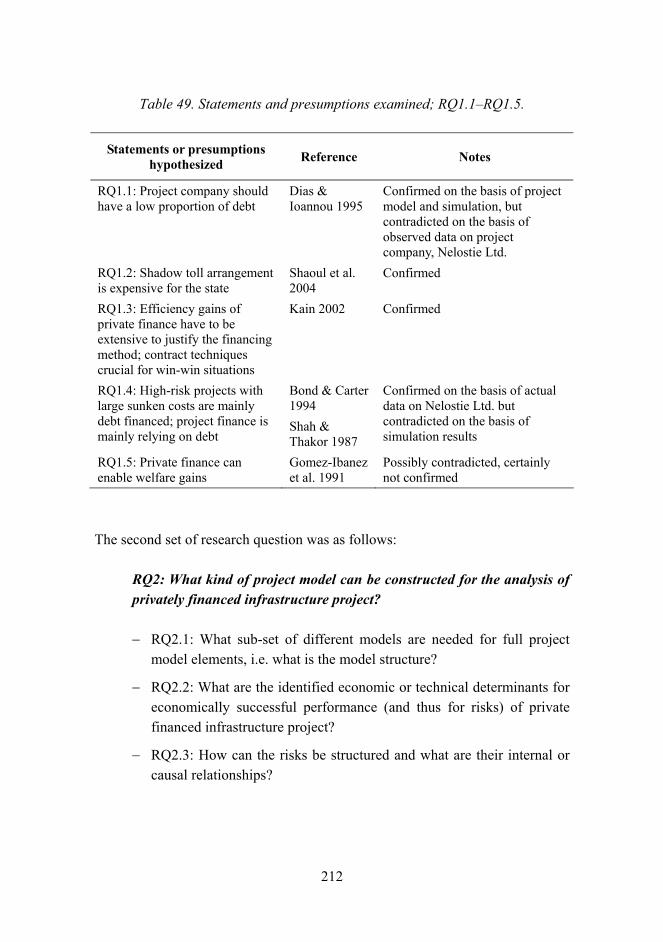
212

Table 49. Statements and presumptions examined; RQ1.1�RQ1.5.

Statements or presumptions hypothesized Reference Notes

RQ1.1: Project company should have a low proportion of debt

Dias & Ioannou 1995

Confirmed on the basis of project model and simulation, but contradicted on the basis of observed data on project company, Nelostie Ltd.

RQ1.2: Shadow toll arrangement is expensive for the state

Shaoul et al. 2004

Confirmed

RQ1.3: Efficiency gains of private finance have to be extensive to justify the financing method; contract techniques crucial for win-win situations

Kain 2002 Confirmed

RQ1.4: High-risk projects with large sunken costs are mainly debt financed; project finance is mainly relying on debt

Bond & Carter 1994 Shah & Thakor 1987

Confirmed on the basis of actual data on Nelostie Ltd. but contradicted on the basis of simulation results

RQ1.5: Private finance can enable welfare gains

Gomez-Ibanez et al. 1991

Possibly contradicted, certainly not confirmed

The second set of research question was as follows:





213

The primary result will be a model of the case project which then will be analysed using simulation to derive possible outcomes of the project and outcomes for project investors. This project model includes several elements or sub-models:

Risk structure model identifies relevant project-specific (or internal) risks and wider, external risks such as macro-economic risks. This model was derived from the literature and synthesising several research findings. The model is unique and not presented as such or in such format before. This model was shown in Figure 7.

Risk structure model must evidently be operationalized and risk relationships of observable and accessible risk parameters, because risks are not isolated from each other but in most cases associated with each other, they must be linked by logical relationships. Most often these links are dynamic (bi-directional), but for modeling purposes the causal order is not relevant. These parameters are also the basis of cash flows and thus affect the project�s economic outcomes; this sub-model was called the project framework model and was presented in Figure 20 and in equations Eq.7-6�Eq.7-9 thus taking a multi-equation form.

The cash flow and valuation model adopts the standard tools of corporate finance. This model looks equally at all stakeholders� cash flows, not only the investors�. This model was depicted by equations Eq.4-6�Eq.4-16 complemented by cost of capital models Eq.4-17�Eq.4-19.

For investigation of different possible states-of-the world, a scenario producing model was constructed. The economic growth time series model generated different states-of-the-world (or rather states-of-the-project) and used the risk parameters� relationships to derive cash flows leading to different possible economic outcomes of the project.

Finally, the full project model includes cash flows of the project in addition to the abovementioned sub-models using Eq.8-2�Eq.8-5.

As an answer to RQ2.1 it is possible to illustrate the model structure as a whole, as shown in Figure 39. The model hierarchy shows how different modelling

214

levels are needed in order to construct a sound project model and how the models must be operationalized from conceptual levels to quantitative models. However, one of the key conclusions of this research is that going straight to the quantitative level does not produce a logical whole. Without the conceptual level the model would most likely miss e.g. the relationships between risk and value determinants of the project. The result would be isolated analyses of particular viewpoints missing the systems view.

Projectmodel

Project frameworkmodel

Mac

ro-e

cono

mic

scen

ario

s

Project cash flows

and cost of capital

Risk

structure

model

Risk

structure

mod

el

Projectmodel

Project frameworkmodel

Mac

ro-e

cono

mic

scen

ario

s

Project cash flows

and cost of capital

Risk

structure

model

Risk

structure

mod

el

Figure 39. Project model and its sub-model components � RQ2.1.

RQ2.2 stated the research question on the determinants of the economic performance of the project. We have to separate here the different views of the state and the investors as well as different time horizons where risks profile changes. For investors, the risk chart shown in Figure 40 illustrates what risks are deemed critical and which risks are highly associated with each other.

215

Capital structure forms the main risk for liquidity of the project company and further to equity investors. If the project company goes insolvent, the debt financiers or the state might step in and take over the project and concession � and finally the equity investors could lose their capital investment in the project company. Capital structure risk is naturally the consequence of high interest rates against which the concessionaire has hedged his/her investment. But notwithstanding, the risk is there regardless of the hedging scheme. In fact, explanatory power of capital structure (high debt) risk was about 50% (0.501) in simulated insolvency situations.

Low traffic was forming the main long-term risk (value risk) with explanatory power of 0.589 in simulated NPV_PI (net present value of project investors� investment) outcomes. Thus, about 60% of the NPV_PI values were explained as a consequence of low traffic growth. Low traffic is naturally explained mainly by low economic growth in general.

Capital structure(high debt)

Low traffic

High inflation

High operating cost

Low traffic

High interest rates

Low economic growth

Medium/short term(= insolvency risk)

Long term(= value risk)

High risk=high prioritydeterminant

Low risk=low prioritydeterminant

I n v e s t o r h o r i z o n

R i s k p r i o r i t y

Capital structure(high debt)

Low traffic

High inflation

High operating cost

Low traffic

High interest rates

Low economic growth

Medium/short term(= insolvency risk)

Long term(= value risk)

High risk=high prioritydeterminant

Low risk=low prioritydeterminant

I n v e s t o r h o r i z o n

R i s k p r i o r i t y

Figure 40. Risk determinants, their relationships (dashed arrow lines) and the term structure � RQ2.2, RQ2.3 and RQ3.1.

216

The other risks � higher than expected inflation, operating cost, and interest rates as well as low economic growth are then more or less contributing to the abovementioned high priority risks. However, since the causal impact of these low priority risks are so evident, they must be included in the analysis and in fact they are the reason behind the high priority risks. Figure 40 indicates the dynamics between risk determinants and highlights the importance of systems view to risks. Sensitivity analysis alone and/or isolating the risk determinants could dilute the priorities and understanding of the causality.

The first part of the third research question is addressed to shareholder wealth problem of project investors and thus RQ3.1 (Which risk determinants most affect the project�s and investors� economy and what seems to be their ranking?) is linked with RQ2.2 of risk determinants. Hence, Figure 40 is the answer to RQ3.1 as well.

The latter part of RQ3 (What is the economic performance of the case project?) was stated as

− RQ3.2: What is the state�s position with regard to project economy and how well do state�s and project investors� interests coincide?

To this question a straightforward answer can be given: the state�s and project investors� interests do not coincide easily. Only in those cases, where the project is highly socio-economically profitable and has to be prioritized because of strategic reasons without having to commit state�s funds to the construction, the interests might have a common cross section point. As such, private finance does not seem to be economical for the state. This is visible from Figure 41, where the explicit answer to RQ3.2 is illustrated. Bs/Cs denotes the total benefits and costs ratio for the state when taking into account the socio-economic benefit cost ratio (B/C) of the project as well as the tax revenues received and toll payments paid by the state, as was explained in Chapter 10.8.44 The state�s total benefits and costs can be compared by looking at shadow tolls to be paid (cost to the state) and socio-economic benefits and tax revenues received (benefits for the state). So the benefit-cost ratio for the state depends on these variables. The analysis of Chapter 10.8 and visualisation of Figure 36 has been developed further in Figure 44 See Table 44, Eq. 9-12 and Figure 36.

217

41. It shows that project investors� return (including both debt and equity investors) increases in accordance with unit tolls received by the project company. Investors� return is a single curve as a function of unit toll and is totally independent from socio-economic return and related issues. Vice versa, the state�s costs rise as unit tolls increase. The state�s benefits are mainly dependent on the socio-economic benefits generated by the project with some adding to benefits through tax revenues paid by the project company. The state�s return curves depend likewise on unit toll that has to be paid and the curves are drawn for projects45 with different socio-economic cost-benefit ratios.

Figure 41 shows the curves of private investors� return (as a benefit-cost ratio for their investment) and the benefit-cost ratio of shadow toll arrangement for the state as a function of selected unit toll and when assuming different socio-economic benefit-cost ratios for the project. The interpretation comes when looking at the intersection points of the return (benefit-cost) curves. The investors� and the state�s interests do not coincide unless the socio-economic benefit-cost ratio exceeds value 2.5. Beyond that value, it could be expected that investors� return curve and Bs/Cs curve have an intersection point which is above value 1 for both parties, i.e. a potential win-win point.

45 Alternative, hypothetical socio-economic benefit-cost ratios for identical projects as the case project.

218

0

0,5

1

1,5

2

2,5

0,3 0,5 0,7 0,9 1,1

Unit toll (FIM / Project vehicle kilometres of travel)

Ret

urn

on p

roje

ct (s

tate

's an

d in

vest

ors')

Investors' return onproject

Bs/Cs w hen B/C=2,5

Bs/Cs w hen B/C=2,2

Bs/Cs w hen B/C=1,6

Bs/Cs w hen B/C=1,0

Figure 41. Project returns to the state and investors – RQ3.2; Bs/Cs is the state’s return in shadow toll arrangement and B/C is the socio-economic benefit-cost ratio.

The methodological validation can be done only in a preliminary way. As there are no empirical data to such an extent that would allow a large sample of privately financed projects to be analyzed in view of their full life cycle, the only method is to do time-wise cross-sectional analysis and/or simulation of projects. The use of simulation results as a statistical data is done often in situations where empirical data is missing or when empirical sampling and observation is too resource consuming. However, the results are only as good as the simulation models are. In this research, the preliminary diagnostics showed that simulation errors, i.e. the comparison between actual observations and simulation results of project company data, are surprisingly tolerable. Therefore, it is concluded that the model developed as one of the results in this research is well worth applying and developing further. Using more recent data and future observations of the case project company, it is possible to adjust the model so that it even better describes the financial results of the project company. The model is very well fitted for strategic ex ante evaluation of similar projects and as a part of corporate business planning when the corporation is in project finance business. The conceptual level model can also be fitted to different environments, such as different countries, different branches of industries, etc. once the calibration of

219

the model is done using appropriate empirical data to build relationships between economic variables and cash flow components.

The results of this research clearly put forward a question about claimed benefits of private finance. The results seem to point to the opposite direction: private finance is expensive and its presumed benefits need to be extensive in order to justify alternative finance methods to traditional construction and maintenance bidding process. However, we should constantly keep in mind that the case project was a novelty in Finland and the market for such a project is still undeveloped in terms of experience and knowledge. Also it is noteworthy, that the case project was completed well ahead of the planned schedule, resulting in gains for investors in the form of advanced cash flows but also to the society in the form of advanced socio-economic benefits. The net result showed in Figure 41 would not change because of these facts nonetheless.

In light of actual observations on the project company�s data it seems that not all investors had access to all the relevant information concerning project risks and thus their wealth seems not have been maximized so far. Of course, the concession term is only at the midway point and nothing definite can be said about the final performance of the project company.

15.2 Validation of the research approach and some generalized findings

There are a number of viewpoints that can be taken in the validation of the research process: the data, the modeling and simulation approach, the context of applicability and the methodological choices in general, just to name some. In this chapter, some of these issues are selected in order to validate the research approach. Also the generalized results are presented at the end of this chapter, because the generalization potential is very much dependent on the validity of the research approach.

The data that was used in the modeling of the project was strictly empirical. This can be mentioned as a virtue. The weakness, however, was the fact that some of the time series were short (e.g. for interest rate rH the n = 9) which undermines the credibility of regressed associations. In most cases, luckily, the time series

220

were reasonably well covering the historical behavior of the variable in question, so this weakness of short time periods of empirical material is only in the abovementioned individual point and definitely not throughout the study. For the most part, the empirical material covered the time between 1980�1995, i.e. n = 16.

The empirical data for modeling was prior to 1995, because in 1996 was the time for decisions on the project. Thus, the modeling effort reflects the decision making point of that time. The model itself, built on empirical data, is however most suited for ex ante analysis of projects and thus it serves as a decision making tool in order to analyze projects. For empirical analysis of similar projects, we only need the observed data, not models. One of the merits of the model is that it is modularly structured and built and that it is easily updated with more recent empirical data. The modular structure serves as a starting point for similar models aimed at appraisal of other types of private finance infrastructure projects. Outside infrastructure sector, the model is hardly applicable at all.

The case being that empirical material concerning privately financed projects is hard to summarize in a uniform manner and because many of these projects are still ongoing and uncompleted, the final empirical experiences will have to wait. In some respects, the modeled or simulated outcomes contradicted with empirical observations. This was particularly evident with regard to capital structure of the project company. The constructed model, as well as literature based on similar models, suggests that the project company should be mainly equity financed whereas the empirical observations concerning the case project and in general seem to suggest the opposite. Clearly, the classical corporate finance theory is missing something here. In regard to model performance in general, the results of the model were satisfactory at least, indicating that the model can be used and developed further.

The model was based on simple linear relationships between the economic and project variables. Thinking of the model performance this was probably a good and applicable solution. However, the econometric finesses are bypassed and only very brief arguments are presented to justify the relationships. These arguments are based on basic economics literature. The model could well be further refined by incorporating more sophisticated econometric relations and e.g. extending beyond linear relationships. There is nothing that hinders this.

221

Of paramount importance is the fact that the research approach was carried out within the scope of the research questions. In other words, the aim was neither to construct a perfect project model nor to justify or object private finance as such, but to analyze the risks of a privately financed road project especially from the viewpoint of private investors. These results are then reflected more generally to the question of how and in what conditions private finance could successfully be employed. Here the risk is the volatility or uncertainty of certain variables and through them the uncertainty of economic outcomes. Risks are not independent, but in complex interaction with each other and the idea was to point out which risks are more relevant than others. In achieving this, the research approach served well. Aside from modeling and simulation it is hard to see alternative ways how to analyze this problem in present situation with the lack of empirical experiences.

The risks of the project are always priced if they are acknowledged and one of the key findings was through risk analysis to evaluate how successful private finance could be in similar projects. This was an obvious outcome of the research and as such of critical importance to finance policies for infrastructure. If the private sector prices the risks and if the public sector does not, the question of risk transfer becomes somewhat pointless. The state has to pay extra for the risks of private investors but not for the risks it willingly assumes itself. Each project is unique especially in the eyes of private investors, whereas the state is probably more inclined to see a portfolio of projects. This is due to number of reasons, one certainly being the mere size of major infrastructure projects. Private investors want to ensure positive net present value for their investment with reasonable certainty whilst the state can survive if in average all the projects – but not necessarily every single one – in its portfolio are successful.

The role of contracts and negotiation process cannot be overemphasized. While the risks can be hedged, negotiated, shared, and so forth, the risks are always there and the question is how they are juggled between negotiating parties. As this view of the private finance is emphasized, the significance of information on risks is underlined at the same time. If there are differences in the level of knowledge on and understanding of risks, there is an opportunity for extra gains through sole negotiation tactics and contract formulation. This research can contribute to this process, thinking of all negotiating parties: the investors, both debt and equity, and the state. When the level of information is equal to all parties, the negotiation process is likely to yield to an acceptable and fair

222

outcome. The weakness in this research was that the contract terms were not known in detail leading to assumptions, simplifications and robust handling of some risks. Nevertheless, the analysis of detailed contractual arrangements would be a story of its own and certainly something for further research. This research can help in setting up such research efforts. But each project is unique in many ways, as will the appropriate contract formulations be, so that this type of research can contribute only to a limited extent.

What can be said in general about contracts based on the experience of this research? First, the contracts should be clear cut in a manner that the level of detail is very limited and that the details do not become a major issue. Complex contracts do not mean that all issues are adequately covered but rather could be a signal that the overall framework is poorly defined. Secondly, it should be the state that sets the framework as clearly as possible because comparing contracts is not really what should be in the minds of state representatives but rather comparing the bids on a uniform basis. Too much leeway in the formulation of calls of bids and leaving too many details for the negotiation process will result in more efforts to be taken in this process and leaves too many options open, so that the negotiation process becomes the definition of the project contract itself.

Returning to the original question of value and risk of privately financed infrastructure projects, based on this research we can say that the private investors can gain additional value when financing these projects, but it comes with a price, which is always paid by the taxpayers (as in shadow toll arrangement) or users (as in user toll arrangement). The efficiency gains (productivity, earlier supply of the service or facility, and so on) must exceed the price paid for private capital and this equation is not always easy to solve. Mega-projects with mega-class risks will inevitably include “mega-risk premiums” which are paid by somebody, whether the risks go off or not. However, the long-term value risk is not perhaps that severe in long-life infrastructure projects that have quite low volatility in terms of cash flows. They could be excellent projects in large-scale capital investors’ portfolio.

Table 50 attempts to summarize the strengths and weaknesses of the adopted research approach and derived models as well as the potential for generalization of the main findings. Many of the weaknesses or shortcomings can be overcome.

223

Table 50. The merits and shortcomings of the research and significant findings.

Strengths, merits or significant findings Weaknesses, shortcomings or restrictions

Applicability on similar infrastructure projects, e.g. airports, rail lines, harbors, etc.

Not applicable to private finance projects in general

Modular structure to be applied at different levels

Sensitivity to lack of data

Ability to address dynamic relations between selected variables

Incapability to address contractual issues effectively

Reliance on corporate finance theories Lack of econometric sophistication Updatable with more recent empirical data Requires a lot of data Suitable for ex ante analysis Not well suited for ex post analysis

Models

Good or satisfactory performance of the model

Combining several fields of research (finance, transport, economics)

Not focused on single research field and brief on econometric analysis

A novel approach to build a project model and simulate the project company

Empirical part restricted to models

Model diagnostics Short on contractual analysis Clear contribution to the field of finance of transport infrastructure and an applicable approach for other infrastructures, e.g. airports, rail lines and harbors

Research approach

Holistic view to value and risks of privately financed infrastructure project

Findings on the price of private finance; the price is high, but in selected cases (good, urgent projects) could be tolerable

Exact comparison mechanism presented only for the case project

The rough risk structure of a shadow toll road project; the basic structure can be generalized for any transport infrastructure project

Risk structure and argumentation limited to transport infrastructure

Some policy recommendations were enabled based on the case analysis

Policies restricted to transport infrastructure, not private finance in general

Private investors� relevant risk determinants in the case project and in similar projects; the relevance and prioritization of different risks and their term structures

Not all risks were covered

Generalized findings and contributions

Corporate finance theory based solutions on optimal project company capital structure contradict with empirical observations

Some other theories could explain better the capital structure choices, but these were not investigated

224

15.3 Further research needs

One of the clear further research needs identified is quantitative, empirical research concerning the benefits of alternative finance methods. Too often the “research” on these issues is merely logical reasoning of presumed benefits and impacts of novel finance methods. For these research issues, empirical material must be gathered from several projects. In the UK, such a number of projects will soon, if not now, be available. But, as this research shows, each project is idiocratic and context-specific. This was proven by showing that project-specific demand was the most relevant risk factor concerning project’s economic performance. This in turn leads us to the conclusion that certain typologies for successful (or unsuccessful) projects financed with private capital could be researched if the projects in themselves and in the end are idiocratic. However, such a research is very ambitious because of varying frameworks concerning economy, type of project, risks, etc. and this type of research would require truly extensive resources – if at all possible. Probably the most feasible approach would be to combine several case analyses, such as this research, and building a pool of knowledge on privately financed projects. Such an approach would most likely require co-operative efforts of international finance institutions (World Bank, European Investment Bank, Asian Development Bank, etc.), national governments and researchers.

The methods of project economy evaluation should be developed further too. This research shows that the basic tools, such as discounted cash flows, net present value analysis and CAPM can be combined in various ways and with fruitful results. However, the optimal tool set selection seems to be very contingent and sometimes probably a matter of coincidence, taste and personal abilities of the investigators. The model structure presented as a result of this research (RQ2.1) already sets a framework for model components and the methods. Clearly, project evaluation methods, cash flow accounting and value analysis as well as basic econometric models are those that can be integrated to serve advanced project appraisal in terms of financial, contractual and organisational arrangements. Some sort of simulation models are certainly needed for aiding project investment related decisions. The model structure offered by this research is one possible starting point. Also the employment of option theory in case of real operating and decision options can be an area where new knowledge can be found. Project decisions always contain several real and

225

operating options and the valuation tools can be very complex for the investigators to apply. Making the application easier would certainly improve the quality of decisions.

A clear need for further research is concerning contractual arrangements, which were only briefly handled by this research. A more focused analysis of contractual issues would help the future projects to be built on sustainable and fair contracts. However, the research should be more oriented towards the contractual architecture rather than on analysis of details.

226

References

Albon, R. (1995). Efficient access charging in rail. Road & Transport Research, Vol. 4, No. 3, September 1995, pp. 18�26.

Altman, E. (1984). A Further Empirical Investigation of the Bankruptcy Cost Question. Journal of Finance, Vol. 39, No. 4, Sep 1984, pp. 1067�1089.

Aschauer, D. (1989). Is Public Expenditure Productive? Journal of Monetary Economics, Vol. 23, March 1989, pp. 177�200.

Bank of Finland (1986�1996). Monthly bulletins from 1986�1996.

Berry, W.D. & Feldman, S. (1985). Multiple Regression in Practice. Sage University Paper. Series in Quantitative Applications in the Social Sciences. Beverly Hills/London/New Delhi.

Bodie, Z. & Rosansky, V. (1980). Risk and Return in Commodities Futures. Financial Analysis Journal, May�June 1980.

Bogue, M.C. & Roll, R. (1974). Capital Budgeting of Risky Projects with �Imperfect� Markets for Physical Capital. The Journal of Finance, Vol. 29, No. 2, May 1974, pp. 601�613.

Bond, G. & Carter, L. (1994). Financing Private Infrastructure Projects. International Finance Corporation. Discussion Paper no 23, 1994, pp. 10�11.

Borins, S.F. (1981). The Effect of Pricing Policy on the Optimal Timing of Investments in Transport Facilities. Journal of Transport Economics and Policy, May 1981, pp. 121�133.

Brealey, R.A. & Myers S.C. (1991). Principles of corporate finance. McGraw-Hill.

227

Brealey, R.A., Cooper, I.A. & Habib, M.A. (1996). Using Project Finance to Fund Infrastructure Investments. Journal of Applied Corporate Finance, Vol. 9, No. 3, Fall 1996, pp. 25�38.

Button, K.J. (1994). Alternative Approaches Toward Containing Transport Externalities: An International Comparison. Transportation Research A, Vol. 28, No. 4, July 1994, pp. 289�305.

Byrns, R.T. & Stone G.W. (1997). Economics. 6th edition. Harper Collins College.

Constantides, G.M. (1978). Market Risk Adjustment in Project Valuation. The Journal of Finance, Vol. XXXIII, No. 2, May 1978, pp. 603�616.

Copeland, T.E. & Weston, J.F. (1988). Financial Theory and Corporate Policy. 3rd edition. Addison Wesley.

Damodaran, A. (2005a). Damodaran�s web pages http://www.damodaran.com, paper �Valuing Private Firms�, read January 26, 2005.

Damodaran, A. (2005b). Damodaran�s web pages http://www.damodaran.com, The Data Page, Ratings, Spreads and Interest Coverage Ratios, read January 26, 2005.

Damodaran, A. (2005c). Damodaran�s web pages http://www.damodaran.com, Finding the Right Financing Mix: The Capital Structure Decision, read January 26, 2005.

DeAngelo, H. & Masulis, R.W. (1980). Optimal Capital Structure under Corporate and Personal Taxation. Journal of Financial Economics, Vol. 8, No. 1, pp. 3�29.

Dias, A. & Ioannou, P.G. (1995). Debt Capacity and Optimal Capital Structure for Privately Financed Infrastructure Projects. Journal of Construction Engineering and Management, Vol. 121, No. 4, Dec 1995, pp. 404�414.

Doherty, N.A. (1985). Corporate Risk Management: A Financial Exposition. McGraw-Hill.

http://www.damodaran.com



228

Doyle, J. & Falter, D.C. (1985). Highway Bond Financing, 1962�1982: An Examination. Trans Res Rec 1009. Washington DC.

Eichengreen, B. (1995). Financing Infrastructure in Developing Countries: Lessons from the Railway Age. The World Bank Observer, Vol. 10, No 1, Feb 1995, pp. 75�91.

European Conference of Ministers of Transport (1990). Private and Public Investment in Transport. Economic Research Centre. Paris.

Euske, K.J. (1984). Management Control: Planning, Control, Measurement, and Evaluation. Addison-Wesley Publishing Company.

Fayard, A. (1993). Toll Financing, Risk Financing. How to Fit the Needs without Dogmas. The French Experience. Conference Paper. The East European Road Conference, Warsaw 22�24 September, 1993.

Fielding, G.J. & Klein, D.B. (1993). How to Franchise Highways. Journal of Transport Economics and Policy, Vol. 2, No. 27, May 1993, pp. 113�130.

Finnish Road Administration (1990). Tienpidon tehtävä- ja suoriteryhmittely [Road Construction and Maintenance Cost Codes]. Helsinki. (In Finnish only.)

Finnish Road Administration (1991). Kustannusarvioiden pysyvyys, vuoden 1990 tulosraportit [Stability of project cost estimates, report on attaining goals for 1990]. Internal memorandum drafted by Timo Hiltunen March-3-1991. (In Finnish only.)

Finnish Road Administration (1992). Tulosraportti 1991 [Finnra report of attaining goals for 1991]. Helsinki.

Finnish Road Administration (1993). Tie- ja siltapäällysteiden urakkahinnat vuonna 1993 [Road and bridge pavement contract prices in 1993]. Helsinki. English abstract provided.

Finnish Road Administration (1995a). FinnRA statistics 1995. Helsinki.

229

Finnish Road Administration (1995b). The Road Traffic Forecast for 1995�2020. Helsinki.

Finnish Road Administration (1995c). Päällystystyöt 1995 [Paving works 1995]. Helsinki. (In Finnish only.)

Finnish Road Administration (1995d). Tieliikenteen ajokustannukset 1995 [Costs of Road Traffic 1995]. Helsinki. (In Finnish only.)

Finnish Road Administration (1996a). Yleisten teiden tuotantotilasto 1995 [Production Statistics for Public Roads 1995]. Tielaitoksen tilastoja 2/1996 [Finnra statistics series 2/1996]. Helsinki. (In Finnish only.)

Finnish Road Administration (1996b). Tiepäällysteet 1.1.1996, Päällystystyöt 1995 [Pavements 1.1.1996, Pavement Production Statistics 1995]. Helsinki. (In Finnish only.)

Finnish Road Administration (1996c). Upgrading main road 4 Järvenpää�Lahti to motorway by private finance. Project brochure, Finnish Road Administration, Helsinki.

Gomez-Ibanez, J.A., Meyer, J.R. & Luberoff, D.E. (1991). The Prospects for Privatising Infrastructure. Journal of Transportation Economics and Policy, Vol. 25, No. 3, Sep 1991, pp. 259�277.

Griffith-Jones, S. (1993). Loan Guarantees for Large Infrastructure Projects. Commission of the European Communities. Luxembourg.

Griffith-Jones, S. (1995). Loan Guarantees for Large Infrastructure Projects: The Issues and Possible Lessons for a European Facility. Office for Official Publications of the European Communities. Pp. 13�14.

Hair, J.F. Jr, Anderson, R.E., Tatham, R.L. & Black, W.C. (1998). Multivariate data analysis. New Jersey: Prentice-Hall.

230

Haley, G. (1992). Private finance for transportation and infrastructure projects: a view. International Journal of Project Management, Vol. 10, No. 2, May 1992, pp. 63�68.

Helm, D. & Thompson, D. (1991). Privatised Transport Infrastructure and Incentives to Invest. Journal of Transport Economics and Policy, Vol. 25, No. 3, Sep 1991, pp. 231�246.

Hemmilä, P. & Kankainen, J. (1993). Maarakennuskustannusindeksi 1990 = 100 (Civil Engineering Works Cost Index 1990 = 100). Statistics Finland handbooks 32. Helsinki: Statistics Finland.

Hong, H. & Rappaport, A. (1978). Debt Capacity, Optimal Capital Structure, and Capital Budgeting Analysis. Financial Management, Vol. 7, No. 3, Autumn 1978, pp. 7�11.

Howard, J.A., Rivkin, G., Brecher, S. & Heder, L. (1985). Strategies to Implement Benefit-Sharing for Fixed-Transit Facilities. Transportation Research Board.

Hsia, C.C. (1981). Coherence of Modern Theories of Finance. Financial Review, Winter 1981, pp. 27�42.

Ingersoll, J. & Ross, S. (1992). Waiting to invest: investment and uncertainty. Journal of Business, Vol. 65, No. 1, January 1992, pp. 1�29.

Johansen, F. (1989). Toll Road Characteristics and Toll Road Experience in Selected South East Asia Countries. Transportation Research, Vol. 23A, No. 6, p. 464.

Kain, P. (2002). Attracting Private Finance for Infrastructure Projects: Lessons from the Channel Tunnel Rail Link. International Journal of Transport Economics, Vol. XXIX, No. 1, February 2002.

Kallunki, J.-P., Martikainen, T. & Niemelä, J. (2001). Yrityksen arvonmääritys (Valuation of the Firm). 2nd ed. Helsinki: Kauppakaari.

231

Kangari, R. (1995). Risk Management Perception and Trends of U.S. Construction. ASCE Journal of Construction Engineering and Management, Vol. 121, No. 4, December 1995, pp. 422�429.

Kay, J. (1993). Efficiency and Private Capital in the Provision of Infrastructure. Infrastructure Policies for the 1990s. Paris: OECD. 67 p.

Kendall, M.G. (1973). Time-Series. 1st edition. London: Griffin.

Khan, A.M. & Fiorino, D.P. (1992). The Capital Asset Pricing Model in Project Selection: A Case Study. The Engineering Economist, Vol. 37, Winter 1992, pp. 145�159.

Kim, E.H. (1978). A Mean-Variance Theory of Optimal Capital Structure and Corporate Debt Capacity. Journal of Finance, Vol. 33, No. 1, pp. 45�63.

Koskenkylä, H. (ed.) (2002). Suomen rahoitusmarkkinat 2002. Suomen Pankki, Tutkimuksia A:102. Helsinki: Bank of Finland.

Kuschel, S. (1995). Private Finance for Transport Infrastructure in Central and Eastern Europe Countries. Too Good to be True? Routes&Roads No 286-I-1995.

Lave, C. (1994). The Demand Curve under Road Pricing and the Problem of Political Feasibility. Transportation Research Part A, Vol. 28, No. 2, pp. 83�91.

Lawson, G.H. & Stark, A.W. (1975). The Concept of Profit for Fund Raising. Accounting and Business Research. Winter 1975.

Leviäkangas, P. (1996). Bomvägfinansiering i Norge. Några generalla fakta och två projektbeskrivningar från Syd-Tröndelag med vikten på bominkrävning, finansiering och ekonomi. [Road toll financing in Norway. Some general facts and two case studies from Trondheim region with emphasis on toll collecting and project financing]. Internal publications of Finnish Road Administration 37/1996. In Swedish.

232

Leviäkangas, P (1998). Determination of the market value of a privately financed infrastructure project � Case of Järvenpää�Lahti motorway. International Symposium on Road Financing � Construction, Maintenance and Operation, Paris 4�6 November 1998. IRF, PIARC, World Bank and Ecole nationale des Ponts et Chaussees. Pp. 323�332.

Leviäkangas, P. & Lähesmaa, J. (2002). Profitability Evaluation of Intelligent Transport System Investments. ASCE Journal of Transportation Engineering, Vol. 128, No. 3, May 1, 2002.

Leviäkangas, P. & Talvitie, A. (2004). Cost Recovery on Finnish Public Roads. 10th World Congress on Transportation Research, July 4�8, Istanbul 2004. Proceedings cd-rom.

Lipsey, R.G. & Chrystal, K.A. (1995). An Introduction to Positive Economics. 8th ed. Oxford University Press.

Lockwood, C.L. et al. (1992). Highway Finance: Revenues and Expenditures. Transportation Research Record, No. 1359, pp. 11�18.

Markowitz, H. (1959). Portfolio Selection: Efficient Diversification of Investments. New Haven: Yale University Press.

McLeod, A.I. & Sales, P.R.H. (1983). An algorithm for approximate likelihood calculation of ARMA and seasonal ARMA models. Applied Statistics, Vol. 32, No.2, pp. 211�223.

McMillan, C. & Gonzales, R.F. (1973). Systems Analysis. A Computer Approach to Decision Models. 3rd ed. Illinois: Richard D. Irwin, Inc.

Mendenhall, W. & Sincich, T. (1992). Statistics for Engineering and Sciences. 3rd ed. Dellen: San Francisco.

Mills, G. (1991). Commercial Funding of Transport Infrastructure. Lessons from Some Australian Cases. Journal of Transport Economics and Policy, Vol. 25, No. 3, Sep 1991, pp. 279�298.

233

Mills, G. (1995). Welfare and Profit Divergence for a Tolled Link in a Road Network. Journal of Transport Economics and Policy, Vol. 29, May 1995, pp. 137�146.

Ministry of Transport and Communications (1994). Liikenteen väylähankkeiden vaikutusselvitysten yhdenmukaistaminen [Harmonisation of infrastructure project impact anlyses]. Publications 26/94. Helsinki.

Ministry of Transport and Communications (1995a). Private Finance for Roads. Publications by the Ministry of Transport and Communications L17/95. Helsinki.

Ministry of Transport and Communications (1995b). Finnish transport infrastructure 2010. Ohjelmia ja strategioita 4/1995. Helsinki.

Ministry of Transport and Communications (2006). Long-term sustainability in decisions about transport infrastructure. Publications of Ministry of Transport and Communications 18/2006. Helsinki.

Mitchell, J. & Hill, T. (1992). The Limits to Developer Contributions: An LRT Case Study. Seminar Paper. Proceedings of seminar C held at the PTRC European transport, highways and planning, 20th Summer Annual Meeting, September 14�18, 1992. Volume P355. Pp. 267�272.

Mohring, H. (1965). Characteristics of an Optimum Transportation System in a Competitive World. (In Measuring the Benefits of Government Investments, ed. Dorfman R.) Washington DC: Brookings Institution.

Morris, P.W.G. (1991). The Strategic Management of Projects. In: Male & Stocks (eds.). Competitive Advantage in Construction. Heriot-Watt University, Department of Building Engineering and Surveying.

Munnell, A.H. (1993). An Assessment of Trends in and Economic Impacts of Infrastructure Investment. Infrastructure Policies for the 1990s. Paris: OECD. Pp. 21�50.

Nelostie Ltd. (1998). Annual Statements from 1997. National Board of Office of Patents and Registeration.

234







Nevitt, P.K. & Fabozzi, F.J. (1995). Project Financing. 6th ed. Rochester: Euromoney Publications.

Newbery, D. (1994). The Case for a Public Road Authority. Journal of Transport Economics and Policy, Vol. 28, No. 3, September 1994, pp. 235�253.

Nilsson, J.-E. (1990). Private Funding of Public Investments. A Case of Voluntarily Funded Public Road. Journal of Transport Economics and Policy, Vol. 24, No. 2, May 1990, pp. 157�170.

Nilsson, J.-E. (1992). Second-Best Problems in Railway Infrastructure Pricing and Investment. Journal of Transport Economics and Policy, Vol. 26, No. 3, Sep 1992, pp. 245�259.

Niskanen, E. (1987). Congestion tolls and consumer welfare. Transportation Research B, Vol. 21B, No. 2, pp. 171�174.

Nordiska Ministerådet [Nordic Council of Ministers] (1996). Yearbook of Nordic Statistics 1996.

235

OECD (1994). Internalising the Social Costs of Transport. Paris.

Oum, T.H. & Tretheway, M.W. (1988). Ramsey Pricing in the Presence of Externality Costs. Journal of Transport Economics and Policy, Vol. 22, No. 3, Sep 1988, pp. 307�317.

Oum, T.H., Zhang, A. & Zhang, Y. (1996). A Note on Optimal Airport Pricing in A Hub-and-Spoke System. Transportation Research Part B, Vol. 30, No. 1, pp. 11�18.

Pajakkala, P. & Nippala, E. (2005). Väylänpidon lyhytjänteisten rahoitus-päätösten vaikutukset ja pitkäjänteisten hyödyt � asiantuntijalausunto [The impacts of short-term finance decision making and benefits of long-term finance decisions concerning transport infrastructure investments � an expert assessment]. Draft. August 18th, 2005. VTT, Tampere.

Pindyck, R.S. & Rubinfeld, D.L. (1991). Econometric Models and Econometric Forecasts. International Edition. Singapore: McGraw-Hill, Inc.

Potter, B.H. (1997). Dedicated Road Funds � A Preliminary View on a World Bank Initiative. IMF Paper on Policy Analysis and Assessment. International Monetary Fund.

Redhead, K. & Hughes, S. (1988). Financial Risk Management. Brookefield: Vt. Gower.

Ren, H. (1994). Risk lifecycle and risk relationships on construction projects. International Journal of Project Management, Vol. 12, No. 2, pp. 68�74.

de Richecour, A.B. & Heggie, I.G. (1995). African Road Funds: What Works and Why? Working Paper 14, SSATP, Africa Technical Department, World Bank. Washington DC.

Rothengatter, W. (1994). Do External Benefits Compensate for External Costs of Transport? Transportation Research A, Vol. 28, No. 4, pp. 321�328.

236

Salmi, T. & Virtanen, I. (1995). Deriving the Internal Rate of Return from the Accountant�s Rate of Return: A Simulation Testbench. Proceedings of the University of Vaasa, No. 201. Vaasa, Finland: University of Vaasa.

Salmi, T. & Virtanen, I. (1997). Measuring the Long-Run Profitability of the Firm; A Simulation Evaluation if the Financial Statement Based IRR Estimation Methods. Acta Wasaensia, No 54. Vaasa, Finland: University of Vaasa.

Shah, S. & Thakor, A.V. (1987). Optimal Capital Structure and Project Financing. Journal of Economic Theory, No. 42, pp. 209�243.

Shaoul, J., Stafford, A. & Stapleton, P. (2004). Highway Robbery? A financial analysis of Design Build Finance and Operate in roads in the UK. The EIASM International Conference on Accounting, Auditing and Management of Public Sector Reforms. 7�9 October 2004, Oslo, Norway.

Sharpe, W.F. (1963). A Simplified Model for Portfolio Analysis. Management Science, Vol. 9, No. 2, Jan 1963, pp. 277�293.

Sharpe, W.F. (1964). Capital Asset Prices: A Theory of Market Equilibrium under Conditions of Risk. Journal of Finance, Vol. 19, No. 3, Sep 1964, pp. 425�442.

Shoemaker, P.J.H. (1980). Experiments on decisions under risk: The expected utility hypothesis. Boston: Martinus Nijhoff Publishing.

Skjeseth, T.H. & Odeck, J. (1994). Toll Road Financing in Norway: Organisational Framework and Experienced Financial Difficulties. PTRC�s Summer Annual Meeting and Conferences (perspectives 3). Pp. 97�106.

Smith, G. (1985). Macroeconomics. New York: W.H. Freeman.

Statistics Finland (1990). Statistical Yearbook of Finland 1990. Helsinki.



237

Szymanski, S. (1991). The Optimal Timing of Infrastructure Investment. Journal of Transport Economics and Policy, Vol. 25, No. 3, Sep 1991, pp. 247�258.

The 2nd Workshop on Applied Infrastructure Research (2003). Regulation and Investment in Infrastructure Provision � Theory and Policy. 11 October, 2003, Berlin.

Thomadakis, S. & Usmen, N. (1991). Foreign Project Financing in Segmented Capital Markets: Equity Versus Debt. Financial Management, Vol. 20, No. 4, Winter 1991, pp. 42�52.

Tikka, K. & Särkkä, T. (1996). Vt 4, SRRK-projekti. Liikenne-ennusteiden riski-tarkastelu (Main Road 4, DBFO-Project. Risk Analysis of Traffic Forecasts). Unpublished consultation report, Matrex Ltd., 15th July 1996.

Tiong, R. & Yeo, K.T. (1993). Project financing as a competitive strategy in winning overseas jobs. International Journal of Project Management, Vol. 11, No. 2, May 1993, p. 82.

Tiong, R.L.K. (1995a). Impact of Financial Package versus Technical Solution in a BOT Tender. Journal of Construction Engineering and Management, Vol. 121, No. 3, Sep. 1995.

Tiong, R.L.K. (1995b). Competitive Advantage of Equity in BOT Tender. Journal of Construction Engineering and Management, Vol. 121, No. 3, Sep 1995.

TRB (1988). Public and Private Partnerships for Financing Highway Improvements. National Cooperative Highway Research Program Report 307. June 1988.

Treynor, J. (1961). Toward a Theory of the Market Value of Risky Assets. (Unpublished manuscript.)

Vartia, P. & Ylä-Anttila, P. (1996). Kansantalous 2021 [The Finnish economy 2021]. Tampere: Taloustieto.

238

Venäläinen, A. & Helminen, J. (1992). Talvikunnossapidon sääindeksi [Winter maintenance weather index]. Unpublished Finnish Road Administration report.

Verhoef, E. (1994). External Effects and Social Costs of Road Transport. Transportation Research A, Vol. 28, No. 4, pp. 273�287.

Verhoef, E. (1995). The Demand Curve under Road Pricing and the Problem of Political Feasibility. Transportation Research Part A, Vol. 29, No. 6, pp. 459�465.

Warner, J. (1977). Bankruptcy Costs: Some Evidence. Journal of Finance, Vol. 32, No. 2, May 1977, pp. 337�347.

Webb, D.C. (1991). Long-Term Financial Contracts can Mitigate the Adverse Selection Problem in Project Financing. International Economic Review, Vol. 32, No. 2, May 1991.

Yates, C.M. (1994). Toll Roads in Mexico and Argentina. Seminar paper in the 22nd European Transport Forum 12�16 September 1994. Pp. 17�29.

YSE (1995). Yleiset sopimusehdot [General contract terms].

Zhao, T. & Tseng, C.-L. (2003). Valuing Flexibility in Infrastructure Expansion. ASCE Journal of Infrastructure Systems, September 2003, pp. 89�97.

A1

Appendix A: Expected operating (maintenance) costs

Table A-1. Estimated expected operating costs of the case project; 1996 prices.

Costs in 1 000 FIM Year

(1) (2) (3) (4) (5) (6) (7) Total 1997 0 0 0 0 0 0 0 0 1998 1 050 0 140 210 160 0 400 1 960 1999 2 100 350 140 210 160 0 400 3 360 2000 2 550 0 180 310 260 250 400 3 950 2001 4 200 0 280 430 320 250 500 5 980 2002 4 200 0 550 620 320 250 500 6 440 2003 4 200 0 550 620 320 500 500 6 690 2004 4 200 6 200 550 620 320 500 500 12 890 2005 4 200 10 500 550 620 320 500 500 17 190 2006 4 200 2 200 550 620 320 500 500 8 890 2007 4 200 2 500 550 620 320 500 500 9 110 2008 4 200 2 500 550 620 320 500 500 9 190 2009 4 200 4 100 550 620 320 500 500 10 790 2010 4 200 0 550 620 320 500 500 6 690 2011 4 200 3 400 550 620 320 500 500 10 090 2012 2 100 4 100 440 310 250 500 500 8 200 Total 58 200 35 850 7 230 8 290 4 670 6 250 7 700 128 190

Columns:

(1) Winter maintenance; (2) Pavement Maintenance; (3) Landscaping, road side scarenging and cleaning; (4) Traffic management and control, signing; (5) Illumination; (6) Road marking; (7) Bridge maintenance.

B1

Appendix B: Project description46

B.1 General information (Finnish Road Administration 1996c)

A working group set up by the Ministry of Transport and Communications recommended in its final report, 26th of March 1996, that private finance would be implemented to road construction and maintenance by shadow toll option. The working group presented that the shadow toll option would be introduced. The concession contract covers upgrading the Järvenpää�Joutjärvi stretch of semi-motorway into motorway and maintaining this stretch (both the old and the new carriageway) for 15 years. The cost estimates excluding VAT were 550�590 MFIM for the construction and 10 MFIM annually for the maintenance.

The construction project included

− second carriageway of the motorway, 69.0 km − ramps of graded interchanges (8 pcs) and rest areas (5 pcs), 12.5 km − other public roads, 1.0 km − private roads, 7.0 km − 88 bridges − 8.5 km of noise barriers − 130 km of game fences − road lighting in graded interchanges, 15 km − 1.9 mill. m3 of soil cuts − 1.5 mill. m3 of rock cuts.

B.2 Financing

The concessionaire finances the detailed engineering, construction and operation (maintenance) of the project. The prospective concessionaires bid for the 15-year concession contract, and had an option to make alternative bids introducing longer contract periods and alternative toll charging systems. The concessionaire had a right to arrange the financing in any suitable and legal manner. The 46 All the information has been obtained from the preparatory and final contract documents that were available from Finnish Road Administration.

B2

amount of equity capital that was laid, affected the competitiveness of the bid, though. The concessionaires were eligible to seek financing from European Investment Bank (EIB). The maximum amount of loan granted by EIB is 50% of the total cost. The loan could be withdrawn gradually.

B.3 Tolling system

The state owner pays a �shadow toll� to the concessionaire according to traffic performance (vehicle kilometres of travel) on the road. The traffic is measured at two sites. The first site represents assumed homogenous traffic volume on a 30,2 km stretch and the second site 39,0 km. In case of exceptional situations, when traffic volumes are not recorded or traffic is blocked, the traffic counts of the previous year for the same period apply. Some special clauses have been included for special traffic days. In any case, the concessionaire faces practically no risk of counting equipment malfunction.

The cash flow from shadow tolls is received in four payments: end of March, end of July, end of September and end of December. The first three payments are based on the total payment of the previous year. At the end of December the payments are balanced according to real traffic volumes. Different types of vehicles are not distinguished � each vehicle, or rather vehicle kilometre, is equally worth. The owner has a right to withdraw the liabilities of the concessionaire to a third party, as long as these liabilities are due to operations connected to the concession contract.

The concessionaire must divide traffic performance into at least two, but at most four, bands. The first band is a fixed toll per vehicle km and the subsequent categories are additional payments on top of fixed toll.

B.4 Construction phase clauses of the contract

The owner was eligible to claim compensation when bad quality, workmanship or engineering is detected. Special emphasis was laid on the quality assurance procedures and quality control documents. The evaluation of quality was done mainly on the basis of contractor�s/concessionaire�s quality control documentation supplemented with inspections and sampling. If inspections or sampling showed deviations from accepted quality level and contractor�s own

B3

reports did not conform to the sampling or inspection results, the contractor paid a 50.000 FIM sanction for each event of non-conformance.

The construction costs were not indexed except for the paving works, where the market price of bitumen could have an impact on contract payments.

B.5 Operating phase

As with construction the operating quality is based on concessionaire�s own reports supplemented with inspections by sampling. The sanctions are the same as above. There are sanctions concerning blocked lanes due to repair works or similar.

The operating costs are indexed totally throughout the concession period using civil engineering works cost index. The re-paving works are also included in the operating costs.

B.6 Risk Allocation

The risk allocation is at many points according to general Finnish contract terms (YSE 1995) but some essential parts are shown in Table B-1.47 The list concentrates on the most important issues and is not exhaustive.

47 Source: Finnra. VT 4 (E75) Järvenpää�Lahti SRRK-project. English translation of risk matrix, drafted August 15th, 1996. Some risks presented here are not shown in the risk matrix draft but are defined in other contract documents.

B4

Table B-1. Risk allocation between concessionaire and owner.

Risk Concess-ionaire Owner Shared Notes, clarifications

Interest rates X Foreign exchange rates X Rise in commodity and input prices during construction

X* X** *Rise of prices leading to higher construction cost

**The market price of bitumen Volumes in construction X Additional work X Additional work subscribed

by the owner or work due to third party needs

Volumes in maintenance and reconstruction

X

Weather conditions X Rise in commodity and input prices during concession

X

Traffic volumes X Hand over of the road reserve

X The owner is unable to hand over the road reserve by the

agreed date Archeological findings, rare or protected flora or fauna

X

Owner�s delays X Unexpected accidents on the site

X

Difficult ground conditions of the old carriageway

X Such information on ground conditions that the

concessionaire was unable to check before and during the

bid preparation The effects of existing road on the design and construction of the new road

X

Force majeure X

B5

B.7 Tax Issues

The Finnish VAT and business and industry regulating laws presented a problem at the beginning of the project. The Central Board of Taxation (Keskusverolautakunta) gave out a resolution48 stating that the project consisted of two parts: first, the construction service part and secondly the maintenance service part. The Board decided that for the construction service the concessionaire would have to pay VAT and income tax for the whole project when the road was completed, i.e. opened for traffic. This would have meant a severe front-end loading of tax burden for the concessionaire. Furthermore, the Board regarded that the concessionaire would have to deduct interest on debt concerning the construction phase on those particular years that the interest was paid. This might lead to a situation where the concessionaire would not be able to fully enjoy the tax shield provided by debt.

Depreciating the project was also problematic. Tax laws made it possible to have a maximum 10 years depreciation period. Now the concession period was 15 years in minimum and this meant also that there was a chance of not benefiting depreciation tax shields to a full extent � the project could well result in loss over several subsequent years. The Central Board of Taxation adopted this view too. Both the VAT regulations and business and industry tax regulations were altered49 so that

− value added taxes were paid at the end of each years traffic counting period

− income taxes were paid also according to the above principle

− depreciation could be done according to straight-line principle during the concession contract period.

48 Resolution no 273/1996, dated October 21st, 1996. 49 Laws no. 1256 and 1257.

C1

Appendix C: Modeled and observed variables

C.1 Modeled and observed variables, t+1 year ahead modeling

Figures from C-1 to C-5 show how the full project model is able to forecast each critical variable (annual economic growth ∆GDPt+1, annual national traffic growth ∆VKTt+1, annual interest on risky debt rH t+1, inflation ct+1 and annual project traffic demand growth ∆VKTpt+1) of year t+1, based on observed data in year t, t running from 1996 to 2005 or 2004 depending on the availability of observed data. It is clearly visible that the model works reasonably well for all the other variables except for interest rate for risky debt. Finland�s joining to the European Monetary Union in 2002 changed the economic environment. This change started even earlier, as Finnish markka was tied to Euro with fixed rate at the beginning of 1999. Obviously, the actual change of economic environment started some years earlier when Union member states started their co-operation concerning monetary and economic policies. This change is visible from the interest rate time series. For other economic variables, the project model works surprisingly well.

-10,0

-5,0

0,0

5,0

10,0

15,0

1980 1985 1990 1995 2000

Year

GD

P a

nnua

l cha

nge

(%)

Historical, before project Observed, during projectModeled t+1, based on historical Upper 95% limit for modeledLower 95% limit for modeled

Figure C-1. GDP change, modeled t+1 year ahead vs. observations.

C2

-6,0-4,0-2,00,02,04,06,08,0

10,012,014,0

1980 1985 1990 1995 2000

Year

VK

T a

nnua

l cha

nge

(%)


Figure C-2. National VKT change, modeled t+1 year ahead vs. observations.

0,02,04,06,08,0

10,012,014,016,0

1980 1985 1990 1995 2000

Year

r H (%

)


Figure C-3. Annual interest rate for risky debt contracts, modeled t+1 year ahead vs. observations.

C3

-4,0-2,00,02,04,06,08,0

10,012,014,016,018,0

1980 1985 1990 1995 2000

Year

Ann

ual i

nfla

tion,

c (%

)


Figure C-4. Annual inflation of construction and maintenance (civil engineering index change), modeled t+1 year ahead vs. observations.

-15,0

-10,0

-5,0

0,0

5,0

10,0

15,0

1980 1985 1990 1995 2000 2005

Year

VK

T p, a

nnua

l cha

nge

(%)


Figure C-5. Annual project traffic demand growth, modeled t+1 year ahead vs. observations.

C4

C.2 Modeled and observed variables, sequential modeling

In sequential modeling, the modeled data is sequentially used to model the subsequent year�s data, i.e. the modeled data for year t is used to model for t+1, t+1 is used to model t+2, etc. This way it is possible to assess how the project model works for predictions and simulations for a longer period of time. The period from 1997�2004 is little more than half of the whole concession period. Again, the model seems to perform reasonably well except for interest rates. The modeled and observed time series are visible from Figures C-6 to C-10.

-8,0-6,0-4,0-2,00,02,04,06,08,0

10,0

1980 1985 1990 1995 2000

Year

GD

P a

nnua

l cha

nge

(%)

Historical, before projectObserved, during projectModeled for 1997-2004, based on historicalUpper 95% limit for modeledLower 95% limit for modeled

Figure C-6. GDP change, modeled for 1997�2004 vs. observations.

C5

-6,0-4,0-2,00,02,04,06,08,0

10,012,0

1980 1985 1990 1995 2000

Year

VK

T a

nnua

l cha

nge

(%)

Historical, before projectObserved, during projectModelled for 1996-2004, based on historicalUpper 95% limit for modeledLower 95% limit for modeled

Figure C-7. National VKT change, modeled for 1996�2004 vs. observations.

-5,0

0,0

5,0

10,0

15,0

20,0

1980 1985 1990 1995 2000

Year

Ann

ual i

nfla

tion,

c (%

)


Figure C-8. Annual interest rate for risky debt contracts, modeled for 1996�2003 vs. observations.

C6

-5,0

0,0

5,0

10,0

15,0

20,0

1980 1985 1990 1995 2000

Year

Ann

ual i

nfla

tion,

c (%

)


Figure C-9. Annual inflation of construction and maintenance (civil engineering index change), modeled for 1996�2004 vs. observations.

-15,0

-10,0

-5,0

0,0

5,0

10,0

15,0

1980 1985 1990 1995 2000 2005

Year

VK

T p, a

nnua

l cha

nge

(%)


Figure C-10. Annual project traffic demand growth, modeled for 1997�2004 vs. observations.

D1

Appendix D: Ex ante project beta � analysis based on un-relaxed empirical data

D.1 Introduction and approach

This appendix shows in detail how an alternative ex ante beta for the project was derived. Ultimately this beta estimate was not used, however. Using the same approach as Khan and Fiorino (1992), nominal cash flows are used to determine the internal rate of returns of project�s cash flows. However, there is a difference of approach as Khan and Fiorino adopted the view of the project, disregarding the investor positions, here the view is the equity investor�s. The investment outlay is then the equity invested in the project company and not the investment in the physical asset, i.e. the road. Respectively, the cash flows are not those internal to the project (construction cost, operating cost, etc.) but those available for or put out by the investor, i.e. the equity input and the paid dividends and surplus equity capital at the end of the concession period when the project company is liquidated.

The approach could be regarded as a bottom-up beta approximation where betas are constructed on the basis of cash flow variations with regard to market variations. Since no direct empirical observations on betas of this kind are available, the simulation model is used to produce ex ante cases of project return and market returns. The link with empirical data is through the empirical relationships between market movements, economic growth and traffic growth.

The following equation is solved with regard to rp and assuming all-equity financed project:

( )∑=

⎟⎟⎠

⎞⎜⎜⎝

⎛

−−−−

=15

0 10

tt

p

tttt

rTaxOpeCRev

(Eq.D-1)

D2

where

Taxt = corporate tax paid on 28% rate in year t; tax calculation has taken into account the depreciation tax shield; depreciation in year t is a straight line depreciation of the construction cost (= purchasing of the asset for the project company) is assumed; thus,

Dept = C/13 for each year t after completion of the construction work (between years 2000�2012)

Revt = shadow toll revenue in year t; revenues depend on project�s traffic volumes, a unit toll of 0.30 FIM is assumed constant through the concession period

Opet = operating costs in year t; the costs are based on expert estimates and the annual total operating costs follow the expected values of expert estimates with standard deviation of 11.4% based on empirical annual variance

Ct = construction cost in year t, which in total may vary between 513�627 MFIM so that first year�s and second year�s costs are sampled independently from a rectangular distribution [35%×513 , 35%×627] and third year�s cost from rectangular distribution [30%×513, 30%×627]; this means that the final construction cost distribution closes to normal distribution with mean of (513+627)/2 = 570 but still having the far ends of the distribution with relatively high probabilities

rp = minimum required return on project that produces a net present value of 0, i.e. the internal rate of return on project.

D.2 Empirical data and relationships

D.2.1 Market return � historical data

The market portfolio is represented by stock indexes quoted by Helsinki Stock Exchange and Union Bank of Finland. The bank had its own Unitas index until 1990. These indexes can be assumed to represent fully diversified investment

D3

portfolios and thus they show the market return on investment, including dividends for HEX and UNITAS indexes.

Table D-1. Return on market portfolio (in nominal terms) in Helsinki Stock Exchange for 1981�1995 (Statistics Finland 1996, 1993 and 1990).

Year

HEX Share Index

28.12.1990 = 1000

Annual Return

on HEX

Unitas Share Index

1975 = 100

Annual Return

on Unitas

Chained Index

Annual Return on Chained

Index

1995 1918 0.038 1918 0.038 1994 1847 0.49 1847 0.49 1993 1240 0.606 1240 0.606 1992 772 -0.198 772 -0.198 1991 962 -0.278 962 -0.278 1990 1332 -0.271 537 -0.276 1332 -0.271 1989 1827 0.08 742 0.094 1827 0.08 1988 1692 0.321 678 0.237 1692 0.321 1987 1281 548 0.566 1281 0.566 1986 350 0.528 818 0.528 1985 229 -0.116 535 -0.116 1984 259 0.363 605 0.363 1983 190 0.462 444 0.462 1982 130 0.354 304 0.354 1981 96 0.032 224 0.032 1980 93 217

D.2.2 Interest rates

According to statistics from the Bank of Finland, domestic loans granted by Finnish commercial banks for firms during 1985�1995 cost approximately between 7�14% according to Table D-2. The market rate of interest (12-months Helibor) varied between 6�15%. The 12-month Helibor rate is assumed to describe well enough the interest rate volatility of risky debt contracts with long maturity. Various Helibor rates are commonly used by Finnish banks added with negotiable premiums.

D4

Table D-2. Time series of interest rates (Bank of Finland 1986�1996, Nordiska Ministerådet [The Nordic Council of Ministers] 1996).

Year 12-months Helibor*

(%)

Average lending rate of new loans for firms

(%)

Yield on Taxable 5-year government bonds

(%)

1995 6.34 7.30 7.9 1994 6.33 7.13 8.4 1993 7.47 9.40 8.2 1992 12.96 13.32 12.0 1991 12.53 13.40 11.8 1990 14.39 13.33 13.2 1989 12.72 11.58 12.1 1988 10.50 10.50 10.6 1987 10.40 10.01 11.2 1986 na** 9.76 11.7 1985 na 10.62 12.7 1984 na na na 1983 na na na

* Average daily observations ** 12-month Helibor was quoted starting from November 1987

The risk-free interest rate (in relation to market risk) used in empirical applications usually refer to government bonds or treasury bills (Copeland & Weston 1988, p. 215). Therefore, the yield on 5-year bonds of the state of Finland is chosen as a reference risk-free rate of interest, i.e. the risk-free discounting rate.

D.2.3 Relationships

Risk-free rate is used as an instrumental variable when seeking determinants for market return. Since the risk-free interest rate is well represented by interest on state bonds, other estimations are unnecessary in order to link the variables. The equation appears as

ε++= tHtf rbar 1 (Eq.D-2)

D5

Table D-3. Regression statistics for (Eq.D-2).



a 4.003 0.449 8.916 0.000 b1 0.634 0.041 15.24 0.000

Sample size n = 9; explanatory power R2 = 0.966; F(1, 7) = 232.3

The empirical relationship implies that when Helibor is approximately 10.9% or less the risk-free rate exceeds the nominal market rate. If e.g. 3% marginal is added to nominal market rate the actual hurdle rate is 7.9% for Helibor quotation.

Figure D-1. The relationship between interest rates; note that the axis are in opposite order than in equation.

16

14

12

10

8

6

4

12 m

onth

�s H

elbo

r (%

)

6 8 10 12 14

Yield on 5-year government bonds (%)

D6

There seemed to be a negative correlation between return on shares and interest rates resembling the relationship between inflation and real interest rates50 (see Figure D-2). Assuming that economic growth is positively and risk-free interest rate negatively correlated with market return the following model can be derived:

ε++∆+=tfttm rbGDPbar 21 (Eq.D-3)

Table D-4. Regression statistics for (Eq.D-3).


Standard error of coefficient estimate

t-values p-level

a 107.0 58.42 1.832 0.104 b1 2.936 2.372 1.238 0.251 b2 -8.803 5.200 -1.693 0.129

Sample size n = 11; explanatory power R2 = 0.418; F(2, 8) = 2.882

Figure D-2. The relationship between risk-free interest rate and market return for 1985�1995 (left) and between market rate and market return for 1987�1995 (right).

50 The negative correlation between real interest rates and inflation is of a general nature; see e.g. Lipsey and Chrystal (1995, p. 695).

80

60

40

20

0

-20

-40

Ret

urn

on s

hare

s (%

)

6 8 10 12 14

Yield on 5-year government bonds (%)

80

60

40

20

0

-20

-40

Market rate of interest (%)

4 6 8 10 12 14 16

Ret

urn

on s

hare

s (%

)

D7

The principle of this correlation comes from the fact that market movements are always positively correlated with real national income generation (goods are produced more => firms increase their profits => share prices increase). The negative correlation with risk-free interest rate is simply that return on capital is reduced as interest rate goes up, i.e. discounting factor decreases. The capital markets react to changes in interest rates and quickly adjust discounting rates accordingly and thus revalue share prices. An explanation from econometrics is that lower supply for money will decrease the demand for investments, including shares, because money is not available. Thus, the prices of shares go down due to decreased demand for them (Smith 1985, p. 278). But these considerations, like what are the reasons behind increasing/decreasing money supply, are way beyond the scope of this text.

Multicollienarity can be left aside because ∆GDP and rf do not depend linearly on each other.

D.3 Results

The results of 30 simulation runs are shown in Table D-5 and Figure D-3. The simulations include the deployment of full project model added with Eq.D-1, D-2 and D-3.

Figure D-3. Simulated project and market returns.

D8

Table D-5. Simulated project and market returns (annualized).

S Project IRR, rp Market return, rm

Case 1 9.52% 2.20% Case 2 11.39% 5.06% Case 3 14.80% 1.18% Case 4 11.62% 19.07% Case 5 12.46% 20.26% Case 6 11.95% 25.06% Case 7 9.87% 27.40% Case 8 13.75% 7.33% Case 9 11.62% 23.59% Case 10 10.94% 5.65% Case 11 13.28% 12.14% Case 12 11.78% 11.79% Case 13 12.82% -0.69% Case 14 11.85% 18.96% Case 15 11.26% 6.30% Case 16 12.03% 14.12% Case 17 10.67% 10.43% Case 18 13.22% 15.65% Case 19 13.44% 6.68% Case 20 12.07% 8.41% Case 21 11.67% 13.60% Case 22 10.96% 14.36% Case 23 12.18% 13.59% Case 24 11.91% 2.45% Case 25 12.82% 14.37% Case 26 12.18% 18.78% Case 27 14.08% 20.46% Case 28 11.70% 15.19% Case 29 11.54% 17.08% Case 30 12.66% -19.01% Sample variance 0.000133 0.00864 Sample covariance -0.000182

The estimate of project risk (project beta) may now be estimated:

( )( )

021,000862,0000182,0,

−=−

==m

mpp rVar

rrCovβ

D9

The project risk is low compared to the market risk. This is mainly because the revenues depend on traffic volumes which in turn are insensitive to market movements. The weakness with the above result is the fact that if the project company�s shares were quoted by the market on a daily basis, the fluctuations would most probably more or less follow the general trends of the market, especially as the investors would immediately discount all the future expectations to the present with adjusted discounting rates thus pushing the quotations down or up in a more radical manner.

The beta estimate represents the unlevered project�s risk, since no leverage was taken into account in the estimation. Leveraged beta may be estimated as (Copeland & Weston 1988, p. 457)

( ) UcL EDT ββ ⎥⎦

⎤⎢⎣⎡ −+= 11 (Eq.D-4)

where βU may be replaced by βp. Using βU = -0.021 and Tc = 0.28 the leveraged beta estimates obtained are as shown in Figure D-4.

Figure D-4. Project�s levered and unlevered betas.

D10

In principle, negative betas are possible if the asset is counter-cyclical (e.g. Damodaran 2005c), but then the return would be less than risk-free return which does not make sense from an investor point of view.

This result is consistent with at least two other research results. Khan and Fiorino (1992) had a very similar result with energy efficiency projects where the project returns were insensitive to market movements. Incidentally, even the estimated beta is very close to those values derived by Khan and Fiorino for their four projects (the values were -0.055, -0.059, -0.031 and -0.050). Also the lives of their projects (8 years) were not too far from this case project�s life.

Leviäkangas (1998, pp. 323�332) demonstrated that shadow toll project�s cash flows were not following market variations which lead to low project risk and thus low project betas could be expected for infrastructure and similar projects. Leviäkangas (1998) also estimated ex post project beta and found that covariance of debt and equity were both close to zero and thus the ex post project beta was zero. The approach was different but the results close to that of ex ante derivation of beta. Using historical annual data for 1981�1995 Leviäkangas estimated that for the case project beta for equity, or unlevered beta is βE = 0,006 and beta for debt βD = -0,084. The project beta was then according to Brealey and Myers (1991):

DEp VD

VE βββ += (Eq.D-5)

Series title, number and report code of publication

VTT Publications 624 VTT�PUBS�624

Author(s) Leviäkangas, Pekka Title

Private finance of transport infrastructure projects Value and risk analysis of a Finnish shadow toll road project Abstract There is a growing interest to find ways and methods to finance capital investments in infrastructure by deploying private capital. Entering private capital into transport infrastructure planning, construction, and maintenance markets requires that the investors� behaviour and motives are understood. Private sector financing of infrastructure and other larger-scale investments have increasingly taken the form of project finance. The project cash flows are divided by equity investors, debt investors, contractors and suppliers and the users that receive the service.

This research investigates the characteristics of a feasible framework for private finance of road infrastructure projects using one case project as an aid, which is analysed in depth. The research makes an effort to find out whether private finance of road infrastructure projects is able to bring additional benefits for the state and the project investors and whether private finance is applicable from the viewpoint of the aforementioned.

The concept of risk is presented in the framework of financial theory. The relevant project cash flows are identified, as their volatility builds the risks of the project. The project cash flows are studied in detail as to how they form the value of the project. One essential outcome is the project model. The empirical model is built in view of the decision making point on case project in 1996, when the bidding for the project was officially initiated. Recent observed, real data is used to validate the project model. The sub-models of the project model include the cash flow model and the risk structure model, the former based on financial theory and Capital Asset Pricing Model, the latter based on the cash flow model and literature on risk. Simulation is used as the primary method of analysis.

The primary source of time series data for economic variables, traffic volumes and road operating and construction is the Finnish Road Administration�s production statistics.

The case project finance is evaluated from multiple angles � what type of projects and what type of investors seem to be appropriate for shadow toll finance. Also some policy recommendations are provided. The private investors can gain by financing infrastructure projects, but it comes with a price, which is always paid by the taxpayers or users. To justify private finance, the beneficial aspects of private capital deployment must be substantial. The projects must be the best projects from a socio-economic viewpoint and not the ones that do not survive the competition in the normal budgetary process.

Different risk factors are behind the long-term value risk and short-term insolvency risk of the project company. Project-specific risk factors are at least as important as economy level factors.

ISBN 978-951-38-6880-2 (soft back ed.) 978-951-38-6881-9 (URL: http://www.vtt.fi/publications/index.jsp)

Series title and ISSN Project number

VTT Publications 1235-0621 (soft back ed.) 1455-0849 (URL: http://www.vtt.fi/publications/index.jsp)

Date Language Pages February 2007 English, Finnish abstr. 238 p. + app. 22 p.

Commissioned by Ministry of Transport and Communications, the Järvenpää�Lahti project, Lappeenranta University of Technology, Neste Foundation

Keywords Publisher private finance, transport infrastructure projects, private capital, project risks, project model, cash flow model, risk structure model, Capital Asset Pricing Model (CAPM)

VTT P.O.Box 1000, FI-02044 VTT, Finland Phone internat. +358 20 722 4404 Fax +358 20 722 4374



Julkaisun sarja, numero ja raporttikoodi

VTT Publications 624 VTT�PUBS�624

Tekijä(t) Leviäkangas, Pekka

Nimeke

Liikenneinfrastruktuurihankkeen yksityisrahoitus Arvo- ja riskianalyysi sijoitusnäkökulmasta

Tiivistelmä Infrastruktuurin yksityisrahoitus on yleistynyt maailmassa. Yksityisen pääoman käytön edellytykset ja reunaehdot on tun-nettava eri rahoitusmahdollisuuksia arvioitaessa. Tällöin myös sijoittajien motiiveja ja käyttäytymissääntöjä on ymmärrettävä syvällisemmin. Projektirahoitus sisältää myös markkinaehtoisen pääomarahoituksen eri muodot. Projektirahoituksessa muodostetaan usein erillinen projektiyhtiö, jonka kassavirrat jakautuvat sijoittajien, alihankkijoiden ja hyödykkeen käyttä-jien kesken. Laajoissa infrastruktuurihankkeissa valtio edustaa usein kaikkia käyttäjiä.

Tässä väitöstutkimuksessa muodostetaan käsitys niistä edellytyksistä ja reunaehdoista, jotka mahdollistavat projekti-rahoituksen. Tutkimuksessa selvitetään, voidaanko yksityisrahoituksella saavuttaa hyötyjä perinteiseen budjettirahoitukseen nähden ja millaisia riskejä yksityisrahoitus sisältää erityisesti sijoittajien näkökulmasta. Riskien analysointi perustuu rahoitus- ja riskiteorioiden viitekehyksiin, ja projektiyhtiön kassavirtojen vaihtelun aiheuttavat tekijät ovat tunnistettuja riskitekijöitä. Projektiyhtiön arvo muodostuu yhtiön kassavirroista, ja niin ollen riskit ovat myös sijoittajien kannalta sijoi-tusten arvonmuodostuksen riskejä.

Eräänä tutkimustuloksena esitetään projektimalli, joka kuvaa projektiyhtiön arvonmuodostuksen ympäröivien taloudellisten ja teknisten tekijöiden funktiona. Empiirinen malli perustuu vuotta 1996 edeltävään tilastoaineistoon, jolloin valtatie 4 Järvenpää�Lahti -hankkeen suunnittelu, rakentaminen, ylläpito ja rahoitus avattiin kilpailulle. Projektimallin toimivuutta arvioidaan tuoreemmalla empiirisellä aineistolla. Kehitetty malli toimii kohtalaisen hyvin. Projektimalli koostuu useammasta osamallista, kuten kassavirtamallista ja riskimallista. Edellinen perustuu rahoitusteoreettiseen CAP-malliin (Capital Asset Pricing Model) ja jälkimmäinen yleiseen riskiteoriaan.

Tutkimusmenetelminä käytetään tilastollisia regressiomalleja, systeemianalyysia ja mallien simulointia. Tilastoaineistona käytetään pääosin talouden indikaattoreita kuvaavia julkisia tilastoja ja tiehallinnon tilastoja.

Järvenpää�Lahti-hankkeen rahoitusjärjestelyä arvioidaan eri näkökulmista: millaiset hankkeet ja sijoittajat sopivat vastaaviin hankkeisiin. Hankerahoitusta koskevan päätöksenteon tueksi esitetään joitakin suosituksia. Hankkeet, joiden yhteiskuntataloudellinen hyöty-kustannussuhde on huono, eivät sovellu rahoitettavaksi yksityisellä pääomalla. Yksityisten sijoittajien riskien hinnoittelu voi olla valtiolle, eli veronmaksajille, kallista. Sijoittajien sijoituskohteena infrastruktuuri-hankkeet voivat olla pitkällä tähtäimellä kohtuullisen riskittömiä, mutta vaadittavat käyttöpääomat ovat niin suuria, että projektiyhtiön maksuvalmiusriskit ovat merkittävät.

ISBN 978-951-38-6880-2 (nid.) 978-951-38-6881-9 (URL: http://www.vtt.fi/publications/index.jsp)

Avainnimeke ja ISSN Projektinumero VTT Publications 1235-0621 (nid.) 1455-0849 (URL: http://www.vtt.fi/publications/index.jsp)

Julkaisuaika Kieli Sivuja Helmikuu 2007 Englanti, suom. tiiv. 238 s. + liitt. 22 s.

Toimeksiantaja(t) Liikenne- ja viestintäministeriö, Järvenpää�Lahti-hanke, Lappeenrannan teknillinen yliopisto, Neste Oy Säätiö

Avainsanat Julkaisija

private finance, transport infrastructure projects, private capital, project risks, project model, cash flow model, risk structure model, Capital Asset Pricing Model (CAPM)

VTT PL 1000, 02044 VTT Puh. 020 722 4404 Faksi 020 722 4374



VTT P

UB

LICA

TION

S 624Private finance of transport infrastructure projects

Pekka Leviäkan

gas

ESPOO 2007ESPOO 2007ESPOO 2007ESPOO 2007ESPOO 2007 VTT PUBLICATIONS 624

Pekka Leviäkangas

Private finance of transportinfrastructure projects

Value and risk analysis of a Finnish shadowtoll road project

There is a growing interest to find ways and methods to finance capitalinvestments in infrastructure by deploying private capital. Enteringprivate capital into transport infrastructure planning, construction, andmaintenance markets requires that the investors' behaviour and motivesare understood. Private sector financing of infrastructure and otherlarger-scale investments have increasingly taken the form of projectfinance. The project cash flows are divided by equity investors, debtinvestors, contractors and suppliers and the users that receive the service.

This research investigates the characteristics of a feasible frameworkfor private finance of road infrastructure projects using one case projectas an example, which is analysed in depth. The research makes an effortto find out whether private finance of road infrastructure projects is ableto bring additional benefits for the state and the project investors and inwhat terms private finance is applicable.

ISBN 978-951-38-6880-2 (soft back ed.) ISBN 978-951-38-6881-9 (URL: http://www.vtt.fi/publications/index.jsp)ISSN 1235-0621 (soft back ed.) ISSN 1455-0849 (URL: http://www.vtt.fi/publications/index.jsp)

Julkaisu on saatavana Publikationen distribueras av This publication is available from

VTT VTT VTTPL 1000 PB 1000 P.O. Box 1000

02044 VTT 02044 VTT FI-02044 VTT, FinlandPuh. 020 722 4404 Tel. 020 722 4404 Phone internat. + 358 20 722 4404Faksi 020 722 4374 Fax 020 722 4374 Fax + 358 20 722 4374

structure

structure

risk

risk

model

model



of transport finance private infrastructure projects - vtt · finance of road infrastructure...

Documents