WO

RK

ING

PA

PE

R

Of housewives and feminists: Gender norms

and intra-household division of labour

University of Lüneburg Working Paper Series in Economics

No. 400

April 2021

www.leuphana.de/institute/ivwl/working-papers.html

ISSN 1860 - 5508

by

Luise Görges

Of housewives and feminists: Gender norms

and intra-household division of labour

Luise Görges*

Leuphana University Lüneburg

April 15, 2021

Abstract

To investigate the role of gender norms in household specialisation choices, I

conduct a lab experiment with real hetero-sexual couples playing a battle of the

sexes game. The salience of gender norms varies across treatments: the Norm

group chooses between strategies labelled as a family specialisation game (Ca-

reer vs. Family), the Neutral group chooses A vs. B. Women respond strongly

to the salience of Norms; they opt for Career at a significantly lower rate com-

pared to Neutral, regardless of familiarity with their partner. By contrast, men’s

response is weak and heterogeneous across partner and stranger pairings. Addi-

tional analyses suggest that the pattern is not explained by differential beliefs, but

is consistent with marriage market motives, i.e. some men may want to signal

progressive gender attitudes to their partner.

JEL Codes: D13, J16, J22Key words: Experiment, labour division, battle of the sexes, norms, gender

*Valuable comments by two anonymous referees and Manuela Angelucci, Ralph Bayer, Miriam Be-

blo, Elisabeth Bublitz, Francesco Fallucchi, Evelyn Korn, Eva Markowsky, Gerd Mühlheußer, Daniele

Nosenzo, Kristin Paetz, Grischa Perino, Elizabeth Peters, Arne Pieters, Ernesto Reuben, Patrick Schnei-

der, Melanie Schröder, Joël van der Weele, David Wozniak, as well as participants of the 2018 Le-

uphana Workshop on Microeconomics and meetings of ASSA, MBEES and WEAI are gratefully ac-

knowledged. I thank the WiSo Graduate School of Universitaet Hamburg and Miriam Beblo for provid-

ing funds in support of this project.

1 Introduction

In most industrialised societies, women perform more unpaid work in the home and

less paid work in the market than men. Figure 1 documents this gendered division

of labour for OECD countries: on average, men spend a larger fraction of their to-

tal daily time working for pay than women, while the reverse is true for unpaid

work. Economists have long viewed this pattern as the result of intra-household

specialisation according to comparative advantage (Becker, 1973; Gronau, 1973a,b),

assuming that women are, on average, relatively less productive in the labour mar-

ket than men.1 More recent work, however, suggests that gender gaps in the labour

market arise only after couples begin to divide labour along gender lines, assigning

primary responsibility for unpaid child-rearing activities to women (Blau & Kahn,

2017; Goldin, 2014; Goldin et al., 2017; Kleven et al., 2018; Lundberg & Rose, 2000;

Lundborg et al., 2017; OECD, 2017a). But if gender differences in labour market pro-

ductivity are more likely a result rather than the initial reason for gendered speciali-

sation in families, what other factors motivate couples to divide labour along gender

lines?

The present paper focuses on gender norms and their potential power to rein-

force the gendered division of labour. In recent years, gender norms received in-

creasing attention by academics and policy makers concerned over their potentially

negative impacts on the economic efficiency of households (OECD, 2017a,b; Euro-

pean Commission, 2016; Akerlof & Kranton, 2000; Bertrand et al., 2015). Using a

model of household labour supply, Cudeville & Recoules (2015) show how gender

norms and couples’ desire for social conformity can distort male and female labour

supplies in couples where women have a comparative advantage for market work.

While the theoretical model is intuitive, the impact of norms on household division

of labour is notoriously difficult to study empirically. Prior work has documented

behaviours that are consistent with the notion that social gender norms women’s rel-

ative involvement in market work (Akerlof & Kranton, 2000; Fernández et al., 2004;

1This paper focuses on heterosexual couples. Homosexual households tend to specialise less (Blacket al., 2007; Grossbard & Jepsen, 2008), and there may be several explanations for this. First, gainsfrom specialisation are lower in childless households, and same-sex couples are more likely to fallinto this category. Second, many countries restrict the rights of homosexual couples to enter intobinding contracts such as marriage, thereby making specialisation less appealing to them, especiallyto the individual taking on the homemaker role. Finally, hetero-normative gender roles may be lesspowerful in homosexual partnerships.

1

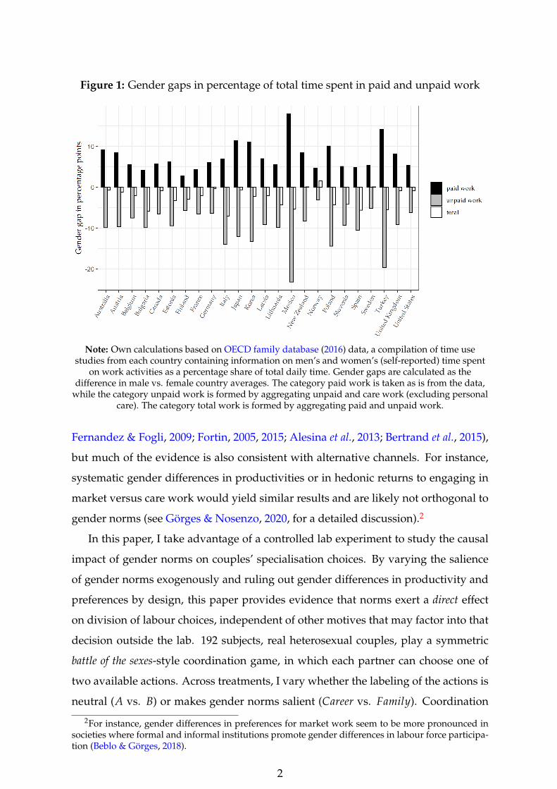
Figure 1: Gender gaps in percentage of total time spent in paid and unpaid work

Note: Own calculations based on OECD family database (2016) data, a compilation of time usestudies from each country containing information on men’s and women’s (self-reported) time spent

on work activities as a percentage share of total daily time. Gender gaps are calculated as thedifference in male vs. female country averages. The category paid work is taken as is from the data,

while the category unpaid work is formed by aggregating unpaid and care work (excluding personalcare). The category total work is formed by aggregating paid and unpaid work.

Fernandez & Fogli, 2009; Fortin, 2005, 2015; Alesina et al., 2013; Bertrand et al., 2015),

but much of the evidence is also consistent with alternative channels. For instance,

systematic gender differences in productivities or in hedonic returns to engaging in

market versus care work would yield similar results and are likely not orthogonal to

gender norms (see Görges & Nosenzo, 2020, for a detailed discussion).2

In this paper, I take advantage of a controlled lab experiment to study the causal

impact of gender norms on couples’ specialisation choices. By varying the salience

of gender norms exogenously and ruling out gender differences in productivity and

preferences by design, this paper provides evidence that norms exert a direct effect

on division of labour choices, independent of other motives that may factor into that

decision outside the lab. 192 subjects, real heterosexual couples, play a symmetric

battle of the sexes-style coordination game, in which each partner can choose one of

two available actions. Across treatments, I vary whether the labeling of the actions is

neutral (A vs. B) or makes gender norms salient (Career vs. Family). Coordination

2For instance, gender differences in preferences for market work seem to be more pronounced insocieties where formal and informal institutions promote gender differences in labour force participa-tion (Beblo & Görges, 2018).

2

occurs when each of the two available actions are simultaneously chosen by one of

the partners (i.e., each partner ‘specialises’ in one of two actions), but payoffs are

asymmetric and favour the player who chose Career/A. Each subject plays with

their real partner and a randomly matched stranger of the same sex as their partner.

The main result of the experiment is that women’s specialisation choices are highly

sensitive to the salience of gender norms. Compared to the Neutral group, women

opt for Career at a significantly lower rate in the Norm group. The reduction is large,

women in Neutral choose Career more than twice as often compared to women in

Norm. Notably, the drop occurs both when women are paired with their partners

and strangers. This shows that gender norms directly affect women’s behaviour

and, by extension, lower their claims to a joint pie, even when they receive no other

forms of compensation and intra-couple redistribution is ruled out (as is the case with

strangers).

A second result is that men’s response to the salience of norms is much weaker

than that of women and sensitive to whether men are paired with a stranger or their

real partner. When paired with their real partner, men in the Norm group are in fact

no more likely to opt for Career than men in Neutral; a quantitatively large, yet sta-

tistically not significant increase of around 20 percentage points is only observed in

stranger pairings. Exploring potential mechanisms for this heterogeneity, I find sug-

gestive evidence that this discrepancy might be a result of men’s marriage market sig-

nalling, in the spirit of Bursztyn et al. (2017). Specifically, I document patterns consis-

tent with the interpretation that some men care to signal progressive gender attitudes

to their potential long-term partners—“acting feminist”—but not to an anonymous,

randomly matched woman. An alternative explanation, differential beliefs regarding

partners’ and strangers’ Career choices, is not borne out by the data.

Apart from its contribution to the growing economics literature on gender norms,

the paper’s perspective on norms as a coordination device relates it to a small num-

ber of experimental studies on the effectiveness of focal points (Isoni et al., 2013, 2014;

Crawford et al., 2008). In a study most closely related to this paper, Holm (2000)

shows that gender in itself can provide a focal point in a symmetric coordination

game where the two pure strategy Nash equilibria result in unequal payoffs. He

presents evidence that mixed-sex pairs of players are indeed more likely to coordi-

nate than same-sex pairs and that the equilibrium that favours the male player is fo-

3

cal. Surprisingly, despite recurring interest in the question of whether gender norms

provide a focal point in the household division of labour problem in the theoreti-

cal literature (Engineer & Welling, 1999; Hadfield, 1999; Baker & Jacobsen, 2007), it

has not been studied empirically. The present paper addresses this gap by study-

ing a classic battle of the sexes game played by real heterosexual couples and mixed-

sex pairs of strangers, thus offering insights into whether societal gender norms, or

couple-specific norms, can improve coordination outcomes.

The paper also contributes to a growing literature on economic experiments with

real couples (for an overview, see Munro, 2018; Hopfensitz & Munro, 2020). Most

closely related to this study are the experiments by Görges (2015) and Cochard et al.

(2018), who study division of labour. Görges (2015) finds that women are more

likely to perform an unpaid real effort task to reach efficiency gains when paired

with their partner compared to women paired with a male stranger. Cochard et al.

(2018) present couples with an abstract public good game and show that women are

no more likely than men to shift money or time from their private into the public

account. This result is somewhat surprising given that, outside the lab, women are

frequently observed to spend more time than men providing the family public good.3

Both Görges (2015) and Cochard et al. (2018) conjecture that their findings may be re-

lated to the salience of gender norms, which is low in the lab setting in Cochard et al.

(2018), and lower for individuals playing with strangers compared to real partners

in Görges (2015). The present paper corroborates this interpretation by providing

first empirical evidence that women tend to claim a smaller share of a joint pie when

gender norms are salient.

The paper is organised as follows: Section 2 lays out the experimental game, while

details on the procedure are provided in Section 3. The main results are supplied in

Section 4, and Section 5 presents analyses regarding the mechanism. Section 6 offers

a discussion and concludes the paper.

2 Experimental design

The present paper examines the effect of gender norms on household specialisation

decisions in a non-cooperative battle of the sexes. The structure of the game is pre-

3This finding by Cochard et al. (2018) is consistent with women’s behaviour in the Neutral groupdiscussed in the present paper, where women and men are equally likely to choose the strategy thatprovides them with a higher payoff, conditional on coordinating.

4

sented in Table 1. Each player of gender g ∈ { f , m} can choose between two actions

a ∈ {A, B} (labeled Career and Family in the Norm group, A and B in the Neutral

group). For a given action chosen by m, f maximises her own pay-off by not match-

ing m’s action and vice versa. Subjects make two one-shot decision, once matched

with their real partner and once with a stranger.4 Payoffs were set at c = 200 ECU and

f = 100 ECU and converted to Euro-cents at a rate of 1:1 at the end of the experiment.5

Table 1: Battle of Sexes, c > f > 0

Player 2

A / Career B / Family

Player 1A / Career 0, 0 c, f

B / Family f , c 0, 0

Note: Strategies were labeled A and B in the Neutral, and Career and Family in the Norm group.

Applying standard game theory, there are two equilibria in pure strategies in this

game: (Career, Family) and (Family, Career). In the neutrally framed version of the

game, the mixed strategy equilibrium involves playing action A (Career) with proba-

bility cc+ f and action B (Family) with f

c+ f , i.e., 23 and 1

3 , respectively, given the payoffs

chosen in the experimental implementation. Expected payoffs are c fc+ f , i.e., nearly 67

ECU, and the probability to coordinate is just below 45%. When gender norms are

salient, i.e. the available actions are labeled Family and Career, coordination rates

might improve according to the focal point effect (Schelling, 1960), which induces ra-

tional players to play the equilibrium that is culturally dominant. In this setting, this

would imply that the ‘traditional’, male-favouring, equilibrium would be reached

more often, thus improving efficiency at the cost of increased inequality to the disad-

vantage of women.

The parameters of the game are chosen such as to capture a stylised decision

problem arising in many families, in which partners have preferences over mone-

tary income and well-raised children. Reflecting the gains from specialisation, total

4While the matrix representation is familiar to economists, the experimental instructions used amore intuitive illustration to convey the decision structure to subjects from different backgrounds.See Appendix A for details.

5A recent meta-study of ultimatum and dictator game studies by Larney et al. (2019) suggests thatbehaviour in strategic interactions is largely invariant to stake size. Given that strategic interaction isat the heart of the present study, the relatively small stake size may be regarded as a minor concern.

5

utility is highest when one partner invests most of their time in children (Family)

and the other in generating income (Career).6 Payoffs are lower (and normalised to

zero), when both spouses invest equally into Career or Family. This does not assume

that the spouse who chooses Family engages in childcare full-time. As is common

in most families today, childcare may be partially outsourced, but the assumption is

that a residual time input must be provided by a parent and reduces the time that

parent can spend on Career.

A second noteworthy feature of the game is that payoffs are asymmetric and

favour the spouse choosing Career. This assumption can be justified in a number

of ways. An intuitive reason is that the spouse who acquires labour earnings may

either have private information about the amount, or some discretionary power over

its distribution, which allows them to determine a split in their favour.7 Another pos-

sibility is that differences in payoffs implicitly reflect future consequences of the ac-

tions, such as a more privileged financial position of the spouse who maintained their

career relative to the caretaker in case of divorce.8 Lastly, and perhaps less gloomy,

the asymmetry in payoffs can simply arise because both spouses care strongly about

their career and prefer spending their time in pursuit of rather than cutting back from

it.

A final important feature of the game is that payoffs are symmetric across the

two equilibria. Thus, total payoffs are equal, regardless of the gender of the player

choosing Career/Family.9 This implies that both genders are equally productive in

each of the two activities, and derive the same utility from engaging in them. Impor-

6Note that these gains do not derive from differences in relative productivities as in Becker (1973),but are inherent to the production function.

7Both phenomena—hiding of income or windfalls from spouses and exercising control over in-dividually obtained income—are well-documented in the experimental family economics literature(Ashraf, 2009; Iversen et al., 2011; Mani, 2011; Castilla & Walker, 2013; Kebede et al., 2013; Ambler,2015; Hoel, 2015).

8Once children have left the household, both parents derive the same utility from them, regardlessof parents’ marital state. Both spouses will now invest all their time in market work, but levels ofwage productivity have diverged because one spouse has been (more) absent from the labour marketin period 1. This may create an incentive for the richer spouse to divorce the poorer one, if in doing sothey can keep a larger share of their labour income to themselves.

9Given that much of the recent debate in economics is concerned with the potentially detrimentaleffects to household efficiency, higher total payoffs in the female-favouring equilibrium would havealso presented an interesting case to examine. Predictions would clearly be different for the Neutralcase, since the expected rate of reaching the female-favouring equilibrium would be higher in thispayoff structure. Yet, predictions for the effect of norms would be qualitatively similar, as we wouldexpect their salience to raise the relative likelihood of the male-favouring equilibriumin the Normgroup.

6

tantly, payoffs are constant across treatments, allowing us to investigate the impact

of the salience of gender norms on choices independent of other considerations. This

is important since it is often argued that couples’ specialisation choices likely reflect

that women, relative to men, prefer time with children over time in the labour mar-

ket or are more productive in child-rearing. Outside the lab, it is hard to determine

the extent to which such gender differences exist and matter. Moreover, it is virtu-

ally impossible to separate them from the effect of societal norms, as they are likely

correlated. For instance, prior research has documented lower relative preferences

for work in women (Beblo & Görges, 2018) and stronger beliefs about higher relative

returns of maternal time inputs on child outcomes (Bauernschuster & Rainer, 2012;

Fortin, 2015) in societies with more traditional gender norms.

Analysing the household specialisation problem as a non-cooperative, one-shot

battle of the sexes game is of course a gross simplification of the reality of this decision.

Yet, it allows us to capture the essence of a specific decision environment in which

we want to study the influence of gender norms. A one-shot simultaneous move

game without communication provides the desired properties of a non-cooperative

bargaining environment.10 It is important to note that I create this non-cooperative

environment intentionally for all subjects to be observed in, regardless of whether

they would usually come to an agreement using cooperative bargaining. One rea-

son for this is rather technical. Communication would have changed the decision

environment into a cooperative one for some couples (those couples who generally

bargain cooperatively), whereas it would have remained a non-cooperative choice

for others. While this would have complicated the comparison between Neutral and

Norm in real couples considerably, comparisons between real couples and anony-

mous strangers would have been rendered meaningless entirely. Strangers would

have likely continued to bargain non-cooperatively, given the lack of possibilities to

make binding agreements, even with communication.

There are also important conceptual reasons for studying specialisation choices

as a non-cooperative bargaining game. While family economic models often as-

sume cooperation among household members and thus predict productive efficiency

(Manser & Brown, 1980; McElroy & Horney, 1981; Chiappori, 1988), often non-cooperative

10Communication was prevented using several measures. Partners were seated in closed booths,several booths apart from each other. They had to turn over their mobile phones to the lab team forthe duration of the experiment. See Section 3 for details.

7

behaviour plays an important role, at least in the threat point (Lundberg & Pollak,

1994; Konrad & Lommerud, 2000). Empirically, numerous economic experiments

with couples have documented that non-cooperative behaviour is far from uncom-

mon (Peters et al., 2004; Ashraf, 2009; Iversen et al., 2011; Mani, 2011; Castilla &

Walker, 2013; Kebede et al., 2013; Ashraf et al., 2014; Cochard et al., 2014; Ambler, 2015;

Beblo et al., 2015; Hoel, 2015; Beblo & Beninger, 2017). Closely related to the special-

isation game studied here, Fahn et al. (2016) have shown that divorce and alimony

legislation affects whether couples bargain cooperatively or non-cooperatively and

that non-cooperative environments lead to inefficiently low public good investments

with lower fertility. In light of rising divorce rates and weakened alimony laws in

many countries (e.g., for the US, see Stevenson & Wolfers, 2007), relationships are

increasingly characterised by contractual incompleteness and thus non-cooperation.

While bargaining over the division of labour is plausibly a repeated game, there

are good reasons to focus on the one-shot version of the game when studying the

effect of norms on outcomes. It is likely that the outcome of the ‘first shot’ is strongly

predictive of outcomes in subsequent games and is therefore the most relevant to

study. The reason is that specialisation choices typically feed back into spouses’ rela-

tive productivities, since wage profiles diverge as one partner focuses more on their

career than the other. As a result, the spouse who assumed the primary caregiver

role upon arrival of the first child will likely do so upon arrival of the second.11 The

recent COVID-19 pandemic attest to this: As schools and childcare facilities closed,

households’ demand for private child care is most likely met by the parent who had

already supplied more childcare before the pandemic, in most couples the mother

(Fuchs-Schündeln et al., 2020). Moreover, recent survey evidence shows that a size-

able fraction of couples have never discussed their division of household and market

work during lockdown (Cosaert et al., 2021), when excess childcare burdens were at

their peak, indicating that the bargaining over the division of this burden followed

indeed a non-cooperative protocol not entirely unlike the one we study here using a

stylized battle of the sexes game.

In light of these considerations, the aim of the present paper is to test empirically

whether gender norms affect the probability that couples reach a male- vs. female

11This means that the payoff structure of the game would change such that the equilibrium in whichspouses choose the same actions as in a past game now generates higher individual and total payoffsthan before, thus increasing the likelihood that spouses coordinate on it.

8

favouring division of labour in a non-cooperative setting. Since a higher rate of male-

favouring equilibra comes at the cost of female players, it is important to understand,

in a scenario where economic advantages or gains in non-monetary satisfaction from

time spent with children can be ruled out, whether such a shift can occur simply

due to the salience of gender norms. Comparing differences in outcomes between

Norm and Neutral across pairs consisting of real partners and strangers allows us to

further assess whether inequality between men and women only arises when it can

easily be attenuated by intra-couple redistribution (as is the case for real partners) or

whether subjects are similarly likely to expect that women accept a smaller share of

the pie when that division is final (as is the case with strangers). In addition, com-

paring coordination rates across real partners and strangers might reveal whether

individual norms can superimpose societal norms. For example, individuals holding

progressive gender attitudes might play the female-favouring equilibrium with their

partners but rationally expect a randomly drawn stranger from a representative dis-

tribution of gender attitudes to play differently, implying that the female-favouring

equilibrium occurs with a higher frequency in real couples compared to strangers.12

3 Procedure & sample

The experiment was programmed in ztree (Fischbacher, 2007) and conducted in the

economics lab at the University of Hamburg in 2016 and 2017. The battle of the sexes

game analysed in this paper was part of a larger experiment on labour division, anal-

ysed in a companion paper (Görges, 2019), and was added at the end of 9 out of 12

sessions. Completing this part took about 10 minutes in sessions lasting 2.5 hours on

average. Average payouts for the sessions as a whole were e27.43 (approximately

$34 at the time of writing this paper). Four sessions (80 participants) were assigned

to the Norm, and the remaining five (112 participants) to the Neutral group. All sub-

jects played the game with both their real partner and a randomly matched stranger,

12The reverse phenomenon might, of course, occur when subjects expect that gender attitudes inthe student population are on average more progressive than their own. Moreover, if subjects areinequality-averse, they may prefer an equal payoff of 0 over an unequal distribution, and thus tryto prevent coordination. But since advantageous and disadvantageous inequality aversion wouldhave to be rather pronounced to alter the pure-strategy equilibria (2 and 1 for advantageous anddisadvantageous inequality aversion, respectively, in a Fehr & Schmidt (1999) model given the payoffschosen in this experiment), I do not consider it as a motive. Moreover, Charness & Rabin (2002) haveshown in their large-scale experiments that the majority of individuals are most strongly concernedwith raising social welfare, more so than inequality.

9

where partner gender was held constant across pairings.13 Thus, the data features

between-subject variation in the presence of a gender norm focal point and within-

subject variation in the pairing.

Subjects were recruited via hroot (Bock et al., 2014) from a regular student subject

pool. The invitation email instructed subjects to pre-register their partner and bring

them to the experimental session. Being married or cohabitating with their partner

was not required, nor were partners required to be enrolled as students. Upon ar-

rival in the lab, participants were reminded that they needed to be true couples in a

relationship, not merely study partners or housemates, in order to participate in the

experiment. They were asked to leave if this was not the case; however, no one left

the experiment. Additional ex-post checks that mitigate concerns regarding potential

“fake couples” are provided in Appendix B.

Instructions for the game explicated the payoff consequences of the two available

actions for both possible scenarios (partner choosing A/Career or B/Family). They

further informed subjects that they would play once with their partner and once with

a randomly matched stranger (same sex as partner), and that they would have no

knowledge of their partner’s chosen action when making their decision, but would

find out about each other’s respective choices once the payouts were revealed.14 As

the experiment involved only a simple choice between two options, subject’s com-

prehension was not tested formally, but subjects were invited to raise their questions

in case of comprehension issues.

After having read the instructions, subjects were paired with their first partner

(real or stranger) and entered their choice. Next, they were asked to predict their part-

ner’s decision. Upon completing this step, but before finding out the result, they were

paired with their second partner (real or stranger) to repeat the previous steps. Once

completed, subjects were confronted with four more prediction tasks: How many

women (men) had chosen Career when playing with their real partner (stranger)?

All prediction tasks were incentivised.15 Finally, the outcomes of both games and the

13Order effects were ruled out by design because the result of each interaction was not revealed untilboth had been completed. Based on a regression of round-specific earnings on a round-2 dummy, wecannot reject the hypothesis that the difference between round 1 and 2 earnings is zero (p = .36). Forcompleteness, Appendix-Table C.5 shows that the main results presented in this paper are robust toincluding the round-2 dummy as control.

14A translated version of the instructions can be found in Appendix A.15Throughout the experiment, subjects were asked to make several predictions and were informed

that two-thirds of the predictions would be randomly selected and paid out. They received 50ECU

10

corresponding payoffs were revealed.

Descriptive statistics are reported in Table 2.16 All sessions were gender balanced

by design. On average, participants in the Neutral group were about 25 years old,

and 27 years old in the Norm group. Because the difference is significant, age will

be included as a control in subsequent analyses. Union characteristics are measures

that describe subjects’ relationships with their partner. Most were very similar across

treatments: The average union duration (time spent in the relationship with their

partner) was three years, almost a third of the couples were cohabiting, and partici-

pants reported high satisfaction levels with their relationship on average. The Norm

and Neutral groups differ with respect to the proportion of married couples: 7% of

the participants in the Neutral group were married, while no couples in Norm were

married. Consequently, marital status will also be included as a control variable in

subsequent analyses.

Most subjects were currently enrolled in some form of educational institution,

primarily university. The Norm and Neutral samples do not differ statistically with

respect to enrollment status or the level of study. Furthermore, the two groups are

very similar with respect to labour market activity. About a third of subjects are not

active at all, and the rest are either unemployed or employed (full-time, part-time, or

irregularly). Finally, the samples differ with respect to the proportion of subjects who

ever participated in a lab experiment; thus, this indicator variable will be included in

the subsequent analyses as well.17

4 Main results

4.1 Do gender norms affect coordination outcomes?

We begin by examining the effect of the salience of gender norms on coordination

outcomes. Figure 2 summarises the raw data, breaking down by treatment (Norm vs.

Neutral) the fraction of pairings—strangers (real partners) in the left (right) panel—

for correctly predicting their partners’ choice between Career vs. Family, and 100ECU for the totalnumber of men (women) choosing Career in their session.

16The data analyses and the presentation of results in this paper were prepared using the R pro-gramming environment for statistical computing (R Core Team, 2018), version 3.6.3, and several add-onpackages: emmeans (Lenth, 2020), extrafont (Chang, 2014), glue (Hester, 2020), lme4 (Bates et al., 2015),MASS and nnet (Venables & Ripley, 2002), readxl (Wickham & Bryan, 2019), stargazer (Hlavac, 2018),texreg (Leifeld, 2013), tidyverse (Wickham et al., 2019), and xfun (Xie, 2020).

17Appendix-Table C.5 presents several robustness checks, including results from a restricted sampleof subjects who never participated in an experiment. The results are qualitatively similar, but lackstatistical power as the sample is reduced by more than half.

11

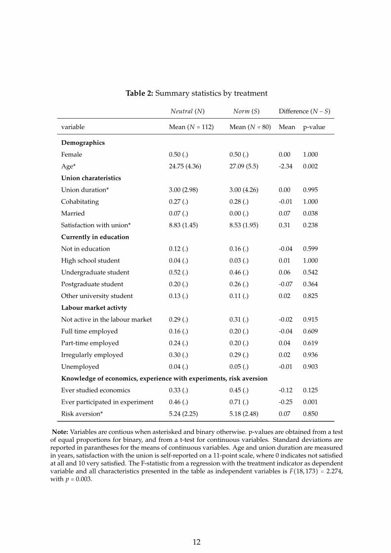
Table 2: Summary statistics by treatment

Neutral (N) Norm (S) Difference (N − S)

variable Mean (N = 112) Mean (N = 80) Mean p-value

Demographics

Female 0.50 (.) 0.50 (.) 0.00 1.000

Age* 24.75 (4.36) 27.09 (5.5) -2.34 0.002

Union charateristics

Union duration* 3.00 (2.98) 3.00 (4.26) 0.00 0.995

Cohabitating 0.27 (.) 0.28 (.) -0.01 1.000

Married 0.07 (.) 0.00 (.) 0.07 0.038

Satisfaction with union* 8.83 (1.45) 8.53 (1.95) 0.31 0.238

Currently in education

Not in education 0.12 (.) 0.16 (.) -0.04 0.599

High school student 0.04 (.) 0.03 (.) 0.01 1.000

Undergraduate student 0.52 (.) 0.46 (.) 0.06 0.542

Postgraduate student 0.20 (.) 0.26 (.) -0.07 0.364

Other university student 0.13 (.) 0.11 (.) 0.02 0.825

Labour market activty

Not active in the labour market 0.29 (.) 0.31 (.) -0.02 0.915

Full time employed 0.16 (.) 0.20 (.) -0.04 0.609

Part-time employed 0.24 (.) 0.20 (.) 0.04 0.619

Irregularly employed 0.30 (.) 0.29 (.) 0.02 0.936

Unemployed 0.04 (.) 0.05 (.) -0.01 0.903

Knowledge of economics, experience with experiments, risk aversion

Ever studied economics 0.33 (.) 0.45 (.) -0.12 0.125

Ever participated in experiment 0.46 (.) 0.71 (.) -0.25 0.001

Risk aversion* 5.24 (2.25) 5.18 (2.48) 0.07 0.850

Note: Variables are contious when asterisked and binary otherwise. p-values are obtained from a testof equal proportions for binary, and from a t-test for continuous variables. Standard deviations arereported in parantheses for the means of continuous variables. Age and union duration are measuredin years, satisfaction with the union is self-reported on a 11-point scale, where 0 indicates not satisfiedat all and 10 very satisfied. The F-statistic from a regression with the treatment indicator as dependentvariable and all characteristics presented in the table as independent variables is F(18, 173) = 2.274,with p = 0.003.

12

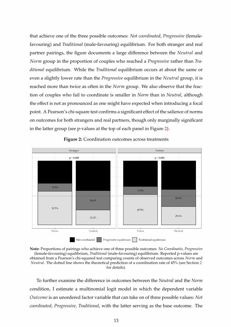
that achieve one of the three possible outcomes: Not coordinated, Progressive (female-

favouring) and Traditional (male-favouring) equilibrium. For both stranger and real

partner pairings, the figure documents a large difference between the Neutral and

Norm group in the proportion of couples who reached a Progressive rather than Tra-

ditional equilibrium. While the Traditional equilibrium occurs at about the same or

even a slightly lower rate than the Progressive equilibrium in the Neutral group, it is

reached more than twice as often in the Norm group. We also observe that the frac-

tion of couples who fail to coordinate is smaller in Norm than in Neutral, although

the effect is not as pronounced as one might have expected when introducing a focal

point. A Pearson’s chi-square test confirms a significant effect of the salience of norms

on outcomes for both strangers and real partners, though only marginally significant

in the latter group (see p-values at the top of each panel in Figure 2).

Figure 2: Coordination outcomes across treatments

Note: Proportions of pairings who achieve one of three possible outcomes: No Coordinatio, Progressive(female-favouring) equilibrium, Traditional (male-favouring) equilibrium. Reported p-values are

obtained from a Pearson’s chi-squared test comparing counts of observed outcomes across Norm andNeutral. The dotted line shows the theoretical prediction of a coordination rate of 45% (see Section 2

for details).

To further examine the difference in outcomes between the Neutral and the Norm

condition, I estimate a multinomial logit model in which the dependent variable

Outcome is an unordered factor variable that can take on of three possible values: Not

coordinated, Progressive, Traditional, with the latter serving as the base outcome. The

13

main variables of interest are the treatment indicators: Norm (1 if an outcome was

observed in the Norm group and 0 otherwise), Partner (1 for outcomes that occured

between real partners and 0 otherwise), and their interaction. Since outcomes occur at

the couple level rather than the individual level, I use women only for the estimation

to ensure that the sample is not artificially inflated; the results are (nearly) identical

when using the male sample.18 Since each woman plays once with their partner and

once with a randomly matched stranger, the estimation is based on N = 196 observa-

tions. To account for potentially heterogeneous treatment effects, estimated standard

errors are Huber-White robust.

Table 3 reports the estimated coefficients of interest from the model alongside the

estimated average marginal effect of the Norm treatment on the probability to reach

any of the three outcomes. The results in column (1) stem from a model without any

additional covariates. In column (2), I include controls for age, duration of the union,

a survey measure for risk aversion,19 as well as indicators for (i) being married to

one’s partner, (ii) having ever studied economics, and (iii) having ever participated

in a lab experiment. As can be seen by comparing columns (1) and (2), controling

for additional covariates hardly changes the results on the coefficients of interest.

The interpretation of the negative sign of the coefficients is as follows: Playing in

Norm rather than Neutral significantly decreases the probability to reach the Progres-

sive equilibrium relative to the Traditional equilibrium, the base outcome. Similarly,

the probability of miscoordinating rather than reaching the Traditional equilibrium

also increases significantly in the Norm treatment.

Since the effect of playing with one’s Partner rather than with a stranger, as well

as the interaction between the treatment indicators Norm × Partner are statistically

insignificant, the table presents the average marginal effect of playing in the Norm

rather than the Neutral group on the probability to reach either of the three outcomes.

Overall, the estimated marginal effects of the treatment from the full model are re-

markably similar to the treatment differences in the raw data shown in Figure 2. As

can be seen in the rows labelled AME Norm in Table 3, the probability to to reach a

Progressive equilibrium declines by around 17 percentage points, whereas the proba-

18Slight differences in estimated coefficients are due to the inclusion of individual-level controls thatmay differ between partners, such as risk aversion, whether the subject ever studied economics or hasever participated in an experiment before.

19The questionnaire item was validated by Dohmen et al. (2011).

14

Table 3: Estimated treatment effects on coordination outcomes (multinomial logit)

Outcome (1) (2)

Progressive

Norm -1.703∗∗∗(0.62) -1.805∗∗∗(0.69)

Partner -0.333 (0.52) -0.334 (0.52)

Norm × Partner 0.433 (0.88) 0.434 (0.88)

AME Norm -0.161∗∗ (2.84) -0.171∗∗∗(0.06)

Traditional(Reference)

Norm — —

Partner — —

Norm × Partner — —

AME Norm 0.241∗∗∗ (3.46) 0.255∗∗∗ (0.075)

Not coordinated

Norm -1.099∗∗ (0.49) -1.155∗∗ (0.51)

Partner -0.247 (0.47) -0.248 (0.47)

Norm × Partner 0.480 (0.67) 0.484 (0.68)

AME Norm -0.080 (1.12) -0.085 (0.08)

Controls No Yes

N 192 192

Note: Coefficients from a multinomial logistic regression of Coordination Outcome on treatment in-dicators (Norm, Partner), with Traditional equilibrium as reference category. Rows labeled AME Normshow the average marginal effects of the Norm treatment on the probability to reach a given outcome.Column (1) shows results from a model only including treatment indicators, column (2) shows resultswith additional controls for subject Age, Riskaversion, Unionduration, Cohabiting, Married, Everinlab,Everstudiedecon. Estimations are based on the female sample. Huber-White robust standard errors arereported in parantheses, stars indicate significance at ∗p<0.1; ∗∗p<0.05; ∗∗∗p<0.01.

bility reach a Traditional equilibrium increases by around 25 percentage points for a

couple in Norm relative to one in Neutral. Both effects are statistically significant at

the 1-percent level. As expected in the presence of the focal point that norms pro-

vide, miscoordination rates also decline in the Norm condition, by nearly 9 percent-

age points, but the effect fails to reach statistical significance at conventional levels

(p = .29 in the model with controls).

Given the payoff structure of the game–higher payoffs for the male (female) part-

ner in the Traditional (Progressive) equilibrium–the differences in coordination out-

comes across treatments have direct consequences for payoff inequality. Since the

Traditional equilibrium is the most frequent outcome in the Norm group, the male-

15

female earnings gap in this group is large and positive; on average, women earn 67%

of men’s income. By contrast, both genders earn about the same in the Neutral group:

around 70% of the average male income in the Norm group, reflecting the somewhat

higher rate of coordination failure in this group. Average earnings by gender and

treatment are summarised in Appendix-Table C.2.

Why is it that the salience of norms has a strong effect on the type of equilibrium

couples coordinate on, but surprisingly little effect on the overall coordination rate?

To better understand this result, a closer look at subjects’ individual Career choices is

warranted.

4.2 Do gender norms affect individual Career choices?

Next, we investigate the effect of gender norms on subjects’ choices. A priori, one

might expect that both men and women adapt their behaviour in the presence of a

gender norm focal point, albeit in opposite directions (i.e., compared to the Neutral

group, women choose Career less frequently in Norm, while men choose it more of-

ten). To test these hypotheses, I estimate a linear probability model in which the

dependent variable is an indicator, Career, which is equal to one if an individual

chose option A/Career and zero otherwise. The key explanatory variables of interest

are indicators for playing in the Norm treatment, with one’s real Partner, for being

of Female gender and their respective interactions. To address potential clustering of

observations at the session level, I estimate a multi-level model that includes session-

specific random intercepts (Moffatt, 2015) and Huber-White robust standard errors

to account for possible heterogeneity in treatment effects.20

The regression results are provided in Table 4. Column (1) includes indicators

for the Norm group, female subjects, and their interactions. The coefficient on the

intercept thus gives the proportion of male subjects choosing Career in the Neutral

group (53.6%). The coefficient on Norm tells us that this share increases slightly (by

about 9 percentage points) in the Norm group, but the difference is not statistically

significant. Looking at the coefficient on Female, we learn that, in the Neutral group,

women’s propensity to choose Career does not differ from that of men. However, the

20Since the treatment variable Norm varies at the session level, its effect cannot be identified usinga session-fixed effects model. Reassuringly though, all interaction effects with the Norm indicator thatare studied in this paper, such as Female, Partner and Committed (see Section 5.2) turn out very similarin a fixed-effects model compared to those presented in the paper obtained from the multilevel model.Results are available upon request.

16

Table 4: Treatment effects on Career choices

(1) (2) (3)

Norm 0.089 (0.11) 0.217 (0.16) 0.192 (0.17)

Female 0.027 (0.02) 0.071 (0.08) 0.068 (0.08)

Norm x Female -0.402***(0.12) -0.471**(0.22) -0.467**(0.22)

Partner 0.107***(0.04) 0.107***(0.04)

Norm x Partner -0.257**(0.12) -0.257**(0.12)

Female x Partner -0.089 (0.14) -0.089 (0.14)

Female x Norm x Partner 0.139 (0.23) 0.139 (0.23)

Intercept 0.536*** (0.04) 0.482***(0.04) 0.423** (0.17)

N 384 384 384

Controls No No YesNote: Results obtained from a multilevel linear model including session-level random intercepts to

account for clustering. Huber-White robust standard errors are reported in parantheses; starsindicate significance ∗p<0.1; ∗∗p<0.05; ∗∗∗p<0.01. The full set of controls includes: Age,

Unionduration, Married, Riskaversion, Everstudiedecon, Everinlab. Estimated group means from thefull specification (3) are shown in Figure 3.

large and statistically significant coefficient on the interaction, Norm × Female shows

that the effect of gender norm salience on women’s Career choices differs markedly

from the effect on men’s choices, with the difference in differences amounting to 40

percentage points. Taken together with the coefficient on Norms, this indicates that

women’s propensity to choose Career decreases by more than 30 percentage points

in Norm relative to Neutral. In sum, these results suggest that women respond to the

salience of gender norms while men do not, despite the economic incentives for both

genders to do so if norms make the Traditional equilibrium focal. This is surprising

and calls for further investigation.

Column (2) of Table 4 generates the group means disaggregated by familiarity

with the partner, and Column (3) presents the results additionally controlling for the

familiar set of personal covariates. To ease interpretation, predicted group means

obtained from estimation (3), holding personal covariates fixed at their average, are

plotted in Figure 3. It also displays p-values obtained from testing for differences

in group means using F-tests of (linear combinations of) coefficients. The left (right)

panel shows the predicted means for women (men). Within each panel, the first

(second) set of bars refers to pairings with the real partner (stranger). Dark (light)

17

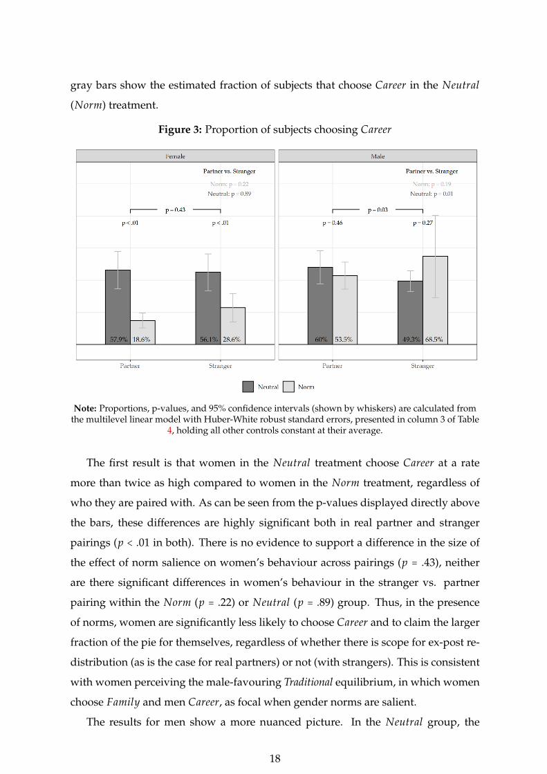
gray bars show the estimated fraction of subjects that choose Career in the Neutral

(Norm) treatment.

Figure 3: Proportion of subjects choosing Career

Note: Proportions, p-values, and 95% confidence intervals (shown by whiskers) are calculated fromthe multilevel linear model with Huber-White robust standard errors, presented in column 3 of Table

4, holding all other controls constant at their average.

The first result is that women in the Neutral treatment choose Career at a rate

more than twice as high compared to women in the Norm treatment, regardless of

who they are paired with. As can be seen from the p-values displayed directly above

the bars, these differences are highly significant both in real partner and stranger

pairings (p < .01 in both). There is no evidence to support a difference in the size of

the effect of norm salience on women’s behaviour across pairings (p = .43), neither

are there significant differences in women’s behaviour in the stranger vs. partner

pairing within the Norm (p = .22) or Neutral (p = .89) group. Thus, in the presence

of norms, women are significantly less likely to choose Career and to claim the larger

fraction of the pie for themselves, regardless of whether there is scope for ex-post re-

distribution (as is the case for real partners) or not (with strangers). This is consistent

with women perceiving the male-favouring Traditional equilibrium, in which women

choose Family and men Career, as focal when gender norms are salient.

The results for men show a more nuanced picture. In the Neutral group, the

18

rates of choosing Career are around 50-60%, similar to the rates in women.21 Perhaps

surprisingly, Figure 3 confirms that there is no impact of gender norms on men’s

behaviour when paired with their partner (p = .46). The expected increase in Career

choices in the Norm treatment is only observed in stranger pairings, where we see

a quantitatively large difference of almost 20 percentage points, yet not significant

statistically at conventional levels (p = .27). The difference-in-difference in the effect

of norms across partner and stranger pairings, however, is significant statistically at

the 5-% level (p = .03). Thus, it appears that there is at best weak evidence for an effect

of gender norms on men’s Career choices, and a suprising heterogeneity in men’s

responses across partner and stranger pairings. The following Section 5 presents an

exploration of potential mechanisms.

5 Mechanisms

The main results presented in Section 4 have shown that women’s Career choices

change across treatments in a way that is consistent with the presence vs. absence of

a gender norm focal point, i.e. their rate of choosing Career decreases when norms

are salient. Men’s response, however, responds much less to the salience of norms

and is heterogeneous across partner and stranger pairings. One explanation could be

related to differential beliefs regarding their partners’ choice. If men expect their real

partners to hold more progressive attitudes than the average female student, they

may consider them more likely to choose Career. While the following subsection 5.1

shows that this explanation is not borne out by the data, subsection 5.2 investigates

a marriage market motive in the spirit of Bursztyn et al. (2017): Men may want to

signal progressive gender attitudes, a quality that might be desirable in the marriage

market.

5.1 Differences in beliefs regarding real partner’s and stranger’s choices?

If beliefs were to explain Career choices across treatments, women’s beliefs about

men’s behaviour (real partners and strangers) ought to show higher rates of Career

choices in the Norm than in the Neutral group. Men’s beliefs regarding women’s

choices, however, should not differ much between Norm and Neutral, but should

show the lowest levels of Career choices for the randomly matched women in the

21Differences between men and women are never (always) significant in the Neutral (Norm) treat-ment.

19

Norm group. As detailed in Appendix A, participants of both genders were incen-

tivised to provide their best guess of a) what their real partner chose; b) what their

randomly matched stranger chose; c) how many men in their session chose Career

when paired with their real partner; d) how many men chose Career when paired

with a stranger; e-f) as c-d) but about women.

For the analyses presented in this subsection, I use these predictions to calculate

(i) the proportion of subjects who predicted that their partner chose Career, and (ii)

subjects’ predicted proportion of men (women) in their session who chose Career.22

Comparing beliefs about the partner subjects are matched with to beliefs about others

in the session serves two main purposes. First, in the case of strangers, subjects’ be-

liefs about a randomly matched stranger and beliefs about the average behaviour of

strangers in their session should be identical; the comparison of these two measures

can thus attests to the quality of the data if results are, in fact, similar. Second, a com-

parison of beliefs about one’s real partner and the average behaviour of individuals

paired with their partner in the session could provide additional clues as to whether

men’s own Career choices might in part be explained by men thinking of their own

partners as very different (more progressive) than the average woman paired with

their partner.23

The empirical strategy used to analyse beliefs is very similar to the one used in

the previous Section 4, i.e. I estimate linear multilevel models accounting for session-

specific clustering to gauge the effects of the treatment indicators Norm, Female,

Partner and their interactions. Estimated standard errors are Huber-White robust.

Figure 4 summarises the results; the corresponding regression results are shown in

Appendix-Table C.3. Men’s beliefs about women are displayed in the panels in the

first column, women’s beliefs about men in the second column. The top two panels

display the proportion of subjects thought to have chosen Career by their partner, the

bottom two show average beliefs about the proportions of subjects in their session

who chose Career. The figure is structured in the same manner as the previous one,

22Predicted proportions are obtained by dividing the absolute number of men (women) that thesubject predicted to have chosen Career by the total number of male (female) players in their session.Note that, although subjects of both genders were asked to predict the number of men and womenin their session, I only use cross-gender predictions, i.e. women’s (men’s) predictions about men(women), as those are the ones relevant for the strategic decision.

23In addition, Appendix-Section C.2 further explores the accuracy of beliefs and shows that bothmen’s and women’s beliefs are actually most likely to be accurate when they play in the Norm treat-ment and are asked to predict their real partner’s choice.

20

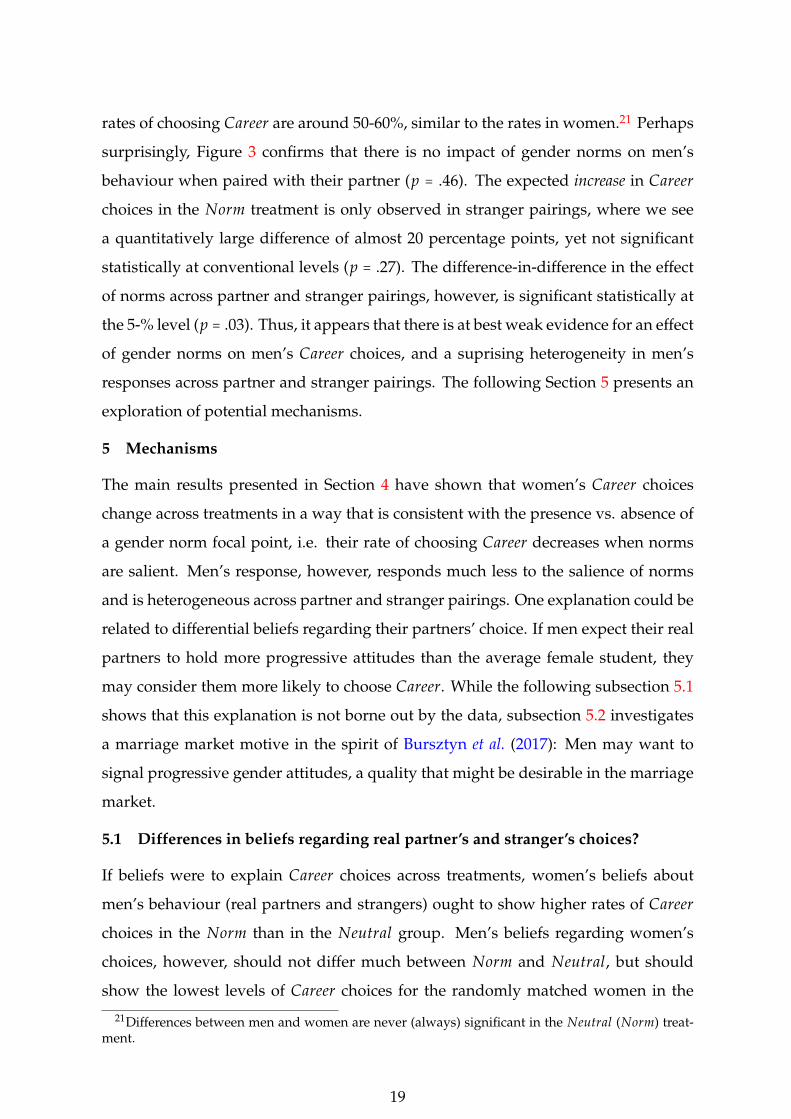
with dark (light) gray bars displaying the averages in the Neutral (Norm) treatment

and the first (second) groups of bars in each panel referring to partner (stranger) pair-

ings. In addition, black dots indicate the actual Career choice rates of the group for

whom beliefs are elicited, i.e. women’s actual choices are displayed together with

men’s beliefs about women’s choices and vice versa.24

Figure 4: Beliefs about Career choices across treatments

Note: Proportions, p-values, and 95% confidence intervals (shown by whiskers) are calculated from amultilevel linear model with Huber-White robust standard errors, presented in column 3 of

Appendix-Table C.3, holding all other controls constant at their average. Black dots show actualbehaviour in the group for which beliefs are displayed (as reported in Figure 3).

Looking at men’s beliefs, we see no evidence that men anticipate different re-

sponses in terms of women’s Career choices in Neutral vs. Norms. Neither when

asked about all women in the session, nor about the partner they are paired with, do

24Actual choices of course do not differ across rows (i.e., women’s actual rate of choosing Careerwhen paired with their partner in the Neutral treatment is the same, regardless of whether we look atmen’s beliefs about all women in the session who played with their partner or at men’s beliefs aboutthe choices of their female partners).

21

men’s predictions about women’s Career choices differ between Neutral and Norm.

As a result, men greatly overestimate women’s rate of choosing Career in the Norm

group. While at first glance this pattern is consistent with men’s lack of response

in their own Career choices across treatments, it cannot explain the observed hetero-

geneity in men’s response to the salience of norms when paired with their real partner

vs. a stranger. Specifically, wee see no evidence supporting the hypothesis that men

expect their real partners to hold more progressive attitudes than a random female

stranger, which would imply men expect higher Career rates among the women who

are their partners. By contrast, we see that the rate of men in the Norm treatment

who expect their partner to choose Career is significantly lower than that of the same

men asked about the choice of their randomly matched stranger (33 vs. 66 percent,

p = .01). A similar pattern can be seen in men’s beliefs about all women in the ses-

sion, which indicates men expect women playing with strangers to be more likely to

choose Career than women playing with their partners.25

Women’s beliefs appear more consistent with their own Career choices, which

decrease significantly when gender norms are salient, they predict higher rates of

Career in men’s choices in the Norm than in the Neutral group. However, these dif-

ferences are only statistically significant in women’s beliefs about all men in their

session (p = .01 for beliefs about men playing with partners, p < .01 strangers).26

Women’s beliefs about the partner they are matched with show a similar pattern, but

no statistical significance (p = .11 and p = .56 for real partners and strangers, respec-

tively). Note however, that confidence intervals are larger for the means obtained

from the regression using the binary outcome variable (beliefs about Career choice of

partner) compared to the continuous outcome (beliefs about proportion of subjects

choosing Career).

Taken together, the evidence indicates that beliefs seem to explain Career choices

for women, but do not resolve the puzzle of men’s differential response to the salience

of gender norms depending on whether they play with a stranger or their real part-

ner. In sum, these results provide no evidence that men react more strongly to the

25Given that the difference between men’s beliefs about women playing with their partners vs.playing with strangers is significant at the 1-percent level in both Norm and Neutral group, it mightreflect a more general belief about women playing more hawkish when matched with a stranger asopposed to their partners.

26Here, the predicted rates of men choosing Career are also substantially higher than the true rates,except for men playing with their real partner in Neutral.

22

presence of gender norms when paired with a stranger compared to when paired

with their partner because men believe that their real partners are likely to behave

more progressively.

5.2 Men ‘acting feminist’?

An alternative explanation for the heterogeneity in men’s response to the salience

of norms across partner and stranger pairings could be a marriage market motive.

This subsection explores the possibility that men’s behaviour may reflect signalling

of progressive gender attitudes. The basic idea follows Bursztyn et al. (2017) and

builds on the assumptions that a) men and women want to be successful in the mar-

riage market, i.e. secure a long-term partner, b) women tend to value progressive

gender attitudes in men, which is supported by several studies for the US (Pedulla &

Thébaud, 2015), UK (Auspurg et al., 2017) and Germany (Lück, 2015),27 and c) men

are aware of this and signal progressive attitudes when obsorved by a potential mate,

’acting feminist’.

Based on these assumptions, incentives and opportunity for men to signal pro-

gressiveness may arise in the Norm treatment. Given that women in Norm choose

Career at lower rates compared to Neutral, men would maximise their income by

choosing Career at higher rates. Yet, signalling progressiveness at the cost of lower

expected earnings in the game could be rational for some men, whose relationship is

not yet committed. As opposed to men who are already in committed relationships,

men in non-committed relationships still compete for their partner in the marriage

market and may thus benefit from signalling progressiveness. This may create an in-

centive for non-committed men to behave differently towards their real partner than

towards a stranger, since they only care about their signal to the former, but not how

their actions are perceived by a random female stranger.28 Men who are in commit-

ted relationships should not act differently when their behaviour is observed by their

real partner versus a stranger.

To test this hypothesis, I follow Bursztyn et al. (2017) in defining a relationship

as committed when partners cohabitate, using information on participants’ cohabita-

27The studies indicate that particularly college educated women, like the ones participating in thepresent study, tend to value more progressive gender attitudes and division of labour arrangements.

28Choosing Family instead of Career in a lab game with relatively low stakes is a particularly easyand cheap way for men to signal progressive gender attitudes. Whether or not women actually findthis credible is a question the present study cannot answer.

23

tion status from the post-experimental questionnaire. I estimate separate regressions

for male and female subjects, using an otherwise similar model specification as in

the preceding sections. That is, I estimate multi-level linear probability models and

Huber-White robust standard errors. The indicator for choosing Career serves as the

dependent variable and indicators for Norm, Partner, Committed and their interac-

tions as main explanatory variables of interest. The usual set of controls are included

alongside a control for beliefs about the relevant partner’s choices examined in the

previous subsection.

Figure 5 plots the predicted means obtained from the full models, holding other

covariates fixed at their means (see Appendix-Table C.4 for the estimated coefficients

of the models). Similar to the Figures in the preceeding sections, Figure 5 reports the

share of subjects who chose Career, but separately for individuals in non-committed

(committed) relationships in the top (bottom) panels. Differences in means across

groups are tested for statistical significance using F-tests of (linear combinations of)

coefficients from the full regression model; the resulting p-values are shown in the

graph.

For the reasons outlined above, we suspect that men in non-committed relation-

ships might stand to gain from signalling in the Norm treatment. Our primary inter-

est therefor rests on men in non-committed relationships and the difference in their

rate of choosing Career when playing with their real partner versus a stranger. Con-

sistent with the signalling hypothesis, we see that Career rates of non-committed men

paired with their partner are actually lower in Norm than in Neutral (33% vs. 54%),

indicating there may be a signalling value of progressive attitudes to a potential long-

term mate. Albeit only marginally significant (p = .07), the difference of about 21

percentage points is quantitatively large. With strangers, however, non-committed

men do choose Career significantly more often in the Norm compared to the Neutral

condition (78% vs. 48%, p = .01), consistent with the notion that the male-favouring

equilibrium is indeed perceived as focal when gender norms are salient. As a result,

non-committed men in the Norm treatment choose Career at a rate that is about 45

percentage points lower when matched with their real partner compared to when

matched with a stranger (p < .01).

For groups that do not stand to gain from signalling progressiveness, we see no

comparable differences in behaviour when paired with a stranger versus with the

24

Figure 5: Career choices by subjects in committed and uncommitted relationshipsacross treatments

Note: Proportions, p-values, and 95% confidence intervals (shown by whiskers) are calculated fromthe multilevel linear model with Huber-White robust standard errors, presented in column 1

(Women) and 2 (Men) of Appendix-Table C.4, holding all other controls constant at their average.

25

real partner. First, we note that, in the Neutral treatment, which bears no benefits of

signalling to anyone, there is no evidence of differences between choices in real part-

ner vs. stranger pairings for any of the four subgroups. We further see that women

behave similarly with partners and strangers, regardless of whether they are in a

committed relationship or not; there is no evidence for group differences in either

treatment and subgroup. The same holds true for committed men. In sum, we con-

clude that there is only one group for which Career choices differ between stranger

and real partner pairings: non-committed men in the Norm treatment choose Career

at a rate more than twice as high when paired with a stranger compared to when

paired with their real partner.

A few caveats are worth noting. First, the subgroup of couples in committed

relationships is rather small, with N = 30 (22) in the Neutral (Norm) condition.

This increases the chance that unobserved differences between the participants in

each subgroup may be driving any differences (or lack thereof) detected. Second,

the experiment was not designed to test the signalling hypothesis. While the results

presented here are consistent with that interpretation, the analyses merely offer an

exploration of a potential mechanism driving the unanticipated differences in men’s

and women’s response to the salience of gender norms. As such, they cannot provide

conclusive answers to additional questions that might arise in light of the analyses

presented here.

One such questions is why only men but not women signal to non-committed

partners. A plausible reason could be that the structure of the game gives women no

opportunity to signal. Previous research has shown that men tend to value lower ca-

reer ambition (relative to themselves) in women (Fisman et al., 2006) and that women,

in fact, refrain from career-enhancing activities to signal lower ambition when ob-

served by potential mates (Bursztyn et al., 2017). In light of these findings, it seems

that women would have no incentive to demonstrate progressiveness to a potential

mate, as choosing Career rather than Family might be perceived as overly ambitious.

It follows that, unlike in the setting studied by Bursztyn et al. (2017) where signalling

lower ambition to potential mates is costly for women in terms of forgone future

labour market earnings, women face no such trade-off in the battle of sexes studied

here: conditional on the belief that men choose Career, women maximize expected

26

earnings and demonstrate lower ambition by choosing Family.29

A second, and perhaps more general question that arises is why men who value

low ambition in women would want to signal progressiveness, and, vice versa, why

women who value progressiveness in men would want to signal low ambition. To

the extent that valuing progressiveness in men or low ambition in women relates to

a person’s personal gender norms, this suggests that there may be a mismatch in the

personal norms that individuals uphold, their signal, and, eventually, the personal

norms of the mate they attract. If men generally uphold less progressive gender

norms than women do, and attracting a mate always generates higher utility than

staying single, it could be rational for both genders to signal the trait desired by the

other gender, despite it being at odds with their own personal norms. Alternatively,

there may exist a multiplicity of norms, as recently documented by Fromell et al. (2019)

in a different context, meaning that some individuals of both genders uphold rather

traditional personal gender norms (men should be more ambitious than women, men

should pursue their careers and women take care of families, etc.), while others up-

hold more progressive norms. In this case, signalling personal norms that are mis-

aligned with those one truly upholds may or may not be beneficial, and depends

on whether attracting a mate that is mismatched in terms of norms is preferred over

staying single. While these are important questions, the present experiment is not

suited to answer them; they must be left to future work.

6 Conclusion

This paper presented results from a lab experiment designed to investigate how gen-

der norms affect the division of labour within households. To this end, 192 sub-

jects, real heterosexual couples, played a classic battle of the sexes, i.e., a symmetric

coordination game where the two pure strategy Nash equilibria result in unequal

payoffs that favour either the male or female partner. The salience of gender roles

was varied exogenously: The strategies were framed neutrally in the Neutral group

(option A vs. B) and as a family specialisation decision in the Norm group (option

Career vs. Family). Subjects played the game once with their partner and once with

29Another possible interpretation is that non-committed women know that their partners will at-tempt to signal progressiveness by choosing Family but deliberately forgo the earnings that wouldarise from matching their partner’s choice (by choosing Career) to signal low ambition (by also choos-ing Family). If this were the case, non-committed women would have different incentives (signalling)than committed women (income maximisation) to choose Career at lower rates in Norm compared toNeutral, but we would be unable to tell these motives apart with the data at hand.

27

a randomly matched stranger. The results suggest that gender norms affect coordi-

nation outcomes: the traditional gender role equilibrium is reached at a significantly

higher rate in the Norm group, increasing payoff inequality to the benefit of male

players. Notably, two sources of compensation frequently cited to diffuse concerns

about women’s welfare losses from the gendered division of labour are absent by

design: women are not compensated through higher levels of non-monetary utility

from spending time with children or through intra-household redistribution. From

a policy maker’s perspective, this implies that the trade-off between efficiency and

equality in the family is a real concern that deserves consideration, although the ex-

periment cannot provide answers as to which should be prioritised.

Despite the large changes in the rates at which the male- and female-favouring

equilibrium are reached, overall coordination rates in the experiment improve only

by a small and statistically insignificant margin in the Norm relative to the Neutral

group. This is due to remarkable gender differences in the individual response to

the salience of norms: compared to the Neutral group, women’s rate of choosing

Career falls by more than half in the Norm group, and the difference is significant

regardless of familiarity with their partner. Men are generally less responsive to the

salience of norms than women, but their response differs significantly across stranger

and real partner pairings. Specifically, men show no increase in their propensity to

choose Career in Norms relative to Neutral in pairings with the real partner, but a

quantatively sizeable (albeit not statistically significant) increase in stranger matches.

These surprisingly heterogeneous patterns in men’s and women’s response to the

salience of gender norms suggest that the underlying mechanisms through which

norms operate might be more complex than previously considered, especially in

young couples who likely perceive a multiplicity of norms (traditional vs. progres-

sive). As with any lab experiment, we must use caution in extrapolating from a

small, highly selected sample and a stylized decision environment to the speciali-

sation choices of the general population. Such limitations notwithstanding, the re-

sults highlight that the effects of gender norms on household specialisation deserve

further investigation. They suggest that gaining a deeper understanding of tradi-

tional gender norms and how they continue to influence division of labour choices

even in young couples who aspire to more egalitarian or even progressive divisions

(Bühlmann et al., 2010; Pedulla & Thébaud, 2015; Auspurg et al., 2017) can be crucial

28

for effective policy strategies that target gender gaps in economic outcomes.

29

References

Akerlof, George A, & Kranton, Rachel E. 2000. Economics and identity. The QuarterlyJournal of Economics, 115(3), 715–753.

Alesina, Alberto, Giuliano, Paola, & Nunn, Nathan. 2013. On the origins of genderroles: Women and the plough. The Quarterly Journal of Economics, 128(2), 469–530.

Ambler, Kate. 2015. Don’t tell on me: Experimental evidence of asymmetric informa-tion in transnational households. Journal of development economics, 113, 52–69.

Ashraf, N, Field, E, & Lee, J. 2014. Household bargaining and excess fertility: Anexperimental study in Zambia. American economic review, 104(7), 2210–2237.

Ashraf, Nava. 2009. Spousal Control and Intra-Household Decision Making: AnExperimental Study in the Philippines. American economic review, 99(4), 1245–1277.

Auspurg, Katrin, Iacovou, Maria, & Nicoletti, Cheti. 2017. Housework share betweenpartners: Experimental evidence on gender-specific preferences. Social Science Re-search, 66, 118–139.

Baker, Matthew J, & Jacobsen, Joyce P. 2007. Marriage, specialization, and the genderdivision of labor. Journal of Labor Economics, 25(4), 763–793.

Bates, Douglas, Mächler, Martin, Bolker, Ben, & Walker, Steve. 2015. Fitting linearmixed-effects models using lme4. Journal of statistical software, 67(1), 1–48.

Bauernschuster, Stefan, & Rainer, Helmut. 2012. Political regimes and the family:How sex-role attitudes continue to differ in reunified Germany. Journal of PopulationEconomics, 25(1), 5–27.

Beblo, Miriam, & Beninger, Denis. 2017. Do husbands and wives pool their incomes?A couple experiment. Review of Economics of the Household, 15(3), 779–805.

Beblo, Miriam, & Görges, Luise. 2018. On the nature of nurture. the malleability ofgender differences in work preferences. Journal of economic behavior & organization,151, 19–41.

Beblo, Miriam, Beninger, Denis, Cochard, François, Couprie, Hélène, & Hopfen-sitz, Astrid. 2015. Efficiency-Equality Trade-off within French and German cou-ples: A comparative experimental study. Annals of Economics and Statistics/Annalesd’Économie et de Statistique, 233–252.

Becker, Gary S. 1973. A theory of marriage: Part I. Journal of political economy, 813–846.

Bertrand, Marianne, Kamenica, Emir, & Pan, Jessica. 2015. Gender identity and rela-tive income within households. The Quarterly Journal of Economics, 571, 614.

Black, Dan A, Sanders, Seth G, & Taylor, Lowell J. 2007. The economics of lesbian andgay families. Journal of Economic Perspectives, 21(2), 53–70.

Blau, Francine D, & Kahn, Lawrence M. 2017. The gender wage gap: Extent, trends,and explanations. Journal of economic literature, 55(3), 789–865.

30

Bock, Olaf, Baetge, Ingmar, & Nicklisch, Andreas. 2014. hroot: Hamburg registrationand organization online tool. European economic review, 71, 117–120.

Bühlmann, Felix, Elcheroth, Guy, & Tettamanti, Manuel. 2010. The division of labouramong European couples: The effects of life course and welfare policy on value-practice configurations. European Sociological Review, 26(1), 49–66.

Bursztyn, Leonardo, Fujiwara, Thomas, & Pallais, Amanda. 2017. ’Acting Wife’: Mar-riage market incentives and labor market investments. American economic review,107(11), 3288–3319.

Castilla, Carolina, & Walker, Thomas. 2013. Is ignorance bliss? The effect of asymmet-ric information between spouses on intra-household allocations. American economicreview, 103(3), 263–268.

Chang, Winston. 2014. extrafont: Tools for using fonts. R package version 0.17.

Charness, Gary, & Rabin, Matthew. 2002. Understanding social preferences with sim-ple tests. The Quarterly Journal of Economics, 817–869.

Chiappori, Pierre-André. 1988. Rational household labor supply. Econometrica: Jour-nal of the econometric society, 56(1), 63–90.

Cochard, François, Couprie, Hélène, & Hopfensitz, Astrid. 2014. Do spouses cooper-ate? An experimental investigation. Review of economics of the household, 1–26.

Cochard, François, Couprie, Hélène, & Hopfensitz, Astrid. 2018. What if womenearned more than their spouses? An experimental investigation of work-divisionin couples. Experimental Economics, 21(1), 50–71.

Cosaert, Sam, Gewinner, Irina, & Görges, Luise. 2021. Time allocation and the dis-tribution of unpaid work in families. Pages 51–60 of: Dijst, Martin (ed), SEI Socio-economic impacts of COVID-19: Collecting the data. Luxembourg Institute of Socio-Economic Research (LISER).

Crawford, Vincent P, Gneezy, Uri, & Rottenstreich, Yuval. 2008. The power of focalpoints is limited: even minute payoff asymmetry may yield large coordinationfailures. American economic review, 98(4), 1443–58.

Cudeville, Elisabeth, & Recoules, Magali. 2015. Household behaviour and socialnorms: A conjugal contract model with conformism. Annals of economics and statis-tics/annales d’économie et de statistique, 279–312.

Dohmen, Thomas, Falk, Armin, Huffman, David, Sunde, Uwe, Schupp, Jürgen, &Wagner, Gert G. 2011. Individual risk attitudes: Measurement, determinants, andbehavioral consequences. Journal of the european economic association, 9(3), 522–550.

Engineer, Merwan, & Welling, Linda. 1999. Human capital, true love, and genderroles: is sex destiny? Journal of economic behavior & organization, 40(2), 155–178.

European Commission. 2016. Strategic engagement for gender equal-ity 2016-2019. Tech. rept. ❤tt♣s✿✴✴❡❝✳❡✉r♦♣❛✳❡✉✴✐♥❢♦✴♣♦❧✐❝✐❡s✴

❥✉st✐❝❡✲❛♥❞✲❢✉♥❞❛♠❡♥t❛❧✲r✐❣❤ts✴❝♦♠❜❛tt✐♥❣✲❞✐s❝r✐♠✐♥❛t✐♦♥✴

❣❡♥❞❡r✲❡q✉❛❧✐t②✴❣❡♥❞❡r✲❡q✉❛❧✐t②✲str❛t❡❣②❴❡♥ (accessed May 18, 2018).

31

Fahn, Matthias, Rees, Ray, & Wuppermann, Amelie. 2016. Relational contracts forhousehold formation, fertility choice and separation. Journal of population economics,29(2), 421–455.

Fehr, Ernst, & Schmidt, Klaus M. 1999. A theory of fairness, competition, and coop-eration. The Quarterly Journal of Economics, 114(3), 817–868.

Fernandez, Raquel, & Fogli, Alessandra. 2009. Culture: An empirical investigation ofbeliefs, work, and fertility. American economic journal: Macroeconomics, 1(1), 146–177.

Fernández, Raquel, Fogli, Alessandra, & Olivetti, Claudia. 2004. Mothers and sons:Preference formation and female labor force dynamics. The quarterly journal of eco-nomics, 1249–1299.

Fischbacher, Urs. 2007. z-tree: Zurich toolbox for ready-made economic experiments.Experimental economics, 10(2), 171–178.

Fisman, Raymond, Iyengar, Sheena S, Kamenica, Emir, & Simonson, Itamar. 2006.Gender differences in mate selection: Evidence from a speed dating experiment.The Quarterly Journal of Economics, 121(2), 673–697.

Fortin, Nicole M. 2005. Gender role attitudes and the labour-market outcomes ofwomen across OECD countries. Oxford review of economic policy, 21(3), 416–438.

Fortin, Nicole M. 2015. Gender role attitudes and women’s labor market participa-tion: Opting-out, aids, and the persistent appeal of housewifery. Annals of economicsand statistics/annales d’économie et de statistique, 379–401.

Fromell, Hanna, Nosenzo, Daniele, Owens, Trudy, & Tufano, Fabio. 2019. One sizedoesn’t fit all: Plurality of social norms and saving behavior in Kenya. Tech. rept. CeDExDiscussion Paper Series.

Fuchs-Schündeln, Nicola, Kuhn, Moritz, & Tertilt, Michèle. 2020. The short-runmacro implications of school and child-care closures.

Goldin, Claudia. 2014. A grand gender convergence: Its last chapter. American eco-nomic review, 104(4), 1091–1119.

Goldin, Claudia, Kerr, Sari Pekkala, Olivetti, Claudia, & Barth, Erling. 2017. Theexpanding gender earnings gap: Evidence from the LEHD-2000 census. Americaneconomic review: Papers and proceedings, 107(5), 110–114.

Görges, Luise. 2015. The power of love: A subtle driving force for unegalitarianlabor division? Review of Economics of the Household, 13(1), 163–192.

Görges, Luise. 2019. Wage earners, homemakers & gender identity – Using an artefactualfield experiment to understand couples’ labour division choices. ❤tt♣s✿✴✴❞r✐✈❡✳❣♦♦❣❧❡✳❝♦♠✴❢✐❧❡✴❞✴✶❣▼❜❢❱▲✈❙❴■✶❥①❯♦❇❥✉③❇❞❤❉❡✾❦✷◗❯❘❯❩✴✈✐❡✇.

Görges, Luise, & Nosenzo, Daniele. 2020. Measuring social norms in economics: Whyit is important and how it is done. Analyse & kritik, 42(2), 285–311.

Gronau, Reuben. 1973a. The effect of children on the housewife’s value of time. Jour-nal of political economy, 81(2, Part 2), S168–S199.

32

Gronau, Reuben. 1973b. The intrafamily allocation of time: The value of the house-wives’ time. American economic review, 63(4), 634–651.

Grossbard, Shoshana, & Jepsen, Lisa K. 2008. The economics of gay and lesbiancouples: Introduction to a special issue on gay and lesbian households. Review ofeconomics of the household, 6(4), 311–325.

Hadfield, Gillian K. 1999. A coordination model of the sexual division of labor. Journalof economic behavior & organization, 40(2), 125–153.

Hester, Jim. 2020. glue: Interpreted string literals. R package version 1.4.0.

Hlavac, Marek. 2018. stargazer: Well-formatted regression and summary statistics tables.Central European Labour Studies Institute (CELSI), Bratislava, Slovakia. R packageversion 5.2.2.

Hoel, Jessica B. 2015. Heterogeneous households: A within-subject test of asymmetricinformation between spouses in Kenya. Journal of economic behavior & organization,118, 123–135.

Holm, Håkan J. 2000. Gender-based focal points. Games and economic behavior, 32(2),292–314.

Hopfensitz, Astrid, & Munro, Alistair. 2020. Behavioral household economics. Hand-book of labor, human resources and population economics, 1–21.

Isoni, Andrea, Poulsen, Anders, Sugden, Robert, & Tsutsui, Kei. 2013. Focal pointsin tacit bargaining problems: Experimental evidence. European economic review, 59,167–188.

Isoni, Andrea, Poulsen, Anders, Sugden, Robert, & Tsutsui, Kei. 2014. Efficiency,equality, and labeling: An experimental investigation of focal points in explicitbargaining. American economic review, 104(10), 3256–3287.

Iversen, Vegard, Jackson, Cecile, Kebede, Bereket, Munro, Alistair, & Verschoor, Ar-jan. 2011. Do spouses realise cooperative gains? Experimental evidence from ruralUganda. World development, 39(4), 569–578.

Kebede, Bereket, Tarazona, Marcela, Munro, Alistair, & Verschoor, Arjan. 2013. Intra-household efficiency: An experimental study from Ethiopia. Journal of africaneconomies, ejt019.

Kleven, Henrik, Landais, Camille, & Søgaard, Jakob Egholt. 2018. Children and gen-der inequality: Evidence from denmark. Working paper 24219. National Bureau ofEconomic Research.

Konrad, Kai A, & Lommerud, Kjell Erik. 2000. The bargaining family revisited. Cana-dian journal of economics/revue canadienne d’économique, 33(2), 471–487.

Larney, Andrea, Rotella, Amanda, & Barclay, Pat. 2019. Stake size effects in ultima-tum game and dictator game offers: A meta-analysis. Organizational behavior andhuman decision processes, 151, 61 – 72.

Leifeld, Philip. 2013. texreg: Conversion of statistical model output in R to LATEX andHTML tables. Journal of statistical software, 55(8), 1–24.

33

Lenth, Russell. 2020. emmeans: Estimated marginal means, aka least-squares means. Rpackage version 1.4.5.

Lück, Detlev. 2015. Vaterleitbilder: Ernährer und Erzieher. Pages 227–245 of: Schnei-der, N.F., Diabaté, S., & Ruckdeschel, K. (eds), Familienleitbilder in deutschland.kulturelle vorstellungen zu partnerschaft, elternschaft und familienleben. beiträge zurbevölkerungswissenschaft, vol. 48. Verlag Barbara Budrich.

Lundberg, Shelly, & Pollak, Robert A. 1994. Noncooperative bargaining models ofmarriage. American economic review, 84(2), 132–137.

Lundberg, Shelly, & Rose, Elaina. 2000. Parenthood and the earnings of married menand women. Labour economics, 7(6), 689–710.

Lundborg, Petter, Plug, Erik, & Rasmussen, Astrid Würtz. 2017. Can women havechildren and a career? IV evidence from IVF treatments. American Economic Review,107(6), 1611–37.

Mani, Anandi. 2011. Mine, yours or ours? the efficiency of household investment deci-sions: an experimental approach. Tech. rept. University of Warwick, Department ofEconomics CAGE Online Working Paper.

Manser, Marilyn, & Brown, Murray. 1980. Marriage and household decision-making:A bargaining analysis. International economic review, 31–44.

McElroy, Marjorie B, & Horney, Mary Jean. 1981. Nash-bargained household de-cisions: Toward a generalization of the theory of demand. International economicreview, 22(2), 333–349.

Moffatt, Peter G. 2015. Experimetrics: Econometrics for experimental economics. PalgraveMacmillan.

Munro, Alistair. 2018. Intra-household experiments: A survey. Journal of economicsurveys, 32(1), 134–175.

OECD. 2017a. Report on the implementation of the OECD gender recommendations - Someprogress on gender equality but much left to do. Tech. rept. Available online: ❤tt♣✿

✴✴✇✇✇✳♦❡❝❞✳♦r❣✴♠❝♠✴❞♦❝✉♠❡♥ts✴❈✲▼■◆✲✷✵✶✼✲✼✲❊◆✳♣❞❢ (accessed May 18, 2018).

OECD. 2017b. The pursuit of gender equality. An uphill battle. Online: ❤tt♣s✿✴✴✇✇✇✳

♦❡❝❞✲✐❧✐❜r❛r②✳♦r❣✴❝♦♥t❡♥t✴♣✉❜❧✐❝❛t✐♦♥✴✾✼✽✾✷✻✹✷✽✶✸✶✽✲❡♥ (accessed May 18,2018).

OECD family database. 2016. Table lmf2.5.a: Time allocated in main activities, by gender,1999-2012/2013a. ❤tt♣✿✴✴✇✇✇✳♦❡❝❞✳♦r❣✴❡❧s✴❢❛♠✐❧②✴❞❛t❛❜❛s❡✳❤t♠ (accessed May18, 2018).

Pedulla, David S, & Thébaud, Sarah. 2015. Can we finish the revolution? Gender,work-family ideals, and institutional constraint. American Sociological Review, 80(1),116–139.

Peters, H Elizabeth, Ünür, A Sinan, Clark, Jeremy, & Schulze, William D. 2004. Free-riding and the provision of public goods in the family: A laboratory experiment.International economic review, 45(1), 283–299.

34

R Core Team. 2018. R: A language and environment for statistical computing. ❤tt♣s✿

✴✴✇✇✇✳❘✲♣r♦❥❡❝t✳♦r❣✴ (accessed May 18, 2018).

Schelling, Thomas C. 1960. The strategy of conflict. Harvard University Press.

Stevenson, Betsey, & Wolfers, Justin. 2007. Marriage and divorce: Changes and theirdriving forces. The journal of economic perspectives, 21(2), 27.

Venables, W. N., & Ripley, B. D. 2002. Modern applied statistics with s. Fourth edn. NewYork: Springer. ISBN 0-387-95457-0.

Wickham, Hadley, & Bryan, Jennifer. 2019. readxl: Read excel files. R package version1.3.1.

Wickham, Hadley, Averick, Mara, Bryan, Jennifer, Chang, Winston, McGowan,Lucy D’Agostino, François, Romain, Grolemund, Garrett, Hayes, Alex, Henry,Lionel, Hester, Jim, Kuhn, Max, Pedersen, Thomas Lin, Miller, Evan, Bache,Stephan Milton, Müller, Kirill, Ooms, Jeroen, Robinson, David, Seidel, Dana Paige,Spinu, Vitalie, Takahashi, Kohske, Vaughan, Davis, Wilke, Claus, Woo, Kara, & Yu-tani, Hiroaki. 2019. Welcome to the tidyverse. Journal of open source software, 4(43),1686.

Xie, Yihui. 2020. xfun: Miscellaneous functions by ’yihui xie’. R package version 0.12.

35

A Appendix A: Experimental instructions

A.1 Printed instructions, translated from German

36

A.2 On-screen instructions, translated from German

37

B Appendix B: Couple consistency check

To alleviate concerns about “fake couples” contaminating the analyses presented in

this study, I use a battery of questions from the post-experimental questionnaire to

cross-check partners’ answers for consistency. This allows identifying couples in

which partners give inconsistent answers frequently. The specific questions used for

this exercise are summarised in Table B.1.

The first set consists of six questions that each subject answered both in reference

to themselves and to their partner. To determine whether both partners in a couple

answered consistently, a subject’s answer in reference to her partner must be com-

pared against her partner’s answer in reference to himself, and vice versa. This set

includes questions that ask for the birthday of the partner, whether the subject intro-

duced her partner to her parents, how often the subject stays over at her partner’s

appartment, and each question vice versa.

The second set consists of five questions for which answers can be compared di-

rectly across partners; i.e., the benchmark is the partner’s answer to the very same

question. These questions ask for the date when the relationship began, how or

where the partners met, whether they said “I love you” to the other, whether they

have personal items in each other’s apartments, and finally, if they have ever seri-

ously discussed having children.

To account for the fact that the number of prespecified answers varied across ques-

tions affects the likelihood of a consistent answer (the probability of both partners

choosing the same answer is higher for questions with fewer options to choose from)

I calculate a “consistency score” for each couple in the following manner: partners

receive points for each question they answer consistently and the number of points is

equivalent to the number of prespecified answers. For example, if a subject chooses

the same answer to the question “Have you and your partner told one another that

you love him/her?”, the couple receives 4 points because the question has 4 pre-

specified options (I told my partner; My partner told me; We both told each other;

and No). For the start date of the union, answers count as consistent and receive 1

point if they do not differ by more than three months. For the open questions on

the partner’s birthday, couples receive 10 points each only when answered consis-

tently.30 Note that I do not use the question about the start date for cohabitation to

30There is no obvious choice for the number of points an open question like this should receive. I

38

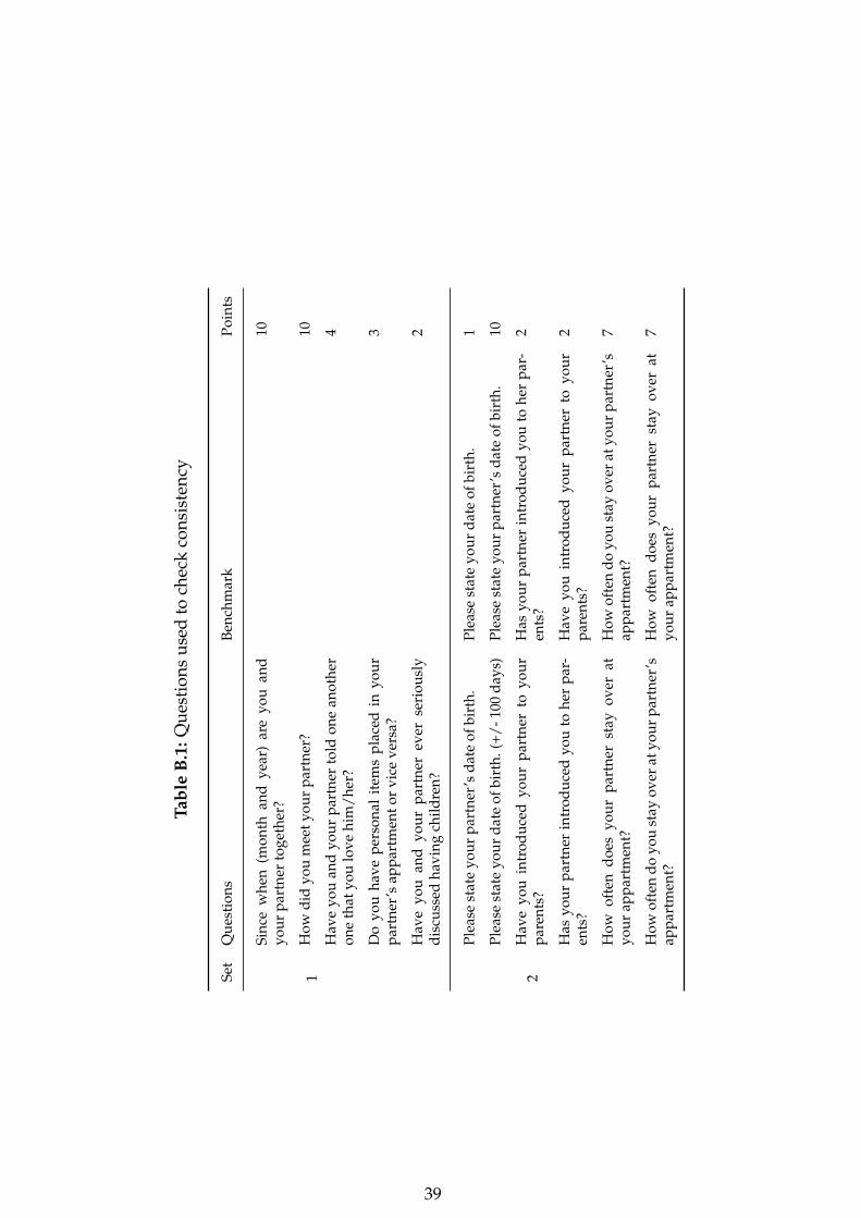
Tab

leB

.1:

Qu

esti

ons

use

dto

chec

kco

nsi

sten

cy

Set

Qu

esti

ons

Ben

chm

ark

Poi

nts

1

Sin

cew

hen

(mon

than

dye

ar)

are

you

and

you

rp

artn

erto

geth

er?

10

How

did

you

mee

tyo

ur

par

tner

?10

Hav

eyo

uan

dyo

ur

par

tner

told

one

anot

her

one

that

you

love

him

/h

er?

4

Do

you

hav

ep

erso

nal

item

sp

lace

din

you

rp

artn

er’s

app

artm

ent

orvi

ceve

rsa?

3

Hav

eyo

uan

dyo

ur

par

tner

ever

seri

ousl

yd

iscu

ssed

hav

ing

chil

dre

n?

2

2

Ple

ase

stat

eyo

ur

par

tner

’sd

ate

ofbi

rth

.P

leas

est

ate

you

rd

ate

ofbi

rth

.1

Ple

ase

stat

eyo

ur

dat

eof

birt

h.(

+/

-100

day

s)P

leas

est

ate

you

rp

artn

er’s

dat

eof

birt

h.

10

Hav

eyo

uin

trod

uce

dyo

ur

par

tner

toyo

ur

par

ents

?H

asyo

ur

par

tner

intr

odu

ced

you

toh

erp

ar-

ents

?2

Has

you

rp

artn

erin

trod

uce

dyo

uto

her

par

-en

ts?

Hav

eyo

uin

trod

uce

dyo

ur

par

tner

toyo

ur

par

ents

?2

How

ofte

nd

oes

you

rp

artn

erst

ayov

erat

you

rap

par

tmen

t?H

owof

ten

do

you

stay

over

atyo

ur

par

tner

’sap

par

tmen

t?7

How

ofte

nd

oyo

ust

ayov

erat

you

rp

artn

er’s

app

artm

ent?

How

ofte

nd

oes

you

rp

artn

erst

ayov

erat

you

rap

par

tmen

t?7

39

avoid overweighting the many “consistent” missing answers by partners who do not

cohabitate. Thus, the maximum consistency score is 58.

The boxplot below shows that the vast majority of couples achieve high consis-

tency rates (obtained by normalising the consistency score). In fact, three quarters

of the couples achieve at least 65.5% of the maximum score. The median couple

achieves 77.6%. Only 8 couples (fewer than 9%), achieve less than 50% of the score.

All analyses presented in the paper are unaffected if these couples are excluded.

Figure B.1: Couple’s normalised consistency score

Note: The boxplot shows the distribution of couples over the normalised consistency score. It iscalculated by dividing the number of points a couple scored in answering the questions documented

in Table B.1 over the maximum number of points.

chose to assign the maximum number that can be scored in a closed question.

40

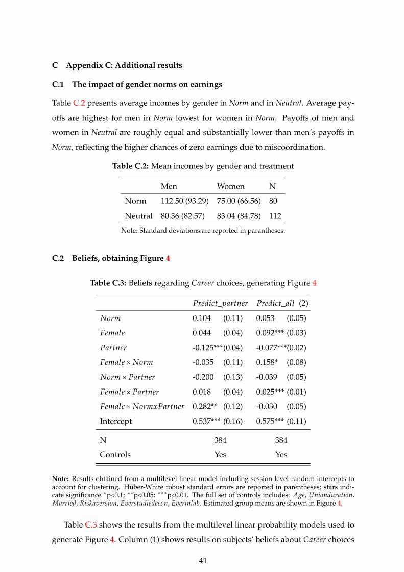
C Appendix C: Additional results

C.1 The impact of gender norms on earnings

Table C.2 presents average incomes by gender in Norm and in Neutral. Average pay-

offs are highest for men in Norm lowest for women in Norm. Payoffs of men and

women in Neutral are roughly equal and substantially lower than men’s payoffs in

Norm, reflecting the higher chances of zero earnings due to miscoordination.

Table C.2: Mean incomes by gender and treatment

Men Women N

Norm 112.50 (93.29) 75.00 (66.56) 80

Neutral 80.36 (82.57) 83.04 (84.78) 112

Note: Standard deviations are reported in parantheses.

C.2 Beliefs, obtaining Figure 4

Table C.3: Beliefs regarding Career choices, generating Figure 4

Predict_partner Predict_all (2)

Norm 0.104 (0.11) 0.053 (0.05)

Female 0.044 (0.04) 0.092*** (0.03)

Partner -0.125***(0.04) -0.077***(0.02)

Female ×Norm -0.035 (0.11) 0.158* (0.08)

Norm × Partner -0.200 (0.13) -0.039 (0.05)

Female × Partner 0.018 (0.04) 0.025*** (0.01)

Female ×NormxPartner 0.282** (0.12) -0.030 (0.05)

Intercept 0.537*** (0.16) 0.575*** (0.11)

N 384 384

Controls Yes Yes

Note: Results obtained from a multilevel linear model including session-level random intercepts toaccount for clustering. Huber-White robust standard errors are reported in parentheses; stars indi-cate significance ∗p<0.1; ∗∗p<0.05; ∗∗∗p<0.01. The full set of controls includes: Age, Unionduration,Married, Riskaversion, Everstudiedecon, Everinlab. Estimated group means are shown in Figure 4.

Table C.3 shows the results from the multilevel linear probability models used to

generate Figure 4. Column (1) shows results on subjects’ beliefs about Career choices

41

of the partner they are paired with, i.e. the dependent variable is an indicator that

equals one when a subject predicted that their partner chose Career and zero other-

wise. Explanatory variables refer to the subject who is making predictions, i.e. the

indicator Female is one if the subject is female (i.e., predicting the Career choice of her

male partner), Partner is one if she predicting the behaviour of her real partner, etc.

Column (2) shows results on subjects’ beliefs about other players in their session,

i.e. the dependent variable is a continuous and ranges from zero to one and measures

the predicted fraction of subjects of the opposite gender in the session that chose

Career. Again, the indicator Female is equal to one for women who were predicting

the fraction of men (paired with strangers) choosing Career. Partner is equal one

for predictions referring to session participants playing with their real partner, etc.

Estimated group means from these models are visualised in Figure 4 in Section 5.1,

which provides a detailed discussion of the results.

Figure C.2: Proportion of subjects with correct beliefs about their partner’s Careerchoice

Note: Proportions, p-values, and 95% confidence intervals (shown by whiskers) are calculated from amultilevel linear model with Huber-White robust standard errors, holding all other controls ( Age,

Unionduration, Married, Riskaversion, Everstudiedecon, Everinlab) constant at their average.

Another interesting question regarding subjects’ beliefs is the extent to which they

are accurate. To assess this, Figure C.2 shows the predicted proportions of subjects

who correctly predicted their partner’s Career choice, by gender and treatment. Es-

42

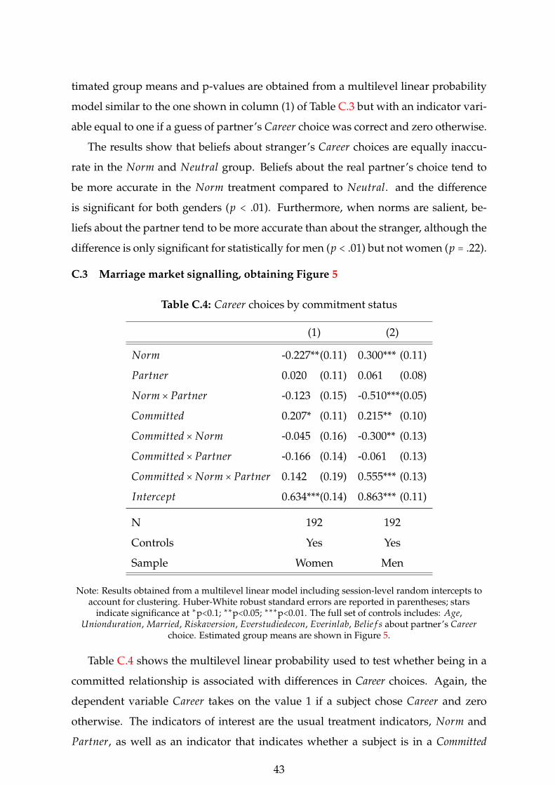
timated group means and p-values are obtained from a multilevel linear probability

model similar to the one shown in column (1) of Table C.3 but with an indicator vari-

able equal to one if a guess of partner’s Career choice was correct and zero otherwise.

The results show that beliefs about stranger’s Career choices are equally inaccu-

rate in the Norm and Neutral group. Beliefs about the real partner’s choice tend to

be more accurate in the Norm treatment compared to Neutral. and the difference

is significant for both genders (p < .01). Furthermore, when norms are salient, be-

liefs about the partner tend to be more accurate than about the stranger, although the

difference is only significant for statistically for men (p < .01) but not women (p = .22).

C.3 Marriage market signalling, obtaining Figure 5

Table C.4: Career choices by commitment status

(1) (2)

Norm -0.227**(0.11) 0.300*** (0.11)

Partner 0.020 (0.11) 0.061 (0.08)

Norm × Partner -0.123 (0.15) -0.510***(0.05)

Committed 0.207* (0.11) 0.215** (0.10)

Committed ×Norm -0.045 (0.16) -0.300** (0.13)

Committed × Partner -0.166 (0.14) -0.061 (0.13)

Committed ×Norm × Partner 0.142 (0.19) 0.555*** (0.13)

Intercept 0.634***(0.14) 0.863*** (0.11)

N 192 192

Controls Yes Yes

Sample Women Men

Note: Results obtained from a multilevel linear model including session-level random intercepts toaccount for clustering. Huber-White robust standard errors are reported in parentheses; stars

indicate significance at ∗p<0.1; ∗∗p<0.05; ∗∗∗p<0.01. The full set of controls includes: Age,Unionduration, Married, Riskaversion, Everstudiedecon, Everinlab, Belie f s about partner’s Career

choice. Estimated group means are shown in Figure 5.

Table C.4 shows the multilevel linear probability used to test whether being in a

committed relationship is associated with differences in Career choices. Again, the

dependent variable Career takes on the value 1 if a subject chose Career and zero

otherwise. The indicators of interest are the usual treatment indicators, Norm and

Partner, as well as an indicator that indicates whether a subject is in a Committed

43

relationship. Column (1) shows the estimation results for the female, column (2) for

the male sample. The estimated group means resulting from these regression are

summarised in Figure 5 and discussed in detail in Section 5.2.

C.4 Robustness

Table C.5 presents a collection of robustness checks for the main outcome variable,

the indicator for choosing Career.31 The first column simply reproduces the results

from full model presented in column 3 of Table 4. In column (2) a control for beliefs

about partner’s Career choice is added. This does not alter the results qualitatively,

but coefficients gain precision.32 The coefficient on the variable Belie f , which is not

shown in the table, shows the expected sign and is statistically significant: The like-

lihood likelihood that a subject chooses Career decreases by almost 44 percentage

points if they believe that their partner chose Career (p < .001).

Column (3) shows the same regression but using a multilevel logit instead of a

multilevel linear probability model. Again, this does not affect the results.33 Ad-

ditional checks confirmed that predicted group-level probabilities obtained from the

model are also very similar (results available upon request). The fourth model shown

in columns (4) controls for possible order effects by including an indicator variable

for the second round. Again, this barely effects the results. In addition, the coefficient

on the Round2 dummy, not shown in the table, is insignificant (p = .24).

Finally, column (5) shows the results for the restricted sample of first-time par-

ticipants. The regression includes the same set of controls as those shown in the

preceding column (4), except for the indicator variable Everinlab, which is zero for

everyone in the restricted sample and hence is dropped. While the results remain

qualitatively similar, some lose precision. This is not surprising given that the over-

31Results for the multinomial logistic regressions on the coordination Outcome are similarly robustto different specifications, inclusion of additional controls, alternative sample restrictions. Results areavailable upon request.

32One notable exception is the coefficient on Partner, which in Column (1) indicated that there is asignificant difference in (men’s) Career choices when paired with their partner vs. when paired witha stranger even in the Neutral treatment. This effect reassuringly loses magnitude and significanceafter controlling for beliefs. Importantly, the main result discussed in the text—the difference in men’sresponse to the salience of Norms when matched with a partner vs. a stranger, captured by the inter-action on Norm × Partner actually increases both in magnitude and significance when controlling forbeliefs. Similarly, the coefficent on Norm becomes (marginally) significant, too, indicating that menpaired with strangers do actually respond to the salience of Norms as predicted, by choosing Career ata higher rate.

33The table reports coefficients, as the transformation to marginal effects is not feasible for modelsinvolving interactions of factor variables.

44

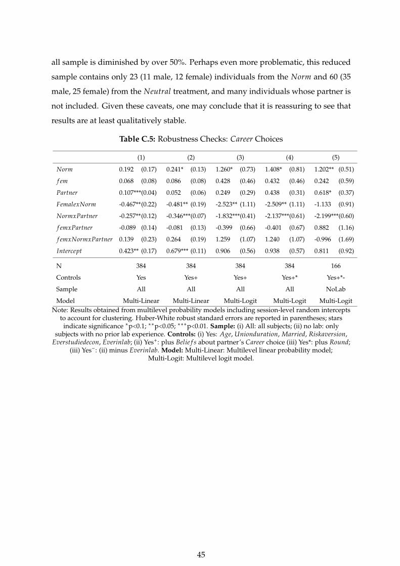
all sample is diminished by over 50%. Perhaps even more problematic, this reduced

sample contains only 23 (11 male, 12 female) individuals from the Norm and 60 (35

male, 25 female) from the Neutral treatment, and many individuals whose partner is

not included. Given these caveats, one may conclude that it is reassuring to see that

results are at least qualitatively stable.

Table C.5: Robustness Checks: Career Choices

(1) (2) (3) (4) (5)

Norm 0.192 (0.17) 0.241* (0.13) 1.260* (0.73) 1.408* (0.81) 1.202** (0.51)

f em 0.068 (0.08) 0.086 (0.08) 0.428 (0.46) 0.432 (0.46) 0.242 (0.59)

Partner 0.107***(0.04) 0.052 (0.06) 0.249 (0.29) 0.438 (0.31) 0.618* (0.37)

FemalexNorm -0.467**(0.22) -0.481** (0.19) -2.523** (1.11) -2.509** (1.11) -1.133 (0.91)

NormxPartner -0.257**(0.12) -0.346***(0.07) -1.832***(0.41) -2.137***(0.61) -2.199***(0.60)

f emxPartner -0.089 (0.14) -0.081 (0.13) -0.399 (0.66) -0.401 (0.67) 0.882 (1.16)

f emxNormxPartner 0.139 (0.23) 0.264 (0.19) 1.259 (1.07) 1.240 (1.07) -0.996 (1.69)

Intercept 0.423** (0.17) 0.679*** (0.11) 0.906 (0.56) 0.938 (0.57) 0.811 (0.92)

N 384 384 384 384 166

Controls Yes Yes+ Yes+ Yes+* Yes+*-

Sample All All All All NoLab

Model Multi-Linear Multi-Linear Multi-Logit Multi-Logit Multi-LogitNote: Results obtained from multilevel probability models including session-level random intercepts

to account for clustering. Huber-White robust standard errors are reported in parentheses; starsindicate significance ∗p<0.1; ∗∗p<0.05; ∗∗∗p<0.01. Sample: (i) All: all subjects; (ii) no lab: only

subjects with no prior lab experience. Controls: (i) Yes: Age, Unionduration, Married, Riskaversion,Everstudiedecon, Everinlab; (ii) Yes+: plus Belie f s about partner’s Career choice (iii) Yes*: plus Round;

(iii) Yes−: (ii) minus Everinlab. Model: Multi-Linear: Multilevel linear probability model;Multi-Logit: Multilevel logit model.

45

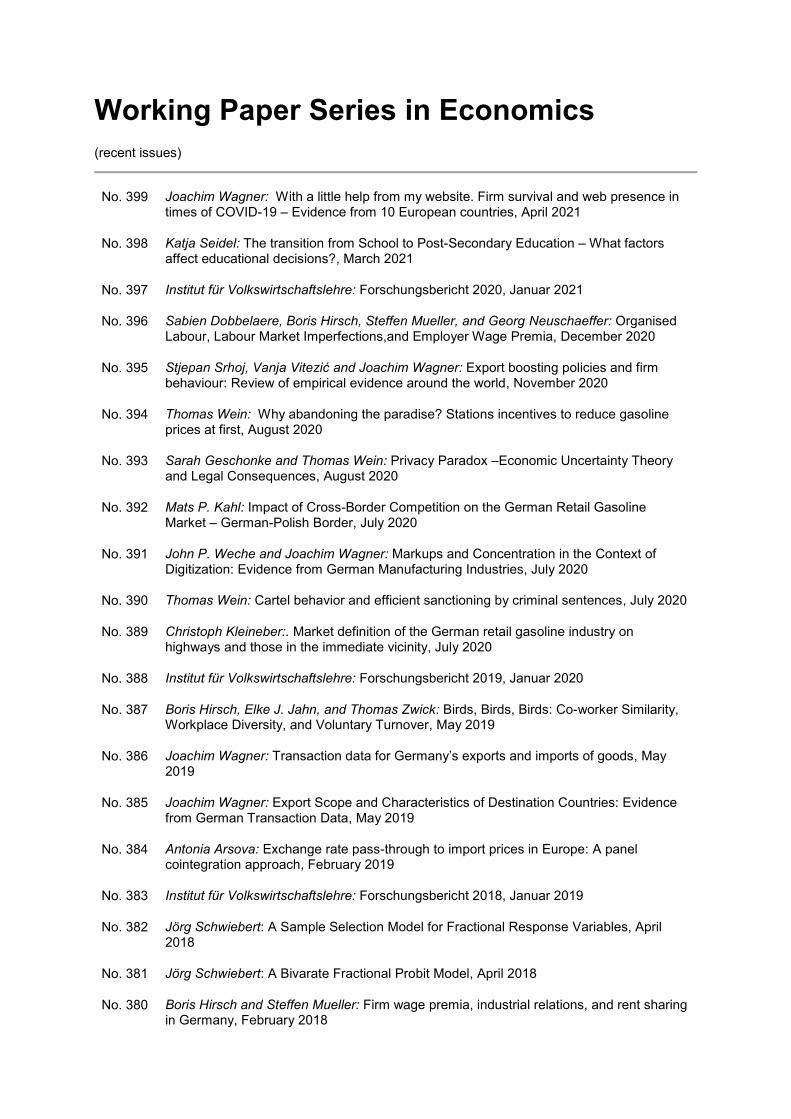
Working Paper Series in Economics

(recent issues)

No. 399 Joachim Wagner: With a little help from my website. Firm survival and web presence in times of COVID-19 – Evidence from 10 European countries, April 2021

No. 398 Katja Seidel: The transition from School to Post-Secondary Education – What factors affect educational decisions?, March 2021

No. 397 Institut für Volkswirtschaftslehre: Forschungsbericht 2020, Januar 2021

No. 396 Sabien Dobbelaere, Boris Hirsch, Steffen Mueller, and Georg Neuschaeffer: Organised Labour, Labour Market Imperfections,and Employer Wage Premia, December 2020

No. 395 Stjepan Srhoj, Vanja Vitezić and Joachim Wagner: Export boosting policies and firm behaviour: Review of empirical evidence around the world, November 2020

No. 394 Thomas Wein: Why abandoning the paradise? Stations incentives to reduce gasoline prices at first, August 2020

No. 393 Sarah Geschonke and Thomas Wein: Privacy Paradox –Economic Uncertainty Theory and Legal Consequences, August 2020

No. 392 Mats P. Kahl: Impact of Cross-Border Competition on the German Retail Gasoline Market – German-Polish Border, July 2020

No. 391 John P. Weche and Joachim Wagner: Markups and Concentration in the Context of Digitization: Evidence from German Manufacturing Industries, July 2020

No. 390 Thomas Wein: Cartel behavior and efficient sanctioning by criminal sentences, July 2020

No. 389 Christoph Kleineber:. Market definition of the German retail gasoline industry on highways and those in the immediate vicinity, July 2020

No. 388 Institut für Volkswirtschaftslehre: Forschungsbericht 2019, Januar 2020

No. 387 Boris Hirsch, Elke J. Jahn, and Thomas Zwick: Birds, Birds, Birds: Co-worker Similarity, Workplace Diversity, and Voluntary Turnover, May 2019

No. 386 Joachim Wagner: Transaction data for Germany’s exports and imports of goods, May 2019

No. 385 Joachim Wagner: Export Scope and Characteristics of Destination Countries: Evidence from German Transaction Data, May 2019

No. 384 Antonia Arsova: Exchange rate pass-through to import prices in Europe: A panel cointegration approach, February 2019

No. 383 Institut für Volkswirtschaftslehre: Forschungsbericht 2018, Januar 2019

No. 382 Jörg Schwiebert: A Sample Selection Model for Fractional Response Variables, April 2018

No. 381 Jörg Schwiebert: A Bivarate Fractional Probit Model, April 2018

No. 380 Boris Hirsch and Steffen Mueller: Firm wage premia, industrial relations, and rent sharing in Germany, February 2018

No. 379 John P. Weche and Achim Wambach: The fall and rise of market power in Europe, January 2018

No.378: Institut für Volkswirtschaftslehre: Forschungsbericht 2017, Januar 2018

No.377: Inna Petrunyk and Christian Pfeifer: Shortening the potential duration of unemployment benefits and labor market outcomes: Evidence from a natural experiment in Germany, January 2018

No.376: Katharina Rogge, Markus Groth und Roland Schuhr: Offenlegung von CO2-Emissionen und Klimastrategien der CDAX-Unternehmen – eine statistische Analyse erklärender Faktoren am Beispiel der CDP-Klimaberichterstattung, Oktober 2017

No.375: Christoph Kleineberg und Thomas Wein: Verdrängungspreise an Tankstellen?, September 2017

No.374: Markus Groth, Laura Schäfer und Pia Scholz: 200 Jahre „On the Principles of Political Economy and Taxation“ – Eine historische Einordnung und Würdigung, März 2017

No.373: Joachim Wagner: It pays to be active on many foreign markets - Profitability in German multi-market exporters and importers from manufacturing industries, March 2017

No.372: Joachim Wagner: Productivity premia for many modes of internationalization - A replication study of Békes / Muraközy, Economics Letters (2016), March 2017 [published in: International Journal for Re-Views in Empirical Economics - IREE, Vol. 1 (2017-4)]

No.371: Marius Stankoweit, Markus Groth and Daniela Jacob: On the Heterogeneity of the Economic Value of Electricity Distribution Networks: an Application to Germany, March 2017

No.370: Joachim Wagner: Firm size and the use of export intermediaries. A replication study of Abel-Koch, The World Economy (2013), January 2017 [published in: International Journal for Re-Views in Empirical Economics - IREE, Vol. 1 (2017-1)]

No.369: Joachim Wagner: Multiple import sourcing First evidence for German enterprises from manufacturing industries, January 2017 [published in : Open Economies Review 29 (2018), 1, 165-175]

No.368: Joachim Wagner: Active on many foreign markets A portrait of German multi-market exporters and importers from manufacturing industries, January 2017 [published in: Jahrbücher für Nationalökonomie und Statistik 238 (2018), 2, 157-182]

No.367: Institut für Volkswirtschaftslehre: Forschungsbericht 2016, Januar 2017

No.366: Tim W. Dornis and Thomas Wein: Trademarks, Comparative Advertising, and Product Imitations: An Untold Story of Law and Economics, September 2016

No.365: Joachim Wagner: Intra-good trade in Germany: A first look at the evidence, August 2016 [published in: Applied Economics 49 (2017), 57, 5753-5761]

No.364: Markus Groth and Annette Brunsmeier: A cross-sectoral analysis of climate change risk drivers based on companies’ responses to the CDP’s climate change information request, June 2016

No.363: Arne Neukirch and Thomas Wein: Collusive Upward Gasoline Price Movements in Medium-Sized German Cities, June 2016

No.362: Katja Seidel: Job Characteristics and their Effect on the Intention to Quit Apprenticeship., May 2016

(see www.leuphana.de/institute/ivwl/working-papers.html for a complete list)

No.361: Katja Seidel: Apprenticeship: The Intention to Quit and the Role of Secondary Jobs in It., May 2016

No.360: Joachim Wagner: Trade costs shocks and lumpiness of imports: Evidence from the Fukushima disaster, May 2016 [published in: Economics Bulletin 37 (2017), 1, 149-155]

No.359: Joachim Wagner: The Lumpiness of German Exports and Imports of Goods, April 2016 [published in: Economics - The Open-Access, Open-Assessment E-Journal 10, 2016-21]

No.358: Ahmed Fayez Abdelgouad: Exporting and Workforce Skills-Intensity in the Egyptian Manufacturing Firms: Empirical Evidence Using World Bank Firm-Level Data for Egypt, April 2016

No.357: Antonia Arsova and Deniz Dilan Karaman Örsal: An intersection test for the cointegrating rank in dependent panel data, March 2016

No.356: Institut für Volkswirtschaftslehre: Forschungsbericht 2015, Januar 2016

No.355: Christoph Kleineberg and Thomas Wein: Relevance and Detection Problems of Margin Squeeze – The Case of German Gasoline Prices, December 2015

No.354: Karsten Mau: US Policy Spillover(?) - China's Accession to the WTO and Rising Exports to the EU, December 2015

No.353: Andree Ehlert, Thomas Wein and Peter Zweifel: Overcoming Resistance Against Managed Care – Insights from a Bargaining Model, December 2015

No.352: Arne Neukirch und Thomas Wein: Marktbeherrschung im Tankstellenmarkt - Fehlender Binnen- und Außenwettbewerb an der Tankstelle? Deskriptive Evidenz für Marktbeherrschung, Dezember 2015

No.351: Jana Stoever and John P. Weche: Environmental regulation and sustainable competitiveness: Evaluating the role of firm-level green investments in the context of the Porter hypothesis, November 2015

No.350: John P. Weche: Does green corporate investment really crowd out other business investment?, November 2015

No.349: Deniz Dilan Karaman Örsal and Antonia Arsova: Meta-analytic cointegrating rank tests for dependent panels, November 2015

No.348: Joachim Wagner: Trade Dynamics and Trade Costs: First Evidence from the Exporter and Importer Dynamics Database for Germany, October 2015 [published in: Applied Economics Quarterly 63 (2017), 2, 137-159]

No.347: Markus Groth, Maria Brück and Teresa Oberascher: Climate change related risks, opportunities and adaptation actions in European cities – Insights from responses to the CDP cities program, October 2015

No.346: Joachim Wagner: 25 Jahre Nutzung vertraulicher Firmenpaneldaten der amtlichen Statistik für wirtschaftswissenschaftliche Forschung: Produkte, Projekte, Probleme, Perspektiven, September 2015 [publiziert in: AStA Wirtschafts- und Sozialstatistisches Archiv 9 (2015), 2, 83-106]

No.345: Christian Pfeifer: Unfair Wage Perceptions and Sleep: Evidence from German Survey Data, August 2015

Leuphana Universität Lüneburg

Institut für Volkswirtschaftslehre

Postfach 2440

D-21314 Lüneburg

Tel.: ++49 4131 677 2321

email: korf@leuphana.de

www.leuphana.de/institute/ivwl/working-papers.html