of econometrics - cemfiarellano/arellano-bover-1995.pdf · a closely related transformation has...

JOIJIXNAL OF Econometrics

Journal of Econometrics 68 (1995) 29-51

Another look at the instrumental variable estimation of error-components models

Manuel Areliano *va, Olympia Boverb

“CEMFI, 28014 Madrid, Spain bResearch Department, Bank of Spain, 28014 Madrid, Spain

Abstract

This article develops a framework for efficient IV estimators of random effects models with information in levels which can accommodate predetermined variables. Our formulation clarifies the relationship between the existing estimators and the role of transformations in panel data models. We characterize the valid transformations for relevant models and show that optimal estimators are invariant to the transformation used to remove individual effects. We present an alternative transformation for models with predetermined instruments which preserves the orthogonality among the errors. Finally, we consider models with predetermined variables that have constant correlation with the effects and illustrate their importance with simulations.

Key words: Dynamic panel data; Predetermined instrumental variables; Orthogonal deviations; Unrestricted covariance matrix; Unit roots JEL classijcation: C23

1. Introduction

The static error components model with both time-invariant and time- varying explanatory variables allowing for the correlation of some of these

* Corresponding author.

An earlier version of this paper was presented at the World Congress of the Econometric Society in

Barcelona, August 1990, and at the Canadian Econometrics Study Group in Guelph, September

1990. It circulated as Centre for Economic Performance Discussion Paper No. 7 (London School of

Economics, August 1990). We thank Steve Bond, David Card, Gary Chamberlain, Franc0 Peracchi.

and specially Peter Schmidt for useful comments. All remaining errors are our own.

0304~4076/95/$09.50 $2,;: 1995 Elsevier Science S.A. All rights reserved

SSDI 030440769401642 D

30 M. Arellano. 0. Bover / Journal of Econometrics 68 (1995) 29-51

variables with the unobservable individual effects was first considered by

Hausman and Taylor (1981) ~ hereafter HT. Bhargava and Sargan (1983) _ hereafter BS - studied the estimation of dynamic error components models,

and also considered a model which contained a lagged dependent variable and

allowed for correlation between some of the regressors and the effects. Sub- sequently, Amemiya and MaCurdy (1986) - hereafter AM - and Breusch,

Mizon, and Schmidt (1989) ~ hereafter BMS - developed alternative instrumental variable (IV) estimators of the HT model that are more efficient than the

original HT estimator. On the other hand, Anderson and Hsiao (1982), Holtz- Eakin, Newey, and Rosen (1988) and Arellano and Bond (1991) amongst others, considered the estimation of models with predetermined but no strictly

exogenous variables by IV methods using lagged values of the predetermined variables as instruments for the equations in first differences. In these models it is

usually maintained that all the explanatory variables are potentially correlated with the individual effects and therefore only estimators based on deviations of

the original observations can be consistent. However, if there are instruments available that are not correlated with the effects, the levels of the variables contain information concerning the parameters of interest which if exploited could improve, sometimes crucially, the efficiency of the resulting estimates. In addition, this information in the levels may be sufficient to identify the coeffi-

cients of time-invariant explanatory variables that are correlated with the effects. The purpose of this paper is to develop a framework for efficient IV estimators

with information in levels which is capable of accommodating models with lagged dependent variables and other predetermined variables. In Section 2 we

present a generalised method of moments formulation of HT, AM, and BMS- like estimators. Each particular model gives rise to a set of orthogonality restrictions on which estimation is to be based. We follow Amemiya and

MaCurdy in exploiting transformations of the original equations in order to obtain convenient expressions of these restrictions. However, we formulate the matrices of instruments as block-diagonal matrices with as many blocks as the

total number of time periods. In this way we can show that the optimal estimators are invariant to the choice of transformation. Another advantage of proceeding in this way is that we can obtain HT, AM, and BMS estimators with

nonstandard or unrestricted covariance matrix without having to specify the appropriate GLS transformation and subsequent changes to the instrument set to avoid inconsistencies. As noted by AM, since different instruments are only valid for subsets of equations, GLS transformations are sensitive in this context: a particular IV matrix that is valid for some GLS transformation of the model may be invalid under a different GLS transformation. By specifying an IV matrix that effectively lists all the individual moment restrictions available we avoid this problem. We also calculate the Fisher information bound for the parameters of a conditional moment specification of the model in order to assess the efficiency of the class of GMM estimators formulated in Section 2.

M. Arellano. 0. Rover / Journal of Econometrics 68 (1995j 29-51 31

Section 3 shows how the previous framework can easily accommodate dynamic models, and other models with predetermined variables and information in levels. We discuss an IV estimator which is asymptotically equivalent to the limited information maximum likelihood (LIML) estimator with unrestricted covariance matrix and correlated exogenous variables of BS. This clarifies the relationship between HT/AM/BMS and BS. We also extend these estimators to include lags of predetermined variables as additional instruments. We character- ise the class of valid transformations in this context and show the invariance of the optimal estimators to a particular choice of transformation. We argue that a computationally convenient transformation for these models is forward orthogonal deviations. A closely related transformation has been used by Hayashi and Sims (1983) for time series models. This transformation leads to simple expressions of the estimators in terms of the vectors of instruments corresponding to individual time periods, and so it avoids the need to operate with the full block-diagonal IV matrix which may have an excessively large number of columns. Section 3 also formulates a GMM estimator for a general model with predetermined variables and information in levels.

Section 4 considers a model with predetermined variables that have constant correlation with the individual effects. As an illustration of the potential of these constraints, we report Monte Carlo simulations of IV estimators of a first-order stationary autoregression with random effects that exploit the orthogonality restrictions in levels. An estimator that only uses the restrictions in first differences is also simulated for comparisons. The section concludes with some remarks on the usefulness of predetermined variables that have constant correlation with the effects for the testing of unit roots in short panels. Finally, Section 5 contains the conclusions of the paper.

2. A method of moments formulation of Hausman-Taylor and related estimators with unrestricted covariance matrix

Let us consider the model

J’if = PXif + y’h + Uit> t=l,..., T, i=l...., N,

Uit = Vi + uif7

E(Ui,Ixi,, ... TXiT,f;.+qi) = 0.

SO that the variables Xir andfi are assumed to be strictly exogenous given the unobservable individual effect vi. Under standard conditions, this assumption identifies p but not y. The identification of y is based on the following assumption:

32 M. Arellano, 0. Bover / Journal of Econometrics 68 (1995) 29-51

where we are using the partitions xig = (x;it, x;i,)’ andJ = (f;i,f;i)‘. Throughout, T is small and N is large. This model can be regarded as an intermediate case between the ‘fixed effects’ model in which all the explanatory variables are potentially correlated with the effects and therefore only estimators based on deviations of the observations can be consistent, and the standard uncorrelated ‘random effects’ model in which xtil = xit and $1; =1;.

It is convenient to re-write (1) in the form

yi = WiS + Ui, (3)

where yi = (yir, . . . ,yir)‘, ai = (#iI, . . . ,UiT)‘, S = (/I’, y’)‘, Wi = (Xi I Lfi’)3 Xi = (Xi12 ...) XiT)' and I is a T x 1 vector of ones. Below, we also make use of the notation X,! = T -‘z’X~ = (X;i, X;i) and the vectors vi = (ail, . . . ,Dir)‘, Xi = (X[l, ... ,xiT)', and wi = (xi,h')'.

In general, the matrix E(uiuf 1 Wi) will be unrestricted and depend on Wi:

E(aiaj / Wi) = E(aiaf 1 WJ + E(rlZ 1 Wi) II’ = f2(Wi).

However, here we emphasize two cases with cross-sectional homoskedasticity in the sense that E(niU! 1 Wi) = E(uiul).’ Firstly, the case of a constant unrestricted Sz, which allows for the possibility of autocorrelation and time series heteroskedasticity of arbitrary form in the ait. Secondly, the traditional error components specification given by Sz = 02ZT + afzz’, where IT is the identity matrix of order T.

We then transform the system of T equations using a nonsingular T x T transformation matrix,

H= K

[ 1 T-1,’ ’

where K is any (T - 1) x T matrix of rank (T - 1) such that Kt = 0. For example, K could be the first difference operator or the first (T - 1) rows of the within-group operator. The transformed errors are given by

u+ = Hui = KUi

[ 1 iii .

This class of transformations performs a decomposition between ‘within- group’ and ‘between-group’ variation which is helpful in order to implement

’ We assume that E(q,) = E(E(qi/ w,)) = 0. Notice that, provided the model contains a constant

term, there is no loss of generality in this assumption. Thus, although it is always true that

E(u;u[) = var(u,) = var(uJ + var(qJn’, in general E(uiu; 1 wi) and var(uil w,) = var (yil wi) will differ as follows:

E(u,& wi) = var(uiIwi) + (E(qil wi))’ 11’

M. Arellano, 0. Bover 1 Journal of Econometrics 68 (1995) 29-51 33

orthogonality restrictions implied by the model. Specifically, since the first (7’ - 1) errors do not contain vi, all exogenous variables (as well as nonlinear functions of those variables) are valid instruments for the first (T - 1) equations. Then, if mi denotes a vector of a subset of variables of wi (or linear combinations of those variables) assumed to be uncorrelated in levels and such that dim(mJ > dim(y), a valid IV matrix for the complete transformed system is

W; 0

&= . . I. 1. W;

0 rni

We can now write down the optimal GMM estimator of 6 with constant s2 based on the moment equations,

E(Z1Hui) = 0,

which is given by --- ---

8 = [N”A’Z(Z’HQH’Z)- ‘Z’HW] - ’ W’R’Z(Z’HSZH’Z)-‘Z’Ry, (3

where W = (W; . . . Wa)‘, y = (y; ,.. yk)‘, Z = (Z; ___ Zh)‘, R = IN Q H, and Q = IN @ ft. In practice, the covariance matrix of the transformed system Q+ = Hi2H’ will be replaced by a consistent estimator. An unrestricted estimator of Q2+ takes the form

where the L?+ are residuals based on consistent preliminary estimates. Alterna- tively, we consider a restricted estimate 6’ = H6H’ with d = ~7’1~ + 5:~‘. where cF2 and 6; denote consistent estimates of 0’ and g,” .

The estimator of HT is 8 with 6’ and

mi = (f;i, Xii)‘,

whereas the estimator of AM is 8 with fi’ and

BS and BMS also exploited the additional moment restrictions that arise if it is assumed that the correlation between x2it and vi is constant over time. In this case, the deviations from time means )72il = XZir - Xii are valid instruments for the last equation of the transformed system. A stronger conditional expectation version of this assumption along the lines of (2) is

E(qiIxii,fii> 2zi) = 0. (6)


Setting

and using fii+, 8 gives the estimator of BMS. Moreover, if all variables are

uncorrelated with the effects, we can set mi = Wi in which case 8 with 6’ becomes the GLS estimator of Balestra and Nerlove (1966). On the other hand,

if all variables are correlated with the effects, the levels equation drops out, the coefficients 1’ are unidentified and estimation of /I is based on E(Z;iKUi) = 0 with Zdi = ICT_ i, @ wf. In the case of restricted Sz since KCX’ = o*KK ‘, letting

R=I,@K,X=(X; . . . Xh)‘, and Zd = (Z;, . Z;,)‘, the resulting estimator

is

p = [x’K’Z,(Z;KR’Z,)) iZ$X] - l x’R’Z,(Z;KK’Z,)- lz;Ky,

which can be shown to coincide with the within-group estimator. It is interesting to notice that having chosen a block-diagonal form for Zi, 8 is

invariant to the choice of transformation K. To prove this assertion we can use the following simple fact in GMM estimation. The optimal estimator of 0 based

on E[&(@] = 0 minimizes

S = (Cisi)‘A- ’ (Cisi),

where a is a consistent estimator of E(4ii”I). If we now consider 5: = F<i where F is a nonsingular transformation matrix, it turns out that the optimal estimator

of 8 based on 57 that minimizes

S* = (Ci5*)‘AI*-’ (Ci~*)

is numerically the same estimator as the one based on ti provided that

a* = F/1F’ since s = s*. In our case

where p1 and p2 are the number of elements in wi and mi, respectively, and the vet operator stacks the elements of a matrix by rows. Suppose that an alternative transformation H* = (K*’ k*z’)’ is used. Letting K* = @K and k* = ‘pT_’ we can write

where

F= @OIpl 0

0 1 ‘PIP, .

So that any valid transformation leads to the same estimator.

M. Arellano. 0. Bover 1 Journal of Econometrics 68 (I 995) 29-51 35

This is useful because in this way we can obtain HT, AM, and BMS-like estimators easily with various specifications for L? without having to specify the appropriate K ‘I2 transformation and subsequent changes to the instrument set

to avoid inconsistencies. It also provides a natural framework to extend the HT-type of estimators to cases where there are predetermined variables as we shall see below.

If L?+ is estimated as d+, straightforward manipulations reveal that (5) can be written as

~ = [ciwlQwi + 82T~iwim! (Cimiml)-‘~imiwl]-’

X [ciw!Qyi + 8’TCiwiml (~imim!)-‘~imivi]-‘, (8)

which produces more familiar expressions of the HT, AM, and BMS estimators for the corresponding choices of mi (details available in the Appendix).’ In this

expression Q is the within-group operator:

Q = IT - zr’/T = K’(KK’)- ‘K,

Wi = WllJT and 8’ = e2/(6’ + Tc?;).

As explained in the Appendix, in this case it is possible to simplify the form of Zi without changing the estimator.

The obvious advantage of the formulation (5) is that if we replace the error components estimator a+ by an unrestricted estimator 8+, we obtain alternative HT, AM, or BMS-type estimators which are as efficient asymptotically as the versions in (8) when E(Uirf) = a21r and strictly more efficient

when E(UiOj) # a2ZT. Moreover, with cross-sectional heteroskedasticity further efficiency can be achieved using a GMM estimator of the type discussed by

Chamberlain (1982), Hansen (1982) and White (1982) which would replace the

term (CiZ;Q+Zi) in (5) by a term of the form (ciZia’a”Zi).

The eJkienc_v boundfor 6

In order to assess the efficiency of the class of GMM estimators given in (5), it is useful to compare the inverse of the asymptotic variance matrix of s^ with the Fisher information bound for 6 based on the conditional moment restrictions (1 I and (2). Chamberlain (1992a), using a specification that includes (1) as a special case, shows that the bound for /I based on (1) is identical to the bound for fi based on the conditional moment restriction

E (K(Yi - X$)1 wli, w2i) = 0, (9)

‘A derivation of the estimators of HT. AM, and BMS as GMM estimators, in the case that noise is

iid, has been obtained independently by Ahn and Schmidt (1995).

36 M. Arellano. 0. Bover /Journal of Econometrics 68 (1995) 29-51

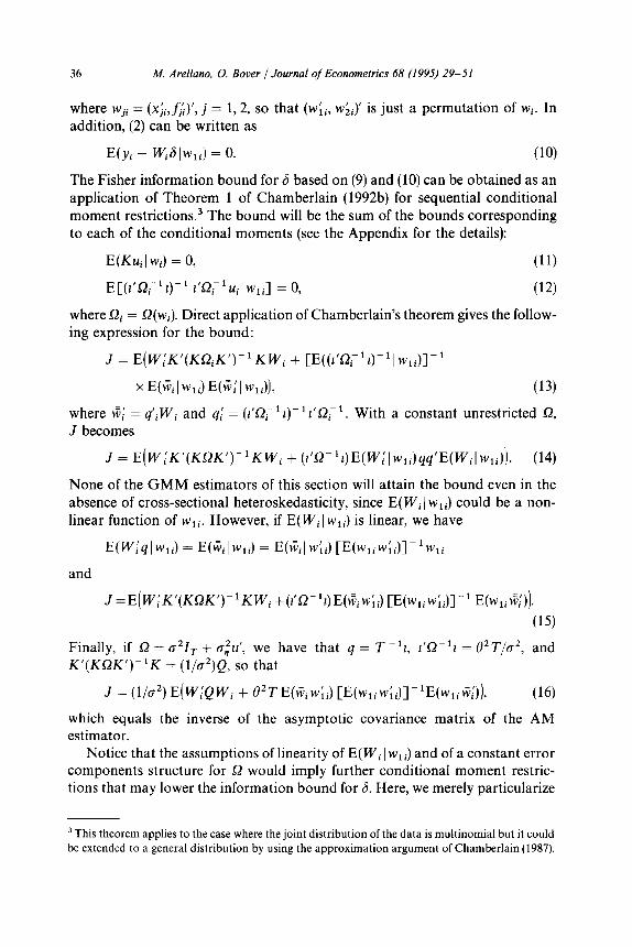
where wji = (xJi,fi)‘, j = 1,2, so that (W;i, W;i), is just a permutation of Wi. In addition, (2) can be written as

E(yi - Wi61Wli) = 0. (10)

The Fisher information bound for 6 based on (9) and (10) can be obtained as an application of Theorem 1 of Chamberlain (1992b) for sequential conditional moment restrictions3 The bound will be the sum of the bounds corresponding to each of the conditional moments (see the Appendix for the details):

E(Kui 1 Wi) = 0, (11)

E[(z’&!;‘~)-i ~‘s);‘uiIwii] = 0, (12)

where Szi = s2(wi). Direct application of Chamberlain’s theorem gives the following expression for the bound:

J = E(W!K’(KS2iK’)-‘KW, + [E((1’~2;‘1)-‘IWli)]-’

X E(~il Wli) E(~,I I Wli)), (13)

where $f = qliWi and q,! = (1’0; ‘I)- ’ z’sZLy ‘. With a constant unrestricted Q, J becomes

J = E(W!K’(KRK’)-‘KWi + (~‘52-‘I)E(WIJwli)qq’E(WilWli)). (14)

None of the GMM estimators of this section will attain the bound even in the absence of cross-sectional heteroskedasticity, since E( Wi ( Wli) could be a nonlinear function of Wli. However, if E( Wi I Wli) is linear, we have

E(Wlqlwii) = E(GiIwii) = E(Gilw;i) [E(wiiw;i)]-‘Wii

and

J=E(WjK’(K~2K’)-‘KWi+(l’a-‘Z)E(~iw;i) [E(WiiW;i)]-’ E(Wii${)).

(15)

Finally, if 52 = a2Zr + o,$r’, we have that q = T _ ‘1, z’Q_ ‘z = %2T/02, and K’(KL?K’)-‘K = (l/c’)Q, so that

J =(l/a2) E(WiQWi + %2TE(wiW;i) [E(wliw;i)]-‘E(wliw!)), (16)

which equals the inverse of the asymptotic covariance matrix of the AM estimator.

Notice that the assumptions of linearity of E( Wi I Wli) and of a constant error components structure for s2 would imply further conditional moment restrictions that may lower the information bound for 6. Here, we merely particularize

3 This theorem applies to the case where the joint distribution of the data is multinomial but it could

be extended to a general distribution by using the approximation argument of Chamberlain (1987).

M. Arellano, 0. Bover J Journal of Econometrics 68 (1995) 29-51 37

the bound for 6 based on (11) and (12) to the case where these additional restrictions happen to occur in the population but are not used in the calcu- lation of the bound.

We now turn to show that the inverse of the asymptotic covariance matrix of the GMM estimator given in (5) with unrestricted Q and the AM choice of instruments for the average equation mi = Wri, V/-l say, coincides with the information bound given in (15). Under standard regularity conditions

V- ’ = E(W;H’Zi) [E(ZIHQH’Zi)] - ’ E(ZiHW,).

On the other hand, since KXi equals the block Zr_ 1 @ w,f of Zi multiplied by a constant selection matrix, after straightforward manipulations (15) can be written as

J = E(WIH*‘Zi) [E(ZIH*S2H*‘Zi)]-‘E(ZfH*Wi),

with

H* zz K

[ 1 l’fi-’ .

We prove that I/-’ = J by showing that

Z;H* = F(Z;H), (17)

where F is a nonsingular matrix of constants. Firstly, notice that H* = @H with

@J= [

IT-1 0

l’i-PK’(KK’)-’ l’s)_ ll 1

Next, we consider a permutation of the columns of Zi = ZFP’ such that

Z*= I*QW;i [

IT- 10 w;i 1 0 .

Hence notice

and similarly

38 M. Arellano. 0. Bover j Journal of Economerrics 68 (1995) 29-51

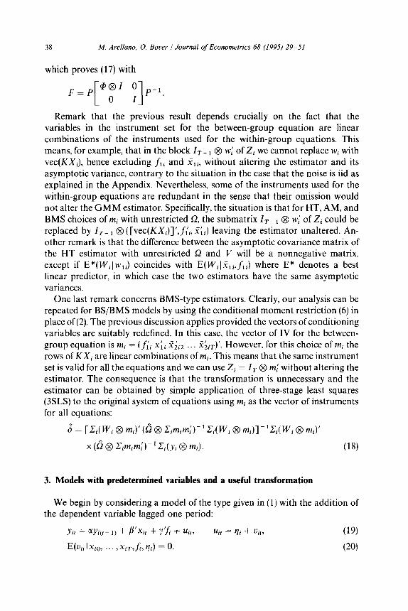
which proves (17) with

Remark that the previous result depends crucially on the fact that the variables in the instrument set for the between-group equation are linear combinations of the instruments used for the within-group equations. This means, for example, that in the block Ir_ 1 @ w( of Zi we cannot replace wi with vec(KXJ, hence excluding fii and Xii, without altering the estimator and its asymptotic variance, contrary to the situation in the case that the noise is iid as explained in the Appendix. Nevertheless, some of the instruments used for the within-group equations are redundant in the sense that their omission would not alter the GMM estimator. Specifically, the situation is that for HT, AM, and BMS choices of mi with unrestricted 52, the submatrix Ir- 1 @ wi of Zi could be replaced by I,_ i @ ([vec(KXJ]‘,ji’i, Xii) 1 eaving the estimator unaltered. An- other remark is that the difference between the asymptotic covariance matrix of the HT estimator with unrestricted Q and I/ will be a nonnegative matrix, except if E*(W,lwii) coincides with E(Wilxii,fii) where E* denotes a best linear predictor, in which case the two estimators have the same asymptotic variances.

One last remark concerns BMS-type estimators. Clearly, our analysis can be repeated for BS/BMS models by using the conditional moment restriction (6) in place of (2). The previous discussion applies provided the vectors of conditioning variables are suitably redefined. In this case, the vector of IV for the between- group equation is mi = (f;i X;i x";iz . . . Z';iT)'. However, for this choice of mi the rows of KXi are linear combinations of mi. This means that the same instrument set is valid for all the equations and we can use Zi = IT 0 mf without altering the estimator. The consequence is that the transformation is unnecessary and the estimator can be obtained by simple application of three-stage least squares (3SLS) to the original system of equations using mi as the vector of instruments for all equations:

~ = [Ci(Wi 0 mi)‘(B 0 Cimim!)-‘Ci(Wi 0 mi)]-‘Ci(Wi 0 mi)’

X(doCimimi)-'~i(yiOmi). (18)

3. Models with predetermined variables and a useful transformation

We begin by considering a model of the type given in (1) with the addition of the dependent variable lagged one period:

Yit = ccYi(t- 1) + PfXit + Y’J + uif, 41 = yli + uit, (19)

ECui, I XCO, .. . > XiTtfis Vi) = 0. (20)

M. Arellano. 0. Bover / Journal of Econometrics 68 (1995) 29-51 39

Assuming that t = 0 is observed and redefining the symbols in (3) as 6 = (a, p’, y’)’ and Wi = (yi(- I), Xi, I_&‘) with yi(-i) = (yio, . . . ,yi(T- I))‘, the expression given in (5) remains a consistent GMM estimator of 6 for this model, provided there are enough valid instruments to ensure identification. The form of the IV matrix Zi is the same as in Section 2, adjusting for the fact that t = 0 is now observed, SO that Wi = (x&, . . . , xiT,fi’) (notice the exclusion Of yi(- i, despite its presence in Wi). The same range of choices for mi are available depending on the assumptions concerning the dependence between ?i and subsets of the explanatory variables.

In particular, if mi = (f;i, Xii, Z;il, . . . , X”;iT), in view of the reasons explained for BMS-type cases above, the resulting estimator coincides with 3SLS and is therefore asymptotically equivalent to the LIML procedure with Sz unrestricted developed by Bhargava and Sargan. BS obtained their estimator as an application of subsystem LIML to the T equations (19X having completed the system with the reduced form equations,

YiO = XLJmi + EiO, f*i = nlmi + Eil, X2i = n2mi + Ei2r

and the identities

xZit = x2it + XZi, t=O,...,T-1.

It is well-known that subsystem LIML is asymptotically equivalent to subsystem 3SLS when 52 is unrestricted.

As in the static model, one polar case is the uncorrelated random effects specification with E(l?i Ixi,fi) = 0, SO that mi = Wi, which corresponds to the basic model of BS. At the other end, vi would be potentially correlated with all explanatory variables and there would be no instruments for the levels equation, which would drop out. This corresponds to the model and the 3SLS estimator discussed by Chamberlain (1984, pp. 12661267).

In the previous model, regardless of the existence of individual effects, unrestricted serial correlation in Dit implies that yi(f- i) is an endogenous variable. A different model, in which yi(t- i) is a predetermined variable given vi, replaces (20) by the following assumption:

E(tiit)Xi~fi~Vi~Yio~ . . ..Yi(t-~.) =O. (21)

Notice that (21) implies lack of serial dependence in the sense that E(Ui, 1 Vii.. Ui(f- i)) = 0. Orthogonality restrictions implied by this model can be easily incorporated in an estimator of the form of (5) provided that the transformation matrix K is upper-triangular in addition to the previous require- ments. In effect, with lack of autocorrelation in Uir and K upper-triangular it

40 M. Arellano. 0. Bover / Journal of Econometrics 68 (1995) 29-51

turns out that the transformed error in the equation for period t is independent of vi and (Vi13 . . . , oi(t- 1)) ~0 that (em, . . . , yi(, _ 1J are additional valid instruments for this equation. Hence giving rise to the following Zi matrix:

W! YiO 0

wf YiO Yil 1 Zi =I (22)

wl YiO .a* Yi(T-2)

0 mf

Estimators that rely on these types of restrictions have been discussed by Anderson and Hsiao (1982), Holtz-Eakin, Newey, and Rosen (1988), and Arel- lano and Bond (1991). These authors transformed the data using first differences and disregarded the levels in the absence of valid instruments for this equation (Arellano and Bond (p. 280) did, however, present a discussion of models with predetermined and strictly exogenous variables that contain information in levels). Further discussion of these models is contained in Ahn and Schmidt (1995), who exploit the additional quadratic moment restrictions implied by lack of serial correlation and the restrictions derived from the assumption of homoskedasticity. A model may contain predetermined variables other than lags of the dependent variable, but their treatment would be similar to the one described for y(, _ 1l. Moreover, it is often the case that instruments arising from assumptions on predetermined variables and lack of autocorrelation are the only ones available in the model, so that sequential moment restrictions like (21) become crucial for the identification of the parameters of interest.

As in the previous section, the GMM estimator (5) that uses (22) as the matrix of instruments is invariant to the choice of K provided K satisfies the required conditions. This is an example of a more general result: let Zis be the r, x 1 vector of instruments that are valid in the transformed equations for periods s, s + 1, . . . , (T - 1) [for example, in (22) zil = (wf yio)’ and zis = yi(,_ 1j for s > 11, and let K, be the (T - s - 1) x T submatrix that results when the first s rows of K are eliminated. Then the moment restrictions available for estimation are

E(Si) = E

KT-2"i 0 zi(T- 1)

T - l l’uimi I = 0. (23)

M. Arellano, 0. Bover 1 Journal of Econometrics 68 (1995) 29-51 41

Since li can be written as

it turns out that for any other valid K * = @K the resulting <T will be of the form Fti with F having the following block-diagonal structure:

where K: = QsK,. As a consequence, all the estimators of the form (5) with K upper-triangular, Kz = 0 and Zi given by

I I

zil zi2

0

are identical. However, as pointed out by Schmidt, Ahn, and Wyhowski (1992) who stress

the point that filtering does not improve efficiency of estimation if all available instruments are used, this does not mean that filtering is useless, since in practice it may not be desirable to use all of the available instruments for computational reasons or if their number is excessive for the actual sample size, given the finite-sample properties of the estimators.

Orthogonal deviations

An alternative to first differencing which is very useful in the context of models with predetermined variables is the following Helmert’s transformation:

*_ ‘if - cf “’ + &T) I , t = 1, . . . , T - 1, (24)

where c: = (T - t)/(T - t + 1). That is, to each of the first (T - 1) observations we subtract the mean of the remaining future observations available in the sample. The weighting c, is introduced to equalise the variances. The choice of

42 M. Arellano, 0. Bover J Journal of Econometrics 68 (1995) 29-51

K that produces this transformation is the forward orthogonal deviations operator:

A =diag[y. . . ..f]lliy

-1 -(T-l)-’ -(T-l)-’ . . . -(T-l)-’ -(T-l)-’ -(T-l)-‘-

0 1 -(T-2)-’ . . . -(T-2)-’ -(T-2)-’ -(T-2)-’

0 0 0 1 1 -2

-$

0 0 0 . . . 0 1 -1

(25)

which clearly has rows whose elements add up to zero (so that the permanent effects are eliminated) and is upper-triangular (so that lags of predetermined variables are valid instruments in the transformed equations). In addition, it preserves the orthogonality among the transformed errors - if the original Uit are not autocorrelated and have constant variance, so are the transformed errors, and indeed it can be verified by direct multiplication that AA’ = I,,_ 1J and A’A = Q. Hence, A = (KK’)-“‘K for any upper-triangular K, so that for example transforming by A can be regarded as doing first differences to elimi- nate the effects plus a GLS transformation to remove the serial correlation induced by differencing.

A useful feature of this transformation when Q = 0~1 + a$~’ is that since it diagonalises HBH’ it is possible to calculate s^ in the following way:

[

T-l

s^ = C (CiW:Zl) (CiZi,Zl)- ’ (CiZi,Wz’)

1=1

1 -1 + e’T(Citiiml) (cimiml)- ’ (Cimiwl)

T-l

X C (CiwiTz&) (zizitz&)pl (cizi,Yi~) 1=1

+ ffJ2T(ZiGiml) (~imimr)-‘(clmiyi) 1

,

where wz is the tth row of WF = A Wi and yjr is the tth element of Ayi. This is of importance in practice because if Zi has a large number of columns it may be difficult to compute expression (5) directly.

M. Arellano, 0. Bover /Journal of Econometrics 68 (1995) 29-51 43

Finally, notice that since A’A = Q, the OLS regression of JIM on xt (that is, least squares applied to the first (T - 1) equations of the system) will give the within-group estimator, whereas OLS applied to the complete system of T equations with H = (A’, B”T-1/2t)1 will give the GLS estimator.

A general model with predetermined variables and information in levels

Combining together the various ingredients that have appeared so far, the form of a general model with predetermined variables and information in levels is as follows:

_Vi, = Wit6 + vi + Vit7 (27)

ECVitIXil> ... ,XiT,J;:rPil, ... ,Pirv vi) = 0, (28)

ECqiIxlilt ... ~XLiT~fii~Plil~ ... ,PIiT) = O. (2%

The vector of right-hand-side variables Wit may include lags of yit, time- invariant variables fi, plus other strictly exogenous, predetermined, or endogenous variables. The variablesfi, Xit, and pit refer to time-invariant, strictly exogenous, and predetermined variables, respectively. For each category we introduce the partitionsfi = (f;i,f;i)‘, xit = (x;iz, x;it)‘, and pit = (pii,, pii,)‘, with the first subsets denoting the variables that are uncorrelated to vi according to (29).

Notice that (28) and (29) imply that

E(yi, - witalx,i,, ... ,xlir,fii, prir, ... TPrir) = 0, (30)

so that in the presence of plit variables there are different instruments available for different equations in levels, what precludes the use of the average equation in constructing GMM estimators4 Following Arellano and Bond (1991) we can define a (2T - 1) x T transformation H = (K’, IT)’ and

zi = z*i O

[ 1 0 Zli ’ (31)

where Zdi is block-diagonal and has the tth block given by (X;i, ._. ,x&, A’, pfI, . . . , pit,- I,), which are the instruments available for the tth equation transformed by K. The matrix Z,i is also block-diagonal and will contain the instruments available for the equations in levels. In principle. in the equation

4Chamberlain (1992b) obtained the Fisher information bound for 6 in a model similar to (27) and

(28), with the exclusion of (29). However, the addition of (29) breaks the sequential moment structure

of the problem with the implication that Chamberlain’s results are not directly applicable to this

case.

44 M. Arellano, 0. Bover /Journal of Econometrics 68 (1995) 29-51

for period t, the vector of valid instruments is (xiii, . . . , X;iTy f[iy p;ily . . . ,p;u). However, given Zdiy some of these moment restrictions will be redundant. To see this, taking K to be the first difference operator without loss of generality, notice that

s-l E(uitpi(t-sJ = 1 E(dUi(t-jjpicr-sJ + E(ui(t-sJpi(t-s)). (32)

j=O

Therefore, we specify Zli as

Zli =

0 PiiT

(33)

We can construct optimal GMM estimators of 6 based on the moment equations

Z;iKUi E(ZiHui) = E Z,.u. = 0.

[ 1 11 1 (34)

So we are replacing the ‘between-group’ errors in (4) by the complete set of errors in levels in addition to those transformed by K. Individual equations in levels rather than an average equation are now required since we have different instruments valid for different equations in levels. The next section presents a model of special interest which contains predetermined variables that are valid instruments in the equations in levels.

Note that the estimators of HT, AM, and BMS can also be written in this way, for example selecting Zdi = Zr- 1 0 wl and Zli = IT 0 rn,! and using expression (5). The only modification that (5) requires is the replacement of the inverse of CiZln’ Zi by a Moore-Penrose generalised inverse, since this matrix will be singular due to repetitions of the same moments.

4. Additional moment restrictions using predetermined variables

The models of BS and BMS included strictly exogenous variables that had constant correlation with the individual effects. That is, variables such that

E(+UJ = E(xi,tli), (35)

E(xi,uiJ = 0, (36)

for all t and s. Here we consider a model with predetermined variables that have constant correlation with the effects. These variables will therefore satisfy (35) for all t and s, but (36) will only be true for t d s.~ This type of restrictions could

M. Arellano, 0. Bover / Journal of Econometrics 68 (1995) 29-51 45

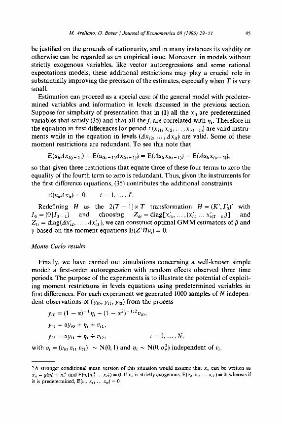
be justified on the grounds of stationarity, and in many instances its validity or otherwise can be regarded as an empirical issue. Moreover, in models without strictly exogenous variables, like vector autoregressions and some rational expectations models, these additional restrictions may play a crucial role in substantially improving the precision of the estimates, especially when T is very small.

Estimation can proceed as a special case of the general model with predetermined variables and information in levels discussed in the previous section. Suppose for simplicity of presentation that in (1) all the xit are predetermined variables that satisfy (35) and that all theJ; are correlated with ?i. Therefore in the equation in first differences for period t (Xii, Xi2, . . . , Xi(t_ 1J are valid instruments while in the equation in levels (dxiz, . . , Axit) are valid. Some of these moment restrictions are redundant. To see this note that

E(tWtxi(,- 1)) - E(uic,-i+txi(,- 1)) = E(dui,xi(,- 1)) - E(dU:,xi(,-2)),

so that given three restrictions that equate three of these four terms to zero the equality of the fourth term to zero is redundant. Thus, given the instruments for the first difference equations, (35) contributes the additional constraints

E(uitdXi,) = 0, t= l,...,T.

Redefining Z-Z as the 2(T - 1) x T transformation H = (K’,Zb)’ with I0 = (OlZ,_,) and choosing Zdi = diag[xf,, . . . ,(x;, . . . XI{=_ I,)] and ZIi = diag(dx,$, . . , dxlT), we can construct optimal GMM estimators of /I and y based on the moment equations E(Z’Hui) = 0.

Monte Carlo results

Finally, we have carried out simulations concerning a well-known simple model: a first-order autoregression with random effects observed three time periods. The purpose of the experiments is to illustrate the potential of exploiting moment restrictions in levels equations using predetermined variables in first differences. For each experiment we generated 1000 samples of N independent observations of (yio, yii, yiz) from the process

yi, = (1 - tl)-lyli + (1 - a2)-1’20i~,

Yil = aYi0 + ‘li + uil7

Yi2 = @Yil + ?i + ui27 i=l N, ? ... 7

with Ui = (uio Vi1 Viz)’ N N(0, I) and V]i - N(0, 0,‘) independent of Vi.

5A stronger conditional mean version of this situation would assume that x,, can be written as

x,~ = g(qi) + xi: and E(qi 1 xi: x$) = 0. If xi, is strictly exogenous, E(vi,I xi1 xIT) = 0, whereas if

it is predetermined, E(vi, 1 xi1 xi,) = 0.


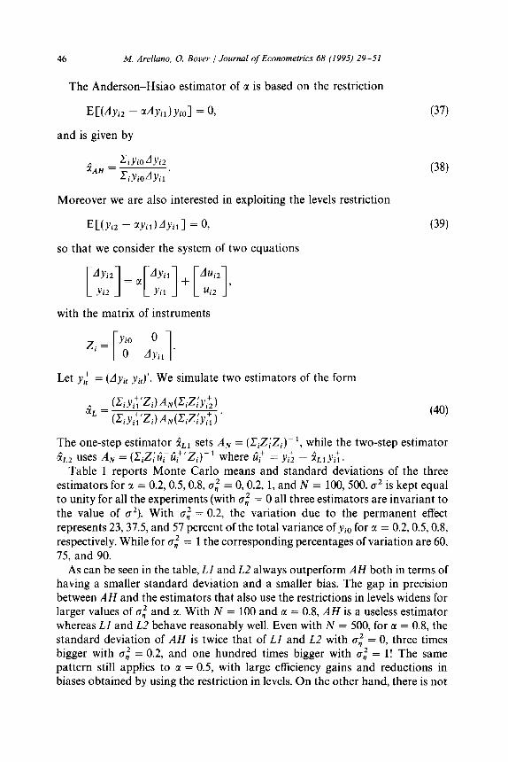
The Anderson-Hsiao estimator of a is based on the restriction

and is given by

. CiYi,AJ1i2 UAH = ZiYioAYil’

Moreover we are also interested in exploiting the levels restriction

so that we consider the system of two equations

with the matrix of instruments

Zi = ‘~ [ 1 A~, .

11

Let yl = (Ayi, yi,)‘. We simulate two estimators of the form

(37)

(38)

(39)

(40)

The one-step estimator gL1 sets AN = (CiZfZi)) ‘, while the two-step estimator BL2 uses AN = (CiZlu^+u^+‘Zi)- ’ where I&+ = y; - &LryA.

Table 1 reports Monte Carlo means and standard deviations of the three estimators for 0: = 0.2,0.5,0.&o,” = 0,0.2, 1, and N = 100, 500. rr2 is kept equal to unity for all the experiments (with 0,’ = 0 all three estimators are invariant to the value of a’). With rr,’ = 0.2, the variation due to the permanent effect represents 23,37.5, and 57 percent of the total variance Of yi, for a = 0.2,0.5,0.8, respectively. While for CI~ = 1 the corresponding percentages of variation are 60,

75, and 90. As can be seen in the table, LI and L2 always outperform AH both in terms of

having a smaller standard deviation and a smaller bias. The gap in precision between AH and the estimators that also use the restrictions in levels widens for larger values of 0,” and CI. With N = 100 and M = 0.8, AH is a useless estimator whereas LI and L2 behave reasonably well. Even with N = 500, for u = 0.8, the standard deviation of AH is twice that of Ll and L2 with 0,’ = 0, three times bigger with 0,’ = 0.2, and one hundred times bigger with D: = l! The same pattern still applies to CI = 0.5, with large efficiency gains and reductions in biases obtained by using the restriction in levels. On the other hand, there is not

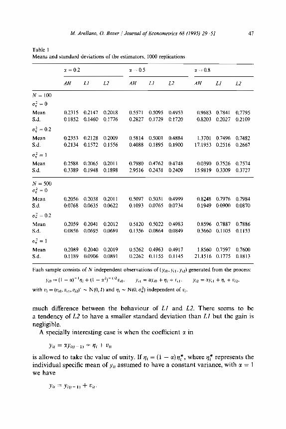
M. Arellano, 0. Bover / Journal of Econometrics 68 (1995) 29-51 47

Table 1 Means and standard deviations of the estimators, 1000 replications

c( = 0.2 G( =0.5 a =0.8

AH Li LZ AH Ll L2 AH LI L2

N=lOO

0; = 0

Mean 0.2315 0.2147 0.2018 0.5571 0.5095 0.4953 0.9683 0.7841 0.7795

S.d. 0.1852 0.1460 0.1776 0.2827 0.1729 0.1720 0.8203 0.2027 0.2109

u; = 0.2

Mean 0.2353 0.2128 0.2009 0.5814 0.5001 0.4884 1.3701 0.7496 0.7482

S.d. 0.2134 0.1572 0.1556 0.4088 0.1895 0.1900 17.1953 0.2516 0.2667

cl; = I

Mean 0.2588 0.2065 0.2011 0.7980 0.4762 0.4748 0.0390 0.7526 0.7574

S.d. 0.3389 0.1948 0.1898 2.9516 0.2431 0.2409 15.9819 0.3309 0.3727

N = 500

0,‘=0

Mean 0.2056 0.2038 0.2011 0.5097 0.503 I 0.4999 0.8248 0.7976 0.7984

Sd. 0.0768 0.0635 0.0622 0.1093 0.0765 0.0734 0.1949 0.0900 0.0870

u; = 0.2

Mean 0.2059 0.2041 0.2012 0.5 120 0.5022 0.4983 0.8596 0.7887 0.7886

S.d. 0.0856 0.0695 0.0689 0.1356 0.0864 0.0849 0.3660 0.1105 0.1153

uf = 1

Mean 0.2089 0.2040 0.2019 0.5262 0.4963 0.4917 1.8560 0.7597 0.7600

S.d. 0.1189 0.0906 0.0891 0.2262 0.1155 0.1145 21.1516 0.1775 0.1813

Each sample consists of N independent observations of (Y,~, yi, , yJ generated from the process:

yio = (1 - cc)-‘qi + (1 - cz~)-“%io, y,, = G(yilJ + vi + V,l, yi2 = XY,l + rl, + vi23

with vi = (v,~, uilr viz)’ - N(0, I) and vi - N(0, u,‘) independent of vi.

much difference between the behaviour of Ll and L2. There seems to be a tendency of L2 to have a smaller standard deviation than LI but the gain is

negligible. A specially interesting case is when the coefficient c1 in

Yit = aYi(t- 1) + Vi + uir

is allowed to take the value of unity. If vi = (1 - a) q*, where qT represents the individual specific mean of yi, assumed to have a constant variance, with M = 1 we have

Yit = Yi(t- 1) + uit.

48 M. AreNano, 0. Bover /Journal of Econometrics 68 (1995) 29-51

The alternative specification of the model with c( = 1 would be a random walk with an individual drift Y]i. In the former case, with a = 1, E(yiodyi,) = 0 and as a consequence the Anderson-Hsiao restriction (37) fails to identify a. However, the level restriction (39) still applies and could be exploited in order to test the stationary autoregressive model against the random walk model without drift.

5. Conclusions

Models with predetermined variables for panel data are typically estimated in first differences using instruments in levels. In these models, the absence of information about the parameters of interest in the levels of the variables results in the loss of what sometimes is a very substantial part of the total variation in the data. In this article, we are concerned with panel data models that specify valid instruments for the equations in levels, in addition to those available for the equations in first differences or deviations from individual means. Static models of this kind, but using exclusively strictly exogenous explanatory variables, were first considered by Hausman and Taylor (1981) and, with the addition of a lagged dependent variable, by Bhargava and Sargan (1983). The impact of these models in applied work has been limited, partly due to the difficulty in finding exogenous variables that can be convincingly regarded a priori as being uncorrelated with the individual effects, and partly due to the difficulty in finding strictly exogenous variables at all.

This paper considers models with predetermined instrumental variables that are uncorrelated with the effects. The particular type of variables of this kind that we emphasize are first differences of predetermined variables that have a constant correlation with the effects. A similar assumption for strictly exogenous variables was previously exploited by Bhargava and Sargan (1983) and Breusch, Mizon, and Schmidt (1989). Thus, in addition to using instruments in levels for equations in first differences, we propose to use instruments in first differences for equations in levels. The potential gains in precision from using these constraints are illustrated by means of simulations of alternative estimators of an autoregressive model. Moreover, we also explain how the assumption of constant correlation with the effects can be exploited to test for unit roots in short panels against a stationary autoregressive model.

The paper presents a GMM formulation of Hausman-Taylor (HT) and related estimators with unrestricted covariance matrix, together with a derivation of the information bound for these models. We use this framework to extend HT-type estimators to models with predetermined variables. In doing this we unify a large literature in a coherent way. We propose a GMM estimator for a general model that includes time-invariant, strictly exogenous, and predetermined variables, a subset of which are uncorrelated with the effects. We also show that optimal estimators are invariant to the transformation used to

M. Arellano. 0. Bover / Journal of Econometrics 68 (1995) 29-51 49

remove the effects. Finally, we propose a new transformation, forward orthogonal deviations, which is a computationally convenient alternative for models with predetermined variables since it preserves the orthogonality among the errors.

Appendix

A. 1. GMM formulation of HT, AM, and BMS estimators

Let

W+=HWi= KWi

[ 1

zdi O w;

and Zi = [ 1 0 m(’

so that

Wi+‘Zi = ( WIK’Zdi ItCimi).

Now using that Kz = 0 we have KWi = (KXijO) and with 52 = a2Zr + ain’,

,Q+ =HQH’= .;I,‘) (K’ T -‘I) = o2 KK’ 0

0 1 (PT)-’ .

Therefore

ZIO+Zi = ~2 Z;iKK’Zdi 0

0 1 (82T)-1mimf ’ and

w’R’z(z’Rfi2R’z)-‘z’Rw

= ~iWi+‘Zi(CiZ1~+Zi)-‘CiZ! W+

1 Md [[ 0 0 =- fJ2 0 1 + e2TCiwim!(Cimim!)-‘Cimiwl 1 , (A.11

where

Md = CiXIK’Zdi (CiZ;iKK’Zdi)-‘CiZ~iK’Xi.

NOW with Zdi = IT- 1 Q w(, Md equals

(A.9

Md = sYiXf(I, @ Wi) [K’(KK’)-‘K @ (CiWiWi)-‘] Ci(ZT 0 Wi)Xi.

Moreover, since K’(KK’)- ‘K = Q = A’A, where A is the orthogonal deviations operator defined in Section 3, and the columns of AXi are linear combinations of

50 M. Arellano, 0. Bover 1 Journal of Econometrics 68 (1995) 29-51

the columns of Zdi, Md becomes

Md = CiXlA’Zdi(~iZl;iZdi)-’ CiZ;iAXi = CiXIA’AXi,

so that (A.1) equals

(l/a’) (ciwiQwi + 82TCiwimf (Cimimr)-’ Cimiwi’).

The derivation of the second term of (8) follows along the same lines. Note that this result only requires that the columns of AXi are linear

combinations of the columns of Zdi provided Zdi has the Kronecker structure. Thus, the estimators of the form given in (5) that use 6 remain unaltered if instead of Zdi = I @ wf we use

Zdi = I @ [VCC(KXt)]‘.

In addition, if we choose K = A, the block-diagonal specification of Zdi could be replaced by simply AXi without changing the estimator, as apparent from expression (A.2).

A.2. The information bound for Hausman-Taylor models

The model specifies the conditional moment restrictions

E(ui( Wii) = 0 and E(Kuil Wii, wzi) = 0.

Let us introduce the notation

pzi = K(yi - Wi6) = Kui,

where pji = pj(yi, Wi, 6), j = 1,2. Following Chamberlain (1992b) we consider a forward transformation of pii of the form

Pli = Pli - r(wi)P2ir

which given sequential conditioning ensures that E(p:il wii) = 0. We wish to choose T(wi) such that E(pfip;i 1 wi) = 0. Since

E(pfip;ilwi) = QiK’ - I’(Wi) KQiK’,

the condition is satisfied if

T(Wi) = S2iK’(KS2iK’)-‘,

where 521 = s2(Wi). Thus

p:i = Ui - SZiK’(KS2iK’)-‘Kui = ~(l’a;‘1)-l 1’52,~‘~i.

M. Arellano, 0. Bover / Journal of Economehics 68 (1995) 29-5 I 51

Therefore, the bound for 6 will be the sum of the bounds corresponding to each of the conditional moments

E(Kui 1 Wi) = 0,

E[(Z’S);‘1)-‘Z’a;‘UiI Wli] ~0.

References

Ahn, S. and P. Schmidt, 1995, Efficient estimation of models for dynamic panel data, this issue.

Amemiya, T. and T.E. MaCurdy, 1986, Instrumental-variable estimation of an error-components

model, Econometrica 54, 869-881.

Anderson, T.W. and C. Hsiao, 1982, Formulation and estimation of dynamic models using panel

data, Journal of Econometrics 18, 47-82.

Arellano, M. and S.R. Bond, 1991, Some tests of specification for panel data: Monte Carlo evidence

and an application to employment equations, Review of Economic Studies 58, 2777297.

Balestra, P. and M. Nerlove, 1966, Pooling cross section and time series data in the estimation of

a dynamic model: The demand for natural gas, Econometrica 34, 5855612.

Bhargava, A. and J.D. Sargan, 1983, Estimating dynamic random effects models from panel data

covering short time periods, Econometrica 51, 163551659.

Breusch, T.S.. G.E. Mizon, and P. Schmidt, 1989, Efficient estimation using panel data, Econo-

metrica 57, 695-700.

Chamberlain, G., 1982, Multivariate regression models for panel data, Journal of Econometrics 18,

5-46.

Chamberlain, G., 1984, Panel data, in: Z. Griliches and M.D. Intriligator, eds., Handbook of

econometrics, Vol. 2 (Elsevier, Amsterdam) 124771313.

Chamberlain. G., 1987, Asymptotic efficiency in estimation with conditional moment restrictions,

Journal of Econometrics 34, 305-334.

Chamberlain, G., 1992a, Efficiency bounds for semiparametric regression, Econometrica 60.

567-596.

Chamberlain, G., 1992b, Comment: Sequential moment restrictions in panel data, Journal of

Business and Economic Statistics 10, 20-26.

Hansen, L.P., 1982, Large sample properties of generalized method of moments estimators. Econo-

metrica 50. 102991054.

Hausman, J.A. and W.E. Taylor, 1981, Panel data and unobservable individual effects, Econo-

metrica 49, 1377- 1398.

Hayashi, F. and C. Sims, 1983, Nearly efficient estimation of time series models with predetermined,

but not exogenous, instruments, Econometrica 51, 783-798.

Holtz-Eakin, D., W. Newey, and H. Rosen, 1988. Estimating vector autoregressions with panel data,

Econometrica 56, 1371-1395.

Schmidt, P., S.C. Ahn, and D. Wyhowski, 1992, Comment, Journal of Business and Economic

Statistics 10, 10-14.

White. H., 1982, Instrumental variables regression with independent observations, Econometrica 50,

483-499.

of econometrics - cemfiarellano/arellano-bover-1995.pdf · a closely related transformation has...

Documents