ocean scale hypoxia-based habitat compression of atlantic

Ocean scale hypoxia-based habitat compression of Atlanticistiophorid billfishes

ERIC D. PRINCE,1,* JIANGANG LUO,2

C. PHILLIP GOODYEAR,3 JOHN P.HOOLIHAN,1 DERKE SNODGRASS,1 ERIC S.ORBESEN,1 JOSEPH E. SERAFY,1 MAURICIOORTIZ1 AND MICHAEL J. SCHIRRIPA1

1National Marine Fisheries Service, Southeast Fisheries ScienceCenter, 75 Virginia Beach Drive, Miami, FL 33149, USA2Rosenstiel School of Marine and Atmospheric Science,University of Miami, 4600 Rickenbacker Causeway, Miami, FL

33149, USA31214 North Lakeshore Drive, Niceville, FL 32578, USA

ABSTRACT

Oxygen minimum zones (OMZs) below near-surfaceoptimums in the eastern tropical seas are among thelargest contiguous areas of naturally occurring hypoxiain the world oceans, and are predicted to expand andshoal with global warming. In the eastern tropicalPacific (ETP), the surface mixed layer is defined by ashallow thermocline above a barrier of cold hypoxicwater, where dissolved oxygen levels are £3.5 mL L)1.This thermocline (�25–50 m) constitutes a lowerhypoxic habitat boundary for high oxygen demandtropical pelagic billfish and tunas (i.e., habitat com-pression). To evaluate similar oceanographic condi-tions found in the eastern tropical Atlantic (ETA), wecompared vertical habitat use of 32 sailfish (Istiophorusplatypterus) and 47 blue marlin (Makaira nigricans)monitored with pop-up satellite archival tags in theETA and western North Atlantic (WNA). Both spe-cies spent significantly greater proportions of theirtime in near-surface waters when inside the ETA thanwhen in the WNA. We contend that the near-surfacedensity of billfish and tunas increases as a consequenceof the ETA OMZ, therefore increasing their vulnera-bility to overexploitation by surface gears. Because theETA OMZ encompasses nearly all Atlantic equatorialwaters, the potential impacts of overexploitation are aconcern. Considering the obvious differences in

catchability inside and outside the compression zones,it seems essential to standardize these catch ratesseparately to minimize inaccuracies in stock assess-ments for these species. This is especially true in lightof global warming, which will likely exacerbate futurecompression impacts.

Key words: Atlantic hypoxia-based habitat com-pression, climate change, global warming, oxygenminimum zones, tropical pelagic fishes

INTRODUCTION

Spatial and temporal fluctuations of environmentalconditions in the world’s oceans influence the verticaland horizontal movement of pelagic fishes (Sharp,1978; Fonteneau, 1997; Prince and Goodyear, 2006;Bigelow and Maunder, 2007). Adequate populationestimates of pelagic fishes are often conditioned onspatial distribution assumptions made during the stockassessment process (Brill, 1994; Brill and Lutcavage,2001). Increasingly, habitat use preferences and asso-ciated physiological limits of pelagic species are usedto evaluate their influences on catch per unit effort(CPUE) (Hanamoto, 1987; Hinton and Nakano,1996; Fonteneau, 1997; Goodyear, 2003; Maunderet al., 2006; Bigelow and Maunder, 2007). Makingadjustments for these influences (i.e., CPUE stan-dardization) is essential when using catch rates asindices of relative abundance to infer population stockstatus (Goodyear, 2003; Hinton and Maunder, 2004).Brill and Lutcavage (2001) expressed a similar view-point and maintained that understanding environ-mental influences on movements and depthdistributions of tunas and billfishes is important forimproving population assessments. In fact, failure toincorporate environmental influences on the distri-bution of fishes in the standardization process mayresult in biased estimates of population bench marks(Bigelow and Maunder, 2007), potentially leading todifferent stock status perceptions (ICCAT, 2004).

Oxygen minimum zones (OMZs) below near-surface optimums in the eastern tropical seas areamong the largest contiguous areas of naturallyoccurring hypoxia in the world oceans (Bakun, 1996;

*Correspondence. e-mail: [email protected]

Received 29 January 2010

Revised version accepted 19 July 2010

FISHERIES OCEANOGRAPHY Fish. Oceanogr. 19:6, 448–462, 2010

448 doi:10.1111/j.1365-2419.2010.00556.x Published 2010. This article is a US Government work

and is in the public domain in the USA

Diaz, 2001; Stramma et al., 2008). Development ofOMZs is primarily a function of prevailing weatherpatterns and oceanographic ⁄ biological processes.These include winds that parallel the coastline off thewest coasts of continents, leading to intense nutrientupwelling, the advection process, the absence of sig-nificant mixing at depth, stagnant deep water layers,and the extremely productive surface mixed layer thatresults in a continuous rain of biological material thatdeteriorates while sinking into the upwelling watermass (Cushing, 1969; Bakun, 1996; Bakun et al.,1999). All these processes contribute to a narrowsurface layer with uniform temperature, shallowthermocline with a steep gradient, and a hypoxicenvironment below the thermocline, which togethercharacterizes the more or less permanent OMZs (Diaz,2001; Helly and Levin, 2004).

Hypoxia-based habitat compression, associatedwith OMZs, has been reported for a variety of marineteleosts, including estuarine and coastal species (Ebyand Crowder, 2002), demersal reef fishes in the Gulf ofMexico (Stanley and Wilson, 2004), and many otherpelagic and demersal species (see review by Ekau et al.,2009). For example, Ingham et al. (1977) reportedthat surface sightings of schooling skipjack tuna(Katsuwonus pelamis) in the eastern Atlantic weregreater in areas where the oxycline was shallow. Evanset al. (1981) explored this further by comparing catchdata with environmental indicators (i.e., temperatureand dissolved oxygen) to infer habitat limits and vul-nerability to surface fishing gears for skipjack tuna inthe equatorial eastern and western Atlantic.

Recently, Prince and Goodyear (2006) presentedthe first empirical data, based on direct measurementof vertical movement, which showed that OMZs re-strict the depth distribution of tropical pelagic bluemarlin (Makaira nigricans) and sailfish (Istiophorusplatypterus) in the eastern tropical Pacific (ETP), pre-sumably by compressing their suitable physical habitatinto a narrow surface layer. In this case, the surfacemixed layer extended downward to a variable bound-ary defined by a shallow thermocline, often around 25–50 m, above a barrier of cold hypoxic water (Princeand Goodyear, 2006). While hypoxia-based habitatcompression is evident in the ETP for tropical pelagicfishes, it is not present in the western North Atlantic(WNA), where dissolved oxygen (DO) is not limitedat increasing depths (Prince and Goodyear, 2006).Interestingly, the oceanographic features in the east-ern tropical Atlantic (ETA) are similar to those in theETP; however, empirical evidence of hypoxia-basedhabitat compression for tropical pelagic fishes in theETA has not yet been reported.

Dissolved oxygen is an important parameter forunderstanding the role of oceans in climate change(Stramma et al., 2008). In the current cycle of climatechange involving escalated global warming and oceanacidification (ocean absorption of anthropogenic CO2

emissions), oxygen minimum zones in the tropicaloceans are predicted to increase in surface extent, totalvolume and severity while shoaling closer to the seasurface (Bograd et al., 2008; Rosa and Seibel, 2008;Stramma et al., 2008, 2009). Rosa and Seibel (2008)predicted that the synergism between ocean acidifi-cation, global warming, and expansion of OMZs willfurther reduce the habitat available to major oceanicpredators. Clearly, the trophic cascading impacts ofthese processes and the resultant habitat compressionon pelagic and demersal biota need to be determinedfor the major aquatic communities within eachaffected area.

Objectives of this paper were: (i) to examine theeffect of hypoxia-based habitat compression in theETA by evaluating empirical data on vertical habitatuse of eastern and western Atlantic blue marlin andsailfish using pop-up satellite archival tag (PSAT)technology; and (ii) to describe the unique oceano-graphic features in the Atlantic oxygen minimumzones that contribute to habitat compression and theirrelevance to management of pelagic resources.

METHODS

Tag sampling design to monitor habitat of Istiophoridae

We followed the PSAT rigging procedures describedby Prince and Goodyear (2006) and Goodyear et al.(2008). Billfish handling, in-water tagging procedures,and tagging devices reviewed by Prince et al. (2002)were also used. PSATs were attached about 4–5 cmbelow the dorsal midline by inserting a double-barbedmedical-grade nylon anchor between the pterygio-phores to a depth just short of protruding from theopposite side of the fish. A conventional streamer tagwas also inserted posterior of the PSAT (Prince et al.,2002).

PSATs were programmed for deployment durationsranging from 7 to 120 days. Programming protocols forPSATs are detailed in Prince and Goodyear (2006)and Goodyear et al. (2008).

We deployed 79 PSATs on blue marlin and sailfishfrom 2001 to 2006, primarily from recreational fishingvessels, in both the western and eastern tropical-sub-tropical Atlantic basins using standard trolling gearwith natural bait or high-speed lures (Table 1). AllPSAT deployment activities were conducted within

Hypoxia-based habitat compression of billfishes 449

Published 2010. This article is a US Government work and is in the public domain in the USA, Fish. Oceanogr., 19:6, 448–462.

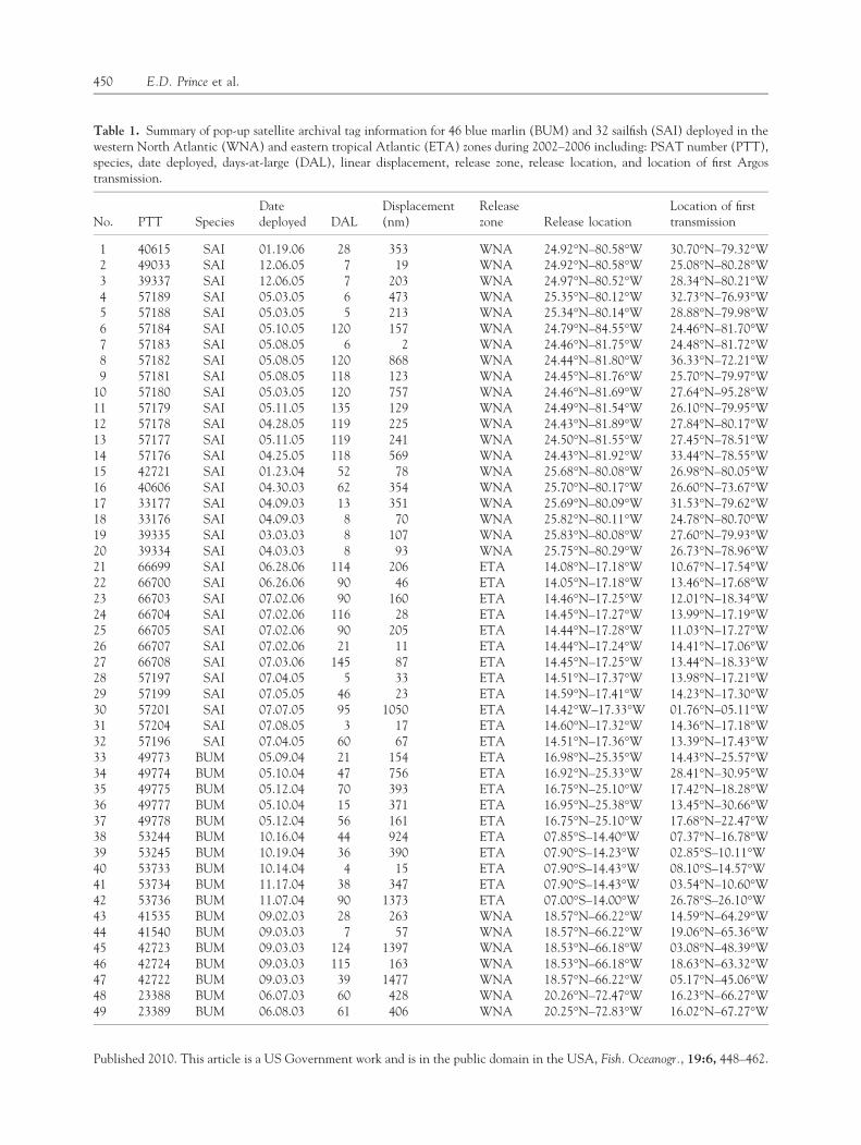
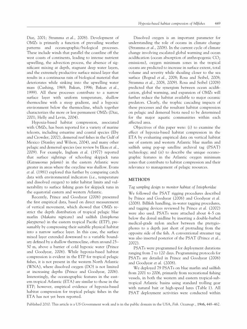
Table 1. Summary of pop-up satellite archival tag information for 46 blue marlin (BUM) and 32 sailfish (SAI) deployed in thewestern North Atlantic (WNA) and eastern tropical Atlantic (ETA) zones during 2002–2006 including: PSAT number (PTT),species, date deployed, days-at-large (DAL), linear displacement, release zone, release location, and location of first Argostransmission.

No. PTT SpeciesDatedeployed DAL

Displacement(nm)

Releasezone Release location

Location of firsttransmission

1 40615 SAI 01.19.06 28 353 WNA 24.92�N–80.58�W 30.70�N–79.32�W2 49033 SAI 12.06.05 7 19 WNA 24.92�N–80.58�W 25.08�N–80.28�W3 39337 SAI 12.06.05 7 203 WNA 24.97�N–80.52�W 28.34�N–80.21�W4 57189 SAI 05.03.05 6 473 WNA 25.35�N–80.12�W 32.73�N–76.93�W5 57188 SAI 05.03.05 5 213 WNA 25.34�N–80.14�W 28.88�N–79.98�W6 57184 SAI 05.10.05 120 157 WNA 24.79�N–84.55�W 24.46�N–81.70�W7 57183 SAI 05.08.05 6 2 WNA 24.46�N–81.75�W 24.48�N–81.72�W8 57182 SAI 05.08.05 120 868 WNA 24.44�N–81.80�W 36.33�N–72.21�W9 57181 SAI 05.08.05 118 123 WNA 24.45�N–81.76�W 25.70�N–79.97�W

10 57180 SAI 05.03.05 120 757 WNA 24.46�N–81.69�W 27.64�N–95.28�W11 57179 SAI 05.11.05 135 129 WNA 24.49�N–81.54�W 26.10�N–79.95�W12 57178 SAI 04.28.05 119 225 WNA 24.43�N–81.89�W 27.84�N–80.17�W13 57177 SAI 05.11.05 119 241 WNA 24.50�N–81.55�W 27.45�N–78.51�W14 57176 SAI 04.25.05 118 569 WNA 24.43�N–81.92�W 33.44�N–78.55�W15 42721 SAI 01.23.04 52 78 WNA 25.68�N–80.08�W 26.98�N–80.05�W16 40606 SAI 04.30.03 62 354 WNA 25.70�N–80.17�W 26.60�N–73.67�W17 33177 SAI 04.09.03 13 351 WNA 25.69�N–80.09�W 31.53�N–79.62�W18 33176 SAI 04.09.03 8 70 WNA 25.82�N–80.11�W 24.78�N–80.70�W19 39335 SAI 03.03.03 8 107 WNA 25.83�N–80.08�W 27.60�N–79.93�W20 39334 SAI 04.03.03 8 93 WNA 25.75�N–80.29�W 26.73�N–78.96�W21 66699 SAI 06.28.06 114 206 ETA 14.08�N–17.18�W 10.67�N–17.54�W22 66700 SAI 06.26.06 90 46 ETA 14.05�N–17.18�W 13.46�N–17.68�W23 66703 SAI 07.02.06 90 160 ETA 14.46�N–17.25�W 12.01�N–18.34�W24 66704 SAI 07.02.06 116 28 ETA 14.45�N–17.27�W 13.99�N–17.19�W25 66705 SAI 07.02.06 90 205 ETA 14.44�N–17.28�W 11.03�N–17.27�W26 66707 SAI 07.02.06 21 11 ETA 14.44�N–17.24�W 14.41�N–17.06�W27 66708 SAI 07.03.06 145 87 ETA 14.45�N–17.25�W 13.44�N–18.33�W28 57197 SAI 07.04.05 5 33 ETA 14.51�N–17.37�W 13.98�N–17.21�W29 57199 SAI 07.05.05 46 23 ETA 14.59�N–17.41�W 14.23�N–17.30�W30 57201 SAI 07.07.05 95 1050 ETA 14.42�W–17.33�W 01.76�N–05.11�W31 57204 SAI 07.08.05 3 17 ETA 14.60�N–17.32�W 14.36�N–17.18�W32 57196 SAI 07.04.05 60 67 ETA 14.51�N–17.36�W 13.39�N–17.43�W33 49773 BUM 05.09.04 21 154 ETA 16.98�N–25.35�W 14.43�N–25.57�W34 49774 BUM 05.10.04 47 756 ETA 16.92�N–25.33�W 28.41�N–30.95�W35 49775 BUM 05.12.04 70 393 ETA 16.75�N–25.10�W 17.42�N–18.28�W36 49777 BUM 05.10.04 15 371 ETA 16.95�N–25.38�W 13.45�N–30.66�W37 49778 BUM 05.12.04 56 161 ETA 16.75�N–25.10�W 17.68�N–22.47�W38 53244 BUM 10.16.04 44 924 ETA 07.85�S–14.40�W 07.37�N–16.78�W39 53245 BUM 10.19.04 36 390 ETA 07.90�S–14.23�W 02.85�S–10.11�W40 53733 BUM 10.14.04 4 15 ETA 07.90�S–14.43�W 08.10�S–14.57�W41 53734 BUM 11.17.04 38 347 ETA 07.90�S–14.43�W 03.54�N–10.60�W42 53736 BUM 11.07.04 90 1373 ETA 07.00�S–14.00�W 26.78�S–26.10�W43 41535 BUM 09.02.03 28 263 WNA 18.57�N–66.22�W 14.59�N–64.29�W44 41540 BUM 09.03.03 7 57 WNA 18.57�N–66.22�W 19.06�N–65.36�W45 42723 BUM 09.03.03 124 1397 WNA 18.53�N–66.18�W 03.08�N–48.39�W46 42724 BUM 09.03.03 115 163 WNA 18.53�N–66.18�W 18.63�N–63.32�W47 42722 BUM 09.03.03 39 1477 WNA 18.57�N–66.22�W 05.17�N–45.06�W48 23388 BUM 06.07.03 60 428 WNA 20.26�N–72.47�W 16.23�N–66.27�W49 23389 BUM 06.08.03 61 406 WNA 20.25�N–72.83�W 16.02�N–67.27�W

450 E.D. Prince et al.


50 miles of the coastlines off South Florida, theBahamas, Turks and Caicos Islands and U.S. VirginIslands in the WNA, and off Cape Verde Islands,Ascension Island, and Dakar, Senegal, in the ETA(Fig. 1). Wildlife Computers1 (Redmond, WA) PAT4and Mk10 were the primary PSAT models used,although a few PAT2 and PAT3 models were usedduring 2001–2003. The PSATs were programmed tosample depth (pressure), temperature and light onceevery 30 or 60 s. The depth and temperature recordsfor a few of the early deployments were summarized bythe software on-board the tag into histograms at 3-hintervals, but the vast majority of the data werecompiled by the on-board software into histograms at

6-h bin intervals. We programmed the tag to sum-marize temperature bins starting at <12�C, then eachsuccessive 2�C interval ending with >32�C. Likewise,depth bins started at <)1 m, then successive intervalsof 25 m until ending at depths >250 m. The aggregatemean proportions for monitoring time and recordswith one or more dives (to the maximum depth re-corded in a record) were calculated within <50, >50,>100, and >200-m depth strata, then compared amongspecies ⁄ area treatments.

Statistical analysis of vertical habitat use

General linear model (GLM) univariate procedures inSPSS software (Chicago, IL, USA) were used tocompare group mean proportions (arcsine transformeddata) for aggregate time spent at-depth and maximumdive records between the ETA and WNA. Maximumdive records were extracted from individual 6-h sum-mary bins. For analytical purposes, data were assigned

Table 1. (Continued).

No. PTT SpeciesDatedeployed DAL

Displacement(nm)

Releasezone Release location

Location of firsttransmission

50 23397 BUM 06.09.03 38 80 WNA 20.30�N–72.62�W 18.98�N–72.85�W51 41537 BUM 07.24.03 45 498 WNA 32.13�N–65.01�W 36.11�N–56.20�W52 41527 BUM 07.14.03 41 203 WNA 32.05�N–65.03�W 34.78�N–67.43�W53 41516 BUM 06.11.03 57 212 WNA 24.05�N–75.43�W 27.25�N–73.78�W54 41518 BUM 06.05.03 63 492 WNA 24.33�N–72.53�W 31.20�N–77.59�W55 41520 BUM 06.05.03 63 825 WNA 24.10�N–75.25�W 36.85�N–69.23�W56 41521 BUM 06.07.03 61 176 WNA 24.10�N–75.25�W 22.25�N–72.77�W57 41522 BUM 06.09.03 10 80 WNA 24.08�N–75.25�W 24.98�N–74.17�W58 41523 BUM 06.04.03 95 218 WNA 24.10�N–75.25�W 24.55�N–71.29�W59 41524 BUM 06.04.03 82 319 WNA 24.10�N–75.28�W 19.03�N–73.56�W60 41525 BUM 06.07.03 41 342 WNA 24.12�N–75.27�W 29.79�N–75.85�W61 41526 BUM 06.07.03 84 699 WNA 24.12�N–75.30�W 35.70�N–73.83�W62 41528 BUM 06.10.03 69 255 WNA 24.11�N–75.28�W 28.26�N–74.28�W63 41530 BUM 06.26.03 7 91 WNA 22.85�N–74.41�W 24.36�N–74.42�W64 41531 BUM 06.19.03 91 199 WNA 22.00�N–72.06�W 23.93�N–69.12�W65 41534 BUM 06.17.03 46 549 WNA 22.00�N–72.07�W 19.13�N–62.78�W66 41538 BUM 06.16.03 47 1125 WNA 21.99�N–72.03�W 14.29�N–54.01�W67 41539 BUM 06.18.03 74 92 WNA 21.99�N–72.06�W 20.62�N–71.31�W68 25999 BUM 06.14.02 45 747 WNA 23.93�N–74.59�W 17.41�N–63.24�W69 22872 BUM 06.14.02 28 353 WNA 23.94�N–74.61�W 25.00�N–68.26�W70 23077 BUM 06.21.02 19 71 WNA 23.79�N–74.36�W 24.93�N–74.70�W71 26001 BUM 07.08.02 25 795 WNA 22.78�N–74.39�W 35.51�N–70.16�W72 26005 BUM 07.06.02 13 72 WNA 22.82�N–74.38�W 22.70�N–75.68�W73 23520 BUM 07.02.02 25 245 WNA 22.80�N–74.35�W 26.79�N–73.41�W74 27825 BUM 10.12.02 29 566 WNA 18.71�N–64.82�W 15.56�N–74.13�W75 22870 BUM 06.09.02 36 499 WNA 28.71�N–78.89�W 36.27�N–74.76�W76 23548 BUM 06.11.02 33 490 WNA 28.76�N–78.79�W 35.99�N–74.37�W77 26935 BUM 10.12.02 39 287 WNA 18.72�N–64.83�W 21.78�N–60.92�W78 23205 BUM 10.13.02 38 1193 WNA 18.72�N–64.82�W 07.54�N–47.90�W79 39334 BUM 10.14.02 43 229 WNA 18.85�N–64.79�W 22.44�N–66.18�W

1References to commercial products do not imply endorse-

ment by the National Marine Fisheries Service or the au-

thors.



to four arbitrary depth strata (0–50 m, 51–100 m,101–200 m, and >200 m). In the evaluation, area (i.e.,ETA or WNA) was used as a fixed variable, depth as arandom variable, and proportion of time at-depth (ormaximum dives) as the dependent variable. Light le-vel derived geolocations allowed estimation of dateswhen two blue marlin (PTT 49774 and 53736) taggedin the ETA OMZ moved outside this area. Data forthese two individuals were split to correspond with thetime and area of occupancy. Computations for meanmaximum dives per day and mean temperature forthese maximum dives both inside and outside ETAused the same statistical approach as the aggregateanalysis.

Oceanography of the study areas

We constructed distributions of temperature, DO, andsalinity at-depth profiles in the rectangles given by theco-ordinates of the PSAT deployment and pop-offlocations for each month at-large for individual fishpooled by ETA or WNA study areas. These compila-tions employed the objectively analyzed monthlymeans for each variable at 1� of latitude and longitudefrom the World Ocean Atlas 2005 (WOA05) (http://www.nodc.noaa.gov/OC5/WOA05/woa05data.html,

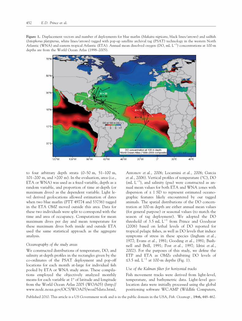
Antonov et al., 2006; Locarnini et al., 2006; Garciaet al., 2006). Vertical profiles of temperature (�C), DO(mL L)1), and salinity (psu) were constructed as an-nual mean values for both ETA and WNA zones withdispersion of ± 1 SD to represent estimated oceano-graphic features likely encountered by our taggedanimals. The spatial distributions of the DO concen-tration at 100-m depth are either annual mean values(for general purpose) or seasonal values (to match theseason of tag deployment). We adopted the DOthreshold of 3.5 mL L)1 from Prince and Goodyear(2006) based on lethal levels of DO reported fortropical pelagic fishes, as well as DO levels that inducesymptoms of stress in these species (Ingham et al.,1977; Evans et al., 1981; Gooding et al., 1981; Bush-nell and Brill, 1991; Post et al., 1997; Idrisi et al.,2002). For the purposes of this study, we define theETP and ETA as OMZs exhibiting DO levels of£3.5 mL L)1 at 100-m depths (Fig. 1).

Use of the Kalman filter for horizontal tracks

Fish movement tracks were derived from light-level,temperature, and bathymetric data. Light-level geo-location data were initially processed using the globalpositioning software WC-AMP (Wildlife Computers,

Figure 1. Displacement vectors and number of deployments for blue marlin (Makaira nigricans, black lines ⁄ arrows) and sailfish(Istiophorus platypterus, white lines ⁄ arrows) tagged with pop-up satellite archival tag (PSAT) technology in the western NorthAtlantic (WNA) and eastern tropical Atlantic (ETA). Annual mean dissolved oxygen (DO, mL L)1) concentrations at 100-mdepths are from the World Ocean Atlas (1998–2005).



Redmond, WA, USA), and then applying a sea-sur-face temperature-corrected Kalman filter (Nielsenet al., 2006) to the light level-derived locations. Thesesea surface temperature-corrected geolocations have areported accuracy of £111 km (Nielsen et al., 2006).Finally, we used a custom bathymetry filter to relocatethe points that were on land or in shallow water, basedon 2 · 2 min grid ETOP02 bathymetry data (Anon,2006) and the daily maximum depth from the PSAT(Hoolihan and Luo, 2007).

RESULTS

Vertical habitat use of billfishes

A total of 79 PSATs were deployed on blue marlin andsailfish in the WNA and ETA from 2001 to 2006(Fig. 1; Table 1). Blue marlin were monitored for anaggregate 410 days (10 PSATs) in the ETA and1283 days (36 PSATs) in the WNA, whereas sailfishwere monitored for an aggregate 932 days (12 PSATs)

in the ETA and 1161 days (20 PSATs) in the WNA(Table 1).

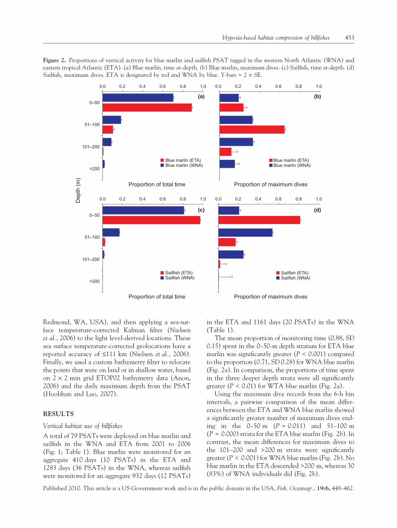
The mean proportion of monitoring time (0.88, SD0.15) spent in the 0–50-m depth stratum for ETA bluemarlin was significantly greater (P < 0.001) comparedto the proportion (0.71, SD 0.28) for WNA blue marlin(Fig. 2a). In comparison, the proportions of time spentin the three deeper depth strata were all significantlygreater (P < 0.01) for WTA blue marlin (Fig. 2a).

Using the maximum dive records from the 6-h binintervals, a pairwise comparison of the mean differ-ences between the ETA and WNA blue marlin showeda significantly greater number of maximum dives end-ing in the 0–50 m (P = 0.011) and 51–100 m(P = 0.000) strata for the ETA blue marlin (Fig. 2b). Incontrast, the mean differences for maximum dives tothe 101–200 and >200 m strata were significantlygreater (P < 0.001) for WNA blue marlin (Fig. 2b). Noblue marlin in the ETA descended >200 m, whereas 30(83%) of WNA individuals did (Fig. 2b).

(c)

(a) (b)

(d)

Figure 2. Proportions of vertical activity for blue marlin and sailfish PSAT tagged in the western North Atlantic (WNA) andeastern tropical Atlantic (ETA). (a) Blue marlin, time at-depth. (b) Blue marlin, maximum dives. (c) Sailfish, time at-depth. (d)Sailfish, maximum dives. ETA is designated by red and WNA by blue. Y-bars = 2 · SE.



The mean proportion of total time at-depth in the0–50 m stratum by sailfish in the ETA (0.97) wassignificantly greater (P < 0.001) than the WNA (0.81,Fig. 2c). In contrast, time at-depth in the 51–100 mstratum was significantly greater in the WNA (0.16),compared to the ETA (0.02, Fig. 2c). Time at-depthbelow this stratum was negligible, particularly for theETA group (Fig. 2c).

Sailfish in the ETA exhibited a significantly greater(P < 0.001) mean number of maximum dives endingin the 0–50 m stratum (Fig. 2d), whereas WNA sail-fish showed significantly higher means (P < 0.001) formaximum dives in the 51–100 and 101–200 m strata(Fig. 2d). Only one of 12 (8.3%) ETA sailfish des-cended >200 m, as compared to five of 20 (25%)WNA individuals.

Billfish movement across the WNA ⁄ ETA boundaries

During the study period, two blue marlin, PTT 49774and 53736 (Table 1), released in the ETA undertookmovements leading outside the OMZ (Figs 3a–c and4a–c). These marlin were at-large 47 days and 90 daysand had displacement distances of about 1400 and2543 km, respectively (Figs 3a and 4a). Kalman filtertracks of these marlin allowed estimation of the dateswhere transboundary movements between the ETAand waters outside this area were made, which in turnallowed analysis of vertical habitat use by the same fishinside and outside the OMZ (shown in red ⁄ black inFigs 3a–c and 4a–c). We compared maximum dailydepth records, and estimated temperature at thosedepths for PTT 49774 and 53736 (Figs 3a–c, and 4a–c), for activity inside and outside the ETA. For PTT49774, the mean daily maximum depth reached insidethe ETA was 91 m (SD 26) compared to 205 m (SD89) outside. Mean daily temperatures estimated atthese maximum depths inside the ETA were 21�C (SD2) compared to 21�C (SD 3) outside. For PTT 53736,the mean daily maximum depth reached inside theETA was 98 m (SD 51) compared to 189 m (SD 56)outside. The mean temperatures estimated at thesemaximum daily depths inside the ETA were 21�C (SD5) compared to 18�C (SD 3) outside. Both blue marlinexplored maximum daily depths and associated lowerwater temperatures outside the ETA that were signif-icantly greater (P < 0.000) than those inside the ETA.

Oceanographic conditions in the WNA and ETA

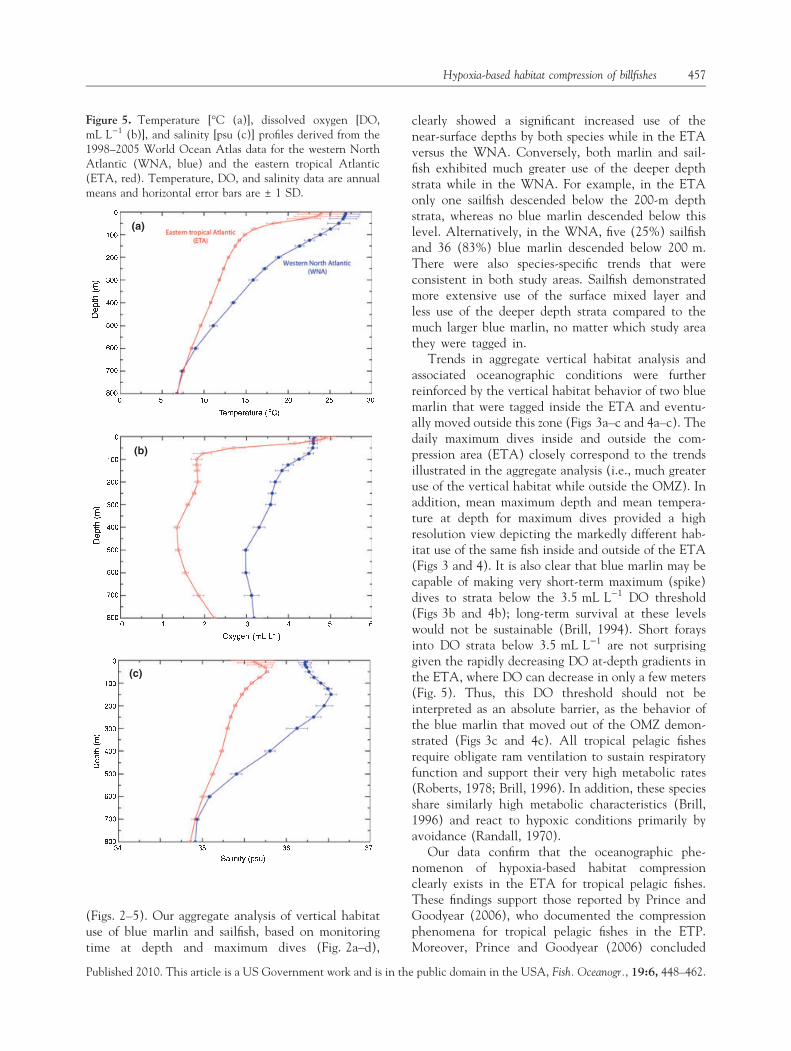
The temperature, DO, and salinity levels that ourtagged animals likely encountered in the two Atlanticstudy areas are shown in Fig. 5. Of these, the greatestdisparity between study areas was clearly the differ-ences in DO profiles (Fig. 5a). The DO concentrations

in the ETA were £3.5 mL L)1 below the thermocline(25–50-m depth strata), whereas in the WNA, DOlevels were maintained above this level through 400-mdepths, then tailed off gently to 3.2 mL L)1 through800-m depths. The DO gradient in the ETA was mostsevere between 10 and 50 m and then became moremoderate at depths below 75 m. There was a slight DOincrease in the ETA after 600 m through the deepestdepth strata shown (800 m), from 1.5 to 2.2 mL L)1,respectively. In the WNA, DO was above the3.5 mL L)1 threshold for the first 300 m, then variedbetween 3.2 and 3.5 mL L)1 thereafter. After the first10 m, DO in the WNA was always higher than theETA. Patterns for the temperature and salinity profilesfor the WNA and ETA were less pronounced, thoughsimilar, to the DO patterns (Fig. 5b,c).

DISCUSSION

For decades, OMZs have been reported to occur asdistinct strata in large equatorial regions of the easterntropical Pacific and Atlantic Oceans (Sund et al.,1981; Bakun, 1996; and Helly and Levin, 2004).While comparisons of skipjack tuna sightings andcatch data to environmental indicators (i.e., temper-ature and DO) have suggested vertical habitat com-pression within these OMZs (Evans et al., 1981), onlyrecently have empirical data (Prince and Goodyear,2006) demonstrated this phenomenon for high oxy-gen-demand blue marlin and sailfish (Post et al., 1997;Wegner et al., 2010). These data suggested that suit-able physical habitat of the ETP was compressed into anarrow surface mixed layer, and the cold hypoxicenvironment below the thermocline limited verticalhabitat use for tropical pelagic fishes (Prince andGoodyear, 2006).

Prince and Goodyear (2006) reported that thepreferred prey of marlin and sailfish (e.g., clupeids,carangids, small tunas), which are also obligate ramventilators, would be restricted to the same narrowsurface mixed layer. They suggested this would lead toincreased interaction between predator and prey,providing enhanced foraging opportunities for thepredators, thus attracting predators to these compres-sion zones. Historical data (1958–2005) from theInternational Commission for the Conservation ofAtlantic Tunas (ICCAT) and Inter-American Tropi-cal Tuna Commission (IATTC) indicate a largeraverage size for sailfish landed in the ETP and ETAcompared to the WNA [about 184 cm lower jaw forklength (LJFL) versus 164 cm LJFL, respectively],which may reflect these increased foraging opportu-nities (Prince and Goodyear, 2006).



The aggregate monitoring time achieved in thepresent study was well over 1 yr for each of thespecies ⁄ area treatments and are in general agreementwith findings reported for the ETP (Prince and

Goodyear, 2006). We have presented empirical dataon vertical habitat use of Atlantic istiophorid billfishand the associated oceanographic conditions theylikely encountered in the WNA versus ETA

(c)

(a)

(b)

Figure 3. (a) Kalman filter track (shownin white, see Methods) of a blue marlin(Makaira nigricans, PTT 49774) PSATdeployment initially released in the ETAthat made a transboundary movementoutside the ETA. The dates of trans-boundary crossing between study areas(28 May 2004) and the end point ofPSAT transmission (24 June 2004) areidentified. (b) Spring mean level of dis-solved oxygen at depth estimated fromthe World Ocean Atlas (1998–2005) formaximum dives (shown as blue line)during the track (PTT 49774). Percenttime at DO ⁄ maximum depth is propor-tional to the size of blue ovals. (c) Springmean temperature at depth estimatedfrom the World Ocean Atlas (1998–2005) for maximum dives during thetrack (49774). Percent time at tempera-ture ⁄ maximum depth is proportional tothe size of black ovals.



(c)

(a)

(b)

Figure 4. (a) Kalman filter track (shown in white, see Methods) of a blue marlin (Makaira nigricans, PTT 53736) PSATdeployment initially released in the ETA that made a transboundary movement outside the ETA. The dates of transboundarycrossing between study areas (21 December 2004) and the end point of PSAT transmission (5 February 2005) are identified. (b)Winter mean level of dissolved oxygen at depth estimated from the World Ocean Atlas (1998–2005) for maximum dives (shownas blue line) during the track (PTT 53736). Percent time at DO ⁄ maximum depth is proportional to the size of blue ovals. (c)Winter mean temperature at depth estimated from the World Ocean Atlas (1998–2005) for maximum dives during the track(53736). Percent time at temperature ⁄ maximum depth is proportional to the size of black ovals.



(Figs. 2–5). Our aggregate analysis of vertical habitatuse of blue marlin and sailfish, based on monitoringtime at depth and maximum dives (Fig. 2a–d),

clearly showed a significant increased use of thenear-surface depths by both species while in the ETAversus the WNA. Conversely, both marlin and sail-fish exhibited much greater use of the deeper depthstrata while in the WNA. For example, in the ETAonly one sailfish descended below the 200-m depthstrata, whereas no blue marlin descended below thislevel. Alternatively, in the WNA, five (25%) sailfishand 36 (83%) blue marlin descended below 200 m.There were also species-specific trends that wereconsistent in both study areas. Sailfish demonstratedmore extensive use of the surface mixed layer andless use of the deeper depth strata compared to themuch larger blue marlin, no matter which study areathey were tagged in.

Trends in aggregate vertical habitat analysis andassociated oceanographic conditions were furtherreinforced by the vertical habitat behavior of two bluemarlin that were tagged inside the ETA and eventu-ally moved outside this zone (Figs 3a–c and 4a–c). Thedaily maximum dives inside and outside the com-pression area (ETA) closely correspond to the trendsillustrated in the aggregate analysis (i.e., much greateruse of the vertical habitat while outside the OMZ). Inaddition, mean maximum depth and mean tempera-ture at depth for maximum dives provided a highresolution view depicting the markedly different hab-itat use of the same fish inside and outside of the ETA(Figs 3 and 4). It is also clear that blue marlin may becapable of making very short-term maximum (spike)dives to strata below the 3.5 mL L)1 DO threshold(Figs 3b and 4b); long-term survival at these levelswould not be sustainable (Brill, 1994). Short foraysinto DO strata below 3.5 mL L)1 are not surprisinggiven the rapidly decreasing DO at-depth gradients inthe ETA, where DO can decrease in only a few meters(Fig. 5). Thus, this DO threshold should not beinterpreted as an absolute barrier, as the behavior ofthe blue marlin that moved out of the OMZ demon-strated (Figs 3c and 4c). All tropical pelagic fishesrequire obligate ram ventilation to sustain respiratoryfunction and support their very high metabolic rates(Roberts, 1978; Brill, 1996). In addition, these speciesshare similarly high metabolic characteristics (Brill,1996) and react to hypoxic conditions primarily byavoidance (Randall, 1970).

Our data confirm that the oceanographic phe-nomenon of hypoxia-based habitat compressionclearly exists in the ETA for tropical pelagic fishes.These findings support those reported by Prince andGoodyear (2006), who documented the compressionphenomena for tropical pelagic fishes in the ETP.Moreover, Prince and Goodyear (2006) concluded

(c)

(a)

(b)

Figure 5. Temperature [�C (a)], dissolved oxygen [DO,mL L)1 (b)], and salinity [psu (c)] profiles derived from the1998–2005 World Ocean Atlas data for the western NorthAtlantic (WNA, blue) and the eastern tropical Atlantic(ETA, red). Temperature, DO, and salinity data are annualmeans and horizontal error bars are ± 1 SD.



that ‘the shallow band of acceptable habitat restrictsthese fishes to a very narrow surface layer and makesthem more vulnerable to overexploitation by surfacegears’. Thus, increased exposure and vulnerability oftropical pelagic fishes to overexploitation by surfacegears is also a major concern for the ETA.

Oxygen minimum zones in the ETA and ETP

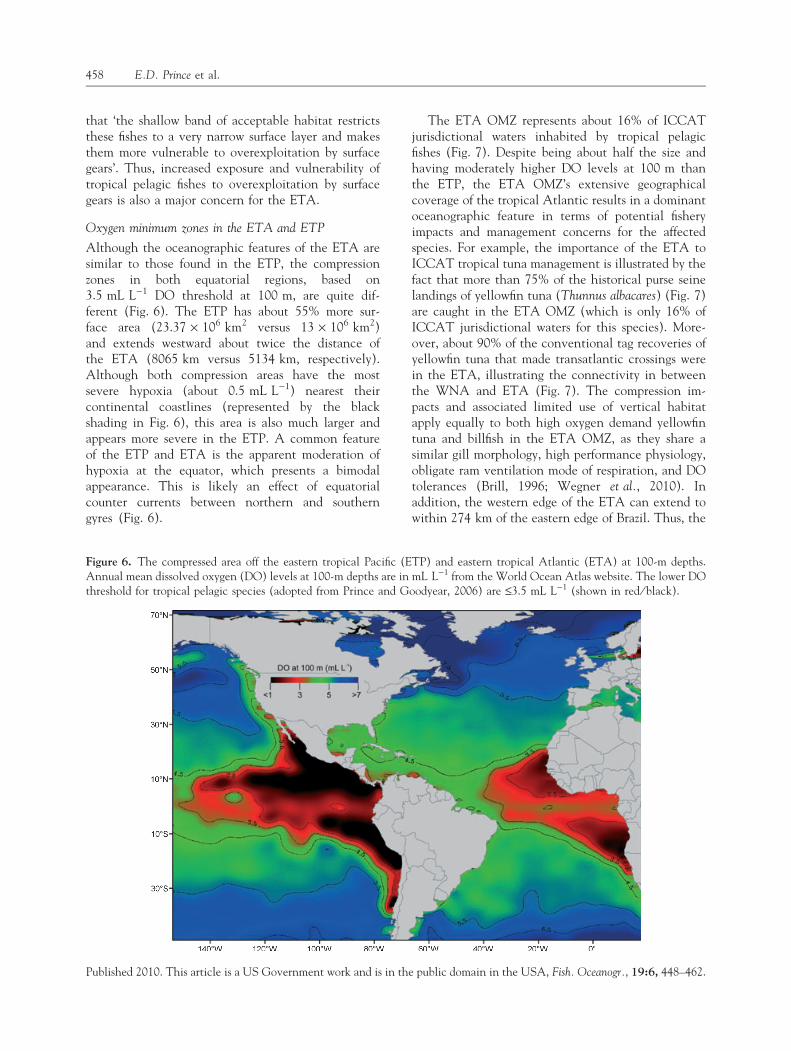
Although the oceanographic features of the ETA aresimilar to those found in the ETP, the compressionzones in both equatorial regions, based on3.5 mL L)1 DO threshold at 100 m, are quite dif-ferent (Fig. 6). The ETP has about 55% more sur-face area (23.37 · 106 km2 versus 13 · 106 km2)and extends westward about twice the distance ofthe ETA (8065 km versus 5134 km, respectively).Although both compression areas have the mostsevere hypoxia (about 0.5 mL L)1) nearest theircontinental coastlines (represented by the blackshading in Fig. 6), this area is also much larger andappears more severe in the ETP. A common featureof the ETP and ETA is the apparent moderation ofhypoxia at the equator, which presents a bimodalappearance. This is likely an effect of equatorialcounter currents between northern and southerngyres (Fig. 6).

The ETA OMZ represents about 16% of ICCATjurisdictional waters inhabited by tropical pelagicfishes (Fig. 7). Despite being about half the size andhaving moderately higher DO levels at 100 m thanthe ETP, the ETA OMZ’s extensive geographicalcoverage of the tropical Atlantic results in a dominantoceanographic feature in terms of potential fisheryimpacts and management concerns for the affectedspecies. For example, the importance of the ETA toICCAT tropical tuna management is illustrated by thefact that more than 75% of the historical purse seinelandings of yellowfin tuna (Thunnus albacares) (Fig. 7)are caught in the ETA OMZ (which is only 16% ofICCAT jurisdictional waters for this species). More-over, about 90% of the conventional tag recoveries ofyellowfin tuna that made transatlantic crossings werein the ETA, illustrating the connectivity in betweenthe WNA and ETA (Fig. 7). The compression im-pacts and associated limited use of vertical habitatapply equally to both high oxygen demand yellowfintuna and billfish in the ETA OMZ, as they share asimilar gill morphology, high performance physiology,obligate ram ventilation mode of respiration, and DOtolerances (Brill, 1996; Wegner et al., 2010). Inaddition, the western edge of the ETA can extend towithin 274 km of the eastern edge of Brazil. Thus, the

Figure 6. The compressed area off the eastern tropical Pacific (ETP) and eastern tropical Atlantic (ETA) at 100-m depths.Annual mean dissolved oxygen (DO) levels at 100-m depths are in mL L)1 from the World Ocean Atlas website. The lower DOthreshold for tropical pelagic species (adopted from Prince and Goodyear, 2006) are £3.5 mL L)1 (shown in red ⁄ black).



ETA 3.5 mL L)1 oxycline at 100 m covers nearly allequatorial Atlantic waters. This is not the case for theETP (Fig. 6), a consequence likely due to the disparity

in size of the two ocean basins (Pacific being muchlarger).

Compression impacts and the stock assessment process

Because habitat compression effectively increases fishconcentrations near the surface, the rate at which fishare caught as a result of one unit of effort will be differentfor the same gear when it is fished inside versus outsidethe compressed area. In other words, compressed habi-tat will have a higher density of tropical pelagic pre-dators and their preferred prey per cubic meter of water.This, in turn, presents implications when using catchper unit effort as an index of relative abundance. Forexample, with longline fishing gear, most of the hooksare distributed shallower than 100 m due to the cate-nary geometry of the longline (Rice et al., 2007). Incompressed habitat, the hook and fish encounter ratewill increase significantly as fish distributions are com-pressed to the 100 m surface layer as compared to thedistribution (0–300 +m) in uncompressed habitat.

Two possible hypothesized relationships betweenCPUE and abundance are illustrated in Fig. 8. Line (a)

Figure 7. We derived the size of the surface area (12.99 · 106 km2) of the compression zone off West Africa based on theannual mean dissolved oxygen levels at 100-m depths from the World Ocean Atlas 1998–2005 composite. This area representsabout 16% of the total Atlantic ICCAT jurisdictional waters for tropical pelagic billfish and tunas (represented as the areabetween red dashed horizontal lines in the North and South Atlantic). Historical purse seine landings of yellowfin tuna(Thunnus albacares) from the International Commission for the Conservation of Atlantic tunas (ICCAT), 1958–2005. Size ofyellow circles is proportional to metric tons. Displacement vectors (white lines ⁄ arrows) indicates transatlantic movementsof yellowfin tuna tagged in the U.S. western North Atlantic with conventional tags and recovered inside the compressed area offWest Africa (tropical eastern Atlantic).

Figure 8. The hypothesized relationship between catch perunit effort (CPUE) and abundance for tropical pelagic bill-fish and tuna in uncompressed (a) and compressed (b)environments (e.g., hypoxia-based habitat compression viaoxygen minimum zones).



depicts the relationship in an uncompressed habitat,and line (b) the relationship in an area of habitatcompression. Both illustrate the assumed proportionalrelationship between CPUE and relative abundance(Fig. 8). These trends are consistent with purse seineexperiments showing elevated catch rates and in-creased vulnerability of tropical tunas inside ETP andETA OMZs, compared to outside these areas (Murphyand Niska, 1953; Brock, 1959; Green, 1967; Sharp,1978; Evans et al., 1981; Sund et al., 1981). In otherwords, at an equivalent level of abundance, the CPUEin the compressed area will be higher than that of theuncompressed habitat simply due to the differences insampled density (Fig. 8). If data from the two habitattypes are inappropriately combined into one estimateof CPUE for the entire area, it will lead to an inac-curate estimate of catchability and, subsequently,inaccurate historic estimations of the index of relativeabundance of the stock. Furthermore, the resultingindex of relative abundance would be even moreinaccurate to the stock assessment result if the OMZswere to expand and shoal closer to the surface overtime (Stramma et al., 2008). However, if the CPUEdata is partitioned by the two different habitat typesand a separate catchability can be reasonably assumedor estimated for each, the inaccuracy can be mini-mized. This suggests that CPUE standardization ofdata from the same fishery ⁄ gear ⁄ target from inside andoutside a compression area should be handled sepa-rately.

If these relationships between CPUE and ocean-ography (Fig. 8) are confirmed, it would be importantto develop separate indices of relative abundance foreach habitat, particularly if the exploitation patternsare different. If the assessment model structure canreplicate the spatial structure of the habitats, thenseparate or spatially interpreted indices can and shouldbe applied to each area ⁄ habitat. There are alreadyseveral assessment models that include specific spatialstructure (catch statistical models such as CASAL,Stock Synthesis, Multifan-CL; and Age structuremodels like VPA2BOX) and others that attemptdirect incorporation of the habitat environmentalconditions (e.g., STATHBS). However, the mainlimitation of these applications is usually the transferof fish between areas within the temporal stratifica-tion, although tagging experiments can provideinformation to infer movement rates.

Alternatively, habitat compression issues can beaddressed directly in the standardization of catchrates. In principle, catch should be stratified spatiallyfor similar vertical habitat structure, with depth ofcapture used as a proxy for different compression

habitats. For example, depth can be inferred in somesituations from the gear configuration (e.g., thenumber of hooks between floats or the theoreticalcatenary shape of longline gear). However, experi-ments with electronic depth recorders on longlinegear have shown that actual depth of the fishing gearis highly variable and dependent on oceanographicconditions, longline interactions with shipping orvery large fish, etc. (Rice et al., 2007). Other proxiesfor different habitats could be inferred from meanDO maps (Fig. 6), depth of thermocline as a functionof time and area, or even temperature at depth pro-files (Prince and Goodyear, 2006). The same strati-fication criteria could then be used for the definitionof the spatial explanatory variable (e.g., area) in theCPUE standardization. The standardization modelshould also evaluate possible changes of the catch-ability factor as a function of time. This can be doneby testing for significant interactions between year ⁄area variables.

The above approach is clearly applicable to pela-gic longline gear fisheries. However, because the sizeof the Atlantic habitat compression covers such alarge area (13 · 106 km2, Fig. 7) this phenomenonalso greatly affects other gears. Not surprisingly, sur-face-oriented gears such as bait-boat and purse seinesoperate almost exclusively in compressed habitatareas (Fig. 7), where the stocks are more available tothese types of gears (Prince and Goodyear, 2006).Developing indices for these gears should berestricted to specific habitat areas, using similar cri-teria for defining these areas, as described above.Attempting ocean-scale standardized indices ofabundance, as described here, is likely to requireadditional research for practical application in theassessment process.

Climate change, global warming, oceanic acidification, andoxygen minimum zones

The impacts of the ETP and ETA OMZs on themanagement of tropical pelagic fishes should not beunderstated. This is particularly relevant consideringthe escalated pace of global warming and concurrentrise in ocean temperatures that would increase thesize, hypoxic severity, and shoaling of these OMZs inthe future (Rosa and Seibel, 2008; Stramma et al.,2008, 2009). The synergistic effects of global warm-ing and ocean acidification, relative to expansion ofthe OMZs, on high oxygen-demand tropical pelagicfishes and their preferred prey will predictably furtherreduce suitable habitat (Rosa and Seibel, 2008;Stramma et al., 2008), while increasing vulnerabilityto higher levels of exploitation by surface fishing



gears (Prince and Goodyear, 2006). It remains to beseen whether the likely expansion of OMZs withglobal warming increases exploitation rates or ratherdilutes the stocks sufficiently so that exploitation islittle affected or declines. Therefore, the populationstatus of tropical pelagic fishes in these areas shouldbe monitored vigilantly to insure these stocks are notfurther diminished. In this regard, incorporatingcompression impacts into the stock assessment pro-cess seems essential, given the extensive geographicalcoverage of these oceanographic features in thetropical Atlantic and the escalated rate of globalwarming that will likely exacerbate future compres-sion impacts.

ACKNOWLEDGEMENTS

We are indebted to the many fishery constituents whoprovided financial and logistical support through ourAdopt-A-Billfish Program. This was essential in pur-chasing PSAT tags as well as in deployment of tagswithin the study areas. Drs. Brian Luckhurst andRussell Nelson assisted in deployment of many of thePSATs. We thank Dr. Andrew Bakun for his expertadvice on oceanography, especially the processes thatled to the development of oxygen minimum zones, aswell as Dr. Michael Prager for his comments on thedraft manuscript. Lastly, we thank Ellen Peel of TheBillfish Foundation (TBF), as well as the TBF board ofdirectors, particularly Mr. Richard Andrews, who soenthusiastically supported the study and field opera-tions. TBF also supported part of C.P. Goodyear’scontribution to the work.

REFERENCES

Anon (2006) US Department of Commerce, National Oceanicand Atmospheric Administration, National GeophysicalData Center. 2-minute Gridded Global Relief Data (ETO-PO2v2).http://www.ngdc.noaa.gov/mgg/fliers/06mgg01.html.H. E.

Antonov, J.I., Locarnini, R.A., Boyer, T.P., Mishonov, A.V. andGarcia, H.E. (2006) World Ocean Atlas 2005, Volume 2:Salinity, edited by S. Levitus, NOAA Atlas NESDIS 62,Washington, D.C.: U.S. Government Printing Office, pp.182.

Bakun, A. (1996) Patterns in the Ocean: Ocean Processes andMarine Populations Dynamics California, USA: University ofCalifornia Sea Grant, San Diego, in cooperation with Cen-tro de Investigaciones Biologicas de Noroeste, La Paz, BajaCalifornia Sur, Mexico, pp. 323.

Bakun, A., Csirke, J., Belda, D.L. and Ruiz, R.S. (1999) ThePacific central American coastal LME. In: Large MarineEcosystems of the Pacific rim, Assessment, Sustainability andManagement. K. Sherman & Q. Tan (eds) Malden, MA:Blackwell Science, pp. 268–280.

Bigelow, K.A. and Maunder, M.N. (2007) Does habitat or depthinfluence the catch rates of pelagic fishes? Can. J. Fish.Aquat. Sci. 64:1581–1594.

Bograd, S.J., Castro, C.D., Lorenzo, E.D. et al. (2008) Oxygendeclines and the shoaling of the hypoxic boundary in theCalifornia current. Geophys. Res. Lett. 35:L12607.doi:10.1029/2008GL03418.

Brill, R.W. (1994) A review of temperature and oxygen toler-ance studies of tunas pertinent to fisheries oceanography,movement models and stock assessments. Fish. Oceanogr.3:204–216.

Brill, R.W. (1996) Selective advantages conferred by the highperformance physiology of tunas, billfish, and dolphin fish.Comp. Biochem. Physiol. 113:3–15.

Brill, R.W. and Lutcavage, M.E. (2001) Understanding envi-ronmental influences on movements and depth distributionsof tunas and billfishes can significantly improve populationassessments. Am. Fish. Soc. Symp. 25:179–198.

Brock, V.E. (1959) The tuna resources in relation to oceano-graphic features. U.S. Fish Wildl. Ser. Circ. 65:1–11.

Bushnell, P.G. and Brill, R.W. (1991) Responses of swimmingskipjack (Katsuwonus pelamis) and yellowfin (Thunnusalbacares) to acute hypoxia, and a model of their cardiorespiratory function. Physiol. Zool. 64:787–811.

Cushing, D. (1969) Upwelling and fish production. FAO Fish.Tech. Paper 84:40 pp.

Diaz, R.J. (2001) Overview of hypoxia around the world.J. Environ. Qual. 30:275–281.

Eby, L.A. and Crowder, L.B. (2002) Hypoxia-based habitatcompression in the Neuse River Estuary: context-dependentshifts in behavioral avoidance thresholds. Can. J. Fish.Aquat. Sci. 59:952–965.

Ekau, W., Auel, H., Portner, H.-O. and Gilbert, D. (2009)Impacts of hypoxia on the structure and processes in thepelagic community (zooplankton, macro-invertebrates andfish). Biogeosci. Discuss. 6:5073–5144.

Evans, R.H., McLain, R.A. and Bauer, R.A. (1981) Atlanticskipjack tuna: influences of mean environmental conditionson their vulnerability to surface fishing gear. Mar. Fish. Rev.43:1–11.

Fonteneau, A. (1997) Atlas of Tropical Tuna Fisheries. WorldCatches and Environment. Paris Cedex, France: ORSTOMeditions, pp.192.

Garcia, H.E., Locarnini, R.A., Boyer, T.P. and Antonov, J.I.(2006) World Ocean Atlas 2005, Volume 3: Dissolved Oxy-gen, Apparent Oxygen Utilization, and Oxygen Saturation,edited by S. Levitus, NOAA Atlas NESDIS 63, Washington,D.C.: U.S. Government Printing Office, pp. 342.

Gooding, R.M., Neill, W.H. and Dizon, A.E. (1981) Respirationrates and low-oxygen tolerance in skipjack tuna, Katsuwonuspelamis. Fish. Bull. 79:31–48.

Goodyear, C.P. (2003) Tests of robustness of habitat standard-ization abundance indices using blue marlin simulated catch-effort data. Mar. Freshw. Res. 79:369–381.

Goodyear, C.P., Lou, J., Prince, E.D. et al. (2008) Verticalhabitat use of Atlantic blue marlin Makaira nigricans: inter-action with pelagic longline gear. Mar. Ecol. Prog. Ser.365:233–245.

Green, R.E. (1967) Relationship of the thermocline to success ofpurse seining for tuna. Trans. Am. Fish. Soc. 96:126–130.

Hanamoto, E. (1987) Effect of oceanographic environment onbigeye tuna distributions. Bull. Jpn. Soc. Fish. Oceanogr.51:203–216.



Helly, J.J. and Levin, L.A. (2004) Global distribution of natu-rally occurring marine hypoxia on continental margins. DeepSea Res. 1 51:1159–1168.

Hinton, M.G. and Maunder, M.N. (2004) Status of stripedmarlin in the Eastern Pacific Ocean in 2002 and outlook in2003–2004. IATTC Stock Assess. Rep. No. 4. 287–310.

Hinton, M.G. and Nakano, H. (1996) Standardizing catch andeffort statistics using physiological, ecological, or behavioralconstraints and environmental data, with an application toblue marlin (Makaira nigricans) catch and effort data from theJapanese longline fisheries in the Pacific. Bull. IATTC21:171–200.

Hoolihan, J.P. and Luo, J. (2007) Determining summer resi-dence status and vertical habitat use of sailfish (Istiophorusplatypterus) in the Arabian Gulf. ICES J. Mar. Sci. 64:1791–1799.

ICCAT (International Commission for the Conservation ofAtlantic Tunas) (2004) Report of the second ICCAT billfishworkshop. Col. Vol. Sci. Pap. ICCAT 41:587.

Idrisi, N., Capo, T.R., Luthy, S. and Serafy, J.E. (2002)Behavior, oxygen consumption and survival of stressedjuvenile sailfish (Istiophorus platypterus) in captivity. Mar.Fresh. Behav. Physical. 36:51–57.

Ingham, M.C., Cook, S.K. and Hausknecht, K.A. (1977) Oxy-cline characteristics and skipjack tuna distribution in thesoutheastern tropical Atlantic. Fish. Bull. 75:857–865.

Locarnini, R.A., Mishonov, A.V., Antonov, J.I., Boyer, T.P. andGarcia, H.E. (2006) World Ocean Atlas 2005, Volume 1:Temperature, edited by S. Levitus, NOAA Atlas NESDIS61, Washington, D.C.: U.S. Government Printing Office,pp. 182.

Maunder, M.N., Hinton, M.G., Bigelow, K.A. and Langley,A.D. (2006) Developing indices of abundance using hab-itat data in a statistical framework. Bull. Mar. Sci. 79:545–559.

Murphy, G.I. and Niska, E.L. (1953) Experimental tuna purseseining in the Central Pacific. Com. Fish. Rev. 15:1–12.

Nielsen, A., Bigelow, K.A., Musyl, M.K. and Sibert, J.R. (2006)Improving light-based geolocation by including sea surfacetemperature. Fish. Oceanogr. 15:314–325.

Post, J.T., Serafy, J.E., Ault, J.S., Capo, T.R. and DeSylva, D.P.(1997) Field and laboratory observations on larval Atlanticsailfish (Istiophorus platypterus) and swordfish (Xiphias gladi-us). Bull. Mar. Sci. 60:1026–1034.

Prince, E.D. and Goodyear, C.P. (2006) Hypoxia-based habitatcompression of tropical pelagic fishes. Fish. Oceanogr.15:451–464.

Prince, E.D., Ortiz, M., Venizelos, A. and Rosenthal, D.S.(2002) In-water conventional tagging techniques developedby the cooperative tagging center for large highly migratoryspecies. Amer. Fish. Soc. Sym. 30:66–79.

Randall, D.J. (1970) Gas exchange in fish. In: Fish Physiology. TheNervous System, Circulation and Respiration. W.S. Hoar & D.J.Randall (eds) Vol. IV. NY: Academic Press, pp. 253–292.

Rice, P.H., Goodyear, C.P., Prince, E.D., Snodgrass, D. andSerafy, J.E. (2007) Use of catenary geometry to estimatehook depth during near-surface pelagic longline fishing:theory versus practice. North Am. J. Fish. Manag. 27:1148–1161.

Roberts, J.L. (1978) Ram gill ventilation in fish. In: The Physi-ological Ecology of Tunas. G.D. Sharp & A.E. Dizon (eds)New York: Academic Press, pp. 83–88.

Rosa, R. and Seibel, B.A. (2008) Synergistic effects of climate-related variables suggest future physiological impairment in atop oceanic predator. Proc. Natl. Acad. Sci. USA105:20776–20780.

Sharp, G.D. (1978) Behavioral and physiological properties oftunas and their effects on vulnerability to fishing gear. In:The Physiological Ecology of Tunas. G.D. Sharp & A.E. Dizon(eds) New York: Academic Press, pp. 397–450.

Stanley, D.R. and Wilson, C.A. (2004) Effect of hypoxia onthe distribution of fishes associated with a petroleum plat-form off coastal Louisiana. North Am. J. Fish. Manag.24:662–671.

Stramma, L., Johnson, G.C., Sprintal, J. and Mohrholtz, V.(2008) Expanding oxygen-minimum zones in the tropicaloceans. Science 320:655–658.

Stramma, L., Visbeck, M., Brandt, P., Tanhua, T. and Wallace,D. (2009) Deoxygenation in the oxygen minimum zone ofthe eastern tropical North Atlantic. Geophys. Res. Lett.36:L20607. doi:10.1029/2009GL039593.

Sund, P.R., Blackburn, M. and Williams, F. (1981) Tunas andtheir environment in the Pacific Ocean: a review. Oceanogr.Mar. Biol. Annu. Rev. 19:443–512.

Wegner, N.C., Sepulveda, C.A., Bull, K.B. and Graham, J.B.(2010) Gill morphometrics in relation to gas transfer andram ventilation in high-energy demand teleosts: scombridsand billfishes. J. Morphol. 271:36–49.



ocean scale hypoxia-based habitat compression of atlantic

Documents