Ocean Heat and Freshwater Content: in situ measurements to climate indicator

Tim BoyerOcean Climate Lab/National Centers for

Environmental InformationApr. 7, 2015

Ocean Climate Lab Team

Subsurface Unit OCSD/CCOGTim BoyerRicardo LocarniniChristopher PaverIgor SmolyarCharles SunMelissa ZwengAlexandra Grodsky (SciTech)Alexey Mishonov (CICS)Jim Reagan (CICS)

Marine Ecosystems Unit OCSD/CCOGOlga BaranovaRost ParsonsDan Seidov

Surface Unit OCSD/CCOGDaphne Johnson

Archive Branch DSDCarla Coleman

Hartmann, D.L., A.M.G. Klein Tank, M. Rusticucci, L.V. Alexander, S. Brönnimann, Y. Charabi, F.J. Dentener, E.J. Dlugokencky, D.R. Easterling, A. Kaplan, B.J. Soden, P.W. Thorne, M. Wild and P.M. Zhai, 2013: Observations: Atmosphere and Surface. In: Climate Change 2013: The Physical Science Basis. Contribution of Working Group I to the Fifth Assessment Report of the Intergovernmental Panel on Climate Change [Stocker, T.F., D. Qin, G.-K. Plattner, M. Tignor, S.K. Allen, J. Boschung, A. Nauels, Y. Xia, V. Bex and P.M. Midgley (eds.)]. Cambridge University Press, Cambridge, United Kingdom and New York, NY, USA, pp. 159–254, doi:10.1017/CBO9781107415324.008

Figure 2.11: | Global mean energy budget under present-day climate conditions. Numbers state magnitudes of the individual energy fluxes in W m–2, adjusted within their uncertainty ranges to close the energy budgets. Numbers in parentheses attached to the energy fluxes cover the range of values in line with observational constraints. (Adapted from Wild et al., 2013.)

Hartmann, D.L., A.M.G. Klein Tank, M. Rusticucci, L.V. Alexander, S. Brönnimann, Y. Charabi, F.J. Dentener, E.J. Dlugokencky, D.R. Easterling, A. Kaplan, B.J. Soden, P.W. Thorne, M. Wild and P.M. Zhai, 2013: Observations: Atmosphere and Surface. In: Climate Change 2013: The Physical Science Basis. Contribution of Working Group I to the Fifth Assessment Report of the Intergovernmental Panel on Climate Change [Stocker, T.F., D. Qin, G.-K. Plattner, M. Tignor, S.K. Allen, J. Boschung, A. Nauels, Y. Xia, V. Bex and P.M. Midgley (eds.)]. Cambridge University Press, Cambridge, United Kingdom and New York, NY, USA, pp. 159–254, doi:10.1017/CBO9781107415324.008

Figure 2.11: | Global mean energy budget under present-day climate conditions. Numbers state magnitudes of the individual energy fluxes in W m–2, adjusted within their uncertainty ranges to close the energy budgets. Numbers in parentheses attached to the energy fluxes cover the range of values in line with observational constraints. (Adapted from Wild et al., 2013.)

5

Changes in Earth’s Heat Balance Components (1022 J) During 1955-2003 (from Levitus, Antonov and Boyer, 2005, GRL)

83% or 0.5 W/m2

How is Ocean Heat Content Changing?

How do we reliably estimate the change?Levitus, S., et al. (2012), World ocean heat content and thermosteric sea level change (0–2000 m), 1955–2010, Geophys. Res. Lett., 39, L10603, doi:10.1029/2012GL05110

The Global Water Cycle

From The Global Water Cycle – Revising the Historical Representation: R. Schmitt http://www.whoi.edu/sbl/liteSite.do?litesiteid=18912&articleId=28329

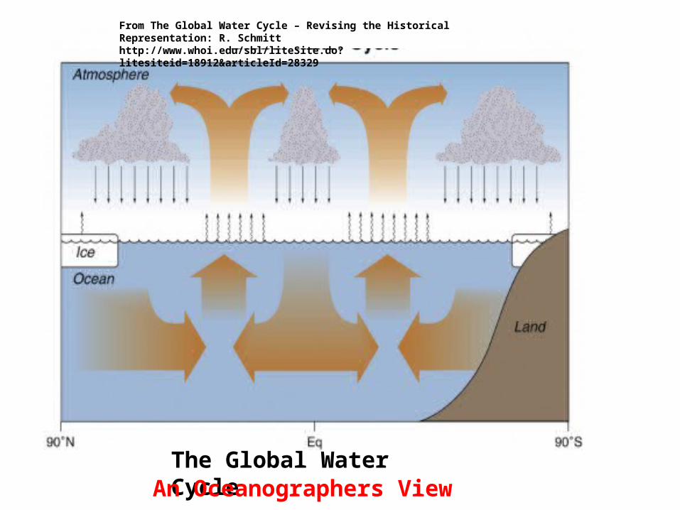
The Global Water CycleAn Oceanographers View

From The Global Water Cycle – Revising the Historical Representation: R. Schmitt http://www.whoi.edu/sbl/liteSite.do?litesiteid=18912&articleId=28329

Water Cycle Intensification: The salty getting saltier, the fresh getting fresher

10

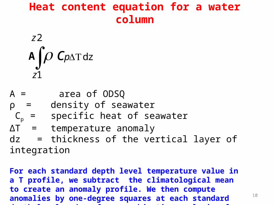
Heat content equation for a water column

dz

2

1

p

z

z

c

A = area of ODSQ ρ = density of seawater Cp = specific heat of seawaterΔT = temperature anomalydz = thickness of the vertical layer of integration

For each standard depth level temperature value in a T profile, we subtract the climatological mean to create an anomaly profile. We then compute anomalies by one-degree squares at each standard depth level and perform an objective analysis of each level.

A

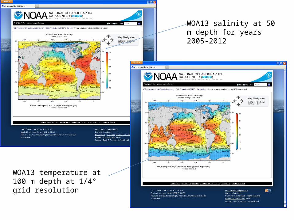
WOA13 salinity at 50 m depth for years 2005-2012

WOA13 temperature at 100 m depth at 1/4° grid resolution

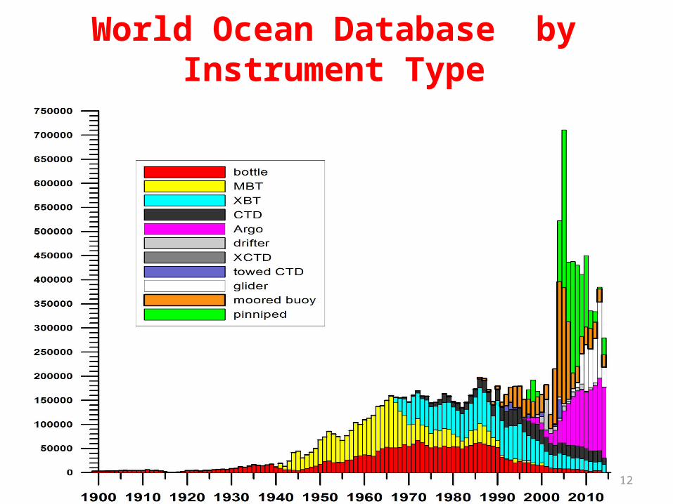
World Ocean Database by Instrument Type

12

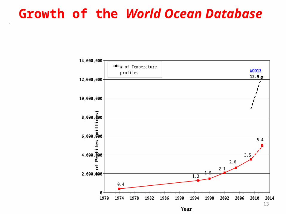
Growth of the World Ocean Database

131970 1974 1978 1982 1986 1990 1994 1998 2002 2006 2010 20140

2,000,000

4,000,000

6,000,000

8,000,000

10,000,000

12,000,000

14,000,000

0.4

1.31.5

2.1

2.6

3.5

# of Temperature profiles

# of Salinity profiles

Year

# of

Pro

files

(mill

ions

)

WOD13 12.9

5.4

(1a) OSD: 2,530,868 profiles (1b) MBT: 2,427,277 profiles (1c) XBT: 2,109,400 profiles (1d) CTD: 634,976 profiles

(1e) UOR: 88,184 profiles (1f) PFL: 520,816 profiles (1g) MRB: 566,540 profiles (1h) DRB: 122,226 profiles

(1i) APB: 89,558 profiles (1j) GLD: 5,857 profiles (1k) SUR: 9,178 profiles (1l) Plankton: 230,944 profiles

World Ocean Database: World’s largest publicly available oceanographic profile database

147,833 Argo cyclesfrom Coriolis DAC

From GTSPP:16,173 XBT14,5219 CTD 3,970 pinniped*20,499 glider

Other sources:CCHDO, ICES, PIRATA, SOOP,North Fisheries, IMOS gliders, Ice buoy,CalCOFI, NIWA (New Zealand) more to come.

Input Data for Ocean Heat/SaltContent Calculations for year2013 (received to date)

*Only used in test version at present

Temperature and salinity anomaly fields (from mean World Ocean Atlas 2009 climatology) calculated using input data for 2013.

Shown are annual anomaly fields for 2013 at 100 m depth. Fields are calculated for 26 discrete depths surface to 2000 m for seasonal, annual, and pentadal (five year) time periods.

Blue=colder/fresher than meanRed=warmer/saltier than mean

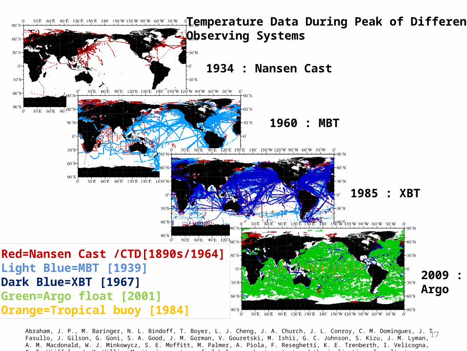
1934 : Nansen Cast

1960 : MBT

1985 : XBT

2009 :Argo

Temperature Data During Peak of DifferentObserving Systems

Red=Nansen Cast /CTD[1890s/1964]Light Blue=MBT [1939]Dark Blue=XBT [1967]Green=Argo float [2001]Orange=Tropical buoy [1984]

17Abraham, J. P., M. Baringer, N. L. Bindoff, T. Boyer, L. J. Cheng, J. A. Church, J. L. Conroy, C. M. Domingues, J. T. Fasullo, J. Gilson, G. Goni, S. A. Good, J. M. Gorman, V. Gouretski, M. Ishii, G. C. Johnson, S. Kizu, J. M. Lyman, A. M. Macdonald, W. J. Minkowycz, S. E. Moffitt, M. Palmer, A. Piola, F. Reseghetti, K. E. Trenberth, I. Velicogna, S. E. Wijffels, J. K. Willis: Monitoring systems of global ocean heat content and the implications for climate change, a review. - Review of Geophysics, Vol. 51, pp 450-483

18

Data from international projects

Left: GEOSECS bottle

and CTD data (1972-1979)

Right: WOCE CTD data

(1990-1998)

19

Data from universities, fisheries

Left: Bottle data from

Hokkaido University (Japan)

(1962-1994)

Right: Temperature Data from

US National Marine Fisheries

(1964-1997)

20

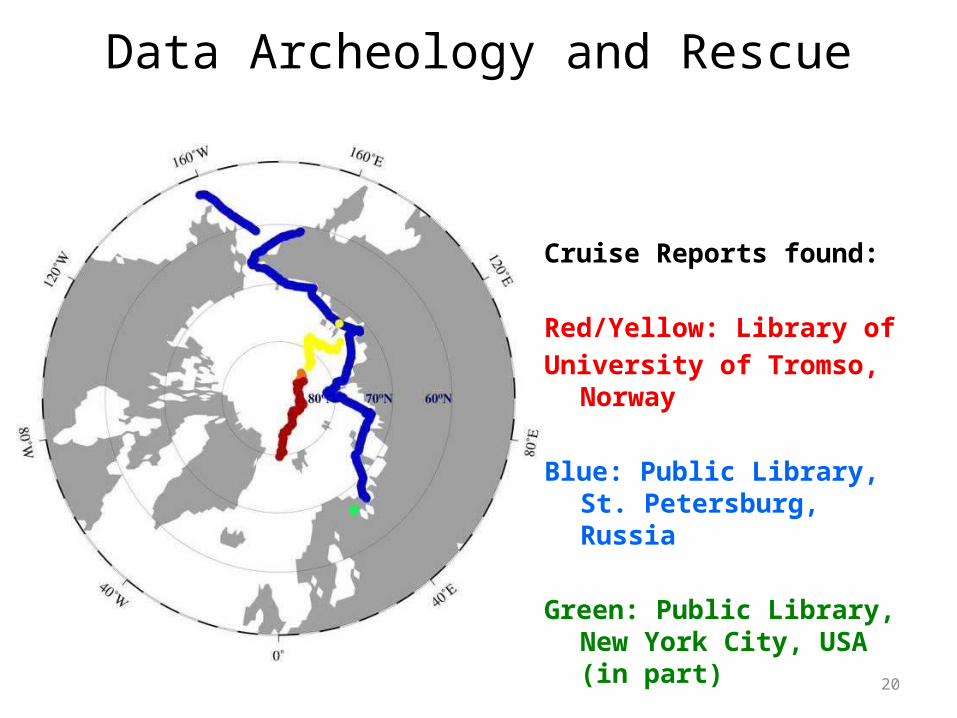
Data Archeology and Rescue

Cruise Reports found:

Red/Yellow: Library of

University of Tromso, Norway

Blue: Public Library, St. Petersburg, Russia

Green: Public Library, New York City, USA (in part)

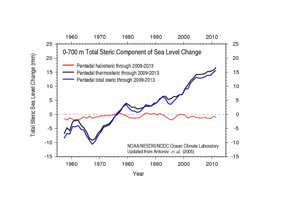
Levitus, S., et al. (2012), World ocean heat content and thermosteric sea level change (0–2000 m), 1955–2010, Geophys. Res. Lett., 39, L10603, doi:10.1029/2012GL05110

Sarah G. Purkey and Gregory C. Johnson, 2010: Warming of Global Abyssal and Deep Southern Ocean Waters between the 1990s and 2000s: Contributions to Global Heat and Sea Level Rise Budgets*. J. Climate, 23, 6336–6351. doi: http://dx.doi.org/10.1175/2010JCLI3682.1

Mean local heat fluxes (a) and thermosteric sea level (b) through 4000 m implied by abyssal warming below 4000 m from the 1990s to the 2000s

24

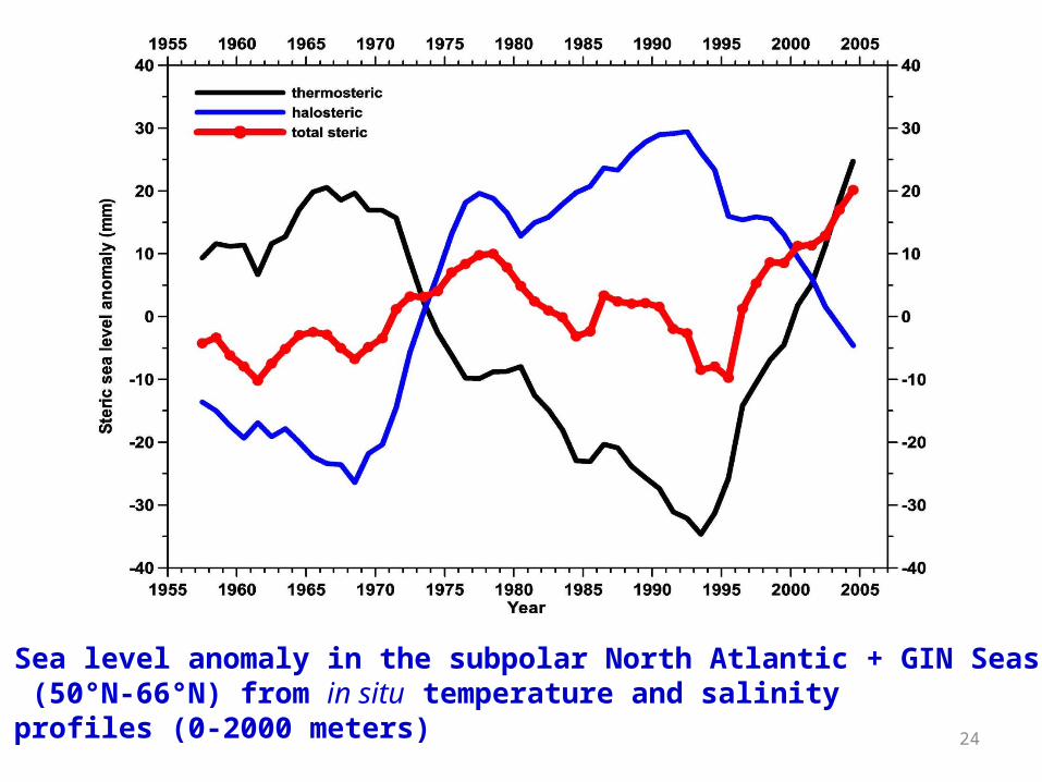
Sea level anomaly in the subpolar North Atlantic + GIN Seas (50°N-66°N) from in situ temperature and salinity profiles (0-2000 meters)

25

Science andData Community

Convert Data to CommonFormat/Initial Quality Control

Calculate ClimatologiesSecondary Quality Control

Release DatabaseWith Quality Control Flags

Scientific ResearchPost-release Quality ControlMonthly database updates

OCL/NCEIMAKE DATA AVAILABLE

Publish Results

FEEDBACK LOOP