ocean haline skin layer and turbulent surface...

Ocean haline skin layer and turbulent surface convections

Y. Zhang1,2 and X. Zhang1

Received 22 July 2011; revised 15 February 2012; accepted 22 February 2012; published 11 April 2012.

[1] The ocean haline skin layer is of great interest to oceanographic applications,while its attribute is still subject to considerable uncertainty due to observationaldifficulties. By introducing Batchelor micro-scale, a turbulent surface convection modelis developed to determine the depths of various ocean skin layers with same modelparameters. These parameters are derived from matching cool skin layer observations.Global distributions of salinity difference across ocean haline layers are then simulated,using surface forcing data mainly from OAFlux project and ISCCP. It is found that, eventhough both thickness of the haline layer and salinity increment across are greater thanthe early global simulations, the microwave remote sensing error caused by the halinemicrolayer effect is still smaller than that from other geophysical error sources. It is shownthat forced convections due to sea surface wind stress are dominant over free convectionsdriven by surface cooling in most regions of oceans. The free convection instability islargely controlled by cool skin effect for the thermal microlayer is much thicker andbecomes unstable much earlier than the haline microlayer. The similarity of the globaldistributions of temperature difference and salinity difference across cool and haline skinlayers is investigated by comparing their forcing fields of heat fluxes. The turbulentconvection model is also found applicable to formulating gas transfer velocity at low wind.

Citation: Zhang, Y., and X. Zhang (2012), Ocean haline skin layer and turbulent surface convections, J. Geophys. Res., 117,C04017, doi:10.1029/2011JC007464.

1. Introduction

[2] Along with the sea surface temperature (SST), the seasurface salinity (SSS) is a major factor in contributing tochanges in density of sea surface water and therefore toocean circulations [Webster, 1994]. Also, a precise temporaland spatial monitoring of SSS provides us a way to trace thefreshwater transport between the ocean and atmosphere dueto evaporation and precipitation, and to gain better knowl-edge of both the climate change and global water cycle. Twosatellite missions with capability of sea surface salinityremote sensing are under way to provide unprecedentedglobal maps of SSS. At the dawn of a new era of remotesensing of SSS, we revisit some aspects of ocean halineskin layer.[3] Much attention has been focused on ocean cool skin

for it has a distinct impact on the absolute accuracy ofremote sensing of SST [Harris et al., 1995]. The tempera-ture difference across cool skin layer, DT, throughout thispaper, is defined as the difference between subsurface andinterface temperatures and is positive when interface tem-perature is lower than subsurface temperature. SinceWoodcock and Stommel [1947] observed and measured the

thermal skin layers, there have been extensive empirical andtheoretical investigations in an effort to improve the absoluteaccuracy of the satellite measurements of SST by taking DTinto account and to better understand surface processesaffecting air-sea gas exchanges.[4] Various models have been proposed over the past fifty

years to account for the complex processes that regulate thethermal sublayer. One group of theories focus on determin-ing the characteristic depth of thermal sublayer dT[Saunders, 1967; Hasse, 1971; Grassl, 1976; Katsaros,1980; Fairall et al., 1996]. DT can be found from the sur-face flux boundary condition by assuming that the ratio ofDT to dT is equivalent to surface temperature gradient,

DT ¼ Q0

rcpkTdT ; ð1Þ

where kT is the molecular diffusivity for temperature. Thetotal skin cooling flux, Q0, is the sum of the latent heat flux,Ql, sensible heat flux, Qs, and long wave radiation, Qlr (Allheat fluxes are defined positive when they direct upwardsthroughout this paper). The density of seawater is r, and thespecific heat capacity is cp. Saunders [1967] proposed thatthe cool skin thickness is inversely proportional to the fric-tion velocity under forced surface convections. Under verylight wind and strong surface cooling, free convectionsbecome dominant and the subject has been subsequentlystudied by Foster [1971], Katsaros et al. [1977], andKatsaros [1980]. Taking into consideration of both free andforced convections, Fairall et al. [1996] proposed that the

1Scripps Institution of Oceanography, University of California,San Diego, La Jolla, California, USA.

2College of Civil Engineering and Architecture, Zhejiang University,Hangzhou, Zhejiang, China.

Copyright 2012 by the American Geophysical Union.0148-0227/12/2011JC007464

JOURNAL OF GEOPHYSICAL RESEARCH, VOL. 117, C04017, doi:10.1029/2011JC007464, 2012

C04017 1 of 15

http://dx.doi.org/10.1029/2011JC007464

cool skin thickness is proportional to the Kolmogorovmicro-scale. Handler et al. [2003] and Wells et al. [2009]investigated the thermal sublayer thickness problem whenthe molecular diffusion is balanced by the surface diver-gence of background large flow structures.[5] The other group of theories [Danckwerts, 1951;

Brutsaert, 1975; Liu et al., 1979; Soloviev and Schlüssel,1994; Castro et al., 2003], often referred as renewal mod-els, determine the cool skin temperature through the renewaltime scale, tr,

DT¼ Q0

rcpkT

ffiffiffiffiffiffiffiffiffitrkT

p: ð2Þ

Soloviev and Schlüssel [1994] proposed a parameterizationfor the renewal time scales in different wind speed regionsregulated by the instabilities of buoyancy, shear, andbreaking waves. Castro et al. [2003] further suggested aparametric model weighting renewal events caused by mul-tiple mechanisms.[6] Without elaborating dynamics of surface processes

that regulates the skin layers, Yu [2010] has examined thepossible importance concerning the SSS remote sensingerror caused by haline skin layers due to surface evaporation.She suggested a magnitude from 0.05 to 0.15 psu formonthly averaged sea surface salinity difference across thesalinity sublayer, DS (in this paper, DS is defined positivewhen top of the haline skin layer is saltier than the bottom).This computation of global DS is based on a modified dif-fusive layer model initially developed by Saunders [1967].The original model has assumed a scaling relationship ofone-third power of diffusivity for skin layer thickness. Fewmodels have been proposed to estimate the sea surface skinsalinity difference, DS, caused by evaporation.[7] Quantifying molecular diffusive layers at ocean sur-

face is also essential to calculating air-sea gas fluxes, asubject highlighted by ocean’s role in taking up a largefraction of fossil fuel-produced carbon dioxide. At sea, gastransfer velocity is controlled by the diffusive layer on thewater side, due to diffusivities of gases of major atmosphericconstitution are much lower in water than in air [Jähne andHaußecker, 1998]. Generalized from cool skin layer para-meterizations, the gas flux, Fc, can be modeled as

Fc ∝kc

dcDC ¼ kcffiffiffiffiffiffiffiffi

kctrp DC; ð3Þ

where DC is aquatic gas concentration difference across thegas diffusive sublayer; kc is the gas molecular diffusivity;and dc is the thickness of the gas diffusive sublayer. Like-wise, ocean salinity sublayer can also be formulated in termsof either the layer depth, dS, or renewal time,

DS ¼ dSE

kS¼ ffiffiffiffiffiffiffiffi

kStrp E

kS; ð4Þ

where kS is the molecular diffusivity of salinity; and E isequivalent surface salinity flux due to evaporation. Thesurface salinity flux equals the rate of evaporation multi-plying surface salinity,

E ¼ QlS0rL

; ð5Þ

where L is the latent heat of evaporation and S0 is the surfacesalinity.[8] In this paper, sea surface cool skin layer and haline

skin layer are both calculated based on a new model whichsupports a layer depth scaling relation of square root ofmolecular diffusivity. The model, constructed to prescribesurface dynamical processes that regulate skin layers, isdescribed in section 2. All input data and model parametersused in our simulations are detailed in section 3. Monthlyaveraged global distributions of nighttime DT, DS andthickness of the skin layers are shown in section 4.Implications of our skin layer calculations are discussed insection 5.

2. A Unified Model for Depth of OceanSkin Layers

[9] Within the ocean surface viscous layer, there are sub-layers of temperature (cool skin layer), salinity (haline skinlayer), and gas concentrations, since the correspondingPrandtl and Schmidt numbers are larger than 1 (Pr = (v/kT) > 1,Sc = (v/kS), (v/kC) > 1, where n is viscosity of seawater).Exactly how sublayer depths related to the molecular diffu-sivity is still an open question.[10] Under persistent surface cooling, the depth of an

established cool skin layer increases initially with time at arate proportional to

ffiffiffiffiffiffiffikT t

pwhen the ocean surface layer is not

disturbed and molecular diffusion dominants. Turbulenteddies can strain, erode or totally destroy the skin layers.Straining may dynamically stabilize the depth of a diffusivelayer as shown by the calculations of Handler et al. [2001]and Wells et al. [2009]. The stabilized layer depth is pro-portional to

ffiffiffiffiffiffiffiffiffickT

p, where c is the local strain rate. Estab-

lished skin layers are eventually broken up or renewed bysurface overturns, caused by instabilities of surface layer dueto buoyancy or shear or by breaking waves and large scalebackground eddies.[11] The surface renewal processes, in many ways, bear

much resemblance to the stirring process in the fluid body byenergetic eddies of large scales. It is the works of combinedmolecular diffusions at very fine scales and turbulent stirringand mixing by larger scale disturbances that attribute to theevolutions of surface skin layer. Therefore, the mean depthof the layer should be related to the statistical balancesbetween molecular diffusivity and those surface stirringprocesses. From this point of view, it is not unexpected thatmost renewal models and turbulence models derive thesimilar parameterizations for ocean skin layer temperature.[12] An early model for the thicknesses of thermal and

salinity sublayers is proposed by Saunders [1967] in whichonly forced convection is considered with parameters of seasurface friction velocity, u*, and surface heat flux, Q0. Thethickness of cool skin layer, dT, is controlled by the viscousstress at surface tv = ru∗

2,

dT ¼ ln�

tnr

� �12

; ð6Þ

where l is Saunders’ coefficient which is fairly constant asindicated by different observations. Analogy to solid wallboundary layer, Saunders adopted a one third power of dif-fusivity law for determining salinity sublayer thickness.

ZHANG AND ZHANG: OCEAN HALINE SKIN LAYER C04017C04017

2 of 15

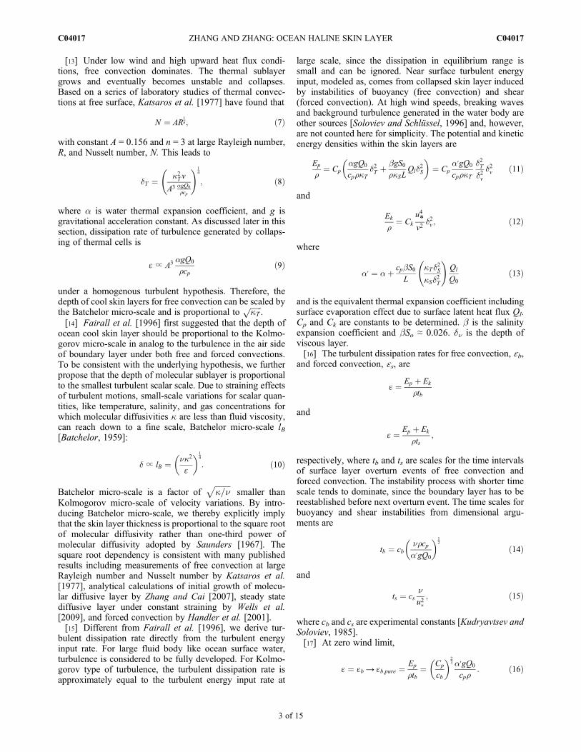
[13] Under low wind and high upward heat flux condi-tions, free convection dominates. The thermal sublayergrows and eventually becomes unstable and collapses.Based on a series of laboratory studies of thermal convec-tions at free surface, Katsaros et al. [1977] have found that

N ¼ AR1n; ð7Þ

with constant A = 0.156 and n = 3 at large Rayleigh number,R, and Nusselt number, N. This leads to

dT ¼ k2T v

A3 agQ0

rcp

!14

; ð8Þ

where a is water thermal expansion coefficient, and g isgravitational acceleration constant. As discussed later in thissection, dissipation rate of turbulence generated by collaps-ing of thermal cells is

ɛ ∝ A3 agQ0

rcpð9Þ

under a homogenous turbulent hypothesis. Therefore, thedepth of cool skin layers for free convection can be scaled bythe Batchelor micro-scale and is proportional to

ffiffiffiffiffiffikT

p.

[14] Fairall et al. [1996] first suggested that the depth ofocean cool skin layer should be proportional to the Kolmo-gorov micro-scale in analog to the turbulence in the air sideof boundary layer under both free and forced convections.To be consistent with the underlying hypothesis, we furtherpropose that the depth of molecular sublayer is proportionalto the smallest turbulent scalar scale. Due to straining effectsof turbulent motions, small-scale variations for scalar quan-tities, like temperature, salinity, and gas concentrations forwhich molecular diffusivities k are less than fluid viscosity,can reach down to a fine scale, Batchelor micro-scale lB[Batchelor, 1959]:

d ∝ lB ¼ nk2

ɛ

� �14

: ð10Þ

Batchelor micro-scale is a factor offfiffiffiffiffiffiffiffik=n

psmaller than

Kolmogorov micro-scale of velocity variations. By intro-ducing Batchelor micro-scale, we thereby explicitly implythat the skin layer thickness is proportional to the square rootof molecular diffusivity rather than one-third power ofmolecular diffusivity adopted by Saunders [1967]. Thesquare root dependency is consistent with many publishedresults including measurements of free convection at largeRayleigh number and Nusselt number by Katsaros et al.[1977], analytical calculations of initial growth of molecu-lar diffusive layer by Zhang and Cai [2007], steady statediffusive layer under constant straining by Wells et al.[2009], and forced convection by Handler et al. [2001].[15] Different from Fairall et al. [1996], we derive tur-

bulent dissipation rate directly from the turbulent energyinput rate. For large fluid body like ocean surface water,turbulence is considered to be fully developed. For Kolmo-gorov type of turbulence, the turbulent dissipation rate isapproximately equal to the turbulent energy input rate at

large scale, since the dissipation in equilibrium range issmall and can be ignored. Near surface turbulent energyinput, modeled as, comes from collapsed skin layer inducedby instabilities of buoyancy (free convection) and shear(forced convection). At high wind speeds, breaking wavesand background turbulence generated in the water body areother sources [Soloviev and Schlüssel, 1996] and, however,are not counted here for simplicity. The potential and kineticenergy densities within the skin layers are

Ep

r¼ Cp

agQ0

cprkTd2T þ bgS0

rkSLQld2S

� �¼ Cp

a′gQ0

cprkT

d2Td2v

d2v ð11Þ

and

Ek

r¼ Ck

u4*v2

d2v ; ð12Þ

where

a′ ¼ aþ cpbS0L

kTd2SkSd2T

!Ql

Q0ð13Þ

and is the equivalent thermal expansion coefficient includingsurface evaporation effect due to surface latent heat flux Ql.Cp and Ck are constants to be determined. b is the salinityexpansion coefficient and bSo ≈ 0.026. dn is the depth ofviscous layer.[16] The turbulent dissipation rates for free convection, ɛb,

and forced convection, ɛs, are

ɛ ¼ Ep þ Ek

rtb

and

ɛ ¼ Ep þ Ek

rts;

respectively, where tb and ts are scales for the time intervalsof surface layer overturn events of free convection andforced convection. The instability process with shorter timescale tends to dominate, since the boundary layer has to bereestablished before next overturn event. The time scales forbuoyancy and shear instabilities from dimensional argu-ments are

tb ¼ cbnrcpa′gQ0

� �12

ð14Þ

and

ts ¼ csnu2�

; ð15Þ

where cb and cs are experimental constants [Kudryavtsev andSoloviev, 1985].[17] At zero wind limit,

ɛ ¼ ɛb → ɛb;pure ¼ Ep

rtb¼ Cp

cb

� �23 a′gQ0

cpr: ð16Þ


3 of 15

By comparison, the ratio of constants Cp and cb can berelated to the free convection experimental constant A[Katsaros et al., 1977]:

C1 ¼ Cp

cb

� �23

¼ An: ð17Þ

[18] At high wind and zero surface heat flux limit,

ɛ ¼ ɛs → ɛs;pure ¼ Ek

rts¼ Ck

cs

� �23 u4*n: ð18Þ

Substituting Batchelor micro-scale formula for temperatureinto equation (6), we found that the ratio of constants Ck andcs can be related to the Saunders’ coefficient at the limit ofpure forced convections:

C2 ¼ Ck

cs

� �23

¼ kT

n

� �2 1

l

� �4

: ð19Þ

[19] Introducing a Richardson number defined as the ratioof the turbulent dissipation rate of free convection to that offorced convection,

Ri ¼ ɛbɛs

¼ cscb

� �23 a′gQ0n

cpru4*

!13

¼ C3a′gQ0ncpru4*

!13

: ð20Þ

When Ri > 1, free convection dominates. Otherwise, shear-forced convection becomes important. The value of cb/cs isestimated to vary from 0.012 to 0.028 [Kudryavtsev andSoloviev, 1985; Fairall et al., 1996]. Rewriting dissipationrate in Richardson number, we have

ɛ ¼

ɛb ¼ Ri 1þ C2C33

C1

� �32Ri�3

0B@

1CA

23

C1a′gQ0

rcp

� �Ri > 1

ɛs ¼ 1þ C1

C2C33

� �32Ri3

0B@

1CA

23

C2

u4*n

!Ri < 1

:

8>>>>>>>><>>>>>>>>:

ð21ÞOur expression of dissipation rate includes the proportionalconstant between skin layer thickness and Batchelor micro-scale when we determine the coefficients C1 and C2 bymatching thermal layer thickness. Thus, the proportionalconstant for thickness of sublayer in Batchelor micro-scaleformula (equation (10)) can be set as 1 when the turbulentdissipation rate is given by equation (21).[20] Incorporating free convection to Saunders’ thermal

sublayer parameterization (equation (6)), our modifiedSaunders’ coefficient is

lT ¼lRi�

14C

�14

2 1þ C1

C2C33

� �32Ri3

0B@

1CA

�16

Ri > 1

lC�14

2 1þ C1

C2C33

� �32Ri3

0B@

1CA

�16

Ri < 1

:

8>>>>>>>>><>>>>>>>>>:

ð22Þ

Thus, for the thermal sublayer, DT can be calculated byequation (1) and equation (6) with the modified Saunders’coefficient. For salinity sublayer, we have

DS

S0¼ Ql

rLkS

vk2S

ɛ

� �14

¼ lTkT

kS

� �12 Qlv

u*rLkT: ð23Þ

3. Data and Computation Methods

3.1. Surface Forcing and Environmental Data

[21] Input data for our computations include surface windspeeds at a reference height of 10 m, u10 m; sea surfacetemperature, SST; near sea surface air humidity, SH; meansea surface salinity, S0; and sea surface heat flux compo-nents, including latent heat flux, sensible heat flux, longwave radiation and short wave radiation, Qsr. Qlr and Qsr areacquired from the International Satellite Cloud ClimatologyProject (ISCCP) [Zhang et al., 2004]. A climatologicallymonthly mean sea surface salinity S0 is taken from theWorld Ocean Atlas 2005 [Antonov et al., 2006], and no dailydata is available for SSS. All other daily averaged values ofabove surface forcing data are obtained from the ObjectivelyAnalyzed Air-Sea Fluxes (OAFlux) project at the WoodsHole Oceanographic Institution [Yu and Weller, 2007]. Thedaily data have a spatial resolution of 1� � 1� and cover overthe period from 1988 to 2007. These input data are producedby synthesizing surface meteorology obtained from satelliteremote sensing and atmospheric model reanalyzes outputs.In this work, u* is calculated by COARE 3.0 algorithm. It isassumed that the surface tangential viscous stress is pro-portional to the total wind stress and the proportional con-stant is included in the Saunders’ constant, like in the mostof such practices.

3.2. Coefficients of Seawater and Air Properties

[22] Over the oceans, SST varies from �2�C to 35�C, andSSS ranges from 31 psu to 38 psu mostly. Most of thecoefficients of seawaters and air properties are not verysensitive to the variation of temperature or salinity as far ascalculation accuracy is concerned. Most of the coefficientswith a maximum variation under 10% are treated as con-stants. These include thermal diffusivity of seawater, kT =1.40 � 10�7 m2 s�1; salinity diffusivity, kS = 7.4 � 10�8 m2

s�1; specific heat of seawater, cp = 4.19 � 103 J kg�1 K�1;density of seawater, r = 1.025 � 103 kg m�3; acceleration ofgravity, g = 9.8 m s�2; and latent heat of vaporization, L =2.454 � 106 J kg�1.[23] Two coefficients change more than 10% with the

environment variables, namely thermal expansion coeffi-cient and seawater viscosity. We calculate the equivalentexpansion coefficient of the sea surface water (defined inequation (13)) considering both temperature and salinityvariations (equation (13)). The thermal expansion coefficienthas a strong dependency on SST, and is fitted with a fourthorder polynomial: a = 10�4 � (0.0000181 � SST 3 �0.00175� SST 2 + 0.130� SST + 0.525)�C�1 to the table bySverdrup et al. [1942].[24] Equation (1) and equation (23) show that both DT

and DS are proportional to seawater viscosity, which also


4 of 15

varies with SST. We adopt a third order polynomial fitting:n = (1.773 � 4.565 � 10�6 SST3 + 7.14 � 10�4 SST2 �4.904 � 10�2 SST) � 10�6 m2 s�1, according to the tablefrom www.engineersedge.com/fluid_flow/fluid_data.htm.

3.3. Model Parameters

[25] There are three parameters in our model for depth ofocean skin layer: C1 for buoyancy flux from free convec-tions, C2 for kinetic energy flux from forced convections,and C3 for determining the transition from free to forcedconvection dominance. Their values are estimated based onexisting observations. As shown in section 2, C2 is found tobe related to the Saunders’ constant l at the limit of pureforced convection condition. It has been suggested frommany field observations that l is more or less constant[Paulson and Parker, 1972; Paulson and Simpson, 1981;Coppin et al., 1991]. Grassl [1976] and Schlüssel et al.[1990] presented data indicating that l is weakly windspeeds dependent. We chose l = 6, which falls in the middlerange of field observations, thus C2 = 1.25 � 10�5.[26] C1 is proportional to An at the limit of low wind

speeds when skin layer buoyancy instability dominates.Field observations of A and n are still difficult to obtain.There are extensive observations on thermal convections inlaboratory experiments [Herring, 1963; Foster, 1971;Katsaros et al., 1977; Leighton et al., 2003; Wells et al.,2009]. We take the results from large Rayleigh numbercases with an exponent n = 3 and yield the parameter Avarying from 0.156 to 0.29 [Katsaros et al., 1977; Wellset al., 2009; Leighton et al., 2003]. The particular choiceof its value affects the prediction of skin layer at low winds,which will be discussed later. Here we chose the arithmeticmean of the upper and lower bounds, 0.29 and 0.156: A =0.22, or C1 = 0.0106.[27] C3 is determined by the threshold of transition from

the thermal instability to the shear instability which is con-trolled by the surface forcing fields of Q0 and u*. Fairallet al. [1996] suggested a ratio Q0/u*

4 to be a value of1.59 � 1012 kg m�2 s when the two processes are equallyimportant. Based on laboratory observations of renewal timescales for free and forced convections, Kudryavtsev andSoloviev [1985] found the transition ratio Q0/u*

4 = 3.07 �1011 kg m�2 s. The mean square root of the two ratios ischosen in this paper (Q0/u*

4 = 6.34 � 1011 kg m�2 s), whichleads to our current value of C3 = 14.4.

3.4. Model Comparisons

[28] Under Tropical Ocean–Global Atmosphere CoupledOcean-Atmosphere Response Experiment (TOGA-COARE)field program, Fairall et al. [1996] developed an air-sea fluxalgorithm, which accounts for the light wind and strongconvection conditions over tropical oceans. Their model fortemperature difference DT can be expressed in the sameform as equation (6) and equation (1) with a modifiedSaunders’ coefficient:

lT¼6 1 þ Q024ga′v3

u4*rcpk2T

!" #: ð24Þ

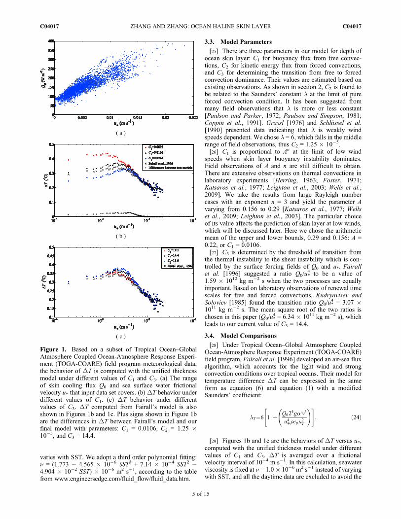
[29] Figures 1b and 1c are the behaviors of DT versus u*,computed with the unified thickness model under differentvalues of C1 and C3. DT is averaged over a frictionalvelocity interval of 10�4 m s�1. In this calculation, seawaterviscosity is fixed at n = 1.0� 10�6 m2 s�1 instead of varyingwith SST, and all the daytime data are excluded to avoid the

Figure 1. Based on a subset of Tropical Ocean–GlobalAtmosphere Coupled Ocean-Atmosphere Response Experi-ment (TOGA-COARE) field program meteorological data,the behavior of DT is computed with the unified thicknessmodel under different values of C1 and C3. (a) The rangeof skin cooling flux Q0 and sea surface water frictionalvelocity u* that input data set covers. (b) DT behavior underdifferent values of C1. (c) DT behavior under differentvalues of C3. DT computed from Fairall’s model is alsoshown in Figures 1b and 1c. Plus signs shown in Figure 1bare the differences in DT between Fairall’s model and ourfinal model with parameters: C1 = 0.0106, C2 = 1.25 �10�5, and C3 = 14.4.


5 of 15

warm layer effect. As for comparison, we also plotted themodel results of Fairall et al. [1996] in Figures 1b and 1c.The meteorological data set used for the plots (Figure 1a) is a

subset of TOGA-COARE field program (provided by C. W.Fairall, private communication, 2011).[30] In Figure 1b, three different values of C1 are used:

0.0038, 0.0106, and 0.0244. They correspond to values of A

Figure 2. Monthly averaged global nighttime distributions of (a) total surface cooling flux Q0, (b) seasurface water friction velocity, u*, and (c) common logarithm of Richardson number, log10Ri, for themonths of February and August. All monthly averaged fields in this paper are averaged over daily fieldsfrom 1998 to 2007. Brown refers to continents, whiles gray refers to areas with no input data.


6 of 15

being 0.156, 0.22, and 0.29 respectively. As shown, asmaller value of A would predict a larger DT at low windspeeds. The output of Fairall’s model falls in between of ourpredictions with A = 0.22 and 0.29. The scattering of DT atlow wind limit is related to the scattering of Q0. At highwind speed limit, all model predictions approach the samevalue by Saunders [1967] as expected.[31] The impact of instability range threshold, C3, on DT

calculations is illustrated in Figure 1c. C3 = 19.1 correspondsto the threshold given by Kudryavtsev and Soloviev [1985],and C3 = 11 corresponds to the threshold given by Fairallet al. [1996]. C3 affects cool skin temperature in a narrowrange where Richardson number is close to 1.[32] Fairall et al. [1996] has reported that his model

underestimates the measured DT, obtained from the tropics,by 0.05�C. At small to moderate wind speeds, a commonwind situation at tropics, our model predict a higher DT byamount of 0.01–0.03�C (Figure 2b).

4. Global Distributions of the Simulation Results

[33] Surface warm layer due to solar radiation, wavebreakings and surfactant effects is not considered in the sim-ulation results shown here. About 20% of solar radiationenergy is absorbed within the top 1 cm seawater. The surfaceheat flux budgets in the daytime and nighttime can be verydifferent. Surface heat flux used below only includes latentheat flux, sensible heat flux and long wave radiation, andtherefore the results can only be applied to nighttime skinlayer. Large-scale wave breakings at high winds are highlyintermittent and the breakers are highly dissipative. Over 90%of the intense turbulent is dissipated within 4 passing wavecrests as suggested by Rapp and Melville [1990]. A plausibleestimate of area affected by breaking waves is the whitecapcoverage. Therefore the area affected by energetic breakingwaves is less than 1% in a wide range of wind speeds.Assuming DT is zero in those area affected by breakingwaves, large-scale wave breaking reduces the area averagedDT by less than 1%. Compared with large-scale wave break-ings, micro-scale wave breakings take place much more fre-quently beginning at moderate wind speeds. Incipientbreaking waves induced by surface drifts disrupt the surfacesublayers and occur sporadically. Flow separations occur nearthe crests of steep short gravity wavelets, and, as a result,vortices are accumulated in the wave crest regions. The cap-illary bores from the micro-scale breaking reduce the DT anddiffusive layer thickness there. Considering a two-dimensionalwavefield, the steep wavelet crests cover roughly 1/10 ofsurface area at most at sea, for the mean slopes of short wavesare only of moderate for large fetches. By the same argumentabove, we assume that micro-scale wave breaking affects DTin less than 10% surface area, therefore, a high order effect onthe area averagedDT.Quantified field observations on micro-scale wave breakings are still not available. Beside wavebreakings, how surfactants affect the surface processes thatregulate surface microlayers is not well understood. In mostopen oceans, the influences by surfactants from surface activematerials are assumed to be statistically small here as indicatedfrom worldwide observations of dissolved organic matters[Hansell et al., 2009].

4.1. Global Nighttime Distributionsof Richardson Number

[34] The surface forcing data from ISCCP and OAFluxproject show following features: Q0 (Figure 2a) is mostlylow at the latitudes higher than 40� except for the regions ofwestern boundary currents and their extensions, and is gen-erally high at latitudes lower than 40�. Q0 varies with sea-sons, and is high in hemisphere winters and is low inhemisphere summers at the corresponding latitudes. Thehighest Q0 happens in winters over western boundary cur-rents that transport warm water from low latitudes to highlatitudes. Wind stress (Figure 2b) is high under Westerliesand the trade winds as expected. There are seasonal cycles ofWesterlies and trade winds in the both Hemispheres, whilethe wind stress is more persistent over the Antarctic Cir-cumpolar current. Low wind speed belts can be found at thehouse latitudes especially in winters. The wind stress overIndia Ocean follows the Monsoon wind cycles. It is thusclear that the input data have strong seasonal variations.Therefore, in this section, we choose February and August asrepresentatives to show the 20 yr-monthly averaged resultsin winter and summer periods.[35] Figure 2c shows monthly averaged global distribu-

tions of the nighttime Richardson number. Since the

Richardson number is proportional to Q0

13 and inversely

proportional to u*43 , wind speed strongly influences the

Richardson number from moderate to high winds. Asexpected, Richardson number is generally low under theWesterly belts and the trade-wind belts due to high winds.Westerlies in Southern Hemisphere are persistent to keepRichardson number small (≪1) there all year-round, whilethe Richardson number in areas under Westerlies in North-ern Hemisphere is small in the winter and moderate to largein the summer. The Richardson number under the tradewinds is also low, especially in the hemisphere winters.Even though the surface heat flux from sea to air is strongunder trades in hemisphere winters, the intensive winds keepthe Richardson number small. There are thin bands ofmoderated Richardson numbers at horse latitudes. The bandsshift polar-ward in summers and equator-ward in winters.Over parts of tropical warm pools, the Richardson number islarge (>1) from October to next March when the SouthAsian Monsoon is inactive. The largest Richardson numberover narrow coastal areas in the north hemisphere summer isdue to both the very low winds and very small heat fluxes ofthe input data set we used. Richardson number over most seaareas, in short, is small to moderate and less than one.[36] Besides wind speed and skin cooling flux, we also

investigated the possible impact of the expansion coefficientand viscosity on Richardson number. These two factors bothvary with SST. At the temperature over 20�C, they canceleach other. They increase the Richardson number at thelatitudes higher than 45� where the SST is low.

4.2. Global Nighttime Distributions of the SalinitySublayer Thickness and Gas Transfer Velocity

[37] As discussed in section 2, one consequence of intro-ducing unified thickness model is that the thickness ratio ofdifferent diffusive sublayers becomes square root of the ratioof the sublayers’ molecular diffusivities. The value of this


7 of 15

ratio is fairly even globally. Thus, only global nighttimedistributions of the salinity sublayer thickness are shown inthe paper. The thickness of the salinity sublayer can beexpanded as:

There is a common factor in both free convection and forcedconvection dominant regions:

u4*vþ C1

C2C33

� �32

C33 a′gQ0

rcp

!:

When Ri < 1,

u4*v

> C33

a′gQ0

rcp:

The first term in the parenthesis is much larger than thesecond term, since

C1

C2C33

� �32

is about 0.15. When forced convection dominates, the skinlayer depth depends mostly on wind stress. As Richardsonnumber increases over 1 (into the free convection dominantregion), surface heat flux becomes increasingly moreimportant while the influence of wind stress diminishesquickly.

[38] Two representative global nighttime distributions ofsalinity sublayer thickness dS are shown in Figure 3. The dShas a globally averaged magnitude around 0.065 mm foreach month. In section 4.1, we find that the sea surface tur-

bulence, over most of the ocean surfaces, is controlled bywind speeds. Thus, in accordance with equation (25), thedistribution of the sublayer thickness should be largelycomplementary to that of wind speeds.[39] In winters, i.e., Northern Hemisphere in February and

Southern Hemisphere in August for instance (Figure 3), theWesterliers and trade winds are extremely strong, the salin-ity sublayer thicknesses over these areas are thinner than0.05 mm. The thin layer regions can expand to cover lati-tudes from 10� to 60� except for the horse latitudes. Oneinteresting feature over these regions is that, although theWesterlies are stronger than the trade winds, the thicknessesof salinity sublayers under them are indeed comparable. Thisis because the sea surface water viscosity under the West-erlies belts is higher than that under the trade-wind belts, dueto decreasing SST with increasing latitudes.[40] In the hemisphere summers, the thin layer regions still

exist, however the total area shrinks. The sea areas at horselatitudes have a band of relatively thick dS. The thickness ofsalinity sublayers in the coastal areas of high latitudes islarge with values around 0.1–0.2 mm due to the very-lowwind from the input data. From December to next May, thereis a band of large thickness, extending from the west coastal

dS ¼v14k

12S C3C2ð Þ�1

4u4*vþ C1

C2C33

� �32

C33 a′gQ0

rcp

!�16 a′gQ0

rcp

� �� 112

;Ri > 1

v14k

12SC2

�14

u4*vþ C1

C2C33

� �32

C33 a′gQ0

rcp

!�16 u4*

v

!� 112

≈ v14k

12SC2

�14

u4*v

!�14

;Ri < 1 :

8>>>>>><>>>>>>:

ð25Þ

Figure 3. Monthly averaged global nighttime distributions of the salinity sublayer thickness dS for themonths of February and August.


8 of 15

areas in the tropics. The thickness can reach as thick as0.15 mm.[41] At sea, gas exchanges between the ocean and atmo-

sphere take place both at sea surface and through bubblesgenerated by breaking waves. The corresponding gas trans-fer velocities for surface and bubble are noted as ks and kb.Direct transfer across the sea surface by a combination ofmolecular and turbulent diffusion depends on the moleculardiffusivity of the dissolved gas. It is widely adopted that inrough water conditions the transfer velocity of a gas will beinversely proportional to the square root of the Schmidtnumber. An empirical form is given by Jähne et al. [1987],based on observations in laboratory wind-wave tanks:

ks ¼ 1:57� 10�4u*600

Sc

� �12

: ð26Þ

[42] Although many commonly used parameterizations forgas transfer velocity are wind speed only formulations, itwas understood that a simple relationship to wind speed orfriction velocity cannot fully account for the variability dueto surface heating and developing wave state, etc. If thesurface transfer velocity is modeled to be proportional to theinverse of skin layer depth as equation (3), we derive aparameterization for ks with the same Schmidt numberdependency for the rough water under low wind speed:

ks ¼u*Sc

12

BRi

14 C2 þ C1C�2

3 Ri3� 1

6 Ri > 1

C2 þ C1C�23 Ri3

� 16u* Ri < 1

:

(ð27Þ

In wind-wave tank experiments, Richardson numbers arenormally below 1 due to small heat fluxes as compared tothe wind stresses. Our model constant B of surface transfervelocity can be found by fitting equation (27)

B ¼ 1:57� 10�4

C2 þ C1C�23 Ri3t

� 16

600ð Þ12; ð28Þ

where Rit is the typical Richardson number in tank experi-ments. At large Richardson numbers, the surface heat fluxbecomes an influential factor.

4.3. Global Nighttime Distributions of Temperatureand Salinity Differences Across the Skin Layers

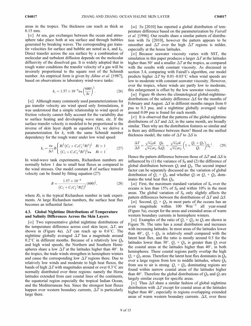
[43] Two representative global nighttime distributions ofthe temperature difference across cool skin layer, DT, areshown in (Figure 4a). DT can reach up to 0.6�C. Thenighttime globally averaged DT has a magnitude around0.2�C in different months. Because of a relatively low Q0

and high wind speeds, the Northern and Southern Hemi-spheres share a low DT at the latitudes higher than 40�. Inthe tropics, the trade winds strengthen in hemisphere wintersand cause the corresponding low DT regions there. Due torelatively low winds and moderate to high heat fluxes, thebands of high DT with magnitudes around or over 0.3�C arenormally distributed over three regions: namely the Horselatitudes extended from east coastal lines of the continents,the equatorial region especially the tropical Indian Ocean,and the Mediterranean Sea. Since the strongest heat fluxeshappen over western boundary currents, DT is particularlylarge there.

[44] Yu [2010] has reported a global distribution of tem-perature difference based on the parameterization by Fairallet al. [1996]. Our results share a similar pattern of distribu-tion with Yu [2010], however the pattern appears to besmoother and DT over the high DT regions is milder,especially at the house latitudes.[45] Because seawater viscosity varies with SST, the

simulation in this paper produces a larger DT at the latitudeshigher than 50� and a smallerDT at the tropics, as comparedwith the results with constant viscosity. As discussed insection 3.4, comparing with Fairall’s algorithm, our modelpredicts higher DT by 0.01–0.03�C when wind speeds arelow to moderate with constant seawater viscosity. However,over the tropics, where winds are partly low to moderate,this enlargement is offset by the low seawater viscosity.[46] Figure 4b shows the climatological global-nighttime-

distributions of the salinity difference DS for the months ofFebruary and August. DS in different months ranges from 0psu to 0.3 psu, and a nighttime globally averaged valuearound 0.09 psu is found for each month.[47] It is observed that the patterns of the global nighttime

distributions of DT and DS, in the same month, are broadlysimilar. Then why are the distribution features so similar andis there any difference between them? Based on the unifiedthickness model, the ratio of DT to DS is

DT

DS¼

ffiffiffiffiffikS

prLffiffiffiffiffiffi

kTp

rcpQ0

S0Ql¼

ffiffiffiffiffikS

prLffiffiffiffiffiffi

kTp

rcp1þ Qs þ Qlr

Ql

� �S�10 : ð29Þ

Hence the pattern difference between those of DT and DS isinfluenced by (1) the variance of S0 and (2) the difference ofglobal distribution between Ql and Q0. The second impactfactor can be separately discussed as: the variation of globaldistribution of Qs + Qlr and whether Ql or Qs + Qlr dom-inates the total heat flux Q0.[48] First, the maximum standard variation of S0 over the

oceans is less than 15% of S0 and within 10% in the mostareas. The global variation of S0 only slightly affects thepattern differences between the distributions of DT and DS.[49] Second, Qs + Qlr in most parts of the oceans has an

even magnitude within 100 Wm�2 all year-round(Figure 5a), except for the areas and extended areas of warmwestern boundary currents in hemisphere winters.[50] Examples of the ratio of Qs + Qlr to Ql are shown in

Figure 5b. The ratio has a zonal distribution and increaseswith increasing latitudes. In most areas of the latitudes lowerthan 40�, Qs + Qlr is relatively small compared with thelatent heat flux, and the ratio is mostly around 0.5 for thelatitudes lower than 30�. Qs + Qlr is greater than Ql overthe coastal areas at the latitudes higher than 40�, in bothhemispheres. These coastal regions partly overlap the highQs + Qlr areas. Therefore the latent heat flux dominates in Q0

over a large region from low to middle latitudes, where Q0

from sea to air is strong. Qs + Qlr dominating regions arefound within narrow coastal areas of the latitudes higherthan 40�. Therefore the global distributions of Q0 and Ql arelargely similar except for specific areas.[51] Thus DS share a similar fashion of global nighttime

distribution with DT except for coastal areas at the latitudeshigher than 40�, especially in regions overlapping extendedareas of warm western boundary currents. DS, over these


9 of 15

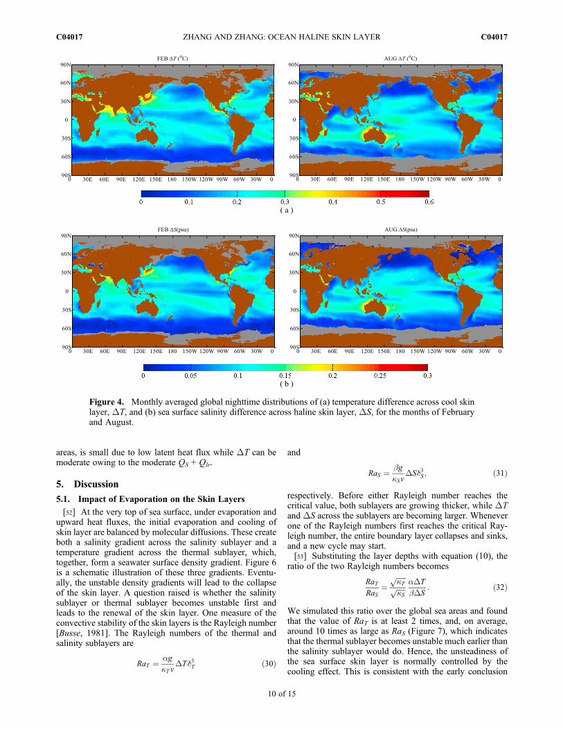
areas, is small due to low latent heat flux while DT can bemoderate owing to the moderate QS + Qlr.

5. Discussion

5.1. Impact of Evaporation on the Skin Layers

[52] At the very top of sea surface, under evaporation andupward heat fluxes, the initial evaporation and cooling ofskin layer are balanced by molecular diffusions. These createboth a salinity gradient across the salinity sublayer and atemperature gradient across the thermal sublayer, which,together, form a seawater surface density gradient. Figure 6is a schematic illustration of these three gradients. Eventu-ally, the unstable density gradients will lead to the collapseof the skin layer. A question raised is whether the salinitysublayer or thermal sublayer becomes unstable first andleads to the renewal of the skin layer. One measure of theconvective stability of the skin layers is the Rayleigh number[Busse, 1981]. The Rayleigh numbers of the thermal andsalinity sublayers are

RaT ¼ agkT v

DTd3T ð30Þ

and

RaS ¼ bgkSv

DSd3S ; ð31Þ

respectively. Before either Rayleigh number reaches thecritical value, both sublayers are growing thicker, while DTand DS across the sublayers are becoming larger. Wheneverone of the Rayleigh numbers first reaches the critical Ray-leigh number, the entire boundary layer collapses and sinks,and a new cycle may start.[53] Substituting the layer depths with equation (10), the

ratio of the two Rayleigh numbers becomes

RaTRaS

¼ffiffiffiffiffiffikT

pffiffiffiffiffikS

p aDT

bDS: ð32Þ

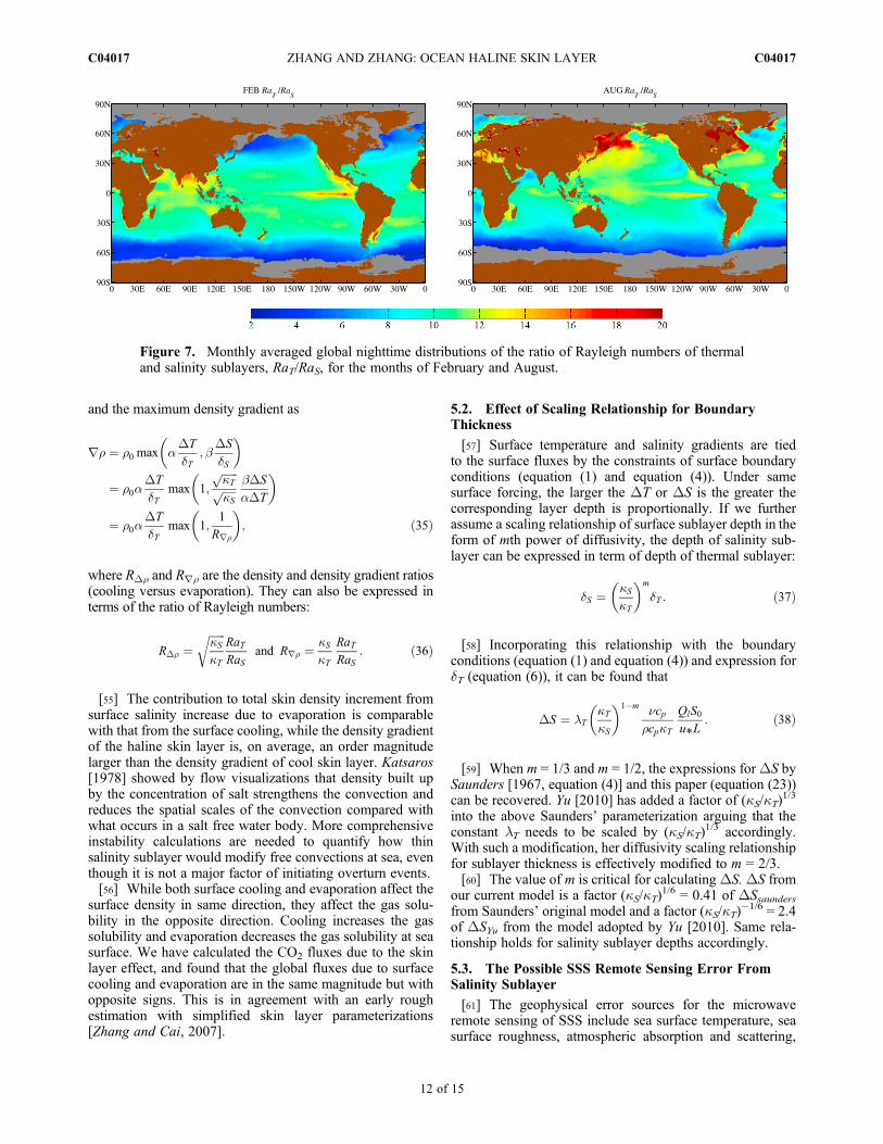
We simulated this ratio over the global sea areas and foundthat the value of RaT is at least 2 times, and, on average,around 10 times as large as RaS (Figure 7), which indicatesthat the thermal sublayer becomes unstable much earlier thanthe salinity sublayer would do. Hence, the unsteadiness ofthe sea surface skin layer is normally controlled by thecooling effect. This is consistent with the early conclusion

Figure 4. Monthly averaged global nighttime distributions of (a) temperature difference across cool skinlayer, DT, and (b) sea surface salinity difference across haline skin layer, DS, for the months of Februaryand August.


10 of 15

from laboratory observations by Katsaros [1969] that thereis an enormous difference in the overturning time scalesbetween thermal and salinity sublayers. The ratio of thecritical overturning time scales of thermal and salinity

sublayers, tcrT and tcr

S , can be found as a function of the ratioof the Rayleigh numbers:

tTcrtScr

¼ bgEagQ0

rcp

!32

¼ RaSRaT

� �32

: ð33Þ

The critical overturning time scale of the salinity sublayer is,therefore, at least 2.8 and, on an average, 31 times as large asthe critical overturning time scale of the thermal sublayer.The critical salt gradient would not be realized on the seasurface normally. Exceptions can occur, for example, wheninfrared absorption under strong solar radiation of day timelargely offsets the surface heat lost to the atmosphere.[54] However, surface evaporation can contribute to the

total density and density gradient at sea surface significantly.Whenwe are concerned about the density difference across theskin layers, we find the total density augmentation to be as

Dr ¼ r0 aDT þ bDSð Þ ¼ r0aDT 1þ bDS

aDT

� �

¼ r0aDT 1þ 1

RDr

� �ð34Þ

Figure 6. Schematic illustrations of profiles of temperature(T(z)), salinity (S(z)), and density (r(z)), within sea surfaceskin layers. The depths of thermal and salinity sublayersare dT and dS, respectively. The lower boundary of the vis-cosity sublayer is too far away to be shown.

Figure 5. Monthly averaged global distributions of (a) sum of sensible heat flux and long wave radiation.Upward fluxes are positive. (b) Ratio of (Qs + Qlr)/Ql for the months of February and August.


11 of 15

and the maximum density gradient as

rr ¼ r0 max aDT

dT;b

DS

dS

� �

¼ r0aDT

dTmax 1;

ffiffiffiffiffiffikT

pffiffiffiffiffikS

p bDS

aDT

� �

¼ r0aDT

dTmax 1;

1

Rrr

� �; ð35Þ

where RDr and Rrr are the density and density gradient ratios(cooling versus evaporation). They can also be expressed interms of the ratio of Rayleigh numbers:

RDr ¼ffiffiffiffiffiffikS

kT

rRaTRaS

and Rrr ¼ kS

kT

RaTRaS

: ð36Þ

[55] The contribution to total skin density increment fromsurface salinity increase due to evaporation is comparablewith that from the surface cooling, while the density gradientof the haline skin layer is, on average, an order magnitudelarger than the density gradient of cool skin layer. Katsaros[1978] showed by flow visualizations that density built upby the concentration of salt strengthens the convection andreduces the spatial scales of the convection compared withwhat occurs in a salt free water body. More comprehensiveinstability calculations are needed to quantify how thinsalinity sublayer would modify free convections at sea, eventhough it is not a major factor of initiating overturn events.[56] While both surface cooling and evaporation affect the

surface density in same direction, they affect the gas solu-bility in the opposite direction. Cooling increases the gassolubility and evaporation decreases the gas solubility at seasurface. We have calculated the CO2 fluxes due to the skinlayer effect, and found that the global fluxes due to surfacecooling and evaporation are in the same magnitude but withopposite signs. This is in agreement with an early roughestimation with simplified skin layer parameterizations[Zhang and Cai, 2007].

5.2. Effect of Scaling Relationship for BoundaryThickness

[57] Surface temperature and salinity gradients are tiedto the surface fluxes by the constraints of surface boundaryconditions (equation (1) and equation (4)). Under samesurface forcing, the larger the DT or DS is the greater thecorresponding layer depth is proportionally. If we furtherassume a scaling relationship of surface sublayer depth in theform of mth power of diffusivity, the depth of salinity sub-layer can be expressed in term of depth of thermal sublayer:

dS ¼ kS

kT

� �m

dT : ð37Þ

[58] Incorporating this relationship with the boundaryconditions (equation (1) and equation (4)) and expression fordT (equation (6)), it can be found that

DS ¼ lTkT

kS

� �1�m ncprcpkT

QlS0u*L

: ð38Þ

[59] When m = 1/3 and m = 1/2, the expressions forDS bySaunders [1967, equation (4)] and this paper (equation (23))can be recovered. Yu [2010] has added a factor of (kS/kT)

1/3

into the above Saunders’ parameterization arguing that theconstant lT needs to be scaled by (kS/kT)

1/3 accordingly.With such a modification, her diffusivity scaling relationshipfor sublayer thickness is effectively modified to m = 2/3.[60] The value of m is critical for calculating DS.DS from

our current model is a factor (kS/kT)1/6 = 0.41 of DSsaunders

from Saunders’ original model and a factor (kS/kT)�1/6 = 2.4

of DSYu from the model adopted by Yu [2010]. Same rela-tionship holds for salinity sublayer depths accordingly.

5.3. The Possible SSS Remote Sensing Error FromSalinity Sublayer

[61] The geophysical error sources for the microwaveremote sensing of SSS include sea surface temperature, seasurface roughness, atmospheric absorption and scattering,

Figure 7. Monthly averaged global nighttime distributions of the ratio of Rayleigh numbers of thermaland salinity sublayers, RaT/RaS, for the months of February and August.


12 of 15

Faraday rotation, and solar and galactic radio emission [Yuehet al., 2001]. The estimated errors contributing from thesefactors are given by Koblinsky et al. [2003]. Among them,the largest error is from the sea surface roughness with avalue of 0.27 psu, while the second and third leading errors,from dry air and cloud liquid water, are 0.13 psu and 0.07psu respectively.[62] Two recent satellite remote sensing projects have

targeted an accuracy of 0.1–0.2 psu on a monthly basis witha spatial resolution of 100–200 km [Koblinsky et al., 2003;Le Vine et al., 2007; Jordà and Gomis, 2010]. In theseprojects, several errors, such as the ones from galactic, sur-face roughness (e.g., waves), Faraday rotation, and solarreflection are reduced [Koblinsky et al., 2003]. The errorscaused by Faraday rotation and solar reflection are respec-tively 0.04 and 0.01 psu.[63] Figure 8 shows the longitudinal averaged monthly

mean DS together with its standard variation for the monthsof February and August. DS at the latitudes between 30�Nand 30�S, is kept around 0.11 psu. At the latitudes higherthan 30�, DS decrease with increasing latitude up to 50�.The rest months of a year share the similar feature with thesetwo months. The averagedDS at low latitudes is about 0.1 to0.13 psu, while the salinity sublayer thickness at the latitudesbetween 30�N and 30�S is mostly thinner than 0.1 mm. Themicrowave penetration depth is about 9 mm when SST =20�C and SSS = 36‰ [Swift, 1980]. The remote sensingerror caused by sea surface salinity sublayer is estimated tobe less than 0.01 psu and negligible at night, even thoughboth thickness of haline layer and salinity increment acrossare found here to be greater than the early global simula-tions. Thicker haline diffusive layer may be reached in warmskin layer situations of daytime and is not included in thecalculations here.

5.4. Surfactant Effect

[64] Surfactant is known to reduce surface tension, elas-ticity, and viscosity [Liu and Duncan, 2003]. The existenceof surface films on ocean surface can affect surfacedynamics. Longitudinal capillary waves of surface filmsdamp the ocean short waves [Alpers and Hühnerfuss, 1989].

Surface films also alter the surface convections [Sayloret al., 2001]. In our calculations, the effects of surfactanton skin layers are not considered and therefore not valid forcoastal zones.

6. Conclusions

[65] We revisited the sea surface skin layer problem on theverge of remote sensing SSS data becoming available. Ourdiscussions are based on a unified model for depths of theskin layers proposed here. We have argued that, since thecharacteristic surface layer depth is resulted from the balancebetween molecular diffusion and frequent disruptions byconvective collapse of the skin layer, by breaking waves,and by small-scale turbulence from below the layer, a con-ceptual analogy to the mixing of scalar quantities in a tur-bulent flow can be applied. The arguments only hold true forthe cases of large Rayleigh number flows when the con-vections become turbulent. It is proposed that the depths ofthe skin layers, such as temperature, salinity, and gas con-centrations, are proportional to the Batchelor micro-scale.We can summarize our findings as the following:[66] 1. By adopting the Batchelor micro-scale, the depths

of sublayers are all proportional to the square root of theirmolecular diffusivities. This diffusivity-dependent relation isconsistent with a wide range of empirical and theoreticalconclusions. Monthly averaged global nighttime distributionof salinity sublayer thickness is simulated. The globallyaveraged thickness of salinity sublayer is found to be about60 mm. The cool skin layer depth is a factor of

ffiffiffiffiffiffiffiffiffiffiffiffiffikT=kS

pthicker, therefore, its global average is slightly under 1 mm.The diffusivity scaling relationship is vital in predicting thedepth of salinity diffusive layer as observations are notreadily available. With a one-third power scaling relation-ship, for example, it is expected a depth of salinity diffusivelayer in the order of 200 mm [Katsaros, 1980].[67] 2. The Richardson number, Ri, introduced to measure

the dominance between free and forced convections, is infact a ratio of time-scales of free and forced convection[Kudryavtsev and Soloviev, 1985]. The turbulent dissipation

Figure 8. Longitudinally averaged DS (solid) and standard variation of DS, and s(DS) (dashed),averaged along the latitudes for the months of February and August.


13 of 15

rate has different relationships with the surface forcingmainly due to the different functional forms of the time-scales. Only limited fraction of ocean surface is dominatedby free convections, i.e., Ri > 1. There is a significant per-centage of low latitude ocean area where Ri < 1 but stillclose to 1. The wave breaking has not been included in thecalculation here. The percentage of area affected by wavebreaking is limited at low to moderate wind speeds. Skinlayers are very weak and not well defined at high windspeeds (highly unstable due to waves).[68] 3. We computed the sea surface salinity difference

DS across the salinity sublayer along with the temperaturedifference DT through the thermal sublayer. Although sim-ilar global distribution patterns of DT and DS are found,there are systematic biases between our results and theresults given by Yu [2010]. At the vicinity of Ri ≈ 1 and thearea of Ri > 1, ourDT is slightly larger when the dependenceof viscosity on temperature is not considered. We take intoconsideration of the effect of seawater viscosity varying withtemperature, which results a reduced DT toward high lati-tudes where water temperature decreases. Our DS is about2.3 times as large as Yu’s, mainly due to the different dif-fusivity scaling relationship used besides the same biases asDT. DS exhibits a similar global pattern with that of DT,except for limited areas at high latitudes. This is due to thesmall variation of S0 and similar global distributions of latentheat flux and total heat flux. It should be noted that the warmlayer effect have not been taken into consideration here, andall calculations are limited to the nighttime condition only.[69] 4. Although DS and the depth of haline skin layer

from our calculations are both greater than the previousresults [Yu, 2010], the thickness of the salinity sublayer isstill much thinner than the electromagnetic depth of pene-tration. For microwave remote sensing of SSS, the error dueto haline skin effect is estimated to be half of the otherleading errors at the most. All calculations are limited to thenighttime condition only. The skin salinity increment andthe depth of salinity sublayers could be doubled under warmlayer daytime conditions. Also, if the model of salinitysublayer was built upon the one-third power law, the maxi-mum error caused by salinity sublayer would be at the sameorder as the leading errors.[70] 5. The ratio of the Rayleigh numbers of thermal and

salinity sublayers is found to be rather large, indicating thatthe convective instability of the skin layer is mainly influ-enced by the unsteadiness of the thermal sublayer rather thanthat of the salinity sublayer. Both cool and haline skin layerscontribute to surface skin density and density gradient, whilethey have opposite effects on gas solubility across the gasconcentration sublayers. Finally, the unified depth modelleads us to a parameterization for gas transfer velocitydirectly through surface under low to moderate winds. Thisparameterization is consistent with prevailing Schmidtnumber scaling law for rough water. Wave breaking is avery signification factor in gas transfer velocity and can beincorporated in by introducing additional criteria as arenewal model by Soloviev and Schlüssel [1994]. Advan-tages of our parameterization are more concise in formulismand clearer in physics. Investigations on the impact of sur-face heat flux on air-sea gas transfer will be reported in aseparate paper.

[71] Acknowledgments. We are indebted to Christopher W. Fairallfor the generosity of supplying COARE data set and to Charles Cox,K. B. Katsaros, and an anonymous reviewer for the helpful comments inpreparing of the final manuscript. Support from the National Science Foun-dation (OCE 0757290 and OCE 0647819), the National Natural ScienceFoundation of China (grant 40776007), and National Science and Technol-ogy Major Projects of China (2009ZX07424–001) is acknowledged. Pro-ducts downloaded from the WHOI OAFlux project and ISCCP are usedin our computations as ocean surface forcing inputs. Y.Z. was supportedby the Lu Foundation of Graduate Education International Exchange, dur-ing working at the Scripps Institution of Oceanography, from September2010 to August 2011.

ReferencesAlpers, W., and H. Hühnerfuss (1989), The damping of ocean waves bysurface films: A new look at an old problem, J. Geophys. Res., 94,6251–6265, doi:10.1029/JC094iC05p06251.

Antonov, J. I., R. A. Locarnini, T. P. Boyer, A. V. Mishonov, and H. E.Garcia (2006), World Ocean Atlas 2005, vol. 2, Salinity, NOAA AtlasNESDIS, vol. 62, edited by S. Levitus, 182 pp., NOAA, Silver Spring,Md.

Batchelor, G. K. (1959), Small-scale variation of convected quantities liketemperature in turbulent fluid: Part 1. General discussion and the caseof small conductivity, J. Fluid Mech., 5, 113–133, doi:10.1017/S002211205900009X.

Brutsaert, W. (1975), The roughness length for water vapor, sensible heat,and other scalars, J. Atmos. Sci., 32, 2028–2031, doi:10.1175/1520-0469(1975)032<2029:TRLFWV>2.0.CO;2.

Busse, F. H. (1981), Transition to turbulence in Rayleigh-Benard convection,in Topics in Applied Physics, vol. 45, Hydrodynamic Instabilities and theTransition to Turbulence, edited by H. L. Swinney and J. P. Gollub,pp. 97–137, Springer, Berlin.

Castro, S. L., G. A. Wick, and W. J. Emery (2003), Further refinements tomodels for the bulk-skin sea surface temperature difference, J. Geophys.Res., 108(C12), 3377, doi:10.1029/2002JC001641.

Coppin, P. A., E. F. Bradley, I. J. Barton, and J. S. Godfrey (1991), Simul-taneous observations of sea surface temperature in the western equatorialPacific Ocean by bulk, radiative, and satellite methods, J. Geophys. Res.,96, 3401–3409.

Danckwerts, P. V. (1951), Significance of liquid-film coefficients in gasabsorption, Eng. Process Dev., 43, 1460–1467.

Fairall, C. W., E. F. Bradley, J. S. Godfrey, G. A. Wick, J. B. Edson, andG. S. Young (1996), Cool-skin and warm-layer effects on sea surfacetemperature, J. Geophys. Res., 101, 1295–1308.

Foster, T. D. (1971), Intermittent convection, Geophys. Fluid Dyn., 2,201–217, doi:10.1080/03091927108236059.

Grassl, H. (1976), The dependence of the measured cool skin of the ocean onwind stress and total heat flux, Boundary Layer Meteorol., 10, 465–474,doi:10.1007/BF00225865.

Handler, R. A., G. B. Smith, and R. L. Leighton (2001), The thermal struc-ture of an air-water interface at low wind speeds, Tellus, Ser. A, 53, 233–244.

Handler, R. A., R. I. Leighton, G. B. Smith, and R. Nagaosa (2003), Surfac-tant effects on passive scalar transport in a fully developed turbulent flow,Int. J. Heat Mass Transfer, 46, 2219–2238, doi:10.1016/S0017-9310(02)00526-4.

Harris, A. R., M. A. Saunders, J. S. Foot, K. F. Smith, and C. T. Mutlow(1995), Improved sea surface temperature retrievals from space, Geophys.Res. Lett., 22, 2159–2162, doi:10.1029/95GL02019.

Hasse, L. (1971), The sea surface temperature deviation and the heat flow atthe sea-air interface, Boundary Layer Meteorol., 1, 368–379,doi:10.1007/BF02186037.

Herring, J. R. (1963), Investigation of problems in thermal convection,J. Atmos. Sci., 20, 325–338, doi:10.1175/1520-0469(1963)020<0325:IOPITC>2.0.CO;2.

Jähne, B., and H. Haußecker (1998), Air-water gas exchange, Annu. Rev.Fluid Mech., 30, 443–468, doi:10.1146/annurev.fluid.30.1.443.

Jähne, B., et al. (1987), On the parameters influencing air-water gasexchange, J. Geophys. Res., 92, 1937–1949, doi:10.1029/JC092iC02p01937.

Jordà, G., and D. Gomis (2010), Accuracy of SMOS level 3 SSS productsrelated to observational errors, IEEE Trans. Geosci. Remote Sens., 48(4),1694–1701, doi:10.1109/TGRS.2009.2034259.

Katsaros, K. B. (1969), Temperature and salinity of the sea surface with par-ticular emphasis on effects of precipitation, Ph.D. thesis, 307 pp., Univ.of Washington, Seattle.

Katsaros, K. B. (1978), Turbulent free convection in fresh and salt water:Some characteristics revealed by visualization, J. Phys. Oceanogr., 8(4),613–626, doi:10.1175/1520-0485(1978)008<0613:TFCIFA>2.0.CO;2.


14 of 15

Katsaros, K. B. (1980), The aqueous thermal boundary layer, BoundaryLayer Meteorol., 18, 107–127, doi:10.1007/BF00117914.

Katsaros, K. B., W. T. Liu, J. A. Businger, and J. E. Tillman (1977), Heattransport and thermal structure in the interfacial boundary layer measuredin an open tank of water in turbulent free convection, J. Fluid Mech.,83(2), 311–335, doi:10.1017/S0022112077001219.

Koblinsky, C. J., P. Hildebrand, D. Levine, F. Pellerano, Y. Chao, W.Wilson,S. Yueh, and G. Lagerloef (2003), Sea surface salinity from space: Sciencegoals and measurement approach, Radio Sci., 38(4), 8064, doi:10.1029/2001RS002584.

Kudryavtsev, V. N., and A. V. Soloviev (1985), On the parameterization ofthe cold film on the ocean surface, Izv. Russ. Acad. Sci. Atmos. OceanicPhys., Engl. Transl., 21, 177–183.

Leighton, R. I., G. B. Smith, and R. A. Handler (2003), Direct numericalsimulations of free convection beneath an air-water interface at lowRayleigh numbers, Phys. Fluids, 15, 3181–3193, doi:10.1063/1.1606679.

Le Vine, D. M., G. S. E. Lagerloef, F. R. Colomb, S. H. Yueh, and F. A.Pellerano (2007), Aquarius: An instrument to monitor sea surface salinityfrom space, IEEE Trans. Geosci. Remote Sens., 45, 2040–2050,doi:10.1109/TGRS.2007.898092.

Liu, W. T., K. B. Katsaros, and J. A. Businger (1979), Bulk parameteriza-tion of air-sea exchange of heat and water vapor including the molecularconstraints at the interface, J. Atmos. Sci., 36, 1722–1735, doi:10.1175/1520-0469(1979)036<1722:BPOASE>2.0.CO;2.

Liu, X., and J. H. Duncan (2003), The effects of surfactants on spillingbreaking waves, Nature, 421, 520–523, doi:10.1038/nature01357.

Paulson, C. A., and T. W. Parker (1972), Cooling of a water surfaceby evaporation, radiation, and heat transfer, J. Geophys. Res., 77(3),491–495, doi:10.1029/JC077i003p00491.

Paulson, C. A., and J. J. Simpson (1981), The temperature difference acrossthe cool skin of the ocean, J. Geophys. Res., 86(C11), 11,044–11,054,doi:10.1029/JC086iC11p11044.

Rapp, R. J., and W. K. Melville (1990), Laboratory measurements of deep-water breaking waves, Philos. Trans. R. Soc. London A, 331, 735–800,doi:10.1098/rsta.1990.0098.

Saunders, P. M. (1967), The temperature at the ocean-air interface,J. Atmos. Sci., 24, 269–273, doi:10.1175/1520-0469(1967)024<0269:TTATOA>2.0.CO;2.

Saylor, J. R., G. B. Smith, and K. A. Flack (2001), An experimental inves-tigation of the surface temperature field during evaporative convection,Phys. Fluids, 13, 428–439, doi:10.1063/1.1337064.

Schlüssel, P., W. J. Emery, H. Grassl, and T. Mammen (1990), On the bulk-skin temperature difference and its impact on satellite remote sensing ofthe sea surface temperature, J. Geophys. Res., 95, 13,341–13,356,doi:10.1029/JC095iC08p13341.

Soloviev, A. V., and P. Schlüssel (1994), Parameterizaiton of the cool skinof the ocean and of the air-ocean gas transfer on the basis of modelingsurface renewal, J. Phys. Oceanogr., 24, 1339–1346, doi:10.1175/1520-0485(1994)024<1339:POTCSO>2.0.CO;2.

Soloviev, A. V., and P. Schlüssel (1996), Evolution of cool skin and directair-sea gas transfer coefficient during daytime, Boundary LayerMeteorol., 77, 45–68, doi:10.1007/BF00121858.

Sverdrup, H. U., M. W. Johnson, and R. H. Fleming (1942), The Oceans:Their Physics, Chemistry, and General Biology, Prentice Hall,New York.

Swift, C. T. (1980), Passive microwave remote sensing of the ocean—A review, Boundary Layer Meteorol., 18, 25–54, doi:10.1007/BF00117909.

Webster, P. J. (1994), The role of hydrological processes in ocean-atmosphereinteractions, Rev. Geophys., 32, 427–476, doi:10.1029/94RG01873.

Wells, A. J., C. Cenedese, J. T. Farrar, and C. J. Zappa (2009), Variations inocean surface temperature due to near-surface flow: Straining the cool skinlayer, J. Phys. Oceanogr., 39, 2685–2710, doi:10.1175/2009JPO3980.1.

Woodcock, A. H., and H. Stommel (1947), Temperatures observed near thesurface of a fresh water pond at night, J. Meteorol., 4, 102–103,doi:10.1175/1520-0469(1947)004<0102:TONTSO>2.0.CO;2.

Yu, L. (2010), On sea surface salinity skin effect induced by evaporationand implications for remote sensing of ocean salinity, J. Phys. Oceanogr.,40, 85–102, doi:10.1175/2009JPO4168.1.

Yu, L., and R. A. Weller (2007), Objectively analyzed air-sea heat fluxesfor the global ice-free oceans (1981–2005): The role of the changing windspeed, J. Clim., 20, 5376–5390, doi:10.1175/2007JCLI1714.1.

Yueh, S. H., R. West, W. Wilson, F. Li, E. Njoku, and Y. Rahmat Samii(2001), Error sources and feasibility for microwave remote sensing ofSSS, IEEE Trans. Geosci. Remote Sens., 39, 1049–1060, doi:10.1109/36.921423.

Zhang, X., and W. J. Cai (2007), On some biases of estimating the globaldistribution of air-sea CO2 flux by bulk parameterizations, Geophys.Res. Lett., 34, L01608, doi:10.1029/2006GL027337.

Zhang, Y., W. B. Rossow, A. A. Lacis, V. Oinas, and M. I. Mishchenko(2004), Calculation of radiative fluxes from the surface to top of atmo-sphere based on ISCCP and other global data sets: Refinements of theradiative transfer model and the input data, J. Geophys. Res., 109,D19105, doi:10.1029/2003JD004457.

X. Zhang, Scripps Institution of Oceanography, University of California,San Diego, La Jolla, CA 92093-0213, USA. ([email protected])Y. Zhang, College of Civil Engineering and Architecture, Zhejiang

University, Hangzhou, Zhejiang 310058, China.


15 of 15

ocean haline skin layer and turbulent surface...

Documents