1

Ocean Ecosystem Indicators of Salmon Marine Survival in the Northern California Current

William T. Peterson,1

Cheryl A. Morgan,2

Jay O. Peterson, 2

Jennifer L. Fisher,2 Brian J. Burke

3

and Kurt Fresh3

1Fish Ecology Division

Northwest Fisheries Science Center National Marine Fisheries Service

Newport Research Station 2032 S Marine Science Drive Newport, Oregon 97365-5275

2Cooperative Institute for Marine Resource Studies

Hatfield Marine Science Center Oregon State University

2030 S Marine Science Drive Newport, Oregon 97365-5257

3Fish Ecology Division

Northwest Fisheries Science Center National Marine Fisheries Service

2725 Montlake Blvd. East Seattle, WA 98112-2097

December 2012

2

Table of Contents

Project Summary ............................................................................................................................. 3 Ocean Ecosystem Indicators of Salmon Marine Survival in the Northern California Current .. 3

Summary of 2012 ocean ecosystem indicators and pre-season outlook for 2013 .......................... 4 Forecast of Adult Returns for coho and Chinook Salmon .............................................................. 8 Adult Returns of Chinook and Coho Salmon ............................................................................... 16 Large–scale Ocean and Atmospheric Indicators ........................................................................... 19

Pacific Decadal Oscillation (PDO) ........................................................................................... 19 Oceanic Niño Index (ONI) ....................................................................................................... 22

Local and Regional Physical Indicators ........................................................................................ 25 Temperature Anomalies ........................................................................................................... 25 Coastal Upwelling .................................................................................................................... 28 Hypoxia .................................................................................................................................... 33 Physical Spring Transition ....................................................................................................... 34 Deep–Water Temperature and Salinity .................................................................................... 37

Local Biological Indicators ........................................................................................................... 41 Copepod Biodiversity ............................................................................................................... 41 Northern and Southern Copepod Anomalies ............................................................................ 47 Copepod Community Structure ................................................................................................ 52 Biological Spring Transition .................................................................................................... 55 Winter Ichthyoplankton ............................................................................................................ 60 Catches of Yearling Chinook in June and Coho in September ................................................ 64

Indicators Under Development ..................................................................................................... 66 Forage Fish and Pacific Hake Abundance ............................................................................... 66 A Second Mode of North Pacific Sea Surface Temperature Variation .................................... 68 Phytoplankton Biomass ............................................................................................................ 69 Euphausiid Egg Concentration and Adult Biomass ................................................................. 69 Interannual Variations in Habitat Area .................................................................................... 69 Salmon Predation Index ........................................................................................................... 70 Potential Indices for Future Development ................................................................................ 70

Ocean Sampling Methods ............................................................................................................. 71 Hydrography, Zooplankton, and Ichthyoplankton ................................................................... 71 Juvenile Salmon Sampling Program ........................................................................................ 73

Introduction to Pacific Northwest Oceanography......................................................................... 77 Physical Oceanographic Considerations .................................................................................. 77 Climate–Scale Physical Variability .......................................................................................... 79

Acknowledgments......................................................................................................................... 82 References ..................................................................................................................................... 83 Glossary ........................................................................................................................................ 87

3

Project Summary

Ocean Ecosystem Indicators of Salmon Marine Survival in the Northern California Current

As many scientists and salmon managers have noted, variations in marine survival of salmon often correspond with periods of alternating cold and warm ocean conditions. For example, cold conditions are generally good for Chinook and coho salmon, whereas warm conditions are not.

These pages are based on our website of how physical and biological ocean conditions may affect the growth and survival of juvenile salmon in the northern California Current off Oregon and Washington. We present a number of physical, biological, and ecosystem indicators to specifically define the term "ocean conditions." More importantly, these metrics can be used to forecast the survival of salmon 1–2 years in advance, as shown in Table 1. This information is presented for the non–specialist; additional detail is provided via links when possible.

Material presented in this report has two sources. One is the World Wide Web, from which we have drawn values for the Pacific Decadal Oscillation, Multivariate ENSO index, Upwelling Index, and sea surface temperatures. Links and references to these sources are given in the respective sections that deal with these four physical variables. All other data are from our direct observations during a) biweekly oceanographic sampling along the Newport Hydrographic Line and b) annual juvenile salmonid surveys conducted in June and September. Survey station locations are shown in Figure 1; sampling and survey methods are presented in "Ocean Sampling Methods."

Using all of these data, we developed a suite of ocean ecosystem indicators upon which to base forecasts of salmon returns. These forecasts are presented as a practical example of

Figure 1. Transects sampled during trawling surveys off the coast of Oregon and Washington.

4

how ocean ecosystem indicators can be used to inform management

decisions for endangered salmon. At this time, the forecasts are qualitative in nature: we rate each in terms of its "good," "bad," or "neutral" relative impact on salmon marine survival (Table 1).

We use this suite of indicators to complement existing indicators used to predict adult salmon runs, such as jack returns, smolt–to–adult return rates (Scheuerell and Williams 2005), and the Logerwell production index.

The strength of this approach is that biological indicators are directly linked to the success of salmon during their first year at sea through food–chain processes. These biological indicators, coupled with physical oceanographic data, offer new insight into the mechanisms that lead to success or failure for salmon runs.

In addition to forecasting salmon returns, the indicators presented here may be of use to those trying to understand how variations in ocean conditions might affect recruitment of fish stocks, seabirds, and other marine animals. We reiterate that trends in salmon survival track regime shifts in the North Pacific Ocean, and that these shifts are transmitted up the food chain in a more–or–less linear and bottom–up fashion as follows:

upwelling → nutrients → plankton → forage fish → salmon.

The same regime shifts that affect Pacific salmon also affect the migration of Pacific hake and the abundance of sea birds, both of which prey on migrating juvenile salmon. Therefore, climate variability can also have "top down" impacts on salmon through predation by hake and sea birds (terns and cormorants). Both "bottom up" and "top down" linkages are explored here.

Summary of 2012 ocean ecosystem indicators and pre-season outlook for 2013

The Pacific Decadal Oscillation (PDO) has been negative and cold ocean conditions have prevailed for most of the period between September 2007 through 2012. This was interrupted by a brief moderate El Niño event from Aug 2009-May 2010, but otherwise the PDO has been strongly negative over a period of more than five years. If the PDO were the only indicator of "ocean conditions" for the northern California Current, this situation would be worthy of praise. However, local conditions did not mirror the PDO in 2012; the date of spring transition (from winter downwelling conditions to summer upwelling) was very late – it did not occur until 2 May, three weeks later than the long-term average. Moreover, winds were light and variable through May and June, and sea surface temperature values were several degrees warmer than ‘normal’ from mid–June through July. The significance of these observations is two–fold:

• The PDO alone does not reflect local conditions because values during much of 2012 were among the most negative of any in the past 100 years, yet sea surface temperatures were elevated;

5

• Very warm surface water in June and July was almost certainly harmful to juvenile salmon which entered the sea in May because elevated temperatures will result in increased metabolism and likely poor feeding conditions.

This suggests that the early summer period of 2012 was a time of poor ocean conditions from the viewpoint of those taxa of juvenile salmon that live locally. However, fish such as juvenile Snake River spring (stream-type; yearling) Chinook salmon that migrate out of the area quickly may have migrated northwards and left the area before poor conditions prevailed.

A final comment is that an El Niño is brewing at the equator with all equatorial indices in the “positive” range. However, at the time of this writing (mid-December 2012), “El Niño neutral” conditions exist.

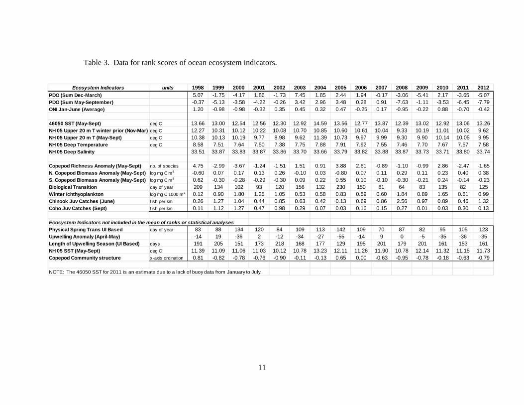
Next we discuss the state of each of our ecological indicators of ocean conditions in the context of how our measurements in 2012 compared to those made by our research team since 1998. Annual values for each indicator from 1998 until present are listed in Table 3.

Pacific Decadal Oscillation—The PDO was strongly negative through 2012, reaching a value of -2.21 in September (Figure 5). The most recent value available (-0.59, for November) suggests that the negative phase is weakening.

The Oceanic Niño Index (ONI)—The ONI values have been steadily increasing since December 2011 and have been positive since June 2012; as of November 2012 the ONI index was + 0.8 suggesting “El Niño conditions”, however the NOAA Climate Prediction Center’s website, http://www.cpc.ncep.noaa.gov/products/analysis_monitoring/enso_advisory/ensodisc.pdf, states that it is considered unlikely that a fully coupled El Niño will develop during the next several months. ENSO-neutral is now favored through the Northern Hemisphere winter 2012-13 and into spring 2013.

Sea Surface Temperature (SST)—At the NOAA Buoy 46050, 20 miles offshore of Newport, SST usually tracks the PDO closely, however this was not the case during the summer of 2012 (Figure 5). Daily values of SST (Figure 6), show positive (warm) temperature anomalies in June and July, with daily values of temperature anomalies around +3°C in mid-July. The monthly average anomaly was + 1.7°C for July, at a time when the PDO value was – 1.52. Thus, we issue a warning -- although the PDO usually tracks local conditions, this was not the case during summer 2012. SST at one of our baseline hydrographic stations (NH05, five miles offshore of Newport) was also above-average over the May-September period (Figure 7), with a peak in SST (15.9°C) observed on 25 June, a value which was the 12th warmest of 450 measurements made at this location since 1996.

Mixed Layer Temperatures (MLT). —Mixed Layer Temperatures refer to temperatures averaged over the upper 20 m of the water column, that part of the water column that is mixed by the wind in summer. When these values are calculated, we learned that despite warm sea surface temperatures in 2012 (and 2007 and 2009), when the mixed layer temperatures are compared, anomalies during the upwelling season were below average (i.e., cooler than ‘normal’) for the

6

past seven years (Figure 7). Winter MLTs however were the same as winter SST (Figure 7), likely because the entire water column is well-mixed by intense winter storms. These observations create a problem for interpreting ocean conditions. SST values are readily available from satellite and buoy measurements, but do they adequately represent habitat conditions for juvenile salmon, or is the MLT more representative? We know for certain that they live in the upper parts of the water column in depths < 20 m, but exactly where in the upper layer, and for how long, is not known with certainty.

Coastal Upwelling.—Upwelling was initiated on 2 May and ended on 12 October. The duration was 161 days (Figure 11), ranking 11th out of 15 years. The start date was three weeks later than the long-term average; however, after only a few days, upwelling ceased and did not resume until early July, after which the upwelling index pointed towards strong and nearly continuous upwelling, with only brief pauses, until October. However as shown above, very warm surface water was found on the continental shelf on nearly all days in July (at a time when the upwelling index was suggesting strong upwelling). Thus, the UI did not index local conditions during the summer of 2012. Since the UI is a large-scale indicator (as is the PDO), we wonder what kinds of atmospheric events occurred locally and caused these two basin-scale indicators to fail to index local conditions.

Deep Water Temperature and Salinity—The year 2012 saw the continuation of a trend that began in 2009 towards slightly warmer and fresher water at depth on the continental shelf. We take this as an indication that upwelling has been weak and the source of the waters which upwell are from a shallower depth offshore. The April-June 2012 data Figure 17 were among the fresher and warmer years; July-September was cool and fresh (often referred to as ‘minty’ water). This is reflected in the sea surface temperature data as well – warmer waters prevailed through much of 2012.

Copepod Biodiversity (Species Richness)—Species richness is the number of copepod species in plankton samples. Monthly averaged values of copepod species composition continue to track the PDO quite closely Figure 21; the average for the upwelling season (May-September) in 2012 was ~ 9 species, the same as observed from 2007-2009 and in 2011, but higher than during the cool period of 2000-2001 when the average was about 7 species (Figure 23).

Northern Copepod Anomalies—Copepods are transported to the Oregon coast, either from the north/northwest or from the west/south. Copepods that arrive from the north are cold–water species that originate from the coastal Gulf of Alaska; these are referred to as the "northern copepods." The "northern copepod index" is the log biomass anomaly of three species of cold–water copepods: Calanus marshallae, Pseudocalanus mimus, and Acartia longiremis. This index tracks closely with the PDO (Figure 24). This index was especially significant in summer 2011 and 2012 because the log of the northern copepod biomass anomaly during these two years was the highest we have seen (Table 2 and 3). Further, we experienced a relatively cool winter/spring starting in late 2011, with strongly negative PDO values, and correspondingly the biomass of northern copepods was much higher than average (Figure 24). The high biomass of northern copepods observed in 2011, and persisting into winter and through the summer 2012, is indicative of very good ocean conditions.

7

Biological Spring Transition—The biological spring transition is defined as the date when the zooplankton community has transitioned from a warm–water "winter" community to a cold–water"summer" community. During 2012, the biological transition occurred on day 125 (4 May), as shown in Table 3. May 8th is the median date of transition, so 2012 was about average. However, it was ranked fourth out of the 15 years so this is an indication of fair ocean conditions. Several methods are used to calculate dates of the spring and fall transition, and a compilation of the different methods (including our “biological transition”) is available from Columbia River DART (Data Access in Real Time), a project of the University of Washington School of Aquatic and Fishery Sciences (http://www.cbr.washington.edu/data/trans.html).

Winter Ichthyoplankton—Annual abundance estimates of key salmon prey in winter and early spring provide an indicator of survival in the months before juvenile salmon enter the sea because these estimates reflect the feeding conditions they will potentially encounter. Data from January-March 2012 (Table 3) were also ranked sixth out of the 15 years, indicating average feeding conditions for juvenile salmon that entered the sea in spring 2012 (Figure 34).

Catches of Spring Chinook in June—Pelagic trawl surveys have been carried out for 15 years, since 1998. In recent June surveys (2008 & 2009) catches of spring Chinook salmon have been high, with record high catches in 2008. Although, catches in June 2011 were poor, catches in June 2012 were high, ranking 2nd among the 15 years of surveys (Figure 36).

Catches of Coho in September—Catches of juvenile coho salmon in our September trawl surveys have been a fairly good indicator of rates of return of coho salmon the following year (Figure 37). ). Catches in September 2011 were high, however catches of juvenile coho salmon in the September 2012 survey were relatively low and ranked 10th out of the 15 years (Figure 36).

Overall Summary

1. Positive Signals in 2012: o PDO and ONI strongly negative during winter 2012; o Ocean was colder than normal by 1°C during winter, the 2nd coldest value in 17

years. o Northern copepod biomass was the highest in 17 years and the copepod

community composition index, the 4th highest. o Winter ichthyoplankton biomass had a rank of 6, slightly above average

2. Negative signals: o Despite good local ocean conditions in winter, upwelling was delayed by three

weeks from its normal start date to the first week of May – shown by both the upwelling index (physical transition was on 2 May) and the copepod index (biological transition was 4 May).

o The cumulative upwelling index showed that even though upwelling began on 2 May, winds remained light and variable such that significant amounts of upwelling did not occur until early July. Furthermore, sea surface temperatures remained anomalously high in July, averaging about 2°C above normal. This condition may have been unfavorable for those taxa of juvenile salmon which live

8

in the surface layers of the ocean because these temperatures would have significantly elevated their metabolism, requiring them to feed at higher rates. However, the average temperatures for the upper mixed layer were average.

o On the other hand, spring Chinook salmon catches in our June surveys were the second highest in 15 years. These fish migrate northwards quickly en route to the coastal Gulf of Alaska, and by June are at the northern end of our survey area (and already off Vancouver Island) thus they may not have experienced the warm temperatures which first appeared on 15 June. Coho salmon on the other hand (which are more resident in local waters) would have experienced high SST throughout much of summer which may explain why catches in September were poor, ranking 10th of 15 years.

When all of the indicators are taken as a whole (Table 2), the year 2012 has a rank 4 out of 15, suggesting above-average returns of coho in 2013 and Chinook in 2014. (Note that we now exclude the "upwelling indicators" from the average rankings, but all values are shown in Table 3).

Similar to the past several years, individual indicators have sent a mixed message. Certain indicators suggest the potential for above average returns: persistence of strong La Niña conditions, a negative PDO, positive copepod indicators from May-September, and high catches of spring Chinook salmon in the June survey. However, negative indicators include a late start to the upwelling season (first week of May), nearly a two month delay until upwelling became strong (not until early July), and very warm sea surface temperatures in June and July. The upwelling season was among the shorter ones, only 161 days (as compared to more than 200 days in 1999, 2002, and 2009). Because of these mixed signals, we are less certain of our prediction for coho salmon in 2013 and Chinook salmon in 2014, a statement that we made last year as well.

Forecast of Adult Returns for coho and Chinook Salmon

2012 was characterized by a steady move from La Niña conditions towards an ENSO-neutral state. Combined with persistently negative PDO values throughout the year, a high biomass of lipid-rich northern copepods supporting the base of the food-chain, and an above average abundance of winter-time ichthyoplankton (larval stages of fish-prey for salmon), 2012 had the potential to be a good year for supporting juvenile salmon entering the ocean. This positive bio-physical outlook was tempered a bit by a late start to upwelling, warm sea-surface temperatures through much of the summer, and a trend towards El Niño conditions, but overall the ocean conditions in 2012 appear to be greatly improved compared to the last several years.

Our annual update of ecosystem indicators during 2012 is here, and our "stoplight" rankings and predictions are shown below in Table 1, Table 2, and Figure A.

Table 1. Ocean ecosystem indicators of the Northern California Current. Colored squares indicate positive (green), neutral (yellow), or negative (red) conditions for salmon entering the ocean each year. In the two columns to the far right, colored dots

9

indicate the forecast of adult returns based on ocean conditions in 2012.

Juvenile Migration Year Outlook

2009

2010

2011

2012 Coho 2013

Chinook 2014

Large– scale ocean and atmospheric indicators PDO (May — Sept) ■ ■ ■ ■ ● ●

ONI (Jan-Jun) ■ ■ ■ ■ ● ● Local and regional physical indicators

Sea surface temperature anomalies

■ ■ ■ ■ ● ●

Coastal upwelling ■ ■ ■ ■ ● ● Physical spring

transition

■ ■ ■ ■ ● ●

Deep water temperature and salinity

■ ■ ■ ■ ● ●

Local biological indicators Copepod biodiversity ■ ■ ■ ■ ● ●

Northern copepod anomalies

■ ■ ■ ■ ● ●

Biological spring transition

■ ■ ■ ■ ● ●

Spring Chinook––June ■ ■ ■ ■ -- ● Coho––September ■ ■ ■ ■ ● --

Key ■ good conditions for salmon ● good returns expected

■ intermediate conditions for salmon -- no data

■ poor conditions for salmon ● poor returns expected

Table 2 shows rank scores for the color-coding in Table 1. Scores were assigned based on their effect on juvenile salmonids. We show variables that are correlated with returns of coho salmon after 1 year and of Chinook salmon after 2 years. For example, positive PDO values (and red colors) indicate poor ocean conditions in coastal waters off the northern California Current. Similarly, higher sea surface temperatures in summer are a negative indicator for salmon, but particularly so for resident coho. Table 3 shows the values of each variable shown by rank in Table 2.

10

Table 2. Rank scores upon which color-coding of ocean ecosystem indicators is based. Lower numbers indicate better

ocean ecosystem conditions, or "green lights" for salmon growth and survival, with ranks 1-4 green, 5-10 yellow, and 11-14 red. To arrive at these rank scores, 14 years of sampling data were compared across years (within each row), and each year received a rank between 1 and 14.

Ecosystem Indicators 1998 1999 2000 2001 2002 2003 2004 2005 2006 2007 2008 2009 2010 2011 2012

PDO (December-March) 14 6 3 10 7 15 9 13 11 8 5 1 12 4 2PDO (May-September) 9 4 6 5 10 14 13 15 11 12 2 8 7 3 1ONI Jan-June 15 1 1 6 11 12 10 13 7 9 3 8 14 4 5

46050 SST (May-Sept) 13 8 3 4 1 7 15 12 5 14 2 9 6 10 11NH 05 Upper 20 m T winter prior (Nov-Mar) 15 9 6 8 5 12 13 10 11 4 1 7 14 3 2NH 05 Upper 20 m T (May-Sept) 13 10 12 4 1 3 15 14 7 8 2 5 11 9 6NH 05 Deep Temperature 15 4 8 3 1 11 12 13 14 5 2 10 9 6 7NH 05 Deep Salinity 15 3 6 2 5 13 14 9 7 1 4 11 12 8 10

Copepod Richness Anomaly 15 2 1 6 5 11 10 14 12 9 7 8 13 3 4N. Copepod Biomass Anomaly 14 10 6 7 4 13 12 15 11 9 3 8 5 1 2S. Copepod Biomass Anomaly 15 3 5 4 2 10 12 14 11 9 1 7 13 8 6Biological Transition 14 10 6 5 7 13 9 15 12 2 1 4 11 3 8Winter Ichthyoplankton 15 7 2 4 5 14 13 9 12 11 1 8 3 10 6Chinook Juv Catches (June) 14 3 4 12 8 10 13 15 9 7 1 5 6 11 2Coho Juv Catches (Sept) 11 2 1 4 3 6 12 14 8 9 7 15 13 5 10

Mean of Ranks 13.8 5.5 4.7 5.6 5.0 10.9 12.1 13.0 9.9 7.8 2.8 7.6 9.9 5.9 5.5RANK of the Mean Rank 15 4 2 6 3 12 13 14 10 9 1 8 11 7 4Principle Component Scores (PC1) 6.56 -2.22 -2.95 -1.60 -2.12 2.08 3.12 4.21 1.10 -0.30 -4.39 -0.91 1.13 -1.76 -1.96Principle Component Scores (PC2) -0.51 0.04 -0.24 -0.76 -1.96 -1.53 2.55 -0.43 -0.66 1.07 -0.50 0.96 -0.74 1.36 1.35

Ecosystem Indicators not included in the mean of ranks or statistical analysesPhysical Spring Trans (UI Based) 3 6 14 12 4 9 11 15 9 1 5 2 7 8 13Upwelling Anomaly (Apr-May) 7 1 13 3 6 10 9 15 7 2 4 5 11 13 11Length of Upwelling Season (UI Based) 6 2 14 9 1 10 8 15 5 3 7 3 11 13 11NH 05 SST (May-Sept) 10 6 5 4 1 3 15 13 8 12 2 14 9 7 11Copepod Community Structure 15 3 5 7 2 12 11 14 13 8 1 6 10 9 4

11

Table 3. Data for rank scores of ocean ecosystem indicators.

Ecosystem Indicators units 1998 1999 2000 2001 2002 2003 2004 2005 2006 2007 2008 2009 2010 2011 2012

PDO (Sum Dec-March) 5.07 -1.75 -4.17 1.86 -1.73 7.45 1.85 2.44 1.94 -0.17 -3.06 -5.41 2.17 -3.65 -5.07PDO (Sum May-September) -0.37 -5.13 -3.58 -4.22 -0.26 3.42 2.96 3.48 0.28 0.91 -7.63 -1.11 -3.53 -6.45 -7.79ONI Jan-June (Average) 1.20 -0.98 -0.98 -0.32 0.35 0.45 0.32 0.47 -0.25 0.17 -0.95 -0.22 0.88 -0.70 -0.42

46050 SST (May-Sept) deg C 13.66 13.00 12.54 12.56 12.30 12.92 14.59 13.56 12.77 13.87 12.39 13.02 12.92 13.06 13.26NH 05 Upper 20 m T winter prior (Nov-Mar) deg C 12.27 10.31 10.12 10.22 10.08 10.70 10.85 10.60 10.61 10.04 9.33 10.19 11.01 10.02 9.62NH 05 Upper 20 m T (May-Sept) deg C 10.38 10.13 10.19 9.77 8.98 9.62 11.39 10.73 9.97 9.99 9.30 9.90 10.14 10.05 9.95NH 05 Deep Temperature deg C 8.58 7.51 7.64 7.50 7.38 7.75 7.88 7.91 7.92 7.55 7.46 7.70 7.67 7.57 7.58NH 05 Deep Salinity 33.51 33.87 33.83 33.87 33.86 33.70 33.66 33.79 33.82 33.88 33.87 33.73 33.71 33.80 33.74

Copepod Richness Anomaly (May-Sept) no. of species 4.75 -2.99 -3.67 -1.24 -1.51 1.51 0.91 3.88 2.61 -0.89 -1.10 -0.99 2.86 -2.47 -1.65N. Copepod Biomass Anomaly (May-Sept) log mg C m-3 -0.60 0.07 0.17 0.13 0.26 -0.10 0.03 -0.80 0.07 0.11 0.29 0.11 0.23 0.40 0.38S. Copepod Biomass Anomaly (May-Sept) log mg C m-3 0.62 -0.30 -0.28 -0.29 -0.30 0.09 0.22 0.55 0.10 -0.10 -0.30 -0.21 0.24 -0.14 -0.23Biological Transition day of year 209 134 102 93 120 156 132 230 150 81 64 83 135 82 125Winter Ichthyoplankton log mg C 1000 m-3 0.12 0.90 1.80 1.25 1.05 0.53 0.58 0.83 0.59 0.60 1.84 0.89 1.65 0.61 0.99Chinook Juv Catches (June) f ish per km 0.26 1.27 1.04 0.44 0.85 0.63 0.42 0.13 0.69 0.86 2.56 0.97 0.89 0.46 1.32Coho Juv Catches (Sept) f ish per km 0.11 1.12 1.27 0.47 0.98 0.29 0.07 0.03 0.16 0.15 0.27 0.01 0.03 0.30 0.13

Ecosystem Indicators not included in the mean of ranks or statistical analysesPhysical Spring Trans UI Based day of year 83 88 134 120 84 109 113 142 109 70 87 82 95 105 123Upwelling Anomaly (April-May) -14 19 -36 2 -12 -34 -27 -55 -14 9 0 -5 -35 -36 -35Length of Upwelling Season (UI Based) days 191 205 151 173 218 168 177 129 195 201 179 201 161 153 161NH 05 SST (May-Sept) deg C 11.39 11.09 11.06 11.03 10.12 10.78 13.23 12.11 11.26 11.90 10.78 12.14 11.32 11.15 11.73Copepod Community structure x-axis ordination 0.81 -0.82 -0.78 -0.76 -0.90 -0.11 -0.13 0.65 0.00 -0.63 -0.95 -0.78 -0.18 -0.63 -0.79

NOTE: The 46050 SST for 2011 is an estimate due to a lack of buoy data from January to July.

12

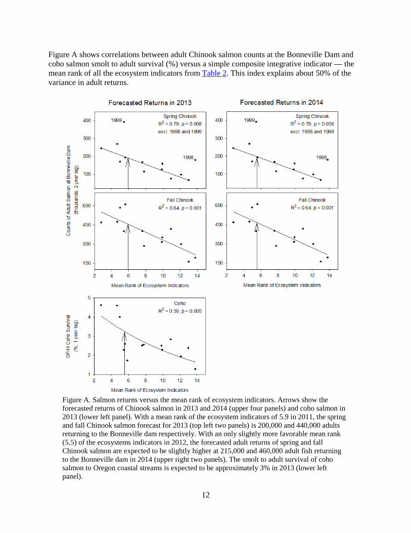
Figure A shows correlations between adult Chinook salmon counts at the Bonneville Dam and coho salmon smolt to adult survival (%) versus a simple composite integrative indicator — the mean rank of all the ecosystem indicators from Table 2. This index explains about 50% of the variance in adult returns.

Figure A. Salmon returns versus the mean rank of ecosystem indicators. Arrows show the forecasted returns of Chinook salmon in 2013 and 2014 (upper four panels) and coho salmon in 2013 (lower left panel). With a mean rank of the ecosystem indicators of 5.9 in 2011, the spring and fall Chinook salmon forecast for 2013 (top left two panels) is 200,000 and 440,000 adults returning to the Bonneville dam respectively. With an only slightly more favorable mean rank (5.5) of the ecosystems indicators in 2012, the forecasted adult returns of spring and fall Chinook salmon are expected to be slightly higher at 215,000 and 460,000 adult fish returning to the Bonneville dam in 2014 (upper right two panels). The smolt to adult survival of coho salmon to Oregon coastal streams is expected to be approximately 3% in 2013 (lower left panel).

13

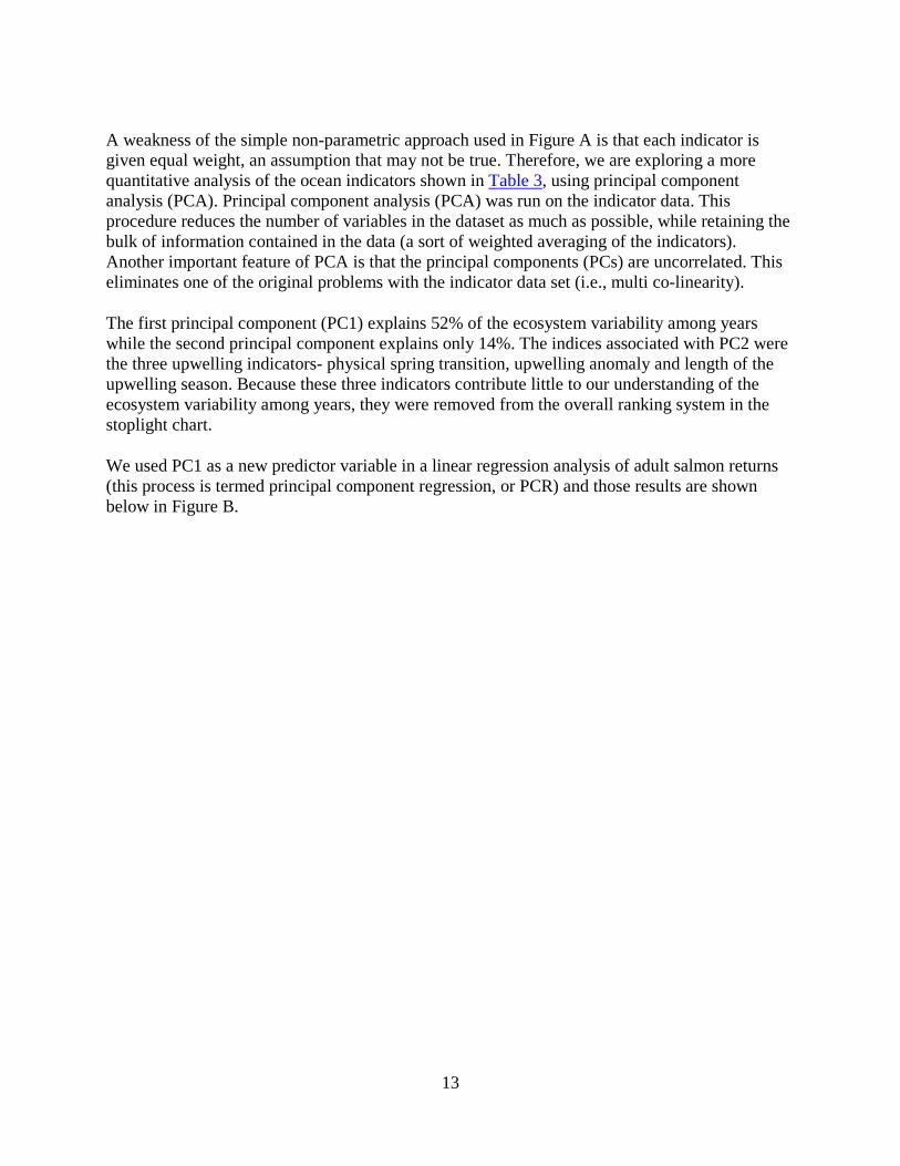
A weakness of the simple non-parametric approach used in Figure A is that each indicator is given equal weight, an assumption that may not be true. Therefore, we are exploring a more quantitative analysis of the ocean indicators shown in Table 3, using principal component analysis (PCA). Principal component analysis (PCA) was run on the indicator data. This procedure reduces the number of variables in the dataset as much as possible, while retaining the bulk of information contained in the data (a sort of weighted averaging of the indicators). Another important feature of PCA is that the principal components (PCs) are uncorrelated. This eliminates one of the original problems with the indicator data set (i.e., multi co-linearity).

The first principal component (PC1) explains 52% of the ecosystem variability among years while the second principal component explains only 14%. The indices associated with PC2 were the three upwelling indicators- physical spring transition, upwelling anomaly and length of the upwelling season. Because these three indicators contribute little to our understanding of the ecosystem variability among years, they were removed from the overall ranking system in the stoplight chart.

We used PC1 as a new predictor variable in a linear regression analysis of adult salmon returns (this process is termed principal component regression, or PCR) and those results are shown below in Figure B.

14

Figure B. Salmon returns versus the first principle axis scores (PC1) from a Principal Component Analysis on the environmental indicators from Table 2.

Although the PCA scores represent a general description of ocean conditions, we must acknowledge that the importance of any particular indicator will vary among salmon species/runs. We are therefore working towards stock-specific salmon forecasts by using methods that can optimally weight the indicators for each response variable in which we are interested (Burke et al. 2013). Figure C compares the actual adult returns of adult yearling Chinook salmon, at three different locations along the Columbia River, to the forecasted returns derived from a maximum covariance analysis (MCA) of the ecosystem indicators. This technique is similar to the principal component regression illustrated in Figure B. We chose these three locations because they roughly represent different salmon populations: Bonneville Dam counts represent all Columbia River spring Chinook salmon, Ice Harbor Dam counts represent

15

Snake River spring/summer Chinook salmon, and Priest Rapids Dam counts represent Upper Columbia River spring Chinook salmon. This is work being conducted by Brian Burke (NWFSC/FE).

Figure C. Time series of estimated adult yearling Chinook salmon returns (blue circles) to the mouth of the Columbia River (count of adults observed at Bonneville Dam plus estimated downstream harvest; top), Ice Harbor Dam (middle), and Priest Rapids Dam (bottom). We used Maximum Covariance Analysis to summarize the indicator data and linear regression to fit the adult return data (orange diamonds) with 95% confidence intervals. We also used the model to predict adult returns in 2013 (purple diamonds) with 95% prediction intervals. The model forecasted that 221,000 adult spring Chinook salmon will return to the Columbia River mouth in 2013, 97,000 will return to Ice Harbor Dam, and 19,500 to Priest Rapids Dam. The x-axis is the smolt out-migration year that corresponds to the year characterized with ecosystem indicators. Results are from work done by Brian Burke (NWFSC/FE).

16

Similar to the past several years, individual indicators have sent a mixed message. Certain indicators suggest the potential for above average returns: i.e. persistence of strong La Niña conditions, a negative PDO, positive copepod indicators from May-September, and high catches of spring Chinook in the June survey. However, negative indicators include a late start to the upwelling season (first week of May), nearly a two month delay until upwelling became strong (not until early July), and very warm sea surface temperatures in June and July. The upwelling season was among the shorter ones, only 161 days (as compared to more than 200 days in 1999, 2002, and 2009). Our best guess is to expect average to above-average returns of coho in 2013 and Chinook in 2014, but similar to the statement we made last year, the mixed signals add greater uncertainty to our predictions.

Adult Returns of Chinook and Coho Salmon

For specific stocks of Chinook and coho salmon, the proportion of adult returns from a particular year class is not often known. This proportion, or escapement, is the number of juvenile salmon that survive to the smolt stage, migrate to the ocean, and return to spawn as adults after several months or years (Healy 1991). .

Ordinarily, the proportions of fish that die in freshwater vs. those that die in the ocean can only be estimated. Thus adult return data, such as counts at dams or traps, can be used only as an index or surrogate measure of ocean survival. With these caveats in mind, we present adult data from various sources with which we compare forecasts based on ocean indicators.

The table below (Table 4) is color-coded according to ranks of adult return data from each year for which we have corresponding ocean indicator data. Adult data are lagged behind ocean entry by 1 year for coho and 2-3 years for spring and fall Chinook salmon; therefore, as of 2012, we have 15 years of indicator data but only 12 - 14 years of adult return data.

17

Table 4. Ranks among years for adult returns by year of ocean entry, 1998-present.

Colors represent high (green), intermediate (yellow) and low (red) returns.

Adult returns by Year of Ocean Entry¹

OPIH Coho

(adults:smolts)

Bonneville spring

Chinook (n)

Bonneville fall

Chinook (n)

Klamath River fall Chinook

(n est.)

1998 14 5 7 2 1999 11 1 3 3 2000 2 2 1 1 2001 5 4 2 8 2002 3 6 5 10 2003 4 12 10 11 2004 12 11 12 4 2005 9 13 9 9 2006 8 9 11 6 2007 6 10 4 7 2008 1 3 6 5 2009 7 7 8 -- 2010 10 8 -- -- 2011 13 -- -- --

¹ Counts of spring and fall Chinook salmon are lagged by 2 and 3 years, respectively.

Return ratios for coho salmon are lagged by 1 year. ² Estimate based on jack returns.

Data used in the rank scores above are shown in the chart below. Again, counts of spring and fall Chinook salmon at Bonneville Dam are shown lagged by 2 and 3 years, respectively. For example, for fish that entered the ocean in 1998, the number listed for spring Chinook salmon indicates adults that returned in 2000, while the number for fall Chinook salmon indicates adults that returned in 2001. For Chinook salmon, return numbers may also change during the 2-5 years of adult returns due to the different age classes of returning adults. For example, spring Chinook salmon that entered the ocean in 2000 may return to spawn in 2002, 2003, or 2004.

18

Table 5. Adult return data used for ranking among years, as shown in Table 4. Again,

the full data set for the year of ocean entry requires a lag time of to 3 years: thus though we have 15 years of ocean ecosystem indicator data, we have only 12 - 14 years of adult return data.

Adult returns by Year of Ocean Entry¹

OPIH Coho (adults:smolts)

Bonneville spring

Chinook (n)

Bonneville fall

Chinook (n)

Klamath River fall Chinook

(n est.)

1998 0.0128 178,302 400,205 187,333 1999 0.0227 391,367 473,786 160,788 2000 0.0459 268,813 610,075 191,948 2001 0.0258 192,010 583,754 78,943 2002 0.0399 170,152 417,057 65,227 2003 0.0282 74,038 299,161 61,374 2004 0.0193 96,456 161,415 132,131 2005 0.0238 66,624 314,995 70,554 2006 0.0250 125,543 283,691 100,644 2007 0.0255 114,525 467,524 90,860 2008 0.0461 244,384 401,576 103,005² 2009 0.0251 167,097 350,047 –– 2010 0.0228 158,075 –– –– 2011 0.0173² –– –– –– ¹ Counts of spring and fall Chinook salmon are lagged by 2 and 3 years, respectively.

Return ratios for coho salmon are lagged by 1 year. ² Estimate based on jack returns.

Note also that these estimates were not adjusted for catch in fisheries, which can have a major impact on adult numbers. For example, ocean fisheries for Chinook salmon off California and most of the Oregon coast were closed in 2008 and 2009; these fisheries typically catch hundreds of thousands of Chinook salmon annually (PFMC 2012). Consequently, adult returns to basins most impacted by this closure (e.g., Klamath River) in those years reflect both substantially reduced harvest rates and the influence of ocean conditions on marine survival. Accordingly, direct comparisons of adult abundances across years should be made with considerable caution due to this high variation in harvest rates.

19

Large–scale Ocean and Atmospheric Indicators

Pacific Decadal Oscillation (PDO)

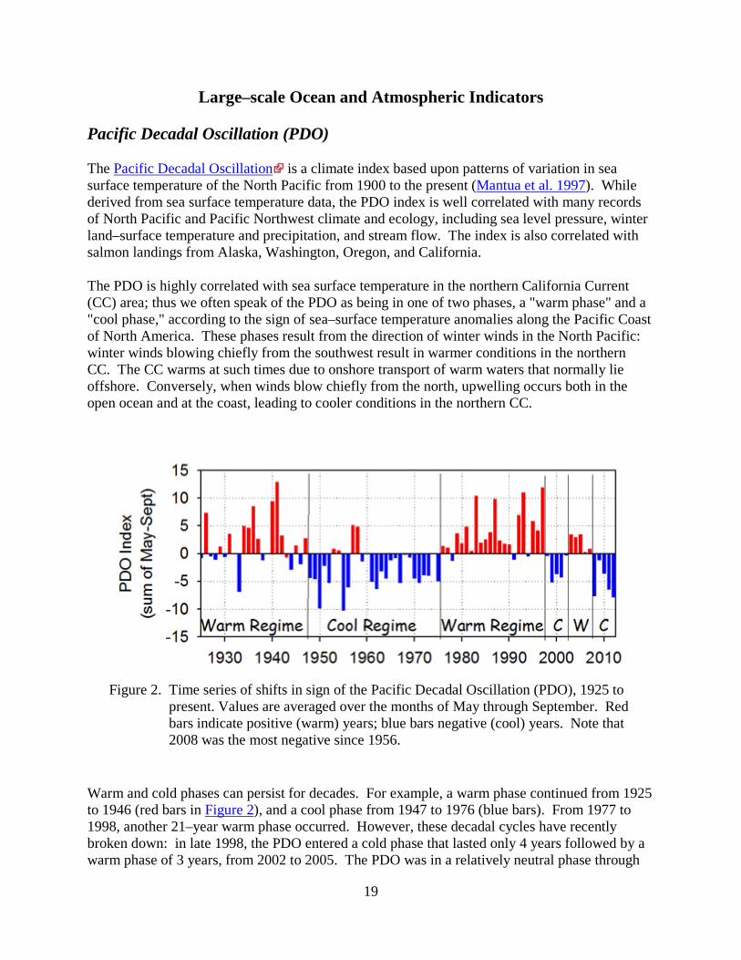
The Pacific Decadal Oscillation is a climate index based upon patterns of variation in sea surface temperature of the North Pacific from 1900 to the present (Mantua et al. 1997). While derived from sea surface temperature data, the PDO index is well correlated with many records of North Pacific and Pacific Northwest climate and ecology, including sea level pressure, winter land–surface temperature and precipitation, and stream flow. The index is also correlated with salmon landings from Alaska, Washington, Oregon, and California.

The PDO is highly correlated with sea surface temperature in the northern California Current (CC) area; thus we often speak of the PDO as being in one of two phases, a "warm phase" and a "cool phase," according to the sign of sea–surface temperature anomalies along the Pacific Coast of North America. These phases result from the direction of winter winds in the North Pacific: winter winds blowing chiefly from the southwest result in warmer conditions in the northern CC. The CC warms at such times due to onshore transport of warm waters that normally lie offshore. Conversely, when winds blow chiefly from the north, upwelling occurs both in the open ocean and at the coast, leading to cooler conditions in the northern CC.

Figure 2. Time series of shifts in sign of the Pacific Decadal Oscillation (PDO), 1925 to present. Values are averaged over the months of May through September. Red bars indicate positive (warm) years; blue bars negative (cool) years. Note that 2008 was the most negative since 1956.

Warm and cold phases can persist for decades. For example, a warm phase continued from 1925 to 1946 (red bars in Figure 2), and a cool phase from 1947 to 1976 (blue bars). From 1977 to 1998, another 21–year warm phase occurred. However, these decadal cycles have recently broken down: in late 1998, the PDO entered a cold phase that lasted only 4 years followed by a warm phase of 3 years, from 2002 to 2005. The PDO was in a relatively neutral phase through

20

August 2007, but abruptly changed in September 2007 to a negative phase that lasted nearly 2 years, through July 2009. The PDO then reverted to a positive phase in August 2009 (Figure 5) because of a moderate El Niño event that developed at the equator during fall/winter 2009–2010. This positive signal continued for 10 months (August 2009–May 2010) until June 2010, when persistently negative values of the PDO initiated and have remained strongly negative through autumn 2012.

Dr. Nathan Mantua and his colleagues were the first to show that adult salmon catches in the Northeast Pacific were correlated with the Pacific Decadal Oscillation (Mantua et al. 1997). They noted that in the Pacific Northwest, the cool PDO years of 1947–1976 coincided with high returns of Chinook and coho salmon to Oregon rivers. Conversely, during the warm PDO cycle that followed (1977–1998), salmon numbers declined steadily.

21

Figure 3. Upper panel shows summer average PDO, 1965–present; middle panel shows anomalies in counts of adult spring Chinook passing Bonneville Dam for the same period; lower panel shows survival of hatchery coho salmon from 1965–present. Vertical lines indicate climate–shift points in 1977 and 1998.

The listing of several salmon stocks as threatened or endangered under the U.S. Endangered Species Act coincides with a prolonged period of poor ocean conditions that began in the early 1990s. This is illustrated in Figure 3, which shows average PDO values in summer vs. anomalies in counts of adult spring Chinook at Bonneville Dam. Also shown are percentages of

22

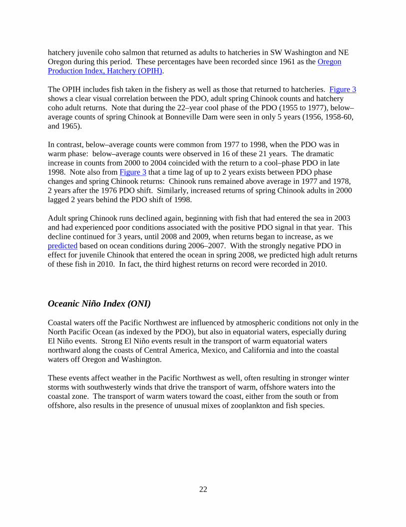
hatchery juvenile coho salmon that returned as adults to hatcheries in SW Washington and NE Oregon during this period. These percentages have been recorded since 1961 as the Oregon Production Index, Hatchery (OPIH).

The OPIH includes fish taken in the fishery as well as those that returned to hatcheries. Figure 3 shows a clear visual correlation between the PDO, adult spring Chinook counts and hatchery coho adult returns. Note that during the 22–year cool phase of the PDO (1955 to 1977), below–average counts of spring Chinook at Bonneville Dam were seen in only 5 years (1956, 1958-60, and 1965).

In contrast, below–average counts were common from 1977 to 1998, when the PDO was in warm phase: below–average counts were observed in 16 of these 21 years. The dramatic increase in counts from 2000 to 2004 coincided with the return to a cool–phase PDO in late 1998. Note also from Figure 3 that a time lag of up to 2 years exists between PDO phase changes and spring Chinook returns: Chinook runs remained above average in 1977 and 1978, 2 years after the 1976 PDO shift. Similarly, increased returns of spring Chinook adults in 2000 lagged 2 years behind the PDO shift of 1998.

Adult spring Chinook runs declined again, beginning with fish that had entered the sea in 2003 and had experienced poor conditions associated with the positive PDO signal in that year. This decline continued for 3 years, until 2008 and 2009, when returns began to increase, as we predicted based on ocean conditions during 2006–2007. With the strongly negative PDO in effect for juvenile Chinook that entered the ocean in spring 2008, we predicted high adult returns of these fish in 2010. In fact, the third highest returns on record were recorded in 2010.

Oceanic Niño Index (ONI)

Coastal waters off the Pacific Northwest are influenced by atmospheric conditions not only in the North Pacific Ocean (as indexed by the PDO), but also in equatorial waters, especially during El Niño events. Strong El Niño events result in the transport of warm equatorial waters northward along the coasts of Central America, Mexico, and California and into the coastal waters off Oregon and Washington.

These events affect weather in the Pacific Northwest as well, often resulting in stronger winter storms with southwesterly winds that drive the transport of warm, offshore waters into the coastal zone. The transport of warm waters toward the coast, either from the south or from offshore, also results in the presence of unusual mixes of zooplankton and fish species.

23

Figure 4. Values of the ONI, 1955 - present. Red bars indicate warm conditions in the equatorial Pacific, blue bars indicate cool conditions in equatorial waters. Large and prolonged El Niño events are indicated by large, positive values of the index: note the > +2 value associated with the 1972, 1983 and 1998 events. Note cool anomalies (La Niña) during 1999-2002 and 2007-spring 2009. A La Niña event developed in equatorial waters from mid-2010 to June 2011, but transitioned to positive values in 2012.

El Niño events have variable and unpredictable effects on coastal waters off Oregon and Washington. While we do not fully understand how El Niño signals are transmitted northward from the equator, we do know that signals can travel through the ocean via Kelvin waves. Kelvin waves propagate northward along the coast of North America and result in transport of warm waters from south to north.

El Niño signals can also be transmitted through atmospheric teleconnections in that El Niño conditions can strengthen the Aleutian Low, a persistent low–pressure air mass over the Gulf of Alaska. Thus adjustments in the strength and location of low–pressure atmospheric cells at the equator can affect our local weather, resulting in more frequent large storms in winter and possible disruption of upwelling winds in spring and summer.

Since 1955, the presence/absence of conditions resulting from the El Niño Southern Oscillation (ENSO) has been gauged using the Oceanic Niño Index, or ONI. A time series of the ONI is shown in Figure 4. Prior to 1977 (during the cool phase of the PDO), El Niño conditions were observed infrequently (note the predominance of blue bars prior to 1977).

24

During these 22 years, cool conditions were observed in only 98 of 266 months. During this same warm phase of the PDO, both the equatorial and northern North Pacific oceans experienced two very large El Niño events (1983-1984 and 1997-1998). There were also two smaller events in 1986 and 1987 and a prolonged event from 1990 to 1995.

Beginning in September 1998, ONI values turned negative and remained so for nearly 4 years, similar to the trend observed in the PDO. The ONI returned to positive in April 2002 and remained so through September 2005, after which negative values returned. Positive values were seen once again, beginning in spring 2009 and remaining through May 2010. In June 2010, negative values became established and persisted into mid 2011 before becoming near-neutral.

Both the PDO and ONI can be viewed as "leading indicators" of ocean conditions, since after a persistent change in sign of either index, ocean conditions in the California Current soon begin to change. The ONI is a good index of El Niño conditions, and one can find information on the status of both El Niño and La Niña at the Climate Prediction Center and other websites maintained by the NOAA National Weather Service. Following the relatively strong El Niño during the winter of 2009-2010, the northern California Current experienced a rapid switch to La Niña conditions. The switch was reflected in both a drop in sea surface temperatures (Figure 5) and a later decrease in copepod biodiversity (Figure 21).

25

Local and Regional Physical Indicators

Temperature Anomalies

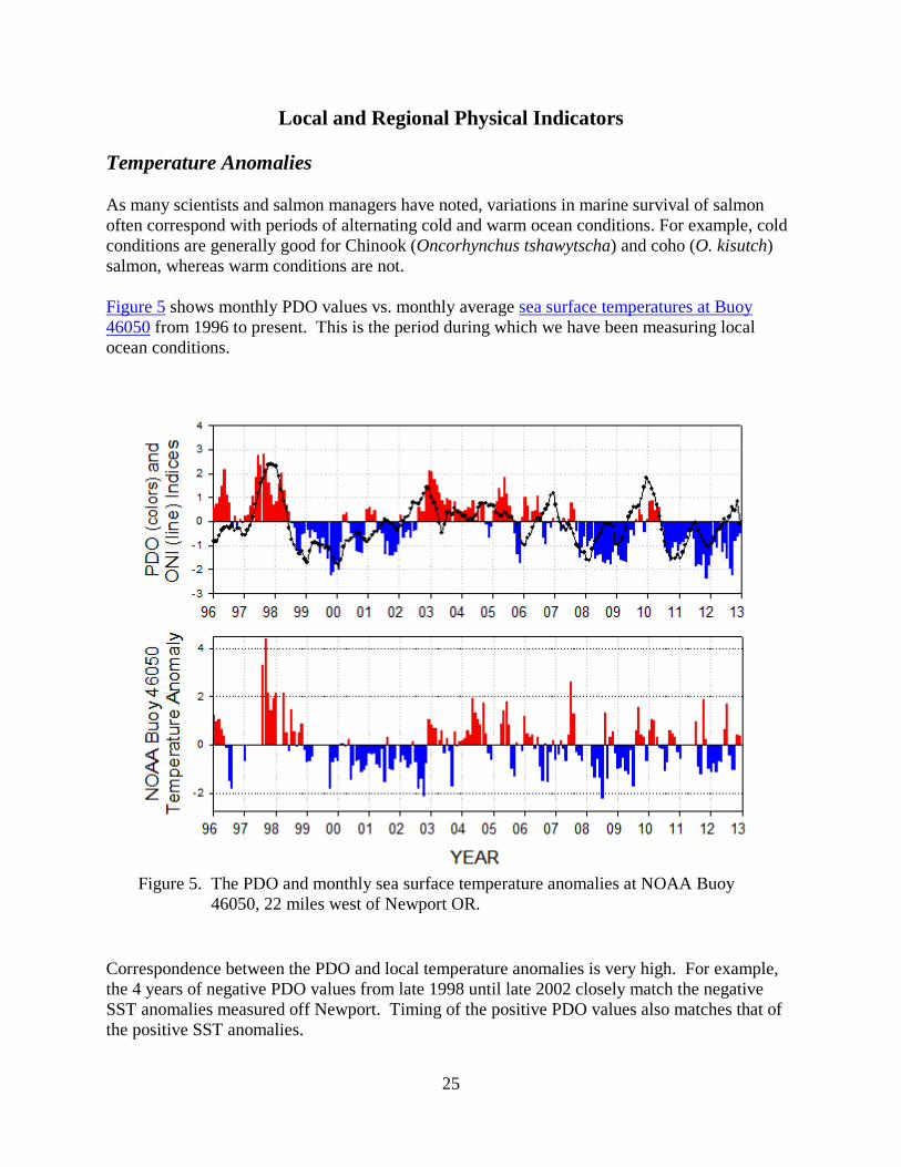
As many scientists and salmon managers have noted, variations in marine survival of salmon often correspond with periods of alternating cold and warm ocean conditions. For example, cold conditions are generally good for Chinook (Oncorhynchus tshawytscha) and coho (O. kisutch) salmon, whereas warm conditions are not.

Figure 5 shows monthly PDO values vs. monthly average sea surface temperatures at Buoy 46050 from 1996 to present. This is the period during which we have been measuring local ocean conditions.

Figure 5. The PDO and monthly sea surface temperature anomalies at NOAA Buoy 46050, 22 miles west of Newport OR.

Correspondence between the PDO and local temperature anomalies is very high. For example, the 4 years of negative PDO values from late 1998 until late 2002 closely match the negative SST anomalies measured off Newport. Timing of the positive PDO values also matches that of the positive SST anomalies.

26

This suggests that changes in basin–scale forcing results in local SST changes, and that local changes may be due to differences in transport of water out of the North Pacific into the northern California Current. The data also verify that we can often use local SST as a proxy for the PDO. However, there are periods in which local and regional changes in the northern CC may diverge from the PDO pattern for short periods (usually less than a few months).

Buoy temperatures clearly identify warm and cold ocean conditions. During the 1997–1998 El Niño event, summer water temperatures were 1–2°C above normal, whereas during 1999–2002, they were 2°C cooler than normal (Figure 5). The summers of 2003–2005 were again warm, and some months showed positive SST anomalies that exceeded even those seen during the 1998 El Niño event. Some marine scientists refer to 2003–2005 as having "El Niño–like" conditions. In contrast, summertime SSTs were cooler than normal during summer 2006 and 2008 and during winters of 2006–2008. Cool temperatures persisted from mid–2007 through mid–2009, with only a few months of warmer–than–average temperatures (autumn 2008 and late summer 2009).

However, in autumn 2009, an El Niño event arrived (as predicted by NOAA scientists) and SSTs warmed, with anomalies of nearly +1°C. These warm temperatures persisted through the first half of 2010. In spring 2010, a La Niña (cooling) event began, and SSTs responded with negative anomalies of –1.5°C through late summer and autumn.

Note also in Figure 5 that there is a time lag between a sign change of the PDO and a change in local SSTs. In 1998, the PDO changed to negative in July, and SSTs cooled in December. In 2002, the opposite pattern was seen, with a PDO signal changing to positive in August followed by warmer SSTs in December. Thus, it takes 5–6 months for a signal in the North Pacific to propagate to coastal waters.

These measurements show that basin–scale indicators such as the PDO do manifest themselves locally: local SSTs change in response to physical shifting on a North Pacific basin scale. Other local ecosystem indicators influenced by the basin–scale indicators (and discussed here) include source waters that feed into the northern California Current, zooplankton and forage fish community types, and abundance of salmon predators such as hake and sea birds.

Thus, local variables respond to change that occurs on a broad spectrum of spatial scales. These range from basin–scale changes, which are indexed chiefly by the PDO, to local and regional changes, such as those related to shifts in the jet stream, atmospheric pressure, and surface wind patterns.

During 2011, the buoy was out of service from Jan 10 - July 5. Initial temperatures in January were cooler than average, reflecting the La Nina conditions.

27

Figure 6. Daily sea surface temperature anomalies measured at NOAA Buoy 46050, located 22 miles off Newport, OR.

Figure 7 summarizes temperature measurements made during our biweekly cruises made off Newport Oregon, at station NH 05. Seasonal averages for winter (Nov-Mar) and summer (May–Sep) show that temperatures in the upper 20 m of the water column were much cooler than average in the beginning of the year and slightly cooler than average during the summer.

28

Figure 7. Upper panel shows the average temperature in the upper 20 m of the water column at Station NH 05 (located 5 miles off Newport, Oregon) since 1996. The lower panels depict the upper 20 m temperature anomalies over the same years during summer (left; May–September) and winter (right; Nov – Mar).

Coastal Upwelling

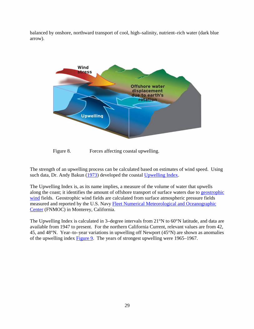
An important process affecting primary productivity during the spring and summer off the Pacific Northwest is coastal upwelling. Upwelling is caused by northerly winds that blow along the Oregon coast from April to September. These winds transport offshore surface water southward (orange arrow in Figure 8), with a component transported away from the coastline (to the right of the wind, light green arrow). This offshore, southward transport of surface waters is

29

balanced by onshore, northward transport of cool, high–salinity, nutrient–rich water (dark blue arrow).

Figure 8. Forces affecting coastal upwelling.

The strength of an upwelling process can be calculated based on estimates of wind speed. Using such data, Dr. Andy Bakun (1973) developed the coastal Upwelling Index.

The Upwelling Index is, as its name implies, a measure of the volume of water that upwells along the coast; it identifies the amount of offshore transport of surface waters due to geostrophic wind fields. Geostrophic wind fields are calculated from surface atmospheric pressure fields measured and reported by the U.S. Navy Fleet Numerical Meteorological and Oceanographic Center (FNMOC) in Monterey, California.

The Upwelling Index is calculated in 3–degree intervals from 21°N to 60°N latitude, and data are available from 1947 to present. For the northern California Current, relevant values are from 42, 45, and 48°N. Year–to–year variations in upwelling off Newport (45°N) are shown as anomalies of the upwelling index Figure 9. The years of strongest upwelling were 1965–1967.

30

Figure 9. Anomalies of the coastal Upwelling Index during May to September each

year, 1946 - present

Upwelling was anomalously weak in all but 8 of the 21 years from summer 1976 to summer 1997, and this is expected during warm PDO phases. When the PDO was in a cool phase (late 1998–2003), upwelling strengthened. With the change in PDO sign to positive in 2004–2005, upwelling again weakened.

Many studies have shown correlations between the amount of coastal upwelling and production of various fisheries. The first to show a predictable relationship between coho survival and upwelling were Gunsolus (1978) and Nickelson (1986).

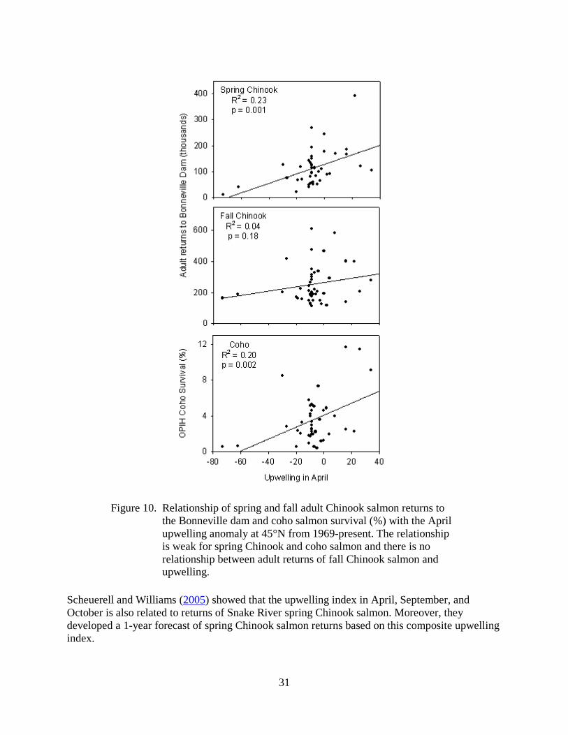
The relationship of spring and fall adult Chinook salmon returns to the Bonneville dam and coho salmon survival (%) with upwelling is shown in Figure 10. The relationship is weak for spring Chinook and coho salmon and there is no relationship with adult returns and upwelling for fall Chinook salmon. Although the relationships are weak, the strongest correlations with survival were found with upwelling in April and upwelling in April and May combined. A significant, but weaker correlation was also found between upwelling and survival during the months of April, May, and June combined.

31

Figure 10. Relationship of spring and fall adult Chinook salmon returns to

the Bonneville dam and coho salmon survival (%) with the April upwelling anomaly at 45°N from 1969-present. The relationship is weak for spring Chinook and coho salmon and there is no relationship between adult returns of fall Chinook salmon and upwelling.

Scheuerell and Williams (2005) showed that the upwelling index in April, September, and October is also related to returns of Snake River spring Chinook salmon. Moreover, they developed a 1-year forecast of spring Chinook salmon returns based on this composite upwelling index.

32

Knowledge of upwelling alone does not always provide good predictions of salmon returns. For example, during the 1998 El Niño event, upwelling was relatively strong, as measured by the upwelling indices; however, plankton production was weak. This occurred because the deep source waters for upwelling were warm and nutrient–poor. Low levels of plankton production may have impacted all trophic levels up the food chain.

Upwelling was also strong during summer 2006, yet SST anomalies only averaged −0.3°C. On the other hand, upwelling was relatively weak during the summers of 2007 and 2008, yet these summers had some of the coldest temperatures in the time series, −1.0°C. These observations demonstrate that some care is required when interpreting a given upwelling index. We hypothesize that although upwelling is necessary to stimulate plankton production, its impact is greatest during negative phases of the PDO.

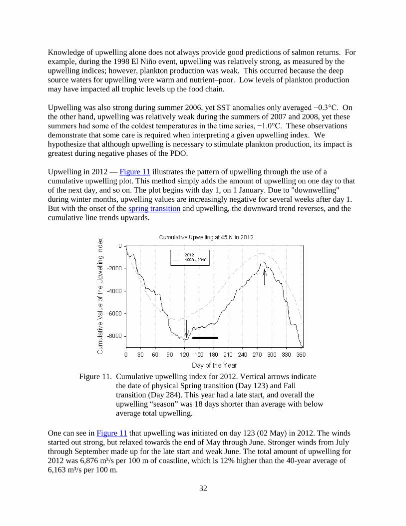
Upwelling in 2012 — Figure 11 illustrates the pattern of upwelling through the use of a cumulative upwelling plot. This method simply adds the amount of upwelling on one day to that of the next day, and so on. The plot begins with day 1, on 1 January. Due to "downwelling" during winter months, upwelling values are increasingly negative for several weeks after day 1. But with the onset of the spring transition and upwelling, the downward trend reverses, and the cumulative line trends upwards.

Figure 11. Cumulative upwelling index for 2012. Vertical arrows indicate the date of physical Spring transition (Day 123) and Fall transition (Day 284). This year had a late start, and overall the upwelling “season” was 18 days shorter than average with below average total upwelling.

One can see in Figure 11 that upwelling was initiated on day 123 (02 May) in 2012. The winds started out strong, but relaxed towards the end of May through June. Stronger winds from July through September made up for the late start and weak June. The total amount of upwelling for 2012 was 6,876 m³/s per 100 m of coastline, which is 12% higher than the 40-year average of 6,163 m³/s per 100 m.

33

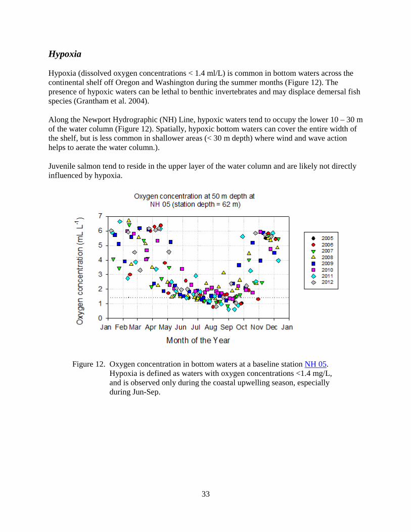
Hypoxia

Hypoxia (dissolved oxygen concentrations < 1.4 ml/L) is common in bottom waters across the continental shelf off Oregon and Washington during the summer months (Figure 12). The presence of hypoxic waters can be lethal to benthic invertebrates and may displace demersal fish species (Grantham et al. 2004).

Along the Newport Hydrographic (NH) Line, hypoxic waters tend to occupy the lower 10 – 30 m of the water column (Figure 12). Spatially, hypoxic bottom waters can cover the entire width of the shelf, but is less common in shallower areas (< 30 m depth) where wind and wave action helps to aerate the water column.).

Juvenile salmon tend to reside in the upper layer of the water column and are likely not directly influenced by hypoxia.

Figure 12. Oxygen concentration in bottom waters at a baseline station NH 05.

Hypoxia is defined as waters with oxygen concentrations <1.4 mg/L, and is observed only during the coastal upwelling season, especially during Jun-Sep.

34

Physical Spring Transition

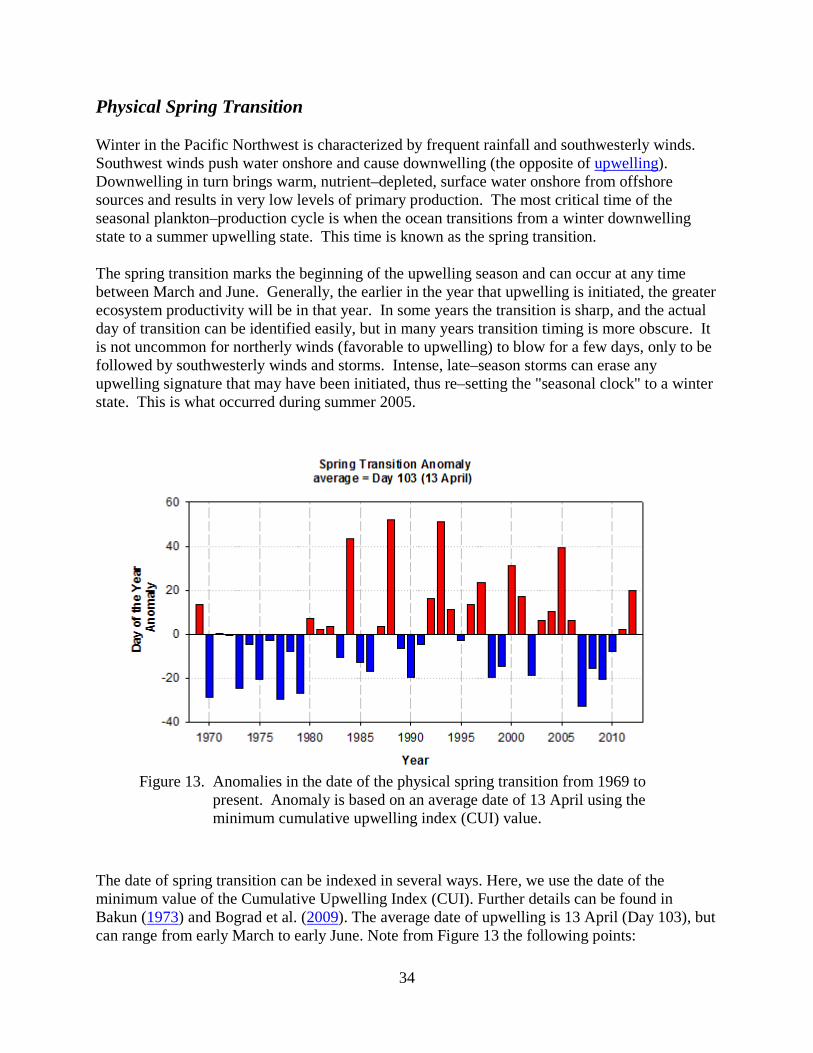
Winter in the Pacific Northwest is characterized by frequent rainfall and southwesterly winds. Southwest winds push water onshore and cause downwelling (the opposite of upwelling). Downwelling in turn brings warm, nutrient–depleted, surface water onshore from offshore sources and results in very low levels of primary production. The most critical time of the seasonal plankton–production cycle is when the ocean transitions from a winter downwelling state to a summer upwelling state. This time is known as the spring transition.

The spring transition marks the beginning of the upwelling season and can occur at any time between March and June. Generally, the earlier in the year that upwelling is initiated, the greater ecosystem productivity will be in that year. In some years the transition is sharp, and the actual day of transition can be identified easily, but in many years transition timing is more obscure. It is not uncommon for northerly winds (favorable to upwelling) to blow for a few days, only to be followed by southwesterly winds and storms. Intense, late–season storms can erase any upwelling signature that may have been initiated, thus re–setting the "seasonal clock" to a winter state. This is what occurred during summer 2005.

Figure 13. Anomalies in the date of the physical spring transition from 1969 to present. Anomaly is based on an average date of 13 April using the minimum cumulative upwelling index (CUI) value.

The date of spring transition can be indexed in several ways. Here, we use the date of the minimum value of the Cumulative Upwelling Index (CUI). Further details can be found in Bakun (1973) and Bograd et al. (2009). The average date of upwelling is 13 April (Day 103), but can range from early March to early June. Note from Figure 13 the following points:

35

• Most spring transition dates during the pre–1977 cool–phase PDO were earlier than average.

• Spring transition dates from the 1980s and 1990s did not reflect changes in either the PDO (Figure 2) or the Multivariate ENSO index (Figure 4).

• The period of early transition dates from 1985 to 1990 correlates well with the high salmon survival in the late 1980s (see Figure 3).

Figure 14. Coho survival vs. day of spring transition. Date of spring transition is based

on the lowest cumulative Upwelling Index value. Data are from 1969 to present.

Figure 14 shows that hatchery adult coho salmon returns are correlated with the spring transition, similar to results found by Logerwell (Logerwell et al. 2003). An analysis using smolt–to–adult return rates of Snake River spring/summer Chinook (from Scheuerell and Williams 2005), or using counts of either spring or fall Chinook at Bonneville Dam (from the DART website), did not reveal any significant correlations.

Other measures of the spring transition include ones from:

• Dr. Mike Kosro, College of Earth, Ocean and Atmospheric Sciences (CEOAS), Oregon State University, who operates an array of coastal radars that are designed to track the speed and direction of currents at the sea surface. He produces daily charts showing ocean surface current vectors, and from those one can clearly see when surface waters are moving south (due to upwelling) or north (due to downwelling). By scanning progressive images, the date of transition can be visualized.

36

• Dr. Steve Pierce and Dr. Jack Barth, CEOAS, Oregon State University, use local wind data from Newport, Oregon and produce annual plots of the start and end to the upwelling season based on the change in alongshore windstress.

• Logerwell et al. (2003) indexed the spring transition date based on the first day when the value of the 10–day running average for upwelling was positive and the value of the 10–day running average for sea level was negative. This index is no longer regularly updated and made available on-line.

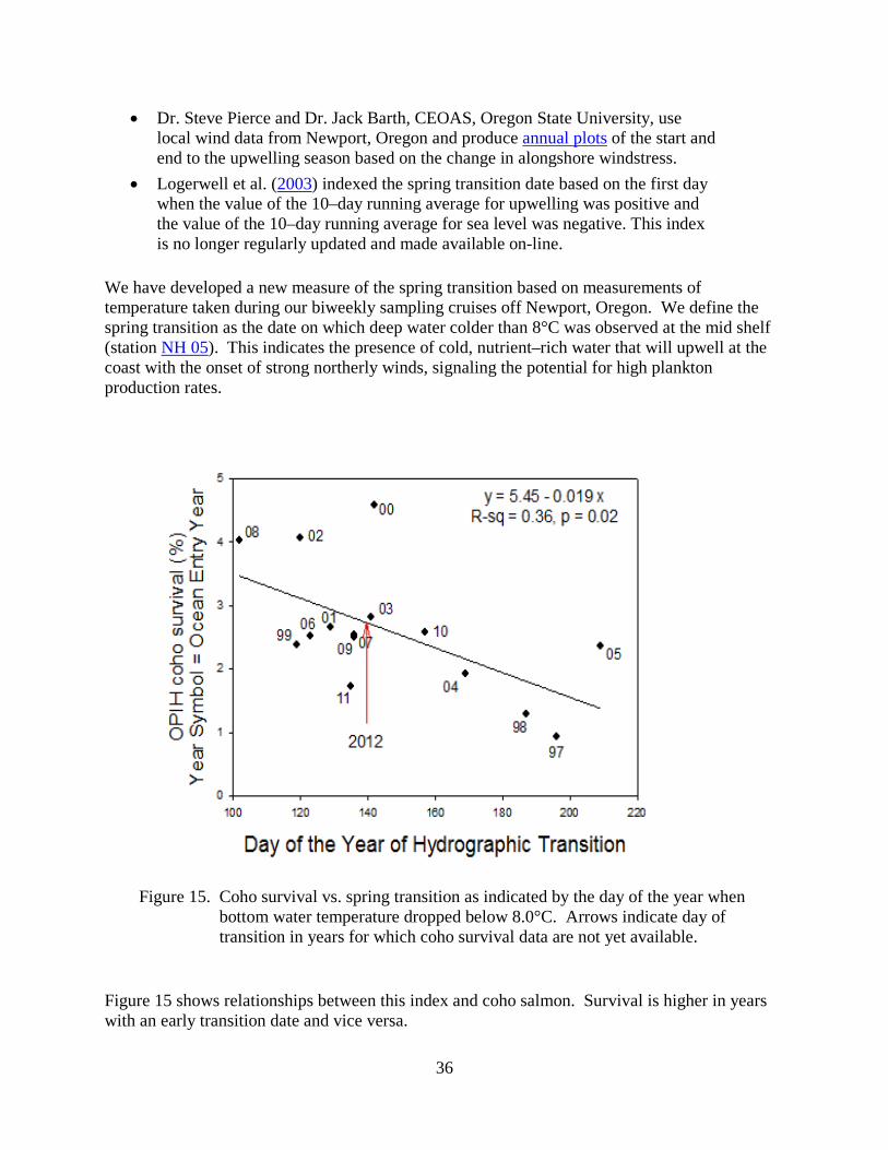
We have developed a new measure of the spring transition based on measurements of temperature taken during our biweekly sampling cruises off Newport, Oregon. We define the spring transition as the date on which deep water colder than 8°C was observed at the mid shelf (station NH 05). This indicates the presence of cold, nutrient–rich water that will upwell at the coast with the onset of strong northerly winds, signaling the potential for high plankton production rates.

Figure 15. Coho survival vs. spring transition as indicated by the day of the year when

bottom water temperature dropped below 8.0°C. Arrows indicate day of transition in years for which coho survival data are not yet available.

Figure 15 shows relationships between this index and coho salmon. Survival is higher in years with an early transition date and vice versa.

37

Deep–Water Temperature and Salinity

Phase changes of the Pacific Decadal Oscillation are associated with alternating changes in wind speed and direction over the North Pacific. Northerly winds result in upwelling (and a negative PDO) and southerly winds, downwelling (and a positive PDO) throughout the Gulf of Alaska and California Current. These winds in turn affect transport of water into the Northern California Current (NCC). Northerly winds transport water from the north whereas southwesterly winds transport water from the west (offshore) and south.

Thus, the phase of the PDO can both express itself and be identified by the presence of different water types in the northern CC. This led us to develop a "water type indicator," the value of which points to the type of water that will upwell at the coast. Again, cold, salty water of subarctic origin is nutrient–rich, whereas the relatively warm and fresh water of the offshore North Pacific Current is nutrient depleted.

Figure 16 shows average salinity and temperature measured at the 50–m depth from station NH 05 (shown in Figure 1). These measurements were taken during biweekly sampling cruises that began in 1997 and continue to the present.

From these data, two patterns have become clear: first, the years 1997-1998 (and to a lesser extent 2003 and 2006) were warmer than average, and corresponded to a warm-phase PDO. Second, the years 1999-2002 and 2007-2012 were colder than average and corresponded to a cool-phase PDO (and to negative SST anomalies at Buoy 46050).

38

Figure 16. Mean salinity (upper panel) and temperature (lower panel) at the 50–m depth at station NH 05 (average water depth 60 m) averaged over all cruises from May to September each year.

Figure 17 shows the same data, but as a scatter diagram, illustrating several noteworthy points. First, during the El Niño event of 1997-1998, deep waters on the continental shelf off Newport were warm and relatively fresh. Second, during the contrasting negative-phase PDO years of 1999-2002 and 2007-2008, these waters were cold and relatively salty or intermediate, as in 2009-2012.

39

Figure 17. Upper panel Scattergram shows average temperature and salinity values during the April–June upwelling season from 1997–present. Middle panel Scattergram of the same average values during May–September 1997–present. Lower panel Average temperature and salinity values during July–September 1997–present.

40

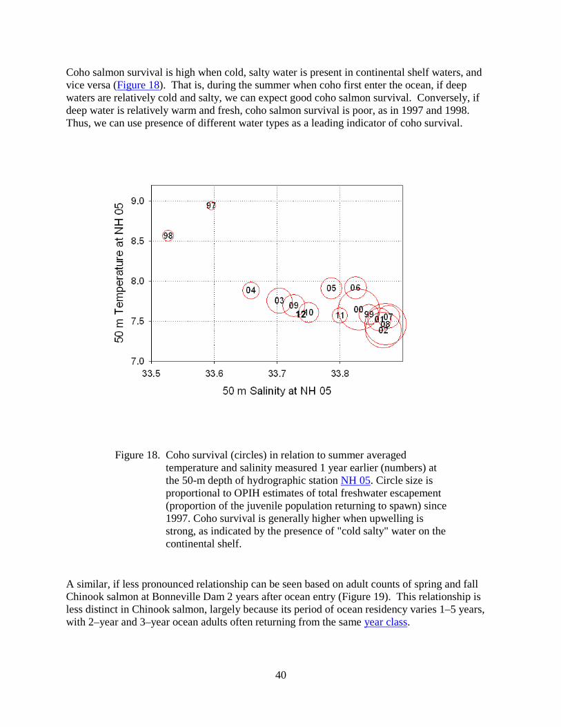
Coho salmon survival is high when cold, salty water is present in continental shelf waters, and vice versa (Figure 18). That is, during the summer when coho first enter the ocean, if deep waters are relatively cold and salty, we can expect good coho salmon survival. Conversely, if deep water is relatively warm and fresh, coho salmon survival is poor, as in 1997 and 1998. Thus, we can use presence of different water types as a leading indicator of coho survival.

Figure 18. Coho survival (circles) in relation to summer averaged temperature and salinity measured 1 year earlier (numbers) at the 50-m depth of hydrographic station NH 05. Circle size is proportional to OPIH estimates of total freshwater escapement (proportion of the juvenile population returning to spawn) since 1997. Coho survival is generally higher when upwelling is strong, as indicated by the presence of "cold salty" water on the continental shelf.

A similar, if less pronounced relationship can be seen based on adult counts of spring and fall Chinook salmon at Bonneville Dam 2 years after ocean entry (Figure 19). This relationship is less distinct in Chinook salmon, largely because its period of ocean residency varies 1–5 years, with 2–year and 3–year ocean adults often returning from the same year class.

41

Figure 19. Percent returns of Chinook salmon to the Bonneville Dam (circles) in relation to summer averaged temperature and salinity measured 2 years earlier (numbers) at the 50-m depth of hydrographic station NH 05. The size of each bubble is proportional to the highest returns since 1997.

Moreover, the Columbia River fall Chinook salmon exhibits two distinct life–history types: the lower–river tule, which returns most frequently as a 2–ocean adult; and the upriver bright, which more often returns as a 3–ocean adult. Coho on the other hand, spends 18 months in the ocean, entering in the spring of one year and returning in the fall of the next.

Despite the variability in age class among Chinook stocks, it is clear that the 1997 El Niño can probably be blamed for low counts of adult Chinook at Bonneville in 1999. High counts of adult Chinook at Bonneville from 2001 to 2003 were accompanied by a 4–year period of very cold and salty ocean conditions. Likewise, the declining returns of 2005–2007 were from fish that entered the ocean in 2003–2005, a period when the PDO was positive, and deep waters were relatively warm and fresh. Finally, the high adult returns in 2010 reflect the highly favorable ocean conditions encountered by juvenile Chinook migrants in 2008.

Local Biological Indicators

Copepod Biodiversity

Being planktonic, copepods drift with the ocean currents; therefore, they are good indicators of the type of water being transported into the Northern California Current. Copepod biodiversity (or species richness) is a simple measure of the number of copepod species in a plankton sample and can be used to index the types of water masses present in the coastal zone off Oregon and Washington.

42

For example, the presence of subtropical species off Oregon indicates transport of subtropical water into the northern California Current from the south. Likewise, the presence of coastal, subarctic species indicates transport of coastal, subarctic waters from the north.

Thus the presence of certain copepod species offers corroborative evidence that the changes in water temperature and salinity observed during our monitoring cruises were in fact measuring different water types. Figure 20 shows average copepod species richness (i.e., the average number of species from all plankton samples) for each month from 1996 to 2004 at station NH 05.

Figure 20. Vertical bars are the climatology of monthly averaged copepod species richness, a measure of biodiversity, at station NH 05 off Newport OR. Dashed line with filled triangles is the climatology of monthly averaged copepod biomass (Y–axis on right side of graph). Note the inverse relationship between copepod biodiversity and copepod biomass.

Generally, species diversity is lower during the summer months and higher during winter months. This pattern is the result of seasonally varying circulation patterns of coastal currents. During summer, source waters to the Oregon coast flow from the north, out of the coastal subarctic Pacific. This is a region of low species diversity.

Conversely, during winter, the source waters originate offshore and from the south, bringing warm, low–salinity water into the coastal waters of the northern California Current. With it comes a more species–rich planktonic fauna with subtropical neritic and warm–water offshore affinities. Variations in species richness from the average values shown in Figure 20 index the relative contribution of subarctic vs. subtropical water to the northern California Current.

43

The annual cycle of copepod biodiversity and copepod biomass are related in an inverse manner (Figure 20). During the winter months, when biodiversity is high, the biomass of copepods is low; during summer, when biodiversity is low, biomass of copepods is high. We also find that during summers when biodiversity is high that copepod biomass is low (not shown).

Figure 21 shows monthly anomalies of copepod species richness during 1996-present. This time series is derived by taking the average number of species for each month, then subtracting the observed monthly average for that month.

Figure 21. Upper panel shows time series of the PDO (bars) and ONI (line) during 1996-present. Lower panel shows anomalies in copepod species richness during the same period. Note the brief lag between long-term persistent shifts in the PDO and ONI and anomalies in copepod species richness, as seen in 1998, 2002, 2007, and 2010.

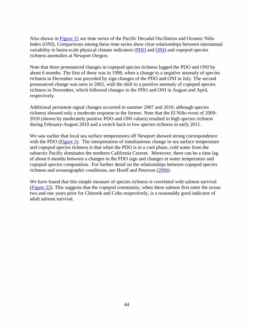
44

Also shown in Figure 21 are time series of the Pacific Decadal Oscillation and Oceanic Niño Index (ONI). Comparisons among these time series show clear relationships between interannual variability in basin-scale physical climate indicators (PDO and ONI) and copepod species richness anomalies at Newport Oregon.

Note that three pronounced changes in copepod species richness lagged the PDO and ONI by about 6 months. The first of these was in 1998, when a change to a negative anomaly of species richness in December was preceded by sign changes of the PDO and ONI in July. The second pronounced change was seen in 2002, with the shift to a positive anomaly of copepod species richness in November, which followed changes in the PDO and ONI in August and April, respectively.

Additional persistent signal changes occurred in summer 2007 and 2010, although species richness showed only a moderate response to the former. Note that the El Niño event of 2009-2010 (shown by moderately positive PDO and ONI values) resulted in high species richness during February-August 2010 and a switch back to low species richness in early 2011.

We saw earlier that local sea surface temperatures off Newport showed strong correspondence with the PDO (Figure 5). The interpretation of simultaneous change in sea surface temperature and copepod species richness is that when the PDO is in a cool phase, cold water from the subarctic Pacific dominates the northern California Current. Moreover, there can be a time lag of about 6 months between a changes in the PDO sign and changes in water temperature and copepod species composition. For further detail on the relationships between copepod species richness and oceanographic conditions, see Hooff and Peterson (2006).

We have found that this simple measure of species richness is correlated with salmon survival (Figure 22). This suggests that the copepod community, when these salmon first enter the ocean two and one years prior for Chinook and Coho respectively, is a reasonably good indicator of adult salmon survival.

45

Figure 22. Relationship of Spring and Fall Chinook adult returns to the

Bonneville Dam, and Coho salmon survival (OPIH) to the copepod species richness anomaly when these fish first enter the ocean 2 and 1 years prior (Chinook and Coho respectively) from 1996 - present.

46

The relationship with salmon survival and copepod species richness is somewhat biased and complicated by the trend towards increasing species richness with time. Figure 23 shows that species richness has increased at a rate of 4.4 species over the past 40 years. Although this increase in biodiversity may be due to climate change, it is probably too soon to draw this conclusion (see Peterson 2009).

Figure 23. Upper panel shows time series of copepod species richness from 1969 to present. Note that the number of copepod species has been increasing over the past decade compared to the 1970s. Red triangles represent winter (Oct - April) and black circles represent summer (May - Sept). Lower panelshows the same time series from 1996 to present to highlight the among-year differences. Red triangles represent winter, black circles summer, and green circles indicate summer-averaged values. This figure illustrates the trend towards increasing copepod biodiversity, especially apparent when comparing the cool years of 1999-2002 to the recent cool years of 2007-2009.

47

Northern and Southern Copepod Anomalies

To explore the relationship between water type, copepod species richness, and the PDO, we developed two indices based on the affinities of copepods for different water types. The dominant copepod species occurring off Oregon at NH 05 were classed into two groups: those with cold–water and those with warm–water affinities. The cold–water (boreal or northern) group included the copepods Pseudocalanus mimus, Acartia longiremis, and Calanus marshallae. The warm–water group included the subtropical or southern species Mesocalanus tenuicornis, Paracalanus parvus, Ctenocalanus vanus, Clausocalanus pergens, Clausocalanus arcuicornis and Clausocalanus parapergens, Calocalanus styliremis, and Corycaeus anglicus.

Figure 24. The Pacific Decadal Oscillation (upper), and northern copepod biomass anomalies (lower), from 1969 to present. Biomass values are log base-10 in units of mg carbon m–3.

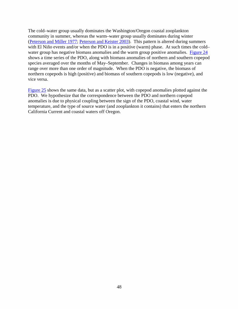
48

The cold–water group usually dominates the Washington/Oregon coastal zooplankton community in summer, whereas the warm–water group usually dominates during winter (Peterson and Miller 1977; Peterson and Keister 2003). This pattern is altered during summers with El Niño events and/or when the PDO is in a positive (warm) phase. At such times the cold–water group has negative biomass anomalies and the warm group positive anomalies. Figure 24 shows a time series of the PDO, along with biomass anomalies of northern and southern copepod species averaged over the months of May–September. Changes in biomass among years can range over more than one order of magnitude. When the PDO is negative, the biomass of northern copepods is high (positive) and biomass of southern copepods is low (negative), and vice versa.

Figure 25 shows the same data, but as a scatter plot, with copepod anomalies plotted against the PDO. We hypothesize that the correspondence between the PDO and northern copepod anomalies is due to physical coupling between the sign of the PDO, coastal wind, water temperature, and the type of source water (and zooplankton it contains) that enters the northern California Current and coastal waters off Oregon.

49

Figure 25. Regression of northern copepod anomalies vs. the PDO. Units of

biomass are mg carbon m³. Strongly negative PDO values lead to high biomass of cold–water copepods and vice versa. The regression line shown was calculated after excluding the outlying data points from 1998 (an El Niño year) and 2005 (an anomalously warm ocean year).

When winds are strong from the north (leading to cool water conditions and a PDO with a negative sign), cold–water copepod species dominate the ecosystem. During summers characterized by weak northerly or easterly winds, (e.g., 1997–1998 and 2004–2005), the PDO is positive, warm–water conditions dominate, and offshore animals move onshore into the coastal zone.

50

Perhaps the most significant aspect of the northern copepod index is that two of the cold–water species, Calanus marshallae and Pseudocalanus mimus, are lipid–rich. Therefore, an index of northern copepod biomass may also index the amount of lipid (wax–esters and fatty acids) transferred up the food chain. These fatty compounds appear to be essential for many pelagic fishes if they are to grow and survive through the winter successfully. Beamish and Mahnken (2001) provide an example of this for coho salmon.

Conversely, the years dominated by warm water, or southern copepod species, can be significant because these species are smaller and have low lipid reserves. This could result in lower fat content in the bodies of small pelagic fish that feed on "fat–free" warm–water copepod species as opposed to cold–water species. Therefore, salmon feeding on pelagic fish, which in turn have fed on warm–water copepod species, may experience a relatively lower probability of surviving the winter.

The "northern copepod index" appears to be a good predictor of the survival of hatchery coho salmon. Figure 26 shows the correlation between adult returns of coho salmon and northern copepod biomass anomalies during the year when these coho entered the ocean (i.e., OPIH coho values in year y + 1 × copepod biomass in year y).

Figure 26. Regression of OPIH coho survival on the northern copepod biomass

anomalies.

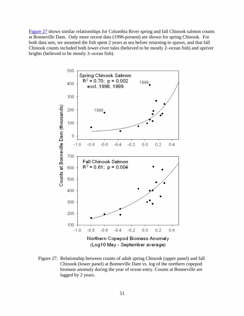
51

Figure 27 shows similar relationships for Columbia River spring and fall Chinook salmon counts at Bonneville Dam. Only more recent data (1996-present) are shown for spring Chinook. For both data sets, we assumed the fish spent 2 years at sea before returning to spawn, and that fall Chinook counts included both lower-river tules (believed to be mostly 2–ocean fish) and upriver brights (believed to be mostly 3–ocean fish).

Figure 27. Relationship between counts of adult spring Chinook (upper panel) and fall

Chinook (lower panel) at Bonneville Dam vs. log of the northern copepod biomass anomaly during the year of ocean entry. Counts at Bonneville are lagged by 2 years.

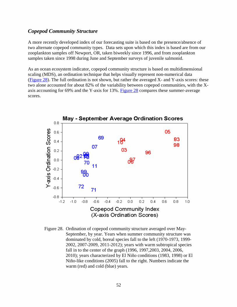
52

Copepod Community Structure

A more recently developed index of our forecasting suite is based on the presence/absence of two alternate copepod community types. Data sets upon which this index is based are from our zooplankton samples off Newport, OR, taken biweekly since 1996, and from zooplankton samples taken since 1998 during June and September surveys of juvenile salmonid.

As an ocean ecosystem indicator, copepod community structure is based on multidimensional scaling (MDS), an ordination technique that helps visually represent non-numerical data (Figure 28). The full ordination is not shown, but rather the averaged X- and Y-axis scores: these two alone accounted for about 82% of the variability between copepod communities, with the X-axis accounting for 69% and the Y-axis for 13%. Figure 28 compares these summer-average scores.

Figure 28. Ordination of copepod community structure averaged over May-

September, by year. Years when summer community structure was dominated by cold, boreal species fall to the left (1970-1973, 1999-2002, 2007-2009, 2011-2012); years with warm subtropical species fall in to the center of the graph (1996, 1997,2003, 2004, 2006, 2010); years characterized by El Niño conditions (1983, 1998) or El Niño-like conditions (2005) fall to the right. Numbers indicate the warm (red) and cold (blue) years.

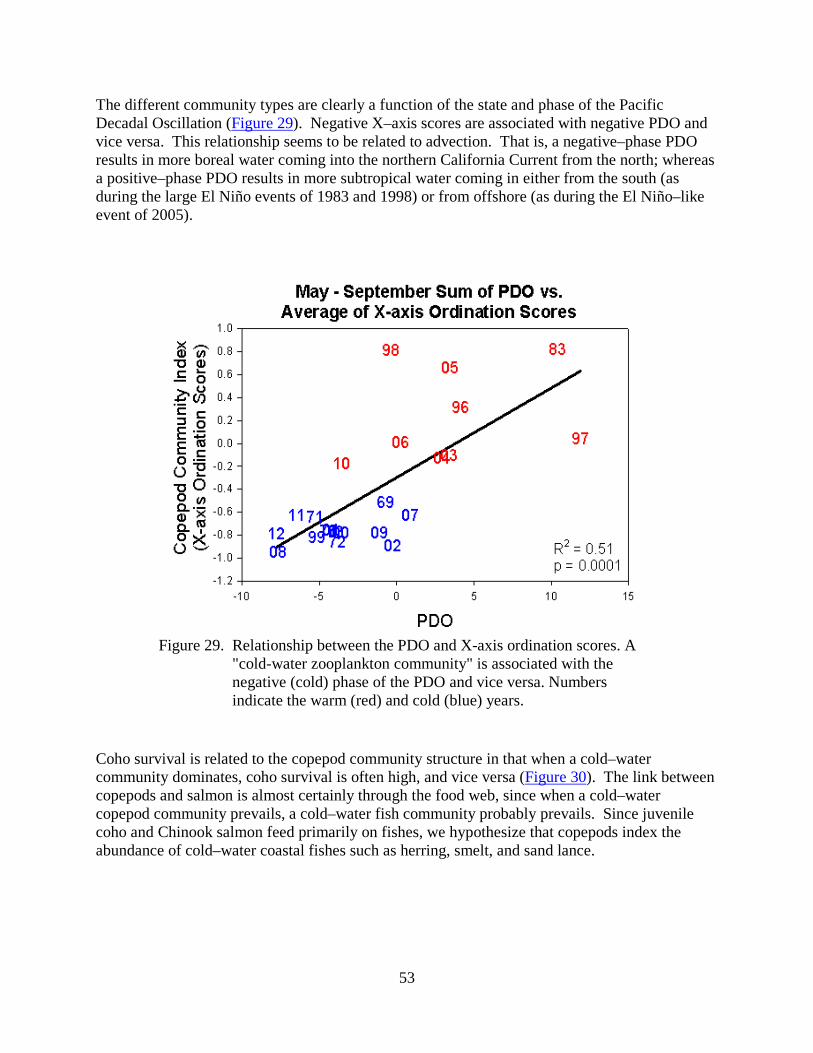
53

The different community types are clearly a function of the state and phase of the Pacific Decadal Oscillation (Figure 29). Negative X–axis scores are associated with negative PDO and vice versa. This relationship seems to be related to advection. That is, a negative–phase PDO results in more boreal water coming into the northern California Current from the north; whereas a positive–phase PDO results in more subtropical water coming in either from the south (as during the large El Niño events of 1983 and 1998) or from offshore (as during the El Niño–like event of 2005).

Figure 29. Relationship between the PDO and X-axis ordination scores. A "cold-water zooplankton community" is associated with the negative (cold) phase of the PDO and vice versa. Numbers indicate the warm (red) and cold (blue) years.

Coho survival is related to the copepod community structure in that when a cold–water community dominates, coho survival is often high, and vice versa (Figure 30). The link between copepods and salmon is almost certainly through the food web, since when a cold–water copepod community prevails, a cold–water fish community probably prevails. Since juvenile coho and Chinook salmon feed primarily on fishes, we hypothesize that copepods index the abundance of cold–water coastal fishes such as herring, smelt, and sand lance.

54

Figure 30. Plot showing the relationship between a) coho smolt-to-adult survival (SAR) (lag 1 year), b) coho adult returns at Bonneville dam (lag 1 year), c) spring Chinook adult returns at Bonneville dam (lag 2 years), and fall Chinook adult returns at Bonneville dam (lag 2 years) versus the copepod community structure index (X-axis ordination score). The stronger the boreal copepod community (negative side of plot), the greater the returns. The X-axis ordination score for May-September 2012 was -0.79, indicating good subsequent salmon survival. Numbers indicate the warm (red) and cold (blue) years.

55

Biological Spring Transition

We suggested earlier that the spring transition could be defined in several ways, one of which was the date that cold water first appeared in mid–shelf waters. In Figure 15, we saw coho survival correlated with the date when cold water first appeared at our baseline station, NH 05. Figure 31 shows a similar relationship, but using the date when a northern (cold–water) copepod community first appeared at station NH 05. We define this as the date of the biological spring transition.

Figure 31. Upper panel: Relationship between coho survival and day of the year when

the copepod community transitioned to a summer community. Lower panel: Relationship between coho survival and length of the biological upwelling season (the number of days that the summer copepod community persisted). Data from the year 1970 were excluded from the regression. Numbers indicate the warm (red) and cold (blue) years.

56

We believe this date may be a more useful indicator of the transition in ocean conditions because it also indicates the first appearance of the kind of food chain that seems most favorable for coho and Chinook salmon; that is, one dominated by large, lipid–rich copepods, euphausiids, and juvenile forage fish.

Thus we suggest that potential feeding conditions for juvenile salmon are more accurately indexed using both northern copepod biomass and the biological spring transition date (as compared to an upwelling index, which is presumed to serve as an index of feeding conditions). We say this in light of the following two instances wherein the upwelling index alone failed to correctly indicate feeding conditions.

First, during El Niño years, or years with extended periods of weak El Niño–like conditions, upwelling can still be strong (as in 1998), but can produce a warm, low–salinity, low–nutrient water type (rather than the expected cold, salty, and nutrient–rich water). Upwelling of this water type results in poor plankton production.

A second example of upwelling as a misleading indicator occurred during 2005, when mean total upwelling levels from May to September were "average." However, the zooplankton community did not transition to a cold–water community until August (Table 6). Therefore, in spite of early upwelling, conditions for salmon feeding, growth, and survival were unfavorable throughout spring and most of summer 2005.

The end of the upwelling season marks the return of a winter community for zooplankton, the timing by which the fall transition is measured.

57

Table 6. Historical dates of the biological spring transition, as measured by the

timing of change in the zooplankton from a winter to a summer community.

Arrival of cold–water copepod community Length of cold–water copepod

presence Year Start date End date (in days) 1970 ~20 Mar 20 Oct 214 1971 20 Mar 6 Nov 231 1983 21 Jul 19 Aug 29 1996 3 Jul 31 Oct 120 1997 15 May 28 Aug 105 1998 20 Sep 24 Sep 4 1999 14 May 4 Nov 174 2000 6 Apr 23 Oct 200 2001 20 Mar 7 Nov 232 2002 18 Apr 1 Nov 197 2003 5 June 3 Oct 120 2004 11 May 14 Oct 156 2005 26 Aug 28 Sep 33 2006 13 Jun 31 Oct 140 2007 22 Mar 31 Dec 284 2008 4 Mar 27 Oct 237 2009 6 Mar 1 Dec 270 2010 18 Jun 24 Nov 159 2011 23 Mar 29 Sep 190 2012 4 May 25 Oct 174

These changes in community type occur because of coastal currents, which reverse in spring to flow from the north with the onset of upwelling. Another reversal occurs in the fall, when the northward–flowing Davidson Current appears on the shelf due to winter downwelling.

Arrival of the “northern” species in spring signals that the ecosystem is primed to begin a productive upwelling season. Also listed is length of the upwelling season in days, as reckoned by the zooplankton. Note that over the years of 2007–2009 and again in 2011, the transition date came very early, in March, whereas in 2012 it came in early May.

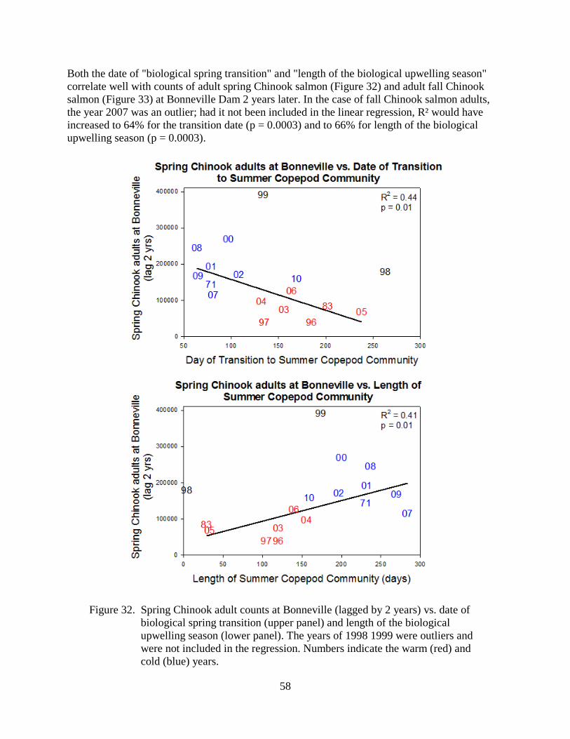
58

Both the date of "biological spring transition" and "length of the biological upwelling season" correlate well with counts of adult spring Chinook salmon (Figure 32) and adult fall Chinook salmon (Figure 33) at Bonneville Dam 2 years later. In the case of fall Chinook salmon adults, the year 2007 was an outlier; had it not been included in the linear regression, R² would have increased to 64% for the transition date (p = 0.0003) and to 66% for length of the biological upwelling season (p = 0.0003).

Figure 32. Spring Chinook adult counts at Bonneville (lagged by 2 years) vs. date of

biological spring transition (upper panel) and length of the biological upwelling season (lower panel). The years of 1998 1999 were outliers and were not included in the regression. Numbers indicate the warm (red) and cold (blue) years.

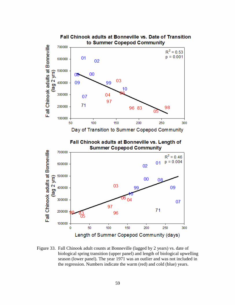
59

Figure 33. Fall Chinook adult counts at Bonneville (lagged by 2 years) vs. date of

biological spring transition (upper panel) and length of biological upwelling season (lower panel). The year 1971 was an outlier and was not included in the regression. Numbers indicate the warm (red) and cold (blue) years.

60

Winter Ichthyoplankton

Marine diets of juvenile coho and Chinook salmon are primarily made up of zero–age winter–spawning juvenile fish such as rockfish, Pacific sand lance, cottids, and smelts (Brodeur et al. 2007; Daly et al. 2009; Table 7). Measures of winter ichthyoplankton biomass are a recent addition to our toolbox. Annual abundance estimates of key salmon prey in winter and early spring provide an indicator of survival in the months before juvenile salmon enter the sea because these estimates reflect the feeding conditions they will potentially encounter. Figure 34 shows the proportions of winter ichthyoplankton biomass composed of food items for juvenile salmon.

Figure 34. Estimates of total winter ichthyoplankton biomass from 1998 to present. Proportions composed of fish larvae considered prey items for juvenile salmon are represented by blue bars.

Winter ichthyoplankton biomass was highest in 2000, 2001, 2008 and 2010 and lowest in 1998, an El Niño year (Figure 34). Years with the highest biomass of the ichthyoplankton typically eaten by juvenile salmon were 2008 and 2000; those with low biomass were 1998 and 2003–2007. The proportion of total ichthyoplankton biomass considered common salmon prey fluctuated from a low of 13.9% in 2006 to a high of 95.0% in 2000. Even though the total biomass of ichthyoplankton was high in 2001, only 18.6% was prey commonly seen in salmon diets.

61

We compared these annual values (log of mean of Jan–March samples) to juvenile coho salmon smolt–to–adult return ratios (SARs), and to counts of adult spring, summer, and fall Chinook salmon at Bonneville Dam to determine whether our index of prey availability is a good predictor of salmon returns. Results of this comparison are shown in Figure 35.

While the abundance of larval fish was low in 2012, the average size of the salmon prey was longer than most years. The overall biomass of winter larvae ranked 6th out of 15 years. Additionally, unlike 2011 when only 7.4% of the total larvae community was considered common salmon prey, 2012 salmon prey comprised 61.9% of the total larval community which is above average (38.8%). The community of salmon prey biomass was dominated by Pacific sand lance (Ammodytes hexapterus) and low in Rockfish (Sebastes spp.) which signifies a cold ocean community and groups with our better ocean survival years. Overall, these patterns suggest moderately good food conditions for salmon in 2012.

62

Coho

OPI

H C

oho

Surv

ival

(%)

1.0

2.0

3.0

4.0

5.0

98

99

00

01

02

03

04050607

08

0910

11

Fall Chinook

Winter Ichthyoplankton Biomass of Salmon Prey (Log mg C 1000m-3)

0.0 0.2 0.4 0.6 0.8 1.0 1.2 1.4 1.6 1.8 2.0100

200

300

400

500

600

700

98

99

00

0102

03

04

05

0607

0809

10

Spring Chinook

Adul

t cou

nts

at B

onne

ville

(tho

usan

ds; l

ag 2

yea

rs)

100

200

300

400

98

00

0102

0304

05

0607

08

09 10

99

Figure 35. Coho salmon smolt-to-adult survival was positively related to winter

ichthyoplankton salmon prey biomass (top panel). The relationship between counts of spring (middle panel) and fall (bottom panel) Chinook adult salmon (lagged by 2 years) at Bonneville Dam and log of the winter ichthyoplankton salmon prey biomass also exhibited a positive relationship.

63

Coho salmon smolt–to–adult survival was positively related to winter ichthyoplankton salmon prey biomass (Figure 35A). The relationship between counts of spring Chinook adult salmon (lagged by 2 years) at Bonneville Dam and log of the winter ichthyoplankton salmon prey biomass exhibited a weak, yet positive relationship (Figure 35B). If the year 1999 is excluded, the relationship is stronger. Counts of fall Chinook salmon adult returns (lagged by 2 years) at Bonneville Dam vs. log of the biomass for winter ichthyoplankton salmon prey exhibited a significant positive relationship (Figure 35C).

Data for these analyses were collected during our sampling cruises along the Newport hydrographic line. Winter ichthyoplankton data shown here were from samples taken 1 January to 31 March. All fish larvae were identified and lengths were measured on a subset of each species per sampling station. Length–to–biomass conversions were made using published values, and total biomass in mg carbon per 1000 m³ at each station was calculated for all sampled larval fish and a subset of fish biomass that included only fish prey typically eaten by juvenile salmon. Table 7 lists common prey eaten by juvenile salmon in their first marine summer and provides data on the size and availability of each.

Table 7. Common prey eaten by juvenile salmon during their first marine summer and their peak spawning season, hatch time and size, estimated days to reach the juvenile stage and average size of prey when eaten by juvenile salmon.

Emmett Hart 1973 Emmett Emmett Hart 1973; Loveet al. 1991 et al. 1991 et al. 1991 CDFG 2009 et al. 2002;

Matareseet al. 19891 winter peak

Source

Ammodytes hexapterus

Engraulis mordax

Pacific sand lance

Pacific herring Northern anchovy

Mean size when eaten by salmonids (mm) 42 34 22 60 39 34

Juvenile size (mm) 30 25–40 15–20 25 20 25–30

Time to juvenile stage (d) 90–120 d 60 d 60 d 70 d 90 d 120–150 d

Size at hatching (mm) 5 7.5 4–5 2–3 3–6 3–6

Jan–MayTime to hatching (d) 21 14 9–14 2–4 10–40 N/A

Nov–Mar Feb–Apr Jan–Feb Feb–Jun Year–round¹

Common name

Sculpin Smelt RockfishSpawning season

Common prey of juvenile salmonidsScientific name

Clupeidae Cottidae Osmeridae Sebastes

64

Catches of Yearling Chinook in June and Coho in September

Numbers of juvenile salmon caught during our June and September trawl surveys can serve as an index or surrogate measure of ocean survival for spring Chinook and coho salmon. Figure 36 shows catch per unit effort (CPUE) during our trawl surveys from 1998 to present.

Figure 36. Average catches of juvenile coho (black bars) and yearling Chinook (red bars) during trawl surveys off the coast of Washington and Oregon. Surveys were conducted in June (upper panel) and September (lower panel) from 1998 to present. Note the difference in the scale of the y-axis between plots.

Catch rates in June were lowest for both species during 2005, but rebounded gradually from 2006-2008, only to decline again. Catches in June 2012 were ranked 2nd out of 15 for yearling Chinook salmon, but only 13th out of the 15 years for yearling coho salmon. September catches of both yearling Chinook and coho salmon were relatively low, ranking 13th and 9th out of the 15 years, respectively.

65

Figure 37 shows the relationship between catches of juvenile Chinook and coho and returns the following year of coho adults and Chinook jacks. In the upper panel, trawl catches of coho in September of year i are correlated with adult counts from the Oregon Production Index of hatchery coho adult returns (OPIH in year i + 1). Similarly, catches of yearling Chinook in June of year i are correlated with counts of spring Chinook jacks at Bonneville Dam in year i + 1.

Figure 37. Regression of the OPIH smolt-to-adult survival (SAR) of coho salmon vs. the average CPUE of juvenile coho salmon catches in trawl surveys the previous September (upper panel). Year represent catches of juvenile fish. The purple open circles indicate observed juvenile CPUE in September 2011 (0.30) and the predicted SAR from both jack returns (1.7%) and from our September 2011 catch (2.8%). The black open circle indicates observed juvenile CPUE (0.13) in September 2012 and predicted SAR (2.5%). 1999 (circled) was excluded from the regression. Regression of spring Chinook salmon jack counts at Bonneville Dam vs. average CPUE of yearling Chinook salmon caught during each June cruise (lower panel). Open black circle indicates observed CPUE in June 2012 (1.32) and the predicted jack returns (28,271). 2010 (circled) was excluded from the regression.

66

Indicators Under Development

Forage Fish and Pacific Hake Abundance

We are developing an index that describes food–web interactions between juvenile salmon and their fish predators, chiefly Pacific whiting, aka Pacific hake. The index is based on interactions between forage fish (e.g., anchovies, smelt and herrings), juvenile salmon, and hake.

This interaction is somewhat complex and probably non–linear: we hypothesize that during warm–ocean years, hake move to continental shelf waters, where salmon are more susceptible to predation. During cold–ocean years, hake feed in deeper waters offshore, near the shelf break, and are not actively feeding in the shallow continental–shelf waters inhabited by juvenile salmon.

During cold ocean conditions, when zooplankton production is high, small forage–fish biomass increases. This increase in forage–fish abundance allows predators to "see" and prey upon forage fish more often than salmon. Most forage fish populations (smelt, herring, and anchovy) do well during cold conditions but tend to crash during warm conditions, but there is a lag of at least 1 year between boom and bust periods. Thus, the interaction among zooplankton production, forage fish abundance, juvenile salmon survival, and hake predation is likely to be non–linear.

We have not analyzed or modeled these interactions. Nevertheless, Figures 38 and 39 demonstrate the pronounced interannual differences in abundance of forage fishes; these are in part related to the cycles gauged by the current ocean ecosystem indicators.

Due to funding constraints, we were unable to conduct any forage fish/predator study cruises in 2012. We believe that this is a promising indicator and hope to resume sampling in the near future.

67

Figure 38. Catches of potential piscivores that prey on juvenile salmon. Pacific hake numbers are usually very high during "warm years" such as the 1998 El Niño event and during the first 2 years of a warm-phase PDO (2003-2004). However, numbers were surprisingly low from 2008-present, despite the 2009 El Niño. Data shown are from the surveys of R. Emmett, conducted May-August 1998-present.

In 2011, Pacific hake, (Figure 38) continued to be found in very low abundances compared to 1998, 2003, and 2004. Low densities were observed during the cool, negative-PDO phases of 1999-2002 and 2008-2011. Conversely, high abundances occurred during the warm, positive-PDO years of 1998, 2003, and 2004. Probably not coincidentally, these years correspond respectively to "good" and "poor" periods for coho survival. We expected high abundance levels for hake in 2005 and 2006 (warm years), but this expectation was not met, due possibly to the timing of their northward migration. That is, hake may have moved further north (off Canada) during the warm years of 2004 and 2005, and thus would have been preying on salmon earlier (May) rather than later (Jun-Jul) in the season.

Forage fish clearly show a 1-year lag between change in ocean phases and population response: anomalously low abundances were observed during the first year of a "cool phase" (1999), and anomalously high abundances were observed during the first year of "warm phase" (2003). This lag time reflects the time it takes for 0-age fish to grow large enough (i.e., 1-year-old) to be captured by the surface trawl. The failure of hake to maintain high abundances in 2005 and 2006, and the 1-year lag in response of forage fish to changes in ocean conditions, contributes to the lack of a linear relationship between salmon catches or survival and forage fish or hake densities. The relationship between salmon marine survival and other fishes appears to be very complicated and probably influenced by additional factors.

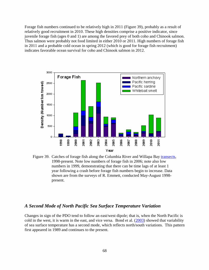
68

Forage fish numbers continued to be relatively high in 2011 (Figure 39), probably as a result of relatively good recruitment in 2010. These high densities comprise a positive indicator, since juvenile forage fish (ages 0 and 1) are among the favored prey of both coho and Chinook salmon. Thus salmon were probably not food limited in either 2010 or 2011. High numbers of forage fish in 2011 and a probable cold ocean in spring 2012 (which is good for forage fish recruitment) indicates favorable ocean survival for coho and Chinook salmon in 2012.

Figure 39. Catches of forage fish along the Columbia River and Willapa Bay transects, 1998-present. Note low numbers of forage fish in 2006; note also low numbers in 1999, demonstrating that there can be time lags of at least 1 year following a crash before forage fish numbers begin to increase. Data shown are from the surveys of R. Emmett, conducted May-August 1998-present.

A Second Mode of North Pacific Sea Surface Temperature Variation

Changes in sign of the PDO tend to follow an east/west dipole; that is, when the North Pacific is cold in the west, it is warm in the east, and vice versa. Bond et al. (2003) showed that variability of sea surface temperature has a second mode, which reflects north/south variations. This pattern first appeared in 1989 and continues to the present.

69

We have not yet investigated this pattern fully because the negative phase of the first mode (the PDO) indicates favorable conditions in the northern California Current, as does the negative phase of the second mode (called the "Victoria" mode). However, oscillation in the second mode would index good vs. poor ecological conditions between the Gulf of Alaska and northern California. Therefore, it is possible that this second mode may serve as a better index of conditions for spring Chinook salmon: conventional wisdom is that spring Chinook resides in the Gulf of Alaska during most of its years at sea.

Phytoplankton Biomass

Based on samples collected along the Newport Hydrographic Line, we developed time series of both total chlorophyll and the fraction of chlorophyll smaller than 10 µm. These data serve as estimates of phytoplankton biomass, and both data types will be used to describe interannual variation in timing of the spring bloom (which can occur between February and April), as well as blooms in summer during July–August upwelling. These measures should provide an index of potential conditions (good vs. poor) for spawning of copepods and euphausiids.

Euphausiid Egg Concentration and Adult Biomass

Euphausiids are a key prey item for juvenile coho and Chinook salmon. Sampling along the Newport Hydrographic Line has also yielded a time series of euphausiid egg abundance. These data may serve as an adult euphausiid biomass index, which should prove useful in comparisons of interannual variation in abundance, survival, and growth for these salmon species.

Since 2000, we have also been sampling at night along the Newport Line in order to capture adult euphausiids. The long–term goal of this sampling is to produce an index of euphausiid biomass in the northern California Current. We are also measuring rates of molting and egg production in living animals in anticipation that these data can be used to calculate euphausiid production.

Interannual Variations in Habitat Area

From the salmon trawl surveys conducted in June and September, we are developing "Habitat Suitability Indices." We hope these will prove useful in providing more precise predictors of the potential success or failure for a given year–class of juvenile salmonids. For example, we have determined that chlorophyll and copepod biomass levels are the best predictors of habitat size for juvenile Chinook salmon. Interannual variation in potential habitat area may also serve as a correlate for salmon survival during the first summer at sea.

70

Salmon Predation Index

A salmon predation index will integrate four variables found to influence predation rates of Columbia River salmon in the ocean (Emmett 2006). These variables are based on the following spring (May/June) measurements:

1. Abundance of Pacific whiting (hake) off the Columbia River 2. Abundance of forage fish off the Columbia River

3. Turbidity of the Columbia River 4. Columbia River flows

Predator and forage–fish abundances are estimated annually from the Predator/Forage Fish Survey, and turbidity will be estimated using satellite imagery, Secchi disc readings, and transmissometer measurements, each of which has been collected since 1998. Initial analyses indicates that during years when hake abundance is low and forage fish abundance, turbidity, and Columbia River flows are high, salmon marine survival is high. However, if even one variable has an opposite value, salmon marine survival declines.

Potential Indices for Future Development

Remaining indices are in very early stages of development or have not yet begun to be developed. These include:

1. An index of Columbia River flow 2. Predictors of coho and spring Chinook jack returns 3. Indices based on salmon feeding and growth 4. Indices based on salmon health (diseases and parasites) 5. Indices that estimate zooplankton production rates, such as

• Euphausiid growth rates from direct measurement of molting rates • Euphausiid growth rates from cohort developmental rates • Copepod growth rates from direct measurement of Calanus egg production rates • Copepod growth rates from empirical growth equations

71

Ocean Sampling Methods

Hydrography, Zooplankton, and Ichthyoplankton

Much of the oceanographic data shown in this report came from sampling along the Newport Hydrographic Line (Figure 40). We sample the coastal waters off Newport at biweekly intervals during the upwelling season in spring, summer, and fall. Sampling cruises are conducted monthly during stormy winter months. This program began in May 1996, but we also have data from these same stations from sampling conducted in 1973 (Peterson and Miller 1975), 1983 (Miller et al. 1985), and summer 1990-1992 (Fessenden 1995).

Figure 40. Transects and stations sampled during cruises by the NOAA Fisheries

Service.

72

Cruises during May 1996-September 2001 were made only during daylight hours because our research vessel, the RV Sacajawea was only 37 ft in length, rendering it unsafe to work at night. With the acquisition of a new and larger research vessel (RV Elakha; 54-ft.) in September 2000, we were able to sample at night. Thus in fall 2000, we began collecting data for an adult euphausiid time series.

This work included measurements of copepod and euphausiid egg production and molting rates. We are also developing a long time–series of copepod and euphausiid production, which should prove useful in evaluating if in fact there are measurable differences in zooplankton production in association with changes in sign of the Pacific Decadal Oscillation.

From 1998 to 2003, we sampled a group of transects from Newport, Oregon down to Crescent City, California five times per year as part of the U.S. Global Ocean Ecosystem Dynamics (GLOBEC) program. Since the GLOBEC project ended, we have continued to sample these same transect lines as frequently as possible. Thus far, we have been able to sample this region in 2004, 2006 and 2008-present, and have extended the Newport Line out to 200 miles from shore. Additionally, we also sample north of the Newport Line at least 3 times per year as part of the Juvenile Salmon sampling program. As a result, the Newport biweekly data are nested within larger scale semi-annual to quarterly surveys, an approach that is useful in helping us interpret locally derived data from the inner portions of the Newport Line.;

At each station, a CTD profile (Conductivity, Temperature, and Depth; Seabird‡ SBE 19 CTD) is taken, and transparency of surface waters is measured (Secchi disc). A bucket of seawater is collected from the surface for analysis of chlorophyll-a and nutrients. A vertical plankton net fitted with a flowmeter is towed from near the sea floor to the surface (or from 100 m to the surface in deeper waters). The plankton net is 0.5 m in diameter with a mesh size of 202 µm. A double oblique tow is made for ichthyoplankton (0.6-m diameter bongo net with 333-µm mesh) over the upper 20 m. Since 2005, CTD casts have included fluorometry (WetLabs fluorometer) and oxygen (Seabird oxygen sensor).

Nutrients are analyzed using a Technicon Autoanalyzer. Chlorophyll–a is extracted from glass–fiber filters in 90% acetone then analyzed using a Turner Designs Fluorometer. Zooplankton samples are processed in the laboratory by subsampling with a Stempel pipette. Species and developmental stage of copepods are enumerated with the aid of a dissecting microscope. Counts are converted to number of individuals per m³ of water using appropriate conversion factors. Biomass is estimated by multiplying the number of individuals per m³ by the dry weight of the taxa (using values from either literature or our own measurements). Carbon content is calculated assuming carbon is 40% of dry weight.

‡ Reference to trade names does not imply endorsement by the National Marine Fisheries Service, NOAA.

73

Juvenile Salmon Sampling Program

Methods

We have sampled juvenile salmon each June and September since 1998 at offshore stations ranging from Newport, Oregon, to La Push, Washington (Figure 41). Pelagic fish are collected from the upper 20 m of the water column using a 264–rope trawl (NET Systems, Inc.; 30 × 20 × 100 m).

Figure 41. Transects sampled for coho and yearling and subyearling Chinook salmon, 1998 –present.

74

For each trawl sample, all fish and invertebrates are identified and enumerated, and the lengths of 50 randomly selected individuals are measured. For juvenile salmon, up to 60 individuals of each species and size class (i.e., subyearling or yearling Chinook, based on size) are measured and individually frozen. Remaining samples are frozen in bulk for further examination in the lab.

Oceanographic data collected at each station include sea surface temperature and salinity, depth profiles of salinity and temperature (collected with a Seabird SBE–19 plus CTD), and water transparency (measured with a Secchi disk and/or a transmissometer). A water sample is collected from a depth of 3 m for analysis of chlorophyll–a and filtered through glass fiber filters. The filtrate is frozen for later analysis of nutrient concentrations (nitrate, silicate, phosphate). Zooplankton is collected by vertical plankton tow (0.5–m diameter, 200–µm mesh) and an oblique bongo tow (60–cm diameter, 333–µm mesh bongo) from 20 m to the surface.

We also carry out surface-trawl/oceanographic cruises once every month from May-September. These cruises sample along transects located off the Columbia River and Willapa Bay. Pelagic fish are sampled at night and salmon prey are collected during day. This work provides an abundance index of fish predators (e.g., hake), forage fish (e.g., anchovy; which serve as an alternate prey for predators), and juvenile salmon prey (invertebrates and very small fishes).

During each year since 1998, we have collected samples over a wide range of ocean conditions. These data have provided many insights into the role of ocean conditions in controlling survival and growth of coho and Chinook salmon. For example, we sampled during a very strong El Niño (June 1998) and a strong La Niña (cold water) (1999 & 2008), under very high Columbia River flows of June 1999, 2008, and 2010 – 2012 during extremely low flows of June 2001, and during anomalously warm conditions in the coastal ocean due to lack of upwelling in June 2005. During this period, the Pacific Decadal Oscillation moved from a warm phase (pre–1999) to a cool phase (1999–2002), then to warm phase again (2003–2007) and then back to a cool phase (2008–2012). Thus, nature has handed us a grand experiment that allows us to observe how salmon and other ecosystem components respond to short-term climate variability and on what temporal scales these responses occur.

Results

Salmon Distribution—Average juvenile salmon abundance over all June cruises has been highest in the vicinity of the Columbia River and off the Washington coast (Figure 42). Distributions of coho salmon have been more widespread, whereas both yearling (spring) and subyearling (fall) Chinook salmon were far less common off Oregon than Washington.

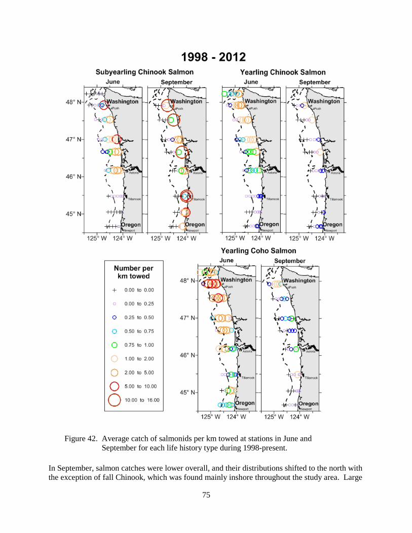
75

Figure 42. Average catch of salmonids per km towed at stations in June and

September for each life history type during 1998-present.

In September, salmon catches were lower overall, and their distributions shifted to the north with the exception of fall Chinook, which was found mainly inshore throughout the study area. Large

76

catches were consistently made at several stations along the La Push (48°N), Queets River (47.5°N) and Grays Harbor (47°N) transects, as well as at two stations associated with the plume: one 5 miles off Willapa Bay (46.6°N), and the other 7 miles off the mouth of the Columbia River (46.2°N).

Catches in both June and September were also very patchy in that we generally caught half of the fish in ~5% of the trawls per cruise and did not catch any fish in 40% of the trawls (Peterson et al. 2010). Patches most generally occurred for both yearling Chinook and coho off the Washington coast in June (Figure 42) and very near shore for yearling and subyearling Chinook in September.

Annual variation in salmon abundance—The lowest June catches of Chinook and coho salmon were associated with an El Niño event in 1998 and an anomalously low upwelling period during May-June 2005 (Figure 43). Conversely, the highest June catches occurred during years with a negative signal (cold phase) of the Pacific Decadal Oscillation (1999-2003 and 2008-2010). June 2012 catches were high for yearling Chinook salmon, but low for subyearling and mix-aged juvenile Chinook salmon and for yearling coho salmon.

Figure 43. Annual variation in catches of juvenile coho and Chinook salmon during June trawl surveys, 1998-present.

77

Introduction to Pacific Northwest Oceanography

Physical Oceanographic Considerations

The marine and anadromous faunae over which NOAA Fisheries exercises stewardship occupy diverse habitats in the coastal ocean off Washington, Oregon, and California. This biogeographic region has been collectively termed the Coastal Upwelling Domain (Ware and McFarlane 1989). Dominant fisheries species within this domain include market squid, northern anchovy, Pacific sardine, Pacific hake, Pacific mackerel, jack mackerel, Pacific herring, rockfish, flatfish, sablefish, and coho and Chinook salmon.

Within this domain, several smaller–scale physical zones are recognized, including:

(a) A near shore zone where juvenile fall Chinook salmon, sand lance, and smelts reside

(b) The upper 10–20 m of the water column across the continental shelf and slope, where many pelagic fishes reside, including juvenile coho and Chinook

(c) The benthic and demersal habitats on the continental shelf (English sole), at the shelf break (whiting, rockfish), and beyond the shelf break to depths of 1500 m (sablefish, Dover sole, and thornyheads)

Each of these physical zones has unique circulation patterns that affect spawning and larval transport, and each is subject to different physical conditions. These differing conditions lead to species–specific variations in growth, survival, and recruitment. Moreover, since many species have pelagic larvae/juvenile stages, recruitment is affected by broad–scale variation in both ocean productivity, which affects the feeding environment of larval and juvenile fish, and in ocean circulation, which affects the transport of eggs and larvae.

The Coastal Upwelling Domain is part of the California Current system, a broad, slow, meandering current that flows south from the northern tip of Vancouver Island (50°N) to Punta Eugenia near the middle of Baja, California (27°N). The California Current extends laterally from the shore to several hundred miles from land. In deep oceanic waters off the continental shelf, flows are usually southward all year round. However, over the continental shelf, flows are southward only in spring, summer, and fall: during winter, flow over the shelf reverses, and water moves northward as the Davidson Current.

These biannual transitions between northward and southward flow over the shelf occur in during March April and October November and are respectively termed the "spring transition" and "fall transition." Another important feature of circulation within the Coastal Upwelling Domain is the deep, poleward flowing undercurrent found year round at depths of 100–300 m over the outer shelf and slope. This current seems to be continuous from Southern California (33°N) to the British Columbia coast (50°N).

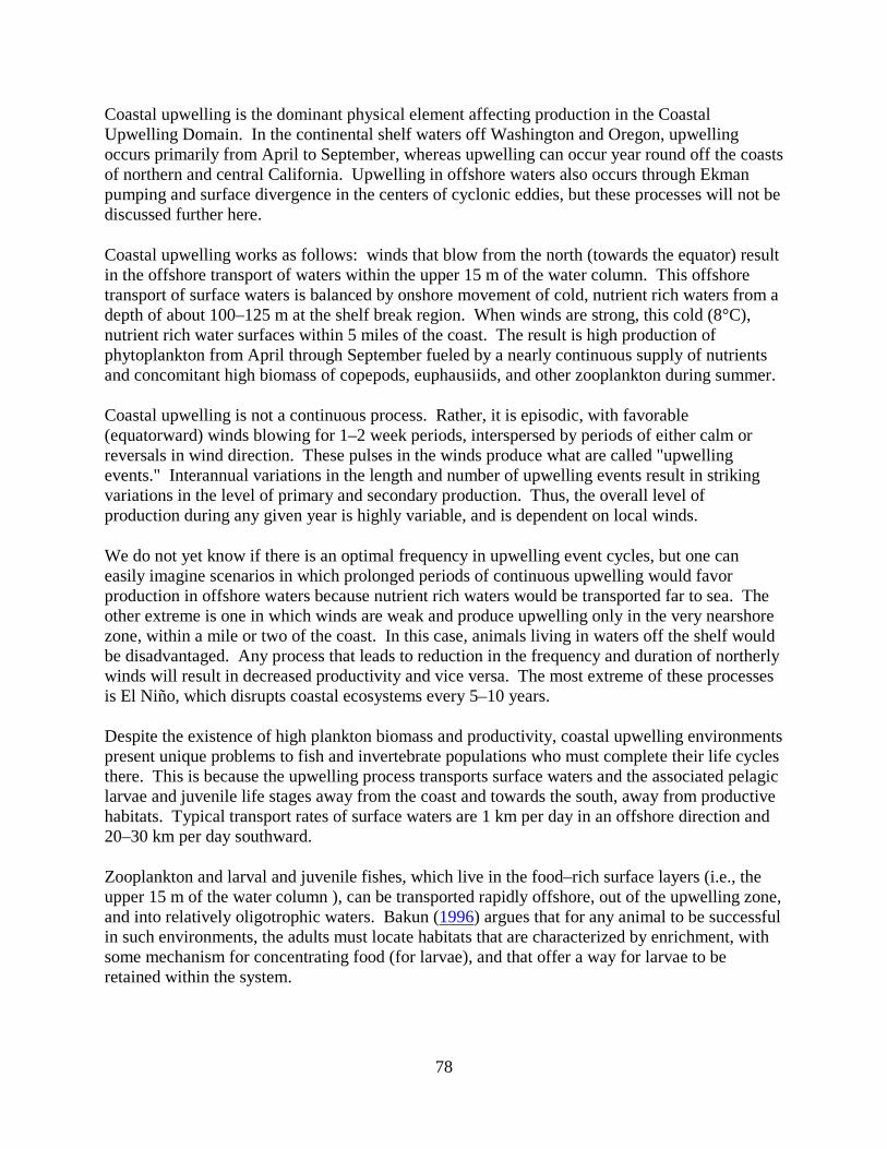
78

Coastal upwelling is the dominant physical element affecting production in the Coastal Upwelling Domain. In the continental shelf waters off Washington and Oregon, upwelling occurs primarily from April to September, whereas upwelling can occur year round off the coasts of northern and central California. Upwelling in offshore waters also occurs through Ekman pumping and surface divergence in the centers of cyclonic eddies, but these processes will not be discussed further here.

Coastal upwelling works as follows: winds that blow from the north (towards the equator) result in the offshore transport of waters within the upper 15 m of the water column. This offshore transport of surface waters is balanced by onshore movement of cold, nutrient rich waters from a depth of about 100–125 m at the shelf break region. When winds are strong, this cold (8°C), nutrient rich water surfaces within 5 miles of the coast. The result is high production of phytoplankton from April through September fueled by a nearly continuous supply of nutrients and concomitant high biomass of copepods, euphausiids, and other zooplankton during summer.

Coastal upwelling is not a continuous process. Rather, it is episodic, with favorable (equatorward) winds blowing for 1–2 week periods, interspersed by periods of either calm or reversals in wind direction. These pulses in the winds produce what are called "upwelling events." Interannual variations in the length and number of upwelling events result in striking variations in the level of primary and secondary production. Thus, the overall level of production during any given year is highly variable, and is dependent on local winds.

We do not yet know if there is an optimal frequency in upwelling event cycles, but one can easily imagine scenarios in which prolonged periods of continuous upwelling would favor production in offshore waters because nutrient rich waters would be transported far to sea. The other extreme is one in which winds are weak and produce upwelling only in the very nearshore zone, within a mile or two of the coast. In this case, animals living in waters off the shelf would be disadvantaged. Any process that leads to reduction in the frequency and duration of northerly winds will result in decreased productivity and vice versa. The most extreme of these processes is El Niño, which disrupts coastal ecosystems every 5–10 years.

Despite the existence of high plankton biomass and productivity, coastal upwelling environments present unique problems to fish and invertebrate populations who must complete their life cycles there. This is because the upwelling process transports surface waters and the associated pelagic larvae and juvenile life stages away from the coast and towards the south, away from productive habitats. Typical transport rates of surface waters are 1 km per day in an offshore direction and 20–30 km per day southward.

Zooplankton and larval and juvenile fishes, which live in the food–rich surface layers (i.e., the upper 15 m of the water column ), can be transported rapidly offshore, out of the upwelling zone, and into relatively oligotrophic waters. Bakun (1996) argues that for any animal to be successful in such environments, the adults must locate habitats that are characterized by enrichment, with some mechanism for concentrating food (for larvae), and that offer a way for larvae to be retained within the system.

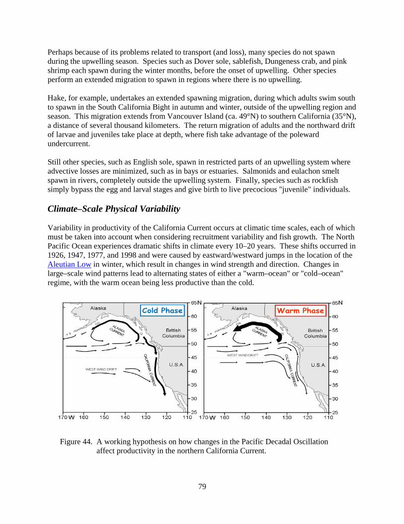
79

Perhaps because of its problems related to transport (and loss), many species do not spawn during the upwelling season. Species such as Dover sole, sablefish, Dungeness crab, and pink shrimp each spawn during the winter months, before the onset of upwelling. Other species perform an extended migration to spawn in regions where there is no upwelling.

Hake, for example, undertakes an extended spawning migration, during which adults swim south to spawn in the South California Bight in autumn and winter, outside of the upwelling region and season. This migration extends from Vancouver Island (ca. 49°N) to southern California (35°N), a distance of several thousand kilometers. The return migration of adults and the northward drift of larvae and juveniles take place at depth, where fish take advantage of the poleward undercurrent.

Still other species, such as English sole, spawn in restricted parts of an upwelling system where advective losses are minimized, such as in bays or estuaries. Salmonids and eulachon smelt spawn in rivers, completely outside the upwelling system. Finally, species such as rockfish simply bypass the egg and larval stages and give birth to live precocious "juvenile" individuals.

Climate–Scale Physical Variability

Variability in productivity of the California Current occurs at climatic time scales, each of which must be taken into account when considering recruitment variability and fish growth. The North Pacific Ocean experiences dramatic shifts in climate every 10–20 years. These shifts occurred in 1926, 1947, 1977, and 1998 and were caused by eastward/westward jumps in the location of the Aleutian Low in winter, which result in changes in wind strength and direction. Changes in large–scale wind patterns lead to alternating states of either a "warm–ocean" or "cold–ocean" regime, with the warm ocean being less productive than the cold.

Figure 44. A working hypothesis on how changes in the Pacific Decadal Oscillation

affect productivity in the northern California Current.

80

Changes in biological productivity are best documented for the period since the 1950s, and this understanding is largely due to measurements made by the California Cooperative Oceanic Fisheries Investigations (CalCOFI) program. Zooplankton biomass, for example, was high from the 1950s through 1977, but during the warm regime of 1977–1998, zooplankton biomass in the southern sector of the California Current declined by nearly one order of magnitude. In the northern California Current, the change in zooplankton biomass between regimes was not as dramatic, ranging just over one half an order of magnitude in coastal waters off Newport Orgeon. Zooplankton biomass was higher than average during the cool regime prior to 1977 and lower than average durring the warm regime from 1977 to 1998. During 2000–2004, zooplankton biomass rebounded to levels comparable to those seen prior to 1977.

Since the early 1980s, the California Current has been experiencing an increased frequency of El Niño events, with large El Niño events occurring every 5-6 years: 1976-77, 1982-83, 1986-87, 1991-92, 1997-98, 2002-03 and again in 2009-10. A higher frequency of El Niño events appears to be a characteristic of the extended periods of warm ocean conditions. From 1992 to 1998, the Oregon and Washington coasts experienced almost continuous El Niño-like conditions during summer (i.e., reduced upwelling and warmer ocean conditions). Since 1998, ocean conditions have improved markedly, and it appears that another regime shift may have been initiated in late 1998. Thus, the California Current now appears to have returned to a cool, productive phase. The shift to productive conditions was interrupted for 3 years (late 2002-late 2005), but the ocean once again cooled (in 2006). Whether or not short-term (3-4 year) variability will become the norm remains to be seen.

It is unclear why ENSO activity has a variable impact on the Pacific Northwest, but one problem is that we do not know precisely how ENSO signals are transmitted from the equator to the PNW. Signals can arrive through the ocean via Kelvin waves, which propagate up the coast of North America. ENSO signals can also be transmitted through atmospheric teleconnections. El Niño conditions can strengthen the Aleutian Low pressure system over the Gulf of Alaska; thus, adjustments in the strength and location of low pressure atmospheric cells at the equator can affect our local weather. This results in more frequent large storms in winter and disruption of upwelling winds in spring and summer. A summary of these interactions is available from NOAA's Earth Systems Research Laboratory.

We hypothesize that during "cold PDO" (such 1999–2002), a larger amount of water enters the California Current from the Gulf of Alaska, whereas during "warm PDO" such as 2003–2005, smaller amounts of water enter from the Gulf of Alaska and more enters from the North Pacific Current offshore or from the south. The changes in the type of source water yield the results shown in Table 8.

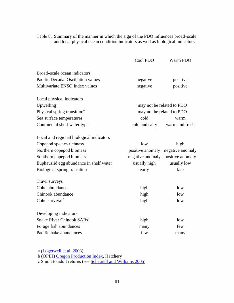
81

Table 8. Summary of the manner in which the sign of the PDO influences broad–scale

and local physical ocean condition indicators as well as biological indicators.

Cool PDO Warm PDO Broad–scale ocean indicators Pacific Decadal Oscillation values negative positive Multivariate ENSO Index values negative positive Local physical indicators Upwelling may not be related to PDO Physical spring transitiona may not be related to PDO Sea surface temperatures cold warm Continental shelf water type cold and salty warm and fresh Local and regional biological indicators Copepod species richness low high Northern copepod biomass positive anomaly negative anomaly Southern copepod biomass negative anomaly positive anomaly Euphausiid egg abundance in shelf water usually high usually low Biological spring transition early late Trawl surveys Coho abundance high low Chinook abundance high low Coho survivalb high low Developing indicators Snake River Chinook SARsc high low Forage fish abundances many few Pacific hake abundances few many a (Logerwell et al. 2003) b (OPIH) Oregon Production Index, Hatchery c Smolt to adult returns (see Scheurell and Williams 2005)

82

These simple relationships only hold during years of persistent recurrence of one phase of the PDO. During transitional years, such as 1998-1999, 2002-2003, and 2006-07, there are time lags in the ecosystem responses. For example, after the 1998 and 2002 climate shifts, water temperatures lagged the PDO by 1-2 months, changes in copepod biodiversity lagged the PDO index by 4-6 months, and changes in copepod biomass lagged the PDO by 2 years. Similarly, increases in abundances of forage fish and juvenile salmon lagged the PDO index changes by 1-2 years. The strongly negative "cool phase" PDO of 2008 yielded good returns of salmon (particularly coho) in 2009.

Acknowledgments

The contents of this page are derived from the efforts of many individuals. We thank the scientists and ship's crew who participated in the ocean sampling programs.

Special thanks to JoAnne Butzerin (NWFSC/FE; Technical Writing and Editing) for the initial design and editing, Justin Peters and Kevin Millikan (NWFSC/OMI) for the IT support.

Funding for data collection and data analysis came from the U.S. GLOBEC program NOAA–Center for Sponsored Coastal Ocean Research; grants NA 67RJ0151 and NA 86OP0589 and from the NOAA Fisheries and the Environment (FATE) Program.

Data collection was also supported by grants from the National Ocean Partnership Program (NA97FE0193), the National Science Foundation (9907854–OCE), and the Bonneville Power Administration .

83

References

Bakun, A. 1973. Coastal upwelling indices, west coast of North America, 1946–71. U.S. Department of Commerce, NOAA Technical Report NMFS–SSRF–671.

Bakun, A. 1996. Patterns in the ocean: ocean processes and marine population dynamics. University of California Sea Grant, La Jolla.

Beamish, R. J., and C. Mahnken. 2001. A critical size and period hypothesis to explain natural regulation of salmon abundance and the linkage to climate and climate change. Progress in Oceanography 49:423–437.

Bond, N. A., J. E. Overland, M. Spillane, and P. Stabeno. 2003. Recent shifts in the state of the North Pacific. Geophysical Research Letters 30(23):2183.

Bograd, S. J., I. Schroeder, N. Sarkar, X. Qiu, W. J. Sydeman, and F. B. Schwing. 2009. Phenology of coastal upwelling in the California Current. Geophys Res Lett 36.

Brodeur, R. D., E. A. Daly, C. A. Benkwitt, C. A. Morgan, and R. L. Emmett. In Press. Catching the prey: Sampling juvenile fish and invertebrate prey fields of juvenile coho and Chinook salmon during their early marine residence. Fisheries Research. doi:10.1016/j.fishres.2010.11.023

Brodeur, R. D., R.A. Schabetsberger, and K. L. Mier. 2007. Interannual and interdecadal variability in juvenile coho salmon diets in relation to environmental changes in the Northern California Current. Fisheries Oceanography 16:395-408.

Burke, B.J., Peterson, W.T., Beckman, B.R., Morgan, C., Daly, E.A., and Litz, M. 2013. Multivariate Models of Adult Pacific Salmon Returns. PloS one 8(1): e54134. DOI: 10.1371/journal.pone.0054134.

CDFG (California Department of Fish and Game). 2009. Report to the Fish and Game Commission: A status review of the longfin smelt (Spirinchus thaleichthys) in California. Internal report available at www.dfg.ca.gov (January 2010).

Columbia River DART (Data Access in Real Time). 1996—. Online interactive database of the Columbia Basin Research group, University of Washington School of Aquatic & Fishery Sciences. Available at www.cbr.washington.edu (September 2008).

Daly, E. A., R. D. Brodeur, and L. A. Weitkamp. 2009. Ontogenetic shifts in diets of juvenile and subadult coho and Chinook salmon in coastal marine waters: Important for marine survival? Transactions of the American Fisheries Society 138:1420–1438.

Emmett, R. L. 2006. The relationships between fluctuations in oceanographic conditions, forage fishes, predatory fishes, predator food habits, and juvenile salmonid marine survival off the Columbia River. Ph.D. Thesis, Oregon State University, Corvallis.

84

Emmett, R. L., S. L. Stone, S. A. Hinton, and M. E. Monaco. 1991. Distribution and abundance of fishes and invertebrates in West Coast estuaries, Volume II: Species life history summaries. Estuarine Living Marine Resources (ELMR) Report No. 8. NOAA/NOS, SEA Division, Rockville, MD.

Fessenden, L. M. 1996. Calanoid copepod diet in an upwelling system: phagotrophic protists vs. phytoplankton. Ph.D. Thesis, Oregon State University, Corvallis.

Gunsolus, R. T. 1978. The status of Oregon coho and recommendations for managing the production, harvest, and escapement of wild and hatchery–reared stocks. Oregon Department of Fish and Wildlife, Clackamas, OR.

Hart, J. L. 1973. Pacific Fishes of Canada. Fisheries Research Board of Canada, Bulletin 180:278–279.

Healey, M. C. 1991. Life history of Chinook salmon (Oncorhynchus tshawytscha). Pages 311–394 in C. Groot and L. Margolis, editors. Pacific salmon life histories. University of British Columbia Press, Vancouver.

Hooff, R. C., and W. T. Peterson. 2006. Copepod biodiversity as an indicator of changes in ocean and climate conditions of the northern California current ecosystem. Limnology and Oceaonography 51(6).

Logerwell, E. A., N. J. Mantua, P. W. Lawson, R. C. Francis, and V. N. Agostini. 2003. Tracking environmental processes in the coastal zone for understanding and predicting Oregon coho (Oncorhynchus kisutch) marine survival. Fisheries Oceanography 12(6):554–568.

Love, M. S., M. Yoklavich, and L. Thorsteinson. 2002. The rockfishes of the Northeast Pacific. University of California Press, London, UK.

Mantua, N. J., S. R. Hare, Y. Zhang, J. M. Wallace, and R. C. Francis. 1997. A Pacific decadal climate oscillation with impacts on salmon. Bulletin of the American Meteorological Society 78:1069–1079.

Matarese, A. C., A. W. Kendall, Jr., D. M. Blood, and B. M. Vinter. 1989. The rockfishes of the Northeast Pacific. Laboratory guide to the early life history stages of Northeast Pacific fishes. U.S. Deparment of Commerce, NOAA Technical Report NMFS 80.

Miller, C. B., H. P. Batchelder, R. D. Brodeur, and W. G. Pearcy. 1985. Response of the zooplankton and ichthyoplankton off Oregon to the El Niño event of 1983. Pages 185–187 in Worster, W. W., and D. L. Fluharty, editors. El Niño North. Washington Sea Grant Program, University of Washington, Seattle.

Myers, J. M., R. G. Kope, G. J. Bryant, D. J. Teel, L. J. Lierheimer, T. C. Wainwright, W. S. Grant, F. W. Waknitz, K. Neely, S. Lindley, and R. S. Waples. 1998. Status review of Chinook

85

salmon from Washington, Idaho, Oregon, and California. U.S. Department of Commerce, NOAA Technical Memorandum NMFS-NWFSC-35.

Nickelson, T. E. 1986. Influences of upwelling, ocean temperature, and smolt abundance on marine survival of coho salmon (Oncorhynchus kisutch) in the Oregon Production Area. Canadian Journal of Fisheries and Aquatic Sciences 43:527–535.

Pearcy, W. G. 1992. Ocean Ecology of North Pacific Salmonids. Washington Sea Grant Program, University of Washington Press, Seattle.

Peterson, W. T. 2009. Copepod species richness as an indicator of long–term changes in the coastal ecosystem of the northern California Current. California Cooperative Oceanic Fisheries Investigations (CalCOFI) Report 50:73-81.

Peterson, W. T., and J. E. Keister. 2003. Interannual variability in copepod community composition at a coastal station in the northern California Current: a multivariate approach. Deep Sea Research Part II: Topical Studies in Oceanography 50(14–16):2499–2517.

Peterson, W. T., and C. B. Miller. 1975. Year–to–year variations in the planktology of the Oregon upwelling zone. Fishery Bulletin, U.S. 73:642–653.

Peterson, W. T., and C. B. Miller. 1977. Seasonal cycle of zooplankton abundance and species composition along the central Oregon coast. Fishery Bulletin, U.S. 75:717–724.

Peterson, W. T., C. A. Morgan, J. P. Fisher, and E. Casillas. 2010. Ocean distribution and habitat associations of yearling coho (Oncorhynchus kisutch) and Chinook (O. tshawytscha) salmon in the northern California Current. Fisheries Oceanography 19(6):508-525.

PFMC (Pacific Fishery Management Council). 2011. Review of the 2010 Ocean salmon fisheries. PFMC, Portland, OR, February 2011. Available online at http://www.pcouncil.org/salmon/stock-assessment-and-fishery-evaluation-safe-documents/review-of-2010-ocean-salmon-fisheries/

Sandercock, F. K. 1991. Life history of coho salmon (Oncorhynchus kisutch). Pages 395–446 in C. Groot and L. Margolis, editors. Pacific salmon life histories. University of British Columbia Press, Vancouver.

Scheuerell, M. D., and J. G. Williams. 2005. Forecasting climate induced changes in the survival of Snake River spring/summer Chinook salmon (Oncorhynchus tshawytscha). Fisheries Oceanography 14(6):448–457.

Ware, D. M., and G. A. McFarlane. 1989. Fisheries production domains in the Northeast Pacific Ocean. Pages 359–379 in Beamish, R. J., and G. A. McFarlane, editors. Effects of ocean variability on recruitment and an evaluation of parameters used in stock assessment models. Canadian Special Publications of Fisheries and Aquatic Sciences 108.

86

Weitkamp L. A., T. C. Wainwright, G. J. Bryant, G. B. Milner, D. J. Teel, R. G. Kope, and R. S. Waples. 1995. Status review of coho salmon from Washington, Oregon, and California. U.S. Department of Commerce, NOAA Technical Memorandum NMFS-NWFSC-24.

Whiteaker, J. J., and K. Fryer. 2007. Age and length composition of Columbia Basin Chinook and sockeye salmon and steelhead at Bonneville Dam in 2006. Internal report. Columbia River Inter–Tribal Fish Commission 07–4.

Wolter, K., and M. S. Timlin. 1998. Measuring the strength of ENSO events: How does 1997/98 rank? Weather 53:315-324.

87

Glossary

Age Class Age at maturity, which may differ among fish of the same year class. For example, among wild Snake River spring Chinook born in 2003, 8% may mature as jacks, 73% after 2 years in the ocean, and 19% after 3 years.

Aleutian Low A semi–permanent, subpolar area of low pressure located in the Gulf of Alaska near the Aleutian Islands. It is a generating area for storms, and migratory lows often reach maximum intensity in this area. It is most active from late fall to late spring. During summer, it is weaker, retreating toward the North Pole and becoming almost nonexistent. During this time, the North Pacific High pressure system dominates (NOAA National Weather Service). Courtesy of NOAA National Weather Service.

California Current The California Current System (CCS) is a southward–flowing ocean current found along the west coast of North America, beginning at the northern tip of Vancouver Island, Canada, and ending near the southern tip of Baja California/Mexico. It is one of four elements of the anticyclonic North Pacific Gyre. The North Pacific Gyre includes the southward–flowing California Current, the westward–flowing North Pacific Equatorial Current (which flows toward Japan), the Kuroshio Current (which flows north along Japan) and the North Pacific Current (which flows eastwards towards North America).

CPUE We define catch per unit effort (CPUE) as the number of a particular species caught per kilometer traveled with the trawl under tow. However, CPUE is a relative and indirect measure of fishing effectiveness or species abundance. "Catch" can mean weight or numbers of total catch or of a particular species. "Units of effort" can be measured as individual cruises, the number of sets of a fishing net (or casts of a line), or as units of time or distance.

Geostrophic Wind A wind that is affected by Coriolis force, blows parallel to isobars and whose strength is related to the pressure gradient (i.e., spacing of the isobars). Courtesy of NOAA National Weather Service.

Escapement For salmon, the proportion of a population that returns as an adult to spawn in the natal stream (having "escaped" the catch in ocean fisheries).

Ichthyoplankton Ichthyoplankton are the eggs and larvae of fish. They are usually found in the sunlit zone of the water column, less than 200 meters deep, which is sometimes called the epipelagic or photic zone. Ichthyoplankton are planktonic, meaning they cannot swim effectively under their own power, but must drift with the ocean currents.

88

Jack A "Jack" is a male Chinook or coho salmon that returns to spawn prematurely, before growing to the size of a normal adult. Jacks stay in the ocean from a few months to a year, returning to the natal stream 1–2 years before normal adults of their age class. Thus numbers of returning jacks are sometimes used as a basis to predict run size the following year.

NH 05 A sampling station located 5 miles offshore along the Newport Hydrographic Line, a transect of established stations used in oceanographic sampling by NWFSC research teams since the mid-1970s (Figure 1). Findings at this station are often used as a reference point for ocean ecosystem indicator data.

Northern California Current The Northern California Current (NCC) is generally taken to be that part of the California Current that lies between the northern tip of Vancouver Island and the Oregon–California border, between Cape Blanco OR/Cape Mendocino CA. This portion of the CC shows a generally weak meandering flow year–round, which more–or–less flows parallel to the coast. It is characterized by strong seasonality in winds, upwelling, and biological productivity. Winter winds in the NCC are usually from the south or west, whereas summer winds are from the north and cause coastal upwelling.

North Pacific High The North Pacific High pressure system is the region of high sea-level pressure that occurs over the eastern North Pacific Ocean in the climatological mean as shown in Figure 1 (Mass and Bond 1996).icon

Oblique Tow A tow made by pulling the net at a slow tow speed from the sea floor to the surface. Under this configuration, the angle between the net and sea floor is maintained at 45 degrees.

OPIH (Oregon Production Index, Hatchery) For coho, an estimate of total freshwater escapement, adjusted for ocean and freshwater catch, for public hatchery fish throughout the Oregon Production Index Area. Private hatchery production is removed from this estimate, so it reflects only public hatchery fish. Used as the numerator in calculating SARs for the OPIH.

Recruitment Number or proportion of biomass added to a fish population as a result of growth or reproduction, especially for a given year class.

Secchi Disk A device to measure the turbidity (transparency) of the upper water column. A 30–cm diameter white disc is lowered slowly through the upper water column to the point at which the pattern is no longer visible. The depth of the disk is then taken as a measure of transparency or turbidity.

89

SAR (smolt–to–adult ratio) For a population of salmon, the number from a given year class that survived to the smolt stage (i.e., migrated as juveniles) divided by the total number of returning adults from that year class (all age classes combined).

Teleconnection The term "teleconnection pattern" refers to a recurring and persistent, large–scale pattern of pressure and circulation anomalies that spans vast geographical areas. Teleconnection patterns are also referred to as preferred modes of low–frequency (or long time–scale) variability. Courtesy of the NOAA National Weather Service Climate Prediction Center.

Transmissometer A device for measuring beam attenuation, which can be used as a measure of turbidity in water. A beam of light is cast through the water and the transmissometer records the measure of light at a given point past the source of the beam.

Year Class Fish of the same species and stock that are born in the same year.