ocean color science working group highlights - … geo‐cape workshop aug. 31‐sept. 2, 2015 •...

Ocean Color Science Working Group Highlights

Antonio Mannino

NASA GSFC

GEO‐CAPE Workshop Aug. 31‐Sept. 2, 2015

https://ntrs.nasa.gov/search.jsp?R=20150020465 2018-06-26T21:06:19+00:00Z

2

GEO‐CAPE Oceans Activities Science Working Group Activities Science Traceability Matrix Applications Traceability Matrix Science Value Matrix DevelopmentWhite Papers PI‐led scientific investigations Field Campaigns

• Chesapeake Bay ‐ July 2011 (CBODAQ)• Gulf of Mexico Experiment ‐ September 2013 (GoMEX)• Korean coastal waters ‐May‐June 2016 (KORUS‐OC) ‐ joint w/ KIOST

Recent Engineering Studies 2011 Pointing Study 2014 Instrument Cost vs Capability study 2015‐2016 Functional 50‐band filter wheel breadboard 2015 Scheduling Study

Outreach

Outline


• Activities to develop a Science Value Matrix• Recent updates to Science Traceability Matrix• Instrument capability vs cost study• Filter wheel mechanism breadboard study• Pointing study• Scheduling study• Gulf of Mexico field campaign • Other Science Studies• NASA Earth Science Applied Sciences Program discussion• Applications Science Matrix • Outreach: Ocean Optics Town Hall, update at OCRT, IOCS

breakout session and poster, CERF 2015 town hall planned• Pre‐Decadal Survey Activities• How to sell the mission?

Science Value Matrix 0 2 4 6 8

10

12

Nearshore Coastal Regions OC

HABs Detec on

River Fluxes

Diurnal Produc vity

Highly Turbid Coastal Waters OC

Phytoplankton Taxonomy

Con nental Margin OC

HABs Quan fica on

Estuarine & Coastal Circula on

Diurnal Phytoplankton Physiology

Atm. Correc on (Abs. aerosols & NO2)

Diurnal Photooxida on

Surface water flow rate & direc on

Petroleum Detec on & Quan fica on

Diurnal Turnover of Carbon

Detec on of Fronts, Mesoscale Eddies,

Larger Inland water bodies >1km OC

Dust Transport

Open Ocean OC

Small Inland water bodies <1km OC

Median Score

• Based on these Median scores it is recommended that the GEO‐CAPE ocean color instrument be designed to address applications with a score of 8 or higher.

• Applications that scored 7 should be adequately addressed by this same instrument.

• Dust transport will also be measured for the areas sampled.

• Open ocean OC requires additional area sampling and duplicates sampling with other instruments.

• This instrument will not have adequate spatial resolution for small inland water bodies.

Science Application Priorities

Science Value Activity Recommendations• Spatial resolution

• continue trade between 375 m (Threshold) and 250 m GSD (Baseline) at Nadir• Temporal resolution

• Hourly for Targets and US coastal waters (including Great Lakes)• UV Radiometry 340‐400 nm• SWIR bands 1245 and 1640 nm

• Alternate SWIR bands are very low priority and no longer considered• Spectral capability ‐ NO CONSENSUS YET

• Proposed: Hyperspectral 340‐1050 nm (2‐5 nm) (New Baseline) vs. 50 band Multispectral (5 nm bands) (New Threshold)

• Spectral sampling 2‐5 nm plus 0.4 to 0.8 nm over 400‐450 nm for NO2• Coastal coverage 375 km from inland to offshore for US coastal waters survey • SNR >1000:1 for 350‐ 800 nm binned to 10 nm FWHM (combines UV and visible)

Recommend updating STM to reflect these priorities and the remaining trades and then review current instrument designs in light of these new requirements.

SWG should discuss whether to update STM to reflect results and then review current instrument designs.

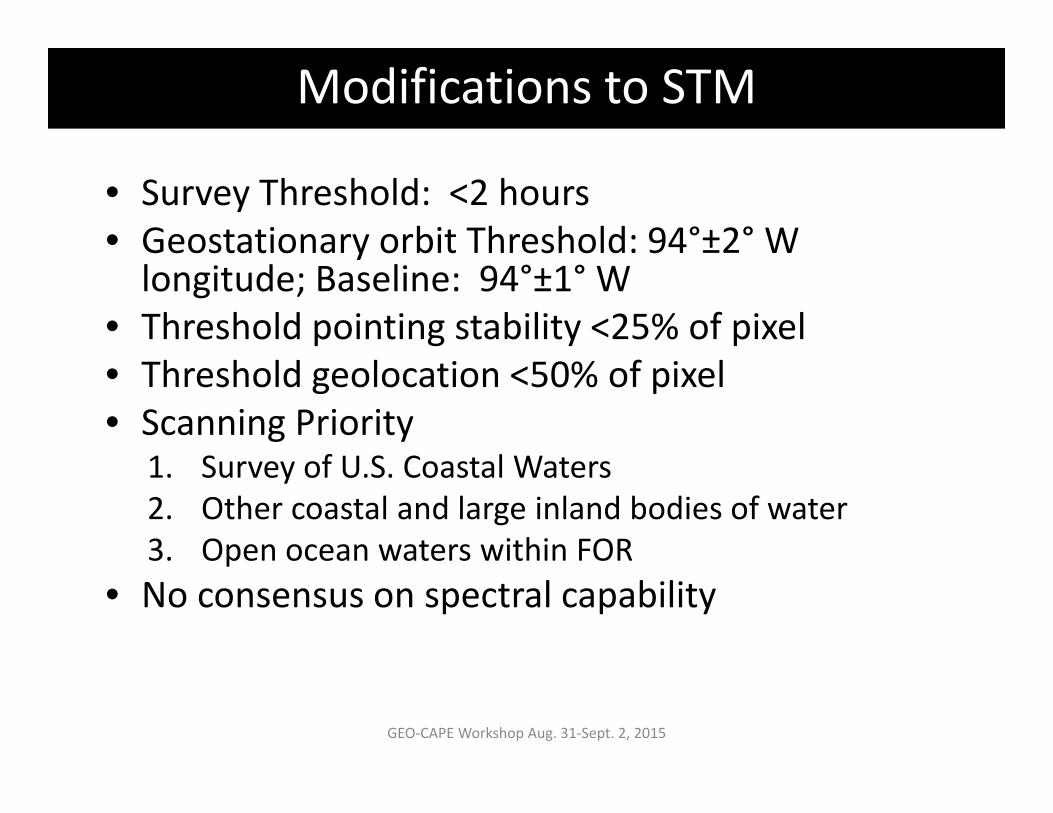
Modifications to STM


• Survey Threshold: <2 hours• Geostationary orbit Threshold: 94°±2° W longitude; Baseline: 94°±1° W

• Threshold pointing stability <25% of pixel• Threshold geolocation <50% of pixel• Scanning Priority

1. Survey of U.S. Coastal Waters2. Other coastal and large inland bodies of water3. Open ocean waters within FOR

• No consensus on spectral capability

Threshold (minimum) Baseline (goal)

Temporal ResolutionTargeted Events <1 hour <0.5 hourSurvey Coastal U.S. <2 hours <1 hour

Spatial Resolution (nadir) 375 m x 375 m 250 m x 250 m

Spectral Range 345‐1050 nm; 2 SWIR bands 1245 & 1640 nm

340‐1100 nm; 3 SWIR bands 1245, 1640, 2135 nm

Scan Rate >25,000 km2/min >50,000 km2/min

Spectral ResolutionUV‐VIS‐NIR: ≤5 nm;

400‐450nm: ≤0.8nm (NO2); SWIR: ≤20‐40 nm

UV‐VIS: ≤0.75 nm; SWIR: ≤20‐50 nm

Signal‐to‐Noise Ratio (SNR)@ Ltyp for 70° solar zenith angle

1000:1 for 350‐800 nm (10nm FWHM);

600:1 for NIR (40nm FWHM); 250:1 & 180:1 for 1245 & 1640 nm (20 &

40nm FWHM); ≥500:1 NO2

1500:1 for 350‐800 nm;

100:1 for 2135nm (50nm FWHM); NIR, SWIR and NO2

same as threshold

Measurement & Instrument Requirements

9

Competing Technical ChallengesChallenge: achieving an engineering solution for requirements that are in opposition to each other• Spatial resolution• Temporal resolution• Spectral resolution• Hyperspectral

Instrument concepts• Filter radiometer (GOCI)• Single slit spectrometer• Multi‐slit spectrometer• Wide Field‐of‐View spectrometer

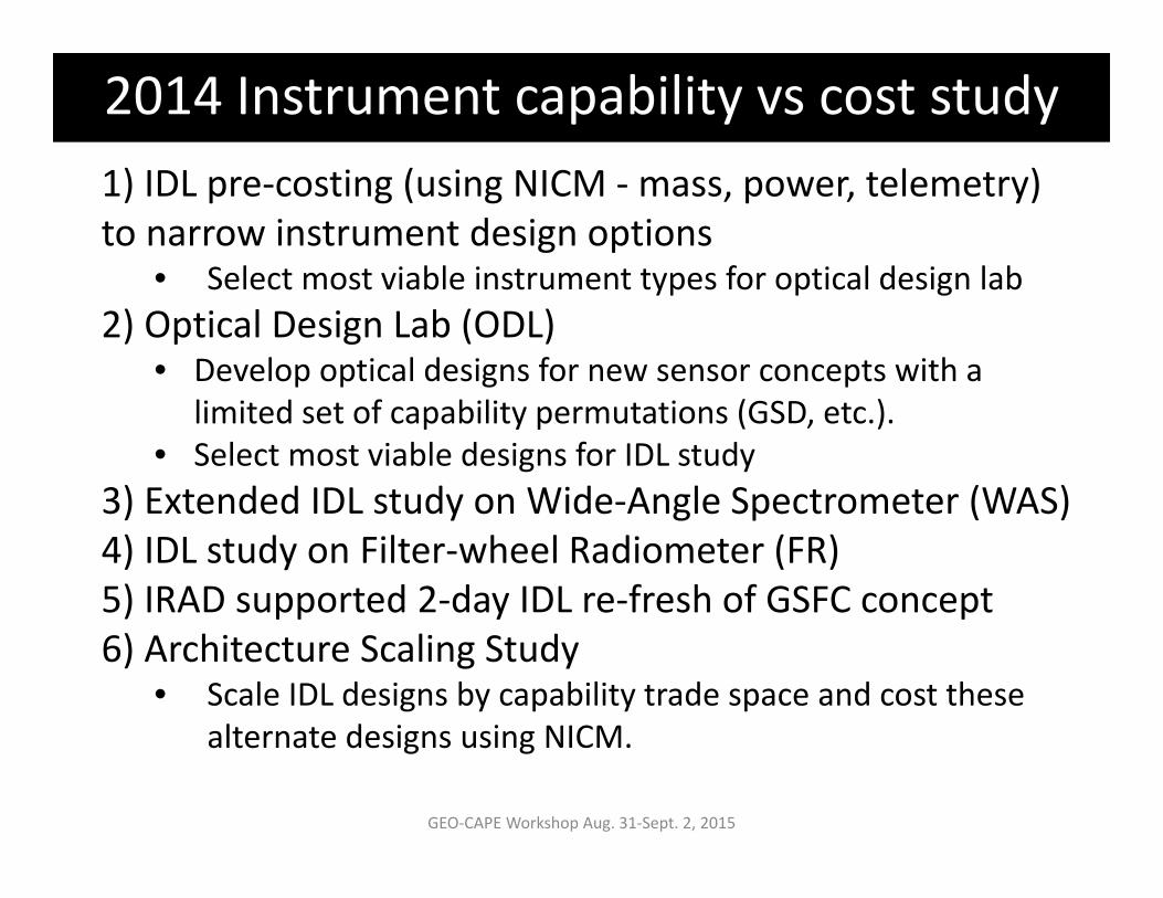
2014 Instrument capability vs cost study


1) IDL pre‐costing (using NICM ‐mass, power, telemetry) to narrow instrument design options

• Select most viable instrument types for optical design lab2) Optical Design Lab (ODL)

• Develop optical designs for new sensor concepts with a limited set of capability permutations (GSD, etc.).

• Select most viable designs for IDL study3) Extended IDL study on Wide‐Angle Spectrometer (WAS)4) IDL study on Filter‐wheel Radiometer (FR)5) IRAD supported 2‐day IDL re‐fresh of GSFC concept6) Architecture Scaling Study

• Scale IDL designs by capability trade space and cost these alternate designs using NICM.

Input to Pre‐costing ‐ 2011 Informal RFI


RaytheonGLIMR

RaytheonGOI

Ball MOS

GSFCCOEDI

JPLCOCOA

GSFC CEDIIDL Jan. 2010

GSD at nadir (m) 250 x 250 225 x 225 375 x 375 375 x 375 200 x 200 375 x 375

Spectral Range (multi- or hyper-spectral)

340-885 980-2200

340-885 980-2200

340-900 SWIR bands

340-1100 SWIR bands

350-1050 nm

340-1100 1.2-2.5

Spectral sampling & resolution (nm)

~5nm (HS) SWIR 20-50

~5nm (HS) SWIR 20-50

~5 nm

~0.4/0.8 nm SWIR 20-40

<5 nm multi-

spectral

0.5 nm SWIR – 5

iFOV (E/W x N/S pixels) 1 x 8192 1 x 8192 1 x 2048 1 x 2048 2048 x 2048

1 x 2048

iFOV Stare Interval 4 sec 0.9 sec 4 sec 0.8 sec 0.2 sec 0.8 sec

SNR 1000 required

@443nm; 10nm FWHM; Ltyp = 45 W m-2 um-1 sr-1

2310 2500 2320 1748 1000 2148

@678nm; 10nm FWHM; Ltyp=8.66 W m-2 um-1 sr-1

1150 1200 1866 1031 800 1195

Time to scan 3x105 km2 @ SNR & Ltyp listed above Scan Rate (km2 min-1)

26.4 min

11,364

10.9 min

27,523

6.1 min

49,180

17.36 min

17,281

11.96 min

25,084

17.8 min

16,854 Geo design life (years) 3 3 3 3 2 3 Power CBE 360 W 390 W 220 W 50 W 392 W Size CBE (length x width x height)

0.7 x 0.6 x 0.8 m 1.7 x 1.5 x 2.0 m

1.5 x 1.5 x 1.7 m

1.5 x 1.7 x 1.1 m

Cylinder 0.9m dia. x 1.3 m

2.1 x 0.95 x 2.8 m

Mass CBE (kg) 132 kg 283 kg 147 kg 220 kg 71 kg 548 kg Thanks to Jeff Puschell (Raytheon), Tim Valle & Paula Wamsley (Ball), Richard Key (JPL)

2014 Instrument capability vs cost study


HyperspectralSpectrometers

Multi-spectral Filter Radiometer

InstrumentType

Single Slit, Multi-slit, Wide-Angle

Filter Wheel Instrument

Spatial Resolution 250, 375 & 500 m 250, 375 & 500 m

SpectralResolution 0.4 and 2 nm 5 nm

Spectral Range 340-1050 nm 50 bands: 340-1050

SWIR Bands 1245, 1640, 2135 nm 1245, 1640, 2135 nm

SNR (UV-Vis; 10 nm bands) 1000 1000

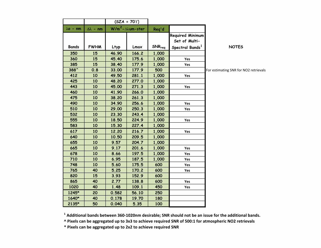
λo - nm - nm Req'd

Bands FWHM Ltyp Lmax SNRreq

Required Minimum Set of Multi-

Spectral Bands1 NOTES350 15 46.90 166.2 1,000360 15 45.40 175.6 1,000 Yes385 15 38.40 177.9 1,000 Yes388^ 0.8 33.00 177.9 500 For estimating SNR for NO2 retrievals412 10 49.50 281.1 1,000 Yes425 10 48.20 277.0 1,000443 10 45.00 271.3 1,000 Yes460 10 41.90 266.0 1,000475 10 38.20 261.3 1,000490 10 34.90 256.6 1,000 Yes510 10 29.00 250.3 1,000 Yes532 10 23.30 243.4 1,000555 10 18.50 224.9 1,000 Yes583 10 15.30 227.4 1,000617 10 12.20 216.7 1,000 Yes640 10 10.50 209.5 1,000655 10 9.57 204.7 1,000665 10 9.17 201.6 1,000 Yes678 10 8.66 197.5 1,000 Yes710 10 6.95 187.5 1,000 Yes748 10 5.60 175.5 600 Yes765 40 5.25 170.2 600 Yes820 15 3.93 152.9 600865 40 2.77 138.8 600 Yes1020 40 1.48 109.1 450 Yes1245* 20 0.582 56.10 2501640* 40 0.178 19.70 1802135* 50 0.040 5.35 100

1 Additional bands between 360‐1020nm desirable; SNR should not be an issue for the additional bands.^ Pixels can be aggregated up to 3x3 to achieve required SNR of 500:1 for atmospheric NO2 retrievals * Pixels can be aggregated up to 2x2 to achieve required SNR

(SZA = 70)

W/m2-∆λum-ster

2014 Instrument Study Cost Assumptions


• 1 Flight Unit and Engineering Development Unit through PRICE‐H• Engineering Test Units (ETUs) (10% of FU cost) and Component Spares

covered by wrap factors• Class C Mission (selective redundancy)

• (Class B Parts – up‐screening not included in cost estimate)• 3 year design life (5‐yr goal)• Costs reported in FY2016 constant year dollars• Instrument built by contractor • Flight Software (FSW) Estimated using GSFC in‐House bid rates• SEER‐H cost estimates for Detectors• Schedule used: ATP: 12/17, CDR: 12/18, PER: 5/21; Launch 12/2023• IDL study costs included HW and firmware to compensate for jitter and

roll (star tracker, gyro, fast‐steering mirror, passive struts, actuators and roll camera)

• IDL provides instrument point design concepts with cost confidence level of 20‐30% (rule of thumb to multiply by 1.5 to increase CL to 70%)• NICM system and sub‐system versions provide 50% CL

15

Instrument Relative SizeWide‐Angle Spectrometer (WAS) ‐ 375m GSD

Coastal Ecosystems Dynamics Imager (COEDI) ‐ 375m GSD

GSFCProprietary

Filter Radiometer (FR) ‐ 250m GSD

16

Spectral resolution: 0.4, 2, 5 nmNadir GSD: 250, 375, 500 mSWIR: 3 bands

Instrument capability vs cost study

WAS = Wide Angle SpectrometerFR = Filter Radiometer SSS = single‐slit spectrometerCOEDI = dual slit spectrometer (GSFC)GLIMR = wide angle spectrometer (Raytheon)MOS = 4‐slit spectrometer (Ball)GOCI = Korean/Astrium filter radiometer (360m)

Instrument Capability vs Cost

Instrument Type Filter Radiometer FR

Wide Angle Spectrometer

WAS

Multi‐Slit Spectrometer COEDI

Spatial Resolution 250 m 375 m 375 m 375 m 250 mSpectral Resolution 5 nm 5 nm 0.4 nm 0.4 nm 0.4 nm

Spectral Range (nm)(2135 not req)

Multispectral (50) 340‐1050;

1245, 1640, 2135

Multispectral(50) 340‐1050;

1245, 1640, 2135

340‐1050;1245, 1640, 2135

nm

340‐10501245,1640 nm

340‐10501245,1640 nm

Scan Rate (km2/min) 100,105 100,105 48,200 43,200 28,800

Mass CBE (kg) 190.4 126.3 309.4 202.8 358.6

Power CBE (W) 200.1 161.2 341.3 192.5 257.7

Volume (m x m x m) 1.5 x 1.46 x 1.02 1.0 x 0.97 x 0.68 2.6 x 1.8 x 1.5 1.5 x 1.7 x 1.1 2.2 x 2.5 x 1.7

Telemetry CBE (kbps) 15,900 10,600 23,832 23,854 35,765

NICM Cost ($M) $213.4 $172.9 $325.2 $238.8 $308.0

Parametric Cost ($M) $131.7 $107.7 $165.2 $136.2 $200.1

NICM Sub‐System Cost ($M) $128.7 $179.3


Cost Estimate for Ocean Color GEO-CAPE

WBS Element Cost Cost ($M)

Instrument $133M * 1.5 200

Project Mngmt, Sys. Engr., & SMA* 10%* 60

Ground Sys. & Mission Ops.* 13%* 45

Host Fees (I&T, Launch, Data) TBD 80

Science 65

Reserves 10% 45TOTAL $495M

* Cost % from recent LEO missions (should be lower for hosted mission)

GEO‐CAPE Workshop Aug. 31‐Sept. 2, 2015 19

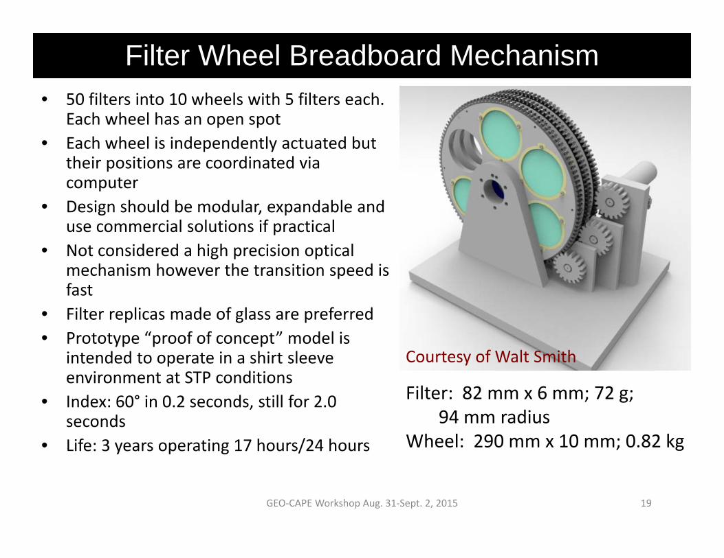
Filter Wheel Breadboard Mechanism

Filter: 82 mm x 6 mm; 72 g; 94 mm radius

Wheel: 290 mm x 10 mm; 0.82 kg

• 50 filters into 10 wheels with 5 filters each. Each wheel has an open spot

• Each wheel is independently actuated but their positions are coordinated via computer

• Design should be modular, expandable and use commercial solutions if practical

• Not considered a high precision optical mechanism however the transition speed is fast

• Filter replicas made of glass are preferred • Prototype “proof of concept” model is

intended to operate in a shirt sleeve environment at STP conditions

• Index: 60° in 0.2 seconds, still for 2.0 seconds

• Life: 3 years operating 17 hours/24 hours

Courtesy of Walt Smith

• Spacecraft attitude control rejects low‐frequency disturbances (≤ 0.1 Hz)

• Jitter suppression system on instrument mount rejects high‐frequency disturbances (1.5 Hz and above)

Low Frequency (Attitude Control)

Mid Frequency (Fast Steering)

High Frequency (Isolation)

0.1 Hz 1.5 Hz

Disturbance Rejection Apportioned by Frequency

• Active elements, plus passive rolloff due to inertia• Active “fast steering loop” rejects mid‐frequency disturbances (0.1

to 1.5 Hz)• Needs IMU sampled at >15 Hz• Actuation by either:

• A fast steering mirror (baseline), or • By steering the scanning mirror, or• Active portion of the jitter suppression system

Courtesy of Eric Stoneking

FY15 Scheduling Study


Study Aims• Optimize Acquisition of “Cloud Free” Scenes at Lowest Cost• Scheduling of observations based on science priorities and cloud

coverNASA Ames Activities

Jeremy Frank et al.• Scene Layouts for FR and COEDI sensors (STK analysis)

• GSD determination across sensor view angles• Automated scheduler

• Requires cloudiness predictions, cloudiness thresholds, scenes• Evaluation of automation technologies

GSFC study Elements ‐ http://geocape.herokuapp.comKaren Moe, Dan Mandl, Jacqueline LeMoigne, Stuart Fry & Pat Cappelaere

• Smart cloud forecasting• On‐board cloud detection• Ground/on‐board scheduling with Robust Executive

21

Strawman 18 Coastal/Lakes Survey Scenes Using FR

Source: GSFC analysis via GUI Editor, assuming spherical Earth – Satellite at 95W

~45min to scan CONUS coastal waters

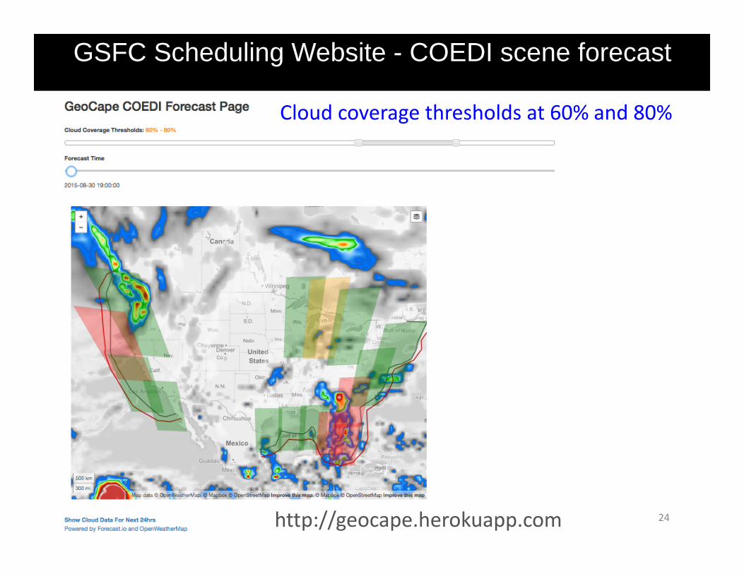
SURVEY SCENES & FORECAST

Example FR Scene Forecast showing:

Red scenes fail cloud threshold and are not scheduled

Green scenes pass cloud threshold and are scheduled

Orange scenes are marginal and are scheduled for more evaluation onboard

GEO‐CAPE Workshop Aug. 31‐Sept. 2, 2015 24

GSFC Scheduling Website - COEDI scene forecast

Cloud coverage thresholds at 60% and 80%

http://geocape.herokuapp.com

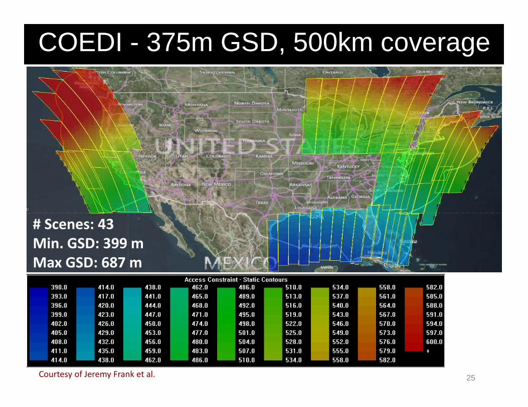
COEDI - 375m GSD, 500km coverage

25Courtesy of Jeremy Frank et al.

# Scenes: 43Min. GSD: 399 mMax GSD: 687 m

FR - 250 m GSD

26

# Scenes: 38Min. GSD: 399 mMax GSD: 701 m

Courtesy of Jeremy Frank et al.

Min. GSD: 262 mMax GSD: 295 m

27

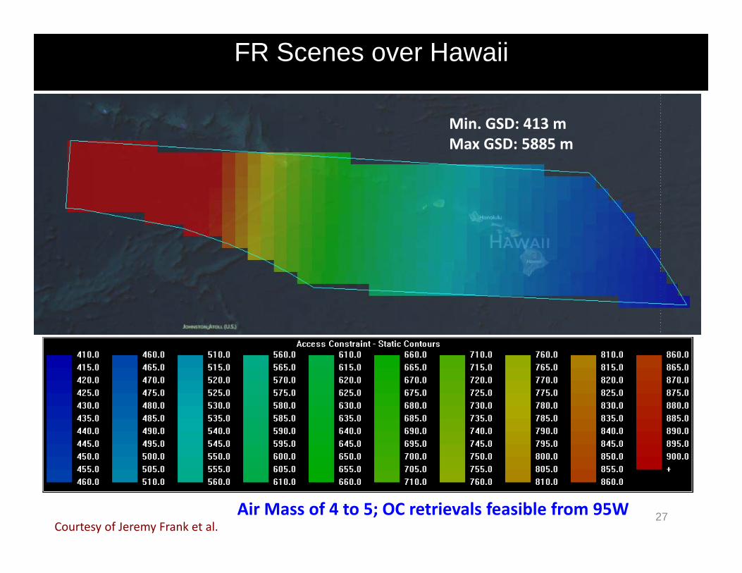
Min. GSD: 413 mMax GSD: 5885 m

FR Scenes over Hawaii

Courtesy of Jeremy Frank et al.Air Mass of 4 to 5; OC retrievals feasible from 95W

Gulf of Mexico Experiment ‐ Sept. 2013


14-day oceanographic & atmospheric properties•Transects along gradients

• nearshore to offshore, river plumes, algal bloom patches• addresses aquatic & atmospheric spatial variability

• Tracking water masses (follow instrumented drogue)• diurnal evolution of biology & biogeochemistry

• Small boat operations (more optically complex waters)• Marsh Island area; Galveston & Trinity Bay

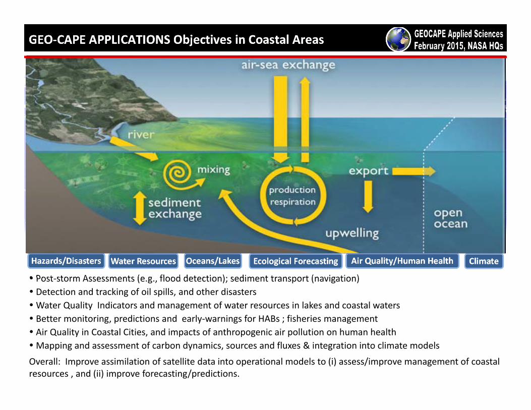
GEO‐CAPE APPLICATIONS Objectives in Coastal Areas

Post‐storm Assessments (e.g., flood detection); sediment transport (navigation) Detection and tracking of oil spills, and other disasters Water Quality Indicators and management of water resources in lakes and coastal waters Better monitoring, predictions and early‐warnings for HABs ; fisheries management Air Quality in Coastal Cities, and impacts of anthropogenic air pollution on human healthMapping and assessment of carbon dynamics, sources and fluxes & integration into climate models

Overall: Improve assimilation of satellite data into operational models to (i) assess/improve management of coastal resources , and (ii) improve forecasting/predictions.

MERIS: Amazon Delta, Northern Brazil 01. October 2005, orbit: 18758MERIS: Sediments , Amazon Delta, Northern Brazil 01. October 2005Bangladesh coastline, flooding‐Ganges transports sediments, MERIS, March 2005 Oil Spill, Mississippi Delta, MODIS‐Terra, March 24, 2010

MODIS/Terra,

4/29/2010, 16:55 GMT

MODIS/Aqua,

4/29/2010, 18:30 GMT

MODIS images just 1.5 hours apart, yet showing changes in the oil appearance and location (from Fishman et al. (2012).

This image cannot currently be displayed.

Algae in Lake Erie, MODIS‐Terra, Rapid Response, March 21, 2012Red tides in Benguela upwelling, Aerial photo Pitcher et al., Oceanogr. 2008 GOCI‐observed diurnal changes of a harmful algal bloom of Prorocentrum donghaiense along the East China’s coast. From Lou and Hu (2014).

Hazards/Disasters Water Resources Oceans/Lakes Ecological Forecasting ClimateAir Quality/Human Health

30

Agency Applications Satellite products Spatial requirements

Temporal requirements

NOAA Habitat assessment, fisheries management, water quality, HABS, ecological forecasting, pollution monitoring, coral health, acidification

Chlorophyll, Rrs(λ), abs(λ), HABs, K490, KPAR

100m – 4km 3hrs ‐ daily

EPA Sustainable coastal resources; air, climate and energy research; healthy and sustainable coastal communities

Chlorophyll, Rrs(λ), abs(λ), abs(cdom, phy, det), HABs, SPM, K490, KPAR and more

<250m to 500m

0.5 hrs – 3hrs

US Navy Surface currents, instrument assessments, bathymetry, visibility, coastal oceanography, navigation

Chlorophyll, Rrs(λ), abs(λ), abs(cdom, phy, det), bbp(λ), HABs, SPM, K490, KPAR currents, etc.

250m – 1km 1hr ‐ daily

Gulf of Mexico Fishery MgmtCouncil

Habitat quality, fisheries conservation, coral conservation

Chlorophyll, NPP, currents Not specified

Not specified

BOEM Ecological models, sediment transport, current trajectory, oil detection and thickness

Chlorophyll, NPP, currents, cdom, SPM

Not specified

Not specified

U.S. Army Corps of Engineers

Coastal & Inland Water Quality Monitoring and Forecasting (including HAB detection and monitoring), Nearshore Benthic Habitat Mapping to Support Coastal Operations and Planning

Chl‐a, phycocyanin, CDOM, turbidity, CDOM, green laser reflectance, hyperspectral Rrs, bottom type characterization, habitat change detection

5 to 50 m daily (WQ), monthly-seasonal (mapping)

Applications Traceability Matrix

Applications Identified• Habitat Quality/Assessment/Mapping• Water Quality• Fisheries Management• Ecological Models• Ecological Forecasting• Sustainability• Research• Human Health• Pollution Tracking• HABs• Current Trajectory• Visibility• Sustainability

31

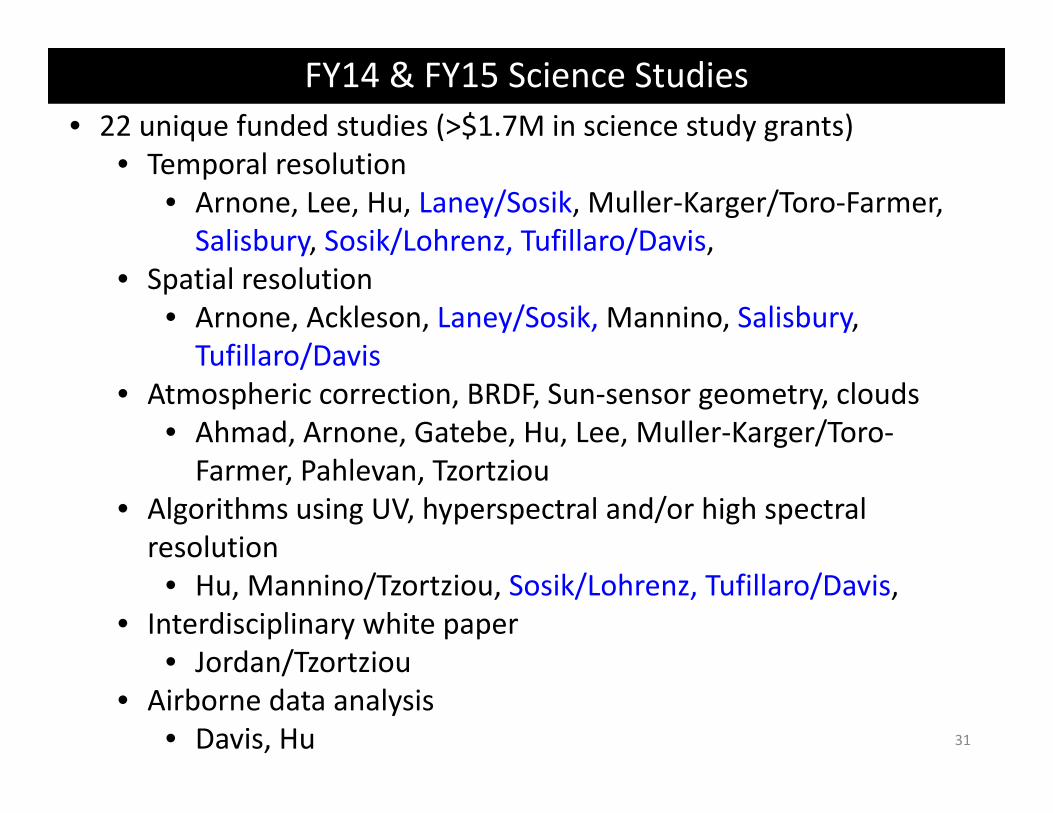
FY14 & FY15 Science Studies• 22 unique funded studies (>$1.7M in science study grants)

• Temporal resolution • Arnone, Lee, Hu, Laney/Sosik, Muller‐Karger/Toro‐Farmer, Salisbury, Sosik/Lohrenz, Tufillaro/Davis,

• Spatial resolution • Arnone, Ackleson, Laney/Sosik, Mannino, Salisbury, Tufillaro/Davis

• Atmospheric correction, BRDF, Sun‐sensor geometry, clouds• Ahmad, Arnone, Gatebe, Hu, Lee, Muller‐Karger/Toro‐Farmer, Pahlevan, Tzortziou

• Algorithms using UV, hyperspectral and/or high spectral resolution

• Hu, Mannino/Tzortziou, Sosik/Lohrenz, Tufillaro/Davis, • Interdisciplinary white paper

• Jordan/Tzortziou• Airborne data analysis

• Davis, Hu

Beyond PACE: Future Measurements for Coastal and Applications Research

Detection and tracking of red tides in coastal waters

Coastal Phytoplankton Dynamics

Biogeochemical processes in coastal waters

Detection & Tracking of Oil Spill

Harmful Algal blooms & water quality in inland waters

Sediment transport

Link data to models and decision‐support tools and processes (e.g., predict hypoxic regions, fisheries mngmt, ocean acidification, water‐quality forecasting)

33

Outreach• Splinter session on geo ocean color & presentation on GEO‐CAPE at International Ocean Color Science Meeting (May 2013)

• NASA Ocean Color Research Team Meeting (May 2014)• Ocean Optics Conference Town Hall (Nov. 2014)• HyspIRI Meeting (June 2015)• NASA OCRT update (June 2015)• International Ocean Color Science Meeting (June 2015)

• Breakout session on geo ocean color & presentation on GEO‐CAPE

• Planned Town Hall at CERF (Nov. 2015)

34

How to sell the mission to stakeholders?

• Ecosystem Health Index• Global constellation of Geo ocean color• Synergy with PACE and other OC missions• Synergy with TEMPO

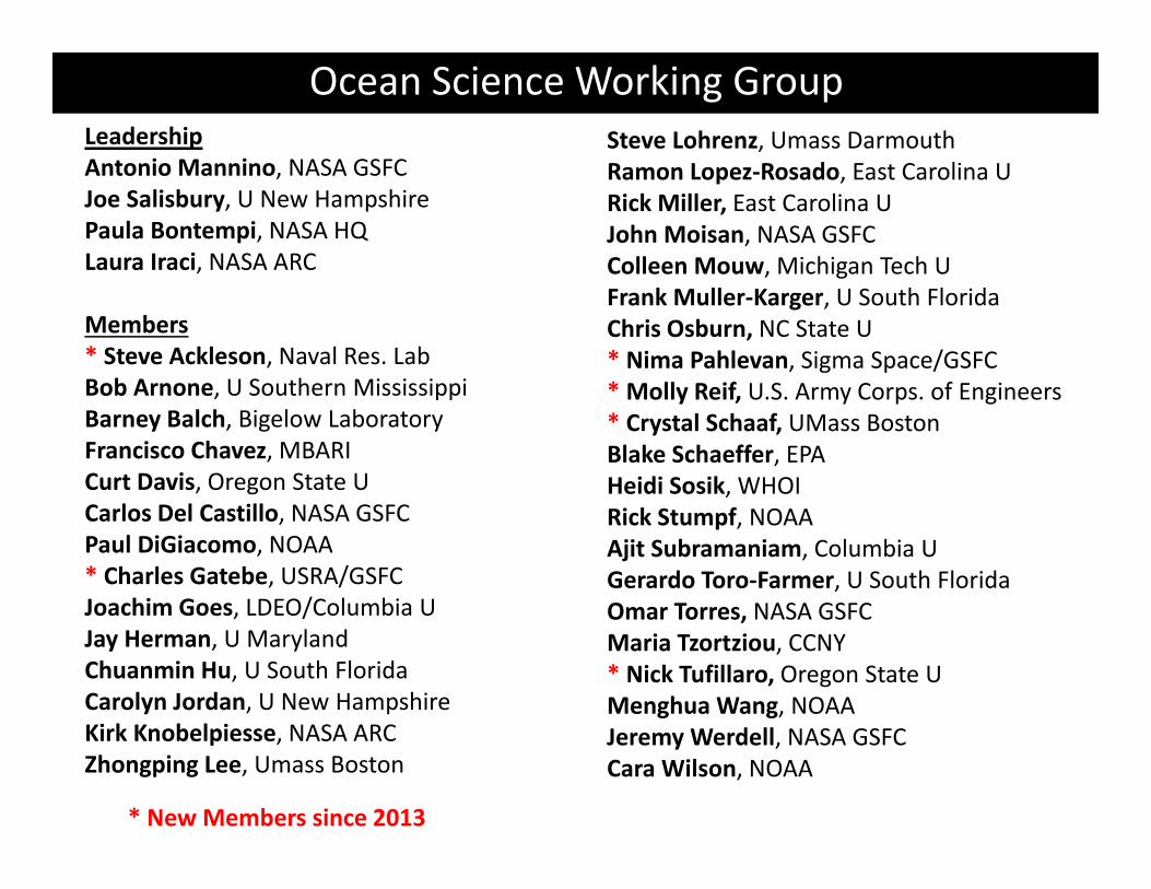
Steve Lohrenz, Umass DarmouthRamon Lopez‐Rosado, East Carolina U Rick Miller, East Carolina UJohn Moisan, NASA GSFCColleen Mouw, Michigan Tech U Frank Muller‐Karger, U South Florida Chris Osburn, NC State U* Nima Pahlevan, Sigma Space/GSFC * Molly Reif, U.S. Army Corps. of Engineers* Crystal Schaaf, UMass BostonBlake Schaeffer, EPA Heidi Sosik, WHOI Rick Stumpf, NOAA Ajit Subramaniam, Columbia UGerardo Toro‐Farmer, U South Florida Omar Torres, NASA GSFCMaria Tzortziou, CCNY * Nick Tufillaro, Oregon State U Menghua Wang, NOAA Jeremy Werdell, NASA GSFCCara Wilson, NOAA

Ocean Science Working GroupLeadershipAntonio Mannino, NASA GSFCJoe Salisbury, U New HampshirePaula Bontempi, NASA HQLaura Iraci, NASA ARC

Members* Steve Ackleson, Naval Res. Lab Bob Arnone, U Southern Mississippi Barney Balch, Bigelow LaboratoryFrancisco Chavez, MBARICurt Davis, Oregon State U Carlos Del Castillo, NASA GSFCPaul DiGiacomo, NOAA * Charles Gatebe, USRA/GSFC Joachim Goes, LDEO/Columbia U Jay Herman, U Maryland Chuanmin Hu, U South Florida Carolyn Jordan, U New Hampshire Kirk Knobelpiesse, NASA ARCZhongping Lee, Umass Boston

* New Members since 2013

ocean color science working group highlights - … geo‐cape workshop aug. 31‐sept. 2, 2015 •...

Documents