obtaining thermodynamic properties and fluid phase...

17

Obtaining Thermodynamic Properties and Fluid Phase Equilibria without

Experimental Measurements

Lin, Shiang-Tai and Hsieh, Chieh-Ming Department of Chemical Engineering, National Taiwan University

Taiwan

1. Introduction

The knowledge of thermodynamic properties and phase equilibria of pure and mixture fluids is crucial for the design, development and optimization of chemical, biochemical, and environmental engineering (Sandler, 2006). Conventional thermodynamic models, containing empirical or semi-empirical parameters, are very useful for the correlation of experimental data and have limited predictive capability for conditions beyond the experimental measurements. While a large amount of thermodynamic experiments have been conducted over the past decades, it has been estimated that about 2000 new chemicals are being synthesized everyday (Campbell, 2008). It would be a daunting and impractical task attempting to obtain the thermodynamic properties of these new chemicals and their mixtures with existing chemicals from experiment. Experimental determination of thermodynamic properties can also be quite challenging because of the toxic nature of some chemicals and the conditions of interest may reach the detection limit of modern apparatus (low vapor pressure, infinite dilution, etc.). It is therefore highly desirable to have a reliable means to estimate these important data prior to measurements, or even before the synthesis of the chemicals. In this chapter, we illustrate how the thermodynamic properties and phase behavior of fluids can be obtained from the combination of advances in computational chemistry and the theories of statistical and classical thermodynamics. Instead of regression to experimental data, the model parameters in an equation of state, such as the Peng-Robinson equation of state (Peng & Robinson, 1976), can be determined from the results of first principle solvation calculations. The consequence is a completely predictive approach for almost any thermodynamic properties of all types of fluids (pure and mixture) at all conditions (above and below the critical point) without the need of any experimental data. We show that this is a practical approach for the prediction of pure fluid properties (Hsieh & Lin, 2008) such as the vapor pressure, liquid density, the critical temperature and pressure, as well as the vapor-liquid (Hsieh & Lin, 2009b), liquid-liquid (Hsieh & Lin, 2010), and solid-liquid phase equilibria of mixture fluids. This method also allows for accurate predictions of the distribution of a trace amount of pollutant between two partially miscible liquids, such as the octanol-water partition coefficient (Hsieh & Lin, 2009a). Conventionally, models were developed for a certain specific property of interest.

www.intechopen.com

Application of Thermodynamics to Biological and Materials Science

460

For example, a model that can be used for the vapor pressure cannot be used for the Henry’s law constant, and vice versa. The method we have developed is general and can be used to determine all aspects of properties of a chemical under any conditions. Furthermore, the method developed here does not suffer from the problem of missing parameters that is commonly seen in the group contribution method and applicable to many more problems than the quantitative structure-activity relationship for property estimation. The accuracy of property predictions from our method is comparable or superior to most existing methods.

2. Equations of state

A thermodynamic equation of state is the mathematical equation that describes the interrelationship between thermodynamic variables (Prausnitz et al., 2004). One of such equations is the pressure(P)-volume(V)-temperature(T)-composition(x) equation of state, which is commonly expressed as

z=f(T,V,x) (1)

where z=PV/RT is the compressibility factor of a fluid. (Note that V=V/N is the molar volume, x=(x1,x2,…, xc) denotes the mole fractions of all the components.) In the case of an ideal gas, the function f(T,V,x) is unity regardless of temperature and concentration of the fluid, i.e., z=1. In general, the compressibility factor of a fluid is a function of its temperature, pressure, and composition. For example, a widely used Peng-Robinson equation of state (Peng & Robinson, 1976) describes the compressibility of a fluid as follows

( , )

( , , )( ) ( ) ( )

V a T x Vz T V x

V b x RT V V b b V b= −− + + − (2)

where a(T, x) and b(x) are the energy and volume parameters, respectively. (For a review of other types of equations of state, please refer to (Kontogeorgis & Folas, 2010, Poling et al., 2001, Prausnitz et al., 2004, Sandler, 2006)). Conventionally, the two interaction parameters in the Peng-Robinson equation of state are determined from the critical properties of the fluid. For example, for pure fluids

22 2

,

, ,( ) 0.45724 1 1c i

i ic i c i

R T Ta T

P Tκ⎡ ⎤⎛ ⎞⎢ ⎥⎜ ⎟= + −⎜ ⎟⎢ ⎥⎝ ⎠⎣ ⎦

(3)

and

,

,0.07780 c i

ic i

RTb

P= (4)

where Tc,i, Pc,i are the critical temperature and pressure of substance i, and the parameter k is

20.37464 1.54226 0.26992i i iκ ω ω= + − (5)

with ωi being the acentric factor. For mixtures, it is necessary to determine the composition dependence of the interaction parameters a(T, x) and b(x). One common approach is to

www.intechopen.com

Obtaining Thermodynamic Properties and Fluid Phase Equilibria without Experimental Measurements

461

assume the a quadratic composition dependence, such as in the van der Waals one-fluid mixing rule

1 1

( , )c c

i j iji j

a T x x x a= =

= ∑∑ (6)

and

1 1

( )c c

i j iji j

b x x x b= =

= ∑∑ (7)

where aij and bij are determined from the combining rule

( ) ( )(1 )

( ) / 2ij i j ij

ij i j

a a T a T k

b b b

= −= + (8)

with kij being the binary interaction parameter whose value must be determined from fitting to experimental data. There are other more advanced mixing rules, where a(T, x) and b(x) are obtained by matching the equation of state to other physical properties (such as the excess Gibbs free energy). Interested readers are refer to the book (Kontogeorgis & Folas, 2010) for further details.

2.1 Thermodynamic properties and phase equilibria from an equation of state

Equations of state are widely adopted in process simulators, such as the AspenPlus (AspenTech, 2007), for chemical processes. All thermodynamic properties of a fluid can be obtained from an accurate equation of state, together with the ideal gas heat capacities of all the fluid components. For example, the Gibbs free energy of a mixture fluid at certain temperature and pressure can be calculated from

,

,( , , ) ( , , ) ( 1) ln

T VIGM

T V

RTG T P x G T P x RT z RT z P dV

V=∞⎡ ⎤= + − − + −⎢ ⎥⎣ ⎦∫ (9)

where GIGM(T,P,x) is the Gibbs free energy of an ideal gas mixture at the same condition as the fluid of interest and can be determined from

1

( , , ) ( , ) lnc

IGM IGi ii

i

G T P x x G T P RT x=

= +∑ (10)

where GiIG(T,P) is the Gibbs free energy of pure species i in an ideal gas state at T and P. The ideal gas contribution can be obtained with high accuracy with modern computational chemistry (Foresman & Frisch, 1996, Ochterski, 2000). As seen in equation 9, the property deviation from ideal gas contributions can be obtained from an equation of state. When the Peng-Robinson equation of state (eqn. 2) is used, equation 9 becomes

(1 2 )

( , , ) ( , , ) ( 1) ln( ) ln2 2 (1 2 )

IGM A z BG T P x G T P x RT z RT z B

B z B

⎡ ⎤+ += + − − − − ⎢ ⎥+ −⎢ ⎥⎣ ⎦ (11)

www.intechopen.com


462

where A=Pa/(RT)2 and B=Pb/RT are dimension less quantities. Other thermodynamic properties, such as the internal energy, enthalpy, entropy, Helmholtz free energy, ect., can be determined in a similar fashion (Sandler, 2006). When there are multiple phases coexisting in a system, the equilibrium composition of each phase can be determined from the equivalence of fugacity of each chemical in all phases

( , , ) ( , , ) ( , , )I II IIII II IIIi i if T P x f T P x f T P x= = =A (12)

where the superscripts I, II, III, etc indicate the phase of interest. Therefore, determination of fugacity is the key in phase equilibrium calculations. This quantity can be calculated if an equation of state of the fluid is known

,

,, ,

( , , ) 1ln ln

j i

T Vi

T Vi i T V N

f T P x RT Pz N dV

x P RT V N ≠=∞

⎡ ⎤⎛ ⎞∂⎢ ⎥= − + − ⎜ ⎟⎢ ⎥∂⎝ ⎠⎣ ⎦∫ (13)

and when the Peng-Robinson equation of state and van der Waals mixing rule is assumed for the fluid, equation 13 becomes

1

( , , )ln ( 1) ln( )

2(1 2 )

ln2 2 (1 2 )

i i

i

c

i ijj i

f T P x Bz z B

x P B

x ABA z B

A BB z B

=

= − − −⎡ ⎤⎢ ⎥ ⎡ ⎤+ +⎢ ⎥− − ⎢ ⎥⎢ ⎥ + −⎢ ⎥⎣ ⎦⎢ ⎥⎢ ⎥⎣ ⎦

∑ (14)

where Aij=Paij/(RT)2. From the above examples, it is clear that an accurate equation of state is very important for obtaining the thermodynamic properties and phase behaviours of a fluid. However, in conventional approaches the necessary parameters in an equation of state (a(T, x) and b(x)) require input of several experimental data, including the critical properties and acentric factor of pure substances, and some mixture data (such as the vapor-liquid equilibrium data) for determining kij. The need of experimental input severely restricts the application of an equation of state. For example, the critical properties of high molecular weight compounds (e.g., polymers, proteins, heavy organics, etc.) are not experimentally available as they would decompose before reaching the critical point. More importantly, the need for binary interaction parameter kij posses issues for processes involving new chemicals (e.g., drug discovery) where scarce or even no data is available. We will illustrate how the use of computational chemistry, in particular, quantum mechanical solvation calculations, to resolve these difficulties.

2.2 Solvation properties from an equation of state

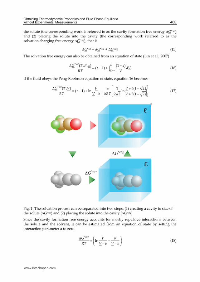
The solvation free energy ∆G*sol, as defined by Ben-Naim (Ben-Naim, 1987), is the work needed for transferring of a molecule (solute) from an ideal gas phase to a solution (solvent) under constant temperature T and pressure P. Such a free energy is commonly computed from a hypothetical two-step process, as illustrated in Figure 1: (1) creating a cavity to size of

www.intechopen.com


463

the solute (the corresponding work is referred to as the cavity formation free energy ∆G*cav) and (2) placing the solute into the cavity (the corresponding work referred to as the solvation charging free energy ∆G*chg), that is

ΔG*sol = ΔG*cav + ΔG*chg (15)

The solvation free energy can also be obtained from an equation of state (Lin et al., 2007)

* ( , , ) (1 )

( 1)sol

V

V

G T P x zz dV

RT V=∞Δ −= − + ∫ (16)

If the fluid obeys the Peng-Robinson equation of state, equation 16 becomes

* ( , ) 1 (1 2 )

( 1) ln ln2 2 (1 2)

solG T V V a V bz

RT V b bRT V b

⎡ ⎤Δ + −= − + + ⎢ ⎥− + +⎢ ⎥⎣ ⎦ (17)

∆G*cav

∆G*chg

ε

ε

Fig. 1. The solvation process can be separated into two steps: (1) creating a cavity to size of the solute (∆G*cav) and (2) placing the solute into the cavity (∆G*chg)

Since the cavity formation free energy accounts for mostly repulsive interactions between the solute and the solvent, it can be estimated from an equation of state by setting the interaction parameter a to zero.

*

lncavG V b

RT V b V b

⎛ ⎞Δ = +⎜ ⎟− −⎝ ⎠ (18)

www.intechopen.com


464

Therefore, the changing free energy must be

*

2 2

1 (1 2 )ln

2 2 (1 2) 2

chgG a V b bV aC

RT bRT bRTV b V bV b

⎡ ⎤Δ + −= − =⎢ ⎥+ + + −⎢ ⎥⎣ ⎦ (19)

where the variable C represents the terms in the square brackets, and its value depends on the density of the fluid. Equations 19 provides a new way of obtaining the equation of state parameters from solvation calculations

*( )( , ) ( , , )

( )chgb x

a T x G T V xC V

= Δ (20)

The choice of density for evaluation of C must be consistent with that using in the solvation calculations. Our previous studies (Hsieh & Lin, 2009b) showed that C=-0.623 is a good choice for the Peng-Robinson equation of state. The size parameter b(x) can be approximated in a way similar to the van der Waals mixing rule

( ) i ii

b x x b= ∑ (21)

and the size of pure component bi can be approximated using the volume of the cavity (see Fig. 1) used in solvation calculations. Therefore, equations 20 and 21 provide a new route to the temperature and composition dependence of parameters in the Peng-Robinson equation of state completely from solvation properties.

2.3 Equation of state parameters from first principle solvation calculations

A solvation model is necessary for the charging free energy in equations 20. Here we choose to use the method proposed by Lin et al. (Lin et al., 2007), in which the charging free energy is the summation of contributions from all components in the mixture

* */

1( , )

cchg chg

i ji

G G T x=

Δ = Δ∑ (22)

and the molecular charging free energy is the sum of four contributions (Lin et al., 2004),

* * * * */ /( , ) ( ) ( , )chg is cc dsp res

i j i i i i jG T x G G G T G T xΔ = Δ + Δ + Δ + Δ (23)

where the superscripts is, cc, res, and dsp denote ideal solvation, charge-averaging correction, restoring, and dispersion contribution to the solvation charging free energy. In this solvation model, the solute molecule is first dissolved into a fluid of infinite dielectric constant (or a conductor), where the solute molecule is perfectly screened. The first three terms on the right and side of equation 23 account for the free energy change in this process. Finally, the chemical nature of the solvent is restored (reducing the dielectric constant from infinity to its physical value at temperature T), and the corresponding free energy is referred to as the restoring free energy (the last term of eqn. 23). The ideal solvation term is the difference in energy when the solute is in the ideal gas and in the conductor state

www.intechopen.com


465

Water

1-butanol

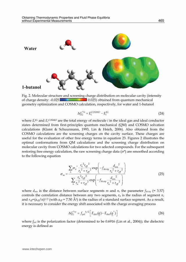
Fig. 2. Molecular structure and screening charge distribution on molecular cavity (intensity of charge density: -0.025 0.025) obtained from quantum mechanical geometry optimization and COSMO calculation, respectively, for water and 1-butanol

*is COSMO IGi iiG E EΔ = − (24)

where EiIG and EiCOSMO are the total energy of molecule i in the ideal gas and ideal conductor states determined from first-principles quantum mechanical (QM) and COSMO solvation calculations (Klamt & Schuurmann, 1993, Lin & Hsieh, 2006). Also obtained from the COSMO calculations are the screening charges on the cavity surface. These charges are useful for the evaluation of other free energy terms in equation 23. Figures 2 illustrates the optimal conformations from QM calculations and the screening charge distribution on molecular cavity from COSMO calculations for two selected compounds. For the subsequent restoring free energy calculation, the raw screening charge data (σ*) are smoothed according to the following equation

2 2 2*

2 2 2 2

2 2 2

2 2 2 2

exp

exp

n eff mnn decay

n n eff n eff

m

n eff mndecay

n n eff n eff

r r df

r r r r

r r df

r r r r

σσ

⎛ ⎞⎜ ⎟−⎜ ⎟+ +⎝ ⎠= ⎛ ⎞⎜ ⎟−⎜ ⎟+ +⎝ ⎠

∑∑

(25)

where dmn is the distance between surface segments m and n, the parameter fdecay (= 3.57) controls the correlation distance between any two segments, rn is the radius of segment n, and reff=(aeff/π)1/2 (with aeff = 7.50 Å2) is the radius of a standard surface segment. As a result, it is necessary to consider the energy shift associated with the charge averaging process

* *1/2 ( ) ( )ccpol diel dieliG f E q E q⎡ ⎤Δ = −⎣ ⎦ (26)

where fpol is the polarization factor (determined to be 0.6916 (Lin et al., 2004)); the dielectric energy is defined as

www.intechopen.com


466

1

( )2dielE q qν νν

φ= ∑ (27)

here qv is the screening charge at some position v on the cavity surface and φv is the electrostatic potential due to the solute at position v. Both qv and φv are obtained from the COSMO solvation calculation. The screening charges distributed on the cavity surface are quantified by the sigma-profile, p(σ), based on the fraction of surfaces possessing a certain charge density value σ

( )

( ) ii

i

Ap

A

σσ = (28)

where Ai is the total surface area of species i. To better account for the interactions between species that may form a hydrogen bond, the surfaces may be further categorized to four types: surfaces that do not involve in a hydrogen bond Ainhb, surfaces from hydroxyl groups Aihydro, surfaces from amino groups of primary and secondary amines Aiamino, and all other surfaces that may be involved in a hydrogen bond Aiother, such as -NO2. Therefore, the sigma-profile is refined as

( ) ( ) ( ) ( )

( )

( ) ( ) ( ) ( )

hydronhb amino otheri i ii

i

hydronhb amino other

A A A Ap

A

p p p p

σ σ σ σσσ σ σ σ

+ + +== + + +

(29)

Figure 3 illustrates the sigma-profile of a few common chemicals. The sigma-profile is in fact the probability distribution of screening charges. In a mixture, such probability distribution can be calculated as the mole-fraction average of contributions from the pure components

( )

( )i i i

iS

i ii

x A p

px A

σσ = ∑

∑ (30)

The sigma profile reflects the electronic nature of a chemical species and is unique to each chemical. Therefore, it was used to determine the restoring free energy (Lin & Sandler, 2002, Hsieh & Lin, 2010)

nhb, hydro,* amino, other/ ( )ln ( )

m

resi j s s s si

i m j meff s

G Ap

RT a σσ σ⎡ ⎤Δ = Γ⎢ ⎥⎢ ⎥⎣ ⎦∑ ∑ (31)

where Γ is the segment activity coefficient

( ) ( ) ( ) nhb, hydro,amino, other ,

ln ln exp ln ( )n

t sm nt t s s s s

j m j n j ns

Wp

RTσσ σσ σ σ

⎧ ⎫⎡ ⎤−Δ⎪ ⎪⎢ ⎥Γ = − + Γ⎨ ⎬⎢ ⎥⎪ ⎪⎣ ⎦⎩ ⎭∑ ∑ (32)

The segment interaction energy ∆W is determined by considering the electrostatic and hydrogen bonding interactions between two contacting surfaces

www.intechopen.com


467

Fig. 3. The sigma profiles for four representative compounds: acrylonitrile (solid line), monoethanolamine (long dashed line), isobutyric acid (short dashed line), and water (dashed-dotted line). Ai is the molecular surface area of species i.

( )3/22 2

0

0.3( , ) ( , )( )

2efft s t s t s t s

m n pol m n hb m n m n

aW f cσ σ σ σ σ σ σ σεΔ = + − − (33)

where ε0 is the permittivity of vacuum; coefficient ( , )t shb m nc σ σ is temperature-independent

and its value is determined according to the type of the interacting segments

HH

AA

OO

hb HA

HO

if s t hydro and 0

if s t amino and 0

if s t other and 0

( , ) if s hydro, t amino, and 0

if s hydro, t other, and

t sm n

t sm n

t sm n

t s t sm n m n

m

c

c

c

c c

c

σ σσ σσ σ

σ σ σ σσ

= = ⋅ <= = ⋅ <= = ⋅ <

= = = ⋅ <= =

AO

0

if s amino, t other, and 00 otherwise

t sn

t sm nc

σσ σ

⎧⎪⎪⎪⎪⎪⎨⎪ ⋅ <⎪⎪ = = ⋅ <⎪⎪⎩

(34)

www.intechopen.com


468

The six parameters (cHH, cAA, cOO, cHA, cHO, and cAO) in equation 34 are universal constants. Their values have been determined using experimental vapor pressure data of selected pure substances and selected liquid-liquid equilibria, and do not need to be changed.

Universal Parameters

Parameter Value Parameter Value

CPR -0.623 cHH (kcal/mol)(Å4/e2) 1757.9468

aeff (Å2) 7.50 cAA (kcal/mol)(Å4/e2) 1121.4047

fpol 0.6916 cOO (kcal/mol)(Å4/e2) 1757.9468

fdecay 3.57 cHA (kcal/mol)(Å4/e2) 2462.3206

Adsp,HB (J/mol/K/Å2) -465876.8150 cHO (kcal/mol)(Å4/e2) 933.4108

Bdsp,HB (J/mol/Å2) -429.5556 cAO (kcal/mol)(Å4/e2) 2057.9712

Cdsp,HB (J/mol/K2/Å2) -141.8436

Adsp,RING (J/mol/K/Å2) -0.9181

Bdsp,RING (J/mol/Å2) -365.0667

Atom Specific Parameters

atom type radius Ri (Å) Adsp,i (J/mol/K/Å2) Bdsp,i (J/mol/Å 2)

H 1.30 0.1694 -191.4602

C 2.00 0.1694 -191.4602

N 1.83 0.4045 -207.9411

O 1.72 0.2701 -178.0767

F 1.72 0.1806 -125.7842

Cl 2.05 0.1566 -201.7754

Table 1. Parameters and their values in the PR+COSMOSAC EOS

The dispersion solvation free energy is considered to be proportional to the exposed surface area of the atom comprising the molecule (Cramer & Truhlar, 1991, Cramer & Truhlar, 2008, Klamt, 1995, Klamt et al., 1998, Lin et al., 2004, Lin & Sandler, 2002, Still et al., 1990, Tomasi & Persico, 1994). Here we propose a slightly modified form to better describe ring containing and hydrogen bonding chemicals.

* * *, ,( ) ( ) ( ) ( )dsp dsp dsp

j dsp j dsp ji HB RINGj

G T s A T B G T G TΔ = + + +∑ (35)

where sj is the total exposed surface area of atom type j, Adsp,j and Bdsp,j are the dispersion parameters of atom type j, and *dsp

HBG and *dspRINGG are the empirical corrections for hydrogen-

bonding and cyclic (or aromatic) containing molecules. The expressions of these two terms are

( ),*

, ,

1( )

1 exp /

dsp HBdspHB

HBH dsp HB dsp HB

AG T

N T B C

⎧ ⎫⎪ ⎪= ⎨ ⎬⎡ ⎤+ − −⎪ ⎪⎣ ⎦⎩ ⎭ (36)

www.intechopen.com


469

and

*, ,( ) ( )dsp

AR dsp RING dsp RINGRINGG T N A B= + (36)

where NHBH and NAR are the number of hydrogen-bonding donors (the hydrogen atoms connecting to either nitrogen, oxygen, or fluorine atom) and the number of atoms involved in any ring-structure, respectively. All the parameters in the proposed model have been determined by regression to experimental vapor pressure of selected compounds or experimental data of binary liquid-liquid equilibrium. They are summarized in Table 1. Once the solvation charging free energy at some given temperature and solution composition is determined from equations 22 to 36, the energetic parameter a(T,x) in the PR EOS can be calculated from equation 20. This approach is referred to as PR+COSMOSAC hereafter. It is useful to note that the fugacity coefficient can be determined analytically from the PR+COSMOSAC equation of state as follows (Hsieh and Lin, 2010)

*/( , , )

ln ln 1 lnchg

i Si i

i

Gf T P x PbPbz

x P RT zRT zRT Pb

Δ ⎛ ⎞= − − + −⎜ ⎟ −⎝ ⎠ (37)

3. Prediction of thermodynamic properties and phase equilibria

The PR+COSMOSAC equation of state contains 15 universal constants and 3 element specific coefficients, as shown in Table 1. This set of parameters is all that is needed to determine all kinds of thermodynamic properties and phase equilibria of any system. In the following, we illustrate some of the properties predicted from PR+COSMOSAC. The procedure of calculation of thermodynamic properties can be found in most text books such as (Prausnitz et al., 2004, Sandler, 2006).

3.1 Thermodynamic properties of pure fluids

As a first example, the PR+COSMOSAC is used to predict the vapor-liquid coexisting curve of pure fluids all the way to the critical point. Figure 4 shows the pressure-volume and pressure-temperature diagrams for two chemical species having very different critical pressures: 1,3-propylene glycol (high Pc= 9.5 MPa), cyclooctane (low Pc= 3.57 MPa). The solid and grey lines are the results from the proposed method and the original PR EOS. The temperature dependence of the vapor pressure is well described for these compounds (Fig. 4a). The deviations of liquid molar volume and the gas molar volume from proposed model are similar to those from original PR EOS (Fig. 4b). Although the agreement is not perfect, the present model shows how effectively a theoretically-based statistical mechanical model can describe the temperature-dependent parameter a(T) in the PR EOS. Another important application of the PR+COSMOSAC equation of state is the prediction of the normal boiling point of environmentally important chemicals. The normal boiling point is an indication of the volatility of a chemical, and therefore is an important quantity needed in many chemical, biochemical, and environmental studies. These hazardous chemicals are often complex in their chemical structure and have a low vapor pressure at ambient conditions, making direct experimental measurement quite challenging. Figure 5 shows the comparison of predicted and measured normal boiling point of 63 environmentally significant compounds (including chemical such as dichloro acetic aced, D-limonene, isoprene, perchlorocyclopentadiene, acridine, 2-chlorobiphenyl (PCB-1), etc.). As can be seen

www.intechopen.com


470

that there is a very good agreement between the predicted and experimental values (most of the data points lay on the diagonal line). The overall average absolute error from the PR+COSMOSAC model is 3.8% for the normal boiling temperature.

Fig. 4. The pressure-temperature (a) and pressure-volume (b) diagrams from the original PR EOS (gray lines) and the PR+COSMOSAC with (solid lines) for cyclooctane and 1,3-propylene glycol. The experimental data (DIPPR, 2008) are shown in squares and circles for the two compounds, respectively

Fig. 5. Comparison of normal boiling temperatures for environmentally important chemicals from experiments and predictions from PR+COSMOSAC equation of state

Unlike the conventional approach where the critical properties are used to determine the interaction parameters in the Peng-Robinson equation of state (eqn. 3 to 5), the PR+COSMOSAC determines these parameters from solvation calculations (eqn. 20 and 21). Therefore, critical properties of pure fluids can be now calculated. Figure 6 illustrates the comparison of experimental and predicted critical properties for compounds whose experimental critical properties are available in the DIPPR database (346, 431, and 270 compounds in critical pressure Pc, critical temperature Tc, and critical volume Vc, respectively). The critical volume is estimated from the volume of solvation cavity in COSMO calculation. The predicted Vc are in good agreement with experiment for small compounds (e.g., Vc < 0.6 m3/kmol). It has been observed previously that the critical volume is highly correlated with

www.intechopen.com


471

the molecular size (Kontogeorgis et al., 1997). We also found a good linear correlation between the value of parameter b determined from the solvation cavity and that from Tc and Pc in the PR EOS. These results show that the atomic radii (Table 1) used in establishing the solvation cavity are adequate for describing the volume parameter b. The larger deviations (underestimation) found for larger compounds could be attributed to the ignorance of conformation flexibility in current calculations (e.g., long chain alkanes are modeled as linear but they could be folded in reality) and/or the ignorance of molecular shape effects in the PR EOS (the cavity term in PR EOS is valid for spherical molecules (Lin, 2006)).

Fig. 6. Comparison of critical properties from experiments and predictions. The marked species are (A) carbon monoxide, (B) methacrylic acid, (C) hydrogen fluoride, (D) hydrogen cyanide, (E) acetonitrile, (F) nitrogen tetroxide, (G) ammonia, (H) hydrazine, (I) water, (J) carbon monoxide, and (K) propionitrile

The deviations in Tc are less than 120 K, except for carbon monoxide and methacrylic acid, marked by A and B, respectively, in Figure 6. Once Vc and Tc are known, the critical pressure can be calculated from Pc = zcRTc/Vc. While the PR EOS has a fixed value of critical compressibility factor (zc = 0.307) for all compounds, experimental values of zc range from 0.2 to 0.3 for most chemicals (DIPPR, 2008, Poling et al., 2001). Therefore, we have rescaled the calculated Pc by 0.26/0.307 in Figure 6 for better accuracy. [Note that the use of zc = 0.26 is recommended for calculation of Pc only and is not used in any other property calculations

www.intechopen.com


472

(e.g. the vapor pressure).] The poorly predicted Pc found in Figure 6 (marked as C to K) are caused either by the constant critical compressibility factor (zc = PcVc/RTc) in the PR EOS or the error in the predicted Tc. For example, hydrogen fluoride (marked C) has zc = 0.117 and ammonia (marked G) has zc = 0.242 but has a deviation of 73 K in predicted Tc.

3.2 Vapor-liquid, liquid-liquid, and vapor-liquid-liquid equilibria

Figure 7 shows the P-x-y diagram for morpholine/n-octane binary mixtures at two temperatures, 330 K and 340 K. While the predictions from PR+COSMOSAC (dashed lines) are in reasonable agreement with experiments (open circles), the predicted total pressure are slightly too high in the low morpholine concentration regime. This is a result of the over prediction of the vapor pressure of n-octane from PR+COSMOSAC. The predictions can be further improved if some experimental data is used to correct for the inaccuracy found for the vapor pressure.

Fig. 7. P-x-y phase diagram of vapor-liquid equilibrium for morpholine (1) + n-octane (2) (a type II system). The dashed, solid, and gray lines are predicted results from PR+COSMOSAC, PR+COSMOSAC+TcPcω, and PR+COSMOSAC+Pvap, respectively. The experimental data, taken from (Wu et al., 1991), are shown as open circles

* * */ / ,Corr[eqn. 23] ( )chg chg chg

i S i S iG G G TΔ = Δ + Δ (38)

One possible correction is to adjust *,Corr( )chg

iG TΔ so that correct vapor pressure of species i is obtained at temperature T. This approach, denoted as PR+COSMOSAC+Pvap, ensures correct pressures in the VLE phase diagram in the pure fluid limits. Figure 7 also shows the predictions from PR+COSMOSAC+Pvap (gray). It can be seen that the predictions are significantly improved. One limitation of PR+COSMOSAC+Pvap is that it is not applicable for problems at temperatures above the critical point of its component (e.g. determination the solubility of a gas in liquid). Figure 8 shows the vapor-liquid equilibrium diagram of 2-propanol/water binary mixture at five temperatures. While the PR+COSMOSAC model captures the general phase behavior of this mixture, it is quantitatively inaccurate due to the under prediction of

www.intechopen.com


473

the vapor pressure of water. At temperatures above the critical point of 2-propanol (~508 K) the correction of eqn. 38 cannot be applied. Another possible correction method is to use the critical properties (Tc and Pc) and acentric factor (ω),

* *,Corr /( ) [eqn. 23]chg chg i

i i ii

a CG T G

bΔ = −Δ + (39)

Equation 39 ensures the same vapor pressure as that from the Peng-Robinson EOS is obtained. This approach is denoted as PR+COSMOSAC+TcPcω. Using this correction, the vapor pressure of water is correctly obtained and the phase diagram of 2-propanol/water can be accurately predicted (see the solid curves in Figure 8).

Fig. 8. P-x-y phase diagram of vapor-liquid equilibrium for 2-propanol (1) + water (2) (a type III system). The lines have the same meanings as in Figure 7. The experimental data, taken from Barr-David and Dodge (Barr-David & Dodge, 1959) and Sada and Morisue (Sada & Morisue, 1975), are shown as open symbols

Fig. 9. Comparison of predicted (dashed lines) and experimental (open circles)(Sørensen & Arlt, 1979) liquid-liquid equilibrium for furfural (1) + 2,2,5-trimethylhexane (2) (left panel) and 2,4-pentanedione (1) + water (2) (right panel)

www.intechopen.com


474

Figure 9 illustrates two examples of liquid-liquid equilibrium predictions from PR+COSMOSAC. In the mixture of furfural/2,2,5-trimethylhexane, no hydrogen bond is present. It can be seen that the PR+COSMOSAC describes the miscibility gap accurately all the way to the upper critical solution temperature. In the second example of 2,4-pentanedione/water, hydrogen bonds may be present between like species (water) and unlike species (water-2,4-pentanedione). The predictions from PR+COSMOSAC are again in quantitative agreement with the experiments. As one last example of fluid phase equilibria predictions from PR+COSMOSAC, Figure 10 shows the vapor-liquid-liquid equilibrium of water/ethyl acetate at one atmospheric pressure. The PR+COSMOSAC model, without use of any experimental data, is able to capture the general features of VLLE. Because of the under estimation of the vapor pressure of water, the predicted normal boiling point is too high, leading to an over estimation of the three phase coexisting temperature. However, when the critical properties are introduced, i.e., the PR+COSMOSAC+TcPcω, the predictions are in excellent agreement with experiment both in the VLE, LLE, and the coexisting temperature. In general, accurate VLLE predictions can be achieved if a model is accurate on both VLE and LLE. Furthermore, good description on LLE helps in getting better liquid phase compositions; whereas good description on VLE helps in getting better equilibrium temperature and gas phase composition. From the previous examples, the PR+COSMOSAC model usually provides good descriptions for the liquid phase non-ideality; however, its performance in the phase vapor is less accurate, mainly because of its deficiency in describing the vapor pressure of pure fluids. The PR+COSMOSAC+TcPcω model thus serves as an effective compromise for both vapor and liquid phase equilibrium predictions.

Fig. 10. Comparison of VLLE from experiments and predictions for water(1) + ethyl acetate(2). The open squares and triangles are experimental VLE and LLE(Gmehling et al., 1977, Sørensen & Arlt, 1979). The dashed lines and solid lines are results from PR+COSMOSAC and PR+COSMOSAC+TcPc ω, respectively

www.intechopen.com


475

3.3 Solubility of drugs

The knowledge of drug solubility is important in the design of drug manufacturing processes. Solvent screening is often necessary to identify optimal operating conditions for synthesis, reaction, and purification (Constable et al., 2007, Modarresi et al., 2008). However, experimental approaches are both time-consuming and costly since there essentially are an infinite number of combinations of possible solvent mixtures. Furthermore, as the drug discovery techniques continue to improve, the number of potential drug candidates increases significantly. It is impractical to measure the solubility data for all drug candidates in all possible solvent combinations. Thus, a predictive thermodynamic model can help to overcome this obstacle. Numerous thermodynamic methods are used to predict the solubility of organic compounds in the literature (Chen & Crafts, 2006, Chen et al., 2008, Klamt et al., 2002, Mullins et al., 2008, Shu & Lin, 2010, Tung et al., 2008). Here, we illustrate the prediction of drug solubility from PR+COSMOSAC. The solubility of 52 drug compounds [from the smallest iodine (2 atoms) to the largest testosterone (49 atoms)] in 37 different pure solvents are considered. There are a total of 171 drug-solvent pairs for drug solubility in pure solvent and 156 mixture solvent combinations (298 systems), including 3 ternary solvent mixtures (10 systems) and 1 quaternary solvent mixture (1 system). The solubility data cover a wide range of values, from 10-1 to 10-6 (by mole fractions) over a temperature of 273.15 K to 323.15 K. In the calculation of solid solubility, the following relations (derived from considering solid-liquid equilibrium) is used

,

( , , )1 1ln ln

( , )

fus Sii

im i i i

H f T P xx

R T T x f T P

⎛ ⎞Δ= − −⎜ ⎟⎜ ⎟⎝ ⎠ (40)

where Sif is the fugacity of the drug in the solvent, fi is the fugacity of a hypothetical pure

liquidus drug, Tm,i and ∆Hifus are the melting temperature and the enthalpy of fusion at melting temperature of the drug. Experimental (Marrero & Abildskov, 2003, Linstrom & Mallard, 2010) values of Tm,i and ∆Hifus are used, while the PR+COSMOSAC model is used for the fugacities.

Fig. 11. Comparison of solubility (in logarithm) of 52 drugs in 37 pure solvents (362 data points) from experiments and predictions from PR+COSMOSAC

www.intechopen.com


476

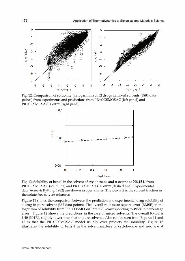
Fig. 12. Comparison of solubility (in logarithm) of 52 drugs in mixed solvents (2894 data points) from experiments and predictions from PR+COSMOSAC (left panel) and PR+COSMOSAC+Gdsporr (right panel)

Fig. 13. Solubility of benzil in the solvent of cyclohexane and n-octane at 298.15 K from PR+COSMOSAC (solid line) and PR+COSMOSAC+Gdsporr (dashed line). Experimental data(Acree & Rytting, 1982) are shown in open circles. The x-axis X is the solvent fraction in the solute free solvent mixtures

Figure 11 shows the comparison between the prediction and experimental drug solubility of a drug in pure solvent (362 data points). The overall root-mean-square error (RMSE) in the logarithm of solubility from PR+COSMOSAC are 1.78 (corresponding to 495% in percentage error). Figure 12 shows the predictions in the case of mixed solvents. The overall RMSE is 1.40 (304%), slightly lower than that in pure solvents. Also can be seen from Figures 11 and 12 is that the PR+COSMOSAC model usually over predicts the solubility. Figure 13 illustrates the solubility of benzyl in the solvent mixture of cyclohexane and n-octane at

www.intechopen.com


477

298.15 K. It can be seen that PR+COSMOSAC captures the concentration dependence of the solubility on the solvent composition (in this case, a nearly linear dependence), however, the predicted solubilities are in general too high. Figure 14 illustrates the solubility of acetanilide in the solvent of water and dioxane. In this case, the solubility can vary by about two hundreds folds (from 0.0011 in pure water to 0.21 in pure dioxane) as the composition of the solvent changes. The PR+COSMOSAC model is able to capture such large variations in solubility due to the change in solvent compositions. The inaccuracy in PR+COSMOSAC can be attributed to its lack of accuracy in describing the drug-solvent interactions. The predictions in mixed solvent can thus be improved if the experimental solubility data of the drug in pure solvents are introduced to correct any error in the PR+COSMOSAC model, i.e.,

* dsp,corr,Corr( )chg

kikik

G T G XΔ = ∑ (41)

where Gikdsp,corr is the dispersion free energy correction coefficient for solute i in solvent k; Xk is the solvent fraction in the solute free solvent mixtures. In the case of a single solvent, the correction term becomes

* dsp,corr,Corr( )chg

ikiG T GΔ = (42)

and the coefficient Gikdsp,corr can be determined from fitting to experimental solubility data of the drug in pure solvent i. This approach is denoted as PR+COSMOSAC+Gdsporr. By using the solubility in pure solvents, the RMSE of the predicted solubility in mixed solvents (see also Figure 12) significantly reduces to 0.65 (or 91%). In Figures 13 and 14, it can be seen that the results from PR+COSMOSAC+Gdsporr (dashed line) are in excellent agreement with the experiments.

Fig. 14. Solubility of acetanilide in the solvent of water and dioxane at 293.15 K from PR+COSMOSAC (solid line) and PR+COSMOSAC+Gdsporr (dashed line). Experimental data(Bustamante et al., 1998) are shown in open circles. The x-axis X is the solvent fraction in the solute free solvent mixtures

www.intechopen.com


478

Figure 15 shows an interesting example where a maximum value of solubility is observed at some intermediate concentrations of the solvent combinations. At 298.15 K, the solubility of sulphisomidine in pure water is 0.0009 and in pure dioxane is 0.0025. The solubility reaches a maximum value of 0.011 when the composition of the water is around 0.54. While the PR+COSMOSAC model (solid line) captures the general solvent composition dependence, the PR+COSMOSAC+Gdsporr model (dashed line) is able to predict the existence of such solubility maximum. Although the accuracy of PR+COSMOSAC in the prediction of drug solubility is still far from accurate, it is capable of providing a priori predictions for compounds without binary interaction parameters and experimental data (the enthalpy of fusion and normal melting temperature of drug are needed). This is very useful for in the early stage of drug discovery and the design of purification processes in the pharmaceutical industry.

Fig. 15. Solubility of sulphisomidine in the solvent of water and dioxane at 298.15 K from PR+COSMOSAC (solid line) and PR+COSMOSAC+Gdsporr (dashed line). Experimental data (Martin et al., 1985) are shown in open circles. The x-axis X is the solvent fraction in the solute free solvent mixtures.

4. Conclusion

The employment of ab initio solvation calculation in determination of cubic equation of state parameters for pure and mixture fluids, denoted as PR+COSMOSAC, has led to a new way for describing fluid phase equilibria without input of experimental data such as critical properties. The solvation calculation presented in this work is capable of capturing the correct composition and temperature dependence of the interaction parameter a(T,x), while the solvation cavity and mole-fraction weighted summation is a good estimate for volume parameter b(x). The PR+COSMOSAC EOS is able to provide reasonable predictions on vapor pressures, liquid densities and critical properties for pure fluids and vapor-liquid equilibrium (VLE), liquid-liquid equilibrium (LLE), vapor-liquid-liquid equilibrium (VLLE) for mixtures, and solid-liquid equilibrium (SLE) with a single model and a single set of parameters. The use of this method in the predictions of solubility of drugs in pure and

www.intechopen.com


479

mixture solvents is also validated. Although not shown here, this method can be used to determine other properties such as heat of vaporization, excess properties, distribution coefficient, infinite dilution activity coefficient, etc. Limited by the accuracy in vapor pressure predictions, this approach presently provides only qualitative results for VLE predictions; however, in the case of mixtures, the predicted accuracy can be improved significantly if the critical properties and acentric factor (PR+COSMOSAC+TcPcω) or the vapor pressure (PR+COSMOSAC+Pvap) are used. The accuracy from PR+COSMOSAC may, in some cases, be inferior to existing group contribution methods, e.g., PSRK or modified UNIFAC. However, because of the proximity effects, methods based on concept of group contributions (e.g., PSRK) may sometimes fail badly if used for compounds that do not belong to the family of compounds used in the parameterization. Furthermore, unlike the group contribution methods (PSRK or modified UNIFAC) whose parameter matrix was optimized against a large set of experimental data, the PR+COSMOSAC contains only a few (about 33) non-species dependent, universal parameters. There is no issue of missing parameters if a new chemical species is involved. The computation-demanding QM calculations have to be done only once for each chemical species and can be stored in a database. Once the database is established (e.g. the VT COSMO database (Mullins et al., 2008)), the time need for phase equilibrium calculations using PR+COSMOSAC is similar to that using group contribution methods on a modern personal computer. We consider the PR+COSMOSAC as an ideal complementary method when the existing models are not applicable or no experimental data are available.

5. References

Acree, W.E. & Rytting, J.H. (1982). Solubility in binary solvent systems. 1. Specific versus nonspecific interactions, Journal of Pharmaceutical Sciences, 71, 2, pp. 201-205,0022-3549.

Aspentech (2007), Aspen Plus Unit Operation Models, Aspen Technology Inc: Burlington, MA Barr-David, F. & Dodge, B.F. (1959). Vapor-Liquid Equilibrium at High Pressures. The

Systems Ethanol-Water and 2-Propanol-Water., J Chem Eng Data, 4, 2, pp. 107 - 121 Ben-Naim, A. (1987). Solvation Thermodynamics, Plenum Press, New York. Bustamante, P.; Romero, S.; Pena, A.; Escalera, B. & Reillo, A. (1998). Enthalpy-entropy

compensation for the solubility of drugs in solvent mixtures: Paracetamol, acetanilide, and nalidixic acid in dioxane-water, Journal of Pharmaceutical Sciences, 87, 12, pp. 1590-1596,0022-3549.

Campbell, J.A. (2008), Chemical Reaction, in Microsoft Encarta Online Encyclopedia, Microsoft Corporation.,http://encarta.msn.com

Chen, C.C. & Crafts, P.A. (2006). Correlation and prediction of drug molecule solubility in mixed solvent systems with the Nonrandom Two-Liquid Segment Activity Coefficient (NRTL-SAC) model, Industrial & Engineering Chemistry Research, 45, 13, pp. 4816-4824,0888-5885.

Chen, C.C.; Simoni, L.D.; Brennecke, J.F. & Stadtherr, M.A. (2008). Correlation and prediction of phase behavior of organic compounds in ionic liquids using the nonrandom two-liquid segment activity coefficient model, Industrial & Engineering Chemistry Research, 47, 18, pp. 7081-7093,0888-5885.

www.intechopen.com


480

Constable, D.J.C.; Jimenez-Gonzalez, C. & Henderson, R.K. (2007). Perspective on solvent use in the pharmaceutical industry, Organic Process Research & Development, 11, 1, pp. 133-137,1083-6160.

Cramer, C.J. & Truhlar, D.G. (1991). General parameterized scf model for free-energies of solvation in aqueous-solution, Journal of the American Chemical Society, 113, 22, pp. 8305-8311,0002-7863.

Cramer, C.J. & Truhlar, D.G. (2008). A universal approach to solvation modeling, Accounts of Chemical Research, 41, 6, pp. 760-768,0001-4842.

Dippr (2008), DIPPR801 Thermodynamic Properties Database, Brigham Young University: Provo Foresman, J.B. & Frisch, A. (1996). Exploring Chemistry With Electronic Structure Methods:

A Guide to Using Gaussian, Gaussian Inc., 0-9636769-4-6, Gmehling, J.; Onken, U. & Arlt, W. (1977). Vapor-Liquid Equilibrium Data Collection Dechema,

Frankfurt. Hsieh, C.M. & Lin, S.T. (2008). Determination of cubic equation of state parameters for pure

fluids from first principle solvation calculations, AIChE Journal, 54, 8, pp. 2174-2181,0001-1541.

Hsieh, C.M. & Lin, S.T. (2009a). Prediction of 1-octanol-water partition coefficient and infinite dilution activity coefficient in water from the PR plus COSMOSAC model, Fluid Phase Equilibria, 285, 1-2, pp. 8-14,0378-3812.

Hsieh, C.M. & Lin, S.T. (2009b). First-Principles Predictions of Vapor-Liquid Equilibria for Pure and Mixture Fluids from the Combined Use of Cubic Equations of State and Solvation Calculations, Industrial & Engineering Chemistry Research, 48, 6, pp. 3197-3205,0888-5885.

Hsieh, C.M. & Lin, S.T. (2010). Prediction of liquid-liquid equilibrium from the Peng-Robinson+COSMOSAC equation of state, Chemical Engineering Science, 65, 6, pp. 1955-1963

Hsieh, C.T.; Lee, M.J. & Lin, H.M. (2008). Vapor-Liquid -Liquid Equilibria for Aqueous Systems with Methyl Acetate, Methyl Propionate, and Methanol, Industrial & Engineering Chemistry Research, 47, 20, pp. 7927-7933,0888-5885.

Klamt, A. & Schuurmann, G. (1993). COSMO - A new approach to dielectric screening in solvents with explicit expressions for the screening energy and its gradient, Journal Of The Chemical Society-Perkin Transactions 2, 5, pp. 799-805

Klamt, A. (1995). Conductor-like screening model for real solvents - A new approach to the quantitative calculation of solvation phenomena, Journal of Physical Chemistry, 99, 7, pp. 2224-2235

Klamt, A.; Jonas, V.; Burger, T. & Lohrenz, J.C.W. (1998). Refinement and parametrization of COSMO-RS, Journal of Physical Chemistry A, 102, 26, pp. 5074-5085

Klamt, A.; Eckert, F.; Hornig, M.; Beck, M.E. & Burger, T. (2002). Prediction of aqueous solubility of drugs and pesticides with COSMO-RS, Journal of Computational Chemistry, 23, 2, pp. 275-281,0192-8651.

Kontogeorgis, G.M.; Smirlis, I.; Yakoumis, I.V.; Harismiadis, V. & Tassios, D.P. (1997). Method for estimating critical properties of heavy compounds suitable for cubic equations of state and its application to the prediction of vapor pressures, Industrial & Engineering Chemistry Research, 36, 9, pp. 4008-4012,0888-5885.

Kontogeorgis, G.M. & Folas, G.K. (2010). Thermodynamic Models for Industrial Applications: From Classical and Advanced Mixing Rules to Association Theories John Wiley & Sons Ltd, 978-0-470-69726-9, West Sussex.

www.intechopen.com


481

Lin, S.T. & Sandler, S.I. (2002). A priori phase equilibrium prediction from a segment contribution solvation model, Industrial & Engineering Chemistry Research, 41, 5, pp. 899-913

Lin, S.T.; Chang, J.; Wang, S.; Goddard, W.A. & Sandler, S.I. (2004). Prediction of vapor pressures and enthalpies of vaporization using a COSMO solvation model, Journal

of Physical Chemistry A, 108, 36, pp. 7429-7439 Lin, S.T. (2006). Thermodynamic equations of state from molecular solvation, Fluid Phase

Equilib., 245, 2, pp. 185-192 Lin, S.T. & Hsieh, C.M. (2006). Efficient and accurate solvation energy calculation from

polarizable continuum models, Journal of Chemical Physics, 125, 12, pp. 124103(124101-124110),0021-9606.

Lin, S.T.; Hsieh, C.M. & Lee, M.T. (2007). Solvation and chemical engineering thermodynamics, Journal of the Chinese Institute of Chemical Engineers, 38, 5-6, pp. 467-476,0368-1653.

Marrero, J. & Abildskov, J. (2003). Solubility and Related Properties of Large Complex Chemicals, DECHEMA, Frankfurt am Main.

Martin, A.; Wu, P.L. & Velasquez, T. (1985). Eetended Hildebrand solubility approach - Sulfonamides in binary and ternary solvents, Journal of Pharmaceutical Sciences, 74, 3, pp. 277-282,0022-3549.

Modarresi, H.; Conte, E.; Abildskov, J.; Gani, R. & Crafts, P. (2008). Model-based calculation of solid solubility for solvent selection - A review, Industrial & Engineering Chemistry

Research, 47, 15, pp. 5234-5242,0888-5885. Mullins, E.; Liu, Y.A.; Ghaderi, A. & Fast, S.D. (2008). Sigma profile database for predicting

solid solubility in pure and mixed solvent mixtures for organic pharmacological compounds with COSMO-based thermodynamic methods, Industrial & Engineering

Chemistry Research, 47, 5, pp. 1707-1725,0888-5885. Linstrom, P.J. & Mallard, W.G. (2010). NIST Chemistry WebBook, NIST Standard Reference

Database Number 69, Gaithersburg. (http://webbook.nist.gov/chemistry/) Ochterski, J.W. (2000), Thermochemistry in Gaussian, Gaussian,

Inc.,http://www.gaussian.com/g_whitepap/thermo.htm Peng, D. & Robinson, D.B. (1976). New 2-constant equation of state, Industrial & Engineering

Chemistry Fundamentals, 15, 1, pp. 59-64,0196-4313. Poling, B.E.; Prausnitz, J.M. & O'connell, J.P. (2001). The properties of gases and liquids

McGraw-Hill, New York. Prausnitz, J.M.; Lichtenthaler, R.N. & De Azevedo, E.G. (2004). Molecular Thermodynamics of

Fluid-Phase Equilibria, Pearson Education Taiwan Ltd., Taipei. Sørensen, J.M. & Arlt, W. (1979). Liquid-Liquid Equilibrium Data Collection, Dechema,

Frankfurt. Sada, E. & Morisue, T. (1975). Isothermal Vapor-Liquid Equilibrium Data of Isopropanol-

Water System, Journal of Chemical Engineering of Japan, 8, 3, pp. 191-195 Sandler, S.I. (2006). Chemical, Biochemical, and Engineering Thermodynamics, John Weily &

Sons, 978-0471661740, New York. Shu, C.C. & Lin, S.T. (2010). Prediction of drug solubility in mixed solvent systems using the

COSMO-SAC activity coefficient model, Industrial & Engineering Chemistry Research, in press,

www.intechopen.com


482

Still, W.C.; Tempczyk, A.; Hawley, R.C. & Hendrickson, T. (1990). Semianalytical treatment of solvation for molecular mechanics and dynamics, Journal of the American Chemical Society, 112, 16, pp. 6127-6129,0002-7863.

Tomasi, J. & Persico, M. (1994). Molecular-interactions in solution - An overview of methods based on continuous distributions of the solvent, Chemical Reviews, 94, 7, pp. 2027-2094

Tung, H.H.; Tabora, J.; Variankaval, N.; Bakken, D. & Chen, C.C. (2008). Prediction of pharmaceutical solubility via NRTL-SAC and COSMO-SAC, Journal of Pharmaceutical Sciences, 97, 5, pp. 1813-1820,0022-3549.

Wu, H.S.; Locke, W.E. & Sandler, S.I. (1991). Isothermal Vapor-Liquid-Equilibrium of Binary-Mixtures Containing Morpholine, Journal of Chemical & Engineering Data, 36, 1, pp. 127-130,0021-9568.

www.intechopen.com

Application of Thermodynamics to Biological and MaterialsScienceEdited by Prof. Mizutani Tadashi

ISBN 978-953-307-980-6Hard cover, 628 pagesPublisher InTechPublished online 14, January, 2011Published in print edition January, 2011

InTech EuropeUniversity Campus STeP Ri Slavka Krautzeka 83/A 51000 Rijeka, Croatia Phone: +385 (51) 770 447 Fax: +385 (51) 686 166www.intechopen.com

InTech ChinaUnit 405, Office Block, Hotel Equatorial Shanghai No.65, Yan An Road (West), Shanghai, 200040, China

Phone: +86-21-62489820 Fax: +86-21-62489821

Progress of thermodynamics has been stimulated by the findings of a variety of fields of science andtechnology. The principles of thermodynamics are so general that the application is widespread to such fieldsas solid state physics, chemistry, biology, astronomical science, materials science, and chemical engineering.The contents of this book should be of help to many scientists and engineers.

How to referenceIn order to correctly reference this scholarly work, feel free to copy and paste the following:

Lin, Shiang-Tai and Hsieh, Chieh-Ming (2011). Obtaining Thermodynamic Properties and Fluid PhaseEquilibria without Experimental Measurements, Application of Thermodynamics to Biological and MaterialsScience, Prof. Mizutani Tadashi (Ed.), ISBN: 978-953-307-980-6, InTech, Available from:http://www.intechopen.com/books/application-of-thermodynamics-to-biological-and-materials-science/obtaining-thermodynamic-properties-and-fluid-phase-equilibria-without-experimental-measurements

© 2011 The Author(s). Licensee IntechOpen. This chapter is distributedunder the terms of the Creative Commons Attribution-NonCommercial-ShareAlike-3.0 License, which permits use, distribution and reproduction fornon-commercial purposes, provided the original is properly cited andderivative works building on this content are distributed under the samelicense.

https://creativecommons.org/licenses/by-nc-sa/3.0/

obtaining thermodynamic properties and fluid phase...

Documents