observing ocean heat content using satellite gravity and...

Observing ocean heat content using satellite

gravity and altimetry

Steven R. Jayne1,2 and John M. WahrDepartment of Physics and Cooperative Institute for Research in Environmental Studies, University of Colorado, Boulder,Colorado, USA

Frank O. BryanClimate and Global Dynamics Division, National Center for Atmospheric Research, Boulder, Colorado, USA

Received 30 August 2002; revised 30 September 2002; accepted 21 October 2002; published 13 February 2003.

[1] A method for combining satellite altimetry observations with satellite measurementsof the Earth’s time-varying gravity to give improved estimates of the ocean’s heat storageis presented. Over the ocean the time-variable component of the geoid can be related to thetime-varying bottom pressure. The methodology of estimating the ocean’s time-varyingheat storage using altimetric observations alone is modified to include observations ofbottom pressure. A detailed error analysis of the methodology is undertaken. It is foundthat the inclusion of bottom pressure improves the ocean heat storage estimates. Theimprovement comes from a better estimation of the steric sea surface height by theinclusion of bottom pressure in the calculation, over using the altimeter-observed seasurface height alone. On timescales of the annual cycle and shorter the method worksparticularly well. However, long-timescale changes in the heat storage are poorlyreproduced because of deficiencies in the methodology and the presence of contaminatingsignals in the bottom pressure observations. INDEX TERMS: 4556 Oceanography: Physical: Sea

level variations; 1223 Geodesy and Gravity: Ocean/Earth/atmosphere interactions (3339); 1227 Geodesy and

Gravity: Planetary geodesy and gravity (5420, 5714, 6019); 1243 Geodesy and Gravity: Space geodetic

surveys; 4275 Oceanography: General: Remote sensing and electromagnetic processes (0689); KEYWORDS:

ocean heat content, altimetry, satellite gravity, steric height, remote sensing

Citation: Jayne, S. R., J. M. Wahr, and F. O. Bryan, Observing ocean heat content using satellite gravity and altimetry, J. Geophys.

Res., 108(C2), 3031, doi:10.1029/2002JC001619, 2003.

1. Introduction

[2] The exchange of heat between the ocean and atmos-phere is one of the most significant energy transfers withinthe Earth’s climate system. Because of the large heat capacityof water, the ocean can store enormous amounts of energy.Therefore, it can act not only as a moderator of climateextremes, but also as an energy source for severe storms.Indeed, anomalous ocean heat storage in the tropical PacificOcean is a hallmark of the El Nino/Southern Oscillation, thelargest climate phenomenon outside of the annual cycle.Knowledge of the ocean’s time-varying heat storage is offundamental importance to a host of activities, such asclimate change prediction, long-range weather forecasting,hurricane strength prediction, and the Global ClimateObserving System. Despite its great importance in climate,however, the ocean’s time-varying heat content is vastly

undersampled because of the sparseness of in situ observa-tions, and their concentration in a few geographical areas,mostly along the commercial shipping routes, with a partic-ular bias toward the northern hemisphere. Therefore, accuratesatellite mapping of the ocean’s time-varying heat storagewould be attractive for its global and repeating coverage.[3] The thermal expansion of seawater associated with

the ocean’s time-varying heat storage is a large componentof the time-varying sea surface height [Gill and Niiler,1973; Repert et al., 1985]. Previous studies have madeuse of this fact to estimate the ocean’s time-varying heatstorage from sea surface heights observed with satellitealtimetry [White and Tai, 1995; Hendricks et al., 1996;Wang and Koblinski, 1997; Chambers et al., 1997, 1998;Leuliette and Wahr, 1999; Sato et al., 2000; Polito et al.,2000; Chen et al., 2000; Ferry et al., 2000]. Overall, thesestudies have found a significant correlation between theestimated heat storage derived from altimetry, and theobserved heat storage. Routine observation of the anom-alous ocean heat storage for operational monitoring of theEquatorial Pacific Ocean for El Nino relies on using the seasurface height mapped by satellite altimetry.[4] Observation of the ocean’s surface height with satel-

lite altimetry has developed into a mature technique, from

JOURNAL OF GEOPHYSICAL RESEARCH, VOL. 108, NO. C2, 3031, doi:10.1029/2002JC001619, 2003

1Also at Climate and Global Dynamics Division, National Center forAtmospheric Research, Boulder, Colorado, USA.

2Now at Physical Oceanography Department, Woods Hole Oceano-graphic Institution, Woods Hole, Massachusetts, USA.

Copyright 2003 by the American Geophysical Union.0148-0227/03/2002JC001619$09.00

13 - 1

its beginnings with GOES-3 and Seasat, through Geosat, toTOPEX/Poseidon, Jason, Geosat Follow-On, ERS-2, Envi-sat today, and NPOESS in the near future (see Fu andChelton [2001] for a recent review). The current generationof altimetry measurements (i.e., from TOPEX) have a highaccuracy, with an RMS error of about 3 cm [Wunsch andStammer, 1998]. On monthly timescales and with spatialand temporal smoothing, the accuracy is even higher,approximately 2 cm [Cheney et al., 1994].[5] However, despite the high accuracy of the altimeters,

there is an essential problem with using the observed seasurface height to estimate the ocean heat content: thealtimeter cannot distinguish between steric and nonstericeffects. Therefore, the presence of nonsteric effects degradesthe heat storage estimate. Additional observations of theocean are required, and one of these is an estimate of theocean bottom pressure which can be provided by satellitegravity observations.[6] The Gravity Recovery And Climate Experiment

(GRACE) mission, sponsored jointly by NASA and theDeutsches Zentrum fur Luft-und Raumfahrt, was launchedon March 17, 2002, and has a nominal lifetime of five years.The mission consists of two satellites, separated by about220 km, in identical orbits with initial altitudes near 500 km.The satellites range between each other using a microwavetracking system, and the geocentric position of each space-craft is monitored using onboard GPS receivers. Onboardaccelerometers measure the nongravitational accelerations(i.e., atmospheric drag) so that their effects can be removedfrom the satellite-to-satellite distance measurements. Theresiduals will be used to map the Earth’s gravity field ordersof magnitude more accurately, and to considerably higherspatial resolution, than by any previous satellite. It willprovide global maps of the Earth’s time-varying gravityfield every 30 days and will resolve phenomena at lengthscales of several hundred km and larger [Wahr et al., 1998;Hughes et al., 2000]. These gravity variations can be usedto study a variety of processes that involve redistribution ofmass within the Earth or at its surface. Comprehensivedescriptions of the expected performance of GRACE andvarious possible applications are given by Dickey et al.[1997] and Wahr et al. [1998].[7] The time-varying component of the gravity field

arises largely from the redistribution of water mass aroundthe Earth [Wahr et al., 1998]. On land, changes in watermass are related to changes in soil moisture, aquifer levelsand river storage. In the ice sheets, melting of glaciers andice streamflow redistribute the water mass. In the ocean,local changes in the mass field can arise from two compo-nents; changes in sea level and changes in ocean density[Ponte, 1999; Johnson et al., 2001].[8] Through the hydrostatic relation, the change in ocean

mass distribution can be directly related to changes in oceanbottom pressure. GRACE is highly accurate over largespatial scales, and it is possible to use these global mapsof the time-varying geoid to estimate the ocean bottompressure on a monthly basis, at a spatial resolution ofapproximately 500 km, and an accuracy of 1 mm ofequivalent sea surface height [Wahr et al., 1998, 2002].[9] In anticipation of the GRACE gravity data, a method

that is used to estimate ocean heat content from satellitealtimetry measurements is modified to include satellite

gravity observations. The steric component of sea surfaceheight is related only to the contraction or expansion ofseawater, and involves no net change in the verticallyintegrated mass. Therefore, while steric variability has asea surface height change associated with it, it does not havean associated gravity signal, a fact that we will utilize here.Other phenomena which reveal themselves in sea surfaceheight variability, such as Rossby waves, Kelvin wave andgravity waves, can also have associated changes in the localocean mass, and hence will have gravity signals. Thesedistinct signatures in sea surface height and mass changeshould allow for the separation of the steric sea surfaceheight from the other motions.[10] In this study we ask whether the estimation of ocean

heat storage can be significantly improved by the incorpo-ration of time-variable bottom pressure derived from theGRACE mission, in addition to satellite altimetry. Thefollowing section (section 2) discusses the use of satellitegravity and its interpretation as bottom pressure. In section3, we review the methodology for driving the ocean’s heatcontent from altimetry. We then discuss the application ofsatellite gravity to observing the ocean and derive a methodof estimating heat storage using both altimetry and gravity.In section 4, we illustrate these methods using output from aglobal ocean general circulation model. In section 5, weperform a detailed estimation of the method’s errors. This isfollowed by a summary and conclusions in section 6.

2. Observing the Ocean Bottom Pressure

2.1. GRACE and the Geoid

[11] It is usual to expand the geoid height, N, as a sum ofassociated normalized Legendre functions, ~Plm, in the form[see, e.g., Chao and Gross, 1987]:

N q;fð Þ ¼ aX1l¼0

Xl

m¼0

~Plm sin qð Þ Clm cos mfð Þ þ Slm sin mfð Þ½ �; ð1Þ

where the Clm’s and Slm’s are dimensionless Stokes’ coef-ficients, and q and f are latitude and longitude respectively,and a is the radius of the Earth. GRACE measurementswill be used to determine the Clm’s and Slm’s up to degreeand order (i.e., l and m) = 100 every 30 days. For each ~Plm

term in this expansion, the horizontal scale (half wave-length) is approximately 20,000/l km, (e.g., l = 40 corre-sponds to 500 km).[12] Observed changes in the Clm’s and Slm’s can be used

to learn about variations in the Earth’s mass distribution.GRACE will detect changes in the Stokes’ coefficientswhich arise mostly from changes in the distribution of masswithin a thin layer at the Earth’s surface (for example, in theocean or atmosphere, or in the storage of water, snow, or iceon continents), with the exception that in certain regions amass signal from postglacial rebound will contaminateattempts to infer secular mass changes within this thin layer.Define the change in surface mass density, s0, as the verticalintegral of the change in density, r0, through this surfacelayer:

s0 q;fð Þ ¼Zthin layer

r0 q;f; zð Þdz ð2Þ

13 - 2 JAYNE ET AL.: OBSERVING OCEAN HEAT CONTENT

where z is the depth through the layer. For an oceanicregion, using the hydrostatic relation the change in bottompressure is P0

bot (q, f) = gs0 (q, f), where g (=9.8 m/s2) is themean gravitational acceleration at the Earth’s surface. Usingequation (14) of Wahr et al. [1998], we find the bottompressure as a function of the observed Stokes’ coefficients:

P0bot q;fð Þ ¼ agrE

3

X1l¼0

Xl

m¼l

2l þ 1ð Þ1þ klð Þ

~Plm sin qð Þ

C0lm cos mfð Þ þ S0lm sin mfð Þ

� �; ð3Þ

where rE (= 5517 kg/m3) is the mean density of the Earth,C0lm and S0lm are the temporal changes in the Stokes’

coefficients, and the kl are load Love numbers representingthe response of the solid Earth to surface loads [Farrell,1972]. Here, we use values of the kl computed by D. Han(personal communication, 1998), and summarized by Wahret al. [1998, Table 1]. Note that only the temporal change inthe bottom pressure can be determined from GRACE. Thetime mean bottom pressure contributes to the time-averagedgeoid which is dominated by the solid Earth contributionand can not be separated from it.[13] The accuracy of the GRACE Clm and Slm solutions

decreases quickly enough at large l, that the use of (3) aswritten leads to inaccurate results. Instead, the GRACE datawill best be used to provide spatial averages of P0

bot.Methods of constructing optimal averages for regions ofarbitrary size and shape are described by Swenson and Wahr[2002] and S. Swenson et al. (Estimated accuracies ofregional water storage anomalies inferred from GRACE,submitted to Water Resources Research, 2002). Here,instead, we use a simpler averaging method, described byWahr et al. [1998].[14] Define a Gaussian spatial-averaging kernel as

W gð Þ ¼ b

2pexp b 1 cos gð Þ½ �

1 e2bð4Þ

[Jekeli, 1980], where g can be any angle between 0 and 2p,and

b ¼ ln 2ð Þ1 cos r1

2=a

� �� : ð5Þ

Here, r12is the half width of the Gaussian averaging

function: i.e., when g = r12/a, W(g) has decreased to half its

value at g = 0.[15] We define

P0bot q;fð Þ ¼

ZW gð ÞP0

bot q0;f0ð Þ cos q0 sin q0dA0 ð6Þ

where now g is the angle between the points (q, f) and (q0,f0) (i.e., cos g = sin q sin q0 + cos q cos q0cos(f f0)), anddA0 is an element of solid angle (dA0 = sinq0 dq0 df0). Werefer to P0

bot as the spatial average of P0bot Using the

expansion (3) in (6), we obtain

P0bot q;fð Þ ¼ agrE

3

XLl¼0

Xl

m¼l

WlPlm sin qð Þ

Clm cos mfð Þ þ Slm sin mfð Þ½ � ð7Þ

where

Wl ¼Z p

0

W að ÞPl cos að Þ sina da ð8Þ

and Pl = ~Plm = 0/ffiffiffiffiffiffiffiffiffiffiffiffiffi2l þ 1

pare the Legendre polynomials. The

summation in (7) is cutoff at degree L, the upper limit of theStokes’ coefficients provided by GRACE which is expectedto be around L � 100. Recursion relations useful for findingthe Wl’s are derived by Jekeli [1980] and summarized inequation (34) ofWahr et al. [1998]. A large value of r1

2in (5)

causes the Wl’s to decrease rapidly with increasing l, so thatcontamination from inaccurate GRACE results for Clm andSlm at large l is suppressed in (7).[16] Values of the averaging radius, r1

2, in the range of

300–700 km and larger give acceptable errors in the massretrievals, depending on the application. Using estimatederrors for the GRACE retrievals consistent with thosedescribed by Jet Propulsion Laboratory [2001] and pro-vided by B. Thomas and M. Watkins (JPL, personalcommunication, 1998), we estimate RMS errors in theestimation of the spatially averaged time-varying bottompressure from the satellite measurement errors in the rangeof 0.04–0.58 mbar (1 mbar = 100 Newton/m2 � 1 cm ofsea surface height) as summarized in Table 1. The errors at300 km averaging radius (RMS error of 0.58 mbar) are 6times larger than the errors at 500 km (RMS error of 0.09mbar), therefore we have selected 500 km as the averagingradius throughout this analysis. Other sources of error in theestimation of ocean bottom pressure will come from leakageof the hydrological signal over land that will contaminatethe ocean signal near the coasts, and postglacial reboundwhich will degrade the secular estimates at high latitudes.

2.2. Bottom Pressure Variability

[17] Both barotropic and baroclinic motions have bottompressure signatures, and therefore will be measured byGRACE. We ask how their respective bottom pressureand sea surface heights scale; that is, will the barotropicmode or baroclinic mode dominate the bottom pressurevariability?[18] We begin by considering a two layer fluid as by Gill

[1982], which has an upper layer density of r0 �r, and alower layer of density r0 (with�r/r0 1), with equilibriumdepths h1 and h2 respectively. Suppose that at time t andlocation (x, y), the ocean’s surface and the boundary betweenthe upper and lower layers are displaced upward by theamounts h(x, y, t) and x(x, y, t), respectively (see Figure 1).Let h0(x, y, t) and x0(x, y, t) be the departures of h and x from

Table 1. Expected RMS Error of the GRACE Retrieval as a

Function of the Averaging Radiusa

Averaging Radiusr12, km

RMS Error of BottomPressure Retrieval, mbar

200 10.06300 0.58400 0.16500 0.09600 0.06700 0.04800 0.03

aHere 1 mbar = 100 Newton/m2 � 1 cm of sea surface height.

JAYNE ET AL.: OBSERVING OCEAN HEAT CONTENT 13 - 3

their time-averaged means. Then using hydrostatic balance,the deviation from the time mean bottom pressure is

P0bot ¼ h0g r0 �rð Þ þ x0g�r: ð9Þ

For barotropic motions, x0 � h0h2/h, where h = h1 + h2 is thedepth of the ocean [Gill, 1982]. So for a barotropic seasurface height deviation, h0, the corresponding bottompressure perturbation is given by:

P0bot ¼ h0g r0 �rð Þ þ h0g

h2

h�r

¼ h0gr0 1�rr0

þ h2

h

�rr0

�

¼ h0gr0 1�rr0

h1

h

�

� h0gr0: ð10Þ

For baroclinic motions, x0 � h0r0h/(�rh2) [Gill, 1982].So, for a baroclinic deviation in sea surface height, thebottom pressure change is given by:

P0bot ¼ h0g r0 �rð Þ h0gr0

h

h2

¼ h0gr0 1�rr0

h

h2

�

� h0gr0h2

h2 h1 þ h2

h2

�

� h0gr0h1

h2: ð11Þ

For an upper layer that is sufficiently thinner than the lowerlayer (i.e., h1 h2, which is the case for most of the ocean),the baroclinic contribution to bottom pressure will beproportionally smaller, by a factor of h1/h2, then thebarotropic contribution to bottom pressure for an equivalentchange in sea surface height. Therefore, compared to analtimeter, GRACE will be more sensitive to barotropicfluctuations than to baroclinic ones.

3. Methodology

3.1. Steric Sea Surface Height

[19] Chambers et al. [1997] demonstrated a method forcalculating the ocean’s heat storage from observations of the

sea surface height. Starting from thermodynamic relation-ships, they made a series of approximations to enable themto calculate ocean heat storage from sea surface height, asmeasured by satellite altimetry. The steric height, hst, is thevertical integral over some layer thickness, h, of the specificvolume anomaly and can be related to the ocean’s densityfield in approximate form as [Tomczak and Godfrey, 1994]:

hst q;f; tð Þ ¼Z h

h

1

r q;f; z; tð Þ 1

r0

� r0 dz

� 1

r0

Z h

h

r q;f; z; tð Þ r0½ � dz; ð12Þ

in the limit of jr(z) r0j/r0 1, where r0 is the referencedensity and r(z) is the density as a function of depth. Thetime variable part of the steric height can be written as:

h0st ¼ hst �hst ¼ 1

r0

Z h

h

r q;f; z; tð Þ r0½ � dz

þ 1

r0

Z h

h

�r q;f; zð Þ r0½ � dz; ð13Þ

then

h0st ¼ 1

r0

Z h

h

r q;f; z; tð Þ �r q;f; zð Þ½ � dz ð14Þ

where �r is the time mean density as a function of longitude,latitude, and depth. Decomposing the density deviationsinto a part owing to temperature variations, T0, and a partowing to salinity variations, S0, gives,

h0st q;f; tð Þ ¼ 1

r0

Z h

h

@r@T

T 0 q;f; z; tð Þ dzþZ h

h

@r@S

S0 q;f; z; tð Þ dz �

:

ð15Þ

The change in steric height on seasonal timescales is to firstorder a reflection of the thermal changes in the watercolumn. Haline effects may play a nonnegligible role in afew locations, like the western tropical Pacific [Maes,1998]. However, removing the haline contribution requiresconcurrent salinity observations since corrections based onclimatologies [i.e., Levitus et al., 1994] can actually degradethe accuracy of the correction [Sato et al., 2000]. Therefore,consistent with Chambers et al. [1997] and Chen et al.[2000], we drop the haline contribution to the steric seasurface height. Neglecting the effect of haline expansion onthe steric sea level leaves,

h0st q;f; tð Þ ¼Z h

h

a q;f; z; tð ÞT 0 q;f; z; tð Þ dz ð16Þ

where,

a ¼ 1

r0

@r@T

; ð17Þ

is the thermal expansion coefficient of seawater. A finalapproximation is required here, and that is that the thermalexpansion coefficient, a, is constant over the depth of

Figure 1. Schematic of a simple two layer fluid.


heating, and can be taken out of the integral. Theseassumptions introduce errors, but they are not large, as willbe demonstrated in section 5. To first order then, we obtaina relation for the steric height anomaly in terms of atemperature change over some depth integral:

h0st q;f; tð Þ ¼ a0 q;f; tð ÞZ h

h

T 0 q;f; z; tð Þ dz; ð18Þ

where a0 is the depth-independent approximation usedfor a.

3.2. Thermal Expansion

[20] In a similar manner, the change in ocean heat storage(H0) is related to the temperature change over the same layerby:

H 0 q;f; tð Þ ¼Z h

h

r q;f; z; tð Þcp q;f; z; tð ÞT 0 q;f; z; tð Þ dz; ð19Þ

where cp is the heat capacity of seawater. The product ofdensity and heat capacity is very nearly constant (varyingby less than 1% over a wide range of temperatures andsalinities), and can be taken out of the depth integralleaving,

H 0 q;f; tð Þ ¼ rcp

Z h

h

T 0 q;f; z; tð Þ dz: ð20Þ

Relating the heat storage anomaly (20) to the steric heightanomaly (18) gives us a relation for the change in heatstorage relative to the time-varying sea surface height,

H 0 ¼ rcpa0

h0st: ð21Þ

Notice that the unknown depth, h, drops out of the integral,and indeed no assumptions need be made about where in thewater column that the change in the temperature takes place,as even temperature changes in the deep ocean can changethe steric sea surface height.[21] The numerical values of the thermal expansion

coefficient, a, can be inferred by purely statistical methods[White and Tai, 1995], in which in situ observations of thetemperature profile are correlated to observed sea surfaceheight changes, and then expanded in time and space tocover unsampled regions. Alternatively, Chambers et al.[1997] estimated a using the thermodynamic quantitiescalculated from temperature and salinity distributions fromthe climatology of Levitus et al. [1994] and Levitus andBoyer [1994]. They then calculated heat storage anomaliesfrom the sea surface height anomalies observed by TOPEX/Poseidon, using the altimeter-observed sea surface heights(corrected for the inverted barometer effect and the tides) inplace of the steric height in (21). Overall, they achievedgood agreement between their annual cycle of heat storageand that calculated from the Levitus and Boyer [1994]database. Chambers et al. [1997] found that in low latitudesto midlatitudes the accuracy of the heat storage rate for theannual cycle was found to be better than 30 W/m2 (orequivalently 150 � 106 J/m2 in heat storage), compared tothe amplitude of the annual cycle of 50–100 W/m2.

Furthermore, they showed that interannual heat storagerates estimated from the altimetry agreed with direct obser-vations from the TOGA-TAO array in the Equatorial PacificOcean. Overall, this method based on approximations tofirst principles showed a similar accuracy at retrieving heatstorage from altimetry as those based on purely statisticalinferences [i.e., White and Tai, 1995].[22] A complementary methodology was employed by

Stammer [1997] to estimate the steric sea level so that itcould be removed from TOPEX/Poseidon altimetric obser-vations. In that work, estimates of the steric sea level werecomputed from the relation:

@hst@t

¼ aQrcp

; ð22Þ

where Q is the surface heat flux from meteorologicalanalyses. This estimate of the steric surface height wascompared to the annual cycle of the sea surface heightobserved from TOPEX/Poseidon. He concluded that theobserved height changes are indeed dominated by thermalexpansion arising from the surface heat flux on annual andlonger time scales. Wang and Koblinski [1997] also used anequation similar to (22) to estimate the large-scale, air-seaheat flux from the time rate of change of sea surface heightas measured by the altimeter, as an alternative to using thebulk formula to estimate the air-sea heat flux.[23] However, a fundamental problem with these methods

remains their inability to take into account the differencebetween the observed sea surface height and the steric seasurface height. That is they assume that other signals in thesea surface height (i.e., barotropic variability) are negligibleand lead to small errors in the heat storage estimation[Chambers et al., 1997]. Vivier et al. [1999] found that inaddition to steric sea surface height changes, Ekman pump-ing, equatorially trapped Kelvin waves, and baroclinicRossby waves were all significant contributors to the chang-ing sea surface height. In the midlatitude to high-latitudebarotropic effects have been found to be large [Fukumori etal., 1998], and indeed Chambers et al. [1997] found one oftheir major sources of error was the unknown contribution tothe observed sea surface height variability by barotropicfluctuations. They estimated that the barotropic variabilityintroduced an error of order 30 W/m2 (or equivalently 150�106 J/m2 in heat storage), equivalent to an error about 50%larger than errors in heat storage estimated directly fromhydrography. Since it is not a good assumption to neglectnonsteric height variability in some regions of the ocean, wepose the question: Does the addition of bottom pressureobservations improve the estimation of ocean heat storagedetermined from altimetry?

3.3. Combining Sea Surface and Bottom Pressure

[24] The ocean’s time-varying component of the massfield is related to the time-varying bottom pressure, by thehydrostatic relation:

Pbot q;f; tð Þ ¼Z h tð Þ

H

gr q;f; z; tð Þ dz ð23Þ

The time-varying component of bottom pressure, is:

P0bot tð Þ ¼

Z h tð Þ

H

gr0 z; tð Þdzþ h0 tð Þgr0: ð24Þ


Rearranging (24), and using (12), gives:

h0 tð Þ 1

gr0P0bot tð Þ ¼ 1

r0

Z h tð Þ

H

r0 z; tð Þ dz � h0st: ð25Þ

Therefore, the steric sea surface height is merely theobserved sea surface height minus the scaled bottompressure.[25] Following the same derivation as presented above,

(21) is then modified to include the time-varying bottompressure, so that the heat content can be related to the seasurface height (corrected for the tides and inverted barom-eter effect) and bottom pressure by:

H 0 ¼ rcpa

h0 1

gr0P0bot

� : ð26Þ

Now instead of using only the observed sea surface heightand assuming that it adequately represents the steric seasurface height, a more precise representation can be foundby combining the observed sea surface height with thebottom pressure observed by GRACE. In the followingsection we explore whether the modified method (26)provides improved heat storage estimates over using (21).

4. Results

[26] As the GRACE satellite was only recently launchedin spring 2002 and has not yet returned science data, weutilize output from a numerical model as a proxy for oceanobservations to test the methodology for estimating theocean heat storage from satellite altimetry and gravity data.This analysis also provides an estimation of the inherenterrors in the methodology and provides a measure of howwell the heat content estimation procedure will work withreal data. For this work we use output from a free surface,primitive equation, global ocean general circulation model(the POP model of Dukowicz and Smith [1994]) configuredon a grid with average horizontal resolution of �65 km, andwith 40 vertical levels separated by 10 m near the surface to250 m in the deep ocean. Horizontal dissipation is providedby an anisotropic Smagorinsky eddy viscosity [Smagorin-sky, 1963; Smith and McWilliams, 2002] with coefficientsthat vary in the along-flow and cross-flow directions.Bottom friction is parameterized with a quadratic bottomdrag with a coefficient of 103. Vertical viscosity is calcu-lated from the K profile parameterization following Large etal. [1994], and the effects of sub-grid-scale eddies areparameterized as by Gent and McWilliams [1990]. Themodel is driven by 6-hourly values of wind stress, surfaceheat flux, and surface virtual salt flux generated from thereanalysis product from the National Centers for Environ-mental Prediction (NCEP) as described by Large et al.[1997] (though it should be noted that some of the environ-mental parameters used to compute the fluxes are based onlonger-term averages, namely the cloud fraction and pre-cipitation are from monthly averaged observations, and icefraction is from daily averaged observations). The modelwas initialized from climatology and integrated forward intime from January 1, 1958, for 43 simulated years. In thisstudy we use the model results for the period January 1993

through December 1997 to simulate a nominal 5-yearmission. The analyses presented in this section provide agauge of the accuracy with which the heat storage varia-bility, could be estimated given perfect sea surface heightand bottom pressure observations. The errors in the esti-mates here come solely from the mathematical approxima-tions and physical assumptions made in section 3;observational errors will be discussed in section 5.[27] The ocean model was sampled to obtain the sea

surface height, bottom pressure, sea surface temperature andsalinity, and vertically integrated temperature field. All thedata were averaged to 1 month intervals, which is thenominal GRACE sampling interval. The thermal expansioncoefficient was calculated from the monthly averaged seasurface salinity and temperature, as by Chambers et al.[1997]. Since the ocean model (POP) that was used for thisanalysis is a Boussinesq model, that is it is volume-con-serving rather than mass-conserving, the bottom pressurewas corrected using the method described by Greatbatch[1994]. Finally, all the variables were spatially averagedwith a Gaussian weighting function with a half width of 500km (see section 2.1, above) onto a 1 grid. Figure 1 showsthe root mean square (RMS) variability of the monthlyaverages of the sea surface height and bottom pressure(scaled by density and gravity into equivalent sea surfaceheight). The sea surface height variance on monthly andlonger timescales is dominated by the western boundarycurrents and the tropics. The bottom pressure on the otherhand has energetic areas in the North Pacific Ocean, theSouthern Ocean southeast of Australia (in the Bellingshau-sen and Mornington Basins) and southwest of Australia (inthe Australian-Antarctic Basin) where there are large wind-and pressure-driven barotropic fluctuations. These regionsare the same as those discussed by Tierney et al. [2000] andStammer et al. [2000] for the potential aliasing problemsthat they present for altimeters and GRACE observations.The high-frequency (less than 60-day period) barotropicvariability at these sites is large and is aliased by thesatellite’s monthly sampling characteristics.[28] The time series of model sea surface heights were

used to calculate monthly maps of the expected change inocean heat content using (21) together with the thermalexpansion coefficient calculated from the monthly meanvalues of sea surface temperature and salinity. The heatcontent estimation was then repeated using (26) with boththe bottom pressure and sea surface height. These estimatesof the heat storage were then compared to the time series ofthe ‘‘true’’ heat storage calculated directly from the depthintegral of the temperature field. The RMS of the monthlyheat storage values as a function of latitude and longitudeare shown in Figure 2a.[29] Several features are noteworthy: the large variations

in heat storage in the Equatorial Pacific stand out inparticular, as does the significant heat storage variabilityin the North Atlantic (over the Gulf Stream) and the NorthPacific (over the Kuroshio extension). Figure 2b shows theRMS difference between monthly values of the true modelheat storage and those estimated using only the model’s seasurface height and (21). It is immediately seen that theestimated heat storage using the sea surface height alonereadily captures the variability in the tropical areas. This isbecause barotropic variability is small there [Chao and Fu,


1995], and indeed this has allowed the technique to bewidely used to accurately observe tropical heat storagechanges associated with El Nino. In the high latitudes,however, the estimates are quite poor, with error levelsexceeding the actual level of variability there. When thebottom pressure is included in the calculation combinedwith the sea surface height in (26), the results are improved(Figure 3c), as is expected since the barotropic variabilityhas now been corrected for. Figure 3d shows the reductionin the error between the case when the sea surface height isused alone and when it is combined with bottom pressure.Even with the inclusion of the bottom pressure in the heatcontent estimation, there are still errors from the neglect ofthe haline contribution to steric height as well as the inaccuracy of using a depth-independent thermal expansioncoefficient. Observational errors in the sea surface heightand gravity data, etc. were not included in these figures, butwill be discussed and quantified in section 5.[30] The monthly values of true and estimated heat

storage were fit to an annual cycle, a semiannual cycleand a linear trend, in order to identify if the timescale of thephenomena affects the recovery of the heat storage. Theresults are shown in Figures 4 and 5. The annual and

Figure 2. (a) RMS of monthly change in sea surfaceheight from the model. (b) RMS of monthly change in thebottom pressure from the model. The bottom pressure hasbeen divided by the reference density times gravity so thatboth are in units of meters.

Figure 3. (a) RMS of monthly change in heat storage fromthe model. (b) Error in heat storage calculated using seasurface height alone. (c) Error in heat storage when usingsea surface height combined with bottom pressure. (d) RMSdifference in the errors when using sea surface height aloneand when combined with bottom pressure.

Figure 4. (a) Amplitude of the annual cycle of heat storagefrom the model. (b) RMS error in heat storage calculatedusing sea surface height alone. (c) Error in heat storage whenusing sea surface height combined with bottom pressure. (d)RMS difference in the errors when using sea surface heightalone and when combined with bottom pressure.


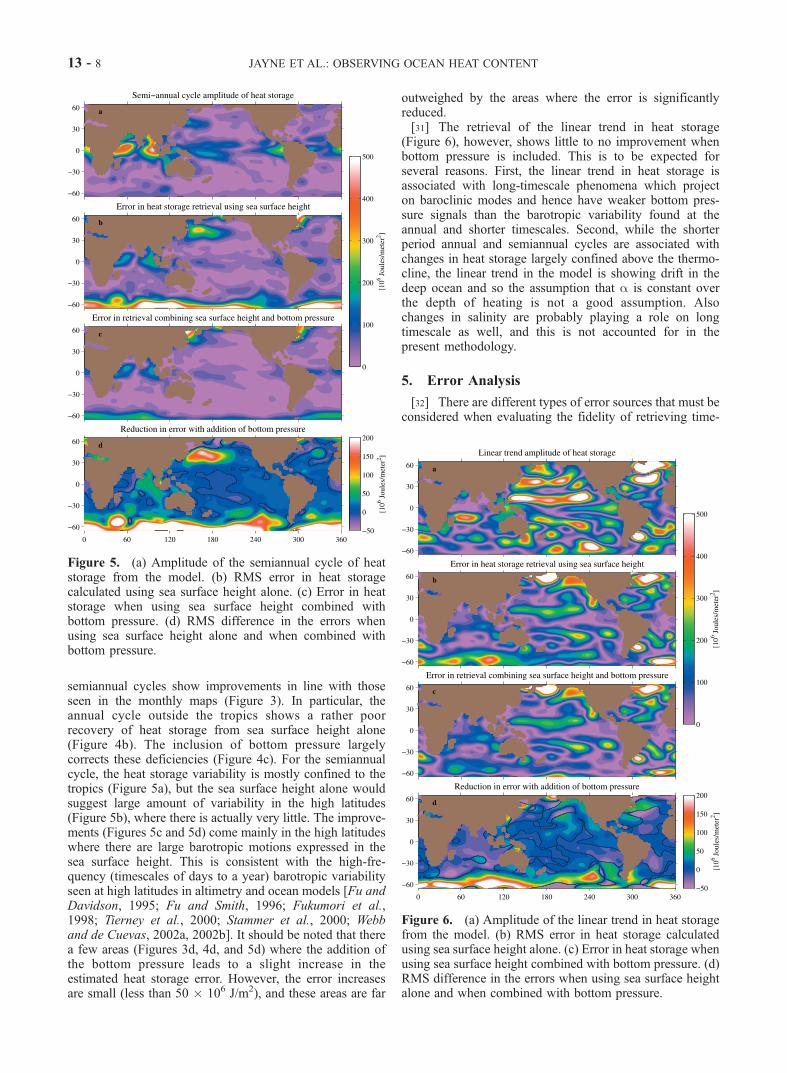
semiannual cycles show improvements in line with thoseseen in the monthly maps (Figure 3). In particular, theannual cycle outside the tropics shows a rather poorrecovery of heat storage from sea surface height alone(Figure 4b). The inclusion of bottom pressure largelycorrects these deficiencies (Figure 4c). For the semiannualcycle, the heat storage variability is mostly confined to thetropics (Figure 5a), but the sea surface height alone wouldsuggest large amount of variability in the high latitudes(Figure 5b), where there is actually very little. The improve-ments (Figures 5c and 5d) come mainly in the high latitudeswhere there are large barotropic motions expressed in thesea surface height. This is consistent with the high-fre-quency (timescales of days to a year) barotropic variabilityseen at high latitudes in altimetry and ocean models [Fu andDavidson, 1995; Fu and Smith, 1996; Fukumori et al.,1998; Tierney et al., 2000; Stammer et al., 2000; Webband de Cuevas, 2002a, 2002b]. It should be noted that therea few areas (Figures 3d, 4d, and 5d) where the addition ofthe bottom pressure leads to a slight increase in theestimated heat storage error. However, the error increasesare small (less than 50 � 106 J/m2), and these areas are far

outweighed by the areas where the error is significantlyreduced.[31] The retrieval of the linear trend in heat storage

(Figure 6), however, shows little to no improvement whenbottom pressure is included. This is to be expected forseveral reasons. First, the linear trend in heat storage isassociated with long-timescale phenomena which projecton baroclinic modes and hence have weaker bottom pres-sure signals than the barotropic variability found at theannual and shorter timescales. Second, while the shorterperiod annual and semiannual cycles are associated withchanges in heat storage largely confined above the thermo-cline, the linear trend in the model is showing drift in thedeep ocean and so the assumption that a is constant overthe depth of heating is not a good assumption. Alsochanges in salinity are probably playing a role on longtimescale as well, and this is not accounted for in thepresent methodology.

5. Error Analysis

[32] There are different types of error sources that must beconsidered when evaluating the fidelity of retrieving time-

Figure 5. (a) Amplitude of the semiannual cycle of heatstorage from the model. (b) RMS error in heat storagecalculated using sea surface height alone. (c) Error in heatstorage when using sea surface height combined withbottom pressure. (d) RMS difference in the errors whenusing sea surface height alone and when combined withbottom pressure.

Figure 6. (a) Amplitude of the linear trend in heat storagefrom the model. (b) RMS error in heat storage calculatedusing sea surface height alone. (c) Error in heat storage whenusing sea surface height combined with bottom pressure. (d)RMS difference in the errors when using sea surface heightalone and when combined with bottom pressure.


variable ocean heat content from altimetry and satellitegravity observations. There are measurement errors whicharise from noise processes in the observation of sea surfaceheight from the altimeters and bottom pressure fromGRACE, and there are methodology errors which arise fromthe assumptions and simplifications that were made to arriveat (26) to estimate heat storage from the observable quanti-ties. These can be further grouped into errors that are reducedby the introduction of the GRACE data, errors that areincreased by using GRACE data and errors that are essen-tially unchanged. The quantitative error estimates in thefollowing discussion are based on the ocean general circu-lation model output and a few ancillary data sets. The errorpropagation was performed using simulated GRACE andaltimeter data based on the ocean model output; a global,gridded map of continental water storage over all regionsexcept Antarctica from Shmakin et al. [2002]; of changes insnow mass over Antarctica using monthly, gridded, accu-mulation fields generated by the CSM-1 climate modeldeveloped at the National Center for Atmospheric Research[see, e.g., Briegleb and Bromwich, 1998]; of errors inatmospheric pressure over land (as by Wahr et al. [1998]);and of GRACE measurement errors, using error estimatesprovided by B. Thomas and M. Watkins (personal commu-nication, 1998) [see also Wahr et al., 1998; Jet PropulsionLaboratory, 2001]. While the numbers would vary if adifferent time period were analyzed or different forcing datasets were used, they do provide an assessment of the relativesizes of the different error sources. The reported errorsrepresent the areal average over the ocean from 1 offshoreof the coast within the latitude range 66S to 66N.

5.1. Measurement Errors

5.1.1. Altimetry Sampling Errors[33] Altimetric measurements from TOPEX have high

accuracy, with a point RMS error of about 3 cm [Wunschand Stammer, 1998]. In this error analysis, we assume themajority of the error is due to residual orbit error. Thisassumption leads to the most pessimistic error estimate,since it assumes the measurement errors for a single satellitepass are correlated, so that spatial averaging does little toreduce them. Therefore, to estimate the number of inde-pendent samples within a given averaging disk, the numberof degrees of freedom (N ) was estimated using the weightednumber of crossovers within the Gaussian average over amonth time span. The number of crossovers within theGaussian averaging area for a given time span is equal tothe square of half the number of satellite passes. Averagedover a large area, such as that encompassed by a severalhundred kilometer disk, these errors are reduced by 1/

ffiffiffiffiN

p.

For a single month, this results in an average RMS error of106 � 106 J/m2 in the retrieval of heat content (orequivalently, 40 W/m2 in terms of a time rate of changeof heat content) for a 500 km half-width averaging kernel.For 5 years of data, this source accounts for an error in theamplitude of the annual cycle of about 8 W/m2. This errorsource could be reduced somewhat by using multiple datasources (i.e., Jason plus Envisat and Geosat Follow-On);however, it is present whether or not GRACE data are used.5.1.2. Inverted Barometer Correction Error[34] One of the largest corrections made to the sea

surface height measured from altimetry is for the inverted

barometer response of the ocean to atmospheric pressurevariations [Wunsch and Stammer, 1997]. It is based on themean sea level pressure derived from operational andreanalysis products from the National Center for Environ-mental Prediction (NCEP) or the European Centre forMedium-Range Weather Forecasts (ECMWF). These modelproducts have errors and biases, but a detailed errorestimation of these product’s accuracy over the ocean hasnot been performed. However, over land the results indicatethat the pressure is good to about 0.5 mbar [Velicogna et al.,2001]. For the present purposes, as a measure of the errorwe take the RMS difference between the NCEP andECMWF surface pressure products divided by

ffiffiffi2

p, as by

Wahr et al. [1998]. Translated into a heat storage error,errors in the inverted barometer correction introduce anRMS error of 77 � 106 J/m2 (29 W/m2) for the monthlyheat storage estimates, and 3 W/m2 for the annual cycle.Figure 7a shows the monthly RMS of the heat content errorarising from satellite altimetry errors sources, includingerrors in the inverted barometer and orbit error. The largeerrors, especially near Antarctica are due to errors in theinverted barometer correction.

Figure 7. (a) The monthly RMS error arising fromsatellite altimetry errors sources. (b) The monthly RMSerror arising from GRACE error sources. (c) The monthlyRMS error from the thermal expansion coefficient. (d) Themonthly RMS error from the neglect of the halinecontribution to steric sea surface height.


5.1.3. GRACE Sampling Errors[35] GRACE measurement errors are more complicated,

as they are specified in spherical harmonic space. Thepurpose of the Gaussian spatial averaging we applied tothe model data to generate Figures 3–5, is to reduce thoseerrors to acceptable levels. For 5 years of data and a 500 kmaveraging radius, the RMS error in equivalent sea surfaceheight is about 1 mm (Table 1), which results in an error inthe monthly estimated heat storage of 20 � 106 J/m2 (8 W/m2). The error in the annual cycle from this source isslightly less than 1 W/m2.5.1.4. Postglacial Rebound[36] The large postglacial rebound signal in the North

Atlantic Ocean is problematic. Over the five year timescaleswe are considering, the postglacial rebound signal appears asa linear trend, so it will not affect the recovery of seasonal orother nonsecular signals. However, postglacial rebound is asignificant source of error when trying to use GRACE data toexamine the linear trend in bottom pressure. Unfortunately,the rebound is largest in the same places (i.e., the NorthAtlantic and Southern Oceans) where one might expect tosee the largest signal in bottom pressure arising from secularchanges in the ocean’s baroclinic structure. The limitedextent to which it can be modeled depends on the largelyunknown viscosity profile of the Earth’s mantle, and furtherresearch will be required to improve estimates of this errorsource. Taken together, all of the GRACE observation errorsamount to 63 � 106 J/m2 (24 W/m2) and the error in theannual cycle from GRACE observation errors is about 3 W/m2. Figure 7b shows the monthly RMS of the heat contenterror arising from satellite gravity errors, including errors inthe GRACE estimated geoid and leakage from other signalsuch as the hydrology signal over land and post glacialrebound.5.1.5. Leakage From Continental Hydrological Cycle[37] Leakage from the large hydrology signal over land

(e.g. groundwater storage) will contaminate the retrievalof GRACE signals close to the coast. However, coastalareas are also influenced by salinity effects from riverrunoff, and those effects have been ignored in ourderivation of (21) and (26). Furthermore, the currentgeneration of altimeters has poor data retrieval very closeto the coasts. The implication, then, is that leakage ofgravity signals from land will not be a large detriment tousing the GRACE data. Furthermore, the contaminationfrom the land hydrology can be significantly reducedusing the methodology described by Wahr et al. [1998,equations (35)–(39)], and useful bottom pressure valuesGRACE will likely be obtainable to within about 100 kmfrom the coast.[38] It is important to understand the tradeoffs between

the smoothing length scale and GRACE measurementerrors, as well as the extent of the leakage from hydro-logical signals over land. Generally, the smaller thesmoothing radius the better, as it improves spatial reso-lution, and reduces the area affected by leakage of thecontinental signals (though this signal can be significantlyreduced as described by Wahr et al. [1998]). While theleakage of the hydrology signal over land is decreased byreducing the averaging radius, smaller averaging radii areassociated with larger GRACE measurement errors. There-fore an optimal averaging area is problem dependent. To

illustrate the effect of the smoothing radius on the heatstorage estimation errors, a range of smoothing radii from100–1000 km were used to recompute the heat contentretrieval error as a function of smoothing radius (Figure 8).Plotted are the globally averaged RMS of the heat contentsignal (dotted line), the estimated error using noise-freeand noisy sea surface height alone (black dashed and solidlines respectively), and the estimated error using noise-freeand noisy GRACE observations (gray dashed and solidline respectively). It is readily seen that in general thelarger the averaging radius the lower the errors. However,at large averaging radii the time-varying heat contentsignal gets smeared out and weakened, and near the coaststhe error from the hydrology signal leakage is increased.At the smallest averaging radii, GRACE measurementerrors make the estimated heat content unusable. For thedetermination of heat storage, it is found that a 500-kmaveraging radius balances the errors introduced fromaltimetry and GRACE, while not leading to excessivecontamination by the land hydrology signal, and notoverly smoothing the desired heat content signal.

5.2. Methodology Errors

[39] Beyond the errors in estimation of heat storage fromobservational noise sources, there are errors introduced dueto some of the assumptions made.5.2.1. Thermal Expansion Coefficient Errors[40] The thermal expansion coefficient is not constant

over the depth that the heating is occurring as was assumedin deriving (18). Furthermore, a was calculated from themonthly mean sea surface temperature and salinity. Whenreal data from the GRACE mission is available along withaltimeter data from the ongoing missions, the thermalexpansion coefficient will be calculated from the climato-logical surface temperature and salinity fields [Levitus et al.,1994; Levitus and Boyer, 1994] or remotely sensed seasurface temperature [i.e., Reynolds and Smith, 1994]. Theseassumptions introduce errors into the estimation of the heat

Figure 8. Error in heat storage estimate averaged over theglobal ocean as a function of the averaging radius.


storage. We use the model output for a and T, and estimatethe error as

H 0err q;f; tð Þ ¼ rcp

a0

Z h

h

a q;f; z; tð ÞT 0 q;f; z; tð Þ dz a0 q;f; tð ÞZ h

h

T q;f; z; tð Þ dz �

ð27Þ

We find that the assumption of a depth independent thermalexpansion coefficient introduces a globally averaged RMSerror in the monthly estimated heat storage of 109� 106 J/m2

(41 W/m2) and the error in the estimated annual cycle for 5years of data is about 10 W/m2. The contribution to the errorbudget from the assumption of a depth independent thermalexpansion coefficient is shown in Figure 7c.5.2.2. Haline Effects[41] The contribution to the steric sea surface height by

haline contraction was also neglected in the estimationprocedure, introducing another error source. The contribu-tion to the error budget from this assumption is estimated as,

H 0err q;f; tð Þ ¼ rcp

a0

Z h

h

bS0 dz: ð28Þ

The neglect of the haline contribution to the steric sea surfaceheight contributes an error of about 139 � 106 J/m2

(53 W/m2) and the error in the annual cycle is about11 W/m2. Figure 7d shows the monthly RMS of the errorarising from the neglect of the haline contribution to thesteric sea surface height.[42] Taken together, the methodology errors account for

an error of about 15 W/m2 in the estimate of the annualcycle. The errors inherent in the methodology then accountfor about 3 times the error variance introduced by the totalof the observational errors at 9 W/m2. Overall, this indicatesthat the estimation of heat storage using a 500 km averagingradius will not be vastly improved by either additional seasurface height data or from more precise satellite gravityobservations. Rather, observations of salinity (eitherremotely sensed or in situ) would be of most benefit.Modification of the estimation methodology to break theconstraint of a depth independent thermal expansion coef-ficient would also be of benefit. If GRACE performs tospecification, it is expected that higher-precision satellitegravity missions will be flown in the future. This increasedprecision would allow for a decreased smoothing radius,and therefore permit higher spatial resolution in the heatstorage estimates.

6. Conclusions

[43] The combination of satellite altimetry combined withbottom pressure observations (i.e., from the GRACE mis-sion) offers a superior method for estimating the ocean’stime-varying heat storage over using altimetry alone. Spe-cifically, it significantly reduces errors associated withbarotropic variability at high latitudes, which would other-wise dominate the errors in the inferred steric heightvariability in those regions. For the month-to-month varia-tions in heat storage, with a 500 km half-width averaging

kernel, the error in the estimated heat content from altimetryalone is about 380 � 106 J/m2 compared to 200 � 106 J/m2

for the heat content computed from hydrographic profiles.When bottom pressure observations from satellite gravityare included, the error is reduced to 280 � 106 J/m2, morecomparable to using hydrography. However, while theaddition of bottom pressure data does significantly reducethe errors in the estimated heat content, there are stillsignificant limitations that must be addressed before thismethodology can equal the accuracy of in situ measure-ments. In particular, the addition of salinity observations,either in situ or remotely sensed, would be of great benefit.[44] The challenge now will be to combine in situ

observations of temperature and salinity from the profilingfloats to be used in the Argo float program [Roemmich andOwens, 2000] to provide ground truth by which to test themethod described here. Furthermore, satellite altimetry,GRACE and Argo will complement each other to providea more complete Global Ocean Observing System. The insitu observations from the Argo floats should allow moreaccurate calculation of the thermal expansion coefficient, aswell as take into account the haline effects in the steric seasurface height. However, the float data will suffer fromsparse coverage and eddy aliasing problems. At the sametime, the satellite observations should allow for a morecomplete spatial coverage to fill in gaps in the float data. Sothe combination should provide a more complete andreliable measure of the ocean heat storage. The resultingestimates of heat storage will place a strong constraint andconsistency check on the estimates of surface heat fluxproduced by the meteorological centers. Taken together, theaddition of GRACE to the ocean observation system willimprove the estimation of the time-varying heat storage andplay a fundamental role in the Global Climate ObservingSystem being deployed.

[45] Acknowledgments. We would like to thank Andrey Shmakin,Chris Milly, and Krista Dunne for providing the output of their global,gridded water storage data set; and Dazhong Han for providing his elasticLove numbers. This work was partially supported by NASA grant NAG5-7703 and JPL contract 1218134 to the University of Colorado, JPL contract1234336 to the Woods Hole Oceanographic Institution, and by the NSFthrough its sponsorship of NCAR. This is Woods Hole OceanographicInstitution Contribution number 10840.

ReferencesBriegleb, B. P., and D. H. Bromwich, Polar climate simulation of theNCAR CCM3, J. Clim., 11, 1270–1281, 1998.

Chambers, D. P., B. D. Tapley, and R. H. Stewart, Long-period ocean heatstorage rates and basin-scale heat fluxes from TOPEX, J. Geophys. Res.,102, 10,525–10,533, 1997.

Chambers, D. P., B. D. Tapley, and R. H. Stewart, Measuring heat-sto-rage changes in the Equatoral Pacific: A comparison between TOPEXaltimetry and TAO buoys, J. Geophys. Res., 103, 18,591–18,597,1998.

Chao, B. F., and R. S. Gross, Changes in the Earth’s rotation and low-degree gravitational field induced by earthquakes, Geophys. J. R. Astron.Soc., 91, 569–596, 1987.

Chao, Y., and L.-L. Fu, A comparison between the TOPEX/Poseidon dataand a global ocean general circulation model during 1992 – 1993,J. Geophys. Res., 100, 24,965–24,976, 1995.

Chen, J. L., C. K. Shum, C. R. Wilson, D. P. Chambers, and B. D. Tapley,Seasonal sea level change from TOPEX/Poseidon observations and ther-mal contribution, J. Geodesy, 72, 638–647, 2000.

Cheney, R. E., L. Miller, R. Agreen, N. Doyle, and J. Lillibridge, TOPEX/Poseidon: The 2-cm solution, J. Geophys. Res., 99, 24,555–24,564,1994.


Dickey, J. O., et al., Satellite Gravity and the Geosphere: Contributions tothe Study of the Solid Earth and Its Fluid Envelope, Natl. Acad. Press,Washington, D.C., 1997.

Dukowicz, J., and R. D. Smith, Implicit free-surface method for the Bryan-Cox-Semtner ocean model, J. Geophys. Res., 99, 7991–8014, 1994.

Farrell, W. E., Deformation of the Earth by surface loads, Rev. Geophys.,10, 761–797, 1972.

Ferry, N., G. Reverdin, and A. Oschlies, Seasonal sea surface height varia-bility in the North Atlantic Ocean, J. Geophys. Res., 105, 6307–6326,2000.

Fu, L.-L., and D. B. Chelton, Large-scale ocean circulation, in SatelliteAltimetry and Earth Sciences, edited by L.-L. Fu and A. Cazenave, pp.133–169, Academic, San Diego, Calif., 2001.

Fu, L.-L., and R. A. Davidson, A note on the barotropic response of sealevel to time-dependent wind forcing, J. Geophys. Res., 100, 24,955–24,963, 1995.

Fu, L.-L., and R. D. Smith, Global ocean circulation from satellite altimetryand high-resolution computer simulation, Bull. Am. Meteorol. Soc., 77,2625–2636, 1996.

Fukumori, I., R. Raghunath, and L.-L. Fu, Nature of global large-scale sealevel variability in relation to atmospheric forcing: A modeling study,J. Geophys. Res., 103, 5493–5512, 1998.

Gent, P. R., and J. C. McWilliams, Isopycnal mixing in ocean circulationmodels, J. Phys. Oceanogr., 20, 150–155, 1990.

Gill, A. E., Atmosphere-Ocean Dynamics, Academic, San Diego, Calif.,1982.

Gill, A. E., and P. P. Niiler, The theory of the seasonal variability in theocean, Deep Sea Res., 20, 141–178, 1973.

Greatbatch, R. J., A note on the representation of steric sea level in modelsthat conserve volume rather than mass, J. Geophys. Res., 99, 12,767–12,771, 1994.

Hendricks, J. R., R. R. Leben, G. H. Born, and C. J. Koblinsky, Empiricalorthogonal function analysis of global TOPEX/Poseidon altimeter dataand implications for detection of global sea level rise, J. Geophys. Res.,101, 14,131–14,145, 1996.

Hughes, C. W., C. Wunsch, and V. Zlotnicki, Satellite peers through theoceans from space, Eos Trans. AGU, 81, 68, 2000.

Jekeli, C., Alternative methods to smooth the Earth’s gravity field, Tech.Rep. 327, Dep. of Geod. Sci. and Surv., Ohio State Univ., Columbus,1980.

Jet Propulsion Laboratory, GRACE science and mission requirements docu-ment, GRACE 327-200, Rev. D, Tech. Rep. JPL Publ. D-15928, JetPropul. Lab., Pasadena, Calif., 2001.

Johnson, T. J., C. R. Wilson, and B. F. Chao, Nontidal oceanic contributionsto gravitational field changes: Predictions of the Parallel Ocean ClimateModel, J. Geophys. Res., 106, 11,315–11,334, 2001.

Large, W. G., J. C. McWilliams, and S. C. Doney, Oceanic vertical mixing:A review and a model with nonlocal boundary layer parameterization,Rev. Geophys., 32, 363–403, 1994.

Large, W. G., G. Danabasoglu, S. Doney, and J. C. McWilliams, Sensitivityto surface forcing and boundary layer mixing in a global ocean model:Annual mean climatology, J. Phys. Oceanogr., 27, 2418–2447, 1997.

Leuliette, E. W., and J. M. Wahr, Coupled pattern analysis of sea surfacetemperature and TOPEX/Poseidon sea surface height, J. Phys. Oceanogr.,29, 599–611, 1999.

Levitus, S., and T. Boyer, World Ocean Atlas 1994, vol. 4, Temperature,NOAA Atlas NESDIS, vol. 4, 129 pp., Natl. Oceanic and Atmos. Admin.,Washington, D.C., 1994.

Levitus, S., R. Burgett, and T. Boyer, World Ocean Atlas 1994, vol. 3,Nutrients, NOAA Atlas NESDIS, vol. 3, 129 pp., Natl. Oceanic and At-mos. Admin., Washington, D.C., 1994.

Maes, C., Estimating the influence of salinity of sea level anomaly in theocean, Geophys. Res. Lett., 25, 3551–3554, 1998.

Polito, P. S., O. T. Sato, and W. T. Liu, Characterization and validation ofheat storage variability from TOPEX/Poseidon at four oceanographicsites, J. Geophys. Res., 105, 16,911–16,921, 2000.

Ponte, R. M., A preliminary model study of the large-scale seasonal cycle inbottom pressure over the global ocean, J. Geophys. Res., 104, 1289–1300, 1999.

Repert, J. P., J. R. Donguy, G. Elden, and K. Wyrtki, Relations between sealevel, thermocline depth, heat content, and dynamic height in the tropicalPacific Ocean, J. Geophys. Res., 90, 11,719–11,725, 1985.

Reynolds, R. W., and T. M. Smith, Improved global sea surface tem-perature analyses using optimum interpolation, J. Clim., 7, 929–948,1994.

Roemmich, D., and W. B. Owens, The argo project: Global ocean observa-tions for understanding and prediction of climate variability, Oceanogra-phy, 13, 45–50, 2000.

Sato, O. T., P. S. Polito, and W. T. Liu, Importance of salinity measurementsin the heat storage estimation from TOPEX/Poseidon, Geophys. Res.Lett., 27, 549–551, 2000.

Shmakin, A. B., P. C. D. Milly, and K. A. Dunne, Global modeling of landwater and energy balances, 3, Interannual variability, J. Hydrometeorol.,3, 311–321, 2002.

Smagorinsky, J., General circulation experiments with the primitive equa-tions, I, The basic experiment, Mon. Weather Rev., 91, 99–164, 1963.

Smith, R. D., and J. C. McWilliams, Anisotropic horizontal viscosity forocean models, Ocean Modell. 5, Hooke Inst., Oxford Univ., Oxford,U. K., 2002.

Stammer, D., Steric and wind-induced changes in TOPEX/Poseidon large-scale sea surface topography observations, J. Geophys. Res., 102,20,987–21,009, 1997.

Stammer, D., C. Wunsch, and R. Ponte, De-aliasing of global high fre-quency barotropic motions in altimeter observations, Geophys. Res. Lett.,27, 1175–1178, 2000.

Swenson, S., and J. Wahr, Methods for inferring regional surface-massanomalies from Gravity Recovery and Climate Experiment (GRACE)measurements of time-variable gravity, J. Geophys. Res., 107(B9),2193, doi:10.1029/2001JB000576, 2002.

Tierney, C., J. Wahr, F. Bryan, and V. Zlotnicki, Short-period oceaniccirculation: Implications for satellite altimetry, Geophys. Res. Lett., 27,1255–1258, 2000.

Tomczak, M., and J. S. Godfrey, Regional Oceanography: An Introduction,Pergamon, New York, 1994.

Velicogna, I., J. Wahr, and H. Van den Dool, Can surface pressure be usedto remove atmospheric contributions from GRACE data with sufficientaccuracy to recover hydrological signals?, J. Geophys. Res., 106,16,415–16,434, 2001.

Vivier, F., K. A. Kelly, and L. Thompson, Contributions of wind forcing,waves and surface heating to sea surface height observations in the Pa-cific Ocean, J. Geophys. Res., 104, 20,767–20,788, 1999.

Wahr, J., M. Molenaar, and F. Bryan, Time variability of the Earth’s gravityfield: Hydrological and oceanic effect and their possible detection usingGRACE, J. Geophys. Res., 103, 30,205–30,229, 1998.

Wahr, J. M., S. R. Jayne, and F. O. Bryan, A method of inferring changes indeep ocean currents from satellite measurements of time variable gravity,J. Geophys. Res, doi:10.1029/2001JC001274, in press, 2002.

Wang, L., and C. Koblinski, Can the TOPEX/Poseidon altimetry data beused to estimate air-sea heat flux in the North Atlantic, Geophys. Res.Lett., 24, 139–142, 1997.

Webb, D. J., and B. A. de Cuevas, An ocean resonance in the southeastPacific, Geophys. Res. Lett., 29(14), 1252, doi:10.1029/2001GL014259,2002a.

Webb, D. J., and B. A. de Cuevas, An ocean resonance in the Indian sectorof the Southern Ocean, Geophys. Res. Lett., 29(14), 1664, doi:10.1029/2002GL015270, 2002b.

White, W. B., and C.-K. Tai, Inferring interannual changes in the globalupper ocean heat storage from TOPEX altimetry, J. Geophys. Res., 100,24,943–24,954, 1995.

Wunsch, C., and D. Stammer, Atmospheric loading and the oceanic ‘‘in-verted barometer’’ effect, Rev. Geophys., 35, 79–107, 1997.

Wunsch, C., and D. Stammer, Satellite altimetry, the marine geoid, and theoceanic general circulation, Annu. Rev. Earth Planet. Sci., 26, 219–253,1998.

F. O. Bryan, Climate and Global Dynamics Division, National Center for

Atmospheric Research, PO Box 3000, Boulder, CO 80307-3000, USA.([email protected])S. R. Jayne, Physical Oceanography Department, Woods Hole Oceano-

graphic Institution, MS 21, Woods Hole, MA 02543-1541, USA.([email protected])J. M. Wahr, Department of Physics, University of Colorado, Campus Box

390, Boulder, CO 80309-0390, USA. ([email protected])


observing ocean heat content using satellite gravity and...

Documents