1

Observer-based Engine Cooling Control System (OBCOOL)

Project Proposal

Students: Andrew Fouts & Kurtis Liggett

Advisor: Dr. Gary Dempsey

Date: December 09, 2010

2

Introduction Control systems exist in many applications today, from home thermostats and

vehicle cruise controls to engine temperature regulation and missile-guidance systems. Many control system designs exist, and one of the newer, more sophisticated concepts in modern control systems is the concept of observers. Observers are algorithms used to predict a system’s response. While complex, observers are a powerful addition to a control system and greatly improve the system’s performance [1].

Our project will consist of researching observer-based control systems and applying this knowledge to design closed-loop controllers for velocity control and temperature regulation of an engine cooling system. The controllers will be implemented using DSP boards with Simulink auto-code generation. In addition, energy management and controller performance will be evaluated. Goals

General o Learn software packages for auto-code generation and real-time control

via Simulink/DSP interface o Design energy management control system in Simulink environment to

regulate voltage/current to each subsystem o Evaluate controller performance based on system accuracy, speed, and

energy use o Determine the limitations of the Simulink/DSP interface in terms of real-

time execution and program memory

Thermal Control o Understand DSP/cooling system hardware interface o Obtain a mathematical model of the cooling system o Design closed-loop controllers for temperature regulation of cooling

system using observer-based system and energy management software for control of pump and fan

o Provide temperature data to Engine DSP via CAN bus interface

Engine Control o Understand DSP/motor hardware interface o Design software for PWM generation and velocity calculation from rotary

encoder o Design closed-loop controllers for velocity control using observer-based

system o Design observer-based system to acquire low noise current and velocity

signal with minimal phase lag o Design energy management software to limit engine power output based

on Thermal DSP data via CAN bus interface and motor power calculation based on observer outputs of velocity and current

o Provide engine data to Thermal DSP via CAN bus

3

Functional Description The engine control workstation consists of the following subcomponents:

Engine model simulated by a motor-generator system

Variable load for engine

Cooling system consisting of a fan, radiator, cooling block, reservoir, pump, flow meter, and three temperature sensors

Two eZdsp F2812 DSP boards

PC software GUI (MATLAB/Simulink and Code Composer)

A closed-loop control system will be implemented for both the engine system and the thermal system. While the initial control systems will be developed using EE 431 (“classical”) control methods, the final system will incorporate observers to improve the systems’ responses. The overall system functions as follows:

1. Using the PC GUI, the user sets the system inputs (engine RPM, etc.) for the engine.

2. The PC sends data to the DSP boards through Code Composer. 3. The engine control DSP board sets the engine RPM to the desired value using

the implemented control algorithm and PWM signals. 4. The thermal control DSP board adjusts the temperature of the engine by

changing the pump & fan motor speeds using the implemented control algorithm and PWM signals.

5. The engine control output information and the thermal control output information are sent back to the PC and are displayed in the GUI.

Inputs Outputs

RPM RPM

Power Limiter Current

Power dissipated

Output power

Observer RPM

Observer current

Inputs Outputs

Temperatures Temperature of radiator inlet

Temperature of radiator outlet

Engine block temperature

Power of each subsystem

Observer temperatures

Inputs / Outputs

Thermal

Engine

Table 3-1 System Inputs/Outputs

4

Functional Description, cont.

Matlab Simulink Real-Time Workshop

Code Composer

F28212 eZdsp Board

PC

Link to Code Composer

Fig. 4-1 General Software Flow Chart [2]

The eZdsp F2812 DSP board will be used in both the motor control subsystem

and the cooling control subsystem. The design and implementation of these control systems is done through the PC. The software packages that will be used are MATLAB, Simulink and Realtime Workshop, and Code Composer 3.

- MATLAB is the main program associated with the project. It will be the host to other software, such as Simulink.

- Simulink is used to build the models of the subsystems. - The Realtime Workshop is used to convert the Simulink model into C code

using Code Composer. - Link to Code Composer is used to link the Real-time Workshop to Code

Composer

5

System Block Diagrams

Engine model/Cooling system

CAN bus communicationEngine control

(TMS320F2812 DSP board)

Thermal control(TMS320F2812 DSP

board)

Windows PC #1 Windows PC #2

Velocity

Engine PWM

Current

Pump/Fan PWM

Code Composer Code Composer

User Input User Input

Sensor Temperatures

Fig. 5-1

Overall Block Diagram

The overall system consists of the plant (engine/cooling system), the engine & thermal controls (DSP boards), and two Windows PCs with Code Composer interfaces. The user’s input will be sent to the DSP boards for processing. After the boards have executed the user’s commands, the resulting output will be sent back to the Code Composer interface and displayed.

6

System Block Diagrams, cont.

Motor Generator

LoadPower Resistor

Rotary Encoder

MotorDSP Board

External Hardware

H-Bridge

Fig. 6-1

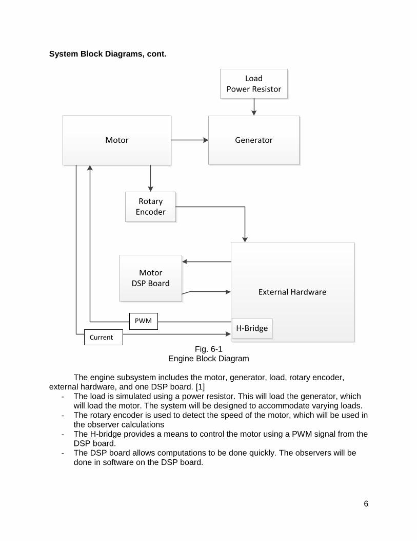
Engine Block Diagram

The engine subsystem includes the motor, generator, load, rotary encoder, external hardware, and one DSP board. [1]

- The load is simulated using a power resistor. This will load the generator, which will load the motor. The system will be designed to accommodate varying loads.

- The rotary encoder is used to detect the speed of the motor, which will be used in the observer calculations

- The H-bridge provides a means to control the motor using a PWM signal from the DSP board.

- The DSP board allows computations to be done quickly. The observers will be done in software on the DSP board.

PWM

Current

7

System Block Diagrams, cont.

Pump Motor

ThermalDSP Board

External Hardware

Fan MotorFan Control Hardware

Pump Control Hardware

Radiator inlet temp. sensor

Radiator outlet temp. sensor

Engine block temp. sensor

Fig. 7-1

Thermal Control Block Diagram

The thermal subsystem includes the fan & pump motors, hardware for controlling each motor, three temperature sensors, and one DSP board. [2]

- The temperature sensors each contain one thermistor for measuring the temperature. The thermistor’s resistance varies with temperature, causing the voltage output of each sensor to change.

- The DSP board converts the voltage levels from the temperature sensors into digital values and calculates the required fan/pump motor speeds required to cool the system.

- The DSP board outputs a PWM signal (through the external hardware) to the fan/pump motors and adjusts their speed.

- The DSP board allows computations to be done quickly. The observers will be done in software on the DSP board.

8

Circuit Schematics

Fig. 8-1

High Level Schematic of Power Electronics [2]

The circuitry of figure 8-1 is of the power electronics for both the engine and thermal subsystems. The main components of the engine subsystem are integrated into the left half of the board. The thermal control components are integrated into the right half of the board. Each subsystem has been isolated from the other and, therefore, each subsystem also has its own ground.

9

Circuit Schematics, cont.

Fig. 9-1 Engine Control Circuitry [2]

The circuit schematic for the engine control subsystem is shown in figure 9-1.

The components include the motor, a DSP board, a 3.3V to 5V level shifter, an H-bridge, and A/D conditioning circuitry. This circuitry has already been implemented in a previous senior project.

10

Circuit Schematics, cont.

Fig. 10-1

Thermal Control Circuitry [2]

Figure 10-1 shows the circuit components for the thermal control subsystem. The components include a 3.3V to 5V level shifter, transistors, and A/D conditioning circuitry. This circuitry has been implemented in a previous senior project.

11

Functional Requirements & Performance Specifications Engine control system The engine control system will go through multiple designs. A basic proportional controller will be implemented first, followed by PI & PID controllers. The final controller will be observer-based. The final engine control system shall meet the following specifications using a step input:

Steady-state error = ± 5 RPM

Percent overshoot ≤ 10%

Rise time ≤ 30 ms

Settling time ≤ 100 ms

Phase margin = 45° The data for these specifications will be collected for each method of control. This data will then be compared to make conclusions on the advantages and disadvantages for each control method. Each method will then be implemented in the engine control system. Both theoretical and experimental data will be collected. The control method command input range will vary based on the method used. Thermal control system

The thermal control system will go through several design iterations. A basic proportional controller will be implemented first, followed by PI & PID controllers. The final controller will be observer-based. The final thermal system shall meet the following specifications using a step input:

Steady-state error = ±2° Celsius

Percent overshoot ≤ 25%

Rise time ≤ 2 seconds

Settling time ≤ 10 seconds

Phase margin = 45° During system operation, the thermal control system shall ensure that the engine temperature remains below 40° C (104° F). The power consumed by the thermal control system shall remain at a minimum level. Each controller method listed above will be tested against the defined requirements. The method that best meets these requirements will be used in the final thermal control system.

12

Preliminary Results Engine control system Preliminary simulations were done in MATLAB to develop and analyze the engine subsystem. A general model of the engine control subsystem was developed to get a sense of how the system works. The model is shown in figure 12-1.

Fig. 12-1

Engine Control System

The first component of the model was based on work done in the senior mini-project. The model of the Pittman motor had already been developed. This model is shown in figure 12-2.

Fig. 12-2

Pittman Motor Subsystem

The closed-loop poles of the subsystem shown in figure 12-2 become the open loop poles of the engine control loop. After plugging in values and manipulating the equations, the formula for the plant becomes equation 13-1:

Unity Feedback

5/3.3

level shifter

motor_rpm

To Workspace1

v olts internal shaf t v elocity

Pittman Motor Model

bits_in v olts

PWMInput

In1 v olts

H-bridge

rad/sec motor_RPM

H

In1 Out1

Control Laws

1

internal shaft velocity

load

load

torque

To Workspace3

current

To Workspace2

T_f

Tf

1

J.s

ME side

Kv

Kv

Kt

Kt

1

La.s+Ra

EE side

B

B

1

volts

13

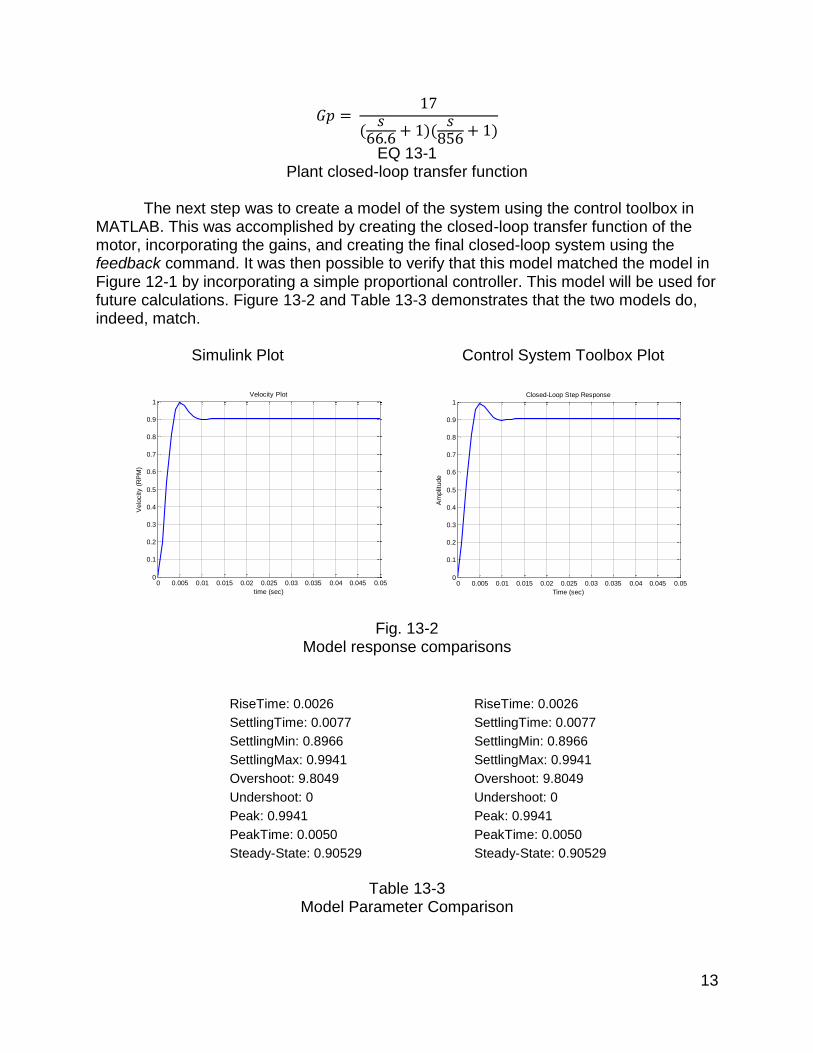
EQ 13-1 Plant closed-loop transfer function

The next step was to create a model of the system using the control toolbox in MATLAB. This was accomplished by creating the closed-loop transfer function of the motor, incorporating the gains, and creating the final closed-loop system using the feedback command. It was then possible to verify that this model matched the model in Figure 12-1 by incorporating a simple proportional controller. This model will be used for future calculations. Figure 13-2 and Table 13-3 demonstrates that the two models do, indeed, match. Simulink Plot Control System Toolbox Plot

Fig. 13-2

Model response comparisons

RiseTime: 0.0026 RiseTime: 0.0026

SettlingTime: 0.0077 SettlingTime: 0.0077

SettlingMin: 0.8966 SettlingMin: 0.8966

SettlingMax: 0.9941 SettlingMax: 0.9941

Overshoot: 9.8049 Overshoot: 9.8049

Undershoot: 0 Undershoot: 0

Peak: 0.9941 Peak: 0.9941

PeakTime: 0.0050 PeakTime: 0.0050

Steady-State: 0.90529 Steady-State: 0.90529

Table 13-3

Model Parameter Comparison

0 0.005 0.01 0.015 0.02 0.025 0.03 0.035 0.04 0.045 0.050

0.1

0.2

0.3

0.4

0.5

0.6

0.7

0.8

0.9

1

time (sec)

Velo

city (

RP

M)

Velocity Plot

0 0.005 0.01 0.015 0.02 0.025 0.03 0.035 0.04 0.045 0.050

0.1

0.2

0.3

0.4

0.5

0.6

0.7

0.8

0.9

1

Time (sec)

Am

plit

ude

Closed-Loop Step Response

14

A simple PWM signal was then tested on the engine cooling workstation to determine the time delay of the system. It was determined that the Code Composer graph could not sample at a fast enough rate to capture the percent overshoot or the time delay, so the time delay is assumed to be the 1ms delay programmed into the software. After determining the time delay of the system, the pade command was used in the control toolbox model to simulate time delay to get a more accurate representation of the system. Frequency domain analysis was determined to be the more suitable option in calculation the proportional gain term Kp. Thermal control system

The first step in the project was to set up the proper conversion for the system temperatures. A linear equation for the thermistor resistance versus temperature was created in order to implement the calculations for the temperature sensors in the control system. The linearization of the thermistor versus temperature can be seen in Fig. 14-1:

Fig. 14-1

Thermistor Linearization Graph

Next, a simple proportional and proportional-integral controller was created to confirm the basic operation of the system. With some tuning, the Kp and Ki were determined to be about 50 and about 0.0001, respectively. One of the problems encountered early on was integrator windup. While a limit block was used to handle the problem for now, a better solution may be needed in the future. The PI controller can be seen in Fig. 15-1:

y = -1743.7x + 60241

0

10000

20000

30000

40000

50000

60000

70000

Thermistor Chart

Resistance (Ohms)

Linear (Resistance (Ohms))

15

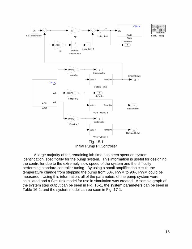
Fig. 15-1

Initial Pump PI Controller

A large majority of the remaining lab time has been spent on system identification, specifically for the pump system. This information is useful for designing the controller due to the extremely slow speed of the system and the difficulty performing standard controller tuning. By using a small amplification circuit, the temperature change from stepping the pump from 50% PWM to 90% PWM could be measured. Using this information, all of the parameters of the pump system were calculated and a Simulink model for use in simulation was created. A sample graph of the system step output can be seen in Fig. 16-1, the system parameters can be seen in Table 16-2, and the system model can be seen in Fig. 17-1:

CalcPWM

7

OutletVolts

6

InletVolts

5

RadiatorOutlet

4

RadiatorInlet

3

EngineBlock

2

EngineVolts

1

VoltsToTemp 2

VoltsIn TempOut

VoltsToTemp 1

VoltsIn TempOut

VoltsToTemp

VoltsIn TempOut

VoltsPer2

.00073

VoltsPer1

.00073

VoltsPer

.00073

Using limit 1

Using limitSetTemperature

25

PWM

C281 x

PWM

W2

Kp

50

Ki

.0001

F2812 eZdsp

Discrete

Transfer Fcn

z

z-1

ADC

C281 x

ADC

A0

A1

A2

16

Fig. 16-1

Sample of Pump PWM Step graph

Table 16-2 Pump System Parameters & Measurements

-0.45

-0.4

-0.35

-0.3

-0.25

-0.2

-0.15

-0.1

-0.05

0

0.05

0.1

0.3

21.0

41.7

62.4

83.2

3.9

24.6

45.3

66.0

86.8

7.5

28.2

48.9

69.6

810.4

11.1

211.8

412.5

613.2

814

14.7

215.4

416.1

616.8

817.6

18.3

219.0

419.7

620.4

821.2

21.9

222.6

4

Vt

Trigger

Settings

Rpot 44890

Fan PWM 100%

Value #1 PWM 50%

Value #2 PWM 90%

Gain

Test Before Step After Step Difference Rt #1 Rt #2 Difference Temp #1 Temp #2 Difference

#1 -0.244 -0.072 0.172 44454 44760.903 306.90143 29.05374 28.87773 0.17600585

#2 0.536 0.676 0.14 45862.87 46120.461 257.59066 28.24576 28.09803 0.147726468

#3 0.744 0.848 0.104 46246.11 46438.939 192.83356 28.02598 27.91539 0.110588714

Measurements

Test (time offset) (step offset) Td tp Peak value %OS ζ (damping ratio)

#1 1.1 -0.244 1.64 8.35 0.22 27.9% 0.376

#2 0.52 0.512 1.71 8.06 0.204 24.4% 0.41

#3 1.12 0.748 2 7.81 0.132 32.0% 0.341

Final value

0.172

0.164

0.1

Ts

13.34

13.41

12.49

17

Fig. 17-1

Pump System Simulink Model

The last portion of the project worked on thus far was implementing and tuning the PI controller based on the pump system model. The new Kp value was found to be 0.02, and the new Ki was found to be 0.00028. When these values are implemented in the physical system, however, the windup from the integrator caused issues again. An anti-windup system was implemented as seen in Fig. 17-2. This system effectively removed the integral windup, and the system is currently very responsive.

Fig. 17-2

Revised Pump PI Controller with Anti-Windup

To Workspace1

temperatureTo Workspace

t

Temp ScopeStep Pump /Thermistors

(.1477 /2.16 )/2.69

s +.458 s+.2042

Pump Voltage

ScopePost-controller Scope

PWM Scope

PWM LimitLevel Shifter

5/3.3

Kp

.02

Ki

.00028

Error Scope

Discrete

Transfer Fcn

z

z-1

DelayDSP Limit

Clock

Circuit Gain

2.69Temp Error

Temperature

Temperature

OutputPWM

7

IntegratorPWM

6

PWMBeforeSat

5

CalcPWM

4

RadiatorOutlet

3

RadiatorInlet

2

EngineBlock

1

Using limit

Unit Delay

1/z

SetTemperature

25

Pump range adjust

Input Output

PWM

C281 x

PWM

W1

W2

Level Shifter

100 /3.3

Kp

.02

Ki

.00028

Ka

50

Integrator

z

z-1

FanPWM

0

F2812 eZdsp

ADC

C281 x

ADC

A0

A1

A2A/D to Temp

A/D 1

A/D 2

A/D 3

Temp 1

Temp 2

Temp 3

UU'

18

Future Work Engine control system The design Kp value was successfully implemented on the engine cooling workstation. A PI control method will be implemented next. The design process will be similar to that of the proportional control. Observers will not be implemented until the other control methods are successfully implemented. Once the observer-based method is successfully implemented, all of the control methods will be compared and analyzed. The motor current reading will be integrated into the software model after the other steps have been completed. The engine control algorithm will then be designed to change velocity based on the engine current. If all of the previous steps have been completed successfully, the algorithm will be adjusted to communicate with the thermal cooling subsystem. Thermal control system

Once the PI controller for the pump system has been tuned properly, a control system for the radiator fan will be required next. This will follow a similar identification process as the pump; however, different methods of identifying parameters may be needed due to differences in the two systems. Once PI controllers have been implemented for both systems, work will begin on observers. After the observer-based method is successfully implemented, all of the control methods will be compared and analyzed. The thermal control algorithm will be designed to change pump and fan velocity based on the motor and system temperature. If all of the previous steps have been completed successfully, the algorithm will be adjusted to communicate with the engine control subsystem.

19

Future Work – Schedule

The schedule for the remaining time allotted for the project is shown below in Table 18-1:

Week Thermal Control System Engine Control System

1 P/PI Control PI Control

2 P/PI Control Feed-Forward Control

3 Alt. Advanced Control Feed-Forward Control

4 Observer-based Control Observer-based Control

5 Observer-based Control Observer-based Control

6 Observer-based Control Observer-based Control

7 Energy management & power

calculations

Engine governor & power dissipation

calculations

8 Energy management & power

calculations

Engine governor & power dissipation

calculations

9 CAN Bus CAN Bus

10 CAN Bus CAN Bus

11 Performance Evaluations Performance Evaluations

12 Performance Evaluations Performance Evaluations

13 Final Report & Presentation Final Report & Presentation

14 Final Report & Presentation Final Report & Presentation

Table 19-1

Project Schedule

20

Equipment List

The equipment used and costs for the project are listed below in Table 19-1. However, all of the equipment has already been purchased from previous projects. The only additional cost for this year’s work on the Engine Cooling System is the cost of two copies of Observers in Control Systems by George Ellis ($118 each).

Parts Description Cost

Fan $11

Radiator $29

Cooling Block $55

Reservoir and Pump $117

Flow meter $20

Coolant $15

Code Cathode $11

Temp Sensors (4) $40

Pittman Motors (2) $160

Motor Heat Sinks $20

Tubing, hose clamps $10

30Volt, 315 Watt Switching Power Supply $75

Advanced Motion Controls H-Bridge (6A) (donated) $350

Control and Interfacing Circuitry $30

eZdsp F2812 Texas Instruments DSP Boards (2) $975

Sub-total $1,918

Heat Sink Machine Shop Work 10 hours x $75/hr $750

Cooling Station Construction 40 hours x $75/hr $3,000

Software Installation 10 hours x $75/hr $750

Sub-total $4,500

Total $6,418

Table 20-1

Engine Cooling System Equipment & Costs

21

References [1] George Ellis. “Observers in Control Systems”, Academic Press, 2002. [2] Gary Dempsey. “Engine Control Workstation System Overview”, Electrical and Computer Engineering Department, Bradley University, September 2010 [3] Gary Dempsey. “Observer-based Engine/Cooling Control System”, Electrical and Computer Engineering Department, Bradley University, August 2010