Observations of entry and exit of Potential

Vorticity at the sea surface

Arnaud Czaja and Ute Hausmann

Department of Physics, Imperial College, London ∗

October 16, 2008

∗Author address: Dr. A. Czaja, Imperial College, Prince Consort Road, Huxley Build-

ing, Room 726; London SW7 2AZ, UK. tel: +44 (0)20 7594 1789 fax: +44 (0)20 7594

7900 email: a.czaja@imperial.ac.uk

1

2

Abstract

Although potential vorticity (PV) is central to many theories of the oceanic

circulation, the entry / exit of PV at the sea surface has not been thoroughly

discussed from an observational perspective. After clarifying the notion of

‘PV entry and exit’, and the mechanisms responsible for it, we present a

climatology of this quantity for the Northern Hemisphere.

It is found that surface PV loss over western boundary current regions and

their interior extension is a robust feature over the North Pacific and Atlantic

basins. At high latitudes, mechanical and diabatic effects act in concert in

the North Atlantic to drive net PV exit. In the Pacific, however, these effects

oppose each other and the net entry - exit of PV is more uncertain. At low

latitudes, surface winds are found particularly important in setting surface

PV exit in the Pacific, equatorward of the inter-tropical convergence zone.

3

1 Introduction

Potential vorticity (hereafter PV) is a central concept in physical oceanog-

raphy. Observationalists use it frequently as a way to trace water masses

(e.g., Talley and Mc Cartney, 1982); theoreticians put it at the core of our

understanding of how the ocean is set into motion (e.g., Rhines and Young,

1982; Luyten et al., 1983). Surprisingly, however, and even though maps

of potential vorticity have been frequently discussed (e.g., McDowell et al.,

1982; Keffer, 1985; Talley, 1988; O’Dwyer and Williams, 1997), the sources

and sinks of PV for the global ocean, and PV pathways from sources to sinks

in the oceanic interior are not known from an observational perspective.

Traditionally, and this mostly reflects the theoretical work done with

single or multi-layer quasigeostrophic models, anticyclonic windstress curl

is thought of as a sink of PV, being balanced by frictional PV gain at the

western boundary (e.g., Stommel, 1948) or surface PV gain due to cyclonic

windstress curl over the subpolar gyre (e.g., Marshall, 1984). Surface cooling

is also believed to be an important mechanism of PV loss (destruction of

stratification) and, conversely, surface heating (creation of stratification) a

mechanism of PV gain.

These mechanical and diabatic contributions to PV sources and sinks have

been elegantly put together in a single framework through the concept of ‘J-

vectors’, which represent the total (advective + non advective) transport

of potential vorticity within the ocean (Haynes and McIntyre, 1987; 1989;

4

Marshall and Nurser, 1992; Marshall, 2000). Denoting the potential vorticity

by Q (rigorous definitions are given below), the J-vector by J , density by ρ

and time by t, the conservation equation for PV can be written in flux form

as,

∂(ρQ)

∂t+ ∇ · J = 0 (1)

A major implication of (1) is that, in steady state, J must be non divergent.

In subtropical gyres, where Sverdrup dynamics predicts a downward advec-

tive transport in the interior of the ocean, one thus expects a surface entry

of PV into the ocean. Conversely, over subpolar gyres, the Sverdrup upward

advective transport must be matched by a surface PV exit out of the ocean!

(Note that these simple predictions omit the effect of PV transport by eddy

motions and, as a result, are only indicative of a possible dynamical regime).

It is our purpose to map from observations these surface entry / exit of

PV, discuss their meaning and the mechanisms responsible for their existence

(diabatic vs. mechanichal). To our knowledge, this has not yet been done

from observations, even though the concept of J-vectors has been used to

infer observational estimates of subduction rates over the North Atlantic

(Marshall et al., 1993), the sea surface PV entry / exit computed from an

ocean general circulation model of the North Atlantic (Marshall et al., 2001),

eddy - driven PV input into the thermocline (Csanady and Vittal, 1996), the

structure of the thermocline (Marshall, 2000), and, more recently, to discuss

the role of winds in forming mode waters (Thomas, 2005).

5

The paper is structured as follows. We present in section 2 some back-

ground on potential vorticity and the J-vector framework. In particular, we

wish to clarify the concept of surface PV entry and exit, that is, whether PV

is actually exchanged between the atmosphere and ocean at the sea surface.

In section 3, we present an observational estimate of the mechanical contribu-

tion to the air-sea PV flux, while a parallel effort is made in section 4 for the

diabatic contribution. The net PV flux is discussed in section 5. A discussion

and a conclusion section are offered in section 6 and 7, respectively.

2 Physics of J vectors

2.1 PV entry and exit at the sea surface

The framework for Ertel’s potential vorticity (PV) transport in geophysical

flows has been set out in various papers in both an oceanic and atmospheric

context (Haynes and McIntyre, 1987; 1989; Hoskins, 1991; Marshall and

Nurser, 1992; Csanady and Vittal, 1996; Marshall, 2000; Marshall et al.,

2001). Following Marshall and Nurser (1992), we define the potential vortic-

ity Q as

PV ≡ Q = −ξ ·∇σ

ρ(2)

in which ρ is seawater density, σ is the potential density (minus 1000 kgm−3)

and ξ is the absolute vorticity vector equal to the sum of the relative (ζ) and

planetary (2Ω) vorticity vectors. The minus sign in (2) is introduced so that

6

PV is positive in the Northern Hemisphere in regions where isopycnals are

flat (i.e., nearly horizontal). The unit of Q is m−1s−1 or, defining a unit of

‘PV-substance’ (pvs) as 1pvs = 1kgm−1s−1, Q can be expressed in units of

pvs/kg.

The flux of PV at a given position in space and time (in units of pvs m−2s−1),

hereafter denoted as the J-vector, or simply J , is given by (we refer the reader

to the above literature for a derivation of this formulae),

J = ρQu+ ξDσ

Dt+ F ×∇σ (3)

In eq. (3), u = (ui, vj, wk) denotes the three dimensional velocity field,

(i, j,k) being the local zonal, meridional and vertical unit vectors on the

sphere and (u, v, w) the associated velocity components, Dσ/Dt is the la-

grangian derivative of density, and F is the viscous body force per unit

mass,

F =Du

Dt+ 2Ω× u+

1

ρ∇p+ gk (4)

p being the pressure and g gravity. The first term on the r.h.s of (3) repre-

sents the advective transport of PV while the two remaining terms are non

advective and will be referred to in the following as the diabatic (involving

exchange of heat and water at the air-sea interface and thereby leading to

Dσ/Dt 6= 0) and mechanical (involving viscous effects, F 6= 0) components

of the J-vector, respectively.

The flux of PV across the sea surface (hereafter denoted by Js) is obtained

by dotting (3) with the local ocean surface normal. Approximating the latter

7

by k and setting w = 0 at the sea surface (z = 0), we obtain

Js = (ξDσ

Dt+ F ×∇σ)z=0 · k (5)

which, using further ξ · k ' f in which f is the Coriolis parameter (small

Rossby number approximation), is rewritten as

Js = f(Dσ

Dt)z=0 + (F ×∇σ)z=0 · k (6)

Introducing further the mechanical and diabatic components,

Jdiabs = f(Dσ

Dt)z=0 (7)

and

Jmechs = (F ×∇σ)z=0 · k (8)

we write

Js = Jdiabs + Jmechs (9)

As emphasized in Rhines (1993) care must be taken when relating Dσ/Dt

and F to air-sea buoyancy flux and surface windstress, respectively. Indeed,

the terms in (6) represent vertical divergence of turbulent buoyancy and mo-

mentum transport, not the turbulent transport themselves. An assumption

about the vertical structure of those fluxes in the mixed layer will have to

be made in order to relate directly Dσ/Dt and F to surface buoyancy fluxes

and windstress –see sections 3 and 4 below. Anticipating slightly on the

result, we identify the diabatic component of Js as reflecting the loss (gain)

of stratification when there is surface buoyancy loss (gain) by the ocean.

8

Conversely, the mechanical component of Js is interpreted as the loss (gain)

of stratification associated with a dense-to-light (light-to-dense) Ekman drift

–see Fig. 1.

2.2 Further background on J-vectors

Two results from the literature particularly help the analysis below. First, the

“impermeability theorem” (Haynes and McIntyre, 1987). The latter states

that the mass weighted PV content of any isopycnal layer can only be changed

through fluxes where the layer intersects a boundary. Sea surface PV entry -

exit is thus a component of the PV budget of isopycnal layers, the remaining

terms of this budget involving frictional effects where the isopycnal layers in-

tersect bathymetric features or the lateral boundaries of ocean basins (which

we have not attempted to estimate in this study). For this reason, the global

average of Js does not need to be zero. Net PV gain or loss at the sea surface

can be balanced by frictional sources and sinks at the basin boundaries or

bottom.

Another important result is that of Schaar (1993), who showed that,

irrespective of the nature of the PV transport (i.e., advective, frictionally

or diabatically induced), it must be equal, in a statistically steady state to

J = ∇B × ∇σ, in which B is the Bernoulli function. For typical ocean

conditions (e.g., Marshall and Nurser, 1992) this reduces to J ' fug ·∇σ,

in which ug is the geostrophic velocity. This relation thus allows a simple

9

interpretation of the net PV transport (Jmechs +Jdiabs ) as density gain following

the geostrophic flow (PV exit) or density loss following the geostrophic flow

(PV entry).

2.3 Is there air-sea exchange of PV between the ocean

and the atmosphere?

The J-vector framework shows that there is, in general, a non zero PV flux

at the air-sea interface. We wish to clarify here the physical meaning of this

flux, and whether it can be thought of as an exchange of PV between the

ocean and the atmosphere.

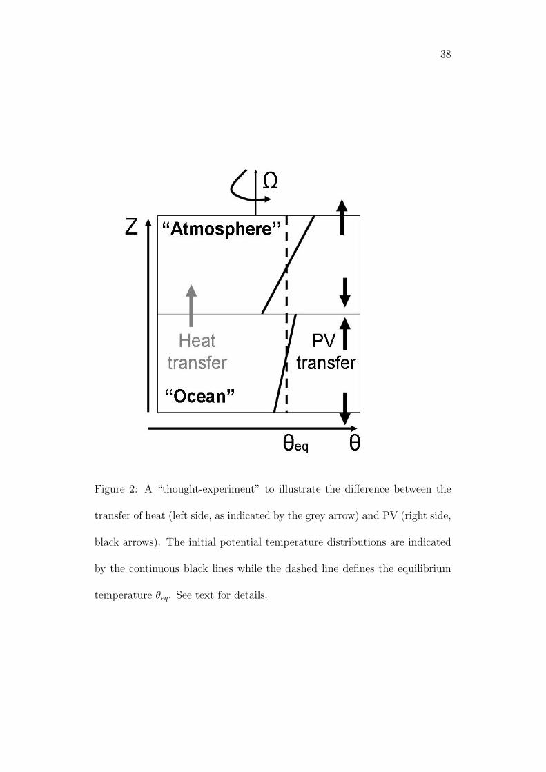
To do so, we consider a ‘thought’-experiment akin to that of Rhines

(1993), in which a rotating box is filled with two immiscible and (stably)

stratified fluids (simply characterized by potential temperature θ) with no

relative motion (Fig. 2). The upper fluid (loosely representing the atmo-

sphere) is initially colder than the lower fluid (the ocean) fluid at the inter-

face, and we let heat transfer and diffusive processes drive the system towards

a state of uniform temperature distribution θeq (Fig. 2, dashed line). There

is no exchange of heat with the surroundings as the box is assumed thermally

insulated form the surroundings.

From the PV point of view, each fluid is going from a state of high PV

(stratified) to a state of zero PV (no stratification at all), hence the J-vectors

must be directed outward for both fluid (PV loss). The impermeability

10

theorem (section 2.2) is a powerful tool to analyze more precisely the sense

of this PV transfer. Indeed, what happens is simply that each fluid “fills”

with the intermediate temperature class θeq, and the PV contained in the

warmer and colder layers is transported away from the central region with

those layers, as indicated by the black arrows. Of importance here is the

fact that the PV transport converges at the interface: the latter acts as a

reservoir in which PV is accumulated in this thought-experiment.

This simple example shows that rather than being exchanged between

ocean and atmosphere, like heat is (grey arrow in Fig. 2), PV transports

converge (or diverge) at the air-sea interface. For this reason, we will here-

after use the ‘PV entry/exit’ rather than ‘air-sea PV flux’ terminology.

3 Wind contribution to PV entry and exit

3.1 Methodology

To start with, we rewrite the non conservative force F in (3) as,

F ≡ 1

ρo

∂τ

∂z(10)

in which ρo is a reference density, and τ is a turbulent stress representing

the vertical transport of horizontal momentum by small scale processes. As

emphasized in section 2.1 some assumption about the turbulent momentum

fluxes must be made in order to relate the divergence of the latter to the

surface windstress. Considering that the mixed layer depth h characterizes

11

the vertical scale of the layer experiencing significant turbulent momentum

stresses, we assume ∂τ/∂z ' τ s/h, in which τ s = (τxi, τyj) is the surface

windstress vector. Assuming further that the density at the sea surface equals

the mixed layer density σm,

σz=0 ' σm (11)

we finally compute the mechanical contribution to Js as

Jmechs ' (τ sρoh×∇σm) · ~k (12)

Equation (12) makes the link with Schar’s formulation (section 2.1) par-

ticularly clear, with Jmechs simply representing the density advection by the

Ekman drift. This is one of term of the mixed layer density budget needed to

balance, in the mean, the geostrophic advection of density. To put a number

on this relationship, a stress τx = 0.1Nm−2 acting on mixed layer density

gradient ∂σm/∂y = 1kg m−3/1000km and a mixed layer depth h = 100m

leads to Jmechs ' 10−12pvs m−2s−1. As we will see, this number is typical of

observed entry/exit of PV at the sea surface.

In order to compute (12) a monthly windstress climatology was con-

structed over the 1960-1987 period from the NCEP-NCAR reanalysis (Kalnay

et al., 1996). The global monthly mixed layer depth climatology of Montegut

et al. (2004) was used to estimate h (temperature criterion). The mixed layer

density was computed by averaging potential density from the World Ocean

Atlas (Konkright et al, 2002) over the mixed layer. All PV flux calculations

shown in this paper were carried out with monthly climatologies on a 2×2

12

degrees longitude-latitude grid.

3.2 Northern Hemisphere maps

We first estimate, at a given location, the long term mean value of Jmechs

by annually averaging (12) at each oceanic gridpoint (Fig. 3). Entry of PV

(light shading) is seen in a large latitudinal band stretching from about 30 to

' 5−10. Exit of PV (dark shading) is seen poleward and equatorward of this

band. Unlike for quasi-geostrophic PV, the line separating mechanical PV

entry and exit does not coincide with the zero windstress curl line. Indeed,

because of the larger zonal than meridional winds, and the larger meridional

than zonal density gradients, the map in Fig. 3 is dominated by Jmechs '

τx∂σm/∂yρoh, and so vanishes wherever τx or ∂σm/∂y does. A simplified

calculation of (12) in which τy is set to zero illustrates this result (Fig. 4a,

to be compared with Fig. 3). Only over coastal areas such as the western

North Atlantic, the Eastern North Pacific and the western Indian coastline

is the signature of meridional stress acting on zonal density gradients seen.

This simplified calculation has interesting features, such as significant

departures from latitude circles. We have thus decomposed it further and

show in Fig. 4b the result of a calculation in which the meridional density

gradient is set to a constant value everywhere. The zero line of the resulting

map is thus solely attributable to the vanishing of the zonal windstress and

as a result runs approximately along 30N . Comparison of Fig. 4a and

13

Fig. 4b indicates that extrema in σm have a profound effect on Jmechs . At

low latitudes, one observes in Fig. 4a a tongue of upward PV fluxes (dark

shading) reflecting the density extrema associated with the Inter-Tropical

Convergence Zone (ITCZ – i.e., a region where density decreases, rather

than increases, poleward) which is not seen in Fig. 4b. Local variations

in density gradient are also important over the (Eastern) Indian Ocean and

the western North Atlantic, where they are instrumental in establishing a

pattern of PV entry on the poleward flank of the separated Gulf Stream, and

intensified PV exit over the Labrador current.

As mentionned above, these patterns can simply be understood from

the direction of the Ekman drift. The upper ocean experiences a loss of

stratification (PV exit) when the Ekman drift is directed from dense to light

and, conversely, it experiences a gain of stratification (PV entry) when the

Ekman drift is directed from light to dense.

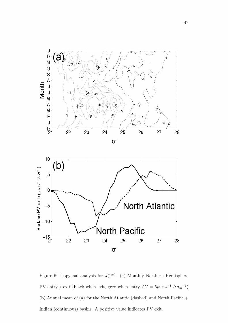
3.3 Isopycnal analysis

An alternative way to discuss the PV entry / exit at the sea surface is to

consider how it affects isopycnal layers, rather than geographical locations

(section 2.2 and “the impermeability theorem”). We have indicated in Figs.

3 and 4 the annual mean position of some selected isopycnal outcrops (thin

black lines). The latter actually move significantly meridionally and zonally

throughout the year (Fig. 5) so that a proper isopycnal analysis must track

14

the outcrop lines through their seasonal migration. We have thus followed

a range of isopycnal layers (density [σm, σm + ∆σm] with ∆σm = 0.2kgm−3)

and display in Fig. 6a how much PV enters / leaves each layer per unit time,

i.e., we plot

∆Jmechs (σm, t) =1

∆σm

∫ σm+∆σm

σm

Jmechs (x, y, t)dxdy (13)

in which t is a given calendar month. Strikingly, only a weak seasonal cycle is

seen, most isopycnals experiencing PV exchange of only one sign throughout

the year. The σm ' 24.5kgm−3 separates those isopycnal layers experiencing

PV entry (lighter isopycnals) from those experiencing PV exit (denser isopy-

cnals). This reflects the belt of surface westerlies poleward of the average

position of the ' 24.5kgm−3, destratifying the surface by advecting dense

water equatorward, and, conversely, Trade winds equatorward of this isopy-

cnal layer outcrop, stratifying the surface by advecting light water poleward

(Fig. 1). Note that this simple dipolar pattern masks a significant com-

pensation between PV entry and exit for light (low latitudes) isopycnals, as

hinted at in Fig. 3 (e.g., the annual mean outcrop of σm = 22 –thin black

line– experiences both PV entry and exit).

We display the annual mean of ∆Jmechs for the North Pacific (continuous)

and North Atlantic (dashed) basins 1 separately in Fig. 6b. As expected

from the higher surface density in the North Atlantic, the dipolar curve is

shifted towards the right in the North Atlantic compared to the North Pacific

1The ‘North Pacific’ calculation also includes the Northern Indian ocean.

15

by about 1kg m−3. Larger PV exit and entry is seen in the Pacific as a result

of the larger size of this basin.

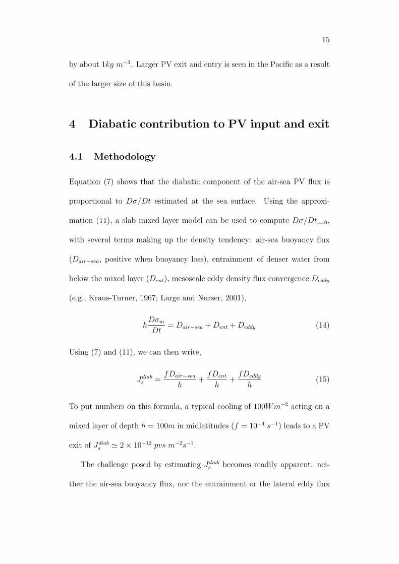
4 Diabatic contribution to PV input and exit

4.1 Methodology

Equation (7) shows that the diabatic component of the air-sea PV flux is

proportional to Dσ/Dt estimated at the sea surface. Using the approxi-

mation (11), a slab mixed layer model can be used to compute Dσ/Dtz=0,

with several terms making up the density tendency: air-sea buoyancy flux

(Dair−sea, positive when buoyancy loss), entrainment of denser water from

below the mixed layer (Dent), mesoscale eddy density flux convergence Deddy

(e.g., Kraus-Turner, 1967; Large and Nurser, 2001),

hDσmDt

= Dair−sea +Dent +Deddy (14)

Using (7) and (11), we can then write,

Jdiabs =fDair−sea

h+fDent

h+fDeddy

h(15)

To put numbers on this formula, a typical cooling of 100Wm−2 acting on a

mixed layer of depth h = 100m in midlatitudes (f = 10−4 s−1) leads to a PV

exit of Jdiabs ' 2× 10−12 pvs m−2s−1.

The challenge posed by estimating Jdiabs becomes readily apparent: nei-

ther the air-sea buoyancy flux, nor the entrainment or the lateral eddy flux

16

contribution to the buoyancy budget are known precisely from observations.

We have nevertheless constructed a tentative estimate of the first two terms

in (15), with no attempts at estimating the impact of the eddies, i.e., we will

use

Jdiabs ' fDair−sea

h︸ ︷︷ ︸J

(diab,ao)s

+fDent

h︸ ︷︷ ︸J

(diab,ent)s

(16)

The contribution J(diab,ao)s from the air-sea buoyancy flux was estimated using

the same mixed layer depth climatology as in section 3, plus a climatology of

air-sea density flux developed recently at Imperial College (Howe and Czaja,

2008). The latter’s thermal component is the adjusted climatology of Grist

and Josey (2003) while, for the haline part, the evaporation from Grist and

Josey (2003) and the precipitation from Xie and Arkin (1997) are used. Note

that both the haline and thermal components are constrained to satisfy the

global heat and freshwater budget obtained during WOCE (Ganachaud and

Wunsch, 2001). We refer to the paper by Howe and Czaja (2008) for more

discussion of this dataset.

The contribution J(diab,ent)s is more problematic and we have simply aimed

at giving a bound on the effects of entrainments. To get some insight into the

latter, consider the following “thought-experiment”. Consider an hypothet-

ical ocean only subject to spatially uniform, seasonally varying, buoyancy

forcing. Assume further that the net surface buoyancy flux is zero, with win-

tertime buoyancy loss balancing exactly summertime buoyancy gain, and let

us consider the simplest case of uniform rotation (f = constant). Because of

17

the seasonal correlation between Dair−sea and h (summertime air-sea buoy-

ancy gain when the mixed layer is shallow, buoyancy loss when the mixed

layer is deep), there will be a net annual gain of PV by the ocean. This is

problematic because, in this thought-experiment, there is no oceanic circula-

tion to transport PV to lateral boundaries where a frictional PV flux could

balance the surface PV input (or to a region of surface PV loss, if it was

present). The reason is simple: in wintertime, cooling of the mixed layer

occurs not only at the sea surface but also at the mixed layer base through

entrainment of cold water from below. This additional cooling mechanism

will, in this thought experiment, compensate exactly the larger summertime

PV gain caused by the shallowing of the mixed layer. As a way to estimate

this effect we have computed J(diab,ent)s using standard slab mixed layer model

results for Dent (e.g., Kraus and Turner, 1967),

Dent = went(σent − σm) (17)

in which σent is the density of water that is entrained into the mixed layer

and went is the entrainment velocity,

went =

0 when ∂h

∂t≤ 0

∂h/∂t when ∂h∂t> 0

(18)

Note that equation (18) omits the contribution to entrainment resulting from

convergence / divergence of the flow, but it allows for a simple calculation

using the mixed layer depth climatology mentionned above. The density

18

difference appearing in (17), namely,

∆entσ ≡ σent − σm (19)

is taken as a constant parameter. In their attempt at estimating the effects

of entrainment on transformation rates, Garrett and Tandon (1997) typically

used a value of ∆entb = 10−3 ms−2 for the buoyancy jump at the base of the

mixed layer, i.e., ∆entσ = ρo∆entb/g ' 0.1 kgm−3. Considering that our

estimate of went is certainly underestimated by the use of a smooth monthly

climatology of mixed layer depth, we have opted for investigating a range of

values 0 ≤ ∆entσ ≤ 0.5 kgm−3.

4.2 Northern Hemisphere maps

The annual mean value of Jdiabs computed with a value ∆entσ = 0.5 kgm−3 is

plotted for the Northern Hemisphere in Fig. 7, in a format analog to Fig. 3.

PV exit (dark shading) over the Gulf Stream and the Kuroshio is pronounced,

reflecting the large wintertime buoyancy loss over these regions. PV exit is

also found on the eastern side of Atlantic and Pacific subtropical basins,

reflecting the large surface evaporation maintained by the slow descent of

dry air over the oceans in the subsidence branch of the Hadley - Walker

circulations. At high latitudes, PV exit is found over the subpolar North

Atlantic but not over the subpolar North Pacific, which experiences PV entry.

The result of a calculation in which entrainment effects are not considered

(∆entσ = 0) is shown in Fig. 8a. Compared to Fig. 7, regions of PV exit

19

become less extensive, disappearing almost entirely in the subpolar North

Atlantic. This is consistent with the above ‘thought-experiment’, the seasonal

correlation between Dair−sea and h biasing J(diab,ao)s towards its summertime

value, when heating of the ocean leads to PV entry. To emphasize this point,

we have repeated the calculation in Fig. 8a using annual mean mixed layer

depth, rather than seasonal values (Fig. 8b). PV exit is then found over

most of the North Atlantic and North Pacific, the maps simply reflecting the

annual mean value of Dair−sea.

The fact that the subpolar North Pacific experiences diabatic PV en-

try results from the net surface buoyancy gain of this basin, itself reflecting

the weak surface evaporation associated with cold North Pacific sea surface

temperature (e.g., Warren, 1983). Very large entrainment effects would be

required to bring Jdiabs to zero (this happens when ∆entσ > 1.25 kgm−3),

which seems unrealistic. It is of course possible that the surface buoyancy

gain is overestimated over the subpolar gyre, so that the numbers are overall

uncertain (note however that, as discussed in Howe and Czaja (2008), our

Dair−sea dataset is in good agreement with others over this region). Nev-

ertheless, Figs. 7 and 3 highlight a very interesting qualitative difference

between North Atlantic and Pacific subpolar basins. In the North Atlantic,

both mechanical and diabatic contributions set a pattern of surface PV exit.

In the North Pacific, however, mechanical and diabatic effects oppose each

other with the winds driving PV exit but diabatic effects PV entry.

20

4.3 Isopycnal analysis

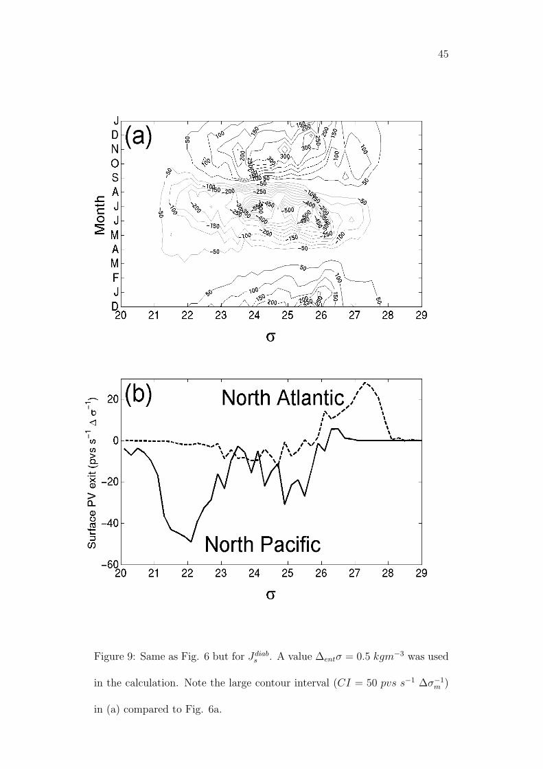
Figure 9a displays the seasonal evolution of the diabatic component of PV

entry/exit computed using a value ∆entσ = 0.5 kgm−3, for the same isopycnal

layers as in section 3, i.e. a plot of,

∆Jdiabs (σm, t) =1

∆σm

∫ σm+∆σm

σm

(J (diab,ao)s + J (diab,ent)

s )dxdy (20)

as a function of calendar months and isopycnal layers. The striking difference

with ∆Jmechs (Fig. 6a) is the strong seasonal cycle. In winter, surface cooling

leads to PV exit but the reverse occurs in summer, despite the isopycnal

layers typically moving poleward at that time of year (Fig. 5). Thus, rather

than experiencing solely PV input or exit throughout the year (as Jmechs

does), diabatic effects drive alternate, seasonally changing, PV entry/exit in

isopycnal layers. The summertime PV input is expected from the high values

of PV observed in oceanic seasonal thermoclines (e.g., Talley, 1988; Csanady

and Vittal, 1996). Conversely, wintertime surface PV exit is consistent with

the presence of low PV in deep mixed layers (Talley and Mc Cartney, 1982;

Thomas, 2005).

Comparison of Fig. 6a and 9a suggests that, on a given month, PV en-

try/exit is dominated by the diabatic contribution (note the larger contour

interval in Fig. 9a compared to Fig. 6a). Owing to the strong cancellation

between summer and winter, however, the annual mean of ∆Jdiabs is compa-

rable, although still larger on average, than that for ∆Jmechs (Fig. 9b). The

North Atlantic (dashed) displays PV exit over almost all isopycnal layers

21

while the North Pacific shows a more complicated structure. PV input is

found over σm ' 25, corresponding to isopycnals whose mean outcrop posi-

tion is in the subpolar gyre (Fig. 7, thin black line labelled 25), but is even

larger over the light isopycnals making the rim of the Indo-Pacific ‘warm

pool’ (σm ' 22). PV exit is only hinted at for the densest layers outcropping

in winter (σm > 26 –see Fig. 5).

5 Net surface PV entry / exit

5.1 Northern Hemisphere maps

The net PV entry/exit at the sea surface is estimated as

Js = Jdiab,aos + Jdiab,ents + Jmechs (21)

and its annual mean distribution is shown in Fig. 10, in a format similar

to Fig. 3. A value ∆entσ = 0.5 kgm−3 was used, so that the estimate in

Fig. 10 is the sum of those shown in Fig. 3 and Fig. 7. To gain some

confidence in the pattern, we compare it to Marshall et al. (2001)’s Fig. 4c,

which shows, for the North Atlantic only, an ocean model estimate of Js.

The comparison is very good, both in sign and amplitude (the comparison

obviously depends upon the choice of ∆entσ and we have not attempted to

optimize this parameter to improve the comparison with Marshall et al’s

map). The North Atlantic shows a quadrupolar pattern of air-sea PV flux,

with PV gain at low latitudes, PV loss in the eastern subtropics and over

22

the Florida current, PV gain south of the separated Gulf Stream and over

the Labrador current, and PV loss along the Gulf Stream and over most of

the subpolar gyre. The strongest PV loss is found over the Gulf Stream,

with values larger than 10.1012 pvs m−2 s−1 (see scalings in sections 3 and

4). Considering the uncertainties in the observational datasets needed to

estimate Js, and the simplicity of our model for entraiment, the comparison

is very encouraging.

The Northern Hemisphere map (Fig. 10) as a whole shows striking dif-

ferences between the Atlantic and Pacific. In the extra-tropics, the tongue

of PV exit over the western boundary current is limited to about 40N and

mid-basin (' 180W ) in the North Pacific wheareas it extends all the way

to the high latitudes in the North Atlantic. Put differently, the net subpolar

PV entry, which is limited to the Labrador current area in the Atlantic, is

seen to occupy the whole subpolar gyre in the North Pacific. The opposition

between mechanical and diabatic effects in the North Pacific, but their con-

structive association in the North Atlantic (see section 4), is clearly key to

establishing this contrast between the basins.

5.2 Isopycnal analysis

Figure 10 suggests that isopycnals outcropping frequently over the North

Pacific subpolar gyre should experience net PV entry. To check this we

turn to a proper isopycnal analysis for Js and first identify the isopycnals

23

layers experiencing Ekman downwelling (hereafter “subtropical isopycnals”)

or upwelling (hereafter “subpolar isopycnals”) in the annual mean (Fig. 11

-for this purpose the same monthly windstress climatology was used as in

section 3). In the North Atlantic (dashed line), isopycnals denser than σm '

27) experience Ekman suction (Ekman velocity wEk > 0) while those lighter,

pumping (wEk < 0). The situation in the North Pacific (continuous line)

is a bit more complicated, with suction at σm > 25.5 and σm < 21.75 and

pumping in between.

Next we display in Fig. 12 the result of a calculation similar to Figs. 4b,

9b but for Js rather than Jmechs and Jdiabs . In the North Pacific (continuous

curve) a more intuitive PV exit rather than input at high density (σm >

26) is now found, reflecting the fact that the densest “subpolar isopycnals”

only outcrop at the sea surface in winter, when the mixed layer experiences

buoyancy loss. The high latitude net PV input, so prominent in Fig. 10, is

still seen over the intermediate density range σm ' 24−26, but inspection of

Fig. 11 shows that the maximum PV entry at σm ' 25.5 in Fig. 12 coincides

with the subtropical / subpolar gyre boundary. Thus, the ‘fixed location

analysis’ (Fig. 10) somewhat distorts the isopycnal view (only light subpolar

gyre isopycnals experience net PV entry in the North Pacific). Additional

analysis of the role of heating and freshening in providing the buoyancy gain

for those ‘inter-gyre isopycnals’ indicate the freshening to be dominant (not

shown). This result is consistent with the presence of net precipitation at the

24

boundary between the gyres in the North Pacific as a result of the Summer

Asian Monsoon (Czaja, 2008 –see his Fig. 3b).

A similar isopycnal analysis for the North Atlantic (Fig. 12, dashed curve)

reveals a much simpler dipolar picture, with net PV exit for isopycnals denser

than σm ' 25 and net PV entry for isopycnals lighter than σm ' 25. In other

words, unlike in the North Pacific, there is no indication of an ‘intermediate

’ (at the boundary between subpolar and subtropical gyres) isopycnal range

experiencing net PV entry. Net PV exit is associated, on the lighter end

(σm ' 25 − 27), with isopycnals outcropping in the subtropics in regions of

Ekman downwelling, and experiencing PV loss associated with large scale

subtropical evaporation and air-sea interactions over the Gulf Stream. On

the denser end (σm > 27), net PV exit is associated with high latitude cooling

and Ekman upwelling. Net PV input is solely confined to regions of Ekman

downwelling. The broad peak in net PV exit at σm ' 26 − 27 is consistent

with Marshall et al. (2001)’s isopycnal analysis for the North Atlantic (their

Fig. 8), but their model study suggests net PV exit for all density classes,

not solely for σm ≥ 25 as found here.

6 Discussion

The estimates of surface PV entry / exit presented in this study must be taken

with caution considering the large number of datasets which are needed to

construct them: surface windstress, mixed layer depth and density, net sur-

25

face buoyancy and entrainment fluxes. It is hard to argue that the latter are

known accurately and so are, consequently, our PV flux maps. A possible al-

ternative, which we tried, is to use Schar (1993)’s formulation of the J-vector,

which only requires knowledge of mixed layer density and surface pressure 2

–see section 2.2. In practise however, this method turned out to be difficult

to use. Indeed, to obtain a global seasonal climatology of surface pressure,

we used the sea surface height measurements from the Topex-Poseidon / Ja-

son altimeters. Owing to errors on the geoid at the gridpoint scale (2× 2),

residual oceanic variability (a 12-yr mean was used which is short for proper

ocean statistics) and errors on the hydrography (seasonal cycle of mixed layer

density), the calculation turned out to be very noisy (and this in addition to

the fact that Schar’s formula itself is noisy by nature, since it is the advec-

tion of density by the geostrophic flow, i.e. a cross product of two gradient

vectors).

Our assumptions for the distribution of turbulent fluxes in the mixed

layer and our model for entrainment are admittedly crude. They do not take

into account mixed layer entrainment of momentum, or the high frequency

(synoptic) storm variability, or spatial variability of the density jump at the

base of the mixed layer (∆entσ). We found however our main conclusions

to be unchanged when varying ∆entσ. The North Atlantic systematically

2At the sea surface, Schaar’s expression reads Js = (∇gη ×∇σm).k in which we have

approximated the Bernoulli function by the surface geopotential height (B = 12 |~u|

2 +

p/ρo ' p/ρo = gη, g being gravity and η the height of the sea surface).

26

displays net PV exit at high density and net PV entry at lower density, the

value of ∆entσ solely changing the density at which the transition occurs and

the overall magnitude of the PV exit / entry. In the North Pacific, a value

∆entσ ' 1 kgm−3 is needed to remove the net PV entry in intermediate

density class seen in Fig. 12 (σm = 24− 26), which seems unrealistic.

Probably the most striking result of our analysis is the difference between

the distribution of PV entry / exit for the high latitude North Atlantic and

Pacific. Because of the large poleward flow of warm waters associated with

the thermohaline circulation in the Atlantic, there is a strong surface evapo-

rative cooling at high latitudes which acts to remove PV at the sea surface.

The westerlies add constructively to this, resulting, overall, in a net PV exit

along the path of the North Atlantic Drift (Fig. 10) or isopycnal layers denser

than σm ≥ 26 (Fig. 12). In the subpolar gyre of the North Pacific, however,

no such poleward circulation is found in upper layers and there is net surface

buoyancy gain at high latitudes. Diabatic effects thus tend to restratify the

surface (PV entry) and oppose the effect of the westerlies (PV exit) in the

North Pacific. Our analysis suggests that, in total, diabatic effects dominate,

with a net PV entry over the subpolar gyre (Fig. 10). This view is some-

what distorted from that seen in the isopycnal analysis of Fig. 12 (the bulk

of the PV entry is experienced by ‘inter-gyre isopycnals’, the denser layers

experiencing PV exit –see section 5.2).

Considering the uncertainties discussed above in the calculation of Js,

27

it is difficult to claim with confidence that the North Pacific subpolar gyre

experiences net surface PV entry. The compensation between diabatic and

mechanical effects is appealing and might indeed lead to a neutral distribution

of PV entry / exit for this region, i.e., Js ' 0. Non eddying models of the

subpolar gyre show indeed a scenario whereby, in the interior, advective PV

transport balances frictional PV transport, thereby having no difficulty at

dealing with a zero sea surface PV exit (Marshall, 2000). Alternatively,

eddies acting downgradient on large isopycnic gradients of PV in the spring

/ early summer (e.g., Talley, 1985) could be instrumental in transporting into

the oceanic interior the PV that enters through the sea surface, dominating

over the upward mean PV transport by the Sverdrup flow (Fig. 13a). This

is in sharp contrast with the dynamics suggested in the North Atlantic, in

which a clear net PV exit is found at the sea surface, connecting to the

mean upward PV transport by the Gulf Stream and the North Atlantic Drift

(“thermohaline circulation”) in the interior (Fig. 13b).

Some support for this view of the North Pacific is provided by the ob-

served Tritium distribution (Fine et al., 1981). Indeed, considering that all

the PV transport below the mixed layer is advective, a southward PV trans-

port as in Fig. 13a should relate to a southward tracer transport. Fine et al.

(1981) consistently show a significant southward spreading of high Tritium

value towards the South for isopycnals outcropping in winter in the subpolar

gyre (σθ = 26.02, their Fig. 6). We note further that the state of affair de-

28

picted in Fig. 13a for the North Pacific is reminiscent of the dynamics at high

latitudes of the Southern Ocean. There, downgradient eddy PV fluxes along

isopycnal surfaces (i.e., downward and equatorward PV transport) have been

suggested to drive the lower branch of the Deacon cell (Speer et al., 2000).

7 Conclusion

We have presented, for the first time, an observational estimate of PV en-

try/exit at the sea surface. The North Atlantic appears as a ‘textbook’

example of surface PV exit in the western boundary current extension / sub-

polar gyre and surface PV entry over most parts of the subtropical gyre,

but investigation of the mechanisms setting this pattern highlight the com-

plementary role of diabatic and mechanical processes. The North Pacific

displays a more complicated pattern of PV entry / exit. Our main results

can be summarized as follows:

• Air-sea buoyancy fluxes drive seasonally varying PV entry/exit on isopy-

cnal layers whereas the winds do not.

• Western boundary currents and their interior extension experience net

surface PV exit.

• Subtropical gyres experience both PV entry and exit, with similar pat-

terns in the Atlantic and Pacific.

• The subpolar gyres of the North Pacific and Atlantic differ strikingly

29

in their surface distribution of PV exit and entry. This reflects the

constructive effect of mechanical and diabatic effects in the North At-

lantic, leading to a clear net PV exit along the path of the North

Atlantic current, but their opposition in the North Pacific, leading to

a more uncertain (possibly net entry) surface PV flux.

Our study illustrates the fundamentally coupled (ocean-atmosphere) nature

of the entry and exit of PV at the sea surface. This is vividly illustrated

in the tropical Pacific, where coupled air-sea interactions displace the ITCZ

and its belt of warm water north of the equator, setting reversals in the

meridional density gradient and surface PV exit equatorward of the ITCZ

but PV entry on the poleward side of the ITCZ . Conversely, the presence

of an active thermohaline cell in the Atlantic, leading to warmer sea surface

temperature and evaporation at high latitudes in this basin compared to

the North Pacific, is vividly ‘seen’ in the extension to high latitudes of the

western boundary tongue of surface PV exit.

Clearly though, considering the large number of observational datasets

needed to produce the air-sea PV flux, and the imperfections associated

with them, further work with oceanic reanalyses, ocean-only GCMs or cou-

pled ocean-atmosphere GCMs is needed to test the reproducibility of our

results. It will be fascinating to match the surface PV entry / exit presented

in this study with interior transport using eddy resolving GCM simulations.

30

References

Csanady, G. T., and G. Vittal, 1996: Vorticity balance of outcropping isopy-

cnals, J. Phys. Oce., 26, 1952-1956.

Czaja, A, 2008: Atmospheric control on the thermohaline circulation, J.

Phys. Oce., in press.

Fine, R. A., J. L. reid, H. G. Ostlund, 1981: Circulation of Tritium in the

Pacific Ocean, J. Phys. Oce., 11, 3-14.

Ganachaud, A. and C. Wunsch, 2003: Large-scale ocean heat and freshwater

transports during the World Ocean Circulation Experiment, J. Clim., 16,

696-705.

Garrett, C., and A. Tandon, 1997: The effects on water mass formation of

surface mixed layer time dependence and entrainment fluxes, Deep-Sea Res.,

44, No 12, 1991-2006.

Gill, A. E. J., 1982: Atmosphere - Ocean Dynamics, Academic press.

Grist, J. P., and S. A. Josey, 2003: Inverse analysis adjustment of the SOC

air-sea flux climatology using ocean heat transport constraints, J. Clim., 16,

3274-3295.

Haynes, P. H., and M. E. McIntyre, 1987: On the evolution of vorticity and

potential vorticity in the presence of diabatic heating and frictional or other

forces, J. Atm. Sci., 44, 5, 828-841.

31

Haynes, P. H., and M. E. McIntyre, 1990: On the conservation and imper-

meability theorems for potential vorticity, J. Atm. Sci., 47, 16, 2021-2031.

Hoskins, B. J., 1991: Towards a PV-θ view of the general circulation, Tellus,

43AB, 27-35.

Howe, N. and A. Czaja, 2008: A globally balanced air-sea density flux clima-

tology and global surface transformation rates, submitted to J. Phys. Oce.

Keffer, T., 1985: The ventilation of the world’s oceans: maps of the potential

vorticity field, J. Phys. Oce., 15, 509-523.

King, C., D. Stammer, and C. Wunsch, 1994: The CMPO/MIT

Topex/Poseidon Altimetric data set, M.I.T, Centre for Global Change Sci-

ence, Report No 30.

Kraus, E. B., and J. S. Turner, 1967. A one - dimensional model of the

seasonal thermocline, II, Tellus, 19, 98-106.

Large, W. G., and A. J. G. Nurser, 2001: Ocean surface water mass trans-

formation, Chap. 5.1 in ‘Ocean Circulation and Climate’, Academic Press,

715pp.

Luyten, J. R., J. Pedlosky and H. Stommel, 1983: The ventilated thermo-

cline, J. Phys. Oce., 13, 292-309.

Marshall, D. P., 2000: Vertical fluxes of potential vorticity and the structure

of thermocline, J. Phys. Oce., 30, 3102-3112.

32

Marshall, J. C., 1984: Eddy-mean flow interaction in a barotropic ocean

model, Q. J. Roy. Met. Soc., 110, 573-590.

Marshall, J. C., and A. J. G. Nurser, 1992: Fluid dynamics of oceanic ther-

mocline ventilation, J. Phys. Oce., 22, 583-595.

Marshall, J., A. J. G. Nurser, and R. G. Williams, 1993: Inferring the subduc-

tion rate and period over theh North Atlantic, J. Phys. Oce., 23, 1315-1329.

Marshall, J. C., D. Jamous, and J. Nilsson, 2001: Entry, flux, and exit of

potential vorticity in ocean circulation, J. Phys. Oce., 31, 777-789.

McDowell, S., P. Rhines, and T. Keffer, 1982: North Atlantic potential vor-

ticity and its relation to the general circulation, J. Phys. Oce., 12, 1417-1436.

O’Dwyer, J., and R. G. Williams, 1997: The climatological distribution of

potential vorticity over the abyssal ocean, J. Phys. Oce., 27, 2488-2506.

Pedlosky, J., 1998. Ocean Circulation Theory, Springer, 453pp.

Rhines, P. B. 1993: Oceanic general circulation: wave and advection dynam-

ics, NATO ASI series vol I 11, Modelling Oceanic Climate Interactions, D.

Anderson and J. Willebrandt, eds.

Rhines, P. B. and W. R. Young, 1982: A theory of the wind driven circulation.

I. Mid-ocean gyres, J. Mar. Res., 40, 559-596.

Schar, C., 1993: A generalisation of Bernoulli’s theorem, J. Atm. Sci., 50,

1437-1443.

33

Schmitz, W. J., 1996. On the world ocean circulation: Vol II, The Pacific

nd indian Oceans / a global update, Woods Hole Oceanographic Institution,

Technical Report, WHOI-96-08.

Speer, K., S. R. Rintoul, and B. Sloyan, 2000: The diabatic Deacon cell, J.

Phys. Oce., 3212-3222.

Talley, L. D., 1988: Potential vorticity distribution in the North Pacific, J.

Phys. Oce., 18, 89-106.

Talley, L. D. and M. S. McCartney, 1982: Distribution and circulation of

Labrador sea water, J. Phys. Oce., 12, 1189-1205.

Thomas, L., 2005: Destruction of potential vorticity by winds, J. Phys. Oce.,

35, 2457-2466.

Warren B. A., 1983: Why is no deep water formed in the North Pacific?, J.

Mar. Res., 41, 327-347.

Xie, P. P. and P. A. Arkin, 1996: Analyses of global monthly precipitation us-

ing gauge observations, satellite estimates, and numerical model predictions,

J. Clim., 9, 840-858.

34

List of Figures

1 Schematic of the PV exit (entry) at an outcropping isopycnal

surface associated with a surface westerly (easterly) stress and

surface buoyancy loss (gain), assuming a simple equator-to-

pole gradient of surface density. The PV flux (upward for PV

exit, Js > 0) is schematized as the white arrow. . . . . . . . . 37

2 A “thought-experiment” to illustrate the difference between

the transfer of heat (left side, as indicated by the grey arrow)

and PV (right side, black arrows). The initial potential tem-

perature distributions are indicated by the continuous black

lines while the dashed line defines the equilibrium temperature

θeq. See text for details. . . . . . . . . . . . . . . . . . . . . . 38

3 Annual mean mechanical contribution (Jmechs ) to the sea sur-

face PV entry/exit (shading, dark when out of the ocean, light

when into the ocean, in units of 10−12pvs s−1m−2, zero con-

tour as black thick line) superimposed on annual mean mixed

layer density (contoured every 1 kgm−3 in thin black lines). . . 39

4 Same as Fig. 3 but by simplifying (12) as (a) τx(∂σm/∂y)/ρoh

and (b) τx(∂σm/∂y)ref/ρoh in wich (∂σm/∂y)ref = 1kgm−3/1000km. 40

5 Location of selected mixed layer isopycnal outcrops for March

(black) and September (grey). (a) σm = 27 (b) σm = 26 (c)

σm = 24 (d) σm = 22. . . . . . . . . . . . . . . . . . . . . . . . 41

35

6 Isopycnal analysis for Jmechs . (a) Monthly Northern Hemi-

sphere PV entry / exit (black when exit, grey when entry,

CI = 5pvs s−1 ∆σm−1) (b) Annual mean of (a) for the North

Atlantic (dashed) and North Pacific + Indian (continuous)

basins. A positive value indicates PV exit. . . . . . . . . . . . 42

7 Same as Fig. 3 but for the annual mean diabatic contribution

Jdiabs (air-sea buoyancy flux + entrainment) to the sea sur-

face PV entry/exit. A value ∆entσ = 0.5 kgm−3 was used to

produce this map. . . . . . . . . . . . . . . . . . . . . . . . . . 43

8 Same as Fig. 7 but with ∆entσ = 0 (a) with the seasonal cycle

in mixed layer depth (b) without seasonal cycle in mixed layer

depth (i.e., h set to its annual mean value). . . . . . . . . . . . 44

9 Same as Fig. 6 but for Jdiabs . A value ∆entσ = 0.5 kgm−3

was used in the calculation. Note the large contour interval

(CI = 50 pvs s−1 ∆σ−1m ) in (a) compared to Fig. 6a. . . . . . . 45

10 Same as Fig. 3 but for the net PV entry / exit at the sea surface. 46

11 Integrated Ekman pumping wEk over isopycnal layers of width

∆σ = 0.2kg m−3, in units of Sv∆σ−1 (1Sv = 106m3s−1). . . . 47

12 Same as Fig. 6b but for the net PV entry / exit at the sea

surface. . . . . . . . . . . . . . . . . . . . . . . . . . . . . . . 48

36

13 A schematic of PV transport along a subpolar gyre isopycnal

in the North (a) Pacific (b) Atlantic. The entry / exit of

PV at the sea surface is indicated by a white arrow, while

the advective transport of PV by the mean Sverdrup flow is

depicted by a straight black arrow. Wiggly black arrows depict

the advective transport of PV due to eddy motions. . . . . . . 49

37

Figure 1: Schematic of the PV exit (entry) at an outcropping isopycnal sur-

face associated with a surface westerly (easterly) stress and surface buoyancy

loss (gain), assuming a simple equator-to-pole gradient of surface density.

The PV flux (upward for PV exit, Js > 0) is schematized as the white arrow.

38

Figure 2: A “thought-experiment” to illustrate the difference between the

transfer of heat (left side, as indicated by the grey arrow) and PV (right side,

black arrows). The initial potential temperature distributions are indicated

by the continuous black lines while the dashed line defines the equilibrium

temperature θeq. See text for details.

39

Figure 3: Annual mean mechanical contribution (Jmechs ) to the sea surface PV

entry/exit (shading, dark when out of the ocean, light when into the ocean,

in units of 10−12pvs s−1m−2, zero contour as black thick line) superimposed

on annual mean mixed layer density (contoured every 1 kgm−3 in thin black

lines).

40

Figure 4: Same as Fig. 3 but by simplifying (12) as (a) τx(∂σm/∂y)/ρoh and

(b) τx(∂σm/∂y)ref/ρoh in wich (∂σm/∂y)ref = 1kgm−3/1000km.

41

Figure 5: Location of selected mixed layer isopycnal outcrops for March

(black) and September (grey). (a) σm = 27 (b) σm = 26 (c) σm = 24 (d)

σm = 22.

42

Figure 6: Isopycnal analysis for Jmechs . (a) Monthly Northern Hemisphere

PV entry / exit (black when exit, grey when entry, CI = 5pvs s−1 ∆σm−1)

(b) Annual mean of (a) for the North Atlantic (dashed) and North Pacific +

Indian (continuous) basins. A positive value indicates PV exit.

43

Figure 7: Same as Fig. 3 but for the annual mean diabatic contribution Jdiabs

(air-sea buoyancy flux + entrainment) to the sea surface PV entry/exit. A

value ∆entσ = 0.5 kgm−3 was used to produce this map.

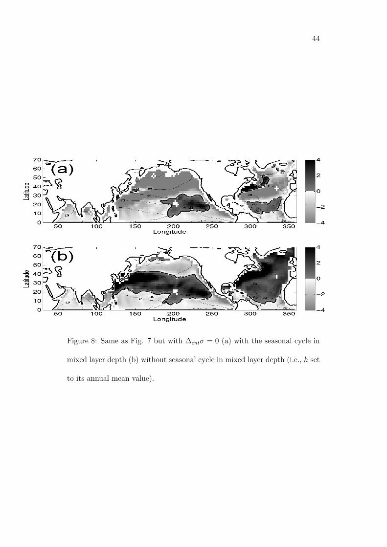
44

Figure 8: Same as Fig. 7 but with ∆entσ = 0 (a) with the seasonal cycle in

mixed layer depth (b) without seasonal cycle in mixed layer depth (i.e., h set

to its annual mean value).

45

Figure 9: Same as Fig. 6 but for Jdiabs . A value ∆entσ = 0.5 kgm−3 was used

in the calculation. Note the large contour interval (CI = 50 pvs s−1 ∆σ−1m )

in (a) compared to Fig. 6a.

46

Figure 10: Same as Fig. 3 but for the net PV entry / exit at the sea surface.

47

Figure 11: Integrated Ekman pumping wEk over isopycnal layers of width

∆σ = 0.2kg m−3, in units of Sv∆σ−1 (1Sv = 106m3s−1).

48

Figure 12: Same as Fig. 6b but for the net PV entry / exit at the sea surface.

49

Figure 13: A schematic of PV transport along a subpolar gyre isopycnal in

the North (a) Pacific (b) Atlantic. The entry / exit of PV at the sea surface is

indicated by a white arrow, while the advective transport of PV by the mean

Sverdrup flow is depicted by a straight black arrow. Wiggly black arrows

depict the advective transport of PV due to eddy motions.