Observational Probes of Cosmic Acceleration

David H. Weinberga,b,c, Michael Mortonsonb, Daniel J. Eisensteind,e, Christopher Hirataf, AdamRiessg, Eduardo Rozoh

aDepartment of Astronomy, Ohio State University, Columbus, OH 43210bCenter for Cosmology and Astro-Particle Physics, Ohio State University, Columbus, OH 43210

cInstitute for Advanced Study, Princeton, NJ 08540dSteward Observatory, University of Arizona, Tucson, AZ

eHarvard College Observatory, 60 Garden St., Cambridge, MA 02138fCalifornia Institute of Technology, Pasadena, CA

gDepartment of Physics and Astronomy, Johns Hopkins University, Baltimore, MD 21218hKavli Institute for Cosmological Physics, University of Chicago, Chicago, IL 60637

Abstract

This is a partial draft of a review article in preparation for Physics Reports, provided to membersof the WFIRST Science Definition Team for reference. We have included only those sections thatare close to complete. However, even these sections are still subject to change, so we request thatthis draft not be circulated beyond the SDT. We plan to solicit comments on the full manuscriptbefore it is submitted to the journal.

Keywords:

1. Introduction

Gravity pulls. Newton’s Principia generalized this longstanding fact of human experience into auniversal attractive force, providing compelling explanations of an extraordinary range of terrestrialand celestial phenomena. Newtonian attraction weakens with distance, but it never vanishes, andit never changes sign. Einstein’s theory of General Relativity (GR) reproduces Newtonian gravityin the limit of weak spacetime curvature and low velocities. For a homogeneous universe filled withmatter or radiation, GR predicts that the cosmic expansion will slow down over time, in accord withNewtonian intuition. In the late 1990s, however, two independent studies of distant supernovaefound that the expansion of the universe has accelerated over the last five billion years (Riess et al.,1998; Perlmutter et al., 1999), a remarkable discovery that is now buttressed by multiple lines ofindependent evidence. On the scale of the cosmos, gravity repels.

Cosmic acceleration is the most profound puzzle in contemporary physics. Even the least exoticexplanations demand the existence of a pervasive new component of the universe with unusualphysical properties that lead to repulsive gravity. Alternatively, acceleration could be a sign thatGR itself breaks down on cosmological scales. Cosmic accleration may be the crucial empirical cluethat leads to understanding the interaction between gravity and the quantum vacuum, or revealsthe existence of extra spatial dimensions, or sheds light on the nature of quantum gravity itself.

Because of these profound implications, cosmic acceleration has inspired a wide range of am-bitious experimental efforts, which aim to measure the expansion history and growth of structurein the cosmos with percent-level precision or higher. In this article, we review the observationalmethods that underlie these efforts, with particular attention to techniques that are likely to seemajor advances over the next decade. We will emphasize the value of a balanced program that

Preprint submitted to Physics Reports February 3, 2011

pursues several of these methods in combination, both to cross-check systematic uncertainties andto take advantge of complementary information.

The remainder of this introduction briefly recaps the history of cosmic acceleration and currenttheories for its origin, then sets this article in the context of future experimental efforts and otherreviews of the field. Section 2 describes the basic observables that can be used to probe cosmicacceleration, relates them to the underlying equations that govern the expansion history and thegrowth of structure, and introduces some of the parameters commonly used to define “generic”cosmic acceleration models. It concludes with an overview of the leading methods for measuringthese observables. In Sections 3-6, we go through the four most well developed methods in detail:Type Ia supernovae, baryon acoustic oscillations (BAO), weak gravitational lensing, and clustersof galaxies. Section 7 summarizes several other potential probes, whose prospects are currentlymore difficult to assess. Informed by the discussions in these sections, §8 presents our principalnew results: forecasts of the constraints on cosmic acceleration models that could be achieved bycombining results from these methods, based on ambitious but feasible experiments like the onesendorsed by the Astro2010 Decadal Survey report, New Worlds, New Horizons in Astronomy and

Astrophysics. We summarize the implications of our analyses in §9.

1.1. History

Just two years after the completion of General Relativity, Einstein (1917) introduced the firstmodern cosmological model. With little observational guidance, Einstein assumed (correctly) thatthe universe is homogeneous on large scales, and he proposed a matter-filled space with finite,positively curved, 3-sphere geometry. He also assumed (incorrectly) that the universe is static.Finding these two assumptions to be incompatible, Einstein modified the GR field equation toinclude the infamous “cosmological term,” now usually known as the “cosmological constant” anddenoted Λ. In effect, he added a new component whose repulsive gravity could balance the attractivegravity of the matter (though he did not describe his modification in these terms). In the 1920s,Friedmann (?) and Lemaitre (?) introduced GR-based cosmological models with an expandingor contracting universe, some of them including a cosmological constant, others not. In 1929,Hubble discovered direct evidence for the expansion of the universe (Hubble, 1929), thus removingthe original motivation for the Λ term. In 1965, the discovery and interpretation of the cosmicmicrowave background (Penzias and Wilson, 1965; Dicke et al., 1965) provided the pivotal evidencefor a hot big bang origin of the cosmos.

From the 1930s through the 1980s, a cosmological constant seemed unnecessary to explainingcosmological observations. The “cosmological constant problem” as it was defined in the 1980swas a theoretical one: why was the gravitational impact of the quantum vacuum vanishingly smallcompared to the “naturally” expected value (see §1.2)? In the late 1980s and early 1990s, however,a variety of indirect evidence began to accumulate in favor of a cosmological constant. Studiesof large scale galaxy clustering, interpreted in the framework of cold dark matter models withinflationary initial conditions, implied a low matter density parameter Ωm = ρm/ρcrit ≈ 0.15 − 0.4(e.g., Maddox et al. 1990; Efstathiou et al. 1990), in agreement with direct dynamical estimatesthat assumed galaxies to be fair tracers of the mass distribution. Reconciling this result withthe standard inflationary cosmology prediction of a spatially flat universe (Guth, 1981) required anew energy component with density parameter 1 − Ωm. Open-universe inflation models were alsoconsidered, but explaining the homogeneity of the cosmic microwave background (CMB) in suchmodels required speculative appeals to quantum gravity effects (e.g., Bucher et al. 1995) ratherthan the semi-classical explanation of traditional inflation.

By the mid-1990s, many cosmological simulation studies included both open-CDM models andΛ-CDM models, along with Ωm = 1 models incorporating tilted inflationary spectra, non-standard

2

radiation components, or massive neutrino components (e.g., ?). Once normalized to the observedlevel of CMB anisotropies, the large-scale structure predictions of open and flat-Λ models differed atthe tens-of-percent level, with flat models generally yielding a more natural fit to the observations(e.g., Cole et al. 1997). Thus, the combination of CMB data, large-scale structure data, andinflationary theory led many cosmologists to consider models with a cosmological constant, andsome to declare it as the preferred solution (e.g., Efstathiou et al. 1990; Krauss and Turner 1995;Ostriker and Steinhardt 1995).

Enter the supernovae. In the mid-1990s, two teams set out to measure the cosmic decelerationrate, and thereby determine the matter density parameter Ωm, by discovering and monitoring high-redshift, Type Ia supernovae. The recognition that the peak luminosity of supernovae was tightlycorrelated with the shape of the light curve (Phillips, 1993; Riess et al., 1996) played a criticalrole in this strategy, reducing the intrinsic distance error per supernova to ∼ 10%. While the firstanalysis of a small sample indicated deceleration (Perlmutter et al., 1997), by 1999 the two teamshad converged on a remarkable result: when compared to local Type Ia supernovae, the supernovaeat z ≈ 0.5 were fainter than expected in a matter-dominated universe with Ωm ≈ 0.2 by about 0.2mag, or 20% (Riess et al., 1998; Perlmutter et al., 1999). Even an empty, freely expanding universewas inconsistent with the observations. Both teams interpreted their measurements as evidence foran accelerating universe with a cosmological constant, consistent with a flat universe (Ωtot = 1)having ΩΛ ≈ 0.7.

Why was the supernova evidence for cosmic acceleration accepted so quickly by the communityat large? First, the internal checks carried out by the two teams, and the agreement of their con-clusions despite independent observations and many differences of methodology, seemed to rule outmany forms of observational systematics, even relatively subtle effects of photometric calibrationor selection bias. Second, the ground had been well prepared by the CMB and large scale struc-ture data, which already provided substantial indirect evidence for a cosmological constant. Thisconfluence of arguments favored the cosmological interpretation of the results over astrophysicalexplanations such as evolution of the supernova population or grey dust extinction that increasedtowards higher redshifts. Third, the supernova results were followed within a year by the resultsof balloon-borne CMB experiments that mapped the first acoustic peak and measured its angularlocation, providing strong evidence for spatial flatness (de Bernardis et al. 2000; Hanany et al. 2000;see Netterfield et al. 1997 for earlier ground-based measurements hinting at the same result). On itsown, the acoustic peak only implied Ωtot ≈ 1, not a non-zero ΩΛ, but it dovetailed perfectly with theestimates of Ωm and ΩΛ from large scale structure and supernovae. Furthermore, the acoustic peakmeasurement implied that the alternative to Λ was not an open universe but a strongly decelerating,Ωm = 1 universe, which disagreed with the supernova data by 0.5 magnitudes, a level much harderto explain with observational or astrophysical effects. Finally, the combination of spatial flatnessand improving measurements of the Hubble constant (e.g., H0 = 71 ± 6 km s−1 Mpc−1; Mouldet al. 2000) provided an entirely independent argument for an energetically dominant acceleratingcomponent: a matter-dominated universe with Ωtot = 1 would have age t0 = (2/3)H−1

0 ≈ 9.5Gyr, too young to accommodate the 12-14 Gyr ages estimated for globular clusters (e.g., Chaboyer1998).

A decade later, the web of observational evidence for cosmic acceleration is intricate and robust.A wide range of observations, including larger and better calibrated supernova samples over a widerredshift range, high-precision CMB data down to small angular scales, the baryon acoustic scale ingalaxy clustering, weak lensing measurements of dark matter clustering, the abundance of massiveclusters in X-ray and optical surveys, the level of structure in the Lyα forest, and precise measure-ments of H0, are all consistent with an inflationary cold dark matter model with a cosmological

3

constant, commonly abbreviated as ΛCDM.1 Explaining all of these data simultaneously requires

an accelerating universe. Completely eliminating any one class of constraints (e.g., supernovae, orCMB, or H0) would not change this conclusion, nor would doubling the estimated systematic errorson all of them. The question is no longer whether the universe is accelerating, but why.

1.2. Theories of Cosmic Acceleration

A cosmological constant is the mathematically simplest solution to the cosmic accelerationpuzzle. While Einstein introduced his cosmological term as a modification to the curvature side ofthe field equation, it is now more common to interpret Λ as a new energy component, constant inspace and time. For an ideal fluid with energy density u and pressure p, the effective gravitationalsource term in GR is (u + 3p)/c2, reducing to the usual mass density ρ = u/c2 if the fluid isnon-relativistic. For a component whose energy density remains constant as the universe expands,the first law of thermodynamics implies that when a comoving volume element in the universeexpands by a (physical) amount dV , the corresponding change in energy is related to the pressurevia −pdV = dU = udV , making the gravitational source term −2u/c2. A form of energy that isconstant in space and time must have a repulsive gravitational effect.

According to quantum field theory, “empty” space is filled with a sea of virtual particles. Itwould be reasonable to interpret the cosmological constant as the gravitational signature of thisquantum vacuum energy, much as the Lamb shift is a signature of its electromagnetic effects.2

The problem is one of magnitude. Since virtual particles of any allowable mass can come intoexistence for short periods of time, the “natural” value for the quantum vacuum density is onePlanck Mass per cubic Planck Length. This density is about 120 orders of magnitude larger thanthe cosmological constant suggested by observations: it would drive accelerated expansion with atimescale of tPlanck ≈ 10−43 sec instead of tHubble ≈ 1018 sec. Since the only “natural” number closeto 10−120 is zero, it was generally assumed (prior to 1990) that a correct calculation of the quantumvacuum energy would eventually show it to be zero, or at least suppressed by an extremely largeexponential factor (see review by Weinberg 1989). But the discovery of cosmic acceleration raisesthe possibility that the quantum vacuum really does act as a cosmological constant, and that itsenergy scale is 10−3 eV rather than 1028 eV for reasons that we do not yet understand. To date,there are no compelling theoretical arguments that explain either why the fundamental quantumvacuum energy might have this magnitude or why it might be zero.

The other basic puzzle concerning a cosmological constant is: Why now? The ratio of a constantvacuum energy density to the matter density scales as a3(t), so it has changed by a factor of ∼ 1027

since big bang nucleosynthesis and by a factor ∼ 1042 since the electroweak symmetry breakingepoch, which seems (based on our current understanding of physics) like the last opportunity fora major rebalancing of matter and energy components. It therefore seems remarkably coincidentalfor the vacuum energy density and the matter energy density to have the same order of magnitudetoday. In the late 1970s, Robert Dicke used a similar line of reasoning to argue for a spatiallyflat universe (?), an argument that provided much of the initial motivation for inflationary theory(Guth, 1981). However, while the universe appears to be impressively close to spatial flatness, theexistence of two energy components with different a(t) scalings means that Dicke’s “coincidenceproblem” is still with us.

One possible solution to the coincidence problem is anthropic: if the vacuum energy assumeswidely different values in different regions of the universe, then conscious observers will find them-

1Many of the relevant observational references will appear in subsequent sections on specific topics.2This interpretation of the cosmological constant was first suggested in the late 1960s by ?; for further discussion

of the history see Peebles and Ratra (2003).

4

selves in regions of the universe where the vacuum energy is low enough to allow structure formation(Efstathiou, 1995; Martel et al., 1998). This type of explanation finds a natural home in “mul-tiverse” models of eternal inflation, where different histories of spontaneous symmetry breakinglead to different values of physical constants in each non-inflating “bubble” (Linde, 1987), and ithas gained new prominence in the context of string theory, which predicts a “landscape” of vacuaarising from different compactifications of spatial dimensions (Susskind, 2003). One can attemptto derive an expectation value of the observed cosmological constant from such arguments (e.g.,Martel et al. 1998), but the results are sensitive to the choice of parameters that are allowed tovary (Tegmark and Rees, 1998) and to the choice of measure on parameter space, so it is hard totake such “predictions” beyond a qualitative level. A variant on these ideas is that the effectivevalue (and perhaps even the sign) of the cosmological constant varies in time, and that structurewill form and observers arise during periods when its magnitude is anomalously low compared toits natural (presumably Planck-level) energy scale (?Griest, 2002).

A straightforward alternative to a cosmological constant is a field with negative pressure (andthus repulsive gravitational effect) whose energy density changes with time (Ratra and Peebles,1988). In particular, a canonical scalar field φ with potential V (φ) has energy density and pressure

uφ = 12

1~c3 φ2 + V (φ),

pφ = 12

1~c3

φ2 − V (φ), (1)

so if the kinetic term is subdominant, then pφ ≈ −uφ. A slowly rolling scalar field of this sort isanalogous to the inflaton field hypothesized to drive inflation, but at an energy scale many, manyorders of magnitude lower. In general, a scalar field has an equation-of-state parameter

w ≡ p

u(2)

that is greater than −1 and varies in time, while a true cosmological constant has w = −1 at alltimes. Some forms of V (φ) allow attractor or “tracker” solutions in which the late-time evolution ofφ is insensitive to the initial conditions (Ratra and Peebles, 1988; Steinhardt et al., 1999), and someallow uφ to track the matter energy density at early times, ameliorating the coincidence problem(Skordis and Albrecht, 2002). Some choices give a nearly constant w that is different from −1, whileothers have w ≈ −1 as an asymptotic state at either early or late times, referred to respectively as“thawing” or “freezing” solutions (Caldwell and Linder, 2005).

Scalar field models in which the energy density is dominated by V (φ) are popularly known as“quintessence” (?). A number of variations have been proposed in which the energy density of thefield is dominated by kinetic, spin, or oscillatory degrees of freedom (?). Other models introducenon-canonical kinetic terms or couple the field to dark matter. In general different models differ inthe evolution of uφ(a) and w(a), and some have other distinctive features such as large scale energydensity fluctuations that can affect CMB anisotropies or the integrated Sachs-Wolfe effect.

The alternative to introducing a new energy component is to modify General Relativity itselfon cosmological scales, for example by replacing the Ricci scalar R in the gravitational action withsome higher order function f(R), or by allowing gravity to “leak” into an extra dimension in a waythat reduces its attractive effect at large scales (Dvali et al., 2000). GR modifications can alterthe relation between the expansion history and the growth of matter clustering, and, as discussedin subsequent sections, searching for mismatches between observational probes of expansion andobservational probes of structure growth is one generic approach to seeking signatures of modifiedgravity. To be consistent with tight constraints from solar system tests, modifications of gravitymust generally be “shielded” on small scales, by mechanisms such as the “chameleon” effect (?)

5

or “Vainshtein screening” (?). These mechanisms can have the effect of introducing intermediatescale forces. GR modifications can also alter the relation between non-relativistic matter clusteringand gravitational lensing, which in standard GR are controlled by two different potentials that areequal to each other for fluids without anisotropic stress.

The distinction between a new energy component and a modification of gravity may be am-biguous. The most obvious ambiguous case is the cosmological constant itself, which can be placedon either the “curvature” side or the “stress-energy” side of the Einstein field equation. Moregenerally, many theories with f(R) modifications of the gravitational action can be written in amathematically equivalent form of GR plus a scalar field with specified properties. Relative to ex-pectations for a cosmological constant or a simple scalar field model, models in which dark matterdecays into dark energy can produce a mismatch between the histories of expansion and structuregrowth while maintaining GR. Thus, even perfect measurements of all relevant observables may notuniquely locate the explanation of cosmic acceleration in the gravitational or stress-energy sector.

While the term “dark energy” seems to presuppose a stress-energy explanation, in practice ithas become a generic term for referring to the cosmic acceleration phenomenon. In particular,the phrase “dark energy experiments” has come to mean observational studies aimed at measuringacceleration and uncovering its cause, regardless of whether that cause is a new energy field or amodification of gravity. We will generally adopt this common usage of “dark energy” in this review,though where the distinction matters we will try to use “cosmic acceleration” as our generic term. Itis important to keep in mind that we presently have strong observational evidence for acceleratedcosmic expansion but no compelling evidence that the cause of this acceleration is really a newenergy component.

The magnitude and coincidence problems are challenges for any explanation of cosmic accel-eration, whether a cosmological constant, a scalar field, or a modification of GR. The coincidenceproblem seems like an important clue for identifying a correct solution, and some models at leastreduce its severity by coupling the matter and dark energy densities in some way. Multiversemodels with anthropic selection arguably offer a solution to the coincidence problem, because if theprobability distribution of vacuum energy densities rises swiftly towards high values, then structuremay generically form at a time when the matter and vacuum energy density values are similar, inthat small subset of universes where structure forms at all. But sometimes a coincidence is justa coincidence. Essentially all current theories of cosmic acceleration have one or more adjustableparameters whose value is tuned to give the observed level of acceleration, and none of them yieldthis level as a “natural” expectation unless they have built it in ahead of time. These theoriesare designed to explain acceleration itself rather than emerging from independent theoretical con-siderations or experimental constraints. Conversely, a theory that provided a compelling accountof the observed magnitude of acceleration — like GR’s successful explanation of the precession ofMercury — would quickly jump to the top of the list of cosmic acceleration models.

1.3. Looking Forward

The deep mystery and fundamental implications of cosmic acceleration have inpsired numerousambitious observational efforts to measure its history and, it is hoped, reveal its origin. The report ofthe Dark Energy Task Force (DETF; Albrecht et al. 2006) played a critical role in systematizing thefield, by categorizing experimental approaches and providing a quantitative framework to comparetheir capabilities. The DETF categorized then-ongoing experiments as “Stage II” (following the“Stage I” discovery experiments) and the next generation as “Stage III,” and it looked forward to ageneration of more capable (and more expensive) “Stage IV” efforts that might begin observationsaround the second half of the coming decade. The DETF focused on the same four methods that

6

will be the primary focus of this review: Type Ia supernovae, baryon acoustic oscillations (BAO),weak gravitational lensing, and clusters of galaxies.

Four years on, the main “Stage II” experiments have completed their observations thoughnot necessarily their final analyses. Prominent examples include the supernova and weak lensingprograms of the CFHT Legacy survey (?), the ESSENCE supernova survey (?), BAO measurementsfrom the Sloan Digital Sky Survey (SDSS; Eisenstein et al. 2005; Reid et al. 2010a), and theSDSS-II supernova survey (Frieman et al., 2008b). These have been complemented by extensivemulti-wavelength studies of local and high-redshift supernovae such as the Carnegie SupernovaProject (Hamuy et al., 2006; Freedman et al., 2009), by systematic searches for z > 1 supernovaewith Hubble Space Telescope (Riess et al., 2007), by dark energy constraints from the evolution ofX-ray or optically selected clusters (Mantz et al., 2010; Vikhlinin et al., 2009; Rozo et al., 2010),by improved measurements of the Hubble constant (Riess et al., 2009), and by CMB data fromthe WMAP satellite (Bennett et al., 2003) and from ground-based experiments that probe smallerangular scales. Most data remain consistent with a spatially flat universe and a cosmologicalconstant with ΩΛ = 1−Ωm ≈ 0.75, with an uncertainty in the equation-of-state parameter w thatis roughly ±0.1 at the 1 − 2σ level. Substantial further improvement will in many cases requirereduction in systematic errors as well as increased statistical power from larger data sets.

The clearest examples of “Stage III” experiments, now in the late construction or early op-erations phase, are the Dark Energy Survey (DES), Pan-STARRS3, the Baryon Oscillation Spec-troscopic Survey (BOSS) of SDSS-III, and the Hobby-Eberly Telescope Dark Energy Experiment(HETDEX). All four projects are being carried out by international, multi-institutional collabora-tions. Pan-STARRS and DES will both carry out large area, multi-band imaging surveys that goa factor of ten or more deeper (in flux) than the SDSS imaging survey (Abazajian et al., 2009),using, respectively, a 1.4-Gigapixel camera on the 1.8-m PS1 telescope on Haleakala in Hawaii and a0.5-Gigapixel camera on the 4-m Blanco telescope on Cerro Tololo in Chile. These imaging surveyswill be used to measure structure growth via weak lensing, to identify galaxy clusters and calibratetheir masses via weak lensing, and to measure BAO in galaxy angular clustering using photometricredshifts. Each project also plans to carry out monitoring surveys over smaller areas to discoverand measure thousands of Type Ia supernovae. Fully exploiting BAO requires spectroscopic red-shifts, and BOSS will carry out a nearly cosmic-variance limited survey (over 104 deg2) out toz ≈ 0.7 using a 1000-fiber spectrograph to measure redshifts of 1.5 million luminous galaxies, and apioneering quasar survey that will measure BAO at z ≈ 2.5 by using the Lyα forest along 150,000quasar sightlines to trace the underlying matter distribution. HETDEX plans a BAO survey of 106

Lyα-emitting galaxies at z ≈ 3.There are many other ambitious observational efforts that do not fit so neatly into the definition

of a “Stage III dark energy experiment” but will nonetheless play an important role in “Stage III”constraints. A predecessor to BOSS, the WiggleZ project on the Anglo-Australian 3.9-m telescope,is carrying out a spectroscopic survey of 240,000 emission line galaxies out to z = 1.0. The HyperSuprime-Cam on the Subaru telescope will have wide-area imaging capabilities comparable to DESand Pan-STARRS, and it is likely to devote substantial fractions of its time to weak lensing surveys.Other examples include intensive spectroscopic and photometric monitoring of supernova samplesaimed at calibration and understanding of systematics, new HST searches for z > 1 supernovae,further improvements in H0 determination, deeper X-ray and weak lensing studies of samples of

3Pan-STARRS, the Panoramic Survey Telescope and Rapid Response System, is the acronym of the facility ratherthan the project, but cosmological surveys are among its major goals. Pan-STARRS eventually hopes to use fourcoordinated telescopes, but the surveys currently underway use the first of these telescopes, referred to as PS1.

7

tens or hundreds of galaxy clusters, and new cluster searches via the Sunyaev-Zel’dovich (Sunyaevand Zeldovich, 1970) effect using the South Pole Telescope (SPT) or Atacama Cosmology Telescope(ACT). In addition, Stage III analyses will draw on CMB constraints from the Planck satellite.

The Astro2010 report identifies cosmic acceleration as one of the most pressing questions incontemporary astrophysics, and its highest priority recommendations for new ground-based andspace-based facilities both have cosmic acceleration as a primary science theme.4 On the ground,the Large Synoptic Survey Telescope (LSST), a wide-field 8.4-m optical telescope equipped witha 3.2-Gigapixel camera, would enable deep weak lensing and optical cluster surveys over much ofthe sky, synoptic surveys that would detect and measure tens of thousands of supernovae, andphotometric-redshift BAO surveys extending to z ≈ 3. BigBOSS (?), highlighted as an initiativethat could be supported by the proposed “mid-scale innovation program,” would use a highlymultiplexed fiber spectrograph on the NOAO 4-m telescopes to carry out spectroscopic surveys of∼ 108 galaxies to z ≈ 1.6 and Lyα forest BAO measurements at z > 2. Another potential ground-based method for large volume BAO surveys is radio “intensity mapping,” which seeks to trace thelarge scale distribution of neutral hydrogen without resolving the scale of individual galaxies. Inthe longer run, the Square Kilometer Array (SKA) could enable a BAO survey of ∼ 109 HI-selectedgalaxies and weak lensing measurements of ∼ 1010 star-forming galaxies using radio continuumshapes.

Space observations offer two critical advantages for cosmic acceleration studies: stable highresolution imaging over large areas, and vastly higher sensitivity at near-IR wavelengths. (For clus-ter studies, space observations are also the only route to X-ray measurements.) These advantagesinspired the Supernova Acceleration Probe (SNAP; ?), initially designed with a concentration onsupernova measurements at 0.1 < z < 1.7, and later expanded to include a wide area weak lensingsurvey as a major component. Following the National Research Council’s Quarks to Cosmos report(?), NASA and the U.S. Department of Energy embarked on plans for a Joint Dark Energy Mission(JDEM), which has considered a variety of mission architectures for space-based supernova, weaklensing, and BAO surveys. The Astro2010 report endorsed as its highest priority space missiona Wide-Field Infrared Space Telescope (WFIRST), which would carry out imaging and dispersiveprism spectroscopy in the near-IR to support all three methods. The suggested design of WFIRST,a 1.5-m telescope with a large near-IR focal plane array, is like that of the JDEM-Omega proposal(Gehrels, 2010), but the endorsed mission scope is considerably broader, including a planetary mi-crolensing program and a guest observer program. On the European side, ESA has selected theEuclid5 satellite as one of three “definition phase” medium-class missions for its Cosmic Vision2015-2025 program, with the expectation that two of the three missions will be selected for flight.Euclid would carry out optical and near-IR imaging and near-IR slitless spectroscopy over half thesky, for weak lensing and BAO measurements. Given the funding hurdles and the organizationaland technical challenges that these projects face, it is not clear whether there will be two inde-pendent missions, one mission (perhaps joint U.S.-European), or no mission at all. In any case,well ahead of either of these potential missions, the European X-ray satellite eRosita is expected toproduce an all-sky catalog of ∼ 105 X-ray selected clusters, with X-ray temperature measurements

4We will use the term “Astro2010 report” to refer collectively to New Worlds, New Horizons and to the panelreports that supported it. In particular, detailed discussion of these science themes and related facilities can befound in the individual reports of the Cosmology and Fundamental Physics (CFP) Science Frontiers Panel and theElectromagnetic Observations from Space (EOS), Optical and Infrared Astronomy from the Ground (OIR), and Radio,Millimeter, and Sub-Millimeter Astronomy from the Ground (RMS) Program Prioritization Panels. Information onall of these reports can be found at http://sites.nationalacademies.org/bpa/BPA 049810.

5Not an acronym.

8

and resolved profiles for the brighter clusters.The completion of the Astro2010 Decadal Survey and the Euclid selection by ESA make this an

opportune time to review the techniques and prospects for probing cosmic acceleration with ambi-tious observational programs. Our goal is, in some sense, an update of the DETF report (Albrechtet al., 2006), incorporating the many developments in the field over the last few years and (thedifference between a report and a review) emphasizing explanation rather than recommendation.We aim to complement other reviews of the field that differ in focus or in level of detail. To mentionjust a selection of these, we note that Frieman et al. (2008a) and Blanchard (2010) provide excellentoverviews of the field, covering theory, current observations, and future experiments, Peebles andRatra (2003) are especially good on history of the subject and on theoretical aspects of scalar fieldmodels, and Jain and Khoury (2010) review modified gravity models, discussing theoretical and ob-servational aspects in great depth. Carroll (2003) and Linder (2003b, 2007) provide accessible andinformative introductions at the less forbidding length of conference proceedings, and Linder (2010)provides a review aimed at a general scientific audience. The distinctive features of the presentreview are our in-depth discussion of individual observational methods and our new quantitativeforecasts for how combinations of these methods can constrain parameters of cosmic accelerationtheories.

To the extent that we have a consistent underlying theme, it is the importance of pursuinga balanced observational program. We do not believe that all methods or all implementations ofmethods are equal; some approaches have evident systematic limitations that will prevent themreaching the sub-percent accuracy level that is needed to make major contributions to the fieldover the next decade, while others would require prohibitively expensive investments to achieve theneeded statistical precision. However, for a given level of community investment, we think there ismore to be gained by doing a good job on the three or four most promising methods than by doinga perfect job on one at the expense of the others. A balanced approach offers crucial cross-checksagainst systematic errors, takes advantage of complementary information contained in differentobservables or complementary strengths in different redshift ranges, and holds the best chanceof uncovering “surprises” that do not fit into the conventional categories of theoretical models.This philosophy will emerge most clearly in §3, where we present our quantitative forecasts. Forunderstandable reasons, most articles and proposals (including some we have written ourselves)start from current knowledge and show the impact of adding a particular new experiment. We willinstead start from a “fiducial program” that assumes ambitious but achievable advances in severaldifferent methods at once, then consider the impact of strengthening, weakening, or omitting itsindividual elements.

2. Observables, Parameterizations, and Methods

The two top-level questions about cosmic acceleration are:

1. Does acceleration arise from a breakdown of GR on cosmological scales or from a new energycomponent that exerts repulsive gravity within GR?

2. If acceleration is caused by a new energy component, is its energy density constant in spaceand time?

As already discussed in §1.2, the distinction between “modified gravity” and “new energy compo-nent” solutions may not be unambiguous. However, the cosmological constant hypothesis makesspecific, testable predictions, and the combination of GR with relatively simple scalar field modelspredicts testable consistency relations between expansion and structure growth.

9

The answer to these questions, or a major step towards an answer, could come from a surprisingdirection: a theoretical breakthrough, a revealing discovery in accelerator experiments, a time-variation of a fundamental “constant,” or an experimental failure of GR on terrestrial or solarsystem scales (see §?? for brief discussion). However, “wait for a breakthrough” is an unsatisfyingrecipe for scientific progress, and there is one clear path forward: measure the history of expansionand the growth of structure with increasing precision over an increasing range of redshift andlengthscale.

2.1. Basic Equations

In GR, the expansion of a homogeneous and isotropic universe is governed by the Friedmannequation, which can be written in the form

H2(z)

H20

= Ωm(1 + z)3 + Ωr(1 + z)4 + Ωk(1 + z)2 + Ωφuφ(z)

uφ(z = 0). (3)

Here H(z) ≡ a/a is the Hubble parameter and Ωm, Ωr, and Ωφ are the present day energy densitiesof matter, radiation, and a generic form of dark energy φ.6 These are expressed as ratios to thecritical energy density required for flat space geometry

Ωx =ux

ρcritc2, ρcrit =

3H20

8πG. (4)

At higher redshifts,

Ωm(z) ≡ ρm(z)

ρcrit(z)= Ωm(1 + z)3

H20

H2(z), (5)

where the second equality follows from the scaling ρm(z) = ρm(z = 0) × (1 + z)3 and from thedefinition of ρcrit(z). In the formulation (3), the impact of curvature on expansion is expressed likethat of a “dynamical” component with scaled energy density

Ωk ≡ 1 − Ωm − Ωr − Ωφ, (6)

with Ωk = 0 for a spatially flat universe.As discussed in §??, BAO studies allow direct measurements of H(z), and redshift-space dis-

tortions (§??) can effectively measure H(z)/H0 by determining Ωm(z). In most cases, however,observations constrain H(z) indirectly by measuring the distance-redshift relation or the history ofstructure growth.

Hogg (1999) provides a compact and pedagogical summary of cosmological distance measures.The comoving line-of-sight distance to an object at redshift z is

DC(z) =c

H0

∫ z

0dz′

H0

H(z′). (7)

Defining a dimensional (length−2) curvature parameter

K = −Ωk(c/H0)−2 (8)

6We will refer to values of these parameters at z 6= 0 as Ωm(z), Ωφ(z), etc. When we assume a cosmologicalconstant, we will replace Ωφ by ΩΛ.

10

allows us to write the comoving angular diameter distance,7 relating an object’s comoving size l toits angular size θ, as

DA(z) = K−1/2 sin(K1/2DC

)≈ DC

[1 − 1

6KD2

C

], (9)

which applies for either sign of Ωk and yields DA(z) = DC(z) for Ωk = 0.8 Note that positivespace curvature (Ωtot > 1) corresponds to negative Ωk (and positive K), hence a smaller DA andlarger angular size than in a flat universe. If uφ(z) > uφ(z = 0), then compared to a cosmologicalconstant model (uφ = uφ,0) with the same matter density and curvature, the Hubble parameter atz > 0 is higher (eq. 3), and distances to redshifts z > 0 are lower (eq. 9).

The luminosity distance relating an object’s bolometric flux fbol to its bolometric luminosityLbol is

DL =√

Lbol/4πfbol = DA × (1 + z) . (10)

The relation between luminosity and angular diameter distance is independent of cosmology, so thetwo measures contain the same information about H(z) and Ωk. For this reason, we will sometimesuse D(z) to stand in generically for either of these transverse distance measures. Some methods(e.g., counts of galaxy clusters) effectively probe the comoving volume element that relates solidangle and redshift intervals to comoving volume VC . We will denote this quantity

dVC(z) ≡ cH−1(z)D2A(z)dΩ dz. (11)

On large scales, the gravitational evolution of fluctuations in pressureless dark matter followslinear perturbation theory, according to which

δ(x, t) ≡ ρm(x, t) − ρm

ρm= δ(x, ti) ×

G(t)

G(ti), (12)

where the linear growth function G(t) obeys the differential equation

GGR + 2H(z)GGR − 3

2ΩmH2

0 (1 + z)3GGR = 0 (13)

and the GR subscript denotes the fact that this equation applies in standard GR. The solution tothis equation can only be written in integral form for specific forms of H(z), and thus for specificdark energy models specifying uφ(z). However, to a very good approximation the logarithmicgrowth rate of linear perturbations in GR is

fGR(z) ≡ d ln GGR

d ln a≈ [Ωm(z)]γ , (14)

where γ ≈ 0.55 − 0.6 depends only weakly on cosmological parameters Peebles (1980); Lightmanand Schechter (1990). Integrating this equation yields

GGR(z)

GGR(z = 0)= exp

[−

∫ z

0

dz′

1 + z′[Ωm(z′)]γ

], (15)

7Note that Hogg 1999 refers to this quantity as the comoving transverse distance and uses DA to denote thequantity relating physical size to angular size.

8Recall that sin(ix) = i sinh(x).

11

where Ωm(z) is given by equation (5). Linder (2005) shows that equation (15) is accurate to betterthan 0.5% for a wide variety of dark energy models if one adopts

γ = 0.55 + 0.05[1 + w(z = 1)] (16)

(see also Wang and Steinhardt 1998; Weinberg 2005; Amendola et al. 2005). While the full solutionof equation (13) should be used for high accuracy calculations, equation (15) is useful for intuitionand for approximate calculations. Note in particular that if uφ(z) > uφ,0 then, relative to acosmological constant model, Ωm(z) ∝ H−2(z) is lower (eq. 5), so GGR(z)/GGR(z = 0) is higher —i.e., there has been less growth of structure between redshift z and the present day because matterhas been a smaller fraction of the total density over that time. It is often useful to refer the growthfactor not to its z = 0 value but to the value at some high redshift when, in typical models, darkenergy is dynamically negligible and Ωm(z) ≈ 1. We will frequently use z = 9 as a reference epoch,in which case equation (15) becomes

GGR(z)

GGR(z = 9)= exp

[∫ 9

z

dz′

1 + z′[Ωm(z′)]γ

]. (17)

In principle the age of the universe,

t(z) =

∫ ∞

z

dz′

1 + z′H−1(z′) , (18)

is an observable that can probe the expansion history. The conflict between the ages of globularclusters and the value of t0 in a decelerating universe is one of the significant arguments for cosmicacceleration, and some authors have employed ages of high-redshift galaxies as a constraint ondark energy models (e.g., ?). However, we think that the systematic uncertainties in ages inferredfrom population synthesis will inevitably be too large to allow the percent-level measurements thatare needed to make interesting further contributions to the field. Jimenez and Loeb (2002) haveproposed using differential ages of galaxies at different redshifts to measure, in effect, H(z). Whilethis approach removes some of the uncertainties in the population synthesis models, it relies onidentifying a population of galaxies at one redshift that is just an aged version of a population ata higher redshift, and it not clear that one can do this convincingly enough that one would believea “surprising” dark energy result from this method.

2.2. Model Parameterizations

The properties of dark energy influence the observables — H(z), D(z), and G(z) — throughthe history of uφ(z)/uφ,0 in the Friedmann equation (3). This history is usually framed in terms ofthe value and evolution of the equation-of-state parameter w(z) = pφ(z)/uφ(z). Provided that thefield φ is not transferring energy directly to or from other components (e.g., by decaying into darkmatter), the first law of thermodynamics for a comoving volume implies

dUφ = d(uφa3) = −pφdV = −pφd(a3) (19)

=⇒ a3duφ + 3uφa2da = −3w(z)uφa2da (20)

=⇒ d ln uφ = −3[1 + w(z)]d ln a = 3[1 + w(z)]d ln(1 + z) , (21)

where the last equality uses the definition a = (1 + z)−1. Integrating both sides implies

uφ(z)

uφ(z = 0)= exp

[3

∫ z

0[1 + w(z′)]

dz′

1 + z′

]. (22)

12

For a constant w independent of z we find

uφ(z)

uφ(z = 0)= (1 + z)3(1+w), (23)

which yields the familiar results u ∝ (1 + z)3 for pressureless matter and u ∝ (1 + z)4 for radiation(w = +1

3), and which shows once again that a cosmological constant uφ(z) = constant correspondsto w = −1.

The first obvious way to parameterize w(z) is with a Taylor expansion w(z) = w0 + w′z + ...,but this expansion becomes ill-behaved at high z. A more useful two-parameter model, introducedby Linder (2003a), is

w(a) = w0 + wa(1 − a), (24)

in which the value of w evolves linearly from w0 + wa at small a (high z) to w0 at z = 0. Ob-servations usually provide the best constraint on w at some intermediate redshift, not at z = 0,so statistical errors on w0 and wa are highly correlated. This problem can be circumvented byrecasting equation (24) in the equivalent form

w(a) = wp + wa(ap − a) (25)

and choosing the “pivot” expansion factor ap so that the observational errors on wp and wa areuncorrelated (or at least weakly so). The value of ap depends on what data sets are being considered,but in practice it is usually close to zp = a−1

p − 1 ≈ 0.4 − 0.5 (see Table 5). The best-fit wp is,approximately, the parameter of the constant-w model that would best reproduce the data. Acosmological constant would be statistically ruled out either if wp were inconsistent with −1 or ifwa were inconsistent with zero. In practice, error bars on wa are generally much larger than errorbars on wp, by a factor of 5 − 10.

An alternative approach is to approximate w(z) as a stepwise-constant function defined by itsvalues in a number of discrete bins, perhaps with priors or constraints on the allowed values (e.g.,−1 ≤ w(z) ≤ 1). For a given set of observations, this function can then be decomposed intoorthogonal principal components (PCs), with the first PC being the one that is best constrainedby the data, the second PC the next best constrained, and so forth. Variants of this approach havebeen widely adopted in recent investigations (e.g., ?), including the report of the JDEM Figure-of-Merit Science Working Group (Albrecht et al., 2009). The PCA approach has the advantageof allowing quite general w(z) histories to be represented, though in practice only a few PCs canbe constrained well, and ? have argued that the (wp, wa) parameterization has equal power forpractical purposes. We will use both characterizations for our forecasts in §3.

Our equations so far have assumed that GR is correct. The alternative to dark energy is tomodify GR in a way that produces accelerated expansion. One of the best-studied examples isDGP gravity (Dvali et al., 2000), which posits a five-dimensional gravitational field equation thatleads to a Friedmann equation

H2(z) =8πG

3ρ(z) ± H

crc(26)

for a spatially flat, homogeneous universe confined to a 3 + 1-dimensional brane. Choosing thepositive sign for the second term leads to an initially decelerating universe that transitions toaccelerating, and ultimately exponential, expansion. Other modifications to the gravitational actionwill modify the Friedmann equation in different ways. Alternatively, one can simply postulate amodified Friedmann equation without specifying a complete gravitational theory, e.g., by replacingρ on the r.h.s. of H2 ∝ ρ with a parameterized function H2 ∝ g(ρ) (Freese and Lewis, 2002;

13

Freese, 2005). Of course, there is no guarantee that such a function can in fact be derived from aself-consistent gravitational theory.

In addition to changing the Friedmann equation, a modified gravity model may alter the equa-tion (13) that relates the growth of structure to the expansion history H(z). Therefore, one generalapproach to testing modified gravity explanations is to search for inconsistency between observ-ables that probe H(z) or D(z) and observables that also probe the growth function G(z). Somemethods effectively measure G(z)/G(z = 0), others measure G(z) relative to an amplitude an-chored in the CMB, and others measure the logarithmic growth index γ of equation (14). For“generic” parameters that describe departures from GR-predicted growth, we will use a parameterG9 that characterizes an overall multiplicative offset of the growth factor and a parameter ∆γ thatcharacterizes a change in the fluctuation growth rate. We define these parameters in §2.4 below,following our review of CMB anisotropy and large scale structure. It is also possible that modifiedgravity will cause G(z) to be scale-dependent (see §??), or that it will alter the relation betweengravitational lensing and the projected mass surface density (see §??), or that it will reveal itspresence through a high-precision test on solar system or terrestrial scales (see §??).

The above considerations lead to the following general strategy for probing the physics of cos-mic acceleration: use observations to constrain the functions H(z), D(z), and G(z), and use theseconstraints in turn to constrain the history of w(z) for dark energy models and to test for inconsis-tencies that could point to a modified gravity explanation. For pure H(z) and D(z) measurements,the “nuisance parameters” in such a strategy are the values of Ωm and Ωk, in addition to parame-ters related directly to the observational method itself (e.g., the absolute luminosity of supernovae).Assuming a standard radiation content, the value of Ωφ = 1−Ωm−Ωr−Ωk is fixed once Ωm and Ωk

are known. The effects of Ωm and Ωk are separable both from their different redshift dependence inthe Friedmann equation (3) and from the influence of Ωk on transverse distances (eq. 9) via spacecurvature.

2.3. CMB Anisotropies and Large Scale Structure

CMB anisotropies have little direct constraining power on dark energy, but they play a criticalrole in cosmic acceleration studies because they often provide the strongest constraints on “nui-sance parameters” such as Ωm, Ωk, and the high-redshift normalization of matter fluctuations.In particular, the amplitudes of the acoustic peaks in the CMB angular power spectrum dependsensitively (and differently) on the matter and baryon densities, and the locations of the peaksdepend sensitively on spatial curvature. Using CMB constraints necessarily brings in additionalnuisance parameters such as the spectral index ns and curvature dns/d ln k of the scalar fluctuationspectrum, the amplitude and slope of the tensor (gravitational wave) fluctuation spectrum, thepost-recombination optical depth τ , and the Hubble constant

h ≡ H0/100 km s−1 Mpc−1. (27)

However, some of these parameters are themselves relevant to cosmic acceleration studies, andcurrent CMB measurements yield tight constraints even after marginalizing over many parameters(e.g., Komatsu et al. 2011). The strength of these constraints depends significantly on the adoptedparameter space — for example, current CMB data provide tight constraints on h if one assumes aflat universe with a cosmological constant, but these constraints are much weaker if Ωk and w arefree parameters.

CMB data are usually incorporated into dark energy constraints, or forecasts, by adding priorson parameters that are then marginalized over in the analysis. We will adopt this strategy in§3, using the level of precision forecast for the Planck satellite (?). However, it is worth noting

14

some rules of thumb. For practical purposes, Planck data will give near-perfect determinations ofΩmh2 and Ωbh

2 from the heights of the acoustic peaks, where the h2 dependence arises becauseit is the physical density that affects the acoustic features, not the density relative to the criticaldensity. “Near-perfect” means that marginalizing over the expected uncertainties in Ωmh2 andΩbh

2 adds little to the error bars on dark energy parameters even from ambitious “Stage IV”experiments, relative to assuming that they are known perfectly.9 Planck data will also give near-perfect determinations of the sound horizon s∗ at recombination, which determines the physical scaleof the acoustic peaks in the CMB and the scale of BAO in large scale structure. Since the angularscale of the acoustic peaks is precisely measured, Planck data should also yield a near-perfectdetermination of the angular diameter distance to the redshift of recombination, D∗ ≡ DA(z∗).Finally, the amplitude of CMB anisotropies gives a near-perfect determination (after marginalizingover the optical depth τ , which is constrained by polarization data) of the amplitude of matterfluctuations at zrec, and thus throughout the era in which dark energy (or deviation from GR) isnegligible. As emphasized by Hu (2005; an excellent source for more detailed discussion of CMBanisotropies in the context of dark energy constraints), these determinations all depend on theassumptions of a standard thermal and recombination history, but the CMB data themselves allowtests of these assumptions at the required level of accuracy. CMB data also allow tests of cosmicacceleration models via the integrated Sachs-Wolfe (ISW) effect, which we discuss briefly in §??.

If primordial matter fluctuations are Gaussian, as predicted by simple inflation models andsupported by most observational investigations to date, then their statistical properties are fullyspecified by the power spectrum P (k) or its Fourier transform, the two-point correlation functionξ(r). Defining the Fourier transform of the density contrast10

δ(k) =

∫d3re−ik·rδ(r), δ(r) = (2π)−3

∫d3keik·rδ(k), (28)

the power spectrum is defined by

〈δ(k)δ(k′)〉 = (2π)3P (k)δ3D(k − k′), (29)

where δ3D is a 3-d Dirac-delta function and isotropy guarantees that P (k) is a function of k = |k|

alone. The power spectrum has units of volume, and it is often more intuitive to discuss thedimensionless quantity

∆2(k) ≡ (2π)−3 × 4πk3P (k) =dσ2

d ln k, (30)

which is the contribution to the variance σ2 ≡ 〈δ2〉 of the density contrast per logarithmic intervalof k. The variance of the density field smoothed with a window WR(r) of scale R is

σ2(R) =

∫ ∞

0

dk

k∆2(k)W 2

R(k), (31)

where the Fourier transform of a top-hat window, WR(r) = (4πR3/3)−1Θ(1 − r/R), is

WR(k) =3

k3R3[sin(kR) − kR cos(kR)] , (32)

9However, the effects of Planck-level CMB uncertainties are not completely negligible. For the fiducial Stage IVprogram discussed in §3, fixing Ωmh2 and Ωbh

2 instead of marginalizing increases the DETF Figure of Merit from533 to ∼ 700.

10A variety of Fourier conventions float around the cosmology literature. Here we adopt the same Fourier conven-tions and definitions as Dodelson (2003).

15

and the Fourier transform of a Gaussian window, WR(r) = (2π)−3/2R−3e−r2/2R2, is

WR(k) = e−k2R2/2. (33)

The correlation function is

ξ(r) ≡ 〈δ(x)δ(x + r)〉 =

∫ ∞

0

dk

k∆2(k)

sin(kr)

kr. (34)

In linear perturbation theory, the power spectrum amplitude is proportional to G2(z), and wewill take Plin(k) to refer to the z = 0 normalization when the redshift is not otherwise specified:

Plin(k, z) =G2(z)

G2(z = 0)Plin(k). (35)

We discuss the normalization of G(z) and Plin(k) more precisely in §2.4 below. The evolution ofP (k) remains close to linear theory for scales k ≪ knl, where

∫ knl

0

dk

k∆2(k) = 1. (36)

For realistic power spectra, non-linear evolution on small scales does not feed back to alter thelinear evolution on large scales. However, the shape of the power spectrum does change on scalesapproaching knl, in ways that can be calculated using N-body simulations (Heitmann et al., 2010)or several variants of cosmological perturbation theory (Carlson et al. 2009 and references therein).Non-linear evolution is a significant effect for weak lensing predictions and for the evolution ofBAO, as we discuss in the corresponding sections below.

While there are many ways of characterizing the matter distribution in the non-linear regime,the two measures that matter the most for our purposes are the mass function and clusteringbias of dark matter halos. There are several different algorithms for identifying halos in N-bodysimulations, all of them designed to pick out collapsed, gravitationally bound dark matter structuresin approximate virial equilibrium. It is convenient to express the halo mass function in the form

dn

d ln M= f(σ)ρm

d ln σ−1

dM, (37)

where σ2 is the variance of the linear density field smoothed with a top-hat filter of mass scaleM = 4

3πR3ρm (eqs. 31 and 32). To a first approximation, the function f(σ) is universal, and theeffects of power spectrum shape, redshift (and thus power spectrum amplitude), and backgroundcosmological model (e.g., Ωm and ΩΛ) enter only through determining d ln σ−1/dM and ρm. Thestate-of-the-art numerical investigation is that of Tinker et al. (2008), who fit a large number ofN-body simulation results with the functional form

f(σ) = A

[(σ

b

)−a+ 1

]e−c/σ2

, (38)

finding best-fit values A = 0.186, a = 1.47, b = 2.57, c = 1.19 for z = 0 halos, defined to bespherical regions centered on density peaks enclosing a mean interior overdensity of 200 times thecosmic mean density ρm. (Different halo mass definitions lead to different coefficients.) A similarfunctional form was justified on analytic grounds by Sheth and Tormen (1999), following a chain

16

of argument that ultimately traces back to Press and Schechter (1974) and Bond et al. (1991).Discussions of the halo population frequently refer to the characteristic mass scale M∗, defined by

σ(M∗) = δc = 1.686, (39)

which sets the location of the exponential cutoff in the Press-Schechter mass function. Here δc isthe linear theory overdensity at which a spherically symmetric perturbation would collapse.11

In detail, Tinker et al. (2008) find that f(σ) depends on redshift at the 10-20% level, probablybecause of the dependence of halo mass profiles on Ωm(z). At overdensities of ∼ 200, the baryonfraction in group and cluster mass halos (M > 1013M⊙) is expected to be close to the cosmicmean ratio Ωb/Ωm, but in detail gas pressure, dissipation, and feedback from star formation andAGN can alter this fraction and change baryon density profiles relative to dark matter profiles. Wediscuss these issues further in §??.

Massive halos are more strongly clustered than the underlying matter distribution because theyform near high peaks of the initial density field, which arise more frequently in regions where thebackground density is high (Kaiser, 1984; Bardeen et al., 1986). On large scales, the correlationfunction of halos of mass M is a scale-independent multiple of the matter correlation functionξhh(r) = b2

h(M)ξmm(r). The halo-mass cross-correlation in this regime is ξhm(r) = bh(M)ξmm(r),and similar scalings (b2

h and bh) hold for the halo power spectrum and halo-mass cross spectrum atlow k. Analytic arguments suggest a bias factor (Cole and Kaiser, 1989; Mo and White, 1996)

bh(M) = 1 +[σ(M)/δc]

2 − 1

δc. (40)

There have been numerous refinements to this formula based on analytic models and numericalcalibrations. The state-of-the-art numerical study is that of Tinker et al. (2010).

Galaxies reside in dark matter halos, and they, too, are biased tracers of the underlying matterdistribution. Here one must allow for the fact that different kinds of galaxies reside in differentmass halos and that massive halos host multiple galaxies. More massive or more luminous galaxiesare more strongly clustered because they reside in more massive halos that have higher bh(M). Atlow redshift, the large scale bias factor is bg ≤ 1 for galaxies below the characteristic cutoff L∗ ofthe Schechter (1976) luminosity function, but it rises sharply at higher luminosities (Norberg et al.,2001; Zehavi et al., 2005, 2010).

For a galaxy sample defined by a threshold in optical or near-IR luminosity (or stellar mass),theoretical models and empirical studies (too numerous to list comprehensively, but our summaryhere is especially influenced by Kravtsov et al. 2004; Conroy et al. 2006; Zehavi et al. 2010) suggestthe following approximate model. The minimum host halo mass is the one for which the comovingspace density n(Mmin) of halos above Mmin matches the space density n(L) of galaxies above theluminosity threshold. Each halo above Mmin hosts one central galaxy, and in addition each suchhalo hosts a mean number of satellite galaxies 〈Nsat〉 = (M − Mmin)/15Mmin, with the actualnumber of satellites drawn from a Poisson distribution with this mean.12 The large scale galaxybias factor bg is the average bias factor bh(M) of halos above Mmin, with the average weighted by

11See Gunn and Gott (1972), but note that their argument must be corrected to growing mode initial conditions, asis done in standard textbook treatments. The value δc = 1.686 is derived for Ωm = 1, but the cosmology dependenceis weak.

12To make the model more accurate, one should adjust Mmin iteratively so that the total space density of galaxies,central+satellite, matches the observed n(L), but this is usually a modest correction because the typical fraction ofgalaxies that are satellites is 5 − 20%.

17

the product of the halo space density and the average number of galaxies per halo. In addition toincreasing bg by giving more weight to high mass halos, satellite galaxies contribute to clusteringon small scales, where pairs or groups of galaxies reside in a single halo (Seljak, 2000; Scoccimarroet al., 2001; Berlind and Weinberg, 2002). In detail, at high luminosities one must allow for scatterbetween galaxy luminosity and halo mass, which reduces the bias below that of the sharp thresholdmodel described above. Furthermore, selecting galaxies by color or spectral type alters the relativefractions of central and satellite galaxies; redder, more passive galaxies are more strongly clusteredbecause a larger fraction of them are satellites, and the reverse holds for bluer galaxies with activestar formation.

On large scales, where b2g∆

2lin(k, z) ≪ 1, the galaxy power spectrum should have the same

shape as the linear matter power spectrum, Pgg(k, z) = b2gPlin(k, z). However, scale-dependence of

bias at the 10-20% level can persist to quite low k, especially for luminous, highly biased galaxypopulations (Yoo et al., 2009). Combinations of CMB power spectrum measurements with galaxypower spectrum measurements can yield tighter cosmological parameter constraints than either onein isolation (e.g., Cole et al. (2005); Reid et al. (2010b)). In particular, this combination providesgreater leverage on the Hubble constant h, since CMB-constrained models predict galaxy clusteringin Mpc while galaxy redshift surveys measure distances in h−1 Mpc (or, equivalently, in km s−1).

Another complicating factor in galaxy clustering measurements is redshift-space distortion(Kaiser 1987; see Hamilton (1997) for a comprehensive review), which arises because galaxy red-shifts measure a combination of distance and peculiar velocity rather than true distance. On smallscales, velocity dispersions in collapsed objects stretch structures along the line of sight. On largescales, coherent inflow to overdense regions compresses them in the line-of-sight direction, andcoherent outflow from underdense regions stretches them along the line of sight. In linear pertur-bation theory, the divergence of the peculiar velocity field is related to the density contrast fieldby

~∇ · v(x, z) = −(1 + z)−1H(z)d ln G

d ln aδ(x, z) ≈ −(1 + z)−1H(z)[Ωm(z)]γδ(x, z). (41)

The galaxy redshift-space power spectrum in linear theory is anisotropic, depending on the angleθ between the wavevector k and the observer’s line of sight as

Pg(k, µ) = b2g(1 + βµ2)2P (k), (42)

where P (k) is the real-space matter power spectrum, µ ≡ cos θ, and

β ≡ 1

bg

d ln G

d ln a≈ Ωγ

m

bg. (43)

A variety of non-linear effects, most notably the small scale dispersion and its correlation with largescale density, mean that equation (42) is rarely an adequate approximation in practice, even onquite large scales (Cole et al., 1994; Scoccimarro, 2004). In the galaxy correlation function, onecan remove the effects of redshift-space distortion straightforwardly by projection, counting galaxypairs as a function of projected separation rather than 3-d redshift-space separation. For the powerspectrum, one can correct for redshift-space distortion, but the analysis is more model-dependent(see, e.g., Tegmark et al. 2004). However, redshift-space distortion can be an asset as well as anuisance, since it provides a route to measuring d ln G/d ln a. We will discuss this idea in §?? below.

2.4. Parameter Dependences and CMB Constraints

Figure 1 illustrates the four statistics discussed above, the CMB angular power spectrum, thematter variance ∆2(k) computed from the linear theory power spectrum at z = 0, the z = 0

18

Figure 1 CMB angular power spectrum (upper left), variance of matter fluctuations (upper right),halo mass function (lower left), and halo bias factor (lower right). Solid curves in the main panelsshow predictions of the fiducial ΛCDM panel listed in Table 1. Curves in the lower panels showthe fractional changes in these statistics induced by changing 1 + w to ±0.1 or Ωk to ±0.01 (seelegend). For each parameter change, we keep Ωmh2, Ωbh

2, and D∗ fixed by adjusting Ωm, Ωb, andh (see Table 1). These compensating changes keep deviations in the CMB spectrum minimal, muchsmaller than the cosmic variance errors indicated by the shaded region.

19

Table 1. Fiducial Model and Simple Variants

w Ωk Ωc Ωb Ωφ h σ8

−1.0 0.00 0.222 0.045 0.733 0.710 0.806

−0.9 0.00 0.246 0.050 0.704 0.675 0.774−1.1 0.00 0.201 0.041 0.758 0.746 0.837−1.0 0.01 0.186 0.038 0.766 0.776 0.809−1.0 −0.01 0.256 0.052 0.702 0.661 0.802

Note. — All models have ns = 0.963, τ = 0.088, As(k =0.002Mpc−1) = 2.43 × 10−9.

halo mass function computed from equations (37) and (38), and the halo bias factor computedfrom equation (6) of Tinker et al. (2010) for overdensity 200 halos (relative to the mean matterdensity). Curves in the main panels show a fiducial model with the likelihood-weighted meanparameters for the seven-year WMAP CMB measurements (Larson et al., 2011) assuming a flatuniverse with a cosmological constant: Ωc = 0.222, Ωb = 0.045, ΩΛ = 0.733, h = 0.71, ns = 0.963,As(k = 0.002Mpc−1) = 2.43 × 10−9, and post-recombination optical depth τ = 0.088. (Theseparameters also assume no tensor fluctuations and dns/d ln k = 0.) The CMB power spectrumshows the familiar pattern of acoustic peaks, with the angular scale of the first peak corresponding tothe sound horizon at recombination divided by the angular diameter distance to the last scatteringsurface. The matter variance ∆2(k) shows a slow change of slope starting at k ≈ 0.02hMpc−1,corresponding to the horizon scale at matter-radiation equality, and low amplitude wiggles atsmaller scales produced by BAO. The halo mass function has an approximate power-law form atlow masses changing slowly to an exponential cutoff for M ≫ M∗ = 3 × 1012h−1 M⊙. The bh(M)relation is roughly flat for M . 5M∗ before rising steeply at higher masses. The h-dependences usedfor k, dn/d ln M , and M reflect the dependences that typically arise when distances are estimatedfrom redshifts and thus scale as h−1.

In the lower panels, we show the fractional change in these statistics that arises when changing1+w from 0 to ±0.1 and when changing Ωk from 0 to ±0.01. With any parameter variation, thereis the crucial question of what one holds fixed. For this figure, we have held fixed the parametercombinations that have the strongest impact on the CMB power spectrum: Ωmh2 and Ωbh

2, whichdetermine the heights of the acoustic peaks and the physical scale of the sound horizon, andD∗ = DA(zrec), which maps the physical scale of the peaks into the angular scale. We satisfy theseconstraints by allowing h and Ωm to vary, maintaining Ωk = 0 for the w-variations and w = −1 forthe Ωk-variations, with ns, As, and τ fixed to the fiducial model values. The parameter values forthese variant models appear in Table 1.

From the CMB panel, we can see that the changes in the angular power spectrum induced bythese parameter variations are small compared to the cosmic variance error at every l, since wehave fixed the parameter combinations that mostly determine the CMB spectrum. The changesare coherent, of course, but even considering model fits to the entire CMB spectrum the w changeswould be undetectable at the level of errors forecast for Planck, while the Ωk = ±0.01 models wouldbe distinguishable from the fiducial model at about 1.5σ. The impact of these parameter changes

20

must instead be sought in other statistics at much lower redshifts. Changes to the matter varianceare ∼ 5% at small scales, growing to ∼ 20% at large scales, with oscillations that reflect the shiftin the BAO scale. Fractional changes to the halo space density at fixed mass can be much larger,especially at high masses where the abundance is exponentially rare. We caution, however, thatthe fractional change in mass at fixed abundance is much smaller, a point that we emphasize in§??. The impact of a change in w reverses sign at M ≈ 6× 1014h−1 M⊙ ≈ 200M∗, where the massfunction begins to drop sharply. Changes in bias factor at fixed mass are ∼ 5% at high masses andsmaller at low masses.

Figure 2 shows the redshift evolution and parameter sensitivity of the Hubble parameter (eq. 3)and the angular diameter distance (eq. 9), for the same fiducial model and parameter variationsused in Figure 1. The upper panels show H(z) and DA(z) in absolute units, while the lowerpanels plot the combinations H(z)/h and hDA(z). BAO studies measure in absolute units, butsupernova studies effectively measure hDA(z) because they are calibrated in the local Hubble flow.Equivalently, supernova distances are in h−1 Mpc rather than Mpc. Weak lensing predictionsdepend on distance ratios rather than absolute distances, so in practice they also constrain hDA(z)rather than absolute DA(z).

In absolute units, model predictions diverge most strongly at z = 0, and the impact of Ωk =±0.01 is larger than the impact of 1+w = ±0.1. The impact of the w change on H(z) reverses signat z ≈ 0.6, a consequence of our CMB normalization. Changing w to −0.9 would on its own reducethe distance to z∗, and H0 must therefore be lowered to keep D∗ fixed. However, with Ωmh2 fixed,lower H0 implies a higher Ωm, which raises the ratio H(z)/H0, and at high redshift this effect winsout over the lower H0. At z > 2, D(z) remains sensitive to Ωk but is insensitive to w, while thesensitivity of H(z) to w is roughly flat for 1 < z < 3. In h−1 Mpc units, models converge at z = 0by definition, and the impact of 1 + w = ±0.1 is generally larger than the impact of Ωk = ±0.01.The sensitivity of hD(z) to parameter changes increases monotonically with increasing redshift,growing rapidly until z = 0.5 and flattening beyond z = 1.

For structure growth, the issues of normalization are more subtle. The normalization of thematter power spectrum is known better from CMB anisotropy at zrec than it is from local mea-surements at z = 0, and this will be still more true in the Planck era. It therefore makes senseto anchor the normalization in the CMB, even though the value at z = 0 then depends on cos-mological parameters. Figure 3 plots (1 + z)GGR(z), where GGR(z) obeys equation (13) and isnormalized to to unity at z = 9. In most models, dark energy is dynamically negligible at z > 9,making the growth from the CMB era up to that epoch independent of dark energy. In an Ωm = 1universe, GGR(z) ∝ (1+z)−1, so the plotted ratio falls below unity when Ωm(z) starts to fall belowone. For Ωk = 0.01, Ωm(z) is below that in our fiducial model (see eqs. 3 and 5) both becauseof the Ωk term in the Friedmann equation and because we lower Ωm(z = 0) from 0.27 to 0.22 tokeep D∗ fixed, thus depressing GGR(z) increasingly towards lower z. For w = −0.9, however, thedepression of Ωm(z)/Ωm(z = 0) from the Friedmann equation is countered by the higher value ofΩm(z = 0) = 0.30 adopted to fix D∗, so the depression of GGR(z) is smaller, and it actually recoverstowards the fiducial value as z approaches zero.

In practice, observations do not probe the growth factor itself but the amplitude of matterclustering, and in this case we must also account for the changing relation between the CMB powerspectrum and the matter clustering normalization. The left panel of Figure 4 plots σ8(z)× (1 + z),where σ8(z) is the rms linear theory density contrast in a sphere of comoving radius 8h−1 Mpc(eqs. 31 and 32). The right panel instead plots σ11,abs(z)× (1 + z), where σ11,abs refers to a sphereof radius 11 Mpc (not h−1 Mpc). At high redshift these curves go flat as Ωm(z) approaches oneand the growth rate approaches G(z) ∝ (1 + z)−1. In the CMB-matched models considered here,the impact of w or Ωk changes is complex, since changing these parameters alters the best-fit values

21

Figure 2 Evolution of the Hubble parameter (left) and the comoving angular diameter distance(right) for the fiducial ΛCDM model and for the variant models shown in Figure 1. Upper panelsare in absolute units, relevant for BAO, while lower panels show distances in h−1 Gpc, relevant forsupernovae or weak lensing.

22

Figure 3 Evolution of the linear growth factor for the models shown in Figure 2, assuming GR. Thescaling in the upper panel removes the (1 + z) evolution that would arise in an Ωm = 1 universeand normalizes GGR(z) to one at z = 9.

23

Figure 4 Evolution of the matter fluctuation amplitude for the models shown in Figure 3, char-acterized by the rms linear fluctuation in comoving spheres of radius 8h−1 Mpc (left) or 11 Mpc(right). All models are normalized to the WMAP7 CMB fluctuation amplitude.

of Ωm and h as well as changing the growth factor directly through equation (15). The values ofσ8(z) change by 4− 5% at all z for 1 + w = ±0.1, but thse changes mostly track the changes in h.In absolute units, σ11,abs(z), the changes are . 1%. For Ωk = ±0.01, σ8(z) changes by 4-5% at highz but converges nearly to the fiducial value at z = 0, while σ11,abs(z) shows only 1% differences athigh z but diverges at low z.

All of these models have the WMAP7 (Larson et al., 2011) normalization of the power spectrumof inflationary fluctuations, As = 2.43×10−9 at comoving scale k = 0.002Mpc−1 at z = zrec = 1089.The primary uncertainty in this normalization is the degeneracy with the electron optical depth τ ,since late-time scattering suppresses the amplitude of the primary CMB anisotropies by a factore−τ on the scales that determine the normalization. The WMAP7 constraints are τ = 0.088±0.015(1σ), so the associated uncertainty in the matter fluctuation amplitude is 1.5%. (Recall that thepower spectrum amplitude is ∝ σ2

8 , so its fractional error is a factor of two larger.) For Planck, theforecast uncertainty in τ is 0.005 if reionization is nearly instantaneous, making a 0.5% uncertaintyin matter fluctuation amplitude once other cosmological parameters, including w(z), are specified.This uncertainty is small but not negligible compared to anticipated constraints on the low redshiftmatter fluctuation amplitude from future weak lensing measurements.

Following Albrecht et al. (2009), we parameterize departures from the GR growth rate by achange ∆γ of the growth index (eq. 14) and by an overall amplitude shift G9 that is the ratio ofthe matter fluctuation amplitude at z = 9 to the value that would be predicted by GR given thesame cosmological parameters and w(z) history.13 Some caution is required in defining ∆γ, sinceequations (14)-(16) are not exact, and their inaccuracies should not be defined as failures of GR!For precise calculations, therefore, we adopt the Albrecht et al. (2009) expressions for growth factor

13Albrecht et al. (2009) denote this quantity G0 instead of G9.

24

evolution:

f(z) = fGR(z) (1 + ∆γ ln Ωm(z)) (44)

G(z) = G9 × GGR(z) × exp

[∆γ

∫ 9

z

dz′

1 + z′fGR(z′) ln Ωm(z′)

], (45)

where GGR(z) and fGR(z) follow the (exact) solution to equation (13).For practical purposes, one can use our definition of growth parameters to calculate the nor-

malized linear theory matter power spectrum at redshift z, given an assumed set of cosmologicalparameter values and a w(z) history, as follows. First, use CAMB (Lewis et al., 2000) or some sim-ilar program to compute the normalized linear matter power spectrum at z = 9. Then multiply thepower spectrum by G2(z)/G2

GR(z = 9), with G(z) given by equation (45) and GGR(z)/GGR(z = 9)given by the exact solution to equation (13), or by the approximate integral solution (17), comput-ing H(z) and Ωm(z) from equations (3) and (5) given the cosmological parameters and w(z). Forreference, we note that CAMB normalization with WMAP7 data yields, for a flat ΛCDM model,

σ8(z = 9) × (1 + 9) = 1.118

[As(k = 0.002Mpc−1)

2.43 × 10−9

]1/2

(75.85h)(ns−1)/2

×(

Ωbh2

0.023

)−0.340 (Ωmh2

0.13

)0.574 (h

0.71

)0.674

. (46)

This formula, similar to that in Hu and Jain (2004), is found by varying the parameters in CAMBcalculations one at a time to evaluate logarithmic derivatives; spot checks indicate that it is accurateto 0.2% over the 2σ range of the WMAP7 errors, and for the range of w and Ωk variations in Table 1.For other models, one can use this formula to get σ8(z = 9) in GR, assuming that the effect of darkenergy at z > 9 is negligible, then multiply by G(z)/GGR(z = 9) to get σ8(z).

There are, of course, degeneracies between the modified gravity parameters G9 and ∆γ and thew(z) history, since both affect structure growth. However, if w(z) is pinned down well by D(z)and H(z) measurements, then measurements of matter clustering can be used to constrain G9 and∆γ. The clustering amplitude at a single redshift yields a degenerate combination of these twoparameters, but measurements at multiple redshifts or direct measurements of the growth ratevia redshift-space distortions can separate them in principle. Of course, there is no guaranteethat a modified gravity prediction can be adequately described by G9 and a constant ∆γ, andone might more generally consider (in eq. 45), for example, a functional history γ(z) analogous tow(z). However, any constraints inconsistent with G9 = 1, ∆γ = 0 after marginalizing over w(z)and cosmological parameters would be suggestive evidence for a breakdown of GR. Even if themeasurements themselves are convincing, one must be cautious in the interpretation, since apparentdiscrepancies could arise from w(z) histories outside the families considered in marginalization orfrom other violations of the underlying assumptions. To give two examples, “early dark energy”that is dynamically significant at high redshift could cause an apparent G9 < 1, and decay of darkmatter into dark energy could cause an apparent ∆γ > 0, since the value of Ωm(z)/Ωm(z = 0)would be higher than in the standard picture. Modified gravity could also give scale-dependentgrowth, which would produce deviations in the matter power spectrum away from the expectedshape.

2.5. Overview of Methods

We conclude our “background” material with a short overview of the methods we will describein detail over the next four sections.

25

Observations show that Type Ia supernovae have a peak luminosity that is tightly correlatedwith the shape of their light curves — supernovae that rise and fall more slowly have higher peakluminosity. The intrinsic dispersion around this relation is only about 0.15 mag, allowing each wellobserved supernova to provide an estimated distance with a 1σ uncertainty of about 8%. Surveysthat detect tens or hundreds of Type Ia supernovae and measure their light curves and redshifts cantherefore measure the distance-redshift relation D(z) with high precision. Because the supernovaluminosity is calibrated mainly by local observations of systems whose distances are inferred fromtheir redshifts, supernova surveys effectively measure D(z) in units of h−1 Mpc, not in absoluteunits independent of H0.

Baryon acoustic oscillations provide an entirely independent way of measuring cosmic distance.Sound waves propagating before recombination imprint a characteristic scale on matter clustering,which appears as a local enhancement in the correlation funtion at r ≈ 150 Mpc. Imaging surveyscan detect this feature in the angular clustering of galaxies in bins of photometric redshift, yieldingthe angular diameter distance D(zphot). A spectroscopic survey over the same volume resolves theBAO feature in the line-of-sight direction and thereby yields a more precise D(z) measurement.Furthermore, measuring the BAO scale in the line-of-sight direction allows a direct determinationof H(z). Other tracers of the matter distribution can also be used to measure BAO. Because theBAO scale is known in absolute units (based on straightforward physical calculation and parametervalues well measured from the CMB), the BAO method measures D(z) in absolute units — Mpc noth−1 Mpc — so BAO and supernova measurements to the same redshift carry different information.

The shapes of distant galaxies are distorted by the weak gravitational lensing of matter fluc-tuations along the line of sight. The typical distortion is only ∼ 0.5%, much smaller than the∼ 30% dispersion of intrinsic galaxy ellipticities, but by measuring the correlation of ellipticities asa function of angular separation, averaged over many galaxy pairs, one can infer the power spec-trum of the matter fluctuations producing the lensing. Alternatively, one can measure the averageelongation of background, lensed galaxies as a function of projected separation from foregroundlensing galaxies to infer the galaxy-mass correlation function of the foreground sample, which canbe combined with measurements of galaxy clustering to infer the matter clustering. By measuringthe projected matter power spectrum for background galaxy samples at different z, weak lensingcan constrain the growth function G(z). However, the strength of lensing also depends on distancesto the sources and lenses, so in practice the weak lensing method constrains combinations of G(z)and D(z).

Clusters of galaxies trace the high end of the halo mass function, typically M ≥ 1014M⊙. Ob-servationally, one measures the number of clusters as a function of a mass proxy, which directlyconstraints dn/(d ln M dVc), where dn/d ln M is the halo mass function (eq. 37) and dVc is thecomoving volume element at the redshift of interest (eq. 11). The mass function at high M isexponentially sensitive to the amplitude of matter fluctuations, and therefore to G(z), though thisinformation is mixed with that in the cosmology dependence of the volume element dVc ∝ D2

AH−1.Clusters can be identified in optical/near-IR surveys that find peaks in the galaxy distribution andmeasure their richness, in wide-area X-ray surveys that find extended sources and measure theirX-ray luminosity and temperature, or in Sunyaev-Zel’dovich (SZ) surveys that find localized CMBdecrements and measure their depth. The critical step in any cluster cosmology investigation is cal-ibrating the relation between halo mass and the survey’s cluster observable — richness, luminosity,temperature, SZ decrement — so that the mass function can be inferred from (or constrained by)the distribution of observables. We will argue in §?? that the most reliable route to such calibrationis via weak lensing, making wide-area optical or near-IR imaging a necessary component of anyhigh-precision cosmic acceleration studies with clusters.

26

The next four sections, omitted here, give detailed discussions of Type Ia super-

novae, BAO, weak lensing, and cluster abundances as probes of cosmic acceleration,

including discussions of the statistical and systematic uncertainties in each method.

Another section briefly summarizes a number of alternative probes, including preci-

sion measurement of H0, redshift-space distortions, the Alcock-Paczynski test, scale-

dependence of the growth factor, weak lensing tests of gravitational potentials, the

integrated Sachs-Wolfe effect, and precision gravity tests.

27

3. A Balanced Program on Cosmic Acceleration

Having discussed many observational methods individually, we now turn to what we might hopeto learn from them in concert. To the extent that this report has an underlying editorial theme, itis the value of a balanced observational program that pursues multiple techniques at comparablelevels of precision. In our view, there is much more to be gained by doing a good job on three orfour methods than by doing a maximal job on one at the expense of the others. This is not a “tryeverything” philosophy — moving forward from where we are today, an observational method isinteresting only if it has reasonable prospects of achieving percent- or sub-percent-level errors, bothstatistical and systematic, on observables such as H(z), D(z), and G(z). The successes of cosmicacceleration studies to date have raised the field’s entry bar impressively high.

A balanced strategy is important both for cross-checking of systematics and for taking advantageof complementary information. Regarding systematics, the next generation of cosmic accleerationexperiments seek much higher precision than those carried out to date, so the risk of being limited orbiased by systematic errors is much higher. Most methods allow internal checks for systematics —e.g., comparing distinct populations of SNe, measuring angular dependence and tracer dependenceof BAO signals, testing for B-modes and redshift-scaling of WL — but conclusions about cosmicacceleration will be far more convincing if they are reached independently by methods with differentsystematic uncertainties. Two methods only provide a useful cross-check of systematics if they havecomparable statistical precision; otherwise a result found only in the more sensitive method cannotbe checked by the less sensitive method.

Regarding information content, we have already emphasized the complementarity of SN andBAO as distance determination methods. SN have unbeatable statistical power at z . 0.6, whileBAO surveys that map a large fraction of the sky with adequate sampling can achieve higherprecision at z & 0.8. Overlapping SN and BAO measurements provide independent physical infor-mation because the former measure relative distances and the latter absolute distances (h−1 Mpcvs. Mpc), and the value of h is itself a powerful dark energy diagnostic in the context of CMBconstraints (see Figure 2, §2.4, and Hu 2005). WL, clusters, and redshift-space distortions provideindependent constraints on expansion history, at levels that can be competitive with SN and BAO,and they provide sensitivity to structure growth. Without structure probes, we would have littlehope of clues that might locate the origin of acceleration in the gravitational sector rather than thestress-energy sector, and we would, more generally, reduce the odds of “surprises” that might pushus beyond our current theories of cosmic acceleration.

The primary purpose of this section is to present quantitative forecasts for a program of Stage IVdark energy experiments and to investigate how the forecast constraints depend on the performanceof the individual components of such a program. Our forecasts are analogous to those of the DETF(Albrecht et al., 2006), updated with a more focused idea of what a Stage IV program might looklike, and updated in light of subsequent work on parameterized models and figures of merit for darkenergy experiments, most directly that of the JDEM FoM Science Working Group (Albrecht et al.,2009). In §3.1 we summarize our assumptions about the fiducial program. In §3.2 we describethe methodology of our forecasts, in particular the construction of Fisher matrices for the fiducialprogram. In §3.3 we present results for the fiducial program and for variants in which one or morecomponents of this program are made significantly better or worse. We also compare these resultsto forecasts of a “Stage III” program represented by experiments now underway or nearing theirfirst observations.

We have elected to focus on SN, BAO, and WL as the components of these forecasts, for tworeasons. First, it is more straightforward (though still not easy) to define the expected statisticaland systematic errors for these methods than for others. Second, the most promising alternative

28

methods — clusters, redshift-space distortions, and the Alcock-Paczynksi effect — will be enabledby the same data sets obtained for WL and BAO studies. It is therefore reasonable to view theseas auxiliary methods that may improve the return from these data sets (perhaps by substantialfactors) rather than as drivers for the observational programs themselves.

3.1. A Fiducial Program

As discussed in §1.3, Astro2010 and the European Astronet report have placed high priority onground- and space-based dark energy experiments. The “Stage III” experiments currently underwaywill already allow much stronger tests of cosmic acceleration models, and “Stage IV” facilities builtover the next decade should advance the field much further still.

For SN studies, we anticipate that Stage IV efforts will be limited not by statistical errors butby systematics associated with photometric calibration, dust extinction, and evolution of the SNpopulation. For our fiducial program, we assume that SN surveys will achieve net errors (statistical+ systematic) of 0.01 mag for the mean distance modulus in each of four redshift bins, with ∆z = 0.2and a maximum redshift zmax = 0.8. We treat the bin-to-bin errors as uncorrelated, though this isclearly an approximation to systematic errors that are correlated at nearby redshifts and graduallydecorrelate as one considers differing redshift ranges and observed-frame wavelengths. Even with0.15 mag errors per SN, achieving this level of statistical error requires only 225 SNe per bin, andwe expect that the error per SN can be reduced by working at red/IR wavelengths and by selectingsub-populations based on host galaxy type, spectral properties, and light curve shape. For purelyground-based efforts, we consider our 0.01 mag floor for systematic errors to be optimistic, giventhe challenges of dust extinction corrections and photometric calibration. However, a space-basedprogram at rest-frame near-IR wavelengths, enabled by WFIRST, could plausibly achieve betterthan 0.01 mag systematics. We suspect that it will be hard to push calibration and evolutionsystematics below 0.005 mag even with WFIRST, and pushing statistical errors below this levelbegins to place severe demands on spectroscopic capabilities, unless purely photometric informationcan be used to identify populations with scatter below 0.1 mag per SN. We consider the impact ofincreasing zmax beyond 0.8, but the power of the SN program depends much more strongly on themagnitude error than on the maximum redshift.

For BAO, the primary metric of statistical constraining power is the total comoving volumemapped spectroscopically with a sampling density high enough to keep shot-noise sub-dominant.There are several projects in the planning stages that could map significant fractions of the comovingvolume available out to z ≈ 3. These include the near-IR spectroscopic components of Euclidand WFIRST, ground-based optical facilities such as BigBOSS, DEspec, and SuMIRE PFS, andradio intensity-mapping experiments. For our fiducial program, we assume that these projectswill collectively map 25% of the comoving volume out to z = 3, with errors a factor of 1.8 largerthan the linear theory cosmic variance errors.14 We specifically assume full redshift coverage fromz = 0 − 3 with fsky = 25% sky fraction, but other combinations of redshift coverage and fsky thathave the same total comoving volume yield similar results. The factor 1.8 accounts for imperfectsampling (hence non-negligible shot-noise) and for non-linear degradation of the BAO signal. Itapproximates the effects of sampling with nP = 2 and correcting (through reconstruction, §??)50% but not 100% of the non-linear Lagrangian displacement of tracers. We implicitly assume thattheoretical systematics associated with location of the BAO peak will remain below this level, anassumption we consider reasonable but not incontrovertible based on the discussion in §??.

14This is equivalent to assuming linear theory cosmic variance over a fractional volume 25%/1.82 = 7.7%.

29

For WL, the primary metric of statistical constraining power is the total number of galaxiesthat have well measured shapes and good enough photometric redshifts to allow accurate modelpredictions and removal of intrinsic alignment systematics. For our fiducial case, we assume asurvey of 104 deg2 achieving an effective surface density of 23 galaxies per arcmin2 with zmed = 0.84,corresponding to IAB < 25 and reff > 0.25′′. The effective galaxy number is 8.3× 108. Euclid couldlikely achieve a higher surface density, though perhaps with a smaller survey area15. WFIRST couldplausibly reach this surface density and survey area with a 2-2.5 year WL campaign. LSST willsurvey a larger area, and it might or might not achieve this effective surface density, depending onhow low a value of reff/rPSF it can work to before shape measurements are systematics dominated.We compute constraints from cosmic shear in 14 bins of photometric redshift and from the shear-ratio test described in §??. but we do not incorporate higher order lensing statistics or galaxy-shearcross-correlations. We include information up to multipole lmax = 3000, beyond which statisticalpower becomes limited at this surface density and systematic uncertainties associated with non-linear evolution and baryonic effects become significant.

Forecasting the systematic uncertainties in Stage IV WL experiments is very much a shot inthe dark. Systematic errors are already comparable to statistical errors in surveys of 100 deg2, solowering them to the level of statistical errors in a 104 deg2 survey that has higher galaxy surfacedensity requires more than an order of magnitude improvement. We therefore consider a “fiducial”and an “optimistic” case for WL systematics. For the fiducial case, we incorporate (and marginalizeover) aggregate uncertainties of 2×10−3 in shear calibration and 2×10−3 in the mean photo-z, witherrors in each redshift bin larger by

√14 but uncorrelated across bins. We also incorporate intrinsic

alignment uncertainty as described by Albrecht et al. (2009, §2h), which includes marginalizationover both GI and II components (see §??). For our “optimistic” case we adopt no specific form ofthe systematic errors but simply assume that they will double the statistical errors throughout. Atan order of magnitude level, we can see that the optimistic case corresponds to a global fractional

error σ ∼ 2N−1/2mode ∼ 2f

−1/2sky l−1

max = 1.3 × 10−3, significantly lower than the fiducial case assumption

of 2×10−3 errors for shear and photo-z calibration (which, roughly speaking, combine in quadratureto make a 2.8 × 10−3 multiplicative uncertainty).

3.2. Forecasting Constraints

The fiducial program outlined above provides a baseline for evaluating improvement in thedetermination of the cosmological parameters relative to current constraints. We use a Fishermatrix analysis to quantify this improvement and to study the complementarity of the main probesof cosmic acceleration. Since our knowledge of the exact design of future surveys and the systematicerrors they will face is inherently imperfect, we also consider the effect of varying the precision ofeach technique in our forecasts, including both pessimistic and optimistic cases for SN, BAO, andWL data.

Determining the impact of each probe on our understanding of cosmic acceleration requiresmetrics for evaluating progress. The precision with which the dark energy equation of state (andits possible time dependence) can be measured is a common choice; while not the only quantityof interest, it is clearly a central piece of the puzzle. The DETF report (Albrecht et al., 2006)defined a “figure of merit” (FoM) for dark energy experiments based on the phenomenologicalmodel of equation (24) with parameters w0 and wa, and this has since become a standard tool forcomparison of forecasts and current constraints. The DETF FoM is proportional to the inverse of

15At least if exposures are deep enough to reach the 25σ detection threshold we think is necessary to achieveaccurate shape measurements see §??

30

the area of the 95% C.L. error ellipse for w0 and wa, after marginalization over the uncertainty inother parameters including spatial curvature. Since the constant of proportionality varies widely inpractice, here we make the simple choice that the figure of merit expressed in terms of the equationof state at the “pivot” redshift (eq. 25) is given by

FoM =1

σ(wp)σ(wa). (47)

The FoM indicates how well an experiment determines the dark energy equation of state and itsslope at the pivot redshift and therefore indicates the ability to detect deviations from the standardΛCDM model with wp = −1 and wa = 0.

While the DETF FoM is relatively simple to evaluate for a particular experiment, it omits muchof the information that will be available from future experiments, including some potentially impor-tant clues to the nature of cosmic acceleration. For example, the true dark energy dynamics maybe considerably more complicated than what the two-parameter linear model can accommodate, sothat constraints on w0 and wa may yield incomplete or misleading results. Additionally, the equa-tion of state alone is insufficient to describe the full range of possible alternatives to the standardcosmological model. For example, modified gravity theories can mimic the effect of any particularequation of state evolution on the Hubble expansion rate and the distance-redshift relation whilealtering the rate of growth of large-scale structure (Song et al., 2007). Including such possibili-ties requires extra parameters that describe changes in the growth history that are independentof equation of state variations. Other standard parameters of the cosmological model, such as thespatial curvature and the Hubble constant, are important due to degeneracies with the effects ofcosmic acceleration that can limit the precision of constraints on the dark energy equation of state.

To include more general variations of the equation of state as well as altered growth of structurefrom modifications to GR on large scales, we adopt the parameterization of the JDEM Figure-of-Merit Science Working Group (FoMSWG; Albrecht et al. 2009). The equation of state in thisparameterization is allowed to vary independently in each of 36 bins of width ∆a = 0.025 extendingfrom the present to a = 0.1 (z = 9). Specifically, the equation of state has a constant value of wi

at (1 − 0.025i) < a < [1 − 0.025(i − 1)], for i = 1, . . . , 36. At earlier times, the equation of state isassumed to be w = −1, although the impact of this assumption is typically quite small since darkenergy accounts for a negligible fraction of the total density at z > 9 in most models. Modificationsto the linear growth function of GR GGR(z) are included through the parameters G9 and ∆γ asdefined in equations (44) and (45). These parameters describe the change relative to GR in thenormalization of the growth of structure at z = 9 and in the growth rate at z < 9, respectively.Adding these to the binned wi values and the standard ΛCDM parameters, the full set is

p = (w1, . . . , w36, ln G9,∆γ,Ωmh2,Ωbh2,Ωkh

2,Ωφh2, ln As, ns,∆M) , (48)

where the primordial amplitude As is defined at k = 0.05Mpc−1. ∆M is an overall offset inthe absolute magnitude scale of Type Ia supernovae. The Hubble constant is determined by theseparameters through h2 = Ωmh2 +Ωkh

2 +Ωφh2. We compute our forecasts at the fiducial parametervalues chosen by FoMSWG to match CMB constraints from the 5-year release of WMAP data(Komatsu et al., 2009); these are listed in Table 2. These parameters are similar but not identicalto those of the model used in §2 (Table 1), which used WMAP7. Note that spatially flat ΛCDMand GR are assumed for the fiducial model.

We use a Fisher matrix analysis to estimate the constraints on these parameters from the fiducialprogram defined in §3.1 and its variations. The Fisher matrix for each experiment consists of amodel of the covariance matrix for the observable quantities and derivatives of these quantities with

31

Table 2 Fiducial Model for Forecastsw1 . . . w36 ln G9 ∆γ Ωmh2 Ωbh

2 Ωkh2 Ωφh2 ln As ns ∆M

−1 . . . −1 0 0 0.1326 0.0227 0 0.3844 −19.9628 0.963 0

respect to the parameters. We compute the latter numerically with finite differences and confirmthe results using analytic expressions when possible.

We model SN data as measurements of the average SN magnitude in each of several redshiftbins. While our fiducial case assumes that the net magnitude error is uncorrelated from one bin tothe next, we also consider the impact of including a correlated component of the error by definingthe SN covariance matrix as

CSNαβ = σ2

m,u

(0.2

∆z

)δαβ + σ2

m,c exp

(−|zα − zβ |

∆zc

), (49)

where ∆z is the bin width, σm,u is the uncorrelated error in a bin of width ∆z = 0.2, σm,c is the

correlated error with correlation length ∆zc, and the net error in each bin zα is σm =√

σ2m,u + σ2

m,c .

In general these errors are redshift dependent, but here we assume that they are constant forsimplicity. For the fiducial forecasts we take σm,c = 0, so the covariance matrix is diagonal. TheSN Fisher matrix is then computed as a sum over redshift bins

F SNij =

∑

α,β

∂m(zα)

∂pi(CSN

αβ )−1 ∂m(zβ)

∂pj, (50)

where m(zα) = 5 log[H0〈DL(zα)〉] +M is the average magnitude in the bin and the derivatives aretaken with respect to the parameters of equation (48).

For BAO, we divide the observed volume into bins of equal width in ln(1 + z), assumed to beuncorrelated, and compute the Fisher matrix

FBAOij =

∑

µ,ν,α

∂rµ(zα)

∂pi[CBAO

µν (zα)]−1 ∂rν(zα)

∂pj, (51)

where r(zα) = (D(zα)/s∗,H(zα)s∗) and s∗ is the sound horizon at recombination (see §2.3), forwhich we use the fitting formula from Hu (2005),

s∗ ≈ (144.4Mpc)

(Ωmh2

0.14

)−0.252 (Ωbh

2

0.024

)−0.083

. (52)

We estimate the covariance matrix in each redshift bin using the BAO forecast code by Seo andEisenstein (2007), which provides estimates of the fractional error on distance and the Hub-

ble expansion rate at each redshift (relative to s∗), σln(D/s∗) =√

CBAO11 /(D/s∗) and σln(Hs∗) =√

CBAO22 /(Hs∗), respectively, as well as the cross correlation r = CBAO

12 /√

CBAO11 CBAO

22 . For our

default forecasts, we start with the linear theory cosmic variance predictions, corresponding to thelimit of perfect sampling of the density field within the observed volume and no degradation ofthe signal due to nonlinear effects. To approximate the effects of finite sampling and nonlinear-ity, we increase these errors by a factor of 1.8 for our fiducial forecasts, which leads to parameterconstraints comparable to what would be expected with sampling nP = 2 and reconstruction thathalves the effects of nonlinear evolution. In Table 3 we list the volume for fsky = 0.25 and fiducial

32

Table 3 BAO Forecasts for the Fiducial Program

zmin zmax Vfsky=0.25 [(Gpc/h)3] σln(D/s∗) [%] σln(Hs∗) [%] r

0.000 0.072 0.010 13.386 21.881 0.4090.072 0.149 0.075 4.895 8.002 0.4090.149 0.231 0.217 2.873 4.697 0.4090.231 0.320 0.449 1.997 3.265 0.4090.320 0.414 0.781 1.515 2.476 0.4090.414 0.516 1.218 1.213 1.983 0.4090.516 0.625 1.761 1.009 1.649 0.4090.625 0.741 2.407 0.863 1.410 0.4090.741 0.866 3.148 0.754 1.233 0.4090.866 1.000 3.970 0.672 1.098 0.4091.000 1.144 4.860 0.607 0.992 0.4091.144 1.297 5.799 0.556 0.909 0.4091.297 1.462 6.770 0.514 0.841 0.4091.462 1.639 7.758 0.481 0.785 0.4091.639 1.828 8.745 0.453 0.740 0.4091.828 2.031 9.718 0.429 0.702 0.4092.031 2.249 10.664 0.410 0.670 0.4092.249 2.482 11.576 0.393 0.643 0.4092.482 2.732 12.443 0.379 0.620 0.4092.732 3.000 13.261 0.368 0.601 0.409

BAO covariance matrix elements for 20 redshift slices from 0 ≤ z ≤ 3. The results we obtain areonly weakly dependent on the number of redshift bins chosen to divide up the total volume.

The forecasts for the main SN, BAO, and WL probes are supplemented by the expected con-straints from upcoming CMB measurements provided by the Planck satellite. We adopt the Fishermatrix FCMB constructed by FoMSWG, which includes cosmological constraints from the 70, 100,and 143 GHz channels of Planck with fsky = 0.7, assuming that data collected at other frequen-cies will be used for foreground removal. The noise level and beam size for each channel comesfrom the Planck Blue Book (pla, 2006). Information from secondary anisotropies of the CMB isnot included in this Fisher matrix; in particular, constraints from the ISW effect are removed byrequiring the angular diameter distance to the CMB to be matched exactly, as described in Al-brecht et al. (2009). Additionally, the large-scale (ℓ < 30) polarization angular power spectrum andtemperature-polarization cross power spectrum, which mainly contribute to constraints on the op-tical depth to reionization τ , are excluded from the forecast and replaced by a Gaussian prior withwidth στ = 0.01. This prior accounts for uncertainty in τ due to limited knowledge of the redshiftdependence of reionization, which is not included in the simplest models of the CMB anisotropies.Although τ does not appear in the parameter set for the Fisher matrices, marginalization over τ inthe CMB constraints contributes to the uncertainty on the primordial power spectrum amplitudeAs, which in turn affects predictions for the growth of large-scale structure.

Combined constraints on cosmological parameters are obtained simply by adding the Fishermatrices of the individual probes, i.e. F = FSN + FBAO + FWL + FCMB. Then the forecast for theparameter covariance is C = F−1, and in particular the uncertainty on a given parameter pi aftermarginalizing over the error on all other parameters is

√[F−1]ii .

Computing the Fisher matrix in the FoMSWG parameter space with a large number of inde-

33

pendent bins for w(z) gives us the flexibility to project these forecasts onto a number of simplerparameterizations, including the w0–wa model for the purposes of computing the FoM. To changefrom the original parameter set p to some new set q, we compute

Fkl =∑

i,j

∂pi

∂qkFij

∂pj

∂ql, (53)

which gives the Fisher matrix F for the new parameterization. In particular, projection from binswi to w0 and wa involves the derivatives ∂wi/∂w0 = 1 and ∂wi/∂wa = z/(1 + z). We also computethe pivot redshift zp and the uncertainty in the equation of state at that redshift, wp. Given the2 × 2 covariance matrix Cij for w0 and wa (marginalized over the other parameters), the pivotvalues are computed as (Albrecht et al., 2009)

zp = − C12

C12 + C22, (54)

σwp = C11 −C2

12

C22,

where the first index corresponds to w0 and the second to wa.One drawback to the w0–wa parameterization is that constraints on w(z) at high redshift are

coupled to those at low redshift by the form of the model; for example, if observations determinethe value of the equation of state at z = 0 and at z = 0.1, then it is completely determined at highredshift even in the absence of high redshift data. To specifically address questions related to theability of dark energy probes to constrain dark energy at low redshift vs. high redshift, we define analternative but equally simple parameterization in which w(z) takes constant, independent values ineach of two bins at z ≤ 1 and z > 1. The projection onto this parameterization using equation (53)requires the derivatives ∂wi/∂w(z ≤ 1) = Θ(1 − zi) and ∂wi/∂w(z > 1) = 1 − Θ(1 − zi), whereΘ(x) is the Heaviside step function equal to 0 for x < 0 and 1 for x ≥ 0.

Principal components (PCs) of the dark energy equation of state provide another way to deter-mine which features of the equation of state evolution are best constrained by a given combinationof experiments (Huterer and Starkman, 2003; Hu, 2002; Huterer and Cooray, 2005; Wang andTegmark, 2005; Dick et al., 2006; Simpson and Bridle, 2006; de Putter and Linder, 2008; Tanget al., 2008; Crittenden et al., 2009; Mortonson et al., 2009b; Kitching and Amara, 2009; Maturiand Mignone, 2009).

We compute the PCs for each forecast case by taking the total Fisher matrix for the originalparameter set (eq. 48) and marginalizing over all parameters other than the 36 binned values ofwi. If we call the Fisher matrix for the wi parameters Fw, then the PCs are found by diagonalizingFw:

Fw = QΛQT , (55)

where Q is an orthogonal matrix whose columns are eigenvectors of Fw and Λ is a diagonalmatrix containing the corresponding eigenvalues of Fw. Up to an arbitary normalization factor,the eigenvectors are equal to the PC functions ei = (ei(z1), ei(z2), ...) which describe how thebinned values of w(z) are weighted with redshift. Here we adopt the normalization of Albrechtet al. (2009),

36∑

k=1

ei(zk)ej(zk) =

36∑

k=1

ek(zi)ek(zj) = (∆a)−1δij , (56)

where ∆a = 0.025 is the bin width; this condition approximately corresponds to∫ 10.1 da[ei(a)]2 = 1

for i = j in the limit of a large number of redshift bins. With this convention, the columns of Q

34

are (∆a)1/2 ei . The PCs rotate the original set of parameters to a set of PC amplitudes QT (1+w)with elements

βi = (∆a)1/236∑

j=1

ei(zj)(1 + wj) . (57)

Combining equations (56) and (57), we can construct w(z) in each redshift bin from a given set ofPC amplitudes as

wi = −1 +36∑

j=1

αjej(zi) , (58)

where αi ≡ (∆a)1/2βi . The accuracy with which the αi can be determined from the data is givenby the eigenvalues of Fw, σi ≡ σαi

= (∆a/Λii)1/2, and the PCs are numbered in order of increasing

variance (i.e. σi+1 > σi).For constraints that are marginalized over the wi parameters, we impose a weak prior on wi as

suggested by Albrecht et al. (2009) to reduce the dependence of forecasts for ∆γ on the poorly-constrained high redshift wi values, since arbitrarily large fluctuations in w(z) can alter the highredshift growth rate. We include a weak Gaussian prior with width σwi

= ∆w/√

∆a by adding tothe total Fisher matrix

F priorij =

σ−2

wiδij , i ≤ 36 ,0 , i > 36 ,

(59)

assuming that the parameters are ordered as in equation (48) with p1 = w1, p2 = w2, etc. For mostforecasts, we use a default prior width of ∆w = 10 (σwi

≈ 63), which approximately correspondsto requiring that the average value of |1 + w| in all bins does not exceed 10. In the next sectionwe also consider how constraints on certain parameters change with a narrower prior of ∆w = 1.For priors wider than the default choice, the Fisher matrix computations are subject to numericaleffects arising from the use of a finite number of wi bins to approximate continuous variations inw(z), so we do not present results with weaker priors than ∆w = 10. Note that the constructionof PCs of w(z) as described above does not include such a prior on wi.

Table 4 Key to forecast variations.

Any × 4 Quadruple fiducial errors (divide Fisher matrix by 16).Any × 2 Double fiducial errors (divide Fisher matrix by 4).Any/2 Halve fiducial errors (multiply Fisher matrix by 4).

SN-III Stage III-like SN: total magnitude error of 0.03 per ∆z = 0.2 bin over 0 ≤ z ≤ 0.8.SNzmax Increase max. redshift to zmax = 1.6 (8 bins with ∆z = 0.2 and 0.01 mag. error).SNzmin Increase min. redshift to zmin = 0.2 (3 bins with ∆z = 0.2 and 0.01 mag. error).SNcx Correlated errors: σm,u = σm,c = 0.007, ∆zc = 0.2, with x bins over 0 ≤ z ≤ 0.8.

BAO-III Stage III-like BAO, approximating forecasts for BOSS LRGs+HETDEX:(D/s∗,Hs∗) errors of (1.0%, 1.8%) at z = 0.35, (1.0%, 1.7%) at z = 0.6,and (0.8%, 0.8%) at z = 2.4.

BAOzmax Reduce maximum redshift to zmax = 2 (20 bins), retaining fsky = 0.25

WL-opt “Optimistic” Stage IV case (total error= 2× statistical).WL-III Stage III-like WL, approximating forecasts for DES:

CMB-W9 Fisher matrix forecast for 9-year WMAP data.

35

Table 5 Forecast uncertainties on parameters, varying a single probe at a time from the fiducialspecifications. With the exception of w(z > 1), a w0–wa model for the dark energy equation ofstate is assumed.

Forecast case zp σwp FoM σw(z>1) 103 σΩk102 σh σ∆γ σln G9

1 [SN,BAO,WL,CMB] 0.51 0.015 533 0.052 0.55 0.61 0.034 0.0152 [SN,BAO,WL-opt,CMB] 0.43 0.013 687 0.049 0.64 0.47 0.026 0.016

3 [BAO,WL,CMB] 0.63 0.017 321 0.054 0.56 0.99 0.034 0.0154 [SN-III,BAO,WL,CMB] 0.61 0.017 351 0.054 0.56 0.91 0.034 0.0155 [SN×4,BAO,WL,CMB] 0.62 0.017 338 0.054 0.56 0.94 0.034 0.0156 [SN×2,BAO,WL,CMB] 0.59 0.016 385 0.053 0.56 0.83 0.034 0.0157 [SN/2,BAO,WL,CMB] 0.38 0.011 903 0.050 0.55 0.37 0.034 0.0158 [SNzmax,BAO,WL,CMB] 0.46 0.012 690 0.051 0.55 0.47 0.034 0.0159 [SNzmin,BAO,WL,CMB] 0.61 0.017 356 0.053 0.56 0.90 0.034 0.015

10 [SNc4,BAO,WL,CMB] 0.51 0.015 534 0.052 0.55 0.60 0.034 0.01511 [SNc8,BAO,WL,CMB] 0.48 0.014 604 0.051 0.55 0.54 0.034 0.01512 [SNc16,BAO,WL,CMB] 0.47 0.014 632 0.051 0.55 0.52 0.034 0.015

13 [SN,WL,CMB] 0.30 0.025 107 0.32 2.2 0.79 0.039 0.02314 [SN,BAO-III,WL,CMB] 0.38 0.021 224 0.12 1.2 0.68 0.035 0.01715 [SN,BAO×4,WL,CMB] 0.35 0.023 180 0.15 1.2 0.74 0.037 0.01816 [SN,BAO×2,WL,CMB] 0.42 0.020 289 0.088 0.76 0.69 0.035 0.01617 [SN,BAO/2,WL,CMB] 0.53 0.010 1070 0.033 0.47 0.45 0.034 0.01418 [SN,BAOzmax,WL,CMB] 0.47 0.015 427 0.072 0.66 0.63 0.034 0.015

19 [SN,BAO,CMB] 0.47 0.017 427 0.059 0.78 0.64 — —20 [SN,BAO,WL-III,CMB] 0.47 0.017 432 0.059 0.77 0.63 0.15 0.04821 [SN,BAO,WL×4,CMB] 0.48 0.017 439 0.058 0.75 0.63 0.13 0.03122 [SN,BAO,WL×2,CMB] 0.49 0.016 467 0.056 0.68 0.63 0.065 0.02023 [SN,BAO,WL/2,CMB] 0.52 0.013 671 0.048 0.45 0.55 0.018 0.012

24 [SN,BAO,WL] 0.37 0.022 293 0.076 7.9 1.3 0.037 6.7025 [SN,BAO,WL,CMB-W9] 0.48 0.016 473 0.056 1.1 0.63 0.037 0.019

36

Table 6 Same as Table 5, but varying two or three probes at a time from the fiducial specifications.

Forecast case zp σwp FoM σw(z>1) 103 σΩk102 σh σ∆γ σln G9

1 [SN,BAO,WL,CMB] 0.51 0.015 533 0.052 0.55 0.61 0.034 0.015

2 [SN-III,BAO-III,WL-III,CMB] 0.54 0.038 82 0.146 1.36 1.46 0.148 0.0513 [SN-III,BAO-III,WL-III,CMB-W9] 0.45 0.048 58 0.181 2.42 1.49 0.149 0.0644 [SN×4,BAO×4,WL×4,CMB] 0.57 0.051 42 0.183 1.34 2.40 0.128 0.0335 [SN×2,BAO×2,WL×2,CMB] 0.54 0.027 151 0.096 0.85 1.20 0.065 0.0216 [SN/2,BAO/2,WL/2,CMB] 0.49 0.008 1951 0.027 0.34 0.31 0.018 0.012

7 [SN-III,BAO-III,WL,CMB] 0.52 0.029 115 0.131 1.20 1.26 0.035 0.0178 [SN×4,BAO×4,WL,CMB] 0.52 0.035 74 0.158 1.19 1.66 0.037 0.0199 [SN×4,BAO×2,WL,CMB] 0.59 0.026 140 0.094 0.77 1.38 0.035 0.016

10 [SN×4,BAO/2,WL,CMB] 0.57 0.011 879 0.033 0.47 0.54 0.034 0.01411 [SN×2,BAO×4,WL,CMB] 0.45 0.031 104 0.153 1.18 1.20 0.037 0.01912 [SN×2,BAO×2,WL,CMB] 0.53 0.024 180 0.092 0.76 1.08 0.035 0.01613 [SN×2,BAO/2,WL,CMB] 0.56 0.011 920 0.033 0.47 0.52 0.034 0.01414 [SN/2,BAO×4,WL,CMB] 0.29 0.014 352 0.143 1.16 0.46 0.036 0.01815 [SN/2,BAO×2,WL,CMB] 0.32 0.013 537 0.085 0.76 0.41 0.035 0.01616 [SN/2,BAO/2,WL,CMB] 0.44 0.009 1522 0.032 0.47 0.32 0.034 0.01417 [SNzmax,BAOzmax,WL,CMB] 0.44 0.013 554 0.070 0.66 0.50 0.034 0.015

Table 7 Continuation of Table 6.Forecast case zp σwp FoM σw(z>1) 103 σΩk

102 σh σ∆γ σln G9

1 [SN,BAO,WL,CMB] 0.51 0.015 533 0.052 0.55 0.61 0.034 0.015

2 [SN,BAO-III,WL-III,CMB] 0.35 0.025 178 0.131 1.35 0.71 0.147 0.0513 [SN,BAO×4,WL×4,CMB] 0.33 0.026 135 0.166 1.31 0.84 0.128 0.0334 [SN,BAO×4,WL×2,CMB] 0.33 0.025 146 0.161 1.27 0.81 0.067 0.0235 [SN,BAO×4,WL/2,CMB] 0.40 0.018 285 0.117 0.98 0.63 0.020 0.0146 [SN,BAO×2,WL×4,CMB] 0.41 0.022 247 0.093 0.90 0.74 0.127 0.0327 [SN,BAO×2,WL×2,CMB] 0.41 0.021 257 0.091 0.85 0.73 0.065 0.0218 [SN,BAO×2,WL/2,CMB] 0.45 0.016 393 0.079 0.67 0.61 0.019 0.0139 [SN,BAO/2,WL×4,CMB] 0.46 0.012 802 0.041 0.65 0.46 0.126 0.031

10 [SN,BAO/2,WL×2,CMB] 0.48 0.012 878 0.038 0.59 0.46 0.064 0.02011 [SN,BAO/2,WL/2,CMB] 0.57 0.009 1405 0.028 0.34 0.42 0.018 0.012

12 [SN-III,BAO,WL-III,CMB] 0.59 0.020 273 0.061 0.77 0.99 0.146 0.04813 [SN×4,BAO,WL×4,CMB] 0.61 0.020 263 0.060 0.75 1.05 0.126 0.03114 [SN×4,BAO,WL×2,CMB] 0.61 0.019 284 0.058 0.68 1.02 0.065 0.02115 [SN×4,BAO,WL/2,CMB] 0.59 0.014 472 0.049 0.45 0.77 0.018 0.01216 [SN×2,BAO,WL×4,CMB] 0.57 0.019 307 0.060 0.75 0.90 0.126 0.03117 [SN×2,BAO,WL×2,CMB] 0.58 0.018 329 0.057 0.68 0.88 0.065 0.02018 [SN×2,BAO,WL/2,CMB] 0.58 0.014 518 0.049 0.45 0.70 0.018 0.01219 [SN/2,BAO,WL×4,CMB] 0.35 0.013 753 0.056 0.74 0.38 0.126 0.03120 [SN/2,BAO,WL×2,CMB] 0.36 0.012 800 0.054 0.67 0.38 0.065 0.02021 [SN/2,BAO,WL/2,CMB] 0.41 0.010 1084 0.046 0.44 0.35 0.018 0.012

37

3.3. Results: Forecasts for the Fiducial Program and Variations

3.3.1. Constraints in simple w(z) models

We begin with forecasts for which the 36 w(z) bins are projected onto the simpler w0–wa

parameter space. Tables 4–7 give the forecast 1σ uncertainties for the fiducial program and severalvariations. Each forecast case is labeled by a list of the Fisher matrices that are added together,and the basic variations we consider are simple rescalings of the total errors for each probe; forexample, [SN/2,BAO×4,WL-opt,CMB] includes the fiducial SN data with the total error halved(i.e. the Fisher matrix multiplied by 4), 4 times the fiducial BAO errors, the optimistic versionof the WL forecast, and the fiducial Planck CMB Fisher matrix. Note that /2 denotes a more

powerful program and ×2 denotes a less powerful program. The key in Table 4 describes othertypes of variations of the fiducial probes. In some cases we omit a probe entirely, e.g. [SN,BAO,WL]sums the fiducial Fisher matrices of the three main probes but does not include the Planck CMBpriors. Note that even though we assume a specific systematic error component in computingcertain Fisher matrices (in particular, FWL), the cases with rescaled errors simply multiply eachFisher matrix by a constant factor and thus do not distinguish between statistical and systematiccontributions to the total error.

Constraints on the equation of state are given in Tables 5–7 by the DETF FoM and the error onwp. The rule of thumb that σwa ≡ (FoM×σwp)

−1 ≈ 10σwp holds at the ∼ 30% level for most of theforecast variations we consider — i.e., at the best-constrained redshift, the value of w is typicallydetermined a factor of ten better than the value of its derivative. The forecast tables also list theuncertainty in the high redshift equation of state w(z > 1) for the alternative parameterizationwhere w(z) takes independent, constant values at z ≤ 1 and z > 1. Note that all of these w(z)constraints are marginalized over uncertainties in G9 and ∆γ, so they do not assume that structuregrowth follows the GR prediction.

For the fiducial program outlined in §3.1, the DETF FoM is projected to be around 500–700,depending on whether the WL forecast uses the default systematic error model or the optimisticmodel. This is roughly an order of magnitude larger than the FoM forecasted for a combinationof Stage III experiments (e.g. see Table 6, rows 2–3) and nearly two orders of magnitude largerthan current, “Stage II” FoM values (∼ 10). The equation of state in the w0–wa parameterizationis best measured by the fiducial set of Stage IV experiments at a redshift zp ≈ 0.5 with a 1σprecision of σwp ≈ 0.014, and the time variation of w(z) is determined to within σwa ≈ 0.12. Thefiducial program also yields impressive constraints of 5.5 × 10−4 on Ωk and 0.61 km s−1 Mpc−1 onH0. Forecast 1σ errors for the modified gravity parameters are 0.034 on ∆γ and 0.015 on ln G9.We caution, however, that the Ωk, H0, and G9 errors (but not the ∆γ error) are sensitive to ourassumption of the w0–wa parameterization (see Figures 8–12 below). CMB constraints make acritical contribution — the FoM drops from 533 to 293 if they are omitted entirely (Table 5, line24) — but the difference between Planck precision and anticipated WMAP9 precision is modest(line 25).

Figure 5 illustrates the key results of our forecasting investigation, highlighting many aspects ofthe interplay among the three observational probes. In the upper left panel, the solid curve showshow the FoM changes as the total SN errors vary from four times fiducial to half fiducial, keepingthe other probes (BAO, WL, and CMB) fixed at their fiducial levels. Other curves show the effectof doubling WL or BAO errors or switching to the optimistic WL forecast. The lower panels showanalogous results from varying the BAO or WL errors, while the upper right panel shows the effectof changing the maximum redshift of the SN program. Over the range of variations plotted inFigure 5, the FoM varies from barely 100 to over 1000.

One notable trend in the FoM scaling is that it is not uniform among the three main probes.

38

Figure 5 The DETF FoM, (σwpσwa)−1, for the fiducial program and simple variants. In each panel,

the open circle marks the FoM of the fiducial program. In the upper left panel, the other pointsalong the solid curve show the effect of scaling the error on the SN measurements by factors of2 or 4 while keeping errors for other probes fixed at their fiducial values. Dotted, short-dashed,and long-dashed curves show the effect of, respectively, doubling the BAO errors, doubling the WLerrors, or adopting in the optimistic WL forecasts in which systematic errors are simply twice thestatistical errors. Other panels show analogous results, but instead of scaling the total SN errorthey scale the total BAO error (lower left), the total WL error (lower right), or the maximumredshift of the SN constraints (upper right). In each panel, the dashed gray line marks the forecastperformance of Stage III probes (including Planck) with FoM=82.

39

Starting from the fiducial program, the effect of doubling or halving errors is greater for BAOthan for SN, and greater for SN than for WL. This scaling implies that BAO data provide thegreatest leverage in these forecasts. However, the hierarchy of the three probes is sensitive to theassumptions about each experiment; in particular, assuming the optimistic version of WL errorspromotes WL from having the least leverage on the FoM to having the most leverage. Moregenerally, the fact that varying the errors of any individual probe changes the FoM noticeablydemonstrates the complementarity of the methods.

Unlike many previous FoM forecasts, we marginalize over the structure growth parameters∆γ and ln G9, which tends to increase the uncertainties on w0 and wa. In most cases, the dif-ference between the marginalized constraints and ones obtained under the assumption of GR(∆γ = ln G9 = 0) is small, but the difference is greater if WL contributes significantly to ex-pansion history constraints; for example, for the fiducial program, the change in the FoM due toassuming GR is only 533 → 621, whereas with the WL-opt forecast the change is 687 → 979.

For SN observations, it is interesting to ask whether it is better to go after SNe at high redshiftsor to focus on reducing the errors on SN data at low redshifts. Comparing the upper panels ofFigure 5, we find that the benefit from reducing errors is typically greater than that from obtainingSNe beyond z ∼ 1, at least for the FoM. For example, reducing the error per redshift bin from0.01 mag (the fiducial value) to 0.005 mag raises the FoM by a factor of 1.69, but increasingthe maximum redshift from 0.8 to 1.6 raises the FoM by only 1.29 (see Table 5). If BAO errorsare doubled, the FoM drops substantially, but SN errors still have much greater leverage thanSN maximum redshift. We have assumed in these forecasts that the error per redshift bin staysconstant as the maximum SN redshift increases, but in reality higher redshift SNe are likely to havelarger systematic errors associated with them, which would diminish the gains from high redshiftSNe even more than indicated by the flattening of curves in Figure 5.

The weak dependence of w(z) constraints on the maximum SN redshift extends to other pa-rameters as well. Figure 6 compares the effect on 1σ errors of varying the maximum SN redshiftto that of varying the maximum BAO redshift. For the w0–wa model, the errors on all parametersare relatively insensitive to changes in the maximum SN redshift at z & 1, but the errors on wa

and Ωk decrease by a factor of a few as the maximum BAO redshift increases from z = 1 to z = 3.Likewise, the high redshift equation of state w(z > 1) can be determined much more precisely asBAO data extend to higher redshifts, but it depends little on the maximum SN redshift. For thefiducial Stage IV forecasts, only the Hubble constant error depends significantly on the depth of SNobservations (assuming a w0–wa model). More pessimistic assumptions about the achievable BAOerrors enhance the importance of high redshift SNe for determining wp (dotted line in Figure 6),but the dependence of other parameters on zmax for the SN data remains weak.

3.3.2. Constraints on structure growth parameters

While the DETF FoM is a useful metric for studying the impact of variations in each of the darkenergy probes, it does not tell the whole story. Deviations from the standard model might show upin other sectors of the parameter space; for example, a detection of non-GR values for the growthparameters ∆γ and G9 could point to a modified gravity explanation for cosmic acceleration thatwould not be evident from measurements of w(z) alone. Thus, even the less optimistic version of theWL experiment, which adds relatively little to the w(z) constraints obtained by the combinationof fiducial SN, BAO, and CMB forecasts, is a critical component of a program to study cosmicacceleration because of its unique role in determining the growth parameters ∆γ and G9.

The impact of various experiments on the structure growth parameters is more evident if weextend the DETF FoM to include ∆γ in addition to w0 and wa. As shown in Figure 7, the scalingof this new FoM with respect to WL errors (and, to a lesser extent, BAO errors) is much steeper

40

Figure 6 Variation of 1σ parameter errors with the maximum redshift for BAO (left) or SN data(right). For the solid curves, fiducial Stage IV forecasts are assumed for all other probes. Thedotted curve in the right panel shows the scaling of σ(wp) with SN zmax assuming 4 times largerBAO errors (BAO×4). The plotted errors assume a w0–wa parametrization (except for w(z > 1)).

than it is for the usual FoM (Figure 5). We do not show the scaling with SN errors or zmax sincethose assumptions do not affect the expected uncertainties for ∆γ and G9 (see Table 5, lines 3–12).One could also consider versions of the FoM that include uncertainties in G9 and that account forthe correlations between the structure growth parameters and the dark energy equation of state.

The complementarity between the SN, BAO, and WL techniques is further demonstrated bythe contours in Figures 8–10, which show the forecast 68% confidence level contours in the w0.5–wa

and ∆γ–ln G9 planes after marginalizing over other parameters. Instead of w0 we plot w0.5, theequation-of-state parameter at z = 0.5, because it is much less correlated with wa for most of theforecast scenarios. In every panel, the blue ellipse shows the error contour of the fiducial forecastwhile other ellipses show the effect of varying the errors of the indicated method. The oppositeorientation of ellipses in Figures 8 and 9 demonstrates the complementary sensitivity of SN andBAO to w(z): the SN data are mainly sensitive to the equation of state at low redshift, whereasBAO data measure the equation of state at higher redshift. However, the sensitivity to the beyond-GR growth parameters comes entirely from WL data, which provide the only direct measurementsof growth, and the strength of the ∆γ and G9 constraints depends directly on the WL errors, asshown in Figure 10. Conversely, these constraints are very weakly sensitive to the SN or BAOerrors (Figs. 8 and 9), showing that the uncertainties are dominated by the growth measurementsthemselves rather than residual uncertainty in the expansion history. Inspection of Table 5 showsthat the ∆γ constraints are essentially linear in the WL errors, while the lnG9 constraints scalemore slowly.

41

Figure 7 FoM scaling with BAO errors (left) and WL errors (right) including changes in the erroron ∆γ, normalized to the forecast uncertainty for the fiducial program, σfid

∆γ = 0.034. The fiducial

Stage IV forecast is marked by an open circle. For the Stage III forecast, FoM×(σfid∆γ/σ∆γ) = 19.

Although the w0–wa parameterization is flexible enough to describe a wide variety of expansionhistories, it is too simple to account for all possibilities; in particular, w(z) is restricted to functionsthat are smooth and monotonic over the entire history of the universe. Because many cosmolog-ical parameters are partially degenerate with the dark energy evolution, assumptions about thefunctional form of w(z) can strongly affect the precision of constraints on other parameters. Asan example of this model dependence, the right panels of Figures 8–10 show how the constraintson the growth parameters weaken (dashed curves) if one allows the 36 binned wi values to varyindependently instead of assuming that they conform to the w0–wa model. While ∆γ forecasts areonly mildly affected by the choice of dark energy modeling, constraints on the z = 9 normalizationparameter G9 depend strongly on the form of w(z). This dependence follows from the absence ofdata probing redshifts 3 . z < 9 in the fiducial Stage IV program. In the w0–wa model, darkenergy evolution is well determined even at high redshifts, since the two parameters of the modelcan be measured from data at z < 3, and thus the growth function at z = 9 is closely tied to thelow redshift growth of structure measured by WL. However, allowing w(z) to vary independently athigh redshift where it is unconstrained by data decouples the low and high redshift growth histories,and therefore G9 can no longer be determined precisely. In fact, the constraints on G9 in that casedepend greatly on the chosen prior on wi (taken to be the default prior of σwi

= 10/√

∆a in Fig-ures 8–10). One important consequence of this dependence on the w(z) model is that an apparentbreakdown of GR via G9 6= 1 might instead be a sign that the chosen dark energy parameterizationis too restrictive.

3.3.3. Dependence on w(z) model and binning of data

Other parameters are also affected to varying degrees by the choice of w(z) model and thepriors on the model parameters. Figure 11 shows how errors on Ωk and h are affected by relaxingassumptions about dark energy evolution. For the fiducial program and minor variants, Ωk is very

42

Figure 8 Forecasts (68% confidence levels) for dark energy and growth parameters, varying errorson SN data: fiducial×4 (red), ×2, (green), ×1 (blue), and /2 (black). In all cases, the fiducialforecasts are used for the other probes (BAO, WL, CMB). Contours in the left panel use the valueof the equation of state at z = 0.5 (close to the typical pivot redshift), w0.5 = w0 + wa/3. Dashedcontours in the right panel show the errors on growth parameters for the original, binned w(z)parametrization, with the default priors corresponding to deviations of . 10 in the average valueof w. Solid contours assume a w0–wa parametrization.

weakly correlated with w0 and wa, resulting in similar errors on curvature for the w0–wa and ΛCDMmodels. However, generalizing the dark energy parameterization to include independent variationsin 36 redshift bins can degrade the precision of Ωk measurements by an order of magnitude ormore. In that case, the error on Ωk is very sensitive to the chosen prior on the value of wi in eachbin, and it improves little as the BAO errors decrease. This dependence on priors reflects the factthat curvature is most correlated with the highest redshift wi values, which are poorly constrainedby the fiducial combination of data. Relative to curvature, constraints on the Hubble constant areaffected more by the choice of dark energy parameterization but less by priors on wi in the binnedw(z) model.

Figure 12 shows the dependence of σh on the precision of SN data for various dark energyparameterizations (σΩk

is nearly independent of the SN errors for this range of variations aroundthe fiducial forecast; see Table 5). In the left and right panels we compare forecasts with the sametotal number of SNe at z < 0.8 but divided into different numbers of redshift bins (4 and 16 for theleft and right panels, respectively). Since it is unrealistic to expect that SN constraints in differentredshift bins remain independent as the bin width decreases, we include the correlated error termin equation (49), with σm,u = σm,c = 0.007 and ∆zc = 0.2, so that the total error in each redshiftbin of width 0.2 is 0.01 as in the fiducial SN forecast. These SN forecasts with redshift correlationscorrespond to the cases labeled “SNc4” and “SNc16” in Table 5. Note that parameter errors fromthe SNc4 forecasts are nearly the same as the default forecasts with four uncorrelated SN bins (e.g.compare rows 1 and 10 in Table 5).

If we assume a w0–wa model for dark energy, Hubble constant errors strongly depend on theprecision of SN data. However, the left panel of Figure 12 shows that either decreasing or increasingthe number of dark energy parameters can almost completely eliminate the dependence of σh onthe SN data. In the case of the simpler ΛCDM model, the combination of the fiducial BAO, WL,and CMB forecasts is sufficient to precisely determine all of the model parameters, and addinginformation from SN data has a negligible effect on the parameter errors. Adding w0 and wa to

43

Figure 9 Same as Fig. 8, but varying BAO errors from fiducial×4 (red) to fiducial/2 (black).

the model introduces degeneracies between these dark energy parameters and other parameters,including h. Since constraints from SN data help to break these degeneracies, reducing SN errorscan significantly improve measurement of the Hubble constant in the w0–wa model.

As one continues to add more dark energy parameters to the model, the degeneracies betweenthese parameters and h increase, but another effect arises that diminishes the impact of SN dataon σh. Measurement of the Hubble constant requires relating observed quantities at z > 0 (e.g.SN distances) to the expansion rate at z = 0. In the case of ΛCDM or the w0–wa model, theassumed dark energy evolution is simple enough that this relation between z = 0 and low-redshiftobservations is largely set by the model. However, when we specify w(z) by a large number ofindependent bins in redshift, this relation must instead be determined by the data, which requiresthat the data have sufficient resolution in redshift near z = 0. For the default SN bins of width0.2 in redshift, nearly 7 of the 36 wi bins fall within the first bin at 0 < z < 0.2. Consequently,changes in the lowest-redshift wi value, which is strongly degenerate with h, have little effect onthe SN data (Mortonson et al., 2009a). Dividing SNe into finer redshift bins makes it harder forvariations in the lowest-redshift wi to remain hidden in the SN data, thus restoring some of thesensitivity of SN data to the Hubble constant (see the right panel of Figure 12). Note that becauseBAO observations are tied to the distance scale of the CMB, they retain their sensitivity to h evenin the absence of low-redshift constraints. For example, if we drop the 3 lowest-redshift BAO bins(z < 0.231) entirely from the fiducial forecast with binned w(z) (see Table 3), then the changein σh as BAO errors change from half to four times the fiducial errors is 0.22 → 0.44, comparedto 0.14 → 0.42 when the three lowest redshift bins are included. On the other hand, SN dataonly contribute to measurements of h in the most general dark energy parameterizations if theyhave a low redshift component that can be accurately compared with the sample of SNe at higherredshifts.

While fine binning in redshift is not necessary for BAO data to contribute to constraints ongeneral dark energy models, it can help. Measurements of H(z) and D(z) in narrower bins arebetter able to constrain rapid variations in w(z). They can also reduce uncertainty in the Hubbleconstant by a factor of 2–3, and in other parameters such as ΩK , ln G9, and ∆γ by a smalleramount, relative to measurements in wide bins. However, in practice one cannot reduce the binsize indefinitely, since each bin must contain enough objects to be able to robustly identify andlocate the BAO peak; for example, requiring that the bin be at least wide enough to contain pairs ofobjects separated by ∼ 100h−1 Mpc along the line of sight sets a lower limit of ∆z/(1 + z) & 0.03.

44

Figure 10 Same as Fig. 8, but varying WL errors from fiducial×4 (red) to fiducial/2 (black). Lowerpanels assume the optimistic WL forecasts.

We do not attempt to optimize the choice of bins for the simplified forecasts in this section, but wenote that binning schemes in analyses of BAO data aimed at constraining general w(z) variationsshould be chosen with care to avoid losing information about dark energy evolution and otherparameters. Similar concerns are likely to apply for WL data as well.

3.3.4. Constraints on w(z) in the general model

So far, in the context of general dark energy evolution we have only considered the forecast errorson parameters such as h and ΩK that are partially degenerate with w(z). But how accurately canw(z) itself be measured when we do not restrict it to specific functional forms? Since the errorson wi values in different bins are typically strongly correlated with each other, it is not very usefulto simply give the expected wi errors, marginalized over all other parameters. Instead, we canconsider combinations of the wi that are independent of one another and ask how well each of thesecombinations can be measured by the fiducial program of observations.

As mentioned in §2.2, many methods for combining w(z) bins into independent (or nearlyindependent) components have been proposed. Here we adopt the principal component (PC) de-composition of the dark energy equation of state. Starting from the Fisher matrix for the combinedacceleration probes, the PCs are computed by first marginalizing the Fisher matrix over everythingexcept for the wi parameters and then diagonalizing the remaining matrix, as described above in§3.2. The shapes of the three best-measured PCs for the fiducial program (with both fiducial and

45

Figure 11 Dependence of σΩk(left) and σh (right) on BAO errors for various dark energy

parametrizations and priors. For the wi curves, the equation of state varies independently in36 bins with Gaussian priors of width σwi

= ∆w/√

∆a. The fiducial versions of the Stage IV SN,WL, and CMB data are included in all cases.

optimistic WL assumptions) and some simple variations are plotted in Figure 13. In general, thestructure of the PCs is similar in all cases; for example, the combination of wi that is most tightlyconstrained is typically a single, broad peak at z < 1, while the next best-determined combinationis the difference between w(z ∼ 0.2) and w(z ∼ 1). However, variations in the forecast assumptionsslightly alter the shape of each PC and, in particular, shift the redshifts at which features in thePC shapes appear. Changes in the location of the peak in the first PC mirror the dependence ofthe pivot redshift zp for the w0–wa model in Tables 5–7, with improved SN data decreasing thepeak redshift and improved BAO data increasing it. The direction and magnitude of these shiftsreflects the redshift range that a particular probe is most sensitive to and the degree to which thatprobe contributes to the total constraints on w(z). Note that so far we have only considered theimpact of forecast assumptions on the functional form of PCs, and not on the precision with whicheach PC can be measured. In general, altering the forecast model changes both the PC shapes andPC errors, which complicates the comparison among expected PC constraints from different setsof forecasts.

Comparing the top and bottom rows of panels in Figure 13, we see again the contrast betweenthe fiducial WL forecast and the “WL-opt” forecast with reduced systematic errors. In the formercase, decreasing WL errors by a factor of two has a negligible effect on the PC shapes relative tosimilar reductions in SN or BAO errors. However, when we take WL-opt as the baseline forecastthe PCs depend more on the precision of WL measurements and less on that of the SN or BAOdata.

The full set of PCs for the fiducial program is shown in Figure 14, and the forecast errors on thePC amplitudes are listed in Table 8. The best-measured, lowest-variance PCs vary smoothly withredshift, corresponding to averaging w(z) over fairly broad ranges in z. There is a clear trend ofincreasingly high frequency oscillations for higher PCs. Visual inspection of Figure 14 shows thatthe sum of the number of peaks and the number of troughs in the PC is equal to the index of the

46

Figure 12 Dependence of σh on SN errors for various dark energy parametrizations and priors,including the fiducial BAO, WL, and CMB forecasts. Constraints in the left panel assume the“SNc4” forecast with 4 redshift bins at z < 0.8 including a correlated systematic error betweenbins with correlation length ∆zc = 0.2 (see eq. 49 and Table 4 for details). The right panel usesthe “SNc16” forecast, which uses the same redshift correlation model but increases the number ofbins at z < 0.8 to 16.

PC, a pattern that continues at least up to PC 12. Higher PCs often change sign between adjacent zbins. High frequency oscillations in w(z) are poorly measured by any combination of cosmologicaldata because the evolution of the dark energy density, which determines H(z), depends on anintegral of w(z) (eq. 22), and D(z) and G(z) depend (approximately) on integrals of H(z). Rapidoscillations in w(z) tend to cancel out in these integrals. Many of the most poorly-measured PCsdepend on the chosen BAO binning scheme, since narrower BAO bins can better sample rapidchanges in w(z). As an example, we show how the PCs of the fiducial program are affected bydoubling the number of BAO bins in Figure 14.

The maximum redshift probed by SN, BAO, and WL data, primarily set by the highest-redshiftBAO constraint at z = 3 in our forecasts, imprints a clear signature in the set of PCs in Figure 14.At high redshift, specifically z > 3 (a < 0.25), all but the six highest-variance PCs have almostno weight. Conversely, the last six PCs only vary significantly at high redshift and are nearly flatfor z < 3; additionally, the errors on these PCs are many times larger than those of the first 30PCs.16 Thus, w(z) variations above and below z = 3 are almost completely decoupled from eachother in the fiducial forecasts, and the high-redshift variations are effectively unconstrained. CMBdata limit the equation of state at z > 3 to some extent, for example, through comparison ofthe measured distance to the last scattering surface with the distance to z = 3 measured in BAOdata. However, such constraints are very weak when split among several independent w(z) binsat high redshift. Furthermore, since the dark energy density typically falls rapidly with increasingredshift, variations in w(z) at high redshift are intrinsically less able to affect observable quantitiesthan low-redshift variations, resulting in reduced sensitivity to the high-redshift equation of state

16Note that our wi parameterization has exactly (0.25 − 0.1)/0.025 = 6 bins at 3 < z < 9 and 30 bins at z < 3.

47

Figure 13 The three best-measured PCs for the fiducial program (solid curves) and from programswith SN, BAO, or WL errors halved (as labeled). The top row uses the fiducial version of the WLforecast, while the bottom row uses the optimistic WL forecast with reduced systematic errors.Although not indicated in the plot legends, all forecasts here include the default Planck CMBFisher matrix. For all PCs shown here, ei(z) is nearly zero for 3 < z < 9.

even in the presence of strong constraints at earlier epochs. Likewise, variations in w(z) at evenhigher redshifts of z > 9, where we assume that w is fixed to −1, are unlikely to significantly affectconstraints on w(z) at low redshift.17.

Figure 15 shows how the inverse variance σ−2i of the 10 best-measured w(z) PCs increases

relative to the fiducial program if we halve the errors on the SN, BAO, or WL data. FollowingAlbrecht et al. (2009), when computing these ratios σ−2

(2)i/σ−2(1)i (where 1 denotes the fiducial program

and 2 the improved program), we first limit PC variances to unity by making the substitutionσ−2

i → 1+σ−2i , so that uninteresting improvements in the most poorly-measured PCs do not count

in favor of a particular forecast. We caution that, as noted earlier, the PC shapes themselves arechanging as we change the errors assumed in the forecast, so σ2

(2)i and σ2(1)i are not variances of

identical w(z) components. However, as shown in Figure 13, these changes are not drastic if weconsider factor-of-two variations about our fiducial program.

The differences in σ−2i ratios among improvements in SN, BAO, and WL errors is striking.

Relative to the fiducial program, reduced SN errors mainly contribute to knowledge of the first

17This partly depends on the choice of fiducial model at which the Fisher matrix used to construct the PCs iscomputed. Taking a fiducial model with a larger dark energy density at high redshift than in ΛCDM makes thelow-redshift PC shapes more sensitive to assumptions about the high-redshift equation of state (e.g., de Putter andLinder (2008))

48

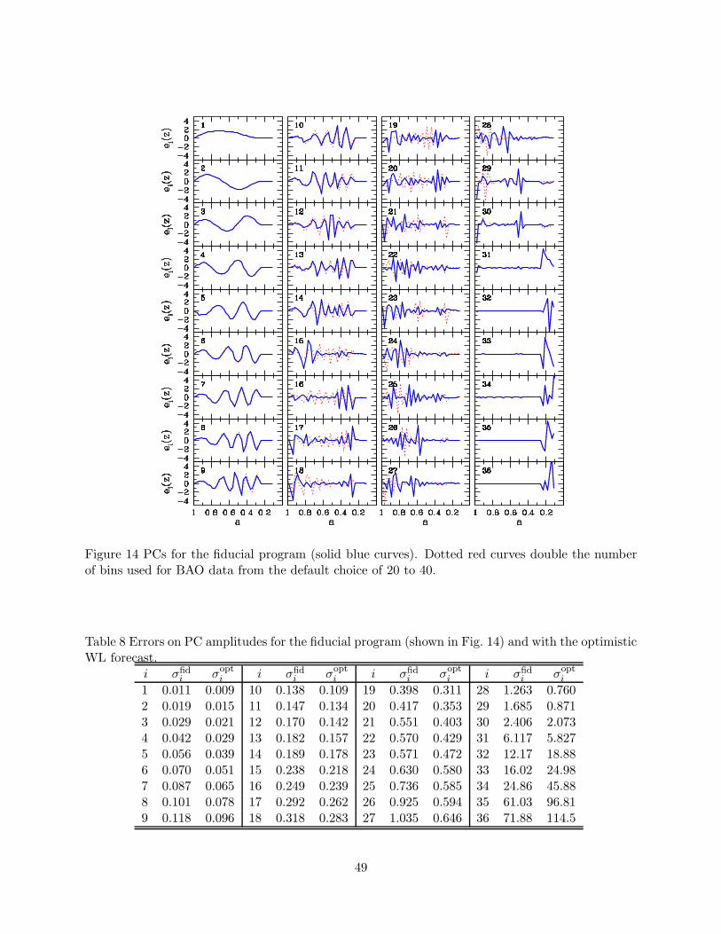
Figure 14 PCs for the fiducial program (solid blue curves). Dotted red curves double the numberof bins used for BAO data from the default choice of 20 to 40.

Table 8 Errors on PC amplitudes for the fiducial program (shown in Fig. 14) and with the optimisticWL forecast.

i σfidi σopt

i i σfidi σopt

i i σfidi σopt

i i σfidi σopt

i

1 0.011 0.009 10 0.138 0.109 19 0.398 0.311 28 1.263 0.7602 0.019 0.015 11 0.147 0.134 20 0.417 0.353 29 1.685 0.8713 0.029 0.021 12 0.170 0.142 21 0.551 0.403 30 2.406 2.0734 0.042 0.029 13 0.182 0.157 22 0.570 0.429 31 6.117 5.8275 0.056 0.039 14 0.189 0.178 23 0.571 0.472 32 12.17 18.886 0.070 0.051 15 0.238 0.218 24 0.630 0.580 33 16.02 24.987 0.087 0.065 16 0.249 0.239 25 0.736 0.585 34 24.86 45.888 0.101 0.078 17 0.292 0.262 26 0.925 0.594 35 61.03 96.819 0.118 0.096 18 0.318 0.283 27 1.035 0.646 36 71.88 114.5

49

few PCs. For the fiducial WL systematics, reducing WL errors helps to better measure several ofthe highest-variance PCs, but it makes little difference to the well measured PCs. Reducing BAOerrors tightens constraints on nearly all of the PCs, with the greatest impact in the intermediaterange between the SN and WL contributions. Assuming the optimistic WL errors gives muchgreater weight to WL improvements, which now produce the largest improvement in the firstfive PCs (right panel of Figure 15). The trends for reducing SN or BAO errors are similar tobefore, but the magnitude of their effect is smaller because they are competing with tighter WLconstraints. The trends for the σ−2

i ratios of the best-measured PCs mirror those shown for theDETF FoM in Figure 5. With the fiducial WL systematics, BAO measurements have the greatestleverage, followed by SN, and the impact of reducing WL errors is small. With the optimistic WLsystematics, on the other hand, reducing WL errors makes the largest difference, followed by BAO,followed by SN.

Figure 15 Ratios of inverse variances of PC amplitudes for variants of the fiducial program to thefiducial inverse variances (points and solid curves). Each variant divides SN, BAO, or WL errorsby a factor of 2 while keeping other probes fixed at the fiducial errors. The left panel assumes thedefault WL forecast and the right panel assumes the optimistic version. Dotted curves in the leftpanel use σi instead of σi, which describes how well the amplitudes of the fiducial set of PCs areexpected to be measured by some variant of the fiducial forecast.

Dotted curves in the left hand panel show the σ−2i ratios when we fix the PCs to be those of the

fiducial program. In this case, the PC errors for the improved programs are no longer uncorrelated,but the correlation coefficient of errors among any pair of PCs is less than 0.5 in nearly all cases.Results are similar to before except for the first component (first two components for BAO). These,of course, show less improvement when they are fixed to be those of the fiducial program ratherthan shifting to be the components best determined by the improved data.

Other figures of merit for PC constraints have been defined in the literature, each of which maybe useful for different purposes. These include the determinant of Fw, which characterizes the totalvolume of parameter space allowed by a particular combination of experiments, in analogy to theDETF FoM for the w0–wa parameter space, and the sum of the inverse variances of the PCs, whichis typically less sensitive to changes in the errors of the most weakly constrained PCs (Huterer

50

Figure 16 Ratios of inverse variances of PC amplitudes of Stage IV to those of Stage III, assumingeither the fiducial or optimistic versions of the Stage IV WL forecast.

and Turner, 2001; Albrecht et al., 2006; Albrecht and Bernstein, 2007; Wang, 2008; Barnard et al.,2008; Albrecht et al., 2009; Crittenden et al., 2009; Amara and Kitching, 2010; Mortonson et al.,2010; Shapiro et al., 2010; Trotta et al., 2010; March et al., 2011).

Examples of these FoMs for the fiducial program and the variants considered in Figure 15 arelisted in Table 9. Here we allow the PC basis to change with the forecast assumptions, so Fw isdiagonal and detFw =

∏36i=1 σ−2

i . As with the ratios of PC variances in Figure 15, we restrict thevariances to be less than unity by replacing σ−2

i → 1 + σ−2i . The other FoM, computed as the sum

of inverse variances, requires no such prior because PCs with large variances contribute negligiblyto the sum. Note that the choice of PC FoM definition can affect decisions about whether oneexperiment or another is optimal; for example, halving WL errors (assuming fiducial systematics)relative to the fiducial model increases the detFw FoM more than halving SN errors, but theopposite is true for the sum of inverse variances, which favors improvements in the best-measuredPCs and more closely tracks the DETF FoM. In this case, at least, we regard the latter measureas a better diagnostic, since the improvements for PCs that are poorly measured in any case seemunlikely to reveal departures from a cosmological constant or other simple dark energy models.

Table 9 Examples of PC FoMs for selected forecasts, with the DETF FoM for comparison.

Forecast case log∏36

i=1

(1 + σ−2

i

)1/2(∑36

i=1 σ−2i )1/2 [σ(wp)σ(wa)]

−1

[SN,BAO,WL,CMB] 21.1 116 533[SN/2,BAO,WL,CMB] 21.6 153 903[SN,BAO/2,WL,CMB] 27.9 181 1070[SN,BAO,WL/2,CMB] 22.2 133 671[SN,BAO,WL-opt,CMB] 23.7 150 687[SN/2,BAO,WL-opt,CMB] 24.1 180 981[SN,BAO/2,WL-opt,CMB] 29.5 201 1129[SN,BAO,WL-opt/2,CMB] 26.5 235 1309

51

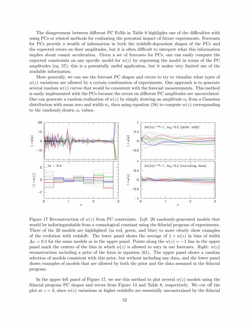
The disagreement between different PC FoMs in Table 9 highlights one of the difficulties withusing PCs or related methods for evaluating the potential impact of future experiments. Forecastsfor PCs provide a wealth of information in both the redshift-dependent shapes of the PCs andthe expected errors on their amplitudes, but it is often difficult to interpret what this informationimplies about cosmic acceleration. Given a set of forecasts for PCs, one can easily compute theexpected constraints on any specific model for w(z) by expressing the model in terms of the PCamplitudes (eq. 57); this is a potentially useful application, but it makes very limited use of theavailable information.

More generally, we can use the forecast PC shapes and errors to try to visualize what types ofw(z) variations are allowed by a certain combination of experiments. One approach is to generateseveral random w(z) curves that would be consistent with the forecast measurements. This methodis easily implemented with the PCs because the errors on different PC amplitudes are uncorrelated.One can generate a random realization of w(z) by simply drawing an amplitude αi from a Gaussiandistribution with mean zero and width σi, then using equation (58) to compute w(z) correspondingto the randomly-drawn αi values.

Figure 17 Reconstruction of w(z) from PC constraints. Left: 20 randomly-generated models thatwould be indistinguishable from a cosmological constant using the fiducial program of experiments.Three of the 20 models are highlighted (in red, green, and blue) to more clearly show examplesof the evolution with redshift. The lower panel shows the average of 1 + w(z) in bins of width∆z = 0.4 for the same models as in the upper panel. Points along the w(z) = −1 line in the upperpanel mark the centers of the bins in which w(z) is allowed to vary in our forecasts. Right: w(z)reconstruction including a prior of the form in equation (61). The upper panel shows a randomselection of models consistent with this prior, but without including any data, and the lower panelshows examples of models that are allowed by both the prior and the data assumed in the fiducialprogram.

In the upper left panel of Figure 17, we use this method to plot several w(z) models using thefiducial program PC shapes and errors from Figure 14 and Table 8, respectively. We cut off theplot at z = 3, since w(z) variations at higher redshifts are essentially unconstrained by the fiducial

52

experiments. Even at lower redshifts, though, the allowed w(z) variations are enormous, with wi

values often changing by 10 or more from one bin to the next. (Recall that our prior correspondsto a Gaussian of width σwi

≈ 63 per bin, eq. 55.) Compared to the ∼ 1.5% constraints on wp inthe w0–wa model, this forecast looks rather depressing. The consequence of allowing the equationof state to be a free function of redshift is that it is nearly impossible to say with any certaintywhat the value of w is at a specific redshift, because rapid oscillations in w(z) have tiny effects onobservables. The allowed range of variations would be even larger if we considered a model withfiner ∆a bins.

The large variations of w(z) in Figure 17 are driven by the poorly constrained PCs, which havemany oscillations in w(z), peak-to-peak amplitudes |∆w| ∼ 4, and normalization uncertaintiesσi ∼ 0.1 − 2.4 (see Figure 14 and Table 8). The lower left panel of Figure 17 shows these w(z)realizations averaged over bins of width ∆z = 0.4, which vastly reduces the range of variations,especially at z ∼ 1. However, the dispersion of w(z) in the bins centered at z = 0.6 and z = 1 isstill about 0.25.

Instead of averaging w(z) over wide redshift bins, one can impose a theoretical prejudice formodels with smoothly-varying equations of state by adding an off-diagonal prior to the Fishermatrix, imposing correlations among the wi that are closely separated in redshift. Here we followCrittenden et al. (2009), but we modify their method to use scale factor rather than redshift as theindependent variable, adopting a correlation function

ξ(|ai − aj |) =(∆w)2

π∆ac

[1 +

(ai − aj

∆ac

)2]−1

, (60)

where ∆w sets the amplitude of allowed w(z) variations and ∆ac is the correlation length. Followingthe calculation in Crittenden et al. (2009), the covariance matrix for the wi bins, which is the inverseof the prior Fisher matrix for those parameters, is

[F priorij ]−1

(i,j≤36) =(∆w)2∆ac

π∆a2

x+ tan−1 x+ + x− tan−1 x− − 2x tan−1 x + ln

1 + x2

√(1 + x2

+)(1 + x2−)

,

(61)where x = |i − j|∆a/∆ac, x+ = (|i − j| + 1)∆a/∆ac, and x− = (|i − j| − 1)∆a/∆ac. In thelimit ∆ac → 0, this reduces to our default diagonal prior on the wi parameters with width σwi

=∆w/

√∆a.

The upper right panel of Figure 17 shows models randomly drawn from this prior with ∆w/√

∆a =1 and ∆ac = 0.2. The influence of the correlation function is clearly evident in the smoother, lower-amplitude variations of w(z) in these models, and yet the range of possible models is still muchgreater than for simpler parameterizations like w0–wa. Combining this prior with the assumeddata set of the fiducial Stage IV program, we obtain the w(z) realizations plotted in the lower rightpanel of Figure 17. Even more so than averaging w(z) in wide redshift bins, including this type ofprior significantly narrows the constraints on w(z).

Our constraints on general w(z) models account for the possibility of modified gravity bymarginalizing over the structure growth parameters ∆γ and ln G9. If we instead restrict our anal-ysis to GR by fixing ∆γ = ln G9 = 0, the main effect is that the dark energy equation of state athigh redshifts, w(3 < z < 9), is better constrained since the CMB measurement of the power spec-trum amplitude at z ∼ 1000 can be more directly related to WL measurements of growth at lowerredshifts. Because of the additional CMB constraint on the distance to the last scattering surface,w(3 < z < 9) is strongly correlated with Ωk, and therefore assuming GR considerably improves the

53

determination of spatial curvature in the binned w(z) parameterization. For our fiducial forecasts,assuming ∆γ = ln G9 = 0 lowers σΩk

by a factor of ∼ 5 (0.0125 → 0.0025); note that this is stillseveral times larger than the error in Ωk for the simpler ΛCDM or w0–wa forecasts.

4. Conclusions

Appendix A. Acronym Glossary

ACT = Atacama Cosmology TelescopeADEPT = Advanced Dark Energy Physics TelescopeBAO = Baryon Acoustic OscillationsBOSS = Baryon Oscillation Spectroscopic SurveyCMB = Cosmic Microwave BackgroundDES = Dark Energy SurveyDESTINY = Dark Energy Space TelescopeDUNE = Dark Universe ExplorerESA = European Space AgencyGR = General RelativityHETDEX = Hobby-Eberly Telescope Dark Energy ExperimentJDEM = Joint Dark Energy MissionJEDI = Joint Efficient Dark-energy InvestigationLASST = Large Area Synoptic Survey TelescopeLSST = Large Synoptic Survey TelescopeNASA = National Aeronautics and Space AdministrationNOAO = National Optical Astronomy ObservatoriesPan-STARRS = Panoramic Survey Telescope and Rapid Response SystemSDSS = Sloan Digital Sky SurveySKA = Square Kilometer ArraySNAP = Supernova Acceleration ProbeSPT = South Pole Telescope

References

, 2006. Planck: The scientific programme.

Abazajian, K. N., et al., 2009. The Seventh Data Release of the Sloan Digital Sky Survey. Astrophys.J. Suppl. 182, 543–558.

Albrecht, A., Bernstein, G., 2007. Evaluating dark energy probes using multidimensional darkenergy parameters. Phys. Rev. D75, 103003.

Albrecht, A., et al., 2006. Report of the Dark Energy Task Force.

Albrecht, A., et al., 2009. Findings of the Joint Dark Energy Mission Figure of Merit ScienceWorking Group.

Amara, A., Kitching, T., 2010. Figures of Merit for Testing Standard Models: Application to DarkEnergy Experiments in Cosmology.

Amendola, L., Quercellini, C., Giallongo, E., 2005. Constraints on perfect fluid and scalar field darkenergy models from future redshift surveys. Mon. Not. Roy. Astron. Soc. 357, 429–439.

54

Bardeen, J. M., Bond, J. R., Kaiser, N., Szalay, A. S., 1986. The Statistics of Peaks of GaussianRandom Fields. Astrophys. J. 304, 15–61.

Barnard, M., Abrahamse, A., Albrecht, A., Bozek, B., Yashar, M., 2008. A measure of the impactof future dark energy experiments based on discriminating power among quintessence models.Phys. Rev. D78, 043528.

Bennett, C. L., et al., 2003. First Year Wilkinson Microwave Anisotropy Probe (WMAP) Observa-tions: Preliminary Maps and Basic Results. Astrophys. J. Suppl. 148, 1.

Berlind, A. A., Weinberg, D. H., 2002. The Halo Occupation Distribution: Towards an EmpiricalDetermination of the Relation Between Galaxies and Mass. Astrophys. J. 575, 587–616.

Blanchard, A., 2010. Evidence for the Fifth Element Astrophysical status of Dark Energy. Astron.Astrophys. Rev. 18, 595–645.

Bond, J. R., Cole, S., Efstathiou, G., Kaiser, N., 1991. Excursion set mass functions for hierarchicalGaussian fluctuations. Astrophys. J. 379, 440.

Bucher, M., Goldhaber, A. S., Turok, N., 1995. An open universe from inflation. Phys. Rev. D52,3314–3337.

Caldwell, R. R., Linder, E. V., 2005. The limits of quintessence. Phys. Rev. Lett. 95, 141301.

Carlson, J., White, M., Padmanabhan, N., 2009. A critical look at cosmological perturbation theorytechniques. Phys. Rev. D80, 043531.

Carroll, S. M., 2003. Why is the universe accelerating? ECONF C0307282, TTH09.

Chaboyer, B., 1998. The Age of the Universe. Phys. Rept. 307, 23–30.

Cole, S., Fisher, K. B., Weinberg, D. H., 1994. Fourier analysis of redshift space distortions andthe determination of Omega. Mon. Not. Roy. Astron. Soc. 267, 785.

Cole, S., Kaiser, N., Apr. 1989. Biased clustering in the cold dark matter cosmogony. MNRAS237,1127–1146.

Cole, S., Weinberg, D. H., Frenk, C. S., Ratra, B., 1997. Large-scale structure in COBE-normalizedcold dark matter cosmogonies. Mon. Not. Roy. Astron. Soc. 289, 37.

Cole, S., et al., 2005. The 2dF Galaxy Redshift Survey: Power-spectrum analysis of the final datasetand cosmological implications. Mon. Not. Roy. Astron. Soc. 362, 505–534.

Conroy, C., Wechsler, R. H., Kravtsov, A. V., 2006. Modeling Luminosity-Dependent Galaxy Clus-tering Through Cosmic Time. Astrophys. J. 647, 201–214.

Crittenden, R. G., Pogosian, L., Zhao, G.-B., 2009. Investigating dark energy experiments withprincipal components. JCAP 0912, 025.

de Bernardis, P., et al., 2000. A Flat Universe from High-Resolution Maps of the Cosmic MicrowaveBackground Radiation. Nature 404, 955–959.

de Putter, R., Linder, E. V., 2008. To Bin or Not To Bin: Decorrelating the Cosmic Equation ofState. Astropart. Phys. 29, 424–441.

55

Dick, J., Knox, L., Chu, M., 2006. Reduction of Cosmological Data for the Detection of Time-varying Dark Energy Density. JCAP 0607, 001.

Dicke, R. H., Peebles, P. J. E., Roll, P. G., Wilkinson, D. T., 1965. Cosmic Black-Body Radiation.Astrophys. J. 142, 414–419.

Dodelson, S., 2003. Modern cosmology.

Dvali, G. R., Gabadadze, G., Porrati, M., 2000. 4D gravity on a brane in 5D Minkowski space.Phys. Lett. B485, 208–214.

Efstathiou, G., Jun. 1995. An anthropic argument for a cosmological constant. MNRAS274, L73–L76.

Efstathiou, G., Sutherland, W. J., Maddox, S. J., 1990. The cosmological constant and cold darkmatter. Nature 348, 705–707.

Einstein, A., 1917. Cosmological Considerations in the General Theory of Relativity. Sitzungsber.Preuss. Akad. Wiss. Berlin (Math. Phys. ) 1917, 142–152.

Eisenstein, D. J., et al., 2005. Detection of the Baryon Acoustic Peak in the Large-Scale CorrelationFunction of SDSS Luminous Red Galaxies. Astrophys. J. 633, 560–574.

Freedman, W. L., et al., 2009. The Carnegie Supernova Project: First Near-Infrared Hubble Dia-gram to z 0.7. Astrophys. J. 704, 1036–1058.

Freese, K., 2005. Cardassian expansion: Dark energy density from modified Friedmann equations.New Astron. Rev. 49, 103–109.

Freese, K., Lewis, M., 2002. Cardassian Expansion: a Model in which the Universe is Flat, MatterDominated, and Accelerating. Phys. Lett. B540, 1–8.

Frieman, J., Turner, M., Huterer, D., 2008a. Dark Energy and the Accelerating Universe. Ann.Rev. Astron. Astrophys. 46, 385–432.

Frieman, J. A., 1996. Weak Lensing and the Measurement of q0 from Type Ia Supernovae.

Frieman, J. A., et al., 2008b. The Sloan Digital Sky Survey-II Supernova Survey: Technical Sum-mary. Astron. J. 135, 338–347.

Gehrels, N., 2010. The Joint Dark Energy Mission (JDEM) Omega.

Griest, K., 2002. Toward a possible solution to the cosmic coincidence problem. Phys. Rev. D66,123501.

Gunn, J. E., Gott, III, J. R., 1972. On the infall of matter into cluster of galaxies and some effectson their evolution. Astrophys. J. 176, 1–19.

Guth, A. H., 1981. The Inflationary Universe: A Possible Solution to the Horizon and FlatnessProblems. Phys. Rev. D23, 347–356.

Hamilton, A. J. S., 1997. Linear Redshift Distortions: A Review.

Hamuy, M., et al., 2006. The Carnegie Supernova Project: The Low-Redshift Survey. Publ. Astron.Soc. Pac. 118, 2–20.

56

Hanany, S., et al., 2000. MAXIMA-1: A Measurement of the Cosmic Microwave BackgroundAnisotropy on angular scales of 10 arcminutes to 5 degrees. Astrophys. J. 545, L5.

Heitmann, K., White, M., Wagner, C., Habib, S., Higdon, D., 2010. The Coyote Universe I: Preci-sion Determination of the Nonlinear Matter Power Spectrum. Astrophys. J. 715, 104–121.

Hogg, D. W., 1999. Distance measures in cosmology.

Hu, W., 2002. Dark Energy and Matter Evolution from Lensing Tomography. Phys. Rev. D66,083515.

Hu, W., 2005. Dark Energy Probes in Light of the CMB. ASP Conf. Ser. 339, 215.

Hu, W., Jain, B., 2004. Joint Galaxy-Lensing Observables and the Dark Energy. Phys. Rev. D70,043009.

Hubble, E., 1929. A relation between distance and radial velocity among extra–galactic nebulae.Proc. Nat. Acad. Sci. 15, 168–173.

Huterer, D., Cooray, A., 2005. Uncorrelated Estimates of Dark Energy Evolution. Phys. Rev. D71,023506.

Huterer, D., Starkman, G., 2003. Parameterization of dark-energy properties: A principal- compo-nent approach. Phys. Rev. Lett. 90, 031301.

Huterer, D., Turner, M. S., 2001. Probing the dark energy: Methods and strategies. Phys. Rev.D64, 123527.

Jain, B., Khoury, J., 2010. Cosmological Tests of Gravity. Annals Phys. 325, 1479–1516.

Jimenez, R., Loeb, A., 2002. Constraining Cosmological Parameters Based on Relative GalaxyAges. Astrophys. J. 573, 37–42.

Kaiser, N., 1984. On the Spatial correlations of Abell clusters. Astrophys. J. 284, L9–L12.

Kaiser, N., 1987. Clustering in real space and in redshift space. Mon. Not. Roy. Astron. Soc. 227,1–27.

Kessler, R., et al., 2009. First-year Sloan Digital Sky Survey-II (SDSS-II) Supernova Results: Hub-ble Diagram and Cosmological Parameters. Astrophys. J. Suppl. 185, 32–84.

Kitching, T. D., Amara, A., 2009. Fisher Matrix Decomposition for Dark Energy Prediction.

Komatsu, E., et al., 2009. Five-Year Wilkinson Microwave Anisotropy Probe (WMAP) Observa-tions:Cosmological Interpretation. Astrophys. J. Suppl. 180, 330–376.

Komatsu, E., et al., 2011. Seven-Year Wilkinson Microwave Anisotropy Probe (WMAP) Observa-tions: Cosmological Interpretation. Astrophys. J. Suppl. 192, 18.

Krauss, L. M., Turner, M. S., 1995. The cosmological constant is back. Gen. Rel. Grav. 27, 1137–1144.

Kravtsov, A. V., et al., 2004. The Dark Side of the Halo Occupation Distribution. Astrophys. J.609, 35–49.

57

Larson, D., et al., 2011. Seven-Year Wilkinson Microwave Anisotropy Probe (WMAP) Observations:Power Spectra and WMAP-Derived Parameters. Astrophys. J. Suppl. 192, 16.

Lewis, A., Challinor, A., Lasenby, A., 2000. Efficient Computation of CMB anisotropies in closedFRW models. Astrophys. J. 538, 473–476.

Lightman, A. P., Schechter, P. L., Dec. 1990. The Omega dependence of peculiar velocities inducedby spherical density perturbations. ApJS74, 831–+.

Linde, A. D., 1987. Eternally existing self-reproducing inflationary universe. Physica Scripta VolumeT 15, 169–175.

Linder, E. V., 2003a. Exploring the expansion history of the universe. Phys. Rev. Lett. 90, 091301.

Linder, E. V., 2003b. Mapping the Dark Energy Equation of State.

Linder, E. V., 2005. Cosmic growth history and expansion history. Phys. Rev. D72, 043529.

Linder, E. V., 2007. Theory Challenges of the Accelerating Universe. J. Phys. A40, 6697.

Linder, E. V., 2010. Frontiers of Dark Energy.

Maddox, S. J., Efstathiou, G., Sutherland, W. J., Loveday, J., 1990. Galaxy correlations on largescales. Mon. Not. Roy. Astron. Soc. 242, 43–49.

Mantz, A., Allen, S. W., Rapetti, D., Ebeling, H., 2010. The Observed Growth of Massive GalaxyClusters I: Statistical Methods and Cosmological Constraints. Mon. Not. Roy. Astron. Soc. 406,1759–1772.

March, M. C., Trotta, R., Amendola, L., Huterer, D., 2011. Robustness to systematics for futuredark energy probes.

Martel, H., Shapiro, P. R., Weinberg, S., 1998. Likely Values of the Cosmological Constant. Astro-phys. J. 492, 29.

Maturi, M., Mignone, C., 2009. An optimal basis system for cosmology: data analysis and newparameterisation. Astron. Astrophys. 508, 45M.

Mo, H. J., White, S. D. M., 1996. An Analytic model for the spatial clustering of dark matter halos.Mon. Not. Roy. Astron. Soc. 282, 347.

Mortonson, M., Hu, W., Huterer, D., 2009a. Hiding dark energy transitions at low redshift. Phys.Rev. D80, 067301.

Mortonson, M. J., Hu, W., Huterer, D., 2009b. Falsifying Paradigms for Cosmic Acceleration. Phys.Rev. D79, 023004.

Mortonson, M. J., Huterer, D., Hu, W., 2010. Figures of merit for present and future dark energyprobes. Phys. Rev. D82, 063004.

Mould, J. R., et al., 2000. The HST Key Project on the Extragalactic Distance Scale. XXVIII.Combining the Constraints on the Hubble Constant. Astrophys. J. 529, 786–794.

58

Netterfield, C. B., Devlin, M. J., Jarosik, N., Page, L., Wollack, E. J., 1997. A Measurement of theAngular Power Spectrum of the Anisotropy in the Cosmic Microwave Background. Astrophys.J. 474, 47.

Norberg, P., et al., 2001. The 2dF Galaxy Redshift Survey: Luminosity dependence of galaxyclustering s. Mon. Not. Roy. Astron. Soc. 328, 64.

Ostriker, J. P., Steinhardt, P. J., 1995. The Observational case for a low density universe with anonzero cosmological constant. Nature 377, 600–602.

Peebles, P. J. E., 1980. The large-scale structure of the universe.

Peebles, P. J. E., Ratra, B., 2003. The cosmological constant and dark energy. Rev. Mod. Phys.75, 559–606.

Penzias, A. A., Wilson, R. W., 1965. A Measurement of excess antenna temperature at 4080- Mc/s.Astrophys. J. 142, 419–421.

Perlmutter, S., et al., 1997. Measurements of the Cosmological Parameters Omega and Lambdafrom the First 7 Supernovae at z ¿= 0.35. Astrophys. J. 483, 565.

Perlmutter, S., et al., 1999. Measurements of Omega and Lambda from 42 High-Redshift Super-novae. Astrophys. J. 517, 565–586.

Phillips, M. M., 1993. The absolute magnitudes of Type IA supernovae. Astrophys. J. 413, L105–L108.

Press, W. H., Schechter, P., 1974. Formation of galaxies and clusters of galaxies by selfsimilargravitational condensation. Astrophys. J. 187, 425–438.

Ratra, B., Peebles, P. J. E., 1988. Cosmological Consequences of a Rolling Homogeneous ScalarField. Phys. Rev. D37, 3406.

Reid, B. A., et al., 2010a. Baryon Acoustic Oscillations in the Sloan Digital Sky Survey DataRelease 7 Galaxy Sample. Mon. Not. Roy. Astron. Soc. 401, 2148–2168.

Reid, B. A., et al., 2010b. Cosmological Constraints from the Clustering of the Sloan Digital SkySurvey DR7 Luminous Red Galaxies. Mon. Not. Roy. Astron. Soc. 404, 60–85.

Riess, A. G., Livio, M., 2006. The First Type Ia Supernovae: An Empirical Approach to TamingEvolutionary Effects In Dark Energy Surveys from SNe Ia at z¿2. Astrophys. J. 648, 884–889.

Riess, A. G., Press, W. H., Kirshner, R. P., 1996. A Precise distance indicator: Type Ia supernovamulticolor light curve shapes. Astrophys. J. 473, 88.

Riess, A. G., et al., 1998. Observational Evidence from Supernovae for an Accelerating Universeand a Cosmological Constant. Astron. J. 116, 1009–1038.

Riess, A. G., et al., 2007. New Hubble Space Telescope Discoveries of Type Ia Supernovae at z > 1:Narrowing Constraints on the Early Behavior of Dark Energy. Astrophys. J. 659, 98–121.

Riess, A. G., et al., 2009. A Redetermination of the Hubble Constant with the Hubble SpaceTelescope from a Differential Distance Ladder. Astrophys. J. 699, 539–563.

59

Rozo, E., et al., 2010. Cosmological Constraints from the SDSS maxBCG Cluster Catalog. Astro-phys. J. 708, 645–660.

Schechter, P., 1976. An analytic expression for the luminosity function for galaxies. Astrophys. J.203, 297–306.

Schmidt, B. P., et al., 1998. The High-Z Supernova Search: Measuring Cosmic Deceleration andGlobal Cur vature of the Universe Using Type Ia Supernovae. Astrophys. J. 507, 46–63.

Scoccimarro, R., 2004. Redshift-Space Distortions, Pairwise Velocities and Nonlinearities. Phys.Rev. D70, 083007.

Scoccimarro, R., Sheth, R. K., Hui, L., Jain, B., 2001. How Many Galaxies Fit in a Halo? Con-straints on Galaxy Formation Efficiency from Spatial Clustering. Astrophys. J. 546, 20–34.

Seljak, U., 2000. Analytic model for galaxy and dark matter clustering. Mon. Not. Roy. Astron.Soc. 318, 203.

Seo, H.-J., Eisenstein, D. J., 2007. Improved forecasts for the baryon acoustic oscillations andcosmological distance scale. Astrophys. J. 665, 14–24.

Shapiro, C., Dodelson, S., Hoyle, B., Samushia, L., Flaugher, B., 2010. Will Multiple Probes ofDark Energy find Modified Gravity? Phys. Rev. D82, 043520.

Sheth, R. K., Tormen, G., 1999. Large scale bias and the peak background split. Mon. Not. Roy.Astron. Soc. 308, 119.

Simpson, F., Bridle, S., 2006. The redshift sensitivities of dark energy surveys. Phys. Rev. D73,083001.

Skordis, C., Albrecht, A., 2002. Planck-scale quintessence and the physics of structure formation.Phys. Rev. D66, 043523.

Song, Y.-S., Hu, W., Sawicki, I., 2007. The large scale structure of f(R) gravity. Phys. Rev. D75,044004.

Steinhardt, P. J., Wang, L.-M., Zlatev, I., 1999. Cosmological tracking solutions. Phys. Rev. D59,123504.

Stubbs, C. W., Tonry, J. L., 2006. Toward 1Calibration of Astronomical Telescopes and Detectors.Astrophys. J. 646, 1436–1444.

Sunyaev, R. A., Zeldovich, Y. B., Apr. 1970. Small-Scale Fluctuations of Relic Radiation. Ap &SS7, 3–19.

Susskind, L., 2003. The anthropic landscape of string theory.

Tang, J., Abdalla, F. B., Weller, J., 2008. Complementarity of Future Dark Energy Probes.

Tegmark, M., Rees, M. J., 1998. Why is the CMB fluctuation level 10−5? Astrophys. J. 499,526–532.

Tegmark, M., et al., 2004. The 3D power spectrum of galaxies from the SDSS. Astrophys. J. 606,702–740.

60

Tinker, J. L., et al., 2008. Toward a halo mass function for precision cosmology: the limits ofuniversality. Astrophys. J. 688, 709–728.

Tinker, J. L., et al., 2010. The Large Scale Bias of Dark Matter Halos: Numerical Calibration andModel Tests. Astrophys. J. 724, 878–886.

Trotta, R., Kunz, M., Liddle, A. R., 2010. Designing Decisive Detections.

Vikhlinin, A., et al., 2009. Chandra Cluster Cosmology Project III: Cosmological Parameter Con-straints. Astrophys. J. 692, 1060–1074.

Wang, L.-M., Steinhardt, P. J., 1998. Cluster Abundance Constraints on Quintessence Models.Astrophys. J. 508, 483–490.

Wang, Y., 1999. Analytical Modeling of the Weak Lensing of Standard Candles. Astrophys. J. 525,651.

Wang, Y., 2008. Figure of Merit for Dark Energy Constraints from Current Observational Data.Phys. Rev. D77, 123525.

Wang, Y., Tegmark, M., 2005. Uncorrelated Measurements of the Cosmic Expansion History andDark Energy from Supernovae. Phys. Rev. D71, 103513.

Weinberg, D. H., 2005. Dark Energy: The Observational Challenge. New Astron. Rev. 49, 337–345.

Weinberg, S., 1989. The cosmological constant problem. Rev. Mod. Phys. 61, 1–23.

Yoo, J., Weinberg, D. H., Tinker, J. L., Zheng, Z., Warren, M. S., 2009. Extending Recovery of thePrimordial Matter Power Spectrum. Astrophys. J. 698, 967–985.

Zehavi, I., et al., 2005. The Luminosity and Color Dependence of the Galaxy Correlation Function.Astrophys. J. 630, 1–27.

Zehavi, I., et al., 2010. Galaxy Clustering in the Completed SDSS Redshift Survey: The Dependenceon Color and Luminosity.

61