Prepared for submission to JCAP

Observational constraints onK-inflation models

Sheng Li and Andrew R. Liddle

Astronomy Centre, University of Sussex, Brighton BN1 9QH, United Kingdom

E-mail: sl277@sussex.ac.uk, a.liddle@sussex.ac.uk

Abstract. We extend the ModeCode software of Mortonson, Peiris and Easther [1] toenable numerical computation of perturbations in K-inflation models, where the scalarfield no longer has a canonical kinetic term. Focussing on models where the kineticand potential terms can be separated into a sum, we compute slow-roll predictions forvarious models and use these to verify the numerical code. A Markov chain MonteCarlo analysis is then used to impose constraints from WMAP7 data on the additionof a term quadratic in the kinetic energy to the Lagrangian of simple chaotic inflationmodels. For a quadratic potential, the data do not discriminate against addition of sucha term, while for a quartic (λφ4) potential inclusion of such a term is actually favoured.Overall, constraints on such a term from present data are found to be extremely weak.

Keywords: inflation

arX

iv:1

204.

6214

v3 [

astr

o-ph

.CO

] 2

4 Ju

l 201

2

Contents

1 Introduction 1

2 The K-inflation model 22.1 Background field equations and sound speed 22.2 Perturbation mode equations 32.3 Power spectra and observables 4

3 Slow-roll predictions 53.1 General prediction without specifying a potential 53.2 Predictions for specific models through e-folding N 6

4 ModeCode for K-inflation 94.1 Brief description of ModeCode 104.2 Modifications needed for K-inflation 104.3 Comparison tests 11

4.3.1 Recovery of ModeCode results for K(X) = X 114.3.2 Recovery of slow-roll results 11

5 Parameter explorations with MCMC methodology 125.1 Global settings and initial conditions 125.2 Choice of models 125.3 Overview of effects from additional kinetic terms 135.4 Interpretation of MCMC explorations 13

6 Conclusions 15

1 Introduction

Observations, especially including those from the Wilkinson Microwave AnisotropyProbe (WMAP) [2–5], are beginning to impose useful constraints on inflationary cos-mologies. In particular, a number of papers have made detailed evaluations of con-straints on the simplest inflation models, featuring a single canonically-normalizedscalar field with unknown potential V (φ), see for example Refs. [4, 6–17].

Staying with the single-field paradigm, a more general scenario is available throughthe K-inflation paradigm. This retains minimal coupling of the scalar field to gravity,but allows the action to have an arbitrary dependence on the field’s kinetic energy aswell as on its value. This introduces new features, including a sound speed less thanthe speed of light which may enhance the non-gaussianity in the models. Our aimin this paper is to impose observational constraints on versions of this more generalsingle-field scenario.

– 1 –

Our strategy is to modify the ModeCode program of Mortonson et al. [1], whichsolves the inflationary perturbation mode equations numerically and then interfaces tothe CAMB [18] and CosmoMC [19] packages in order to compute the correspondingmicrowave anisotropies and compare to observational data. This entails a number ofmodifications to the way that ModeCode handles both the background (homogeneous)evolution equations and the perturbation equations. In this paper we will focus onthe simplest case where the kinetic and potential terms remain sum-separable, andconsider only simple forms for each. For the potential we will consider the simplestchaotic inflation models [20, 21], based on quadratic and quartic potentials. For thekinetic term, we will consider simple monomial and polynomial forms, in particularinvestigating constraints on addition of a term quadratic in the kinetic energy to thenormal canonical form. Future work will explore more complicated forms. Modificationof ModeCode to consider specifically the action corresponding to DBI inflation (seeRefs. [22, 23]) has already been carried out in Ref. [24]. Comparison of K-inflationmodels to five-year WMAP data using slow-roll methods has been made in Ref. [25].

2 The K-inflation model

The K-inflation model [26, 27] features a single scalar field with the action

S =

∫ √−g p(φ,X)d4x , (2.1)

where φ is the field value and X ≡ (1/2)∂µφ∂µφ. The function p will play the role

of the pressure. A canonical scalar field has p(φ,X) = X − V (φ) where V (φ) is thepotential. In this paper we will focus on models where the kinetic and potential termscan be written as a sum:

p(φ,X) = K(X)− V (φ) , (2.2)

where K(X) and V (φ) are both arbitrary functions to be determined from data.Given the Lagrangian p(X,φ) of the considered model, we can obtain observable

consequences by the following approach, closely following Garriga and Mukhanov [27].

2.1 Background field equations and sound speed

We assume the usual Einstein equations and a spatially-flat Robertson–Walker metricwith scale factor a and Hubble parameter H = a/a. We use the reduced Planckmass, defined by M2

Pl = (8πG)−1, to denote the strength of gravity throughout (withc = ~ = 1 as usual).

First, without needing to consider gravity, we can obtain a relationship betweenthe density ρ of the universe and its pressure p,

ρ = −3H(ρ+ p) , (2.3)

which is known as the continuity equation, in which the energy–momentum tensor ischaracterised by the pressure p(X,φ) and the density

ρ(X,φ) = 2Xdp

dX− p (2.4)

– 2 –

of this universe.Second, now invoking a theory of gravity in the form of general relativity, we have

the Friedmann equation for flat cosmologies

H2 =ρ

3M2Pl

. (2.5)

Taking Eq. (2.3) together with Eq. (2.5), we can therefore study the evolution of thescale factor a and the field variable φ.

One important quantity, called the ‘sound speed’, describes the properties of theφ field. Regarding the field as a fluid system, we can introduce c2s as

c2s =p,X

ρ,X

=p,X

2Xp,XX

+ p,X

, (2.6)

where the comma denotes the partial derivative with respect to X.

2.2 Perturbation mode equations

The background state for the field φ is given by Eqs. (2.3) and (2.5). However, con-frontation of inflationary models with data requires us to evaluate the perturbationsthey predict. We will just quote the two significant equations, first derived by Garrigaand Mukhanov [27]. The scalar and tensor perturbations are described by quantitiesv and u whose Fourier components in the longitudinal gauge satisfy

d2vkdτ 2

+

(c2sk

2 − d2z/dτ 2

z

)vk = 0 (2.7)

d2ukdτ 2

+

(k2 − d2a/dτ 2

a

)uk = 0 (2.8)

respectively. Here, τ is the conformal time, subscript k denotes the momentum space,and the variable k relates to the comoving scale by λ = 2π/k. The curvature pertur-bation ζ is related to v by ζ = v/z, while in a flat universe the background variable zcan be expressed as

z2 =a2(ρ+ p)

c2sH2

. (2.9)

In momentum space, the canonical quantisation modes vk and uk give two differ-ent classes of perturbations, the scalar perturbations measured by vk and the tensor(gravitational wave) perturbations by uk. From Eq. (2.7), we see that cs/H plays therole of the ‘sound horizon’, which the k mode leaves by satisfying csk = aH. Thepower spectrum of the scalar mode can be expressed by

Ps(k) =k3

2π2

∣∣∣vkz

∣∣∣2 , (2.10)

while in Eq. (2.8) the tensor mode leaves the usual horizon by satisfying k = aH, withspectrum

Pt(k) =k3

2π2

∣∣∣uka

∣∣∣2 . (2.11)

– 3 –

2.3 Power spectra and observables

Solving Eq. (2.7) in the slow-roll approximation gives the expression [27]:

Ps =1

8π2M2Pl

H2

εcs

∣∣∣∣csk=aH

, (2.12)

The tensor mode Eq. (2.8) has its usual power spectrum

Pt =2

π2M2Pl

H2

∣∣∣∣k=aH

. (2.13)

Having given the mode equations and their spectra, we can study the two mostinteresting variables, the spectral index ns and the tensor–scalar ratio r. These twoquantities can be constrained by observations, such as the existing WMAP data or theforthcoming Planck satellite results. Their definitions are

ns − 1 ≡ d lnPs

d ln k' −2ε− η − s (2.14)

nt ≡d lnPt

d ln k' −2ε (2.15)

r ≡ Pt

Ps

= 16εcs , (2.16)

where the parameters ε , η , δ , s are all small and defined as

ε = −d lnH

dN; η =

d ln ε

dN; δ = −d ln φ

dN; s =

d ln csdN

, (2.17)

through dN = Hdt, and we additionally give the tensor spectral index nt. Higher-orderversions of these expressions, which we do not use here, have been obtained using theuniform approximation [28].

All these parameters are calculated at the time when mode k leaves its individualhorizon. For the scalar mode k takes the value of aH/cs, while for tensor mode k takesaH. As a result, the relation of d/dN to d/d ln k for the scalars is

d ln k

dN= 1− ε− s . (2.18)

Therefore Eq. (2.14) and Eq. (2.15) are then actually divided by Eq. (2.18), whereass must be taken as zero when adjusting Eq. (2.15) as the sound speed does not enterits horizon-crossing expression.

Note that η in Eq. (2.17) is implicitly a function of the usual slow-roll parametersε = (M2

Pl/2)(V ′/V )2 and η = M2PlV

′′/V and other smaller parameters, such as δ.1 Hereand throughout primes are derivatives with respect to φ. We will discuss its particularexpression in later sections when investigating specific models.

1The full expression is

η = 2ε− 2

(1 +

Xp,XX

p,X

)δ +

p,Xφ

p,X

φ,N

given pressure p = p(X,φ), where , N indicates the derivative with respect to N . In our currentconsideration, the pressure has separable X and φ, so the last term vanishes. The factor of δ in thesecond term can be treated as −(1 + θ), where θ = 1/c2s . Therefore η = 2ε− (1 + θ)δ.

– 4 –

3 Slow-roll predictions

In this section, we use the slow-roll approximation to compute the spectral index ns

and tensor-to-scalar ratio r for various models. These results are of interest in theirown right as they give an indication of the properties of models that will be able to fitthe data. Additionally, we will be able to use them to verify that our modifications toModeCode have been implemented successfully.

3.1 General prediction without specifying a potential

We study models where the Lagrangian takes the form

p(φ,X) = Kn+1Xn − V (φ) , (3.1)

where Kn+1 are constants and n takes integer values.2 Under this kind of action, wecan derive the field equation for the scalar field φ from Eq. (2.3) as

Xρ,X

+ φρ,φ

= −6nKn+1HXn , (3.2)

where the subscript , φ is the derivative with respect to the field.We now discuss what the models predict under the slow-roll scheme. Therefore

by the usual consideration, we assume the density of the universe is dominated by thescalar potential, H2 ∝ ρ ' V and replace all appearances of the Hubble parameterH2 by V . In the field equation Eq. (3.2), we take the first (acceleration) term on theleft-hand side to be much less than the second term. Hence it simplifies to

V ′φ ' −6nKn+1HXn . (3.3)

Within the slow-roll assumption, we can obtain descriptions of the observable quantitiesby means of some parameters. From Eq. (2.17) we can identify ε as ε

Vunder the slow-

roll assumption, where

εV

= −1

2

V ′

V

φ

H. (3.4)

With φ � φ under the slow-roll assumption, for later discussion we give the secondparameter η

Vwhich relates to the first and second-order derivatives of the potential,

ηV

= −V′′

V ′φ

H. (3.5)

By the approximation above, we can find a simple relation between these parameters,

ηV

εV

= 2V V ′′

V ′2, (3.6)

and also we can find the relation

η = 3εV− δ − η

V. (3.7)

2With only a single kinetic term, the coefficient Kn+1 could be removed by rescaling φ, adjustingthe potential, but for later comparison with cases with more than one term we keep it explicit.

– 5 –

From Eq. (3.3), for later evaluation we can write the ratio φ/H as

φ

H= −α(n)

(V ′

V n

)1/(2n−1)

(3.8)

where

α(n) =

(6n−1

nKn+1

M2nPl

)1/(2n−1)

. (3.9)

Then

εV

=1

2α(n)

(V ′2n

V 3n−1

)1/(2n−1)

; ηV

= α(n)

(V ′′(2n−1)

V nV ′2n−2

)1/(2n−1)

. (3.10)

Now we would like to apply the slow-roll approximation to evaluate the mostimportant physical observables. The first is the scalar power spectrum Ps,

Ps ∝2

α(n)cs

(V 5n−2

V ′2n

)1/(2n−1)

, (3.11)

In this case, we can write the spectral index via Eq. (3.11) as

ns − 1 =1

2n− 1[2nη

V− 2(5n− 2)ε

V] . (3.12)

To verify that Eqs. (3.11) and (3.12) are correct for standard inflation, we just need toset n = 1, and then we have the power spectrum

Ps =1

12π2M2Pl

K2V

2εV

, (3.13)

and its corresponding spectral index is ns−1 = 2ηV−6ε

V. As a prediction of Eq. (3.12),

for the simplest non-canonical inflation, in which the kinetic term has the form X2, wecan obtain the power spectrum

Ps =1

12π2M4Pl

(K3V

8

3M4PlV

′4

)1/3

, (3.14)

and its spectral index ns − 1 = (4ηV− 16ε

V)/3.

3.2 Predictions for specific models through e-folding N

Thus far we have obtained the formulae for the scalar power spectrum and its spectralindex without specifying a particular potential type. In this subsection, we continuethe discussion within a class of potential V (φ) = Aφm in the Lagrangian Eq. (3.1),where A denotes the normalisation parameter, and m takes integer values.3

3Following footnote 2, for this form of potential a rescaling of φ to eliminate Kn+1 in the single-termkinetic case would simply renormalize A, which anyway is to be fixed by the density perturbation am-plitude. Hence there is a perfect degeneracy between Kn+1 and A and data can only fix a combinationof them.

– 6 –

The e-folding number N , which measures how much inflation took place, is

N = −∫H dt . (3.15)

After observable scales cross the horizon we have N ∼ 50 until inflation ends. Firstwe evaluate the time variation H dt by the time-shift carried by the scalar field φ andfinally transferred from the gradient change in the potential V (φ)

H dt =H

φdφ =

H

φ

1

V ′dV . (3.16)

So from the definition of N , and taking the above relation along with Eq. (3.8), wecan derive the corresponding relation for N in terms of the scalar potential V (φ) andits derivatives, rather than with φ itself,

N =

∫ e

i

H

φ

1

V ′dV . (3.17)

Under the assumption of slow-roll, by means of the slow-varying parameters, sayEqs. (3.4) and (3.5), we can write Eq. (3.17) as

N = −1

2

∫ e

i

1

ε

dV

V. (3.18)

Here ε (neglecting the subscript) is a function of the potential and its derivativesas well, which have already been denoted by Eqs. (3.4) and (3.5) in the slow-rollapproximation. Connecting N with these two slowly-varying parameters leads to theexpression for spectral index ns.

By taking potential V (φ) = Aφm, we obtain

N =m

β(n,m)

1

γ(n,m)V β(n,m)/m (3.19)

where

β(n,m) =m(n− 1) + 2n

2n− 1; γ(n,m) = α(n)

(mA1/m

)2n/(2n−1). (3.20)

Then, connecting Eqs. (3.4), (3.5) and Eq. (3.19), we can get the relation between theslow-roll parameters and N

εV

=m

2β

1

N; η

V=m− 1

β

1

N. (3.21)

The final formula for the spectral index in Eq. (3.12) is therefore

ns − 1 = −I(n,m)1

N, (3.22)

– 7 –

n = 1 n = 2m = 2 m = 4 m = 2 m = 4

α(n) M2Pl/K2 M2

Pl/K2 (3M4Pl/K3)

1/3 (3M4Pl/K3)

1/3

β(n,m) 2 2 2 8/3

γ(n,m) 4α(1)A 16α(1)A1/2 24/3α(2)A2/3 28/3α(2)A1/3

I(n,m) 2 3 2 5/2

Ps γ(1,2)N2 γ2(1,4)(N/2)3

√3γ(2,2)N

2√

3γ3/2(2,4)(2N/3)5/2

ns

∣∣N=50

0.96 0.94 0.96 0.95

r∣∣N=50

0.16 0.32 0.092 0.14

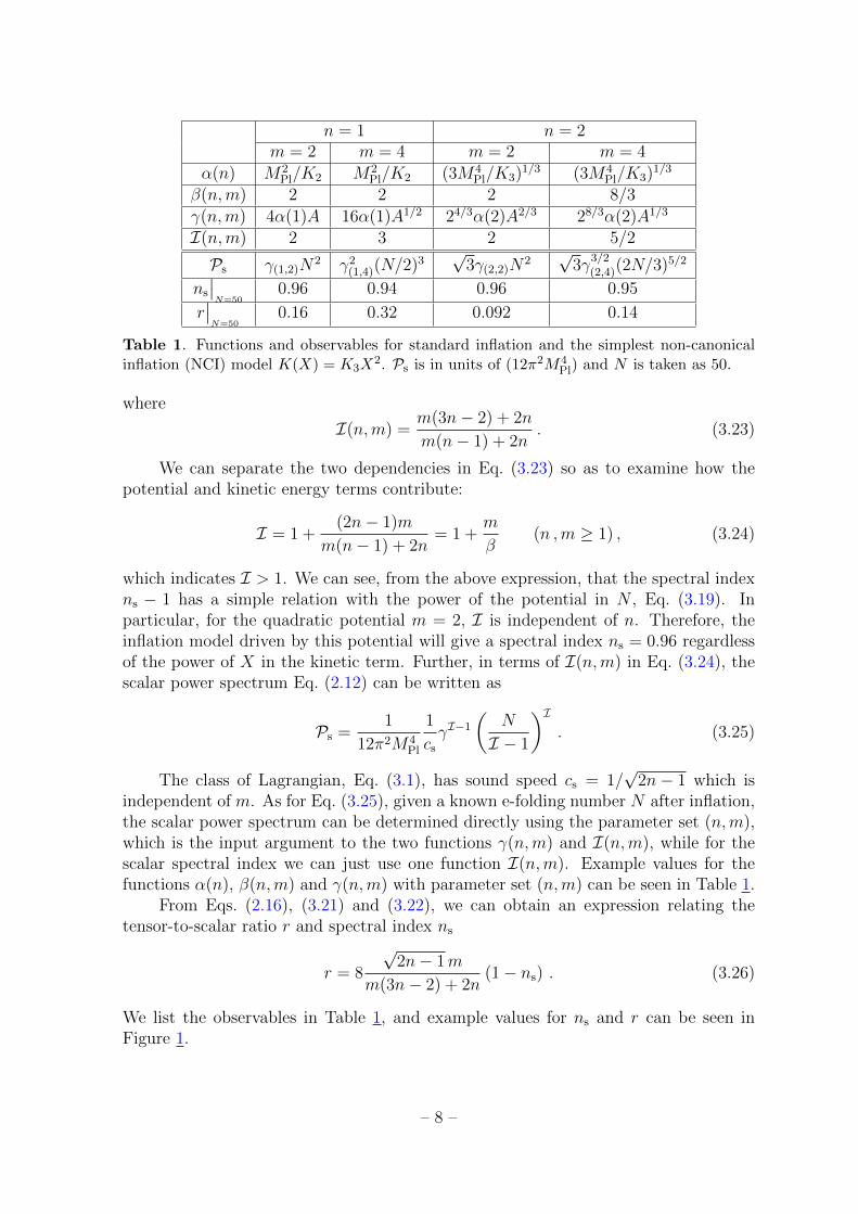
Table 1. Functions and observables for standard inflation and the simplest non-canonicalinflation (NCI) model K(X) = K3X

2. Ps is in units of (12π2M4Pl) and N is taken as 50.

where

I(n,m) =m(3n− 2) + 2n

m(n− 1) + 2n. (3.23)

We can separate the two dependencies in Eq. (3.23) so as to examine how thepotential and kinetic energy terms contribute:

I = 1 +(2n− 1)m

m(n− 1) + 2n= 1 +

m

β(n ,m ≥ 1) , (3.24)

which indicates I > 1. We can see, from the above expression, that the spectral indexns − 1 has a simple relation with the power of the potential in N , Eq. (3.19). Inparticular, for the quadratic potential m = 2, I is independent of n. Therefore, theinflation model driven by this potential will give a spectral index ns = 0.96 regardlessof the power of X in the kinetic term. Further, in terms of I(n,m) in Eq. (3.24), thescalar power spectrum Eq. (2.12) can be written as

Ps =1

12π2M4Pl

1

csγI−1

(N

I − 1

)I. (3.25)

The class of Lagrangian, Eq. (3.1), has sound speed cs = 1/√

2n− 1 which isindependent of m. As for Eq. (3.25), given a known e-folding number N after inflation,the scalar power spectrum can be determined directly using the parameter set (n,m),which is the input argument to the two functions γ(n,m) and I(n,m), while for thescalar spectral index we can just use one function I(n,m). Example values for thefunctions α(n), β(n,m) and γ(n,m) with parameter set (n,m) can be seen in Table 1.

From Eqs. (2.16), (3.21) and (3.22), we can obtain an expression relating thetensor-to-scalar ratio r and spectral index ns

r = 8

√2n− 1m

m(3n− 2) + 2n(1− ns) . (3.26)

We list the observables in Table 1, and example values for ns and r can be seen inFigure 1.

– 8 –

0

0.04

0.08

0.12

0.16

0.2

0.24

0.28

0.32

0.36

0.9 0.91 0.92 0.93 0.94 0.95 0.96 0.97 0.98 0.99 1

r (

Ten

sor

to S

cala

r)

ns (Spectral Index)

Xn - Aφm (1,2)(1,4)(2,2)(2,4)

Figure 1. Slow-roll predictions for the tensor-to-scalar ratio r and the scalar spectral indexns in standard inflation and the simplest NCI model where n = 2 in Eq. (3.1).

For canonical inflation, the known relation ns− 1 = −(m+ 2)/2N is recovered bysetting n = 1. For n = 2, we find

ns − 1 = −4(m+ 1)

m+ 4

1

N. (3.27)

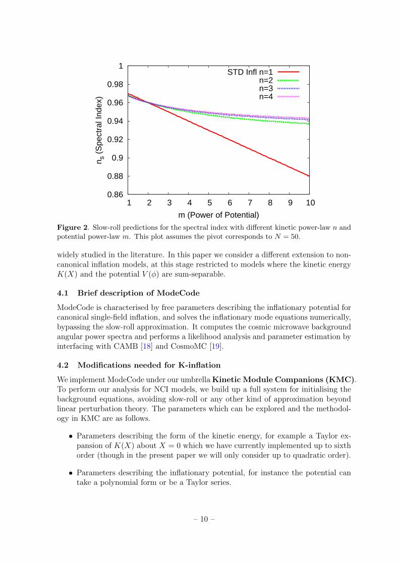
Figure 2 shows the spectral index as a function of m for several n values; when n > 1the spectral index asymptotes to 1− 4/N in the limit of large potential power-law m,unlike the canonical case where 1− ns grows linearly with m and can be large.

4 ModeCode for K-inflation

For single-field canonically-normalized inflation models there are many numerical toolswhich can calculate the primordial power spectra, as well as other characteristics suchas the bispectrum and trispectrum of non-gaussianities. Also many of these tools havebeen interfaced with MCMC codes such as CosmoMC so as to explore the likelihoodand carry out parameter estimation. ModeCode [1] is an example of such a programme,which had also recently been interfaced to the MultiNest model selection code [29, 30].Other codes to numerically solve the inflationary mode equations have been describedin Refs. [31–36].

To study non-canonical models, modifications must of course be made to the code,generalizing both the background and perturbation equations. An example already inthe literature is an enhancement to consider the Lagrangian describing DBI inflation,made in Ref. [24], which is motivated from string scenarios [22, 23] and has been

– 9 –

0.86

0.88

0.9

0.92

0.94

0.96

0.98

1

1 2 3 4 5 6 7 8 9 10

n s (

Spe

ctra

l Ind

ex)

m (Power of Potential)

STD Infl n=1n=2n=3n=4

Figure 2. Slow-roll predictions for the spectral index with different kinetic power-law n andpotential power-law m. This plot assumes the pivot corresponds to N = 50.

widely studied in the literature. In this paper we consider a different extension to non-canonical inflation models, at this stage restricted to models where the kinetic energyK(X) and the potential V (φ) are sum-separable.

4.1 Brief description of ModeCode

ModeCode is characterised by free parameters describing the inflationary potential forcanonical single-field inflation, and solves the inflationary mode equations numerically,bypassing the slow-roll approximation. It computes the cosmic microwave backgroundangular power spectra and performs a likelihood analysis and parameter estimation byinterfacing with CAMB [18] and CosmoMC [19].

4.2 Modifications needed for K-inflation

We implement ModeCode under our umbrella Kinetic Module Companions (KMC).To perform our analysis for NCI models, we build up a full system for initialising thebackground equations, avoiding slow-roll or any other kind of approximation beyondlinear perturbation theory. The parameters which can be explored and the methodol-ogy in KMC are as follows.

• Parameters describing the form of the kinetic energy, for example a Taylor ex-pansion of K(X) about X = 0 which we have currently implemented up to sixthorder (though in the present paper we will only consider up to quadratic order).

• Parameters describing the inflationary potential, for instance the potential cantake a polynomial form or be a Taylor series.

– 10 –

0 0.02 0.04 0.06 0.08 0.1

0.12 0.14 0.16 0.18 0.2

0.22 0.24 0.26 0.28 0.3

0.32 0.34 0.36

0.8 0.82 0.84 0.86 0.88 0.9 0.92 0.94 0.96 0.98 1 0 0.02 0.04 0.06 0.08 0.1 0.12 0.14 0.16 0.18 0.2 0.22 0.24 0.26 0.28 0.3 0.32 0.34 0.36

Rat

io o

f Ten

sor-

to-S

cala

r (r

)

Spectral Index (ns)

slow-roll predictions and numerical results

Slow-roll: (X-m2φ2/2)

Numerical: (X-m2φ2/2)

Slow-roll: (X-λφ4/4)

Numerical: (X-λφ4/4)Slow-roll: (k3X2-m2φ2/2)

Numerical: (k3X2-m2φ2/2)

Slow-roll: (k3X2-λφ4/4)

Numerical: (k3X2-λφ4/4)

Figure 3. Slow-roll predictions and numerical results for standard canonical inflation and thesimplest NCI model (K3X

2−Aφm), showing they are consistent. The matter power spectrum

amplitude constrains the combination AKm/43 (from the scaling argument of footnote 3) and

the predictions for ns and r are independent of this. The value of K3 does determine thee-folding value corresponding to observable scales, but this is not fixed by observations.

We use eigenvalue methods to get the real solutions needed by the background equa-tions, Eqs. (2.4) and (3.3), as well as perturbed equations. Equations to solve simul-taneously for φ,N and H2 can be explicitly obtained.

4.3 Comparison tests

4.3.1 Recovery of ModeCode results for K(X) = X

Before running the extended functions, we check we can recover the results of Mode-Code with our KMC system. The outputs that ModeCode generates are recoveredeither by setting our flag use kinetic=T and setting K(X) = X, so that KMC willperform its intrinsic functions for models that can be executed by ModeCode, or justby switching off the KMC functional system by flag use kinetic=F, leaving KMC tofunction as the normal ModeCode. We have confirmed that the ModeCode results arethen precisely recovered under either method.

4.3.2 Recovery of slow-roll results

Now we compare the slow-roll predictions of the previous section with the numericalresults for two types of inflation model. One is the standard inflationary model, withcanonical kinetic energy and Lagrangian p(φ,X) = X−V (φ). The other is the simplestnon-canonical inflation model, where the kinetic energy takes the form X2 in theLagrangian p(φ,X) = K3X

2 − V (φ). Figure 3 shows that the recovery of the slow-roll results is very accurate. It is not expected to be absolutely precise because the

– 11 –

slow-roll approximation is not perfect, for instance leading to an offset in identificationof the N = 50 point as well as neglecting higher-order corrections to perturbationobservables.

5 Parameter explorations with MCMC methodology

5.1 Global settings and initial conditions

We now proceed to explore the parameter space of a particular non-canonical type ofinflationary model, by means of Markov Chain Monte Carlo (MCMC) methodology.We use the WMAP 7-year data version4 (“WMAP7”), and our simulations take 12chains for each model. We set the pivot scale to kpivot = 0.05 Mpc−1. We aim to selectan initial field value φinit which corresponds to 70 e-foldings from the end of inflation,estimated analytically by assuming a single power-law term dominates K(X); if thisapproximation proves inaccurate it gets adjusted by the numerical code. We then mustchoose a consistent initial field velocity φ

,Ninit, as mentioned in Section 4.2, a task whichhas been solved by eigenvalue methods in our KMC numerical modules.

Having developed the KMC code, our aim is to investigate what type of NCImodels are supported by observational data. Using the MCMC method, we will per-form a likelihood analysis and parameter exploration for some particular non-canonicalinflation models.

5.2 Choice of models

In this article, for our numerical work we focus on a particular choice of kinetic termwhich adds a quadratic term in X to the usual linear one. Investigation of morecomplex models will be made in future work. Hence our considered NCI model isp(X,φ) = K2X + K3X

2 − V (φ) with K3 positive,4 and we will additionally assumethe potential to have a single polynomial term V (φ) = Aφm with m = 2 or 4, givinga large-field model. The field φ can always be rescaled to set K2 = 1, and the newterm with coefficient K3 can be considered as the first correction term in a Taylorexpansion of a general K(X) that reduces to a canonical form in the limit X → 0.While such a model is not particularly realistic, it has the benefit of simplicity and itis interesting to ask whether present data can say anything about the possible valuesof such a correction. Since in slow-roll inflation X will be small, we can immediatelyanticipate that any constraint on K3 will be very weak, allowing values much greaterthan one before this correction term could significantly modify the canonical term.

Our free parameters are therefore the power of the potential, which we fix foreach investigation, and the values of the amplitude of the potential and the coefficientK3. Additionally, the value of Npivot corresponding to kpivot can vary as in the orig-inal ModeCode. The well-measured amplitude of perturbations will accurately fix acombination of these parameters.

4Negative K3 appears possible in principle, provided X is not too large, but gives models thatcan have phantom behaviour (w < −1) from an overall negative kinetic term, which can be expectedto cause instabilities. We note also that the quadratic approximation to the DBI model features apositive coefficient.

– 12 –

1.5

2

2.5

3

3.5

4

4.5

0 200 400 600 800 1000 1200 1400 1600 1800 2000

Ani

sotr

opy

Pow

er S

pect

rum

(lo

g10

)Models with fixed log10 m2 = -10

STD (X-m2φ2/2)NCI (log k3=13)NCI (log k3=12)NCI (log k3=11)NCI (log k3=10)NCI (log k3=9)NCI (log k3=8)

(a) plot for quadratic potential

1.5

2

2.5

3

3.5

4

4.5

0 200 400 600 800 1000 1200 1400 1600 1800 2000

Ani

sotr

opy

Pow

er S

pect

rum

(lo

g10

)

Models with fixed log10 λ = -12

STD (X-λφ4/4)NCI (log k3=13)NCI (log k3=12)NCI (log k3=11)NCI (log k3=10)NCI (log k3=9)NCI (log k3=8)

(b) plot for quartic chaotic potential

Figure 4. The effect of different values of K3 on the final power spectrum. All numbers inthe legend are base-10 logarithms, with the spectrum in units of µK2.

2.2

2.4

2.6

2.8

3

3.2

3.4

3.6

3.8

4

4.2

0 200 400 600 800 1000 1200 1400 1600 1800 2000

Ani

sotr

opy

Pow

er S

pect

rum

(lo

g10

)

Models with Approx Ps for NCI m2φ2/2

STD (X-m2φ2/2)NCI (-10;11)NCI (-8;16)NCI (-8;15)NCI (-6;20)NCI (-6;19)

2

2.5

3

3.5

4

4.5

0 200 400 600 800 1000 1200 1400 1600 1800 2000

Ani

sotr

opy

Pow

er S

pect

rum

(lo

g10

)

Models with Approx Ps for NCI λφ4/4

STD (X-λφ4/4)NCI (-10;12)NCI (-10;11)NCI (-8;16)NCI (-8;15)NCI (-6;20)NCI (-6;19)

Figure 5. The power spectra for various combinations of parameters. For the NCI models,the first number in the key is the exponent of m2 (left panel) or λ (right panel), while thesecond number is the exponent of K3.

5.3 Overview of effects from additional kinetic terms

Before we examine the results from MCMC, we look at the influence of the extra term,K3X

2 in the kinetic function, on the final power spectrum. The shape of the powerspectrum is controlled by a combination of A and K3 in our considered NCI models.In the left panel of Figure 4, we take logm2 = −10 for potential m2φ2/2; introducingK3 has negligible effect for K3 . 1010, above which the spectrum starts to decreaseas the quadratic kinetic term becomes dominant. In the right panel we see a similarresult for λφ4 with λ = 10−12. Figure 5 shows the spectra for some parameter valueschosen so that the spectral amplitude is close to the observed value.

5.4 Interpretation of MCMC explorations

After finishing 12 chains for each model, we have obtained a Gelman–Rubin conver-gence statistic R − 1 = 0.16 and 0.012 for the eigenvalues of the covariance matrix inmodels with quadratic and quartic potentials respectively. The prior ranges and max-

– 13 –

Npivot

log m

2

35 45 5510.5

10

9.5

9

8.5

8

7.5

7

6.5

6

Npivot

log k 3

35 45 55

0

2

4

6

8

10

12

14

16

18

20

log m2

log k 3

10 8 6

0

2

4

6

8

10

12

14

16

18

20

ns

r

0.935 0.94 0.945 0.95 0.955 0.96 0.965

0.08

0.1

0.12

0.14

0.16

0.18

10.510 9.5 9 8.5 8 7.5 7 6.5 6 5.5 5 4.5 4log m2

0 1 2 3 4 5 6 7 8 9 1011121314151617181920log k3

0.935 0.94 0.945 0.95 0.955 0.96 0.965ns

0.08 0.1 0.12 0.14 0.16 0.18r

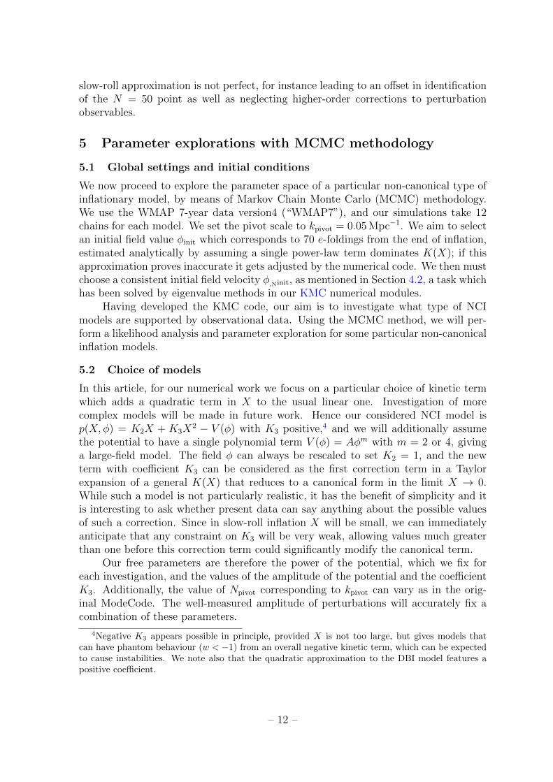
Figure 6. Parameter constraints for NCI model with quadratic potential. Left: Constraintson logm2 and K3 against Npivot for WMAP7 data. The countours are 68% (inner) and95% (outer) confidence levels, while the colour scale shows the sample mean likelihood inbins. Right: one-dimensional posterior distributions for the parameters (solid) and the meanlikelihoods (dashed).

imum likelihood values are given in Table 2, and the posterior distributions in Figures6 and 7.

The parameter of principal interest in each case is K3. In the quadratic potentialcase, this parameter turns out to be completely unconstrained by the data. This is tobe expected, as the quadratic potential gives acceptable observables when the kineticterm is either X or X2, which are the limits of small and large K3. The MCMC resultsshow that the fit to data remains acceptable right to the largest values of K3 that wepermit. We clearly see the two limiting behaviours of domination by either the X orX2 term; for example in the 2D m2–K3 constraint plot the former region has constantlogm2 ' −10, while the latter has K3 ∝ m4 as implied by taking constant Ps in thethird column of Table 1 to obtain the observed amplitude. The bimodal likelihood ofr is caused by the different values of this parameter in the two regimes. We also seea very mildly enhanced likelihood in the transition regime K3 ' 1012, but all valuesof K3 are acceptable Perhaps surprisingly, then, present data can say nothing about

Models Priors ns,ML rML −2 lnLML

(NCI) logA logK3

(1, 2; 2) (−16 ,−4) (0, 20) 0.965 0.080 7469.8(1, 2; 4) (−18 ,−4) (0, 20) 0.957 0.115 7471.8

Table 2. Priors for the parameters, logA and logK3, and the maximum likelihood (ML)values for ns and r from WMAP7. NCI models with single-term potentials provide a red tilt,ns < 1, and a detectable tensor-to-scalar ratio r ∼ 0.1.

– 14 –

Npivot

log

λ

40 45 50 55

−12

−11

−10

−9

−8

−7

−6

−5

−4

Npivot

log

k 3

40 45 50 55

11

12

13

14

15

16

17

18

19

20

log λ

log

k 3

−12 −8 −4

11

12

13

14

15

16

17

18

19

20

ns

r

0.94 0.945 0.95 0.955

0.115

0.12

0.125

0.13

0.135

0.14

0.145

0.15

0.155

0.16

0.165

−12.5−12−11.5−11−10.5−10−9.5−9−8.5−8−7.5−7−6.5−6−5.5−5−4.5−4log λ

11 12 13 14 15 16 17 18 19 20log k

3

0.94 0.945 0.95 0.955n

s

0.12 0.13 0.14 0.15 0.16r

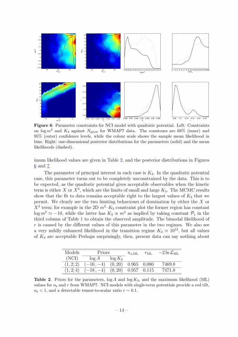
Figure 7. Parameter constraints for NCI model with single term quartic potential. Thisfigure uses the same convention as in figure 6.

the amplitude of a quadratic kinetic term added to the normal canonical one for thispotential, and as this is a potential known to fit the data well in the canonical case wecan conclude that more generally a quadratic correction term cannot be constraineddirectly from data.

The quartic potential case shown in Figure 7 is more interesting. In the standardcosmology, K3 → 0, the quartic potential is quite disfavoured by WMAP7. As wewould anticipate from the slow-roll results of Section 3, the situation for this potentialactually improves in the limit of large K3, as both ns and r move towards the scale-invariant values. Once more the MCMC results show that the fit remains good as thequadratic kinetic term becomes dominant and we find no observational upper limit onK3 for this potential. This time the distribution for r is unimodal, as only the X2

domination regime contributes to the posterior. There is a plausible non-zero lowerlimit on K3, though the numerical value of such a limit will be quite prior-dependent.Hence, incorporation of an X2 term is a method of salvaging the quartic model, thoughthe large value of K3, in Planck units, that is required is unattractive.

6 Conclusions

In this paper we introduced a numerical solver Kinetic Module Companions (KMC),an extension to ModeCode for a class of non-canonical inflation (NCI) models. In thisarticle we have used our code to investigate some simple non-canonical models, whichhave up to two terms in the kinetic energy and a monomial potential, in order to testthe validity of the code and provide some initial scientific results. We found that thesemodels are well able to fit current data, including in the quartic potential case pro-vided the quadratic kinetic term dominates. This is compatible with slow-roll resultswe obtained in the case of a single kinetic term of power-law form.

– 15 –

As a specific application of the code, we studied the introduction of a quadraticcorrection K3X

2 to the normal canonical kinetic term X, with the goal of constrainingthe coefficient K3. In practice, however, K3 turns out to be unconstrained by data,and indeed the inclusion of a large quadratic term can even improve the fit to WMAP7data, for instance for a quartic potential which, in the canonical case, is under severepressure from observations. Accordingly present data allow no leverage whatsoeveron radical deviations from the canonical case. In future work we plan a much morecomprehensive investigation of possible kinetic and potential forms.

A longer-term objective in this area may be to extend ModeCode to yet morecomplex forms of single scalar-field action, such as the Galileon [38] or indeed theHorndeski action [39] which is the most general scalar–tensor theory yielding second-order equations of motion. However the many functional degrees of freedom of suchactions will no doubt lead to considerable degeneracies given the relatively limitedamount of observational information available, which essentially amounts to only acouple of numbers at present. Hence, as we have found here even for the simplestseparable K-inflation case, one is likely to need considerable guidance from theory aswell as from observations in assessing whether the most general paradigms are useful.

Noted added: Shortly after we put this article on the arXiv, an independent paper[37] was submitted which contains results that partially overlap with ours.

Acknowledgments

S.L. was supported by a Sussex International Research Scholarship, and A.R.L. bythe Science and Technology Facilities Council [grant numbers ST/F002858/1 andST/I000976/1] and a Royal Society–Wolfson Research Merit Award. We thank theauthors of ModeCode for making their code public, and two of them, Richard Eastherand Hiranya Peiris, for discussions in relation to the work reported here. We alsothank Antony Lewis, David Seery and Wessel Valkenburg for useful discussions. Weacknowledge use of the Apollo HPC cluster at the University of Sussex and the SciamaHigh Performance Compute (HPC) cluster which is supported by the ICG, SEPnetand the University of Portsmouth.

References

[1] M. J. Mortonson, H. V. Peiris and R. Easther, Bayesian Analysis of Inflation:Parameter Estimation for Single Field Models, Phys. Rev. D 83, 043505 (2011)[arXiv:1007.4205 [astro-ph.CO]]. [The codes are publicly available at http://zuserver2.star.ucl.ac.uk/~hiranya/ModeCode/ModeCode/ModeCode.html]

[2] J. Dunkley et al. [WMAP Collaboration], Five-Year Wilkinson Microwave AnisotropyProbe (WMAP) Observations: Likelihoods and Parameters from the WMAP data,Astrophys. J. Suppl. 180, 306 (2009), [arXiv:0803.0586 [astro-ph]].

[3] E. Komatsu et al. [WMAP Collaboration], Five-Year Wilkinson Microwave AnisotropyProbe (WMAP) Observations: Cosmological Interpretation, Astrophys. J. Suppl. 180,330 (2009), [arXiv:0803.0547 [astro-ph]].

– 16 –

[4] E. Komatsu et al., Seven-year Wilkinson Microwave Anisotropy Probe (WMAP)observations: cosmological interpretation, Astrophys. J. Supp. 192, 18 (2011),[arXiv:1001.4538v2 [astro-ph.CO]].

[5] D. Larson, J. Dunkley, G. Hinshaw, E. Komatsu, M. R. Nolta, C. L. Bennett, B. Goldand M. Halpern et al., Seven-Year Wilkinson Microwave Anisotropy Probe (WMAP)Observations: Power Spectra and WMAP-Derived Parameters, Astrophys. J. Suppl.192, 16 (2011), [arXiv:1001.4635 [astro-ph.CO]].

[6] S. Dodelson, W. H. Kinney and E. W. Kolb, Cosmic microwave backgroundmeasurements can discriminate among inflation models, Phys. Rev. D 56, 3207 (1997),[astro-ph/9702166].

[7] W. H. Kinney, Inflation: Flow, fixed points and observables to arbitrary order in slowroll, Phys. Rev. D 66, 083508 (2002) [astro-ph/0206032].

[8] H. V. Peiris et al., First Year Wilkinson Microwave Anisotropy Probe (WMAP)Observations: Implications for Inflation, Astrophys. J. Supp. 148, 213 (2003)[astro-ph/0302225].

[9] S. Leach and A. R. Liddle, Constraining slow-roll inflation with WMAP and 2dF,Phys. Rev. D 68, 123508 (2003), [astro-ph/0306305].

[10] L. Alabidi and D. H. Lyth, Inflation models and observation, JCAP 0605, 016 (2006),[astro-ph/0510441].

[11] H. Peiris and R. Easther, Recovering the Inflationary Potential and Primordial PowerSpectrum With a Slow Roll Prior: Methodology and Application to WMAP 3 YearData, JCAP 0607, 002 (2006) [astro-ph/0603587].

[12] W. H. Kinney, E. W. Kolb, A. Melchiorri and A. Riotto, Inflation model constraintsfrom the Wilkinson Microwave Anisotropy Probe three-year data, Phys. Rev. D 74,023502 (2006) [astro-ph/0605338].

[13] C. Ringeval, The exact numerical treatment of inflationary models, Lect. Notes Phys.738, 243 (2008) [astro-ph/0703486].

[14] W. H. Kinney, E. W. Kolb, A. Melchiorri and A. Riotto, Latest inflation modelconstraints from cosmic microwave background measurements, Phys. Rev. D 78,087302 (2008) [arXiv:0805.2966 [astro-ph]].

[15] J. Hamann, J. Lesgourgues and W. Valkenburg, How to constrain inflationaryparameter space with minimal priors, JCAP 0804, 016 (2008) [arXiv:0802.0505[astro-ph]].

[16] P. Adshead and R. Easther, Constraining Inflation, JCAP 0810, 047 (2008)[arXiv:0802.3898 [astro-ph]].

[17] N. Agarwal and R. Bean, Cosmological constraints on general, single field inflation,Phys. Rev. D 79, 023503 (2009) [arXiv:0809.2798 [astro-ph]].

[18] A. Lewis, A. Challinor and A. Lasenby, Efficient Computation of CMB anisotropies inclosed FRW models, Astrophys. J. 538, 473 (2000), [astro-ph/9911177]. Code athttp://camb.info/

[19] A. Lewis and S. Bridle, Cosmological parameters from CMB and other data: A Monte

– 17 –

Carlo approach, Phys. Rev. D 66, 103511 (2002), [astro-ph/0205436]. Code athttp://cosmologist.info/cosmomc/

[20] A. D. Linde, A New Inflationary Universe Scenario: A Possible Solution Of TheHorizon, Flatness, Homogeneity, Isotropy And Primordial Monopole Problems, Phys.Lett. B 108, 389 (1982).

[21] A. D. Linde, Chaotic Inflation, Phys. Lett. B 129, 177 (1983).

[22] A. Sen, Rolling tachyon, JHEP 0204, 048 (2002), [hep-th/0203211].

[23] A. Sen, Tachyon matter, JHEP 0207, 065 (2002), [hep-th/0203265].

[24] N. C. Devi, A. Nautiyal and A. A. Sen, WMAP Constraints On K-Inflation, Phys.Rev. D 84, 103504 (2011), [arXiv:1107.4911 [astro-ph.CO]].

[25] L. Lorenz, J. Martin and C. Ringeval, Constraints on Kinetically Modified Inflationfrom WMAP5, Phys. Rev. D 78, 063543 (2008), [arXiv:0807.2414 [astro-ph]].

[26] C. Armendariz-Picon, T. Damour, V. F. Mukhanov, K-inflation, Phys. Lett. B458(1999) 209-218, [hep-th/9904075].

[27] J. Garriga, V. F. Mukhanov, Perturbations in k-inflation, Phys. Lett. B458 (1999)219-225, [hep-th/9904176].

[28] L. Lorenz, J. Martin and C. Ringeval, K-inflationary Power Spectra in the UniformApproximation, Phys. Rev. D 78, 083513 (2008), [arXiv:0807.3037 [astro-ph]].

[29] R. Easther and H. Peiris, Bayesian Analysis of Inflation II: Model Selection andConstraints on Reheating, arXiv:1112.0326 [astro-ph.CO].

[30] J. Norena, C. Wagner, L. Verde, H. V. Peiris and R. Easther, Bayesian Analysis ofInflation III: Slow Roll Reconstruction Using Model Selection, arXiv:1202.0304[astro-ph.CO].

[31] I. J. Grivell and A. R. Liddle, Accurate determination of inflationary perturbations,Phys. Rev. D54, 7191 (1996), [astro-ph/9607096].

[32] J. Martin and C. Ringeval, Inflation after WMAP3: Confronting the Slow-Roll andExact Power Spectra to CMB Data, JCAP 0608, 009 (2006), [astro-ph/0605367].

[33] J. Lesgourgues and W. Valkenburg, New constraints on the observable inflatonpotential from WMAP and SDSS, Phys. Rev. D 75, 123519 (2007), [astro-ph/0703625].

[34] J. Lesgourgues, A. A. Starobinsky and W. Valkenburg, What do WMAP and SDSSreally tell about inflation?, JCAP 0801, 010 (2008) [arXiv:0710.1630 [astro-ph]].

[35] F. Finelli, J. Hamann, S. M. Leach and J. Lesgourgues, Single-field inflationconstraints from CMB and SDSS data, JCAP 1004, 011 (2010) [arXiv:0912.0522[astro-ph.CO]].

[36] J. Martin, C. Ringeval and R. Trotta, Hunting Down the Best Model of Inflation withBayesian Evidence, Phys. Rev. D 83, 063524 (2011), [arXiv:1009.4157 [astro-ph.CO]].

[37] S. Unnikrishnan, V. Sahni and A. Toporensky, Refining inflation using non-canonicalscalars, arXiv:1205.0786 [astro-ph.CO].

[38] A. Nicolis, R. Rattazzi, and E. Trincherini, The galileon as a local modification ofgravity, Phys. Rev. D79, 064036 (2009) [arXiv:0811.2197 [hep-th]].

– 18 –

[39] G. W. Horndeski, Second-order scalar-tensor field equations in a four-dimensionalspace, Int. J. Theor. Phys. 10, 363 (1974).

– 19 –