Oboe: Collaborative Filtering for AutoML Model SelectionChengrun Yang, Yuji Akimoto, Dae Won Kim, Madeleine Udell

Cornell University{cy438,ya242,dk444,udell}@cornell.edu

ABSTRACT

Algorithm selection and hyperparameter tuning remain two of themost challenging tasks in machine learning. Automated machinelearning (AutoML) seeks to automate these tasks to enable wide-spread use of machine learning by non-experts. This paper intro-duces Oboe, a collaborative filtering method for time-constrainedmodel selection and hyperparameter tuning. Oboe forms a ma-trix of the cross-validated errors of a large number of supervisedlearning models (algorithms together with hyperparameters) ona large number of datasets, and fits a low rank model to learn thelow-dimensional feature vectors for the models and datasets thatbest predict the cross-validated errors. To find promising models fora new dataset, Oboe runs a set of fast but informative algorithmson the new dataset and uses their cross-validated errors to inferthe feature vector for the new dataset. Oboe can find good modelsunder constraints on the number of models fit or the total timebudget. To this end, this paper develops a new heuristic for activelearning in time-constrained matrix completion based on optimalexperiment design. Our experiments demonstrate that Oboe deliv-ers state-of-the-art performance faster than competing approacheson a test bed of supervised learning problems. Moreover, the suc-cess of the bilinear model used by Oboe suggests that AutoML maybe simpler than was previously understood.

KEYWORDS

AutoML, meta-learning, time-constrained, model selection, collabo-rative filtering

1 INTRODUCTION

It is often difficult to find the best algorithm and hyperparametersettings for a new dataset, even for experts in machine learningor data science. The large number of machine learning algorithmsand their sensitivity to hyperparameter values make it practicallyinfeasible to enumerate all configurations. Automated machinelearning (AutoML) seeks to efficiently automate the selection ofmodel (e.g., [8, 12, 14]) or pipeline (e.g., [11]) configurations, andhas become more important as the number of machine learningapplications increases.

We propose an algorithmic system, Oboe 1, that provides aninitial tuning for AutoML: it selects a good algorithm and hyperpa-rameter combination from a discrete set of options. The resultingmodel can be used directly, or the hyperparameters can be tunedfurther. Briefly, Oboe operates as follows.

During an offline training phase, it forms a matrix of the cross-validated errors of a large number of supervised-learning models(algorithms together with hyperparameters) on a large numberof datasets. It then fits a low rank model to this matrix to learnlatent low-dimensional meta-features for the models and datasets.1 The eponymous musical instrument plays the initial note to tune an orchestra.

Our optimization procedure ensures these latent meta-features bestpredict the cross-validated errors, among all bilinear models.

To find promising models for a new dataset, Oboe chooses a setof fast but informative models to run on the new dataset and usestheir cross-validated errors to infer the latent meta-features of thenew dataset. Given more time, Oboe repeats this procedure usinga higher rank to find higher-dimensional (and more expressive)latent features. Using a low rank model for the error matrix is avery strong structural prior.

This system addresses two important problems: 1) Time-constrainedinitialization: how to choose a promising initial model under timeconstraints. Oboe adapts easily to short times by using a very lowrank and by restricting its experiments to models that will runvery fast on the new dataset. 2) Active learning: how to improve onthe initial guess given further computational resources. Oboe usesextra time by allowing higher ranks and more expensive computa-tional experiments, accumulating its knowledge of the new datasetto produce more accurate (and higher-dimensional) estimates of itslatent meta-features.

Oboe uses collaborative filtering for AutoML, selecting modelsthat have worked well on similar datasets, as have many previousmethods including [1, 9, 12, 28, 38, 45]. In collaborative filtering,the critical question is how to characterize dataset similarity sothat training datasets “similar” to the test dataset faithfully predictmodel performance. One line of work uses dataset meta-features —simple, statistical or landmarking metrics — to characterize datasets[9, 12–14, 31]. Other approaches (e.g., [43]) avoid meta-features.Our approach builds on both of these lines of work. Oboe relieson model performance to characterize datasets, and the low rankrepresentations it learns for each dataset may be seen (and used) aslatent meta-features. Compared to AutoML systems that computemeta-features of the dataset before running any models, the flowof information in Oboe is exactly opposite: Oboe uses only theperformance of various models on the datasets to compute lowerdimensional latent meta-features for models and datasets.

The active learning subproblem is to gain the most informa-tion to guide further model selection. Some approaches choose afunction class to capture the dependence of model performanceon hyperparameters; examples are Gaussian processes [3, 14, 17,27, 33, 34, 36, 37], sparse Boolean functions [16] and decision trees[2, 20]. Oboe chooses the set of bilinear models as its function class:predicted performance is linear in each of the latent model anddataset meta-features.

Bilinearity seems like a rather strong assumption, but confersseveral advantages. Computations are fast and easy: we can findthe global minimizer by PCA, and can infer the latent meta-featuresfor a new dataset using least squares. Moreover, recent theoreticalwork suggests that this model class is more general than it appears:roughly, and under a few mild technical assumptions, anym × n

arX

iv:1

808.

0323

3v2

[cs

.LG

] 2

0 M

ay 2

019

Training

Validation

Test

Learning

(a) Learning

Training

Validation

Test

Learning

Training

Meta­learning

Validation

Test

Training

Validation

Test

Meta­training

       

Meta­validation

Meta­test

(b) Meta-learning

Figure 1: Standard vs meta-learning.

matrix with independent rows and columns whose entries are gen-erated according to a fixed function (here, the function computedby training the model on the dataset) has an approximate rank thatgrows as log(m + n) [40]. Hence large data matrices tend to looklow rank.

Originally, the authors conceived of Oboe as a system to producea good set of initial models, to be refined by other local search meth-ods, such as Bayesian optimization. However, in our experiments,we find that Oboe’s performance, refined by fitting models of everhigher rank with ever more data, actually improves faster thancompeting methods that use local search methods more heavily.

One key component of our system is the prediction of modelruntime on new datasets. Many authors have previously studiedalgorithm runtime prediction using a variety dataset features [21],via ridge regression [18], neural networks [35], Gaussian processes[19], and more. Several measures have been proposed to trade-off between accuracy and runtime [4, 25]. We predict algorithmruntime using only the number of samples and features in thedataset. This model is particularly simple but surprisingly effective.

Classical experiment design (ED) [5, 22, 29, 32, 42] selects fea-tures to observe to minimize the variance of the parameter esti-mate, assuming that features depend on the parameters accordingto known, linear, functions. Oboe’s bilinear model fits this para-digm, and so ED can be used to select informative models. Budgetconstraints can be added, as we do here, to select a small numberof promising machine learning models or a set predicted to finishwithin a short time budget [24, 46].

This paper is organized as follows. Section 2 introduces notationand terminology. Section 3 describes the main ideas we use in Oboe.Section 4 presents Oboe in detail. Section 5 shows experiments.

2 NOTATION AND TERMINOLOGY

Meta-learning. Meta-learning is the process of learning acrossindividual datasets or problems, which are subsystems on whichstandard learning is performed [26]. Just as standard machine learn-ing must avoid overfitting, experiments testing AutoML systemsmust avoid meta-overfitting! We divide our set of datasets intometa-training, meta-validation and meta-test sets, and report re-sults on the meta-test set. Each of the three phases in meta-learning— meta-training, meta-validation and meta-test — is a standardlearning process that includes training, validation and test.Indexing. Throughout this paper, all vectors are column vectors.Given a matrix A ∈ Rm×n , Ai, : and A:, j denote the ith row and jthcolumn of A, respectively. i is the index over datasets, and j is the

index over models. We define [n] = {1, . . . ,n} for n ∈ Z. Given anordered set S = {s1, . . . , sk } where s1 < . . . < sk ∈ [n], we writeA:S =

[A:,s1 A:,s2 · · · A:,sk

].

Algorithm performance. A model A is a specific algorithm-hyperparameter combination, e.g. k-NN with k = 3. We denote byA(D) the expected cross-validation error of modelA on datasetD,where the expectation is with respect to the cross-validation splits.We refer to the model in our collection that achieves minimal erroron D as the best model for D. A model A is said to be observedon D if we have calculated A(D) by fitting (and cross-validating)the model. The performance vector e of a dataset D concatenatesA(D) for each model A in our collection.Meta-features. We discuss two types of meta-features in this pa-per. Meta-features refer to metrics used to characterize datasets ormodels. For example, the number of data points or the performanceof simple models on a dataset can serve as meta-features of thedataset. As an example, we list the meta-features used in the Au-toML framework auto-sklearn in Appendix B, Table 3. In constrastto standard meta-features, we use the term latent meta-features torefer to characterizations learned from matrix factorization.Parametric hierarchy. We distinguish between three kinds ofparameters:• Parameters of a model (e.g., the splits in a decision tree) areobtained by training the model.• Hyperparameters of an algorithm (e.g., the maximum depthof a decision tree) govern the training procedure. We usethe word model to refer to an algorithm together with aparticular choice of hyperparameters.• Hyper-hyperparameters of a meta-learning method (e.g., thetotal time budget for Oboe) govern meta-training.

Time target and time budget. The time target refers to the an-ticipated time spent running models to infer latent features of eachfixed dimension and can be exceeded. However, the runtime doesnot usually deviate much from the target since our model runtimeprediction works well. The time budget refers to the total time limitfor Oboe and is never exceeded.MidsizeOpenMLandUCI datasets. Our experiments useOpenML[41] and UCI [10] classification datasets with between 150 and10,000 data points and with no missing entries.

3 METHODOLOGY

3.1 Model Performance Prediction

It can be difficult to determine a priori which meta-features to useso that algorithms perform similarly well on datasets with similarmeta-features. Also, the computation of meta-features can be ex-pensive (see Appendix C, Figure 11). To infer model performanceon a dataset without any expensive meta-feature calculations, weuse collaborative filtering to infer latent meta-features for datasets.

As shown in Figure 2, we construct an empirical error matrixE ∈ Rm×n , where every entry Ei j records the cross-validated er-ror of model j on dataset i . Empirically, E has approximately lowrank: Figure 3 shows the singular values σi (E) decay rapidly as afunction of the index i . This observation serves as foundation ofour algorithm, and will be analyzed in greater detail in Section 5.2.The value Ei j provides a noisy but unbiased estimate of the trueperformance of a model on the dataset: EEi j = Aj (Di ).

2

PCA

impute(white entries)

models

datasets

dataset latent meta­features

datasets 

 

models

model latent meta­features

XT Y E 

Figure 2: Illustration of model performance prediction via

the error matrix E (yellow blocks only). Perform PCA on

the error matrix (offline) to compute dataset (X ) and model

(Y ) latentmeta-features (orange blocks). Given a newdataset

(row with white and blue blocks), pick a subset of models to

observe (blue blocks). UseY together with the observedmod-

els to impute the performance of the unobserved models on

the new dataset (white blocks).

0 10 20 30 40 50index i

100

101

102

103

104

105

σi

Figure 3: Singular value decay of an errormatrix. The entries

are calculated by 5-fold cross validation of machine models

(listed in Appendix A, Table 2) onmidsize OpenML datasets.

To denoise this estimate, we approximate Ei j ≈ x⊤i yj wherexi and yj minimize

∑mi=1

∑nj=1(Ei j − x⊤i yj )

2 with xi ,yj ∈ Rk fori ∈ [M] and j ∈ [N ]; the solution is given by PCA. Thus xi andyj arethe latent meta-features of dataset i and model j, respectively. Therank k controls model fidelity: small ks give coarse approximations,while large ks may overfit. We use a doubling scheme to choose kwithin time budget; see Section 4.2 for details.

Given a new meta-test dataset, we choose a subset S ⊆ [N ] ofmodels and observe performance ej of model j for each j ∈ S. Agood choice of S balances information gain against time needed torun the models; we discuss how to choose S in Section 3.3. We theninfer latent meta-features for the new dataset by solving the leastsquares problem: minimize

∑j ∈S(ej − x⊤yj )2 with x ∈ Rk . For all

unobserved models, we predict their performance as ej = x⊤yj forj < S.

3.2 Runtime Prediction

Estimating model runtime allows us to trade off between runningslow, informative models and fast, less informative models. We usea simple method to estimate runtimes, using polynomial regressionon nD and pD , the numbers of data points and features in D,and their logarithms, since the theoretical complexities of machinelearning algorithmswe use areO

((nD )3, (pD )3, (log(nD ))3

). Hence

we fit an independent polynomial regression model for each model:

fj = argminfj ∈FM∑i=1

(fj (nDi ,pDi , log(nDi )) − tDi

j

)2, j ∈ [n]

where tDj is the runtime of machine learning model j on datasetD, and F is the set of all polynomials of order no more than 3. Wedenote this procedure by fj = fit_runtime(n,p, t).

We observe that this model predicts runtime within a factor oftwo for half of the machine learning models on more than 75%midsize OpenML datasets, and within a factor of four for nearly allmodels, as shown in Section 5.2 and visualized in Figure 7.

3.3 Time-Constrained Information Gathering

To select a subset S of models to observe, we adopt an approachthat builds on classical experiment design: we suppose fitting eachmachine learning model j ∈ [n] returns a linear measurement xTyjof x , corrupted by Gaussian noise. To estimate x , we would liketo choose a set of observations yj that span Rk and form a well-conditioned submatrix, but that corresponds to models which arefast to run. In passing, we note that the pivoted QR algorithm on thematrix Y (heuristically) finds a well conditioned set of k columns ofY . However, we would like to find a method that is runtime-aware.

Our experiment design (ED) procedure minimizes a scalarizationof the covariance of the estimatedmeta-features x of the new datasetsubject to runtime constraints [5, 22, 29, 32, 42]. Formally, definean indicator vector v ∈ {0, 1}n , where entry vj indicates whetherto fit model j. Let tj denote the predicted runtime of model j ona meta-test dataset, and let yj denote its latent meta-features, forj ∈ [n]. Now relax to allow v ∈ [0, 1]n to allow for non-Booleanvalues and solve the optimization problem

minimize log det( ∑n

j=1vjyjy⊤j

)−1subject to

n∑j=1

vj tj ≤ τ

vj ∈ [0, 1],∀j ∈ [n](1)

with variable v ∈ Rn . We call this method ED (time). Scalarizingthe covariance by minimizing the determinant is called D-optimaldesign. Several other scalarizations can also be used, includingcovariance norm (E-optimal) or trace (A-optimal). Replacing ti by 1gives an alternative heuristic that bounds the number of models fitby τ ; we call this method ED (number).

Problem 1 is a convex optimization problem, and we obtain anapproximate solution by rounding the largest entries of v up to1 until the selected models exceed the time limit τ . Let S ⊆ [n]be the set of indices of e that we choose to observe, i.e. the setsuch that vs rounds to 1 for s ∈ S. We denote this process byS = min_variance_ED(t , {yj }nj=1,τ ).

4 THE OBOE SYSTEM

Shown in Figure 4, the Oboe system can be divided into offline andonline stages. The offline stage is executed only once and exploresthe space of model performance on meta-training datasets. Timetaken on this stage does not affect the runtime of Oboe on a newdataset; the runtime experienced by user is that of the online stage.

3

datapreprocessing

error matrixgeneration

compute lowdimensionalalgorithmfeatures

time­constrainedmodel selection

inferperformance ofother models

ensemblingdatapreprocessing

offline stage

time target doubling

                         time­constrained online stage

training datasets

test dataset predictions

timeremains?

Yes

No

Figure 4: Diagram of data processing flow in the Oboe system.

One advantage of Oboe is that the vast majority of the timein the online phase is spent training standard machine learningmodels, while very little time is required to decide which models tosample. Training these standard machine learning models requiresrunning algorithms on datasets with thousands of data points andfeatures, while the meta-learning task — deciding which models tosample — requires only solving a small least-squares problem.

4.1 Offline Stage

The (i, j)th entry of error matrix E ∈ Rm×n , denoted as Ei j , recordsthe performance of the jth model on the ith meta-training dataset.We generate the error matrix using the balanced error rate met-ric, the average of false positive and false negative rates acrossdifferent classes. At the same time we record runtime of machinelearning models on datasets. This is used to fit runtime predictorsdescribed in Section 3. Pseudocode for the offline stage is shown asAlgorithm 1.

Algorithm 1 Offline StageRequire: meta-training datasets {Di }mi=1, models {Aj }nj=1, algo-

rithm performance metricMEnsure: error matrix E, runtimematrixT , fitted runtime predictors{ fj }nj=1

1: for i = 1, 2, . . . ,m do

2: nDi ,pDi ← number of data points and features in Di3: for j = 1, 2, . . . ,n do

4: Ei j ← error of model Aj on dataset Di according tometricM

5: Ti j ← observed runtime for model Aj on dataset Di6: end for

7: end for

8: for j = 1, 2, . . . ,n do

9: fit fj = fit_runtime(n,p,Tj )10: end for

4.2 Online Stage

Recall that we repeatly double the time target of each round until weuse up the total time budget. Thus each round is a subroutine of theentire online stage and is shown as Algorithm 2, fit_one_round.

• Time-constrained model selection (fit_one_round) Our ac-tive learning procedure selects a fast and informative collectionof models to run on the meta-test dataset. Oboe uses the resultsof these fits to estimate the performance of all other models asaccurately as possible. The procedure is as follows. First pre-dict model runtime on the meta-test dataset using fitted runtimepredictors. Then use experiment design to select a subset S ofentries of e , the performance vector of the test dataset, to observe.The observed entries are used to compute x , an estimate of thelatent meta-features of the test dataset, which in turn is used topredict every entry of e . We build an ensemble out of modelspredicted to perform well within the time target τ by means ofgreedy forward selection [6, 7]. We denote this subroutine asA =ensemble_selection(S, eS , zS), which takes as input theset of base learners S with their cross-validation errors eS andpredicted labels zS = {zs |s ∈ S}, and outputs ensemble learnerA. The hyperparameters used by models in the ensemble canbe tuned further, but in our experiments we did not observesubstantial improvements from further hyperparameter tuning.• Time target doubling To select rank k ,Oboe starts with a smallinitial rank along with a small time target, and then doubles thetime target for fit_one_round until the elapsed time reacheshalf of the total budget. The rank k increments by 1 if the valida-tion error of the ensemble learner decreases after doubling thetime target, and otherwise does not change. Since the matricesreturned by PCA with rank k are submatrices of those returnedby PCA with rank l for l > k , we can compute the factors assubmatrices of the m-by-n matrices returned by PCA with fullrank min(m,n) [15]. The pseudocode is shown as Algorithm 3.

4

Algorithm 2 fit_one_round({yj }nj=1, { fj }nj=1,Dtr , τ )

Require: model latent meta-features {yj }nj=1, fitted runtime pre-dictors { fj }nj=1, training fold of the meta-test datasetDtr, num-ber of best models N to select from the estimated performancevector, time target for this round τ

Ensure: ensemble learner A1: for j = 1, 2, . . . ,n do

2: tj ← fj (nDtr ,pDtr )3: end for

4: S = min_variance_ED(t , {yj }nj=1, τ )5: for k = 1, 2, . . . , |S| do6: eSk ← cross-validation error of model ASk on Dtr7: end for

8: x ← ([yS1 yS2 · · · yS|S|

]⊤)†eS

9: e ←[y1 y2 · · · yn

]⊤x

10: T ← the N models with lowest predicted errors in e11: for k = 1, 2, . . . , |T | do12: eTk , zTk ← cross-validation error of model ATk on Dtr13: end for

14: A←ensemble_selection(T , eT , zT )

Algorithm 3 Online StageRequire: error matrix E, runtime matrix T , meta-test dataset D,

total time budget τ , fitted runtime predictors { fj }nj=1, initialtime target τ0, initial approximate rank k0

Ensure: ensemble learner A1: xi ,yj ← argmin

∑mi=1

∑nj=1(Ei j − x⊤i yj )

2, xi ∈ Rmin(m,n) fori ∈ [M] , yj ∈ Rmin(m,n) for j ∈ [N ]

2: Dtr,Dval,Dte ← training, validation and test folds of D3: τ ← τ04: k ← k05: while τ ≤ τ/2 do6: {yj }nj=1 ← k-dimensional subvectors of {yj }nj=17: A← fit_one_round({yj }nj=1, { fj }

nj=1,Dtr, τ )

8: e ′A← A(Dval)

9: if e ′A< eA then

10: k ← k + 111: end if

12: τ ← 2τ13: eA ← e ′

A14: end while

5 EXPERIMENTAL EVALUATION

We ran all experiments on a server with 128 Intel® Xeon® E7-4850v4 2.10GHz CPU cores. The process of running each system ona specific dataset is limited to a single CPU core. Code for theOboe system is at https://github.com/udellgroup/oboe; code forexperiments is at https://github.com/udellgroup/oboe-testing.

We test different AutoML systems on midsize OpenML and UCIdatasets, using standard machine learning models shown in Ap-pendix A, Table 2. Since data pre-processing is not our focus, we

pre-process all datasets in the same way: one-hot encode categor-ical features and then standardize all features to have zero meanand unit variance. These pre-processed datasets are used in all theexperiments.

5.1 Performance Comparison across AutoML

Systems

We compare AutoML systems that are able to select among differentalgorithm types under time constraints: Oboe (with error matrixgenerated from midsize OpenML datasets), auto-sklearn [12], prob-abilistic matrix factorization (PMF) [14], and a time-constrainedrandom baseline. The time-constrained random baseline selectsmodels to observe randomly from those predicted to take less timethan the remaining time budget until the time limit is reached.

5.1.1 Comparison with PMF. PMF and Oboe differ in the surrogatemodels they use to explore the model space: PMF incrementallypicks models to observe using Bayesian optimization, with modellatent meta-features from probabilistic matrix factorization as fea-tures, while Oboe models algorithm performance as bilinear inmodel and dataset meta-features.

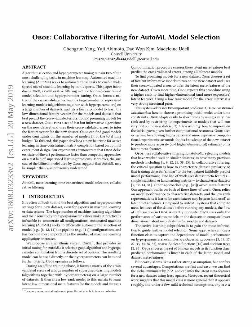
PMF does not limit runtime, hence we compare it to Oboe us-ing either QR or ED (number) to decide the set S of models (seeSection 3.3). Figure 5 compares the performance of PMF and Oboe(using QR and ED (number) to decide the set S of models) on ourcollected error matrix to see which is best able to predict the small-est entry in each row. We show the regret: the difference betweenthe minimal entry in each row and the one found by the AutoMLmethod. In PMF,N0 = 5models are chosen from the best algorithmson similar datasets (according to dataset meta-features shown inAppendix B, Table 3) are used to warm-start Bayesian optimization,which then searches for the next model to observe. Oboe does notrequire this initial information before beginning its exploration.However, for a fair comparison, we show both "warm" and "cold"versions. The warm version observes both the models chosen bymeta-features and those chosen by QR or ED; the number of ob-served entries in Figure 5 is the sum of all observed models. Thecold version starts from scratch and only observes models chosenby QR and ED.

(Standard ED also performs well; see Appendix D, Figure 12.)Figure 5 shows the surprising effectiveness of the low rankmodel

used by Oboe:1 Meta-features are of marginal value in choosing new models toobserve. For QR, using models chosen by meta-features helps whenthe number of observed entries is small. For ED, there is no benefitto using models chosen by meta-features.2 The low rank structure used by QR and ED seems to provide abetter guide to which models will be informative than the Gaussianprocess prior used by PMF: the regret of PMF does not decrease asfast as Oboe using either QR or ED.

5.1.2 Comparison with auto-sklearn. The comparison with PMFassumes we can use the labels for every point in the entire datasetfor model selection, so we can compare the performance of everymodel selected and pick the one with lowest error. In contrast, ourcomparison with auto-sklearn takes place in a more challenging, re-alistic setting: when doing cross-validation on the meta-test dataset,

5

5(2%) 15(6%) 25(11%) 35(15%)number (percentage) of observed entries

0.000

0.005

0.010

0.015

0.020

0.025

0.030

0.035

regr

et(m

ean±

stan

dar

der

ror)

5(2%) 15(6%) 25(11%) 35(15%)number (percentage) of observed entries

1.5

2.0

2.5

3.0

3.5

4.0

ran

k(m

ean±

stan

dar

der

ror)

5(2%) 15(6%) 25(11%) 35(15%)number (percentage) of observed entries

1.5

2.0

2.5

3.0

3.5

4.0

aver

age

rank

ED (number)

ED (number) with meta-features

PMF

QR

QR with meta-features

Figure 5: Comparison of sampling schemes (QR or ED) in

Oboe and PMF. "QR" denotes QR decomposition with col-

umn pivoting; "ED (number)" denotes experiment design

with number of observed entries constrained. The left plot

shows the regret of each AutoML method as a function of

number of entries; the right shows the relative rank of each

AutoML method in the regret plot (1 is best and 5 is worst).

we do not know the labels of the validation fold until we evaluateperformance of the ensemble we built within time constraints onthe training fold.

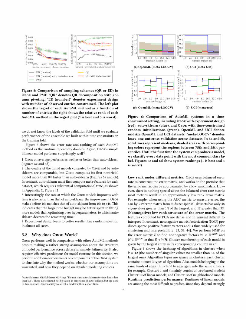
Figure 6 shows the error rate and ranking of each AutoMLmethod as the runtime repeatedly doubles. Again, Oboe’s simplebilinear model performs surprisingly well’2:1 Oboe on average performs as well as or better than auto-sklearn(Figures 6c and 6d).2 The quality of the initial models computed by Oboe and by auto-sklearn are comparable, but Oboe computes its first nontrivialmodel more than 8× faster than auto-sklearn (Figures 6a and 6b).In contrast, auto-sklearn must first compute meta-features for eachdataset, which requires substantial computational time, as shownin Appendix C, Figure 11.3 Interestingly, the rate at which the Oboe models improves withtime is also faster than that of auto-sklearn: the improvement Oboemakes before 16s matches that of auto-sklearn from 16s to 64s. Thisindicates that the large time budget may be better spent in fittingmore models than optimizing over hyperparameters, to which auto-sklearn devotes the remaining time.4 Experiment design leads to better results than random selectionin almost all cases.

5.2 Why does OboeWork?

Oboe performs well in comparison with other AutoML methodsdespite making a rather strong assumption about the structureof model performance across datasets: namely, bilinearity. It alsorequires effective predictions for model runtime. In this section, weperform additional experiments on components of theOboe systemto elucidate why the method works, whether our assumptions arewarranted, and how they depend on detailed modeling choices.

2Auto-sklearn’s GitHub Issue #537 says “Do not start auto-sklearn for time limits lessthan 60s". These plots should not be taken as criticisms of auto-sklearn, but are usedto demonstrate Oboe’s ability to select a model within a short time.

1.0 2.0 4.0 8.0 16.0 32.0 64.0runtime budget (s)

0.1

0.2

0.3

0.4

0.5

bal

ance

der

ror

rate

(a) OpenML (meta-LOOCV)

1.0 2.0 4.0 8.0 16.0 32.0 64.0runtime budget (s)

0.0

0.1

0.2

0.3

0.4

0.5

bal

ance

der

ror

rate

(b) UCI (meta-test)

1.0 2.0 4.0 8.0 16.0 32.0 64.0runtime budget (s)

1.8

1.9

2.0

2.1

2.2

ran

k(m

ean±

stan

dar

der

ror)

(c) OpenML (meta-LOOCV)

1.0 2.0 4.0 8.0 16.0 32.0 64.0runtime budget (s)

1.41.61.82.02.22.42.6

ran

k(m

ean±

stan

dar

der

ror)

(d) UCI (meta-test)

Figure 6: Comparison of AutoML systems in a time-

constrained setting, includingOboewith experiment design

(red), auto-sklearn (blue), and Oboe with time-constrained

random initializations (green). OpenML and UCI denote

midsize OpenML and UCI datasets. "meta-LOOCV" denotes

leave-one-out cross-validation across datasets. In 6a and 6b,

solid lines representmedians; shaded areaswith correspond-

ing colors represent the regions between 75th and 25th per-

centiles. Until the first time the system can produce amodel,

we classify every data point with the most common class la-

bel. Figures 6c and 6d show system rankings (1 is best and 3

is worst).

Low rank under different metrics. Oboe uses balanced errorrate to construct the error matrix, and works on the premise thatthe error matrix can be approximated by a low rank matrix. How-ever, there is nothing special about the balanced error rate metric:most metrics result in an approximately low rank error matrix.For example, when using the AUC metric to measure error, the418-by-219 error matrix from midsize OpenML datasets has only 38eigenvalues greater than 1% of the largest, and 12 greater than 3%.(Nonnegative) low rank structure of the error matrix. Thefeatures computed by PCA are dense and in general difficult tointerpret. In contrast, nonnegative matrix factorization (NMF) pro-duces sparse positive feature vectors and is thus widely used forclustering and interpretability [23, 39, 44]. We perform NMF onthe error matrix E to find nonnegative factors W ∈ Rm×k andH ∈ Rk×n so that E ≈WH . Cluster membership of each model isgiven by the largest entry in its corresponding column in H .

Figure 8 shows the heatmap of algorithms in clusters whenk = 12 (the number of singular values no smaller than 3% of thelargest one). Algorithm types are sparse in clusters: each clustercontains at most 3 types of algorithm. Also, models belonging to thesame kinds of algorithms tend to aggregate into the same clusters:for example, Clusters 1 and 4 mainly consist of tree-based models;Cluster 10 of linear models; and Cluster 12 of neighborhood models.Runtime prediction performance. Runtimes of linear modelsare among the most difficult to predict, since they depend strongly

6

Figure 7: Runtime prediction performance on different machine learning algorithms, on midsize OpenML datasets.

7

Dec

isio

nT

ree

Extr

aT

rees

Ran

dom

For

est

Gra

die

nt

Boos

tin

gG

auss

ian

Nai

veB

ayes

Ad

aboos

tK

ern

elS

VM

Lin

ear

SV

ML

ogis

tic

Reg

ress

ion

Per

cep

tron

Mu

ltil

ayer

Per

cep

tron

kN

N

123456789

101112

clu

ster

ind

ex

0

5

10

15

20

25

30

Figure 8: Algorithm heatmap in clusters. Each block is col-

ored by the number of models of the corresponding algo-

rithm type in that cluster. Numbers next to the scale bar re-

fer to the numbers of models.

Table 1: Runtime prediction accuracy on OpenML datasets

Algorithm type Runtime prediction accuracywithin factor of 2 within factor of 4

Adaboost 83.6% 94.3%Decision tree 76.7% 88.1%Extra trees 96.6% 99.5%Gradient boosting 53.9% 84.3%Gaussian naive Bayes 89.6% 96.7%kNN 85.2% 88.2%Logistic regression 41.1% 76.0%Multilayer perceptron 78.9% 96.0%Perceptron 75.4% 94.3%Random Forest 94.4% 98.2%Kernel SVM 59.9% 86.7%Linear SVM 30.1% 73.2%

on the conditioning of the problem. Our runtime prediction ac-curacy on midsize OpenML datasets is shown in Table 1 and inFigure 7. We can see that our empirical prediction of model run-time is roughly unbiased. Thus the sum of predicted runtimes onmultiple models is a roughly good estimate.Cold-start. Oboe uses D-optimal experiment design to cold-startmodel selection. In Figure 9, we compare this choice with A- andE-optimal design and nonlinear regression in Alors [28], by meansof leave-one-out cross-validation on midsize OpenML datasets. Wemeasure performance by the relative RMSE ∥e − e ∥2/∥e ∥2 of thepredicted performance vector and by the number of correctly pre-dicted best models, both averaged across datasets. The approximaterank of the error matrix is set to be the number of eigenvalues

2 4 6 8 10number of best entries

0%5%

10%15%20%25%30%35%

accu

racy

per

cent

age

(mea

n±

stan

dar

der

ror)

D-optimal

A-optimal

E-optimal

Alors

Figure 9: Comparison of

cold-start methods.

0 5 10 15 20 25number of models in ensemble

0%

10%

20%

30%

40%

rati

o

Figure 10: Histogram of

Oboe ensemble size. The

ensembles were built in exe-

cutions on midsize OpenML

datasets in Section 5.1.2.

larger than 1% of the largest, which is 38 here. The time limitin experiment design implementation is set to be 4 seconds; thenonlinear regressor used in Alors implementation is the defaultRandomForestRegressor in scikit-learn 0.19.2 [30].

The horizontal axis is the number of models selected; the verti-cal axis is the percentage of best-ranked models shared betweentrue and predicted performance vectors. D-optimal design robustlyoutperforms.Ensemble size. As shown in Figure 10, more than 70% of theensembles constructed on midsize OpenML datasets have no morethan 5 base learners. This parsimony makes our ensembles easy toimplement and interpret.

6 SUMMARY

Oboe is an AutoML system that uses collaborative filtering andoptimal experiment design to predict performance of machine learn-ing models. By fitting a few models on the meta-test dataset, thissystem transfers knowledge from meta-training datasets to select apromising set of models.Oboe naturally handles different algorithmand hyperparameter types and can match state-of-the-art perfor-mance of AutoML systems much more quickly than competingapproaches.

This work demonstrates the promise of collaborative filteringapproaches to AutoML. However, there is much more left to do.Future work is needed to adapt Oboe to different loss metrics, bud-get types, sparsely observed error matrices, and a wider range ofmachine learning algorithms. Adapting a collaborative filteringapproach to search for good machine learning pipelines, rather thanindividual algorithms, presents a more substantial challenge. Wealso hope to see more approaches to the challenge of choosinghyper-hyperparameter settings subject to limited computation anddata: meta-learning is generally data(set)-constrained. With con-tinuing efforts by the AutoML community, we look forward to aworld in which domain experts seeking to use machine learningcan focus on data quality and problem formulation, rather than ontasks — such as algorithm selection and hyperparameter tuning —which are suitable for automation.

ACKNOWLEDGMENTS

This work was supported in part by DARPA Award FA8750-17-2-0101. The authors thank Christophe Giraud-Carrier, Ameet Tal-walkar, Raul Astudillo Marban, Matthew Zalesak, Lijun Ding and

8

Davis Wertheimer for helpful discussions, thank Jack Dunn for ascript to parse UCI Machine Learning Repository datasets, and alsothank several anonymous reviewers for useful comments.

REFERENCES

[1] Rémi Bardenet, Mátyás Brendel, Balázs Kégl, and Michele Sebag. 2013. Collabo-rative hyperparameter tuning. In ICML. 199–207.

[2] Thomas Bartz-Beielstein and Sandor Markon. 2004. Tuning search algorithmsfor real-world applications: A regression tree based approach. In Congress onEvolutionary Computation, Vol. 1. IEEE, 1111–1118.

[3] James S Bergstra, Rémi Bardenet, Yoshua Bengio, and Balázs Kégl. 2011. Al-gorithms for hyper-parameter optimization. In Advances in Neural InformationProcessing Systems. 2546–2554.

[4] Bernd Bischl, Jakob Richter, Jakob Bossek, Daniel Horn, Janek Thomas, andMichelLang. 2017. mlrMBO: A modular framework for model-based optimization ofexpensive black-box functions. arXiv preprint arXiv:1703.03373 (2017).

[5] Stephen Boyd and Lieven Vandenberghe. 2004. Convex optimization. CambridgeUniversity Press.

[6] Rich Caruana, Art Munson, and Alexandru Niculescu-Mizil. 2006. Getting themost out of ensemble selection. In ICDM. IEEE, 828–833.

[7] Rich Caruana, Alexandru Niculescu-Mizil, Geoff Crew, and Alex Ksikes. 2004.Ensemble selection from libraries of models. In ICML. ACM, 18.

[8] Boyuan Chen, Harvey Wu, Warren Mo, Ishanu Chattopadhyay, and Hod Lipson.2018. Autostacker: A compositional evolutionary learning system. In Proceedingsof the Genetic and Evolutionary Computation Conference. ACM, 402–409.

[9] Tiago Cunha, Carlos Soares, and André C. P. L. F. de Carvalho. 2018. CF4CF:Recommending Collaborative Filtering Algorithms Using Collaborative Filtering.In Proceedings of the 12th ACM Conference on Recommender Systems (RecSys ’18).ACM, New York, NY, USA, 357–361. https://doi.org/10.1145/3240323.3240378

[10] Dua Dheeru and Efi Karra Taniskidou. 2017. UCI Machine Learning Repository.http://archive.ics.uci.edu/ml

[11] Iddo Drori, Yamuna Krishnamurthy, Remi Rampin, Raoni de Paula Lourenco,Jorge Piazentin Ono, Kyunghyun Cho, Claudio Silva, and Juliana Freire. 2018.AlphaD3M: Machine learning pipeline synthesis. In AutoML Workshop at ICML.

[12] Matthias Feurer, Aaron Klein, Katharina Eggensperger, Jost Springenberg, ManuelBlum, and Frank Hutter. 2015. Efficient and robust automated machine learning.In Advances in Neural Information Processing Systems. 2962–2970.

[13] Matthias Feurer, Jost Tobias Springenberg, and Frank Hutter. 2014. Using meta-learning to initialize Bayesian optimization of hyperparameters. In InternationalConference on Meta-learning and Algorithm Selection. Citeseer, 3–10.

[14] Nicolo Fusi, Rishit Sheth, andMelih Elibol. 2018. Probabilistic matrix factorizationfor automated machine learning. In Advances in Neural Information ProcessingSystems. 3352–3361.

[15] Gene H Golub and Charles F Van Loan. 2012. Matrix computations. JHU Press.[16] Elad Hazan, Adam Klivans, and Yang Yuan. 2018. Hyperparameter optimization:

a spectral approach. In ICLR. https://openreview.net/forum?id=H1zriGeCZ[17] Ralf Herbrich, Neil D Lawrence, and Matthias Seeger. 2003. Fast sparse Gauss-

ian process methods: The informative vector machine. In Advances in NeuralInformation Processing Systems. 625–632.

[18] Ling Huang, Jinzhu Jia, Bin Yu, Byung-Gon Chun, Petros Maniatis, and MayurNaik. 2010. Predicting execution time of computer programs using sparse polyno-mial regression. In Advances in Neural Information Processing Systems. 883–891.

[19] Frank Hutter, Youssef Hamadi, Holger H Hoos, and Kevin Leyton-Brown. 2006.Performance prediction and automated tuning of randomized and parametricalgorithms. In International Conference on Principles and Practice of ConstraintProgramming. Springer, 213–228.

[20] Frank Hutter, Holger H Hoos, and Kevin Leyton-Brown. 2011. Sequential Model-Based Optimization for General Algorithm Configuration. LION 5 (2011), 507–523.

[21] Frank Hutter, Lin Xu, Holger H Hoos, and Kevin Leyton-Brown. 2014. Algorithmruntime prediction: Methods & evaluation. Artificial Intelligence 206 (2014),79–111.

[22] RC St John and Norman R Draper. 1975. D-optimality for regression designs: areview. Technometrics 17, 1 (1975), 15–23.

[23] Jingu Kim and Haesun Park. 2008. Sparse nonnegative matrix factorization forclustering. Technical Report. Georgia Institute of Technology.

[24] Andreas Krause, Ajit Singh, and Carlos Guestrin. 2008. Near-optimal sensorplacements in Gaussian processes: Theory, efficient algorithms and empiricalstudies. Journal of Machine Learning Research 9, Feb (2008), 235–284.

[25] Rui Leite, Pavel Brazdil, and Joaquin Vanschoren. 2012. Selecting classificationalgorithms with active testing. In International Workshop on Machine Learningand Data Mining in Pattern Recognition. Springer, 117–131.

[26] Christiane Lemke, Marcin Budka, and Bogdan Gabrys. 2015. Metalearning: asurvey of trends and technologies. Artificial Intelligence Review 44, 1 (2015),117–130.

[27] David JC MacKay. 1992. Information-based objective functions for active dataselection. Neural Computation 4, 4 (1992), 590–604.

[28] Mustafa Mısır and Michèle Sebag. 2017. Alors: An algorithm recommendersystem. Artificial Intelligence 244 (2017), 291–314.

[29] Alexander M Mood et al. 1946. On Hotelling’s weighing problem. The Annals ofMathematical Statistics 17, 4 (1946), 432–446.

[30] F. Pedregosa, G. Varoquaux, A. Gramfort, V. Michel, B. Thirion, O. Grisel, M.Blondel, P. Prettenhofer, R. Weiss, V. Dubourg, J. Vanderplas, A. Passos, D. Cour-napeau, M. Brucher, M. Perrot, and E. Duchesnay. 2011. Scikit-learn: MachineLearning in Python. Journal of Machine Learning Research 12 (2011), 2825–2830.

[31] Bernhard Pfahringer, Hilan Bensusan, and Christophe G Giraud-Carrier. 2000.Meta-Learning by Landmarking Various Learning Algorithms. In ICML. 743–750.

[32] Friedrich Pukelsheim. 1993. Optimal design of experiments. Vol. 50. SIAM.[33] Carl Edward Rasmussen and Christopher KI Williams. 2006. Gaussian processes

for machine learning. the MIT Press.[34] Paola Sebastiani and Henry P Wynn. 2000. Maximum entropy sampling and

optimal Bayesian experimental design. Journal of the Royal Statistical Society:Series B (Statistical Methodology) 62, 1 (2000), 145–157.

[35] Kate Smith-Miles and Jano van Hemert. 2011. Discovering the suitability of opti-misation algorithms by learning from evolved instances. Annals of Mathematicsand Artificial Intelligence 61, 2 (2011), 87–104.

[36] Jasper Snoek, Hugo Larochelle, and Ryan P Adams. 2012. Practical Bayesianoptimization of machine learning algorithms. In Advances in Neural InformationProcessing Systems. 2951–2959.

[37] Niranjan Srinivas, Andreas Krause, Sham Kakade, and Matthias Seeger. 2010.Gaussian Process Optimization in the Bandit Setting: No Regret and ExperimentalDesign. In ICML. 1015–1022.

[38] David H Stern, Horst Samulowitz, Ralf Herbrich, Thore Graepel, Luca Pulina,and Armando Tacchella. 2010. Collaborative Expert Portfolio Management. InAAAI. 179–184.

[39] Ali Caner Türkmen. 2015. A review of nonnegative matrix factorization methodsfor clustering. arXiv preprint arXiv:1507.03194 (2015).

[40] Madeleine Udell and Alex Townsend. 2019. Why Are Big Data Matrices Approx-imately Low Rank? SIAM Journal on Mathematics of Data Science 1, 1 (2019),144–160.

[41] Joaquin Vanschoren, Jan N. van Rijn, Bernd Bischl, and Luis Torgo. 2013. OpenML:Networked Science inMachine Learning. SIGKDD Explorations 15, 2 (2013), 49–60.https://doi.org/10.1145/2641190.2641198

[42] Abraham Wald. 1943. On the efficient design of statistical investigations. TheAnnals of Mathematical Statistics 14, 2 (1943), 134–140.

[43] M. Wistuba, N. Schilling, and L. Schmidt-Thieme. 2015. Learning hyperparameteroptimization initializations. In IEEE International Conference on Data Science andAdvanced Analytics. 1–10. https://doi.org/10.1109/DSAA.2015.7344817

[44] Wei Xu, Xin Liu, and Yihong Gong. 2003. Document clustering based on non-negative matrix factorization. In Proceedings of the 26th annual internationalACM SIGIR conference on Research and development in informaion retrieval. ACM,267–273.

[45] Dani Yogatama and Gideon Mann. 2014. Efficient transfer learning method forautomatic hyperparameter tuning. In Artificial Intelligence and Statistics. 1077–1085.

[46] Yuyu Zhang, Mohammad Taha Bahadori, Hang Su, and Jimeng Sun. 2016. FLASH:fast Bayesian optimization for data analytic pipelines. In Proceedings of the 22ndACM SIGKDD International Conference on Knowledge Discovery and Data Mining.ACM, 2065–2074.

9

Table 2: Base Algorithm and Hyperparameter Settings

Algorithm type Hyperparameter names (values)Adaboost n_estimators (50,100), learning_rate (1.0,1.5,2.0,2.5,3)Decision tree min_samples_split (2,4,8,16,32,64,128,256,512,1024,0.01,0.001,0.0001,1e-05)Extra trees min_samples_split (2,4,8,16,32,64,128,256,512,1024,0.01,0.001,0.0001,1e-05),

criterion (gini,entropy)Gradient boosting learning_rate (0.001,0.01,0.025,0.05,0.1,0.25,0.5), max_depth (3, 6), max_features

(null,log2)Gaussian naive Bayes -kNN n_neighbors (1,3,5,7,9,11,13,15), p (1,2)Logistic regression C (0.25,0.5,0.75,1,1.5,2,3,4), solver (liblinear,saga), penalty (l1,l2)Multilayer perceptron learning_rate_init (0.0001,0.001,0.01), learning_rate (adaptive), solver

(sgd,adam), alpha (0.0001, 0.01)Perceptron -Random forest min_samples_split (2,4,8,16,32,64,128,256,512,1024,0.01,0.001,0.0001,1e-05),

criterion (gini,entropy)Kernel SVM C (0.125,0.25,0.5,0.75,1,2,4,8,16), kernel (rbf,poly), coef0 (0,10)Linear SVM C (0.125,0.25,0.5,0.75,1,2,4,8,16)

For reproducibility, please refer to our GitHub repositories (theOboe system: https://github.com/udellgroup/oboe; experiments:https://github.com/udellgroup/oboe-testing). Additional informa-tion is as follows.

A MACHINE LEARNING MODELS

Shown in Table 2, the hyperparameter names are the same as thosein scikit-learn 0.19.2.

B DATASET META-FEATURES

Dataset meta-features used throughout the experiments are listedin Table 3 (next page).

C META-FEATURE CALCULATION TIME

On a number of not very large datasets, the time taken to calculatemeta-features in the previous section are already non-negligible,as shown in Figure 11. Each dot represents one midsize OpenMLdataset.

0 5000 10000Number of data points

0

5

10

15

Met

afea

ture

calc

ula

tion

tim

e(s

)

0 100 200 300Number of features

0

5

10

15

Met

afea

ture

calc

ula

tion

tim

e(s

)

Figure 11: Meta-feature calculation time and corresponding

dataset sizes of themidsize OpenML datasets. The collection

of meta-features is the same as that used by auto-sklearn

[12]. We can see some calculation times are not negligible.

D COMPARISON OF EXPERIMENT DESIGN

WITH DIFFERENT CONSTRAINTS

In Section 5.1.1, our experiments compare QR and PMF to a variantof experiment design (ED) with a constraint on the number ofobserved entries, since QR and PMF admit a similar constraint.Figure 12 shows that the regret of ED with a runtime constraint(Equation 1) is not too much larger.

5(2%) 15(6%) 25(11%) 35(15%)number (percentage) of observed entries

0.00

0.01

0.02

0.03

0.04

0.05

regr

et(m

ean±

stan

dar

der

ror)

ED (time)

ED (time) with meta-features

ED (number)

ED (number) with meta-features

PMF

Figure 12: Comparison of different versions of EDwith PMF.

"ED (time)" denotes ED with runtime constraint, with time

limit set to be 10% of the total runtime of all available mod-

els; "ED (number)" denotes ED with the number of entries

constrained.

10

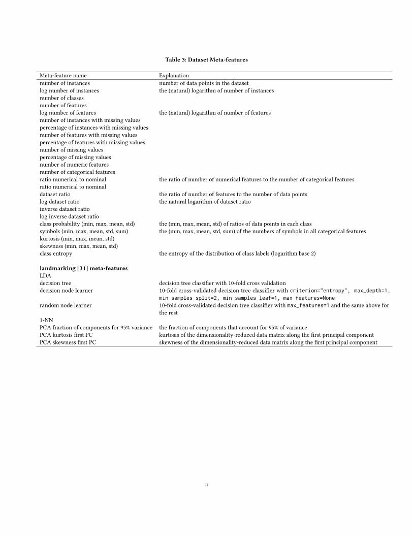
Table 3: Dataset Meta-features

Meta-feature name Explanationnumber of instances number of data points in the datasetlog number of instances the (natural) logarithm of number of instancesnumber of classesnumber of featureslog number of features the (natural) logarithm of number of featuresnumber of instances with missing valuespercentage of instances with missing valuesnumber of features with missing valuespercentage of features with missing valuesnumber of missing valuespercentage of missing valuesnumber of numeric featuresnumber of categorical featuresratio numerical to nominal the ratio of number of numerical features to the number of categorical featuresratio numerical to nominaldataset ratio the ratio of number of features to the number of data pointslog dataset ratio the natural logarithm of dataset ratioinverse dataset ratiolog inverse dataset ratioclass probability (min, max, mean, std) the (min, max, mean, std) of ratios of data points in each classsymbols (min, max, mean, std, sum) the (min, max, mean, std, sum) of the numbers of symbols in all categorical featureskurtosis (min, max, mean, std)skewness (min, max, mean, std)class entropy the entropy of the distribution of class labels (logarithm base 2)

landmarking [31] meta-features

LDAdecision tree decision tree classifier with 10-fold cross validationdecision node learner 10-fold cross-validated decision tree classifier with criterion="entropy", max_depth=1,

min_samples_split=2, min_samples_leaf=1, max_features=Nonerandom node learner 10-fold cross-validated decision tree classifier with max_features=1 and the same above for

the rest1-NNPCA fraction of components for 95% variance the fraction of components that account for 95% of variancePCA kurtosis first PC kurtosis of the dimensionality-reduced data matrix along the first principal componentPCA skewness first PC skewness of the dimensionality-reduced data matrix along the first principal component

11