object oriented hydrologic modeling with gis …vmerwade/reports/2011_02.pdf · object–oriented...

OBJECT–ORIENTED HYDROLOGIC MODELING WITH GIS

A Dissertation

Submitted to the Faculty

of

Purdue University

by

Kwangmin Kang

In Partial Fulfillment of the

Requirements for the Degree

of

Doctoral of Philosophy

May 2011

Purdue University

West Lafayette, Indiana

ii

To my wife, my daughter, my son, my parents and the rest of my family.

iii

ACKNOWLEDGMENTS

I would like to thank all of those who have encouraged, helped, and supported me

during my doctorate. First of all, I would like to thank my Ph.D. advisor, Professor

Venkatesh Merwade, for his support and encouragement over the past four years. I also

express my gratitude to my Ph.D. committee members, Professor Rao Govindaraju,

Professor Bernard Engel and Professor Dennis Lyn, for their guidance and

encouragement during Ph.D. research. Especially, I also appreciate Dr. Shivam Tripathi

for his continuous help. Finally, thanks are due to hydrology secretary, Mrs. Judith Haan,

and all my colleagues.

iv

TABLE OF CONTENTS

Page

LIST OF TABLES ............................................................................................................ vii

LIST OF FIGURES ........................................................................................................... ix

ABBREVIATIONS ........................................................................................................... xi

ABSTRACT ..................................................................................................................... xiii

CHAPTER 1. INTRODUCTION ....................................................................................... 1

1.1. Background .........................................................................................................1

1.2. Literature Review and Motivation ......................................................................2

1.2.1. Hydrologic Model .....................................................................................2

1.2.2. The problem of rainfall uncertainty for hydrologic model .......................4

1.2.3. The problem of DEM variations for hydrologic model ............................5

1.3. Objective of the study .........................................................................................7

CHAPTER 2. GIS AND HYDROLOGIC INFORMATION SYSTEM MODELING

OBJECT ...................................................................................................... 8

2.1. Introduction .........................................................................................................8

2.2. Object Orientation in Hydrology .......................................................................10

2.3. Hydrologic Modeling Objects ...........................................................................13

2.4. Updating the GHISMO Framework ..................................................................15

CHAPTER 3. DEVELOPMENT AND APPLICATION OF A

STORAGE–RELEASE BASED DISTRIBUTED HYDROLOGIC

MODEL USING GIS ................................................................................ 17

3.1. Introduction .......................................................................................................17

3.2. Background and Related Work .........................................................................19

v

Page

3.3. Study Area and Data .........................................................................................21

3.4. Model Development ..........................................................................................25

3.4.1. Conceptual Framework ...........................................................................25

3.5. Results ...............................................................................................................36

3.5.1. Model Calibration and Verification ........................................................36

3.5.2. Comparison with HEC–HMS .................................................................46

3.5.3. Comparison with time variant SDDH Model ..........................................49

3.6. Discussion .........................................................................................................52

3.7. Conclusions and Future Work ...........................................................................54

CHAPTER 4. IMPROVING RAINFALL ACCURACY ON DISTRIBUTED

HYDROLOGIC MODELING BY USING SPATIALLY UNIFORM

AND NON–UNIFORM NEXRAD BIAS CORRECTION ..................... 56

4.1. Introduction .......................................................................................................56

4.2. Study Areas and Data ........................................................................................59

4.3. NEXRAD Bias Correction Methods .................................................................63

4.3.1. Kalman filter ...........................................................................................63

4.3.2. Spatially uniform NEXRAD Bias Correction using Kalman filter .........66

4.3.3. Spatially non–uniform NEXRAD Bias Correction using

Kalman Filter .......................................................................................... 67

4.4. Results ...............................................................................................................69

4.4.1. Assessment of NEXRAD Rainfall Inputs ...............................................70

4.4.2. Sensitivity of Hydrographs to NEXRAD Bias Correction Schemes ......74

4.5. Summary and Conclusions ................................................................................89

CHAPTER 5. RESEARCH SYNTHESIS AND FURTURE WORK .............................. 92

5.1. Object–oriented hydrologic model ....................................................................92

5.2. Parameter Estimation for STORE DHM ...........................................................93

vi

Page

5.3. Critical Cell Travel Time Criteria .....................................................................93

5.4. Number of Rain gauge for correcting radar bias ...............................................94

LIST OF REFERENCES .................................................................................................. 95

APPENDICES

Appendix A. ...........................................................................................................106

Appendix B. ...........................................................................................................108

Appendix C. ...........................................................................................................110

VITA ............................................................................................................................... 112

vii

LIST OF TABLES

Table Page

3.1 Study sites details for the STORE DHM Application. .......................................... 22

3.2 Initial values of Manning‟s n. ................................................................................ 24

3.3 CCT for different grid resolutions using Cedar Creek DEM ................................. 35

3.4 Details of storm events for each site. ..................................................................... 37

3.5 Uncalibrated models results for Event 1 at each study site (C is

Cedar Creek, F is Fish Creek and R is Crooked Creek.). ....................................... 38

3.6 Manning‟s n for study areas. .................................................................................. 40

3.7 Calibration and validation results for all events (1–4) for Cedar

Creek (c), Fish Creek (F) and Crooked Creek (R) using gauge rainfall. .............. 41

3.8 Calibration and validation results for all events (1–4) for Cedar

Creek (c), Fish Creek (F) and Crooked Creek (R) using NEXRAD rainfall. ....... 42

3.9 HEC–HMS model results for Cedar Creek. ........................................................... 47

3.10 Time variant SDDH model results for Cedar Creek. ............................................. 50

4.1 Summary of storm events for application of NEXRAD bias correction. .............. 62

4.2 NEXRAD bias corrected rainfall statistics in the UWR basin. ............................. 72

4.3 NEXRAD bias corrected rainfall statistics in the UCR basin................................ 72

4.4 Calibrated Manning‟s n values for each event in the UWR basin. ........................ 74

4.5 Calibrated Manning‟s n values for each event in the UCR basin. ......................... 75

4.6 Calibrated simulation statistics for each event in the UWR basin. ........................ 77

4.7 Calibrated simulation statistics for each event in the UCR basin. ......................... 77

4.8 Details of simulation results with MPE NEXRAD bias corrected

rainfall input for the UWR basin. ........................................................................... 84

viii

Table Page

4.9 Details of simulation results with SNU–R NEXRAD bias corrected


4.10 Details of simulation results with SNU–E NEXRAD bias corrected


4.11 Details of simulation results with MPE NEXRAD bias corrected

rainfall input for the UCR basin. ............................................................................ 86

4.12 Details of simulation results with SNU–R NEXRAD bias corrected


4.13 Details of simulation results with SNU–E NEXRAD bias corrected


ix

LIST OF FIGURES

Figure Page

2.1 Object Model Diagram for GHISMO. ................................................................... 14

2.2 Update Object Model Diagram for GHISMO. ...................................................... 16

3.1 Example calculation in SDDH model. ................................................................... 20

3.2 Study Areas for the STORE DHM Application (C – Cedar Creek,

F – Fish Creek, R – Crooked Creek). ..................................................................... 23

3.3 Sample calculations using a 3 x 4 hypothetical grid. ............................................. 26

3.4 Storage release concept. ......................................................................................... 29

3.5 Cedar Creek model hydrographs with different DEM resolutions:

(a) STORE DHM simulation with 15min simulation time step:

(b) STORE DHM simulation using time step based on CCT. ............................... 34

3.6 Uncalibrated model results for Event 1 (C1, F1 and R1) using gauged

rainfall input. X–axis represents time in hours and Y–axis represents

flow in cubic meters per second. ............................................................................ 39

3.7 Cedar Creek model hydrographs. X–axis represents time in hours and Y–axis

represents flow in cubic meters per second. ........................................................... 43

3.8 Fish Creek model hydrographs. X–axis represents time in hours and Y–axis

represents flow in cubic meters per second. ........................................................... 44

3.9 Crooked Creek model hydrographs. X–axis represents time in hours and

Y–axis represents flow in cubic meters per second. .............................................. 45

3.10 Comparison of HEC–HMS and STORE DHM hydrographs with observed

data for Cedar Creek. X–axis represents time in hours and Y–axis represents


3.11 Comparison of time variant SDDH and STORE DHM hydrographs with

observed data for Cedar Creek. X–axis represents time in hours and

Y–axis represents flow in cubic meters per second. .............................................. 51

x

Figure Page

4.1 Study basin locations in relation to rain gauges and stream gauges

(UWR – Upper Wabash River basin, UCR – Upper Cumberland

River basin). ........................................................................................................... 60

4.2 Basin locations and surrounding NEXRAD StageIII. ........................................... 61

4.3 Scatter plot of NEXRAD bias corrected rainfall and cross–validated

observed gauge rainfall for (a) the UWR and (b) the UCR basins. ....................... 71

4.4 Time series of (a) Standard Deviation and (b) Variation. ...................................... 73

4.5 Calibrated model results for every event using NEXRAD rainfall

input (e.g. UWR1 represents event 1 for UWR basin). X–axis represents

time in hours and Y–axis represents flow in cubic meters per second. ................. 76

4.6 Storm Event 1 model hydrographs for both (a) the UWR basin and

(b) the UCR basin. X–axis represents time in hours and Y–axis represents














4.11 Storm events peak discharge (m3/s) scatter plots for (a) the UWR and

(b) the UCR basins. ................................................................................................ 88

xi

ABBREVIATIONS

HEC–HMS Hydrologic Engineering Center Hydrologic Modeling System

GIS Geographic Information System

DEM Digital Elevation Model

GHISMO GIS and Hydrologic Information System Modeling Objects

STORE DHM Store Released Based Distributed Hydrologic Model

SHE Système Hydrologique Europèen

IHDM Institute of Hydrology Distributed Model

CSIRO TOPOG Terrain Analysis Hydrologic Model

SDDH Spatially Distributed Direct Hydrograph Travel time method

RAS River Analysis System

SWAT Soil Water Assessment Tool

WMS Watershed Modeling System

Z–R Reflectivity – Rainfall

HDP Hourly Digital Precipitation

NEXRAD Next Generation Radar

CONUS Covering the entire Continental United States

RFC River Forecast Center

MPE Multisensor Precipitation Estimator

NWS National Weather Service

GOES Geostationary Operational Environmental Satellite

SCS Soil Conservation Service

CN Curve Number

xii

CCT Critical Cell Travel Time

AR1 Autoregressive Order One

MFB Mean Field Bias

IDW Inverse Distance Weight

HRAP Hydrologic Rainfall Analysis Project

NLCD National Land Cover Dataset

USGS United States Geological Survey

NRCS National Resources Conservation Service

OHRFC Ohio River Forecast Center

UWR Upper Wabash River Basin

UCR Upper Cumberland River Basin

ENS Nash Sutcliffe efficiency coefficient

R2 Co–efficient of determination

RMSE Root Mean Square Error

MAPE Mean Absolute Percentage Error

SNU–R Spatially non–uniform NEXRAD bias correction with rain gauge

interpolation

SNU–E Spatially non–uniform NEXRAD bias correction with radar bias

interpolation

xiii

ABSTRACT

Kang, Kwangmin. Ph.D., Purdue University, May 2011. Object–oriented Hydrologic

Modeling with GIS. Major Professor: Venkatesh Merwade.

A prototype geographic information system (GIS) based tightly coupled object

oriented framework called GIS and Hydrologic Information System Modeling Object

(GHISMO) is presented in this thesis. The proposed GHISMO framework is developed

within ArcGIS environment such that geographic datasets can be treated as hydrologic

objects that have properties and methods to simulate a hydrologic system. The overall

GHISMO framework consists of HydroShed as a super class which is composed of six

sub classes, namely, HydroGrid (for grid based data such as digital elevation model),

ParameterGrid (for grid based parameters such as land use type), HydroArea (for polygon

features such as lakes and reservoirs), HydroCatchment (for polygon features

representing catchments and watersheds), HydroLine (for polyline features such as

rivers) and HydroTable (for input and output tabular data). The GHISMO framework is

applied to develop a modular hydrologic modeling system called the Storage Release

based Distributed Hydrologic Model (STORE DHM). The storage–release concept uses

the travel time within each grid cell to compute how much water is stored or discharged

to the watershed outlet at each time step. The STORE DHM is tested by simulating

multiple hydrologic events in three watersheds in Indiana. In addition, the GHISMO

framework is tested for its flexibility to adopt additional modules by implementing three

rainfall bias correction methods to provide accurate input for the STORE DHM.

Application of STORE DHM to multiple hydrologic events in three different

watersheds in Indiana show that the model is able to predict runoff hydrographs for

different types of events in terms of storm duration, peak flow magnitude and time–to–

peak. In addition, STORE DHM output is compared with outputs from two hydrologic

xiv

models including Hydrologic Engineering Center‟s Hydrologic Modeling System (HEC–

HMS) and time variant Spatially Distributed Direct Hydrograph travel time method

(SDDH). Results from these comparisons show that the STORE DHM outperforms both

HEC–HMS and SDDH in terms of overall hydrograph shape and flow magnitude.

The flexibility of GHISMO framework is tested by extending it to include a rainfall

bias correction module. The rainfall bias correction module is then used to correct

NEXRAD radar rainfall by implanting two non–uniform bias correction techniques.

Results from STORE DHM simulations using the original NEXRAD rainfall and bias-

corrected rainfall created in this study shows that the model response is dictated by

rainfall variations in the study area. The performance of STORE DHM output is

relatively better in a larger watershed with high variable rainfall compared to a smaller

watershed with uniform rainfall pattern. The findings from this study are limited by the

number of watersheds used, and the quality of the data. More testing of the GHISMO

framework and its modules is needed to make the proposed framework applicable for

different watersheds with varying scales.

1

CHAPTER 1. INTRODUCTION

1.1. Background

The hydrologic system is dynamic; states of the system are frequently updated as

meteorological inputs and basin characteristics change. Modeling this dynamic behavior

imposes special requirements on data handling and process calculations that make

development of event–based hydrologic model a challenging task. In the past two

decades, many event–based hydrologic models have been developed such as HEC–HMS

(Hydrologic Engineering Center–Hydrologic Modeling System), VIC (Variable

Infiltration Capacity), DRAINMOD and VfloTM

(Vieux, Inc.). Nevertheless, most of the

existing models have limitations in representing hydrologic processes and therefore they

cannot guarantee realistic simulations. For example, HEC–HMS is a lumped model – it

does not account for spatial variations in hydrologic processes. Further, most of the

existing models are not standalone (they need external software to get data or to run

simulation, e.g. VfloTM

) which makes them unwieldy. In addition, these existing models

are also inflexible for investigating hydrological processes because it is difficult to add

new hydrological components in them. To overcome these limitations, this study

develops GIS and Hydrologic Information System Modeling Object (GHISMO), an

event–based distributed hydrologic model, in a single platform of ArcGIS software. The

GHISMO uses object–oriented programming approach which provides flexibility in

investigating new hydrologic processes without changing the basic model framework.

The objectives of this research are – (1) to make a prototype of an object–oriented

hydrologic model framework (called GHISMO); (2) to investigate the robustness of the

2

developed prototype framework through several case studies; and (3) to demonstrate the

flexibility of the modeling framework in overcoming critical modeling hurdles.

1.2. Literature Review and Motivation

1.2.1. Hydrologic Model

Watershed based hydrologic models are important tools in operational hydrology

and water resources planning and management. A watershed scale hydrologic model is a

simplified description of the hydrologic system of a watershed. Traditionally, statistical

and conceptual hydrologic models have treated input parameters as lumped over the

entire study watershed by ignoring the spatial variability of the physical system and its

processes. Specifically, these models cannot accurately represent and model the spatial

variation in meteorological and land surface conditions that affect various hydrologic

processes, and therefore cannot assure realistic simulations. With the availability of DEM

(Digital Elevation Model) and next generation radar (NEXRAD) rainfall data, grid based

hydrologic models are more effective in representing the variations of meteorological

forcing and land surface parameters. Also, geographic information system (GIS) allows

processing of grid and vector data, which has led to rapid progress in distributed

hydrologic modeling. However, an existing problem in hydrologic modeling is that the

available software for handling spatial information and for running model simulation is

not integrated in the same environment.

An object–oriented approach to hydrologic modeling increases model flexibility

and reduces efforts when adapting the model for new application, area and algorithm.

Rather than replacing an old code that already works, the model code can be extended

using the object–oriented characteristic of inheritance (Kiker et al., 2006). An object–

oriented approach allows for building an incremental model that can be adapted to

3

different watershed conditions (Wang et al., 2005). In spite of many advantages, the

object–oriented approach has found only limited applications in hydrologic modeling

(Band et al., 2000; Kralisch et al., 2005; Lal et al., 2005). Band et al. (2000) describes a

spatial object–oriented framework for modeling watershed systems to include

hydrological and ecosystem fluxes. Chen and Beschta (1999) developed a 3–dimensional

distributed hydrological model–OWLS (the Object Watershed Link Simulation model)

for dynamic hydrologic simulation and applied it to the Bear Brook watershed in Maine.

Garrote and Becchi (1997) employs object oriented programming techniques with

distributed hydrologic models for real–time flood forecasting. Boyer et al. (1996)

presents an object–oriented method to simulate a rainfall–discharge relationship using a

lumped hydrologic model. McKim et al. (1993) introduced an object–oriented approach

to simulate hydrologic processes, specifically infiltration excess overland flow. The

above applications used object–oriented approach and achieved reasonable results for

hydrologic simulations. However, object–oriented approach is not comprehensively

discussed in the hydrologic literature and no general guideline exists for implementing

them in hydrologic models (Wang et al., 2005 and Kiker et al., 2006).

With the advent of remote sensing technology in topography analysis, several

distributed grid–based hydrologic models have been developed. These include SHE

(Système Hydrologique Europèen, Abbott et al., 1986), IHDM model (Institute of

Hydrology Distributed Model, Calver and Wood, 1995), the CSIRO TOPOG model

(Terrain Analysis Hydrologic Model, Vertessy et al., 1993) and HILLFLOW (Bronstert

and Plate, 1997). These models use grid–based routing (kinematic wave or diffusive

wave) approach to account for spatio–temporal variations in water movement. However,

they use complex algorithms with low computational efficiency requiring a large data

base for calibration and large computational resources for simulation (Beven, 2001).

Recently, several event–based grid models have been developed that use travel time

method for routing the flow through a watershed. These include: (i) the spatially

distributed unit hydrograph method by Maidment et al., (1993, 1996; Muzik 1995;

Ajward, 1996), (ii) the first passage–time response function which is derived from the

advection–dispersion method by Olivera and Maidment (1999), (iii) diffusive transport

4

method by Liu et al. (2003), and (iv) spatially distributed travel time method by Melesse

and Graham (2004), among others. Maidment (1993) assumed a time–invariant velocity

to get the unit hydrograph; whereas Muzik (1995) and Ajward (1996) used continuity and

Manning‟s equations to determine the flow velocity through each cell. Melesse and

Graham (2004) propose an integrated technique using remote sensing and GIS datasets to

compute spatially distributed excess rainfall, which was then routed by using the travel

time concept without relying on the unit hydrograph theory. Although these techniques

provided satisfactory results, the flow from each grid cell is routed through the system

independently without considering the interaction of neighboring cells as the water flows

downstream.

1.2.2. The problem of rainfall uncertainty for hydrologic model

Rainfall is a critical factor in hydrologic simulation. However, rainfall varies

substantially in space and time and therefore it is often poorly represented in hydrologic

models. Numerous studies in the past decades have investigated the sensitivity of runoff

hydrographs to spatial and temporal variations in precipitation. Faures et al. (1995)

concluded that for realistic hydrologic simulations, even for small watersheds, hydrologic

models require detailed information of the spatial rainfall patterns. This result agreed

with Wilson et al. (1979), who showed that the spatial distribution of rainfall had a

marked influence on the runoff hydrograph from a small catchment. Troutman et al.

(1989) investigated the effect of rainfall variability on model simulation, and concluded

that improper representation of rainfall variability over a basin would lead to

overestimation or underestimation of runoff.

Combining radar and gauge information produces improved precipitation estimates,

in terms of both quality and spatial resolution, in comparison with either radar or gauge

estimates alone (Smith and Krajewski, 1991). However, uncertainty persists in MPE

(Multisensor Precipitation Estimator) products because large portions of the radar

5

coverage area do not have rain gauge data to adjust biases in radar rainfall (Ciach and

Krajewski, 1999). Habib et al. (2009) studied a small watershed with dense rain gauge

network in south Louisiana and found that the MPE products tend to overestimate small

rain rates and underestimate large rain rates. They suggested that dense rain gauge

observations can improve MPE performance; however, maintaining a dense rain gauge

network in a large catchment is costly and impractical.

Winchell et al. (1998) investigated the effects of uncertainty in NEXRAD

estimated precipitation input on simulation of runoff. Specifically, they studied the

sensitivity of surface runoff to uncertainty in precipitation estimates arising from the

transformation of radar reflectivity to precipitation rate and from spatio–temporal

aggregation of the precipitation field. They found that the infiltration–excess mode of

surface runoff generation is more sensitive to precipitation uncertainties than the

saturation–excess mode of surface runoff generation. The study concluded that a limited

number of rain gauges may not completely eradicate biases in the radar data and may

lead to poor runoff simulations. In recent years, the availability of high–resolution

precipitation data from different weather radar platforms has intensified the research on

understanding the effects of spatial resolution in precipitation data on hydrologic

simulations.

1.2.3. The problem of DEM variations for hydrologic model

Topographically–based modeling of catchment processes is becoming popular in

applied environmental research, mainly due to the advances in availability and quality of

DEM (Moore et al., 1991; Goodchild et al., 1993; Wise, 2000). Presently, DEM is used in

terrain modeling applications such as distributed hydrologic models (Beven and Moore,

1993), prediction of surface saturation zones (O‟Loughlin, 1986), erosion deposition

models (Desmet and Govers, 1996; Schoorl et al., 2000), and hillslope stability and

landslide hazard models (Montgomery and Dietrich, 1994; Tarboton, 1997). Analysis in

6

DEM include automatic delineation of catchment areas (O‟Callaghan and Mark, 1984;

Martz and De Jong, 1998), development of drainage networks (Fairfield and Leymarie,

1991), detection of channel heads (Montgomery and Dietrich, 1994), determination of

flow accumulation (Peuker and Douglas, 1975), and flow direction and routing (Tarboton,

1997). Wilson et al. (2000) demonstrated that (a) slope gradient and specific area of the

catchment tend to decrease as DEM cell size increases, (b) larger DEM cell sizes produce

shorter total flow length in a watershed, and (c) the accuracy of slope gradient decreases

with increase in DEM cell size. The DEM resolution is expected to affect the delineation

of watersheds which in turn would influence hydrologic model performance (Madsen,

2003). However, the effect of DEM resolution on the performance of a hydrologic model

is not yet well understood (Vazquez et al., 2004).

Zhang and Montgomery (1994) used DEM of different resolutions in conjunction

with eight flow–direction algorithms to detect patterns in storm runoff and surface

saturation. They found that DEM sizes significantly affect computed topographic

parameters and hydrographs in TOPMODEL simulation. Studying a watershed in Iowa

using KINEROS (kinematic runoff and erosion model) Kalin et al. (2003) observed that

increasing the DEM resolution increases the magnitude of peak flow without affecting its

time of occurrence. FitzHugh and Mackay (2000) investigated a watershed in Wisconsin

using SWAT (Soil and Water Assessment Tool) and observed that sediment yield from a

watershed delineated using a fine resolution DEM (10m) dropped by 44% in comparison

to a watershed delineated using a coarse resolution DEM (500m). All the aforementioned

studies on DEM found that the DEM resolution significantly affects the computation of

slope, catchment area, flow direction and surface runoff. Thus hydrologic model

simulations are very sensitive to DEM resolution.

7

1.3. Objective of the study

The overall goal of this research effort is to develop an efficient and robust event–

based distributed hydrologic model under ArcGIS environment that can overcome some

of the existing hurdles of hydrologic modeling through an object–oriented approach. To

accomplish this objective, the following tasks were executed:

(1) Develop a prototype of GIS based object–oriented framework for hydrologic

modeling.

(2) Test robustness of the developed prototype by applying it to various storm events

over different study areas.

(3) Demonstrate the flexibility of developed prototype in linking additional

objects/modules to it.

The remainder of this dissertation is structured as follows. In Chapter 2, description

of the GHISMO diagram is introduced. In Chapter 3, development and application of

grid–based distributed hydrologic model is presented. Chapter 4 presents the

implementation module for correcting spatially distributed rainfall bias.

8

CHAPTER 2. GIS AND HYDROLOGIC INFORMATION SYSTEM MODELING

OBJECT

2.1. Introduction

Computer based models have been used as planning tools in water resources

management over the last three decades. The researches in computational water resources

are well known and organized. Also, many models are applied to resolve a variety of

hydrologic components (Abbott et al., 1993). It is necessary to combine several of these

models (e.g., surface water model, groundwater model and reservoir model) to bring a

holistic idea in water resources planning and management. Realization of this approach

requires a modular structure in water resources research, and it allows different sub–

models to be interconnected depending on the hydrologic system. Another important

aspect that must be considered in new development of hydrologic models is creating

software elements that can be adapted in future projects. If a modular structure provides

reusable components, both regarding development time and reliability of the software

produced, it will be an extensive water resources platform (Goldberg et al., 1995). This

also will reduce development and maintenance cost for the project.

Running a hydrologic model involves several steps including data collection, pre–

processing, parameter estimation, calibration and validation. With the advancement in

data collection methods and their representation in digital form, the use of GIS is

common for data management, pre–processing and post–analysis in any hydrologic

modeling study (Maidment, 1993). While GIS provides a user friendly visual

environment for handling hydrologic data, it lacks the computational engine to perform

hydrologic simulations. Also, many hydrologic models have limitations of GIS

9

capabilities for data handling, pre–processing and visualization. As a result, several

efforts have been made to couple GIS with hydrologic models. These efforts include: (i)

the development of GIS tools for Hydrologic Engineering Center‟s (HEC) Hydrologic

modeling system (HMS) and River Analysis System (RAS) models [U.S. Army Corps of

Engineers (USACE)]; (ii) the integration of GIS and modeling tools in EPA BASINS

analysis environment (Lahlou et al., 1998); (iv) the development of a GIS pre–processor

for the Soil Water Assessment Tool (SWAT; Luzio et al., 2002); and (v) the development

of Watershed Modeling System (WMS; Environmental Modeling Research Laboratory,

Nelson 1997).

Most previous attempts listed above to link GIS and hydrologic models can be

categorized as „loosely coupled‟ because both systems act independent of each other, and

are only linked through input or output data. For example, GIS tools are used to develop

the input file, which is then used to run the hydrologic model. Any changes in the model

domain or input attributes during the modeling process are not reflected in the data that

are used in creating the model input. With the availability of high resolution geospatial

and temporal data, and improved capability of GIS to handle continuous, dynamic

datasets including time series, it is now possible to expand the role of GIS beyond that of

a pre– or post–processing tool for hydrology to a tightly coupled modeling environment

where GIS can perform hydrologic simulations.

If a hydrologic model investigates a new hydrologic component within the frame,

an object–oriented approach allows for increased model flexibility without changing the

main frame. The model codes that already exist in the old module can be extended by

using the inheritance characteristic through an object–oriented approach (Kiker et al.,

2006). In recent years, object–oriented based hydrologic models are increasingly used in

water resources research, and also the modeling paradigm in water resources is changing

to the object–oriented approach (Wang et al., 2005). Creating an incremental watershed

model can be made by object–oriented design methods and using an object–oriented

programming language (Wang et al., 2005), and this model can be applied to various

watershed conditions. Even though object–oriented based hydrologic models have

attractive advantages, few object–oriented based hydrologic models exist, and there is no

10

detailed discussion for the principle of object–oriented hydrologic approach (e.g. Band et

al., 2000; Kralisch et al., 2005; Lal et al., 2005).

The most advanced water resources modeling research is increasing model

flexibility to consider comprehensive natural phenomena. In addition, constructing this

model can promote an extension of new hydrologic components by reducing inefficient

efforts. This research presents the development of a new prototype hydrologic model

frame, GIS and Hydrologic Information System Modeling Object (GHISMO), developed

with an object–oriented approach. It should be noted that the objective of this work is not

to create another model, but to create a framework where different models or their

components can interact with each other within a GIS environment to overcome

hydrologic modeling issues through an object–oriented approach.

2.2. Object Orientation in Hydrology

According to Bian (2007), object orientation involves three levels of abstractions:

object oriented analysis, object oriented design, and object oriented programming. Object

oriented analysis involves conceptual representation of the world including the facts and

relationships about a situation. In hydrology, this would mean the conceptual

representation of a watershed as a set of objects to include streams and corresponding

catchments. Object oriented design uses the conceptual representation from object

oriented analysis to create a formal model of objects, their properties, events, and

relationships. Object oriented programming involves the implementation of objects and

their events to accomplish a certain task. Object orientation relies on two basic principles:

encapsulation and composition. Encapsulation considers that the world is composed of

objects, and that each object has an identity, properties and behavior. The properties of an

object are defined by its attributes (e.g., length, area), and the behavior is represented by

methods. While the value of an attribute can define the state of an object, a method can

change the state of an object, and that change is referred to as an event. For example, a

11

river object will have properties such as length and slope, methods such as RouteFlow

and ComputeStorage, and routing a hydrograph through the river (by using RouteFlow

method) is an event.

The principle of composition describes how objects are related through

relationships including inheritance, aggregation and association. In object orientation, all

objects belong to object classes, and all classes are hierarchal. A sub-class is a kind of

this own super-class (through inheritance) and inherits all properties and methods from

the super class, but also may have its own additional properties and methods. An object

can also be a part of another object (through aggregation), and can simultaneously

maintain relationships with other objects (through association). For example, an

AlluvialRiver class can be a sub–class of River super class (inheritance), a River class

can be a part of RiverNetwork class (aggregation) and River class is related with

Watershed class through streamflow (relationship). Past studies that used object

orientation for hydrologic modeling include Whittaker et al. (1991) who used object–

oriented approach to model infiltration excess overland flow. Boyer et al. (1996) used

object oriented approach to develop a lumped rainfall–runoff model. McKim et al. (1993)

used object orientation to combine remote sensing and hydrologic data to develop a

forecast model. Garrote and Becchi (1997), Band et al. (2000), and Wang et al (2005)

proposed object oriented frameworks for modeling hydrologic processes at watershed

scale. Most of these studies used object orientation to model hydrologic processes using

the concepts of inheritance and aggregation. Recently, Richardson et al. (2007) proposed

a prototype geographically based object framework for linking hydrologic and

biochemical processes in the sub–surface. The process objects, however, were loosely

coupled with geographic objects, thus leaving an opportunity for a tightly coupled

geographically based object oriented modeling.

Relatively recent advances in GIS have enabled adaption of object orientation in

storing and handling geospatial and temporal hydrologic data in research and practice.

For example, Arc Hydro (Maidment, 2002) uses an object oriented approach to represent

hydrologic environment through feature, object and relationship classes within a

geodatabase. In Arc Hydro, a HydroEdge (stream) is sub class of generic Polyline super

12

class (inheritance), and is a part of HydroNetwork (aggregation). HydroEdge is related to

Watershed (which itself is a sub–class of Polygon super class) through a common

identifier (HydroID). Thus, ArcHydro uses object orientation to develop a physical

representation of hydrography by using GIS objects. Thus, by knowing the HydroID of

any geographic feature, it is possible to trace the flow of water by using points, lines, and

polygons at multiple scales including at continental scale. The National Hydrography

Dataset (NHD) available for the entire United States from the United States Geological

Survey (USGS) also uses the object oriented (or geodatabase) design to provide data to

its users.

The geodatabase approach to hydrology data overcomes several practical issues

which are associated with storing and handling heterogeneous multi–scale data by

providing a relational data model. Besides overcoming the data issues, the geodatabase

approach provides an opportunity to exploit the potential of object oriented approach to

overcome the limitations of scale and parameterization in distributed modeling of

hydrologic processes. For example, if a polygon representing a watershed in GIS is

treated as a hydrologic object that has some properties (e.g. area and slope) and methods

(to compute runoff and route flow), then multiple watersheds can be linked and executed

in parallel to scale–up the modeling domain from one single watershed to larger (national

or continental) scales. Similarly, the availability of increasing GIS layers to represent soil,

landuse and topography at multiple scales, can enable parameterization of hydrologic

processes (or watershed methods) through GIS tools, which is not possible with most

existing models that do not explicitly work within a GIS environment. This research

builds on past studies to create a prototype tightly coupled object oriented GIS based

hydrologic model to simulate hydrologic processes using geospatial inputs. The prototype

modeling approach presented in this research is developed by using Visual Basic and

ArcObjects within ArcGIS, and is referred to as GIS and Hydrologic Information System

Modeling Objects (GHISMO).

13

2.3. Hydrologic Modeling Objects

An object–oriented hydrologic model framework is implemented in ArcGIS by

developing hydrologic modeling objects as shown in Fig. 2.1. The hydrologic modeling

object framework implements both principles of aggregation (represented with diamond)

and inheritance (represented with triangle arrow) as shown in Fig. 2.1. HydroShed is the

highest level class that includes the following six classes: (1) HydroGrid (to process

gridded hydrologic information such as topography and rainfall), (2) ParameterGrid (to

process gridded hydrologic parameters such as Mannings n), (3) HydroArea (to process

vector hydrologic data for lakes and rivers), (4) HydroCatchment (to process vector

hydrologic data for catchments or sub–watersheds), (5) HydroLine (to process vector

hydrologic data for streams), and (6) HydroTable (to process tabular data). As displayed

in Fig. 2.1, those classes dealing with raster, vector and tables are implemented in this

research.

ProcessGrid (to implement hydrologic processes) and TopoGrid (to implement

terrain processes) are two sub–classes of the HydroGrid class. ProcessGrid can work on

gridded data to implement hydrologic processes to create excess rainfall and runoff

hydrograph by implementing specific sub–classes such as ExRain and Hydrograph as

shown in Fig. 2.1. ExRain implements specific techniques such as SCS curve number

(through SCS sub–class) and Green–Ampt (through GreenAmpt sub–class) to compute

excess rainfall using the rainfall input. Hydrograph class implements specific techniques

such as storage release to compute runoff hydrograph from excess rainfall. TopoGrid

implements sub–classes to create terrain attributes such as flow direction, flow

accumulation, stream network and catchment by using topography data (DEM).

HydroArea can work on flow transformation by implementing specific techniques

such as SCS dimensionless unit hydrograph (through SCSUnit sub–class) and Clark unit

hydrograph (through ClarkUnit sub–class) for vector data. Also, HydroLine can work on

river routing by implementing specific techniques such as Kinematic wave river routing

(through KinematicWave sub–class) and Muskingum river routing (through Muskingum

sub–class).

14

+Method()

-Attribute

HydroArea

+Method()

-Attribute

HydroShed

+Method()

-Attribute

HydroCatchment

+Method()

-Attribute

TopoGrid

+Method()

-Attribute

ParameterGrid+Method()

-Attribute

ProcessGrid

+Method()

-Attribute

HydroGrid

+Method()

-Attribute

ExRain

+Method()

-Attribute

SCS

+Method()

-Attribute

Hydrograph

+Method()

-Attribute

GreenAmpt

+Method()

-Attribute

HydroLine

+Method()

-Attribute

HydroTable

+Method()

-Attribute

TSTable

+Method()

-Attribute

ParameterTable

+Method()

-Attribute

PairTable

1*

1 *

1* 1

*

1

*

1

*

+Method()

-Attribute

ClarkUnit

+Method()

-Attribute

SCSUnit

+Method()

-Attribute

Muskingum

+Method()

-Attribute

KinematicWave

Figure 2.1 Object Model Diagram for GHISMO.

15

HydroTable implements three tables: TSTable, ParameterTable and PairTable.

TSTable class processes time series table (e.g., rainfall and streamflow time series);

ParameterTable processes parameter values linked to geographic features (e.g.,

Manning‟s n values for different land cover types); and PairTable processes paired data

such as stage–discharge rating curves.

2.4. Updating the GHISMO Framework

An object in GHISMO allows creating a class or a function to handle a variety of

hydrologic components. The GHISMO provides flexibility in modular development of

the model without changing the basic framework through object–oriented approach, if

hydrologic mechanisms need more advanced investigations. For example, this research

creates a new object, RadarBias (to implement three different radar bias correction

processes), to investigate the effect of different radar bias corrected rainfall inputs on

hydrologic simulations as shown in Fig. 2.2. The GHISMO allows adding a RadarBias

object that is a part of the new modeling processes without changing its main framework

because the GHISMO is designed to be open to extension. The greatest benefit in the

application of this design approach (open for extension for modification) is reusability

and maintainability, and its advantages can overcome a prospective hydrologic modeling

issue, such as making a large and complex hydrologic model. Specific methodology and

application of hydrologic modeling as a part of the GHISMO framework are described in

Chapter 3, and methodology and application of updating RadarBias object are also

described in Chapter 4.

16

+Method()

-Attribute

HydroArea

+Method()

-Attribute

HydroShed

+Method()

-Attribute

HydroCatchment

+Method()

-Attribute

TopoGrid

+Method()

-Attribute

ParameterGrid+Method()

-Attribute

ProcessGrid

+Method()

-Attribute

HydroGrid

+Method()

-Attribute

ExRain

+Method()

-Attribute

SCS

+Method()

-Attribute

Hydrograph

+Method()

-Attribute

GreenAmpt

+Method()

-Attribute

HydroLine

+Method()

-Attribute

HydroTable

+Method()

-Attribute

TSTable

+Method()

-Attribute

ParameterTable

+Method()

-Attribute

PairTable

1*

1 *

1* 1

*

1

*

1

*

+Method()

-Attribute

RadarBias

+Method()

-Attribute

ClarkUnit

+Method()

-Attribute

SCSUnit

+Method()

-Attribute

Muskingum

+Method()

-Attribute

KinematicWave

Figure 2.2 Update Object Model Diagram for GHISMO.

17

CHAPTER 3. DEVELOPMENT AND APPLICATION OF A STORAGE–RELEASE

BASED DISTRIBUTED HYDROLOGIC MODEL USING GIS

3.1. Introduction

Hydrologic model development is complicated by the nonlinear, time dependent

and spatially varying nature of rainfall–runoff mechanism (Remesan, 2009). The rainfall–

runoff process is affected by many factors such as rainfall dynamics, topography, soil

type and land use. Significant advancements in hydrological modeling started with the

introduction of unit hydrograph model and its related impulse response function

(Sherman, 1932). Since then, a myriad of hydrologic models have been developed,

calibrated and validated for several watersheds at different scales. Developing a realistic

hydrologic model requires an understanding of the interrelation between parameterization

and scale because as the scale of the hydrologic modeling problem increases, the

complexity of the model increases as well (Famiglietti, 1994).

The commonly used HEC–HMS (Hydrologic Engineering Center Hydrologic

Modeling System; USACE, 1998) model does not account for spatial variations in

hydrologic processes because it is a lumped hydrologic model which treats input

parameters as an average over the watershed. In addition, use of HEC–HMS requires

external software such as HEC–GeoHMS to produce necessary input files for the model.

HEC–GeoHMS is an ArcGIS toolbar to process digital information related to topography,

land use, and soil to produce input files for HEC–HMS. Because of their simplicity in

terms of data requirements, model parameterizations and application, lumped hydrologic

models such as HEC–HMS have been very popular in hydrology.

18

Application of semi–distributed or distributed models is complicated due to data

requirements for physically based models (Koren et al., 2003), and parameter estimation

for conceptual models (Moreda et al., 2006). To fully exploit the strength of semi–

distributed and distributed models, it is necessary to provide data that can capture the

spatio–temporal variations in the hydrologic system including rainfall dynamics.

Difficulties related to data requirements for spatially distributed hydrologic models are

addressed by the availability of continuous digital data in the form of digital elevation

model (DEM) and gridded radar rainfall. In addition to the availability of geospatial data,

the use of geographic information system (GIS) to process grid and vector data has led to

rapid progress in grid based distributed hydrologic modeling (e.g., Maidment, 1993;

Olivera and Maidment, 1999; Melesse et al., 2004). The use of spatially distributed

topographic, soils, land use, land cover, and precipitation data in GIS ready format

provides the framework for the development, verification, and eventual acceptance of

new hydrologic models capable of taking full advantage of these new data, while

acknowledging the uncertainty inherent in the data.

The broader goal of this study is to create a conceptual hydrologic model

framework, called GIS and Hydrologic Information System Modeling Objects

(GHISMO), which can utilize GIS data at different resolutions, and use these data to

simulate hydrologic processes at multiple scales. GHISMO is expected to provide a

platform where different models or their components can interact with each other within

a GIS environment to overcome the issues related to computational requirements, scale

and versatility through an object oriented design. As a first step towards accomplishing

this broader goal, this chapter presents the development and application of a prototype

grid based hydrologic model using object oriented programming concepts. The data and

computational side of GHISMO is developed by using ArcObjects (building blocks or

objects of the ArcGIS software), and the conceptual model for hydrologic simulations is

based on a simple storage–release approach. In the storage–release approach, each cell in

a raster grid provides storage for the water draining to it from neighboring cells, and then

the water is released to downstream cells based on the travel time computed by

combining the continuity and Manning‟s equations. This chapter specifically presents the

19

conceptual framework of the prototype hydrologic model, and its application to three

study sites in Indiana. The grid based hydrologic model will be referred as the Storage

Released based Distributed Hydrologic Model (STORE DHM).

3.2. Background and Related Work

Maidment (1993) proposed a time–area method within raster GIS to derive a

spatially distributed unit hydrograph. Maidment‟s method uses a DEM to determine the

flow direction from each cell based on the maximum downhill slope, and flow velocity

through each cell is estimated based on the kinematic wave assumption. The travel time

through each cell is then obtained by dividing the flow distance by the flow velocity.

Maidment demonstrated that if a constant velocity can be estimated for each grid cell, a

flow time grid can be obtained and subsequently isochronal curves and a time–area

diagram can be determined for a watershed. Maidment‟s method is based on velocity

time invariance in a linear hydrologic system.

Melesse and Graham (2004) proposed a grid based cell travel time hydrologic

model that assumes invariant travel times during a storm event. The runoff hydrograph at

the outlet of watershed is developed by routing the spatially distributed excess

precipitation through the watershed using topographic data. Calculation of travel times

from each cell to the watershed outlet requires computation of a runoff velocity for each

grid cell. Velocity for each grid cell can be estimated depending on whether the grid cell

represents an area of diffuse overland flow or more concentrated channel flow. This

method ignores the variations in travel time during the storm because it takes average

excess rainfall intensity. The advantage of Melesse and Graham‟s grid–based travel time

method is that it can create a direct hydrograph without a spatially lumped unit

hydrograph during a rainfall event.

The issue of invariant travel time proposed by Melesse and Graham (2004) is

addressed by Du et al. (2009), who proposed a time variant spatially distributed direct

20

hydrograph travel time method (SDDH) to route spatially and temporally distributed

surface runoff to the watershed outlet. In the time variant SDDH method, the cumulative

direct runoff and travel time are calculated by summing the individual volumetric flow

rates and travel times from all contributing cells to outlet along a flow path for a given

time step. This approach, however, cannot maintain the total mass balance because a cell

that receives input from multiple upstream cells gets accounted multiple times while

computing the flow from upstream cells. Similarly a particular cell does not account for

flow from adjacent cells while the flow is being routed from an upstream cell. For

example, in Fig. 3.1, water from cell A flows to the outlet cell H through cells D–E–H.

Similarly, water from cell B reaches the outlet through D–E–H. So if the flow at the

outlet from cells A and B is computed as cumulative flow along the flow path, flows

from D, E and H are accounted twice, thus compromising the mass balance. As a result,

this technique requires adjustment of travel time (which is mistakenly referred to as

calibration) to account for high volumetric flow rates computed through repeated

accumulations. To overcome these issues in grid based hydrologic models based on

travel–time concept, this study proposes a simple conceptual approach for distributed

event based hydrologic modeling using the storage release approach.

A B C

D E F

G H I

(a) Cell Identifier (b) Flow Direction

Figure 3.1 Example calculation in SDDH model.

21

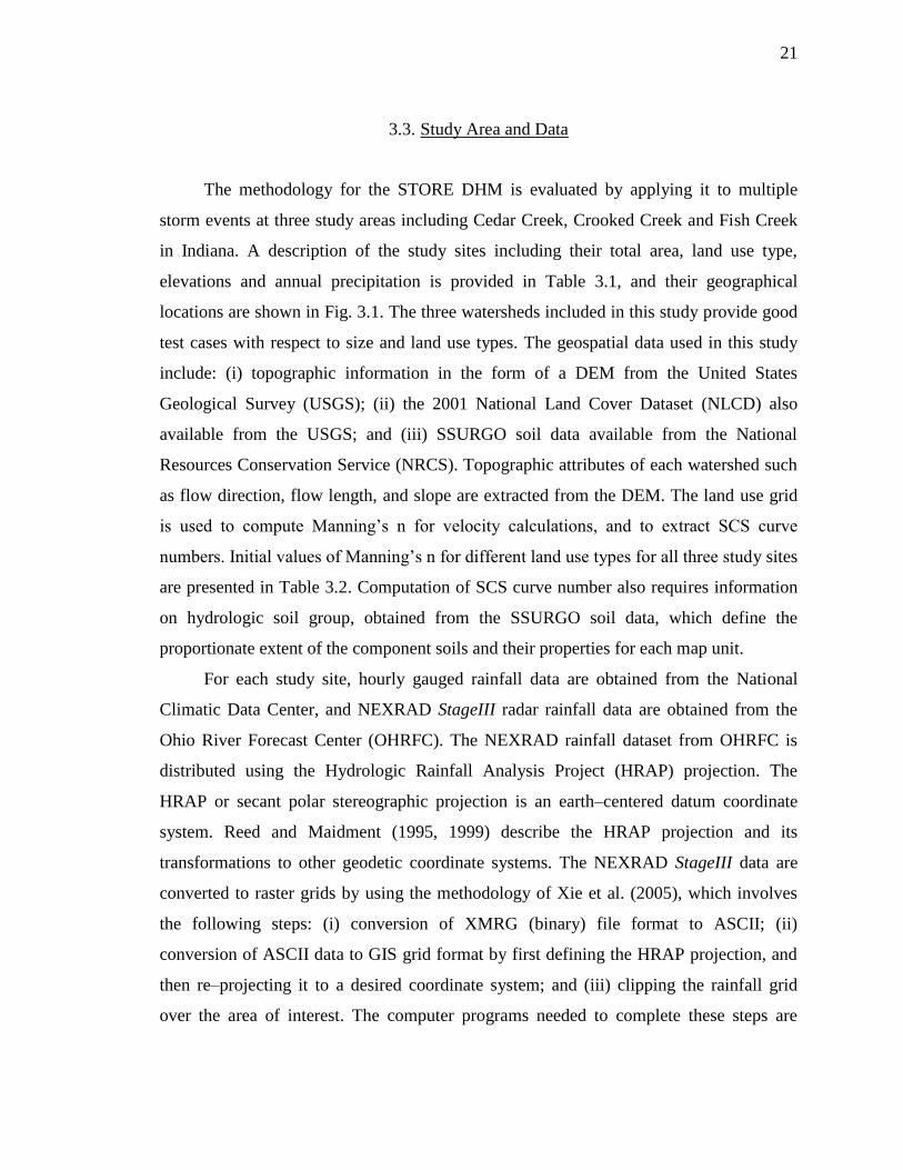
3.3. Study Area and Data

The methodology for the STORE DHM is evaluated by applying it to multiple

storm events at three study areas including Cedar Creek, Crooked Creek and Fish Creek

in Indiana. A description of the study sites including their total area, land use type,

elevations and annual precipitation is provided in Table 3.1, and their geographical

locations are shown in Fig. 3.1. The three watersheds included in this study provide good

test cases with respect to size and land use types. The geospatial data used in this study

include: (i) topographic information in the form of a DEM from the United States

Geological Survey (USGS); (ii) the 2001 National Land Cover Dataset (NLCD) also

available from the USGS; and (iii) SSURGO soil data available from the National

Resources Conservation Service (NRCS). Topographic attributes of each watershed such

as flow direction, flow length, and slope are extracted from the DEM. The land use grid

is used to compute Manning‟s n for velocity calculations, and to extract SCS curve

numbers. Initial values of Manning‟s n for different land use types for all three study sites

are presented in Table 3.2. Computation of SCS curve number also requires information

on hydrologic soil group, obtained from the SSURGO soil data, which define the

proportionate extent of the component soils and their properties for each map unit.

For each study site, hourly gauged rainfall data are obtained from the National

Climatic Data Center, and NEXRAD StageIII radar rainfall data are obtained from the

Ohio River Forecast Center (OHRFC). The NEXRAD rainfall dataset from OHRFC is

distributed using the Hydrologic Rainfall Analysis Project (HRAP) projection. The

HRAP or secant polar stereographic projection is an earth–centered datum coordinate

system. Reed and Maidment (1995, 1999) describe the HRAP projection and its

transformations to other geodetic coordinate systems. The NEXRAD StageIII data are

converted to raster grids by using the methodology of Xie et al. (2005), which involves

the following steps: (i) conversion of XMRG (binary) file format to ASCII; (ii)

conversion of ASCII data to GIS grid format by first defining the HRAP projection, and

then re–projecting it to a desired coordinate system; and (iii) clipping the rainfall grid

over the area of interest. The computer programs needed to complete these steps are

22

available from the National Weather Service‟s office of hydrology web site

(HTTP://WWW.NWS.NOAA.GOV/OH/HRL/DMIP/ NEXRAD.HTML).

The streamflow data for the study sites are obtained from the USGS Instantaneous

Data Archive web site (HTTP://IDA.WATER.USGS.GOV/IDA/). The streamflow values

from USGS include both base flow and surface runoff. In this study, the straight line base

flow separation method is used for retrieving surface runoff hydrographs from

streamflow.

Table 3.1 Study sites details for the STORE DHM Application.

Watershed Area

(km2)

Land use

Elevation

Range

(m)

Average

Slope

(%)

Annual

Precipitation

(mm)

Cedar

Creek 707

Agricultural

(76%); forest

(21%); urban

(3%)

238 –

324 3 1100

Fish

Creek 96

Agricultural

(82%); urban

(9%)

268 –

324 3.2 900

Crooked

Creek 46

Urban (88%);

agricultural (6%);

forest (6%)

217 –

277 1.2 880

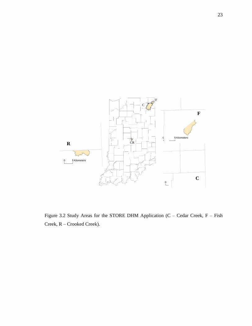
http://www.nws.noaa.gov/oh/hrl/dmip/%20nexrad.html

http://ida.water.usgs.gov/ida/

23

Figure 3.2 Study Areas for the STORE DHM Application (C – Cedar Creek, F – Fish

Creek, R – Crooked Creek).

0 5 Kilometers

0 5 Kilometers

0 5 Kilometers

C

F

CR

F

C

R

24

Table 3.2 Initial values of Manning‟s n.

Land use Range Initial Value

Agricultural 0.030–0.500 0.220

Forest 0.035–0.160 0.110

Developed 0.011–0.035 0.035

Water 0.025–0.033 0.033

25

3.4. Model Development

As mentioned in the Introduction section, the hydrologic model proposed here is a

part of a broader modeling framework using object oriented concepts in GIS. In a

nutshell, this object oriented framework uses a DEM as a hydrologic object that has

properties and methods such as ComuteRunoff and RouteFlow to perform hydrologic

simulations. The algorithm presented in this paper includes one set of methods that this

grid based hydrologic object can implement. The object can be extended to implement

additional methods including the ones from existing grid based models. The details of

this object oriented framework are beyond the scope of Chapter 3, and only the

conceptual framework behind the hydrologic modeling algorithm (STORE DHM) is

presented.

3.4.1. Conceptual Framework

The conceptual framework for the STORE DHM involves computing excess

rainfall, volumetric flow rate, and travel time to the basin outlet by combining steady

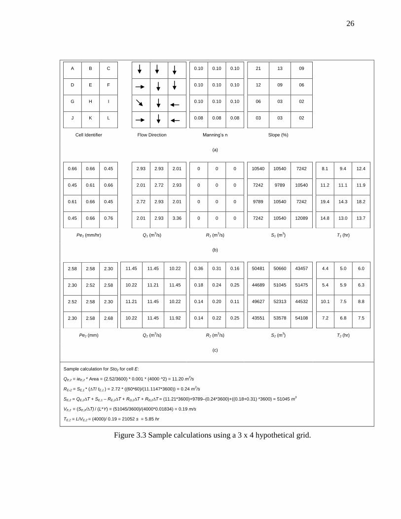
state uniform flow approximation with Manning‟s equation. Basic elements of this

conceptual framework are presented below followed by an example demonstration using

Fig. 3.3.

26

A B C

D E F

G H I

J K L

0.10 0.10 0.10

0.10 0.10 0.10

0.10 0.10 0.10

0.08 0.08 0.08

21 13 09

12 09 06

06 03 02

03 03 02

Cell Identifier Flow Direction Manning’s n Slope (%)

(a)

0.66 0.66 0.45

0.45 0.61 0.66

0.61 0.66 0.45

0.45 0.66 0.76

2.93 2.93 2.01

2.01 2.72 2.93

2.72 2.93 2.01

2.01 2.93 3.36

0 0 0

0 0 0

0 0 0

0 0 0

10540 10540 7242

7242 9789 10540

9789 10540 7242

7242 10540 12089

8.1 9.4 12.4

11.2 11.1 11.9

19.4 14.3 18.2

14.8 13.0 13.7

Pe1 (mm/hr) Q1 (m3/s) R1 (m

3/s) S1 (m

3) T1 (hr)

(b)

2.58 2.58 2.30

2.30 2.52 2.58

2.52 2.58 2.30

2.30 2.58 2.68

11.45 11.45 10.22

10.22 11.21 11.45

11.21 11.45 10.22

10.22 11.45 11.92

0.36 0.31 0.16

0.18 0.24 0.25

0.14 0.20 0.11

0.14 0.22 0.25

50481 50660 43457

44689 51045 51475

49627 52313 44532

43551 53578 54108

4.4 5.0 6.0

5.4 5.9 6.3

10.1 7.5 8.8

7.2 6.8 7.5

Pe2 (mm) Q2 (m3/s) R2 (m

3/s) S2 (m

3) T2 (hr)

(c)

Sample calculation for Sto2 for cell E:

QE,2 = ieE,2 * Area = (2.52/3600) * 0.001 * (4000 ^2) = 11.20 m3/s

RE,2 = SE,1 * (∆T/ tE,1 ) = 2.72 * ((60*60)/(11.1147*3600)) = 0.24 m3/s

SE,2 = QE,2∆T + SE,1 – RE,2∆T + RD,2∆T + RB,2∆T = (11.21*3600)+9789–(0.24*3600)+((0.18+0.31) *3600) = 51045 m3

VE,2 = (SE,2/∆T) / (L*Y) = (51045/3600)/(4000*0.01834) = 0.19 m/s

TE,2 = L/VE,2 = (4000)/ 0.19 = 21052 s = 5.85 hr

Figure 3.3 Sample calculations using a 3 x 4 hypothetical grid.

27

(1) Excess Rainfall

The main input to the model is rainfall that can come from either rain gauge(s) or

radar (NEXRAD) data. The first step is to compute the excess rainfall by accounting for

infiltration losses and depression storage. Excess rainfall is estimated by using the Soil

Conservation Service (SCS) curve number technique (Eq. 3.1) for unsteady rainfall (SCS

1985). The excess rainfall (Pe in mm) is the portion of rainfall that remains after initial

and continuous abstractions.

e a aP P I F Eq. 3.1

where P is precipitation (mm), and Ia = initial abstraction which is equal to 0.2*Sr. Sr is

maximum soil water retention parameter (mm) given by Eq. 3.2, and Fa is the cumulative

distribution of abstractions (mm) given by Eq. 3.3.

rS = 25400

254CN

Eq. 3.2

where CN = curve number.

aF = ( )r a

a r

S P I

P I S

aIP Eq. 3.3

The SCS curve number ( CN ) indicates the runoff potential of an area with a given

combination of land use characteristics and hydrologic soil group.

(2) Excess Runoff

For a shallow water depth in overland or channel flow, the wetted perimeter is

practically independent of the surface area, and the flow in each cell can be computed by

Eq. 3.4 after Gupta et al. (1995).

28

, ( , )i t e i tQ i A Eq. 3.4

where Qi,t is the flow (m3/s) corresponding to excess rainfall intensity ie(i,t) (equal to

*

( , ) /e i tP t : *t is time interval of rainfall) for a given time step (t) at the ith

cell, and A is

the surface area (m2) of the cell.

(3) Flowrate and Routing

After Qi,t is computed using Eq. 3.4, the flow is then routed by using a simple storage

release approach. In this approach (Fig. 3.4), water within a watershed or stream can be

assumed to flow through a series of buckets. At any given time step, each bucket stores

the accumulated water of all upstream buckets that drain into it, and then releases the

stored water to its next downstream bucket at the next time step as shown in Fig. 3.4.

Following the conceptual model from Fig. 3.4, storage at any given time in any given

bucket (or a raster cell in the context of this paper) is given by Eq. 3.5.

, , , 1 , ,i t i t i t i t u tS Q t S R t R t Eq. 3.5

where Ri,t (given by Eq. 3.5) represents the release term from cell i in the tth

time step,

and the difference between S and R represents the storage in the cell. The subscript u in

Eq. 3.5 represents the surrounding upstream cells that are draining to cell i. In Fig. 3.4,

each bucket or cell releases its stored water to a downstream cell depending on the

residence or travel time of the water within each cell. The release term in Eq. 3.5 for each

is computed by using Eq. 3.6.

, 1

, 1

,

, 1

, 1

, 1

if

if

i t

i t

i t

i t

i t

i t

ST t

tR

S tT t

t T

Eq. 3.6

29

△t, all buckets are storing

1 unit of water with Q=0

at the outlet.

2△t, all buckets release their stored

water to the next bucket and store

water from upstream buckets. There

is no additional input.

3△t, storage from upstream,

and release to downstream

continues.

Figure 3.4 Storage release concept.

0

2

0 0

0 0

3

Outlet

=

0

1

0 0

1 2

2

Outlet

=

1

0

1 1

1 1

1

Outlet

=

30

where Ti,t is the travel time within each cell, and is estimated depending on the flow

conditions (overland flow or channel flow). In Eq. 3.6, all the water stored within a cell is

released downstream if the travel time (Ti,t) is smaller than the model time step (△t), or a

fraction (△t/ Ti,t) of the water is released if the travel time is greater than the model time

step.

(a) Travel time for overland flow

Overland flow travel time in a grid cell can be estimated by combining the steady

state uniform flow approximation with Manning‟s equation (Singh and Aravamuthan,

1996). The overland flux can be given by Eq. 3.7 as shown below.

,*

,

i t

i t

Sf

t A

Eq. 3.7

where *

,i tf is the overland flow flux (m/s), and A is the surface area of the cell (m2). The

surface flow rate is calculated by using the Manning‟s equation below (Chow et al.,

1988).

1/2 2/3

fs yV

n

Eq. 3.8

where V = velocity (m/s), y is the depth of water on the surface (m), fs is the friction slope and n

is Manning‟s roughness coefficient. For steady state overland flow, unit width discharge in any

given cell is:

*

, , , ,i t i t i i t i tq f L y V Eq. 3.9

31

where q is unit width discharge (m2/s) and L is the flow length (equal to cell size for

north–south and east–west flow, and equal to 1.414 times cell size for diagonal flow

directions). Equation 3.9 can be written in terms of y as shown below.

*

,

,

i t i

i t

f Ly

V

Eq. 3.10

Equations 3.8 and 3.10 can be combined to get the following equation for V in each cell

0.3 0.4 * 0.4

,

, 0.6

i i i t

i t

i

s L fV

n

Eq. 3.11

where Vi,t is overland flow velocity (m/s) in ith

cell at time t and si is slope of surface in

cell i. Travel time for any cell i is then computed from overland flow velocity and the

flow distance using Eq. 3.12 below.

,

,

ii t

i t

LT

V

Eq. 3.12

(b) Travel time for channel flow

Channel flow velocity, Vi,t, is computed by using Manning‟s equation and the

continuity equation for a wide channel (Muzik, 1996; Melesse, 2002):

,i t

c t t t

SAV ByV

t

Eq. 3.13

where Ac is channel cross-section area.

32

,i t

t

t

Sy

BV t

Eq. 3.14

where B is channel width (m). Manning‟s equation for channel flow is:

1/2 2/3

fs RV

n

Eq. 3.15

where R is the hydraulic radius (cross–sectional area divided by wetted perimeter). For a

wide channel R = y, and assuming sf = si, Eqs. 3.14 and 3.15 yield

0.60.670.5

,

,

i tii t

i

SsV

n B t

Eq. 3.16

Travel time for any cell i is then computed from channel flow velocity and the flow

distance.

,

,

ii t

i t

LT

V

Eq. 3.17

Computation of Si and Ri can be explained by considering a hypothetical grid shown in

Fig. 3.1. Figure 3.1 (a) shows the flow direction, Manning‟s n and slope for each cell in

the model domain. Figures 3.1 (b) and 3.1 (c) show Qi, Si, Ti and Ri for each cell due to

excess rainfall (Pe) in two time steps (t=1 and 2). In Fig. 3.1 (b), Si,t = Qi,t for the first

time step (t = 1) because Ri,t, Ru,t and Si,0 have zero values. Ti,t corresponding to Si,t is

computed by using Eq. 3.12 or 3.17. For the next time step (t = 2 and t = 60 min), sample

calculations for cell E are presented at the bottom of Fig. 3.1. The release term (Ri,t) at the

outlet cell (K) produces the surface runoff hydrograph for the watershed.

33

(3) Selection of Model Time Step (△t)

In any grid based model such as the STORE DHM presented in Chapter 3, the grid

size affects the estimation of topographic parameters like slope, flow direction and flow

path, thereby affecting the travel time computation, and eventually the flow hydrograph.

As a result, a model that works at one given DEM resolution may not work for other

DEM resolutions. Specifically, a finer resolution DEM produces lower peak (larger travel

time), and a coarser resolution produces higher peak. Thus the model time step should be

selected to ensure consistency in model results for different resolution DEMs. For any

given DEM resolution, there is a minimum time step at which the water in all cells in a

DEM will move to the next downstream cell. This time step is referred in this paper as

the critical cell travel time (CCT). The CCT depends largely on DEM resolution, but is

also affected by surface roughness, watershed slope and rainfall intensity. Estimation of

CCT (in seconds using Eq. 3.18) for a given DEM resolution is based on the minimum

surface roughness (n) and maximum slope (S) among all grid cells, and the flow (Q in

m3/s) corresponding to the maximum rainfall intensity in the watershed.

0.5 0.6/ [( ) / ( )]

LCCT

Q n Q s L L

Eq. 3.18

where CCT is in seconds and L is cell size in meters. CCT values for Cedar Creek DEM

for different resolutions are presented in Table 3.3, and the effect of CCT in selecting the

model time step for the STORE DHM simulations is presented in Fig. 3.5 using five

different (30m, 150m, 300m, 500m and 1000m) DEM resolutions. Fig. 3.5 (a) shows the

output from the STORE DHM for different grid resolutions using 15 min. model time

step, and as expected the peak increases with cell size. However, if the model simulation

time step is less than CCT for each DEM resolution, the output hydrographs are

consistent (Fig. 3.5 (b)). Thus, all simulations in this study are conducted using a time

step smaller than CCT to account for the effect of DEM size on model results.

34

0

10

20

30

40

50

0 25 50 75

30m

150m

300m

500m

1000m

0

10

20

30

40

50

0 25 50 75

30m

150m

300m

500m

1000m

(a) (b)

Figure 3.5 Cedar Creek model hydrographs with different DEM resolutions: (a) STORE

DHM simulation with 15min simulation time step: (b) STORE DHM simulation using

time step based on CCT.

35

Table 3.3 CCT for different grid resolutions using Cedar Creek DEM

DEM size(m) CCT (hr) CCT (min)

30 0.076 4.56

150 0.199 11.94

300 0.301 18.06

500 0.409 24.54

1000 0.621 37.26

36

3.5. Results

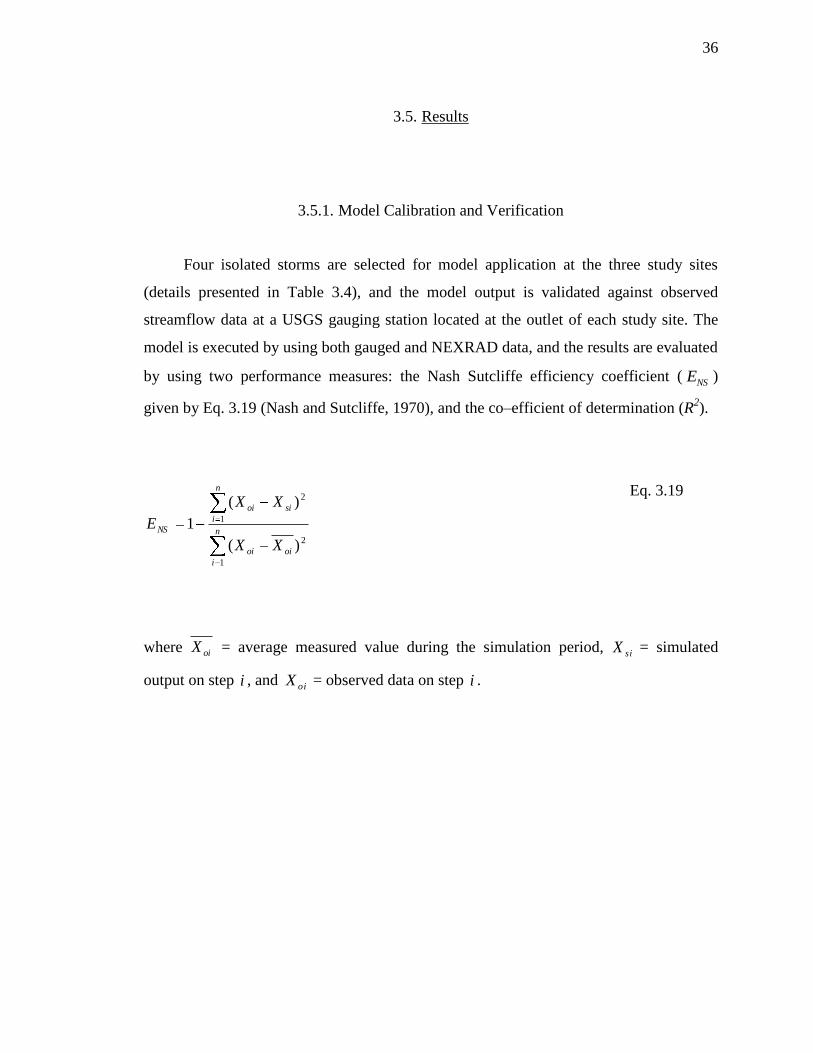
3.5.1. Model Calibration and Verification

Four isolated storms are selected for model application at the three study sites

(details presented in Table 3.4), and the model output is validated against observed

streamflow data at a USGS gauging station located at the outlet of each study site. The

model is executed by using both gauged and NEXRAD data, and the results are evaluated

by using two performance measures: the Nash Sutcliffe efficiency coefficient (NSE )

given by Eq. 3.19 (Nash and Sutcliffe, 1970), and the co–efficient of determination (R2).

n

i

oioi

n

i

sioi

NS

XX

XX

E

1

2

1

2

)(

)(

1

Eq. 3.19

where oiX = average measured value during the simulation period, siX = simulated

output on step i , and oiX = observed data on step i .

37

Table 3.4 Details of storm events for each site.

Study

Site

Event

#

Start Date

and Time

Time

Step

(hr)

Total Precipitation

(mm) Total

Streamflow

(mm)

Peak

Flow

(m3/s)

Time

to

Peak

(hr) Gauge NEXRAD

Cedar

Creek

1 05–02–02,

00:00 1.00 7.68 8.49 4.79 23.36 30.0

2 05–02–21,

01:00 1.00 9.46 8.86 6.32 27.30 26.0

3 05–03–19,

16:00 0.50 8.89 8.94 2.88 12.80 17.5

4 06–01–13,

22:00 0.25 17.10 16.99 3.91 24.95 14.5

Fish

Creek

1 05–01–12,

22:30 0.50 40.34 34.74 12.58 8.67 25.0

2 05–03–06,

13:30 0.50 11.39 14.71 3.37 2.10 28.5

3 06–01–02,

16:00 0.50 15.24 17.47 5.33 3.03 20.5

4 06–02–16,

08:30 0.50 20.39 21.17 4.64 3.34 27.0

Crooked

Creek

1 05–01–03,

14:45 0.25 45.72 38.25 15.93 28.07 7.5

2 05–01–11,

08:45 0.25 36.13 33.21 12.01 16.57 8.5

3 05–02–05,

12:45 0.25 31.56 31.39 6.21 7.39 11.5

4 05–02–13,

06:15 0.25 40.64 36.56 18.99 18.41 6.0

38

The STORE DHM is first executed without calibration for each study site using

rain gauge data for event 1 (C1, F1 and R1 in Table 3.5). The resulting hydrographs and

then properties are presented in Fig. 3.6 and Table 3.5. Un–calibrated results show that

the peak flow is underestimated by 30% for Cedar Creek, overestimated by 30% for Fish

Creek, and within less than 0.5% error for Crooked Creek. Similarly, the time–to–peak is

overestimated for Cedar Creek (10%) and Crooked Creek (33%) and underestimated for

Fish Creek (20%). Overall, the total run–off depth between the model output and

observed data looks reasonable for both Fish and Crooked Creek, and for Cedar Creek,

the model runoff is 20% lower than observed runoff. The Nash–Sutcliffe coefficient is

lower than 0.7 for all simulations. After the un–calibrated simulation for event 1, the

model is calibrated manually for the same event at each study site by treating Manning‟s

n as the calibration parameter. Calibrated values of Manning‟s n for each land use at each

study site are presented in Table 3.6.

Table 3.5 Uncalibrated models results for Event 1 at each study site (C is Cedar Creek, F

is Fish Creek and R is Crooked Creek.).

Area Runoff Depth

(mm)

Peak Flow

(m3/s)

Time to Peak

(hr) R

2 ENS

C1 3.915 16.340 33.0 0.72 0.57

F1 11.809 11.030 19.5 0.83 0.68

R1 14.889 27.080 10.0 0.65 0.63

39

0

5

10

15

20

25

0 25 50 75

C1 - Gauge

0

2

4

6

8

10

12

0 15 30 45 60

F1 - Gauge

Cedar Creek Fish Creek

0

5

10

15

20

25

30

0 3 6 9 12

R1 - Gauge

Crooked Creek

Figure 3.6 Uncalibrated model results for Event 1 (C1, F1 and R1) using gauged rainfall

input. X–axis represents time in hours and Y–axis represents flow in cubic meters per

second.

Observation STORE DHM

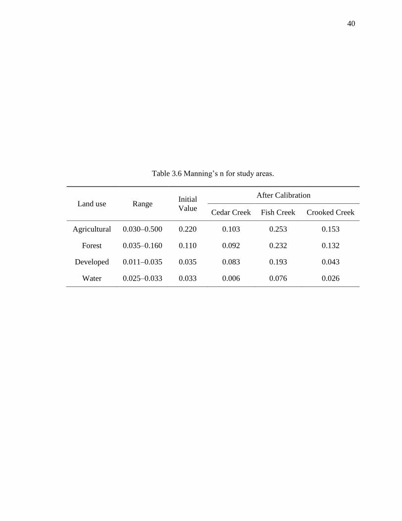
40

Table 3.6 Manning‟s n for study areas.

Land use Range Initial

Value

After Calibration

Cedar Creek Fish Creek Crooked Creek

Agricultural 0.030–0.500 0.220 0.103 0.253 0.153

Forest 0.035–0.160 0.110 0.092 0.232 0.132

Developed 0.011–0.035 0.035 0.083 0.193 0.043

Water 0.025–0.033 0.033 0.006 0.076 0.026

41

Table 3.7 Calibration and validation results for all events (1–4) for Cedar Creek (c), Fish

Creek (F) and Crooked Creek (R) using gauge rainfall.

Event

Simulation with Gauge Rainfall

Runoff Depth

(mm)

Peak Flow

(m3/s)

Time to Peak

(hr) R

2 ENS

C1 4.30 22.92 26.00 0.90 0.87

C2 6.03 36.00 26.00 0.92 0.78

C3 2.49 12.88 21.00 0.98 0.95

C4 3.08 23.89 14.50 0.95 0.85

F1 10.96 8.50 25.00 0.86 0.81

F2 2.93 1.97 14.00 0.89 0.82

F3 4.96 2.84 21.50 0.90 0.88

F4 5.05 3.29 29.00 0.90 0.87

R1 16.00 27.58 8.25 0.84 0.84

R2 10.95 17.12 9.75 0.91 0.89

R3 5.83 7.40 10.75 0.76 0.73

R4 15.15 19.87 7.25 0.91 0.87

42

Table 3.8 Calibration and validation results for all events (1–4) for Cedar Creek (c), Fish

Creek (F) and Crooked Creek (R) using NEXRAD rainfall.

Event

Simulation with NEXRAD Rainfall

Runoff Depth

(mm)

Peak Flow

(m3/s)

Time to Peak

(hr) R

2 ENS

C1 4.65 23.36 27.00 0.88 0.88

C2 4.88 28.27 23.00 0.94 0.83

C3 2.57 13.18 21.50 0.97 0.95

C4 3.10 24.26 11.00 0.74 0.64

F1 10.44 8.07 23.50 0.91 0.81

F2 3.61 1.87 24.50 0.83 0.81

F3 5.24 3.21 13.50 0.93 0.93

F4 5.57 3.14 27.00 0.80 0.70

R1 15.77 28.60 7.25 0.97 0.97

R2 9.98 14.74 8.00 0.94 0.85

R3 5.83 7.00 11.50 0.75 0.74

R4 12.48 17.80 7.75 0.84 0.71

43

0

5

10

15

20

25

0 20 40 60 80

C1 - Gauge

0

5

10

15

20

25

0 20 40 60 80

C1 - NEXRAD

0

10

20

30

40

0 20 40 60 80 100

C2 - Gauge

0

10

20

30

40

0 20 40 60 80 100

C2 - NEXRAD

0

3

6

9

12

15

0 25 50 75 100 125

C3 - Gauge

0

3

6

9

12

15

0 25 50 75 100 125

C3 - NEXRAD

0

5

10

15

20

25

30

0 15 30 45 60

C4 - Gauge

0

5

10

15

20

25

30

0 15 30 45 60

C4 - NEXRAD

Figure 3.7 Cedar Creek model hydrographs. X–axis represents time in hours and Y–axis

represents flow in cubic meters per second.

Observed STORE DHM

44

0

2

4

6

8

10

0 15 30 45 60

F1 - Gauge

0

2

4

6

8

10

0 15 30 45 60

F1 - NEXRAD

0.0

0.5

1.0

1.5

2.0

2.5

0 15 30 45 60 75

F2 - Gauge

0.0

0.5

1.0

1.5

2.0

2.5

0 15 30 45 60 75

F2 - NEXRAD

0

1

2

3

4

0 20 40 60 80

F3 - Gauge

0

1

2

3

4

0 20 40 60 80

F3 - NEXRAD

0

1

2

3

4

0 15 30 45 60 75

F4 - Gauge

0

1

2

3

4

0 15 30 45 60 75

F4 - NEXRAD

Figure 3.8 Fish Creek model hydrographs. X–axis represents time in hours and Y–axis


Observed STORE DHM

45

0

5

10

15

20

25

30

0 3 6 9 12

R1 - Gauge

0

5

10

15

20

25

30

35

0 3 6 9 12

R1 - Gauge

0

3

6

9

12

15

18

0 3 6 9 12 15

R2 - Gauge

0

3

6

9

12

15

18

0 3 6 9 12 15

R2 - NEXRAD

0

3

6

9

0 3 6 9 12 15 18 21 24 27

R3 - Gauge

0

3

6

9

0 3 6 9 12 15 18 21 24 27

R3 - NEXRAD

0

3

6

9

12

15

18

21

0 3 6 9 12 15 18 21

R4 - Gauge

0

3

6

9

12

15

18

21

0 3 6 9 12 15 18 21

R4 - NEXRAD

Figure 3.9 Crooked Creek model hydrographs. X–axis represents time in hours and Y–

axis represents flow in cubic meters per second.

Observed STORE DHM

46

After calibration using gauged rainfall, the model is applied to the same event

using NEXRAD input, and these results are presented in Tables 3.7 and 3.8. Tables 3.7

and 3.8 also present results from application of the model for three additional events at

each site using both rain gauge and NEXRAD rainfall input. Hydrographs corresponding

to results in Tables 3.7 and 3.8 are presented in Figs. 3.7–3.9 for each study site.

Qualitative and quantitative comparisons of each model hydrograph (peak flow, total

run–off depth and time–to–peak in Tables 3.7 and 3.8) with observed hydrograph show

reasonable agreement (Table 3.4). Two performance measures (R2 and ENS) used in this

study give a value of 0.8 or higher for most events included in this study with an average

R2 and ENS of 0.88 for Cedar Creek, 0.85 for Fish Creek, and 0.85 for Crooked Creek.

Regardless of the values of performance measures, the differences between observed data

and model results including the differences between gauged and NEXRAD output can be

attributed to the overall modeling approach and the quality of the input data.

3.5.2. Comparison with HEC–HMS

In addition to calibrating and validating the STORE DHM against independent

storm events, the model results are compared with another event based model, HEC–

HMS, for storm events in Cedar Creek. The HEC–HMS model for Cedar Creek also uses

the SCS curve number method for computing excess rainfall, and the excess rainfall is

transformed to the runoff hydrograph using the Clark Unit Hydrograph method. The

routing through river channels is simulated by using the simple lag method. The Clark

unit hydrograph method has two parameters (Time of Concentration and Storage

Coefficient), and the lag method has one parameter (Lag time). Thus, the HEC–HMS

simulations used in this study involve three parameters. Similar to STORE DHM, HEC–

HMS is calibrated for these three parameters by using the data for the first storm event.

The calibrated model is then validated by conducting simulations for three additional

storm events in Cedar Creek. Table 3.9 presents a summary of model results and error

47

statistics for HEC–HMS simulations. Excluding the calibration results for event 1, HEC–

HMS over estimates the peak discharge by 40% for Event 2 to more than 200% for event

3 (Fig. 3.10). The time–to–peak is underestimated for events 2 and 4, and overestimated

for event 3. Results for events 3–4 are particularly discouraging from HEC–HMS in

terms of the overall hydrograph shape and run–off volume.

Table 3.9 HEC–HMS model results for Cedar Creek.

Event

HEC– HMS Simulation with Gauged Rainfall

Runoff Depth

(mm) Peak Flow (m

3/s)

Time to Peak

(hr) R

2 ENS

C1 4.49 22.86 24.00 0.94 0.92

C2 8.98 37.09 21.00 0.85 0.18

C3 17.60 37.04 16.50 0.86 –9.66

C4 51.24 62.61 21.25 0.05 –16.53

48

0

5

10

15

20

25

0 15 30 45 60 75

C1 - Gauge

0

10

20

30

40

0 20 40 60 80 100

C2 - Gauge

0

10

20

30

40

0 35 70 105 140

C3 - Gauge

0

10

20

30

40

50

60

70

0 25 50 75 100 125

C4 - Gauge

Figure 3.10 Comparison of HEC–HMS and STORE DHM hydrographs with observed

data for Cedar Creek. X–axis represents time in hours and Y–axis represents flow in

cubic meters per second.

Observed HEC–HMS STORE DHM

49

3.5.3. Comparison with time variant SDDH Model

The results from the STORE DHM are compared with the grid based time variant

spatially distributed direct hydrograph travel time method (SDDH) by Du et al. (2009).

The methodology for this comparison is similar to that of HEC–HMS and involves

calibration of the time variant SDDH model using the first storm event, and validation

using the next three storm events. The velocity needed to compute the travel time in time

variant SDDH is given by Eq. 3.20, which involves a parameter K that is determined

through calibration. Through manual calibration of the model for Event 1, a value of 6.5

was determined for K, and used in subsequent simulations.

3/8 1/4 3/4

0V Ks Q n Eq. 3.20

where V is velocity in m/s, Q is discharge m3/s, s0 is the channel slope, and n is

Manning‟s coefficient. Results (Fig. 3.11 and Table 3.10) show that time variant SDDH

over estimates both peak discharge and time–to–peak for events 2–4 compared to the

observed flow. The overestimation of peak discharge ranges from 15% for event 4 to

50% for event 2. Similarly, the time–to–peak is overestimated in the range of 10% for

event 4 to 50% for event 2.

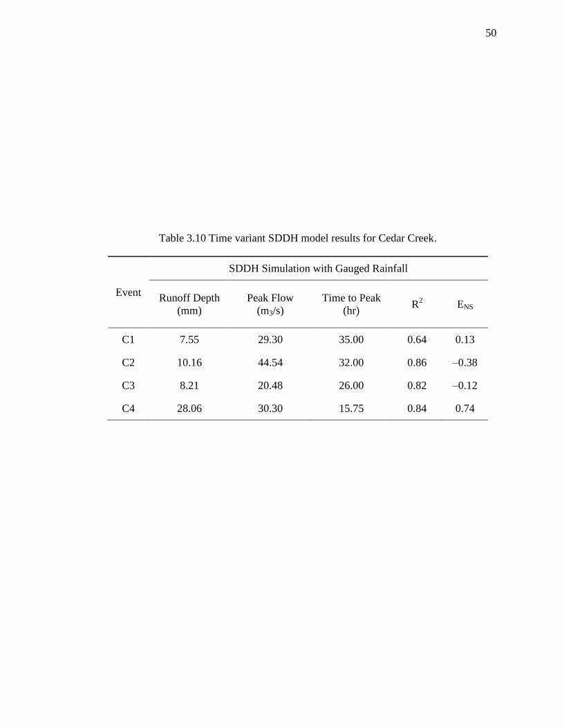
50

Table 3.10 Time variant SDDH model results for Cedar Creek.

Event

SDDH Simulation with Gauged Rainfall

Runoff Depth

(mm)

Peak Flow

(m3/s)

Time to Peak

(hr) R

2 ENS

C1 7.55 29.30 35.00 0.64 0.13

C2 10.16 44.54 32.00 0.86 –0.38

C3 8.21 20.48 26.00 0.82 –0.12

C4 28.06 30.30 15.75 0.84 0.74

51

0

5

10

15

20

25

30

0 15 30 45 60 75

C1 - Gauge

Obs

SDDH

STORE DHM

0

10

20

30

40

50

0 25 50 75 100

C2 - Gauge

0

5

10

15

20

0 35 70 105 140

C3 - Gauge

0

5

10

15

20

25

30

35

0 35 70 105

C3 - Gauge

Figure 3.11 Comparison of time variant SDDH and STORE DHM hydrographs with

observed data for Cedar Creek. X–axis represents time in hours and Y–axis represents

flow in cubic meters per second.

Observed SDDH STORE DHM

52

3.6. Discussion

The storage release approach used in this study is dependent mainly on the travel

time, which in turn is dependent on Manning‟s n. The fact that the model is calibrated

using only one parameter is attractive from a practical point of view, but it sometimes

becomes difficult to get both the peak flow and the time–to–peak to match with observed

data. The error in peak flow for all simulations is much smaller compared to the error in

time–to–peak. For example, the average percentage error in peak flow for Cedar Creek,

Fish Creek and Crooked Creek is 7.8%, 4.2%, and 3.1%, respectively. The average

percentage error in time–to–peak for Cedar Creek, Fish Creek and Crooked Creek is

8.0%, 28.8%, and 11.5%, respectively. Inclusion of more parameterized approaches for

computing excess rainfall (or losses) such as the Green–Ampt Method may provide more

flexibility in modeling hydrographs, but these options are still under development, and

are not tested in this study.

Radar precipitation estimates are obtained by converting reflectance (Z) into

precipitation (R) by using Z–R relationship (Smith, 1986). The Z–R relationship has

uncertainties that affect the estimated radar precipitation, and in general, radar estimates

tend to be different from rain gauge data. NEXRAD data attempts to reduce this

difference by assimilating rain gauge data into radar precipitation estimate, but still some

differences remain between rain gauge data and radar precipitation as evident from

results in Table 3.4. For example in Crooked Creek watershed, which is mostly urban,

total NEXRAD precipitation estimates are significantly lower compared to rain gauge

data for three storm events (R1, R2 and R4); whereas for Fish Creek watershed (rural)

NEXRAD precipitation estimates are higher than gauged data. Despite these differences

in the input data, the overall model hydrograph shape is not different for both gauged and

NEXRAD input (Figs. 3.7–3.9), but the total runoff depth (or volume) is different as

shown in Tables 3.7 and 3.8.

The storage release approach in the STORE DHM does seem to capture the spatial

distribution of rainfall as evident in C1 and C2 for Cedar Creek. In the case of C1, it

seems that the rainfall was more uniformly distributed over the area thus giving

53

reasonable hydrographs for both gauged and NEXRAD. However for C2, higher rainfall

recorded at the gauge yields higher runoff volume and peak (Fig. 3.7–C2), but the

NEXRAD hydrograph matches well with observed data, thus suggesting that the rainfall

observed at the gauge was higher than the average rainfall in the watershed. Similarly, the

storage release approach seems to capture the bimodal nature of hydrographs observed in

Crooked Creek watershed (Figs.3.9–R1 and 3.9–R3). The results with NEXRAD input

are relatively better compared to gauged input for bimodal hydrographs. If it is assumed

that NEXRAD precipitation provides better representation of the spatial distribution of

rainfall in a watershed, then simulation results using Multisensor Precipitation Estimators

(MPE) data should provide better output compared to the output from gauge rainfall in

terms of peak flow and time–to–peak, which are important attributes in event based

modeling. The results, however, show that output from MPE are not always better in

terms of predicted peak flow and time–to–peak for some events compared to gauged data.

These events include C4, F1, F2, F4, R1, R2 and R4 for peak flow as well as C2, C3, C4,

F1, F3 and R4 for time to peak.

The inability of HEC–HMS to produce reasonable results for all Cedar Creek

simulations (Fig. 3.10) is understandable considering that the hydrograph (C1) that was

used for its calibration has different characteristics (e.g., shape, duration and flow peak)

compared to the other three events (C2–C4) used for its verification. Similarly, although

the output from time variant SDDH for Cedar Creek simulations is better compared to

HEC–HMS, the peak flow is over estimated by time variant SDDH for all simulations.

Comparison of STORE DHM with both HEC–HMS and time variant SDDH

demonstrates its robustness in simulating different types of events with consistent results.

This robustness of STORE DHM can be attributed to its dependence on only one

parameter (Manning‟s n), which retains its physical meaning (representation of surface

roughness) in all simulations, and the selection of model time step using the concept of

critical cell travel time.

54

3.7. Conclusions and Future Work

The conceptual framework and application of a grid–based model, the STORE

DHM, using the storage–release concept is presented in this study. Results show that the

STORE DHM is able to simulate the hydrologic behavior of a watershed to produce

streamflow hydrographs that match well with observed data. In addition, the STORE

DHM is able to ingest both point and distributed rainfall input, and the comparison of

outputs from these two types of inputs show that the storage–release approach is able to

capture the rainfall dynamics in the NEXRAD data. Unlike other raster or grid–based

models that route the flow from each cell to the watershed outlet along a common flow

path at each time step (which can lead to improper water balance), the STORE DHM

considers the flow contribution of neighboring cells by using the simple continuity

equation (change in storage = input – output). This simplicity in turn provides

computational efficiency, which is critical for real–time hydrologic forecasting. Similarly,

the STORE DHM is a part of the broader GHISMO framework that provides flexibility in

modular development of the model without changing the basic framework. For example,

Chapter 4 presents a module to correct the bias (due to Z–R conversion and limited rain

gauges information) in Multisensor Precipitation Estimator (MPE) NEXRAD data by

developing an object for assimilating multiple data sources to get robust rainfall input.

The modeling framework presented in this chapter is operated within ArcGIS

environment such that all the steps from extracting information from geospatial data to

running model simulations are executed in ArcGIS environment. The approach from data

to model output within a single environment is attractive from a practical point of view.

Although the prototype modeling approach and its application including comparison with

HEC–HMS and time variant SDDH is encouraging, there are several issues that still need

to be addressed for this modeling framework to be fully useful for practical applications.

These issues include: (i) testing the scalability of the model by applying it to larger

watersheds (with more than 1,000 km2 area) including regional basins (with areas in the

range of several 10,000 km2); (ii) investigation of computational efficiency and simplicity

with multiple runoff generation mechanisms (e.g., Green–Ampt) and parameters; (iii)

55

ability of the model to ingest near real–time spatial (remote sensing) and temporal data

for hydrologic modeling; and (iv) creating a protocol through which existing research

codes can be converted to objects that can be incorporated into GHISMO.

56

CHAPTER 4. IMPROVING RAINFALL ACCURACY ON DISTRIBUTED

HYDROLOGIC MODELING BY USING SPATIALLY UNIFORM AND NON–

UNIFORM NEXRAD BIAS CORRECTION

4.1. Introduction

Representation of rainfall dynamics plays a critical role in making accurate

hydrologic predictions. Numerous studies in the past decades have investigated the

sensitivity of runoff hydrographs to rainfall by using gauged data. In addition to the

accuracy of gauged rainfall input, the predictability and sensitivity of hydrologic models

are dependent on the spatio–temporal representation of rainfall (Faures et al. 1995;

Wilson et al. 1979; Troutman et al. 1989). To overcome these limitations, radar rainfall

data are increasingly used in hydrologic applications (Smith et al., 2004). The next

generation radar (NEXRAD) products available from 1992 provide high resolution

rainfall information in space and time. Currently, the NEXRAD precipitation products

are categorized into four levels according to the amount of preprocessing, calibration, and

quality control performed. The StageI product is an hourly digital precipitation (HDP)

directly derived from reflectivity measurements using a Z–R (reflectivity–rainfall)

relationship after the application of several quality control algorithms (e.g. Fulton et al.,

1998). StageII is the single radar site HDP product, which is merged with surface rain

gauge observations to correct mean field bias using Kalman filtering (Smith and

Krajewski, 1991; Anagnostou et al., 1999). In StageIII, the StageII rainfall data from

multiple weather radars covering a River Forecast Center (RFC) region are combined

(Fulton et al., 1998; Reed and Maidment, 1999). Finally, StageIV is the mosaicked

StageIII rainfall product covering the entire Continental United States (CONUS).

57

The most commonly used NEXRAD product in hydrometeorological applications

is the NEXRAD StageIII data (e.g. Young et al., 2000) since it involves the correction of

radar rainfall rates with multiple surface rain gauges and has a significant degree of

metrological quality control by trained personnel at individual RFCs (Fulton et al., 1998).

Since around 2002, Multisensor Precipitation Estimator (MPE), which are developed by

the National Weather Service (NWS) Office of Hydrology, is available for each RFC.

The MPE product is obtained by merging radar, gauge and satellite estimates of rainfall

and is adjusted for mean field and local biases. In spite of better spatial representation of

rainfall variability by radar, there are limitations of radar estimates due to data

contamination and uncertainty issues (Smith et al., 1996; Legates, 2000; Xie et al., 2006).

In particular, uncertainty in radar rainfall is caused by reflectivity–rainfall conversion

method, limitation of available rain gauge information for mean field bias adjustment and

spatially uniform bias correction for entire RFCs. Minimizing errors in radar precipitation

has been one of the major tasks in hydrologic and meteorologic research for decades

(Schimid and Wuest, 2005).

An intense topic of water resources research has been merging radar and gauge

rainfall to estimate a high accuracy rainfall. Smith and Krajewski (1991) found that

combining radar and gauge information produces improved precipitation estimates, in

terms of both quality and spatial resolution, in comparison with either radar or gauge

estimates alone. Krajewski (1987), Pereira et al. (1998) and Seo (2002) proposed co–

kriging, statistical objective analysis and Kalman filtering approach, respectively.

However, uncertainty persists in radar precipitation products because large portions of

radar coverage areas do not have rain gauge data to adjust biases in radar rainfall

(Winchell et al., 1998; Habib et al., 2009). The different radar rainfall error correction

schemes in mountainous areas are investigated by Dinku et al. (2002). Correction for

terrain blocking, adjustment for rain attenuation, and interpolation of reflectivity data are

used for radar rainfall error correction. They also used a Kalman filtering–based mean

field radar bias correction scheme that is similar to the approach of the Anagnostou and

58

Krajewski (1998) study. They found that adjustment of radar bias with the filtering

approach produced extremely high accuracy radar rainfall.

In NEXRAD StageIII (MPE), analysis bias in radar rainfall is corrected using

available rain gauges. The correction procedures assume that the biases are spatially

uniform over the entire RFC region. These spatially uniform biases are referred to as

mean field bias (Smith and Krajewski, 1991). However, recent studies have shown that

the assumption of spatially uniform bias is not valid over particular regions (Li et al.,

2010). The NEXRAD rainfall bias over a small watershed in an RFC region could be

very different from the mean bias over the entire RFC region. Looper et al. (2009)

concluded that even though MPE already takes radar bias correction, the resulting

precipitation may not be accurate for a particular river basin, because adjustment is

performed on the entire RFC region. Consequently, hydrologic model simulations for a

particular watershed with MPE analysis data could be unrealistic. Nevertheless, the effect

of these spatially non–uniform local biases on hydrologic simulations is not well

understood (Li et al., 2010). Further, the few methods that are available to correct

spatially non–uniform local biases (Seo et al., 2001) have limitations such as limited

number of rain gauge data for correcting local radar biases, and their sensitivity to

hydrologic model simulations has not been tested.

Literature shows that the availability of high–resolution precipitation data from

different weather radar platforms has led to improved understanding of rainfall

uncertainty in hydrologic models, but few efforts have been directed towards

understanding the influence of NEXRAD precipitation and its bias correction on rainfall–

runoff simulations. This study presents three different NEXRAD rainfall bias correction

schemes and their influence on sensitivity of grid based distributed hydrologic model

simulations.

59

4.2. Study Areas and Data

The Upper Wabash River and the Upper Cumberland River (Fig. 4.1) basins are

selected as the test beds for this study. In addition to providing two distinct geographic

locations, both study areas include a reasonable rain gauge network to compare bias

correction schemes using NEXRAD data. The Upper Wabash River basin (UWR; 17,907

km2) is located in north central Indiana, and it drains into the Wabash River. The

elevation in UWR ranges from 149 to 529 m. Normal annual precipitation of the UWR

ranges between 920 and 1120 mm as computed by using data from 17 rain gauges in the

region. The Upper Cumberland River basin (UCR; 38,160km2) is located in southeastern

Kentucky bordering with Virginia and Tennessee. The UCR is primarily mountainous

and forested, and it lies in the Eastern Coal Field physiographic region. The elevation in

the UCR ranges from 146 to 1428 m. Normal annual precipitation of the UCR ranges

from 950 to 1300mm as computed from 19 rain gauges in the region.

The NEXRAD rainfall dataset for the study area is distributed by HRAP

(Hydrologic Rainfall Analysis Project) geographic projection. The HRAP or secant polar

stereographic projection is an earth–centered datum coordinate system. Reed and

Maidment (1995, 1999) describe the HRAP projection and its transformations to other

geodetic coordinate systems. The NEXRAD StageIII data are converted to re–projecting

ASCII by using C++ program for conversion of XMRG (binary) file format to ASCII,

and conversion of ASCII data to GIS grid format by first defining the HARP projection

to the desired coordinate system. Rain gauge measurements of five storms recorded on

February, April, July, October and November, 2006 for the UWR and January, February,

March, April and July, 2005 for the UCR are selected for this study. The observational

networks of NEXRAD StageIII, rain gauges, and stream gauges that cover the UWR and

the UCR basins are shown in Fig. 4.2, and Table 4.1 displays summary of rainfall event

for each site.

60

Figure 4.1 Study basin locations in relation to rain gauges and stream gauges (UWR –

Upper Wabash River basin, UCR – Upper Cumberland River basin).

61

Figure 4.2 Basin locations and surrounding NEXRAD StageIII.

62

Table 4.1 Summary of storm events for application of NEXRAD bias correction.

Event

Upper Wabash River

Basin

Upper Cumberland River

Basin

Start Date and Time Start Date and Time

1 06–02–17, 01:00 05–01–11, 12:00

2 06–04–16, 19:00 05–02–13, 10:00

3 06–07–12, 03:00 05–03–27, 23:00

4 06–10–27, 19:00 05–04–01, 18:00

5 06–11–16, 08:00 05–07–13, 08:00

63

4.3. NEXRAD Bias Correction Methods

A statistical method should be used to remove the bias between NEXRAD

estimates at the rain gauge locations, and corresponding gauge rainfall measurements

because NEXRAD rainfall estimates have errors from reflectivity measurement and the

Z–R conversion. To test the sensitivity of NEXRAD bias correction on runoff

hydrographs, three methods based on the Kalman filter are used in this study. The first

method is based on application of spatially uniform bias correction as used in MPE data.

The second and third methods are based on the application of spatially non–uniform bias

correction. A brief description of Kalman Filter and its application for spatially and non–

spatially uniform bias correction is presented below.

4.3.1. Kalman filter

The Kalman filtering equations have two series of stages, which are time update

and measurement update, to estimate the best possible bias. Projecting forward (in time)

the current state is performed in time update. Correcting new a priori estimate at the

current time step is performed in measurement update (Welch and Bishop, 2001).

(1) Discrete Kalman filter Time update

According to Smith and Krajewski (1991), NEXRAD bias ( ) is assumed as an

Autoregressive order one (AR1) process whose parameters are updated using a Kalman

filter as given by Eq. 1.

( )t = ( 1) ( )t W t ; ( ) ~ (0, )W t Eq. 4.1

64

where ( )t is NEXRAD bias for hour t, is lag–one correlation coefficient of the

logarithmic bias, and W(t) is a sequence of independent normally distributed random

variables with mean zero and variance . The stationary process variance ( ) and the

stationary variance of the log bias process (2) are given by Eqs. 4.2 and 4.3.

= 22

)1( . Eq. 4.2

2 ( )Var t ; t = 0, …., T Eq. 4.3

where T is storm duration.

The a priori estimate of can be estimated using Eq. 4.4.

( )t = ( 1)t Eq. 4.4

where takes into account the new measurement that is observed, and corrects for any

errors that may be present in the newly measured value.

The process variance ( ( )P t ) is estimated using Eq. 4.5.

( )P t = 2 2 2( 1) (1 )P t Eq. 4.5

where P(t–1) is the a posteriori estimate error variance at time t–1. The initial value of

0 and P0 are zero and

2, respectively.

(2) Discrete Kalman filter Measurement update

In each time and measurement update pair, the process is repeated with the

previous a posteriori estimates used to project or predict the new a priori estimates. This

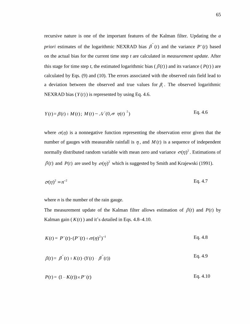
65

recursive nature is one of the important features of the Kalman filter. Updating the a

priori estimates of the logarithmic NEXRAD bias ( )t and the variance ( )P t based

on the actual bias for the current time step t are calculated in measurement update. After

this stage for time step t, the estimated logarithmic bias ( ( )t ) and its variance ( ( )P t ) are

calculated by Eqs. (9) and (10). The errors associated with the observed rain field lead to

a deviation between the observed and true values fort. The observed logarithmic

NEXRAD bias ( ( )Y t ) is represented by using Eq. 4.6.

( )Y t = ( ) ( )t M t ; 2

( ) ~ (0, ( ) )M t t Eq. 4.6

where ( ) is a nonnegative function representing the observation error given that the

number of gauges with measurable rainfall is , and ( )M t is a sequence of independent

normally distributed random variable with mean zero and variance 2( ) . Estimations of

( )t and ( )P t are used by 2( ) which is suggested by Smith and Krajewski (1991).

2 2( ) n Eq. 4.7

where n is the number of the rain gauge.

The measurement update of the Kalman filter allows estimation of ( )t and ( )P t by

Kalman gain ( ( )K t ) and it‟s detailed in Eqs. 4.8–4.10.

( )K t = 2 1( ) ( ( ) ( ) )P t P t Eq. 4.8

( )t = ( ) ( ) ( ( ) ( ))t K t Y t t Eq. 4.9

( )P t = (1 ( )) ( )K t P t Eq. 4.10

66

Due to the bias model defined in terms of the log bias process, Smith and Krajewski

(1991) suggest Eq. 4.11 for state expectation of the bias correction factor at the time t as

shown below

( )B t = ( ) 0.5 ( )

10t P t

. Eq. 4.11

4.3.2. Spatially uniform NEXRAD Bias Correction using Kalman filter

According to Seo et al. (1999) and Dinku et al. (2002), mean field bias corrections

and vertical profile of reflectivity adjustments are needed to correct spatially uniform

biases in NEXRAD data. The variance of the observed mean field bias should affect the

magnitude of the Kalman filter observation error model. The time–dependent variance of

the observed mean field bias (MFB) is estimated by using the variance of logarithmic

bias proposed by Smith and Krajewski (1991). The correction procedures assume that the

biases are spatially uniform over the entire study area. The logarithmic MFB between

NEXRAD estimates at the rain gauge locations and the corresponding gauge rainfall

amounts is computed by equation 4.12.

( )t = 10

1

10

1

1log ( ( ) )

1log ( ( ) )

n

i

i

n

i

i

G tn

R tn

Eq. 4.12

where G(t)i is hourly rain gauge rainfall at NEXRAD–gauge paired cell i for hour t, R(t)i

is hourly NEXRAD rainfall at NEXRAD–gauge paired cell i for hour t, and n is the

number of radar–gauge pairs data available for an hour. The spatially uniform bias

corrected NEXRAD rainfall is then computed by using Eq. 4.13.

67

*( ) ( ) ( )j jR t B t R t Eq. 4.13

where R*(t)j is bias corrected NEXRAD at j location at time t, and R(t)j is hourly

NEXRAD rainfall at gauge cell j for hour t within the study area.

4.3.3. Spatially non–uniform NEXRAD Bias Correction using Kalman Filter

In the spatially uniform bias correction method, the radar bias (Eq. 4.12) over the

cells with observed rain gauge data is assumed to be uniform for all NEXRAD cells

without corresponding rain gauges. The assumption of uniform bias may or may not be

true depending on the rainfall dynamics and the size of the watershed. As a result, the

bias may be higher for NEXRAD cells that do not overlap with rain gauge locations. In

order to minimize such un–gauged NEXRAD cell bias, this study suggests application of

a spatially non–uniform bias correction using Kalman filter. Unlike the MFB (Eq. 4.12),

the spatially non–uniform biases vary from pixel to pixel across the NEXRAD domain.

The corrected NEXRAD rainfall at an un–gauged NEXRAD pixel j for hour t, R*(t)j, is

computed by multiplying spatially non–uniform bias correction factor (B(t)j) at each un–

gauged NEXRAD grid location j using Eq. 4.14.

*( ) ( ) ( )j j jR t B t R t Eq. 4.14

There are two approaches for computing the spatially non–uniform bias. In the first

approach, the rain gauge data are interpolated to get interpolated rainfall estimates for

un–gauged NEXRAD pixels. The squared inverse distance weighting (IDW) method (Eq.

4.15) is used for interpolation. Compared with other methods like Kriging, even though

68

its method consists of simple approach, it provides flexibility enough to predict the

variables with small size datasets in storm period (Adisoma and Hester, 1995).

* 1

1

( )

( )

n

i i

ij n

i

i

w G t

G t

w

Eq. 4.15

where G*(t)j is interpolated gauge information at un–gauged NEXRAD pixel j for hour t,

and wi (Eq. 4.16) is the weight corresponding to each gauged point.

0

1/

1/

b

ii n

b

i

i

dw

d

Eq. 4.16

where di is the distance between a radar pixel and the ith

rain gauge, b is an empirical

exponent and n is the number of rain gauges. The spatially non–uniform local NEXRAD

biases can then be estimated and corrected by using the interpolated rainfall (Eq. 4.17).

*

10

10

log ( ( ) )( )

log ( ( ) )

j

j

j

G tt

R t

Eq. 4.17

where ( ) jt is logarithmic local bias at un–gauged NEXRAD pixel j for hour t within the

study area.

In the second approach for applying non–uniform bias, the error at each gauged location

is computed using Eq. 4.18.

10

10

log ( ( ) )( )

log ( ( ) )

ii

i

G te t

R t

Eq. 4.18

69

The errors at each ith

gauge are then interpolated to get errors at all ungauged NEXRAD

pixels using squared inverse distance weighing. Ware (2005) found that the interpolation

errors associated with this IDW are comparable to those obtained using the multi–quadric

interpolation (Nuss and Titley, 1994) and ordinary kriging. An un–gauged NEXRAD bias

for spatially non–uniform bias correction is computed based on surrounding ratios and

distance of each gauge from the selected grid (Eq. 4.19).

1

1

( )

( )

n

i i

ij n

i

i

w e t

t

w

Eq. 4.19

where ( ) jt is logarithmic local bias at un–gauged NEXRAD pixel j for hour t within the

study area.

4.4. Results

Results are presented in two sections. In the first section, the quality of NEXRAD

data is assessed through cross–validation with observed rainfall. The NEXRAD data used

in cross–validation is prepared by using the spatially uniform bias correction method

(MPE), spatially non–uniform bias correction method by interpolating rainfall data

(SNU–R), and spatially non–uniform bias correction method by interpolating errors

(SNU–E). In the second section, the sensitivity of the STORE DHM hydrograph outputs

to rainfall created by using spatially uniform and non–uniform bias correction is

presented.

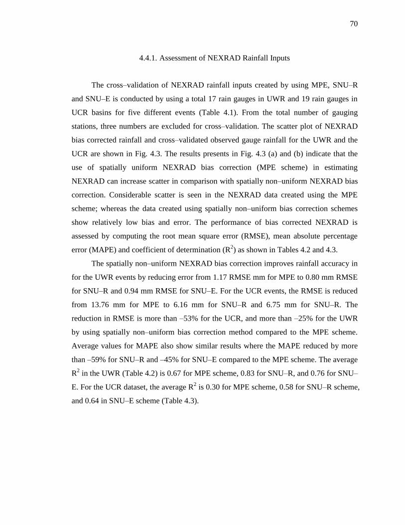
70

4.4.1. Assessment of NEXRAD Rainfall Inputs

The cross–validation of NEXRAD rainfall inputs created by using MPE, SNU–R

and SNU–E is conducted by using a total 17 rain gauges in UWR and 19 rain gauges in

UCR basins for five different events (Table 4.1). From the total number of gauging

stations, three numbers are excluded for cross–validation. The scatter plot of NEXRAD

bias corrected rainfall and cross–validated observed gauge rainfall for the UWR and the

UCR are shown in Fig. 4.3. The results presents in Fig. 4.3 (a) and (b) indicate that the

use of spatially uniform NEXRAD bias correction (MPE scheme) in estimating

NEXRAD can increase scatter in comparison with spatially non–uniform NEXRAD bias

correction. Considerable scatter is seen in the NEXRAD data created using the MPE

scheme; whereas the data created using spatially non–uniform bias correction schemes

show relatively low bias and error. The performance of bias corrected NEXRAD is

assessed by computing the root mean square error (RMSE), mean absolute percentage

error (MAPE) and coefficient of determination (R2) as shown in Tables 4.2 and 4.3.

The spatially non–uniform NEXRAD bias correction improves rainfall accuracy in

for the UWR events by reducing error from 1.17 RMSE mm for MPE to 0.80 mm RMSE

for SNU–R and 0.94 mm RMSE for SNU–E. For the UCR events, the RMSE is reduced

from 13.76 mm for MPE to 6.16 mm for SNU–R and 6.75 mm for SNU–R. The

reduction in RMSE is more than –53% for the UCR, and more than –25% for the UWR

by using spatially non–uniform bias correction method compared to the MPE scheme.

Average values for MAPE also show similar results where the MAPE reduced by more

than –59% for SNU–R and –45% for SNU–E compared to the MPE scheme. The average

R2 in the UWR (Table 4.2) is 0.67 for MPE scheme, 0.83 for SNU–R, and 0.76 for SNU–

E. For the UCR dataset, the average R2 is 0.30 for MPE scheme, 0.58 for SNU–R scheme,

and 0.64 in SNU–E scheme (Table 4.3).

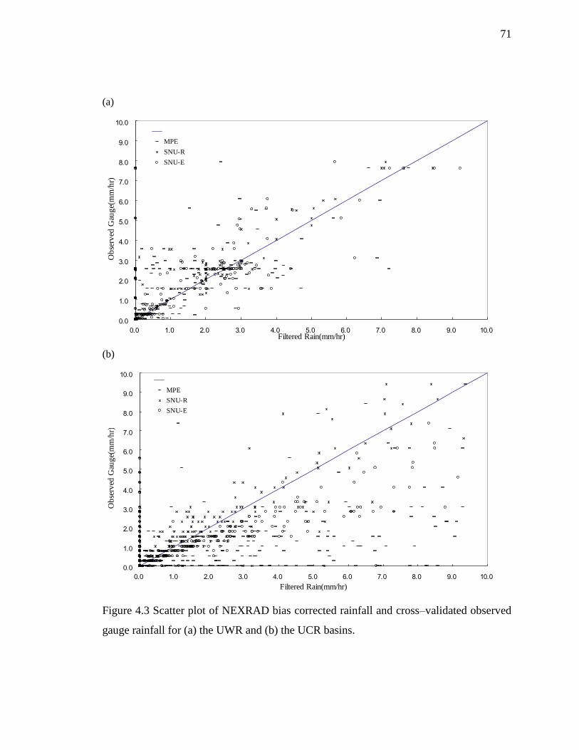
71

(a)

0.0

1.0

2.0

3.0

4.0

5.0

6.0

7.0

8.0

9.0

10.0

0.0 1.0 2.0 3.0 4.0 5.0 6.0 7.0 8.0 9.0 10.0Filtered Rain(mm/hr)

Ob

serv

ed G

aug

e(m

m/h

r)

MPE

SNU-R

SNU-E

(b)

0.0

1.0

2.0

3.0

4.0

5.0

6.0

7.0

8.0

9.0

10.0

0.0 1.0 2.0 3.0 4.0 5.0 6.0 7.0 8.0 9.0 10.0

Filtered Rain(mm/hr)

Ob

serv

ed G

aug

e(m

m/h

r)

MPE

SNU-R

SNU-E

Figure 4.3 Scatter plot of NEXRAD bias corrected rainfall and cross–validated observed

gauge rainfall for (a) the UWR and (b) the UCR basins.

72

Table 4.2 NEXRAD bias corrected rainfall statistics in the UWR basin.

Event

MPE scheme SNU–R scheme SNU–E scheme

RMSE

(mm)

MAPE

(%) R

2

RMSE

(mm)

MAPE

(%) R

2

RMSE

(mm)

MAPE

(%) R

2

1 0.80 12.06 0.74 0.59 8.05 0.87 0.71 9.98 0.80

2 1.73 48.13 0.57 0.76 18.76 0.92 1.09 31.07 0.82

3 1.63 30.72 0.62 1.46 14.40 0.70 1.44 17.56 0.70

4 0.38 22.00 0.89 0.13 10.28 0.98 0.26 17.73 0.93

5 1.30 93.41 0.53 1.05 19.04 0.67 1.21 66.79 0.57

Ave. 1.17 41.26 0.67 0.80 14.11 0.83 0.94 28.63 0.76

Table 4.3 NEXRAD bias corrected rainfall statistics in the UCR basin.

Event

MPE scheme SNU-R scheme SNU-E scheme

RMSE

(mm)

MAPE

(%) R

2

RMSE

(mm)

MAPE

(%) R

2

RMSE

(mm)

MAPE

(%) R

2

1 3.27 80.37 0.35 1.02 15.45 0.88 2.08 30.27 0.93

2 5.15 169.69 0.37 0.59 29.37 0.60 0.99 45.27 0.85

3 29.48 90.38 0.01 26.47 26.34 0.04 26.64 34.88 0.01

4 16.66 127.66 0.13 1.84 23.93 0.53 2.04 36.74 0.53

5 14.23 108.64 0.67 0.88 25.70 0.90 2.02 41.60 0.88

Ave. 13.76 115.35 0.30 6.16 24.16 0.58 6.75 37.75 0.64

73

(a)

0

1

2

3

4

5

6

7

8

9

10

0 10 20 30 40 50 60 70 80 90

Time (hr)

Sta

nd

ard

Dev

iati

on

UpperWabash

UpperCumberland

(b)

0

1

2

3

4

5

6

7

8

9

10

0 10 20 30 40 50 60 70 80 90

Time (hr)

Var

iati

on

Figure 4.4 Time series of (a) Standard Deviation and (b) Variation.

74

4.4.2. Sensitivity of Hydrographs to NEXRAD Bias Correction Schemes

To study the sensitivity of model hydrograph to rainfall inputs obtained by using

three different approaches for NEXRAD bias correction, the STORE DHM model is

calibrated for each event for both watersheds. The model is manually calibrated by using

the Nash–Sutcliffe coefficient (ENS) for discharge and root mean square error (RMSE) for

the total runoff volume. The RMSE are defined as

2

1

( )n

i i

sim obs

i

RMSE Q Q Eq. 4.1

where Qsim is the simulated hourly streamflow, and Qobs is the observed hourly

streamflow. Calibration factors used to adjust the model and the corresponding parameter

values are presented in Tables 4.4 and 4.5. The results from calibration are presented in

Figure 4.5 and Tables 4.6 and 4.7.

Table 4.4 Calibrated Manning‟s n values for each event in the UWR basin.

Event

Upper Wabash River Basin

Land Use Calibration

Agricultural Forest Developed Water

1 0.023 0.013 0.011 0.006

2 0.020 0.019 0.015 0.005

3 0.019 0.014 0.011 0.006

4 0.025 0.020 0.018 0.006

5 0.018 0.015 0.013 0.005

75

Table 4.5 Calibrated Manning‟s n values for each event in the UCR basin.

Event

Upper Cumberland River Basin

Land Use Calibration

Agricultural Forest Developed Water

1 0.051 0.035 0.033 0.016

2 0.081 0.055 0.043 0.026

3 0.061 0.036 0.023 0.020

4 0.062 0.043 0.037 0.012

5 0.054 0.037 0.035 0.015

76

0

20

40

60

80

100

120

140

160

180

200

0 20 40 60 80 100 120 140 160 180

Obs.

NEXRAD_Calibration

UWR1

0

5

10

15

20

25

30

35

40

45

0 20 40 60 80 100 120 140 160 180 200

Obs.

NEXRAD_Calibration

UWR1

0

50

100

150

200

250

300

350

400

450

0 20 40 60 80 100 120

Obs.

NEXRAD_Calibration

UWR2

0

20

40

60

80

100

120

140

160

180

200

0 20 40 60 80 100 120

Obs.

NEXRAD_Calibration

UWR2

0

50

100

150

200

250

300

350

400

0 20 40 60 80 100 120 140 160 180 200

Obs.

NEXRAD_Calibration

UWR3

0

50

100

150

200

250

0 20 40 60 80 100 120 140 160 180 200

Obs.

NEXRAD_Calibration

UWR3

0

50

100

150

200

250

300

350

0 50 100 150 200 250

Obs.

NEXRAD_Calibartion

UWR4

0

10

20

30

40

50

60

70

80

90

100

0 50 100 150 200 250

Obs.

NEXRAD_Calibration

UWR4

0

10

20

30

40

50

60

70

80

90

0 20 40 60 80 100 120 140 160 180 200

Obs.

NEXRAD_Calibration

UWR5

0

50

100

150

200

250

0 20 40 60 80 100 120 140 160 180 200

Obs.

NEXRAD_Calibration

UWR5

(a) UWR basin (b) UCR basin

Figure 4.5 Calibrated model results for every event using NEXRAD rainfall input (e.g.

UWR1 represents event 1 for UWR basin). X–axis represents time in hours and Y–axis


77

Table 4.6 Calibrated simulation statistics for each event in the UWR basin.

Event

Upper Wabash River Basin

Calibration with NEXRAD input

R2 ENS RMSE(m

3/s) MAPE(%)

1 0.98 0.97 2.21 14.58

2 0.97 0.97 9.13 19.56

3 0.94 0.93 13.49 37.59

4 0.98 0.97 4.70 27.45

5 0.95 0.93 12.83 33.89

Ave. 0.96 0.95 8.47 26.62

Table 4.7 Calibrated simulation statistics for each event in the UCR basin.

Event

Upper Cumberland River Basin

Calibration with NEXRAD input

R2 ENS RMSE(m

3/s) MAPE(%)

1 0.97 0.96 10.24 10.48

2 0.94 0.86 43.97 23.77

3 0.98 0.96 16.50 16.94

4 0.97 0.94 24.36 16.57

5 0.95 0.90 7.54 40.81

Ave. 0.96 0.93 20.52 21.72

78

After calibration, each event is simulated with the STRORE DHM using three

variations of NEXRAD rainfall created by applying uniform and non–uniform spatial

bias correction. The hydrographs from these simulations are presented in Figures 4.6–

4.10, and results are summarized in Tables 4.8–4.13. For the UWR basin (Figs 4.6a–

4.10a and Tables 4.8–4.10), the calibrated R2 of 0.96 decreased to 0.92 for MPE, 0.95 for

SNU–R, and 0.95 for SNU–E. The calibrated ENS of 0.95 decreased to 0.82 for MPE, but

remained unchanged for SNU–R and SNU–E. The calibrated RMSE of 8.47 m3/s

changed to 16.49 m3/s for MPE, 9.86 m

3/s for SNU–R and 11.20 m

3/s for SNU–E.

Similarly, the calibrated MAPE of 26.62% changed to 33.75% for MPE, 27.98% for

SNU–R and 30.80% for SNU–E. Overall, SNU–R shown a 67% improvement in RMSE

and 21% improvement in MAPE of the output hydrographs compared to hydrographs

from MPE rainfall input. SNU–E shown a 47% improvement in RMSE and 10% in

improvement in MAPE of the output hydrographs compared to hydrographs from MPE

rainfall input.

For the UCR basin (Figs 4.6b–4.10b and Tables 4.11–4.13), the calibrated R2 of

0.96 decreased to 0.80 for MPE, 0.94 for SNU–R, and 0.94 for SNU–E. The calibrated

ENS of 0.93 decreased to 0.65 for MPE, 0.88 for SNU–R, and 0.94 for SNU–E. The

calibrated RMSE of 20.52 m3/s changed to 47.36 m

3/s for MPE, 27.08 m

3/s for SNU–R

and 24.73 m3/s for SNU–E. Similarly, the calibrated MAPE of 21.72% changed to

54.75% for MPE, 26.99% for SNU–R and 26.56% for SNU–E. Overall, SNU–R shown a

75% improvement in RMSE and 103% improvement in MAPE of the output hydrographs

compared to hydrographs from MPE rainfall input. SNU–E shown a 92% improvement

in RMSE and 106% in improvement in MAPE of the output hydrographs compared to

hydrographs from MPE rainfall input.

79

0

5

10

15

20

25

30

35

40

45

0 20 40 60 80 100 120 140 160 180 200

Obs.

NEXRAD_Calibration

0

20

40

60

80

100

120

140

160

180

200

0 20 40 60 80 100 120 140 160 180

Obs.

NEXRAD_Calibration

0

5

10

15

20

25

30

35

40

45

0 20 40 60 80 100 120 140 160 180 200

Obs.

MPE

0

20

40

60

80

100

120

140

160

180

200

0 20 40 60 80 100 120 140 160 180

Obs.

MPE

0

5

10

15

20

25

30

35

40

45

0 20 40 60 80 100 120 140 160 180 200

Obs.

SNU-R

0

20

40

60

80

100

120

140

160

180

200

0 20 40 60 80 100 120 140 160 180

Obs.

SNU-R

0

5

10

15

20

25

30

35

40

45

0 20 40 60 80 100 120 140 160 180 200

Obs.

SNU-E

0

20

40

60

80

100

120

140

160

180

200

0 20 40 60 80 100 120 140 160 180

Obs.

SNU-E


Figure 4.6 Storm Event 1 model hydrographs for both (a) the UWR basin and (b) the

UCR basin. X–axis represents time in hours and Y–axis represents flow in cubic meters

per second.

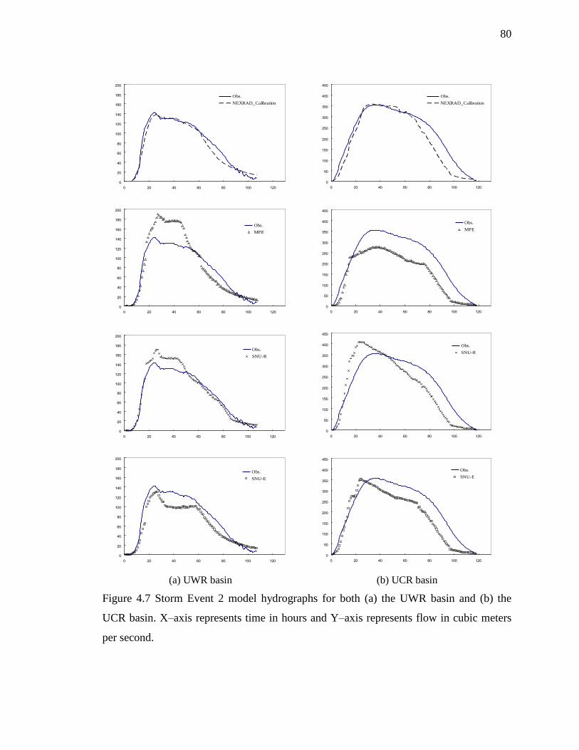
80

0

20

40

60

80

100

120

140

160

180

200

0 20 40 60 80 100 120

Obs.

NEXRAD_Calibration

0

50

100

150

200

250

300

350

400

450

0 20 40 60 80 100 120

Obs.

NEXRAD_Calibration

0

20

40

60

80

100

120

140

160

180

200

0 20 40 60 80 100 120

Obs.

MPE

0

50

100

150

200

250

300

350

400

450

0 20 40 60 80 100 120

Obs.

MPE

0

20

40

60

80

100

120

140

160

180

200

0 20 40 60 80 100 120

Obs.

SNU-R

0

50

100

150

200

250

300

350

400

450

0 20 40 60 80 100 120

Obs.

SNU-R

0

20

40

60

80

100

120

140

160

180

200

0 20 40 60 80 100 120

Obs.

SNU-E

0

50

100

150

200

250

300

350

400

450

0 20 40 60 80 100 120

Obs.

SNU-E




per second.

81

0

50

100

150

200

250

0 20 40 60 80 100 120 140 160 180 200

Obs.

NEXRAD_Calibration

0

50

100

150

200

250

300

350

400

0 20 40 60 80 100 120 140 160 180 200

Obs.

NEXRAD_Calibration

0

50

100

150

200

250

0 20 40 60 80 100 120 140 160 180 200

Obs.

MPE

0

50

100

150

200

250

300

350

400

0 20 40 60 80 100 120 140 160 180 200

Obs.

MPE

0

50

100

150

200

250

0 20 40 60 80 100 120 140 160 180 200

Obs.

SNU-R

0

50

100

150

200

250

300

350

400

0 20 40 60 80 100 120 140 160 180 200

Obs.

SNU-R

0

50

100

150

200

250

0 20 40 60 80 100 120 140 160 180 200

Obs.

SNU-E

0

50

100

150

200

250

300

350

400

0 20 40 60 80 100 120 140 160 180 200

Obs.

SNU-E




per second.

82

0

10

20

30

40

50

60

70

80

90

100

0 50 100 150 200 250

Obs.

NEXRAD_Calibration

0

50

100

150

200

250

300

350

0 50 100 150 200 250

Obs.

NEXRAD_Calibartion

0

10

20

30

40

50

60

70

80

90

100

0 50 100 150 200 250

Obs.

MPE

0

50

100

150

200

250

300

350

0 50 100 150 200 250

Obs.

MPE

0

10

20

30

40

50

60

70

80

90

100

0 50 100 150 200 250

Obs.

SNU-R

0

50

100

150

200

250

300

350

0 50 100 150 200 250

Obs.

SNU-R

0

10

20

30

40

50

60

70

80

90

100

0 50 100 150 200 250

Obs.

SNU-E

0

50

100

150

200

250

300

350

0 50 100 150 200 250

Obs.

SNU-E




per second.

83

0

50

100

150

200

250

0 20 40 60 80 100 120 140 160 180 200

Obs.

NEXRAD_Calibration

0

10

20

30

40

50

60

70

80

90

0 20 40 60 80 100 120 140 160 180 200

Obs.

NEXRAD_Calibration

0

50

100

150

200

250

0 20 40 60 80 100 120 140 160 180 200

Obs.

MPE

0

10

20

30

40

50

60

70

80

90

0 20 40 60 80 100 120 140 160 180 200

Obs.

MPE

0

50

100

150

200

250

0 20 40 60 80 100 120 140 160 180 200

Obs.

SNU-R

0

10

20

30

40

50

60

70

80

90

0 20 40 60 80 100 120 140 160 180 200

Obs.

SNU-R

0

50

100

150

200

250

0 20 40 60 80 100 120 140 160 180 200

Obs.

SNU-E

0

10

20

30

40

50

60

70

80

90

0 20 40 60 80 100 120 140 160 180 200

Obs.

SNU-E




per second.

84

Table 4.8 Details of simulation results with MPE NEXRAD bias corrected rainfall input

for the UWR basin.

Event Simulation with MPE scheme

R2 ENS RMSE(m

3/s) MAPE(%)

1 0.96 0.92 3.51 21.48

2 0.90 0.72 25.83 30.30

3 0.86 0.84 20.43 41.58

4 0.96 0.85 10.63 29.46

5 0.94 0.79 22.08 45.95

Ave. 0.92 0.82 16.49 33.75

Table 4.9 Details of simulation results with SNU–R NEXRAD bias corrected rainfall

input for the UWR basin.

Event Simulation with SNU–R scheme

R2 ENS RMSE(m

3/s) MAPE(%)

1 0.97 0.96 2.56 18.18

2 0.97 0.93 13.13 19.59

3 0.91 0.91 15.54 40.42

4 0.98 0.97 4.94 27.48

5 0.95 0.93 13.12 34.22

Ave. 0.95 0.94 9.86 27.98

85

Table 4.10 Details of simulation results with SNU–E NEXRAD bias corrected rainfall

input for the UWR basin.

Event Simulation with SNU–E scheme

R2 ENS RMSE(m

3/s) MAPE(%)

1 0.97 0.96 2.53 18.19

2 0.96 0.86 18.38 28.24

3 0.91 0.90 16.24 41.26

4 0.97 0.96 5.35 28.63

5 0.94 0.92 13.49 37.66

Ave. 0.95 0.92 11.20 30.80

86

Table 4.11 Details of simulation results with MPE NEXRAD bias corrected rainfall input

for the UCR basin.

Event Simulation with MPE scheme

R2 ENS RMSE(m

3/s) MAPE(%)

1 0.88 0.81 23.24 17.40

2 0.92 0.60 74.64 37.95

3 0.36 0.19 92.02 149.85

4 0.89 0.89 34.51 19.66

5 0.95 0.73 12.40 48.90

Ave. 0.80 0.65 47.36 54.75

Table 4.12 Details of simulation results with SNU–R NEXRAD bias corrected rainfall

input for the UCR basin.

Event Simulation with SNU–R scheme

R2 ENS RMSE(m

3/s) MAPE(%)

1 0.99 0.97 9.42 10.81

2 0.82 0.70 65.16 32.74

3 0.97 0.95 19.48 30.89

4 0.96 0.89 33.74 18.51

5 0.95 0.90 7.59 42.00

Ave. 0.94 0.88 27.08 26.99

87

Table 4.13 Details of simulation results with SNU–E NEXRAD bias corrected rainfall

input for the UCR basin.

Event Simulation with SNU–E scheme

R2 ENS RMSE(m

3/s) MAPE(%)

1 0.96 0.96 11.42 12.69

2 0.89 0.75 59.06 31.22

3 0.97 0.95 18.25 26.69

4 0.94 0.93 27.27 18.76

5 0.94 0.90 7.64 43.42

Ave. 0.94 0.90 24.73 26.56

88

(a)

0

50

100

150

200

250

300

0 50 100 150 200 250 300Observed Peak (cms)

Sim

ula

ted

Pea

k (

cms)

MPE

SNU-R

SNU-E

(b)

0

50

100

150

200

250

300

350

400

450

500

0 50 100 150 200 250 300 350 400 450 500Observed Peak (cms)

Sim

ula

ted

Pea

k (

cms)

MPE

SNU-R

SNU-E

Figure 4.11 Storm events peak discharge (m3/s) scatter plots for (a) the UWR and (b) the

UCR basins.

89

The rainfall input derived by applying spatially uniform bias correction to

NEXRAD data decreased calibrated model prediction accuracy as evident from R2, ENS,

RMSE and MAPE values in comparison to input derived by applying spatially non–

uniform bias correction scheme. The improvement in model results from spatially non–

uniform bias corrected input are better in UCR basin compared to UWR basin because

the NEXRAD values are more variable in time over UCR basin compared to UWR basin

as shown in Fig. 4.4.

Even though the NEXRAD input is adjusted by using gauged rainfall, some under–

prediction or over–prediction of runoff volume and peak flow are found in both study

areas as shown in Figs. 4.6–4.10. Simulations with SNU–E inputs performed the best

with regard to the estimation of peak flow as shown in scatter Fig. 4.11. Similarly, the

input from both methods using spatially non–uniform bias correction produced overall

better output compared to input from spatially uniform bias correction method in terms of

total runoff volume.

4.5. Summary and Conclusions

Three NEXRAD bias corrections are presented in this study. To evaluate the

sensitivity and accuracy of NEXRAD bias corrected rainfall, the Upper Wabash River

and the Upper Cumberland River basins is selected because of different spatial

characteristics. Suggested NEXRAD bias correction schemes are applied to the study

basins to evaluate effects of each NEXRAD bias correction scheme on the variation of

NEXRAD distribution. Simultaneous comparisons of three NEXRAD bias corrected

rainfall are made to cross validate with observed gauge rainfall at down, middle and up

location of two study basins (Fig. 4.1). Improvement in the accuracy of rainfall is

achieved through adjustment of spatially non–uniform NEXRAD bias correction at the

two watersheds in comparison with spatially uniform NEXRAD bias correction. Overall,

spatially non–uniform NEXRAD bias correction performance in comparison to MPE

90

scheme improves from 1.17 to 0.87 mm RMSE in the Upper Wabash River basin, and

from 13.76 to 6.45 mm RMSE in the Upper Cumberland River basin. Spatially non–

uniform NEXRAD bias correction reduces accuracy error in the Upper Wabash River

basin from 41.26% MAPE to 21.37% MAPE, whereas in the Upper Cumberland River

Basin, a large reduction is obtained, 115.35% MAPE to 30.96% MAPE. Use of spatially

non–uniform NEXRAD bias correction in large variability of NEXRAD distribution over

the entire watershed such as the Upper Cumberland River basin is more effective than

small variability of NEXRAD distribution over the entire watershed such as the Upper

Wabash river Basin.

When a spatially uniform bias corrected rainfall input is used in the STORE DHM,

prediction accuracy is degraded. Spatially uniform bias corrected rainfall input produces

inconsistent results with both over prediction and under prediction and no clear trend. To

evaluate sensitivity of rainfall accuracy on hydrologic model simulation, calibrated

parameters in each event are obtained from simulation with original NEXRAD. These

calibrated parameters then are applied to the STORE DHM with three different schemes

of NEXRAD bias corrected rainfall. The accuracy of model prediction with different

NEXRAD bias corrected rainfall is estimated in terms of the R2, ENS, RMSE and MAPE

based on observed data combination. Spatially non–uniform NEXRAD bias corrected

rainfall improves prediction accuracy in both the Upper Wabash River and the Upper

Cumberland River basins. However, a reduction in accuracy of model prediction is

shown in both study areas, when model is used with spatially uniform NEXRAD bias

corrected rainfall. An interpolation scheme that accounts for the spatially non–uniform

NEXRAD bias is applied for reducing spatio–temporal variation of NEXRAD bias. The

spatially non–uniform NEXRAD bias correction proposed in this study uses two different

schemes. Even though these schemes have different procedures before trying the Kalman

filtering, the STORE DHM model simulations with these two NEXRAD bias corrected

rainfall produced nearly equivalent prediction accuracy error statistics and peak flow

error for the events tested that are consistent with both the Upper Wabash River and the

Upper Cumberland River basins.

91

Testing sensitivity to variation of NEXRAD values distribution reveals that the

improvement of prediction accuracy with spatially non–uniform NEXRAD bias corrected

rainfall is greater in larger NEXRAD variation area, whereas, prediction accuracy in

smaller NEXRAD variation area is less improved in comparison to simulation with MPE

scheme rainfall. The large NEXRAD variation at a certain time step implies that each

NEXRAD pixel bias is not uniform, thus NEXRAD bias correction with spatially non–

uniform scheme is much more effective than uniform NEXRAD bias correction scheme.

To evaluate this investigation, this study selects two different characteristics of study

areas: the Upper Wabash River basin has flat terrain with less rainfall variability, and the

Upper Cumberland River basin with relatively mountainous terrain and more variable

rainfall. The results in comparison to simulation with spatially uniform NEXRAD bias

corrected rainfall show that prediction accuracy with spatially non–uniform NEXRAD

bias corrected rainfall in the Upper Cumberland River basin shows more improvement

compared to the Upper Wabash River basin. Consequently, spatially non–uniform

NEXRAD bias correction is an efficient scheme for high NEXRAD variability areas.

92

CHAPTER 5. RESEARCH SYNTHESIS AND FURTURE WORK

5.1. Object–oriented hydrologic model

This research is focused on developing a prototype GIS based tightly coupled

object–oriented framework called GHISMO. The GHISMO has an object–oriented

approach using object–oriented design techniques and object–oriented language, Visual

Basic, to the description and simulation of a watershed based hydrologic process. The

GHISMO allows flexibility and extensibility to investigate future hydrologic issues

without changing its main framework because it uses characteristics of inheritance and

aggregation through an object–oriented hydrologic approach. For example, if object–

oriented based hydrologic models try large scale programming components (infiltration,

Green–Ampt and SCS curve number) at the same time, object–oriented programming can

be easy to manage because each object has a component which has an individual method

and property based on the object class.

Expanding of the GHISMO framework will be essential for robustness of the

hydrologic model. For example, linkage between GHISMO and water quality model (e.g.,

SWAT) can predict effect of storm event on water quality assessment. Similarly, linkage

between the GCMs (General Circulation Models), which are the most advanced tools for

estimating future climate change, and GHISMO will provide a foundation to assess the

impact of climate change on rainfall–runoff prediction. The conceptualization and

characterization of this coupling strategy can be extended to a hydrologic management

and decision supporting tool such as a real–time flood warning system. If the prototype of

the object–oriented hydrologic framework, the GHISMO, is successfully used to develop

a coupled open source and platform for seamless hydrologic components, it may lead to

93

change a hydrologic modeling paradigm to object-oriented approach through its flexible

modeling schemes.

5.2. Parameter Estimation for STORE DHM

Surface roughness has a significant effect on runoff peak flow and time to peak in

rainfall–runoff simulation. Although STORE DHM simulations (the first part of the

broader GHISMO framework) show promising results in comparison with observed

hydrographs, the issue for estimation of surface roughness in different land surface types

is still open to dispute because model calibration only rely on surface roughness for

runoff peak flow and time to peak. For example, surface roughness parameter values at

Fish Creek simulations are out of land use range values (which are provided by Brater

and King (1976)). Also, even though calibrated surface roughness values for each event

are obtained from the same study area (UWR or UCR basin), each calibrated surface

roughness value in the same study shows difference in each land use type.

5.3. Critical Cell Travel Time Criteria

This research suggests CCT to overcome the DEM issue for STORE DHM

simulations. To avoid different simulation results depending on DEM size, this research

uses minimum simulation time step at each event in the particular region. Even though

CCT is theoretically ideal approach for STORE DHM simulation, it still needs to be

refined for physical approach to other hydrologic components and its boundary condition

depending on event types (e.g., small, medium and heavy storm events) and study areas.

94

5.4. Number of Rain gauge for correcting radar bias

Rainfall is a critical factor in hydrologic simulation. However, rainfall varies

substantially in space and time and therefore it is often poorly represented in hydrologic

models. Even though radar rainfall provides a better spatial representation of rainfall

variability, it still suffers from uncertainties and biases. To overcome this limitation, this

research suggests three radar rainfall bias correction schemes (e.g., MPE, SNU–R and

SNU–E). The research results suggest that spatially non–uniform radar bias correction

schemes in large radar variation area are a higher improvement of radar bias correction

over small radar variation area, both in regards to analysis of correcting radar bias and

prediction accuracy of the STORE DHM with different radar bias corrected rainfall.

However, the fundamental issue of minimum number of rain gauge information for

correcting radar bias remains.

95

LIST OF REFERENCES

Adisoma, G.S., and Hester, M.G., 1996. Grade estimation and its precision in mineral

resources: the Jackknife approach. Mining Engineering 48(2), 84–88.

Abbott, M.B., Bathurst, J.C., Cunge, P.E., Rasmussen, J., 1986. An introduction to the

European hydrological system– System hydrologique europeen, “SHE”, 1:

Distributed modeling system. Journal of Hydrology 87, 45–59.

Ajward, M.H., 1996. A spatially distributed unit hydrograph model using a geographic

information system. Ph.D. Dissertation, Civil Engineering Department, University

of Calgary, Calgary.

Anagnostou, E.N., Krajeswski, K.F., Smith, J., 1999. Uncertainty quantification of mean

real radar–rainfall estimates. Journal of Atmospheric and Ocean Technology 16,

206–215

Band, L.E., Tague, C.L., Brun, S.E., Tenenbaum, D.E., Frernandez, R.A., 2000.

Modeling watersheds as spatial object hierarchies: structure and dynamics.

Transaction in GIS 4(3), 181–196.

Beven, K., Moore, I., 1993. Terrain analysis and distributed modeling in hydrology. John

Wiley and Sons: New York.

Beven, K., 2002. Towards an alternative blueprint for a physically based digitally

simulated hydrologic response modeling system. Hydrologic Process 16, 189–206.

Bian, L., Object–oriented representation of environmental phenomena: Is everything best

represented as an object. Annals of the Association of American Geographers 97(2),

267–281.

96

Borga, M., Anagnostou, E.N., Enrico, F., 2000. On the use of real time radar rainfall

estimates for flood prediction in mountainous basins. Journal of Geophysical

Research 105(D2), 2269–2280.

Boyer, J.F., Berkhoff, C., Servat, E., 1996. Object–oriented programming for a

simulation of the rainfall–discharge relationship. In: proceedings of

Hydroinformatics 96. Balkema, A.A. Zurich, Switzerland, pp. 299–305.

Brater, E.F., King, H.W., 1976. Handbook of Hydraulics for the Solution of Hydraulic

Engineering Problems, McGraw–Hill Book Company, New York, USA.

Bronstert, A., Plate, E.J., 1997. Modeling of runoff generation and soil moisture

dynamics for hillslopes and microcatchment. Journal of Hydrology 198, 177–195.

Calver, A., Wood, W.L., 1995, The Institute of Hydrology Distributed Model, In: Shigh,

V.P. (Eds.), Computer Models of Watershed Hydrology, Water resources

Publication, Colorado, pp. 595–626.

Carpenter, T.M., Georgakakos, K.P., Sperfslage, J.A., 2001. On the parametric and

NEXRAD–radar sensitivities of a distributed hydrologic model suitable for

operational use. Journal of Hydrology 254, 169–193.

Chen, H., Beschta, R., 1999. Dynamic hydrologic simulation of the Bear Brook

Wathershed in Maine (BBWM). Environmental Monitoring and Assessment 55,

53–96.

Chow, V.T., Maidment, D.R., Mays, L.W., 1988. Applied Hydrology, McGraw Hill

Publishing, New York, 572 pp.

Ciach, G..j., Krajewski, W.F., 1999. Radar rain gauge comparisons under observational

uncertaintities. Journal of Applied Meteorology 38, 1519–1525.

Desmet, P., Govers G., 1998. Comment on „Modeling topographic potential for erosion

and deposition using GIS‟. International Journal of Geographical Information

Science 10:311–331.

97

Dinku, T., Ananostou, E.N., Borga, M., 2002. Improving radar–based estimation of

rainfall over complex terrain. Journal of Applied Meteorology 41, 1163–1178.

Du, J., Xie, H., Xu, Y., Xu, C., 2009. Development and testing of a new storm runoff

routing approach based on time variant spatially distributed travel time method.

Journal of Hydrology 369, 44–54.

Fairfield, J., Leymarie, P., 1991. Drainage networks from grid digital elevation models.

Water Resources Research 27(5), 709–717.

Famiglietti, J.S., Wood, E.F., 1994. Multiscale modeling of spatially variable water and

energy balance processes. Water Resources Research 30(11), 3061–3078.

Faures, J.M., Goodrich, D.C., Woolhiser, D.A., Sorooshian, S., 1995. Impact of small–

scale rainfall variability on runoff modeling. Journal of hydrology 173, 309–326.

FitzHugh, T.W., Mackay, D.S., 2000. Impacts of input parameter spatial aggregation on

an agricultural nonpoint source pollution model, Journal of Hydrology 236, 35–53.

Fulton, R.A., Breidenbach, J.P., Seo, D., Miller, D.A., O‟Bannon, T., 1998. The WSR–

88D rainfall algorithm. Weather and Forecasting 13, 377–395.

Garrote, L., Becchi, I., 1997. Object–oriented software for distributed rainfall–runoff

models. Journal of Computing in Civil Engineering 11, 190–194.

Goldberg, A. and Rubin, K., 1995. Succeeding with objects. Decision Framework for

Project Management. Addison Wesley Publishing Company, 1995. ISBN 0–201–

62878–3.

Goodchild, M., Parks, B., Steyaert, L., 1993. Environmental Modeling with GIS. Oxford

University Press: Oxford.

Gupta, R.S., 1995. Hydrology and Hydraulic Systems, Waveland Press, 739 pp.

He, C., Croley II, Thomas, E., 2007. Application of a distributed large basin runoff model

in the Great Lakes basin. Control Engineering Practice 15(8), 1001–1011.

98

HEC–GeoRAS user‟s manual available at www.hec.usace.army.mil/software/hec–

ras/hecgeoras.html.

HEC–RAS user‟s manual available at www.hec.usace.army.mil/software/hec–ras/

Johnson, L.E., 1989. MAPHYD–A digital map–based hydrologic modeling system.

Photogrammetric Engineering and Remote Sensing, 55(6), 911–917.

Kang, K., Merwade, V., 2009. Effects of rain gage density on correcting radar

precipitation and its influence on hydrologic model simulation, EOS Transactions

AGU, 90(52), Fall meeting, San Francisco, CA, December 2009.

Kiker, G.A., Clark, D.J., Martinez, C.J., Schulz, R.E., 2006. A java based, object–

oriented modeling system for southern African hydrology. Transactions of ASABE

49 (5), 1419–1433.

Kilgore, R.T., Krolak, J.S., Walsh, M., 1994. Integration of water resource models and

GIS for water resource management. Water Policy and Management: Solving the

Problems; Process, Conference, ASCE, New York, 37–40.

Koren, V., Smith, M., Duan, Q., 2003. Use of a priori parameter estimates in the

derivation of spatially consistent parameter sets of rainfall–runoff models. In: Daun,

Q., Sorooshian, S., Gupta, H., Rosseau, A., Turotte, R. (Eds.), Calibration of

Watershed Models, AGU Water Science and Applications Series.

Kralisch, S., Krause, P., David, O., 2005. Using the object modeling system for

hydrological model development and application. Advances in Geosciences 4, 75–

81.

Lahlou, M., Shoemaker, L., Choudry, S., Elmer, R., Hu, A., Manguerra, H., Parker, A.,

1998. Better assessment science integration point and nonpoint sources: BASIN 2.0

User‟s Manual. EPA–823–B–98–006, U.S. Environmental Protection Agency,

Office of Water, Washington, DC, USA.

Lal, A.M.W., Van Zee, R., Belnap, M., 2005. Case study: model to simulate regional

flow in South Florida. Journal of Hydraulic Engineering 131(4), 247–258.

99

Legates, D.R., 2000. Real–time calibration of radar precipitation estimates. Professional

Geographer 52(2), 235–246.

Leipnick, M.R., Kemp, K.K., Loaiciga, H.A., 1993. Implementation of GIS for water

resources planning and management. Journal of Water Resource Planning and

Management 119(2), 184–205.

Li, M., Shao, Q., 2010. An improved statistical approach to merge satellite rainfall

estimates and raingauge data. Journal of Hydrology, In press.

Liu, Y.B., Gebremeskel, S., Smedt, F., Hoffmann, L., Pfister, L., 2003. A diffusive

transport approach for flow routing in GIS–based flood modeling. Journal of

Hydrology 283(1–4), 91–106.

Looper, J., Vieux, B., Moreno, M., 2009. Assessing the impacts of precipitation bias on

distributed hydrologic model calibration and prediction accuracy. Journal of

Hydrology, In press.

Loucks, D.P., Kindler, J. and Fedra, K., 1985. Interactive water resources modeling and

model use: An overview. Water Resources Research, 21(2), 95–102.

Luzio, Di, M., Srinivasan, R., Arnodl, J. G., Neitsch, S. L., 2002. Arcview Interface for

SWAT2000. User‟s Guide. U.S. Department of Agriculture, Agriculture Research

Service. Temple, Texas.

Maidment, D.R., 1993. GIS and hydrologic modeling. In: Goodchild, M., Parks, B.,

Steyaert, L. (Eds.), Environmental Modeling With GIS. Oxford University Press,

New York, USA.

Maidment, D.R., Olivera, J.F., Calver, A., Eatherall, A., Fraczek, W., 1996. A unit

hydrograph derived from a spatially distributed velocity field. Hydrologic

Processes 10, 831–844.

Maidment, D.R., 2002. ArcHydro GIS for Water Resources, ESRI Press, California, 203

pp.

100

Madsen, H., 2003. Parameter estimation in distributed hydrological catchment modeling

using automatic calibration with multiple objectives. Advances in Water resources

26(2), 205–216.

McKim, H.L., Cassell, E.A., Lapotin, P.J., 1993. Water resource modelling using remote

sensing and object–oriented simulation. Hydrological Processes 7, 153–165.

Melesse, A.M., 2002. Spatially distributed storm runoff modeling using remote sensing

and geographic information system. Ph. D. Dissertation, University of Florida.

Melesse, A.M., Graham, W.D., 2004. Storm runoff prediction based on a spatially

distributed travel time method utilizing remote sensing and GIS. Journal of the

American Water Resources Association 40(4), 863–879.

Molnar, D.K., Julien, P.Y., 2000. Grid–size effects on surface runoff modeling. Journal

of Hydrol. Eng. ASCE 5 (1), 8–16.

Montgomery, D., Dietrich, W., 1994. A physically based model for the topographic

control on shallow landsliding. Water Resources Research 30, 1153–1171.

Moore, I., Grayson, R., Ladson, A., 1991. Digital terrain modeling: a review of

hydrological, geomorphological and biological applications. Hydrologic Processes

5, 3–30.

Moreda, F., Koren, V., Zhang, Z., Reed, S., Smith M., 2006. Parameterization of

distributed hydrological models: learning from the experiences of lumped

modeling. Journal of Hydrology 320(1–2), 218–237.

Muzic, I., 1995. GIS derived distributed unit hydrograph, a new tool for flood modeling.

In: Topping, B. (Ed.), Developments in Computer Aided Design and Modeling for

Civil Engineering. Civil–Component Press, Edinburgh, UK, pp. 243–247.

Muzic, I. 1996. Lumped modeling and GIS in flood prediction. Geographical Information

Systems in Hydorlogy, Kluwer Academic Publishers.

Nash, J.E., and J.V. Sutcliffe. 1970. River flow forecasting through conceptual models:

Part 1. A discussion of principles. Journal of Hydrology 10(3), 282–290.

101

Nelson, E. J., 1997. WMS v5.0 Reference Manual, Environmental Modeling Research

Laboratory, Brigham Young University, Provo, Utah.

Nelson, E. J., Jones, N. L., and Jorgeson, J. D., 1995. A comprehensive environment for

watershed modling and hydrologic analysis. Process, Conference, ASCE, New

York, 897–901.

Nuss, W.A. and Titley, D.W., 1990. Use of multiquadric interpolation for meteorological

objective analysis. Monthly Weather Review 122, 1611–1631.

O‟Callaghan, J.F., Mark, D.M., 1984. The extraction of drainage networks from digital

elevation data. Computer Vision, Graphics and Image Processing 28, 324–344.

Ogden, F.L., garbrecht, J., DeBarry, P.A., Johnson, L.E., 2001. GIS and distributed

watershed models, II: Modules, interfaces and models. Journal of Hydrologic

Engineering 6(6), 515–523.

Olivera, F., Maidment, D., 1999. Geographic Information System (GIS)–based spatially

distributed model for runoff routing. Water Resources Research 35(4), 1155–1164.

O‟Loughlin, E., 1986. Prediction of surface saturation zones in natural catchments by

topographic analysis. Water Resources Research 22: 794–804.

Peucker, T.K., Douglas, D.H., 1975. Detection of surface specific points by local parallel

processing of discrete terrain elevation data. Computer graphics and Image

Processing 4, 375–387.

Ponce, V.M., Engineering Hydrology. Prince–Hall, New Jersey, 640p.

Reed, S.M., Maidment, D.R., 1995. A GIS procedure for merging NEXRAD

precipitation data and digital elevation models to determine rainfall–runoff

modeling parameters. Center for Research in Water Resources (CRWR),

University of Texas at Austin Online Report 95–3, pp. 119.

Reed, S.M., Maidment, D.R., 1999. Coordinate transformations for using NEXRAD data

in GIS–based hydrologic modeling, Journal of Hydrologic Engineering 4, 174–182.

102

Refsgaard, J., 1997. Parameterization, calibration and validation of distributed

hydrological models. Journal of Hydrology 198 (1–4), 69–97.

Reitsma, R. F., Sautins, A. M., and Wehrend, S. C., 1994. Construction kit for visual

programming of river–basin models. Journal of Computing in Civil Engineering

8(3), 378–384.

Remesan, R., Shamim, M., 2009. Runoff prediction using an integrated hybrid modeling

scheme. Journal of Hydrology 372, 48–60.

Richardson, M.C., Branfireun, B.A., Robinson, V.B., Graniero, P.A., 2007. Towards

simulating biogeochemical hot spots in the landscape: A geographic object–based

approach. Journal of Hydrology 342(1–2), 97–109.

Ripley, D.B., 1981. Spatial Statistics. Wiley, New York, USA. 252pp.

Seo, D.J., Breidenbach, J.P., Johnson, E.R., 1999. Real–time estimation of mean field

bias in radar rainfall data. Journal of Hydrology 223, 131–147.

Seo, D.J., Breidenbach, J.P., 2002. Real–time correction of spatially nonuniform bias in

radar rainfall data using rain gauge measurements. Journal of Hydrometeorology 2,

93–111.

Shedd, R.C., Fulton, R.A., 1993. WRS–88D precipitation processing and its use in

National Weather Service hydrologic forecasting. Proceeding of ASCE

Internationa Symposiumon Engineering Hydrology.

Sherman, L.K., 1932. Streamflow from rainfall by unit graph method. Engineering News

Record 108, 501–505.

Simanton, J.R. and Osborn, H.B., 1980. Reciprocal distance estimate of point rainfall.

Journal of the Hydraulics Division, ASCE 106, 1242–1246.

Singh, V.P., Aravamuthan, V., 1996. Errors of kinematic–wave and diffusion–wave

approximations for steady–state overland flows. Catena 27, 209–227.

103

Smith, C.J., 1986. The reduction of errors caused by bright bands in quantitative rainfall

measurements made using radar. Journal of Atmospheric and Oceanic Technology

3, 129–141.

Smith, J.A., Krajeswski, 1991. Estimation of the mean field bias of radar rainfall

estimates. Journal of applied Meteorology 30, 397–412.

Smith, J.A., Seo, D.J., Baeck, M.L., Hudlow, M.D., 1996. An intercomparison study of

NEXRAD precipitation estimates. Water Resources Research 31, 2035–2045.

Smith, M.B., Seo, D. J., Koren, Ⅴ.Ⅰ., et al., 2004. The distributed model intercomparison

project (DMIP); an overview. Journal of Hydrology 298(1–4), 4–26.

Stellman, K.M., Fuelberg, H.E., Garza, R., Mullusky, M., 2001. An estimation of radar

and rain gauge–derived mean areal precipitation over Georgia watersheds. Weather

Forecast 16, 133–144.

Tarboton, D.G., 1997. A new method for the determination of flow directions and

upslope areas in grid digital elevation models. Water Resources Research 32, 309–

319.

Thieken, A.H., Lucke, A., 1999. Scaling input data by GIS for hydrological modeling.

Hydrologic Process 13(4), 611–630.

Troutman, B.M., Karlinger, M.R., Guerin, D.P., 1989. Basin–scale relations via

conditioning. Stochastic Hydrology and Hydraulics 3, 111–133.

U.S Army Corps of Engineers (USACE), 1998. HEC–HMS hydrologic modeling system

user‟s manual–version 1.0. Hydrologic Engineering Center, Davis, California.

Vazquez, R.F., Feyen, L., 2004. Potential evapotranspiration for the distributed modeling

of Belgian basins. Journal of Irrigation and Drainage Engineering 130(1), 1–8.

Vertessey, R.A., Hatton, T.J., O‟Shaughnessy, Jayasuriya, M.D.A., 1993. Predicting

water yield from a mountain ash forest catchment using a terrain analysis based

catchment model. Journal of Hydrology 150, 665–700.

104

Wang, J., Hassett, J.M., Endreny, T.A., 2005. An object oriented approach to the

description and simulation of watershed scale hydrologic processes, Computers and

Geosciences 31(4), 425–435.

Ware, E.C., 2005. Correction to radar–estimated precipitation using observed rain gauge

data. MS thesis, Cornell University, Ithaca, 87.

Welch, G., Bishop, G., 2001. An Introduction to the Kalman Filter. SIGGRAPH 2001

course 8. In Computer Graphics, Annual Conference Graphics & Interactive

Techniques. ACM Press.

Wilson, J.W., Brandes, E., 1979. Radar measurement of rainfall– A summary. American

Meteorology Society 60, 1048–1058.

Wilson, J.P., gallant, J.C., 2000. Terrain Analysis: Principles and Applications. John

Wiley and Sons: New York.

Winchell, M., Gupta, H.V., Sorooshian, S., 1998. On the simulation of infiltration and

saturation excess runoff using radar–based rainfall estimates: Effects of algorithm

uncertainty and pixel aggregation. Water Resources Research 34(10), 2655–2670.

Wise, S., 2000. Assessing the quality for hydrological applications of digital elevation

models derived from contours. Hydrological Processes 14: 1909–1929.

Xie, H., Zhou, X., 2005. GIS–based NEXRAD Stage III precipitation database:

automated approaches for data processing and visualization, Computers and

Geosciences 31, 65–76.

Xie, H., Zhou, X., Hendricks, J., Vivoni, E., Guan, H., Tian, Y., Small, E., 2006.

Evaluation of NEXRAD Stage III precipitation data over semiarid region. Journal

of the American Water Resources Association 42(1), 237–256.

Young, C.B., Bradley, A.A., Krajewski, W.F., Kruger, A., Morrissey, M.L., 2000.

Evaluating NEXRAD multisensor precipitation estimates for operational

hydrologic forecasting. Journal of Applied Meteorology 14, 1430–1436.

105

Zhang, W., Montgomery, D.R., 1994. Digital elevation model grid size, landscape representation,

and hydrologic simulations. Water Resources Research 30(4), 1019–1028.

106

Appendix A.

Local Bias Correction Procedure Used in Process 1 (P1)

In the simplest terms, the local bias correction procedure used in P1 may be

described by the following:

3 3

0

1 1

c i i i i

i i

r r w w Eq. A.1

where

1 if /

/ if /

i i i

i

i i i i i

g r

g r g r

Eq. A.2

if /

0 if /

i i i i i

i

i i i

g r g r

g r.

Eq. A.3

In Eq. A.1, rc denotes the bias–corrected radar rainfall (mm), r0 denotes the raw radar

rainfall at the bin centered at u0 (mm), wi denotes the weight given to the radar–gauge pair

at the ith

vertex in the triangle of radar–gauge pairs that encloses u0, i

denotes the

multiplicative sample bias from the ith radar–gauge pair, and i

denotes the additive

sample bias from the ith radar–gauge pair. In Eqs. A.2 and A.3, ig and

ir denote the

gauge rainfall measurement (mm) and the collocation radar rainfall estimate (mm),

respectively, at the ith

vertex in the enclosing triangle, and i , an adaptable parameter,

denotes the threshold for the multiplicative sample bias, /i ig r , i = 1,2,3. The neighboring

107

radar–gauge pairs are identified by “triangulation,” which connects all available radar–

gauge pairs into a mesh of triangles. The weights, wi, i = 1,2,3, sum to unity and are

inversely proportional to the distance to the neighboring radar–gauge pairs in the

enclosing triangle.

108

Appendix B.

Exponential Smoothing of Bin–Averaged Gauge Rainfall Using Gauge Measurements

The observation equation for the bin–average gauge rainfall centered at u0 at hour k,

G0k, is given by

0 Vgk k k gkG Eq. B.1

where the observation vector Zgk; the structure vector Hk; the unknown bin–averaged

gauge rainfall centered at u0, G0k; and the error vector Vgk; are given by [g1k, g2k, g3k, g4k,

g5k, g6k, ……, g(nk)k]T; [1, 1, 1, 1, 1, 1, 1, 1, 1, 1, ……, 1]T; 1

00

( )kA

A P u du ; and

T1 1 1

1 0 2 0 00 0 0

( ) , ( ) ,..., ( )k k k k nk kA A A

G A P u du G A P u du G A P u du , respectively.

In the above, gik denotes the ith

rain gauge measurement at hour k, and P(u) denotes the

point hourly gauge rainfall at location u within the bin. The ijth

entry in the error

covariance matrix of Vgk, gk, is then given by

1 1

0 00 0

cov ( ) , ( )gijk ik k jk kA A

G A P u du G A P u du

Eq. B.2a

2

00 0

cov ( ), ( )gijk k kA A

A P u P v dudv

1

00cov , ( )ik k

AA G P u du

1

00cov ( ), cov ,k jk ik jk

AA P u G du G G

Eq. B.2b

109

1

00

, ( )gijk ik kA

A G P u du

1

00

( ),k jkA

A P u G du

2

00 0

( ), ( ) , ,k k ik jkA A

A P u P v dudv G G

Eq. B.2c

where cov[] and [] denote the covariance and the semivariogram, respectively.

110

Appendix C.

Effect of Using Gauge Measurements, in lieu of Areally Averaged Gauge Rainfall, on

Mean Square Error Calculations

The mean square error of raw radar–gauge estimates with respect to the gauge

measurements, mse[Rr – P(u)] is an estimate of E{[Rr – P(u)]2}, where Rr denotes the raw

radar rainfall and P(u) denotes the gauge rainfall at some point u within the radar bin. We

may rewrite E{[Rr – P(u)]2} as

2 2{[ ( )] } {[ ( )] }.r rE R P u E R G G P u Eq. C.1

In the avove, G denotes the areally averaged gauge rainfall over the radar bin, that is,

1

00

( )A

G A P u du , where A0 denotes the area of the bin. Then, under the assumption

that the estimation error in the raw radar rainfall estimate, Rr – G, and the sampling error

in the gauge measurement due to microscale variability of rainfall, G – P(u), are linearly

independent (Drake 1967; Ciach and Krajewski 1999 for justification), we may write

2 2{[ ( )] } [( ) ] var[ ( )].r rE R P u E R G G P u Eq. C.2

Likewise, under the similar assumption that Rc – G and G – P(u) are linearly independent,

where Rc denotes the bias corrected radar rainfall, we may write

2 2{[ ( )] } [( ) ] var[ ( )].c cE R P u E R G G P u Eq. C.3

From Eqs. D.2 and D.3, we then have

111

2 2 2 2{[ ( )] } {[ ( )] } [( ) ] [( ) ]r c r cE R P u E R P u E R G E R G Eq. C.4

2 2 2 2

2 2

{[ ( )] } {[ ( )] } [( ) ] [( ) ]

{[ ( )] } [( ) ]

r c r c

r r

E R P u E R P u E R G E R G

E R P u E R G

Eq. C.5

In other words, the true reduction in mean square error based on bin–averaged gauge

rainfall, mse[Rr – G] – mse[Rc – G], is approximately the same as the apparent reduction,

mse[Rr – P(u)] – mse[Rc – P(u)], based on rain gauge measurements, and the true percent

reduction in mean square error based on bin–averaged gauge rainfall is larger than the

apparent percent reduction based on rain gauge measurements.

112

VITA

Kwangmin Kang was born in Masan, South Korea. He received his Bachelor of

Engineering degree from Kyonggi University, South Korea, and Master of Science

degree from University of Florida, United States. He joined the Ph.D. program of Purdue

University in August 2007.

LIST OF REFERENCES

APPENDICES

object oriented hydrologic modeling with gis …vmerwade/reports/2011_02.pdf · object–oriented...

Documents