oases version 3.1 user guide and reference manualoceanai.mit.edu/lamss/docs/oases_manual.pdf ·...
TRANSCRIPT

OASESVersion 3.1
User Guide and Reference Manual
Henrik SchmidtDepartment of Ocean Engineering
Massachusetts Institute of Technology
March 11, 2011
1

CONTENTS 2
Contents
1 Introduction 10
2 Installing OASES 11
2.1 Loading OASES files . . . . . . . . . . . . . . . . . . . . . . . . . . . . . . . 11
2.2 Building OASES Package . . . . . . . . . . . . . . . . . . . . . . . . . . . .12
2.2.1 Compiler Definitions . . . . . . . . . . . . . . . . . . . . . . . . . . . 13
2.2.2 Parameter settings . . . . . . . . . . . . . . . . . . . . . . . . . . . . 14
2.3 Building PLOTMTV . . . . . . . . . . . . . . . . . . . . . . . . . . . . . . . 15
3 System Settings 16
3.1 Executable Path . . . . . . . . . . . . . . . . . . . . . . . . . . . . . . . . . .16
3.2 Environmental Parameters . . . . . . . . . . . . . . . . . . . . . . . . .. . . 16
4 OASES - General Features 18
4.1 Environmental Models . . . . . . . . . . . . . . . . . . . . . . . . . . . . .. 18
4.1.1 Transversily Isotropic Media . . . . . . . . . . . . . . . . . . . .. . . 18
4.1.2 Dispersive Media . . . . . . . . . . . . . . . . . . . . . . . . . . . . . 19
4.1.3 Porous Media . . . . . . . . . . . . . . . . . . . . . . . . . . . . . . . 20
4.1.4 Continuous Sound Speed Profiles . . . . . . . . . . . . . . . . . . .. 22
4.1.5 Stratified Fluid Flow . . . . . . . . . . . . . . . . . . . . . . . . . . . 23
5 OASR: OASES Reflection Coefficient Module 24
5.1 Input Files for OASR . . . . . . . . . . . . . . . . . . . . . . . . . . . . . . .24
5.1.1 Block I: Title . . . . . . . . . . . . . . . . . . . . . . . . . . . . . . . 24
5.1.2 Block II: OASR options . . . . . . . . . . . . . . . . . . . . . . . . . 24
5.1.3 Block IV: Environmental Model . . . . . . . . . . . . . . . . . . . .. 27
CONTENTS 3
5.2 Execution of OASR . . . . . . . . . . . . . . . . . . . . . . . . . . . . . . . . 28
5.3 Graphics . . . . . . . . . . . . . . . . . . . . . . . . . . . . . . . . . . . . . . 28
5.4 Output Files . . . . . . . . . . . . . . . . . . . . . . . . . . . . . . . . . . . . 29
5.5 OASR - Examples . . . . . . . . . . . . . . . . . . . . . . . . . . . . . . . . . 30
6 OAST: OASES Transmission Loss Module 33
6.1 Input Files for OAST . . . . . . . . . . . . . . . . . . . . . . . . . . . . . . .33
6.1.1 Block I: Title . . . . . . . . . . . . . . . . . . . . . . . . . . . . . . . 33
6.1.2 Block II: OAST options . . . . . . . . . . . . . . . . . . . . . . . . . 33
6.1.3 Block III: Frequencies . . . . . . . . . . . . . . . . . . . . . . . . . .38
6.1.4 Block IV: Environmental Model . . . . . . . . . . . . . . . . . . . .. 38
6.1.5 Block V: Sources . . . . . . . . . . . . . . . . . . . . . . . . . . . . . 39
6.1.6 Block VI: Receivers . . . . . . . . . . . . . . . . . . . . . . . . . . . 41
6.1.7 Block VII: Wavenumber Integration . . . . . . . . . . . . . . . .. . . 42
6.2 Execution of OAST . . . . . . . . . . . . . . . . . . . . . . . . . . . . . . . . 43
6.3 Graphics . . . . . . . . . . . . . . . . . . . . . . . . . . . . . . . . . . . . . . 44
7 RDOAST: OASES Range-dependent TL Module 45
7.1 Input Files for RDOAST . . . . . . . . . . . . . . . . . . . . . . . . . . . . .45
7.1.1 Block I: Title . . . . . . . . . . . . . . . . . . . . . . . . . . . . . . . 45
7.1.2 Block II: RDOAST options . . . . . . . . . . . . . . . . . . . . . . . . 45
7.1.3 Block III: Frequencies . . . . . . . . . . . . . . . . . . . . . . . . . .50
7.1.4 Block IV: Environmental Model . . . . . . . . . . . . . . . . . . . .. 51
7.1.5 Block V: Sources . . . . . . . . . . . . . . . . . . . . . . . . . . . . . 51
7.1.6 Block VI: Receivers . . . . . . . . . . . . . . . . . . . . . . . . . . . 53
7.1.7 Block VII: Wavenumber Integration . . . . . . . . . . . . . . . .. . . 54
7.2 Execution of RDOAST . . . . . . . . . . . . . . . . . . . . . . . . . . . . . . 55

CONTENTS 4
7.3 Graphics . . . . . . . . . . . . . . . . . . . . . . . . . . . . . . . . . . . . . . 55
7.4 RDOAST - Examples . . . . . . . . . . . . . . . . . . . . . . . . . . . . . . . 56
7.4.1 Reverberation Benchmark problem . . . . . . . . . . . . . . . . .. . 56
8 OASP: 2-D Wideband Transfer Functions 59
8.1 Two-Step Execution . . . . . . . . . . . . . . . . . . . . . . . . . . . . . . .. 59
8.2 Transfer Functions . . . . . . . . . . . . . . . . . . . . . . . . . . . . . . .. 59
8.3 Input Files for OASP . . . . . . . . . . . . . . . . . . . . . . . . . . . . . . .60
8.4 Block I: Title . . . . . . . . . . . . . . . . . . . . . . . . . . . . . . . . . . . 60
8.5 Block II: OASP options . . . . . . . . . . . . . . . . . . . . . . . . . . . . .. 60
8.5.1 Block III: Source Frequency . . . . . . . . . . . . . . . . . . . . . .. 64
8.5.2 Block IV: Environmental Model . . . . . . . . . . . . . . . . . . . .. 64
8.5.3 Block V: Sources . . . . . . . . . . . . . . . . . . . . . . . . . . . . . 65
8.5.4 Block VI: Receivers . . . . . . . . . . . . . . . . . . . . . . . . . . . 68
8.5.5 Block VII: Wavenumber integration . . . . . . . . . . . . . . . .. . . 70
8.6 Execution of OASP . . . . . . . . . . . . . . . . . . . . . . . . . . . . . . . . 71
8.7 Graphics . . . . . . . . . . . . . . . . . . . . . . . . . . . . . . . . . . . . . . 72
8.8 OASP - Examples . . . . . . . . . . . . . . . . . . . . . . . . . . . . . . . . . 73
8.8.1 OASP Transmission loss calculation . . . . . . . . . . . . . . .. . . . 73
9 RDOASP: 2-D Range-dependent Transfer Functions 75
9.1 Transfer Functions . . . . . . . . . . . . . . . . . . . . . . . . . . . . . . .. 75
9.2 Input Files for RDOASP . . . . . . . . . . . . . . . . . . . . . . . . . . . . .75
9.3 Block I: Title . . . . . . . . . . . . . . . . . . . . . . . . . . . . . . . . . . . 75
9.4 Block II: RDOASP options . . . . . . . . . . . . . . . . . . . . . . . . . . .. 77
9.4.1 Block III: Source Frequency . . . . . . . . . . . . . . . . . . . . . .. 79
9.4.2 Block IV: Environmental Model . . . . . . . . . . . . . . . . . . . .. 80

CONTENTS 5
9.4.3 Block V: Sources . . . . . . . . . . . . . . . . . . . . . . . . . . . . . 81
9.4.4 Block VI: Receivers . . . . . . . . . . . . . . . . . . . . . . . . . . . 81
9.4.5 Block VII: Wavenumber integration . . . . . . . . . . . . . . . .. . . 82
9.5 Execution of RDOASP . . . . . . . . . . . . . . . . . . . . . . . . . . . . . . 83
9.6 Graphics . . . . . . . . . . . . . . . . . . . . . . . . . . . . . . . . . . . . . . 83
10 OASP3D: 3-D Wideband Transfer Functions 85
10.1 Two-Step Execution . . . . . . . . . . . . . . . . . . . . . . . . . . . . . .. . 85
10.2 OASP3D Options . . . . . . . . . . . . . . . . . . . . . . . . . . . . . . . . . 85
10.3 Sources . . . . . . . . . . . . . . . . . . . . . . . . . . . . . . . . . . . . . . 86
10.3.1 Source Types . . . . . . . . . . . . . . . . . . . . . . . . . . . . . . . 87
10.3.2 User defined Source Arrays . . . . . . . . . . . . . . . . . . . . . . .88
10.4 Receivers . . . . . . . . . . . . . . . . . . . . . . . . . . . . . . . . . . . . . 90
10.4.1 Non-equidistant Receiver Depths . . . . . . . . . . . . . . . .. . . . 91
10.4.2 Tilted Receiver Arrays . . . . . . . . . . . . . . . . . . . . . . . . .. 91
10.5 Execution of OASP3D . . . . . . . . . . . . . . . . . . . . . . . . . . . . . .92
10.6 Graphics . . . . . . . . . . . . . . . . . . . . . . . . . . . . . . . . . . . . . . 92
11 OASN: Noise, Covariance Matrices and Signal Replicas 93
11.1 Input Files for OASN . . . . . . . . . . . . . . . . . . . . . . . . . . . . . .. 93
11.1.1 Block I: Title of Run . . . . . . . . . . . . . . . . . . . . . . . . . . . 93
11.1.2 Block II: Computational options . . . . . . . . . . . . . . . . .. . . . 93
11.1.3 Block III: Frequency Selection . . . . . . . . . . . . . . . . . .. . . . 97
11.1.4 Block IV: Environmental Data . . . . . . . . . . . . . . . . . . . .. . 97
11.1.5 Block V: Receiver Array . . . . . . . . . . . . . . . . . . . . . . . . .97
11.1.6 Block VI: Noise and Signal Sources . . . . . . . . . . . . . . . .. . . 98
11.1.7 Block VII: Surface Noise Parameters . . . . . . . . . . . . . .. . . . 98

CONTENTS 6
11.1.8 Block VIII: Deep Noise Source Parameters . . . . . . . . . .. . . . . 99
11.1.9 Block IX: Discrete Noise and Signal Sources . . . . . . . .. . . . . . 99
11.1.10 Block X: Signal Replica Parameters . . . . . . . . . . . . . .. . . . . 100
11.1.11 Source Level Input Files . . . . . . . . . . . . . . . . . . . . . . .. . 100
11.1.12 Examples . . . . . . . . . . . . . . . . . . . . . . . . . . . . . . . . . 101
11.2 Execution of OASN . . . . . . . . . . . . . . . . . . . . . . . . . . . . . . . .102
11.3 Graphics . . . . . . . . . . . . . . . . . . . . . . . . . . . . . . . . . . . . . . 103
11.4 Output Files . . . . . . . . . . . . . . . . . . . . . . . . . . . . . . . . . . . .103
11.4.1 Covariance Matrices . . . . . . . . . . . . . . . . . . . . . . . . . . .103
11.4.2 Replica Fields . . . . . . . . . . . . . . . . . . . . . . . . . . . . . . 105
12 OASI: Environmental Inversion 107
12.1 Input Files for OASI . . . . . . . . . . . . . . . . . . . . . . . . . . . . . .. 107
12.1.1 Block I: Title of Run . . . . . . . . . . . . . . . . . . . . . . . . . . . 107
12.1.2 Block II: Computational options . . . . . . . . . . . . . . . . .. . . . 107
12.1.3 Block III: Frequency Selection . . . . . . . . . . . . . . . . . .. . . . 111
12.1.4 Block IV: Environmental Data . . . . . . . . . . . . . . . . . . . .. . 111
12.1.5 Block V: Receiver Array . . . . . . . . . . . . . . . . . . . . . . . . .111
12.1.6 Block VI: Noise and Signal Sources . . . . . . . . . . . . . . . .. . . 112
12.1.7 Block VII: Surface Noise Parameters . . . . . . . . . . . . . .. . . . 112
12.1.8 Block VIII: Deep Noise Source Parameters . . . . . . . . . .. . . . . 113
12.1.9 Block IX: Discrete Noise and Signal Sources . . . . . . . .. . . . . . 113
12.1.10 Block X: Signal Replica Parameters . . . . . . . . . . . . . .. . . . . 114
12.1.11 Examples . . . . . . . . . . . . . . . . . . . . . . . . . . . . . . . . . 114
12.2 Execution of OASI . . . . . . . . . . . . . . . . . . . . . . . . . . . . . . . .115
12.3 Graphics . . . . . . . . . . . . . . . . . . . . . . . . . . . . . . . . . . . . . . 116
CONTENTS 7
12.4 Output Files . . . . . . . . . . . . . . . . . . . . . . . . . . . . . . . . . . . .116
13 OASM: Matched Field Processing Module 117
13.1 Input Files for OASM . . . . . . . . . . . . . . . . . . . . . . . . . . . . . .. 117
13.1.1 Block I: Title of Run . . . . . . . . . . . . . . . . . . . . . . . . . . . 117
13.1.2 Block II: Computational options . . . . . . . . . . . . . . . . .. . . . 117
13.1.3 Block III: Frequency Selection . . . . . . . . . . . . . . . . . .. . . . 119
13.1.4 Block V: Receiver Array . . . . . . . . . . . . . . . . . . . . . . . . .119
13.1.5 Block V: Signal Replica Parameters . . . . . . . . . . . . . . .. . . . 120
13.1.6 Block VI: Reference Sound Speed . . . . . . . . . . . . . . . . . .. . 120
13.1.7 Block VII: Tolerant Beamformer . . . . . . . . . . . . . . . . . .. . . 120
13.1.8 Block VIII: Signal Blurring . . . . . . . . . . . . . . . . . . . . .. . 121
13.1.9 Examples . . . . . . . . . . . . . . . . . . . . . . . . . . . . . . . . . 121
13.2 Execution of OASM . . . . . . . . . . . . . . . . . . . . . . . . . . . . . . . 122
13.3 Graphics . . . . . . . . . . . . . . . . . . . . . . . . . . . . . . . . . . . . . . 122
14 OASS: OASES Scattering and Reverberation Module 124
14.1 Input Files for OASS . . . . . . . . . . . . . . . . . . . . . . . . . . . . . .. 124
14.1.1 Block I: Title of Run . . . . . . . . . . . . . . . . . . . . . . . . . . . 124
14.1.2 Block II: Computational options . . . . . . . . . . . . . . . . .. . . . 126
14.1.3 Block III: Frequency Selection . . . . . . . . . . . . . . . . . .. . . . 127
14.1.4 Block IV: Environmental Data . . . . . . . . . . . . . . . . . . . .. . 127
14.1.5 Block V: Scattering parameters . . . . . . . . . . . . . . . . . .. . . 127
14.1.6 Block VI: Receiver Array . . . . . . . . . . . . . . . . . . . . . . . .127
14.1.7 Block VII: Wavenumber Sampling . . . . . . . . . . . . . . . . . .. . 128
14.1.8 Block VIII: Range Offsets . . . . . . . . . . . . . . . . . . . . . . .. 128
14.1.9 Block VIII: Range Increments . . . . . . . . . . . . . . . . . . . .. . 128

CONTENTS 8
14.1.10 Examples . . . . . . . . . . . . . . . . . . . . . . . . . . . . . . . . . 129
14.2 Execution of OASS . . . . . . . . . . . . . . . . . . . . . . . . . . . . . . . .132
14.3 Graphics . . . . . . . . . . . . . . . . . . . . . . . . . . . . . . . . . . . . . . 132
14.4 Output Files . . . . . . . . . . . . . . . . . . . . . . . . . . . . . . . . . . . .132
14.4.1 Covariance Matrices . . . . . . . . . . . . . . . . . . . . . . . . . . .133
15 OASSP: 2-D Waveguide Reverberation Realizations 135
15.1 Transfer Functions . . . . . . . . . . . . . . . . . . . . . . . . . . . . . .. . 135
15.2 Input Files for OASSP . . . . . . . . . . . . . . . . . . . . . . . . . . . . .. 135
15.3 Block I: Title . . . . . . . . . . . . . . . . . . . . . . . . . . . . . . . . . . .135
15.4 Block II: OASSP options . . . . . . . . . . . . . . . . . . . . . . . . . . .. . 137
15.4.1 Block III: Source Frequency . . . . . . . . . . . . . . . . . . . . .. . 139
15.4.2 Block IV: Environmental Model . . . . . . . . . . . . . . . . . . .. . 140
15.4.3 Volume Scattering Layer . . . . . . . . . . . . . . . . . . . . . . . .. 141
15.4.4 Block V: Sources . . . . . . . . . . . . . . . . . . . . . . . . . . . . . 141
15.4.5 Block VI: Receivers . . . . . . . . . . . . . . . . . . . . . . . . . . . 142
15.4.6 Block VII: Wavenumber integration . . . . . . . . . . . . . . .. . . . 143
15.5 Execution of OASSP . . . . . . . . . . . . . . . . . . . . . . . . . . . . . . .144
15.6 OASSP - Examples . . . . . . . . . . . . . . . . . . . . . . . . . . . . . . . . 145
15.6.1 Rough Seabed Reverberation . . . . . . . . . . . . . . . . . . . . .. . 145
15.6.2 Seabed Volume Scattering . . . . . . . . . . . . . . . . . . . . . . .. 146
16 PP - The OASES Pulse Post-processor 149
16.1 Executing PP . . . . . . . . . . . . . . . . . . . . . . . . . . . . . . . . . . . 149
16.2 Source Pulses . . . . . . . . . . . . . . . . . . . . . . . . . . . . . . . . . . .150
16.3 Trace file format . . . . . . . . . . . . . . . . . . . . . . . . . . . . . . . . .. 151
16.4 Depth-Stacked Time Series . . . . . . . . . . . . . . . . . . . . . . . .. . . . 153
CONTENTS 9
16.5 Range-Stacked Time Series . . . . . . . . . . . . . . . . . . . . . . . .. . . . 155
16.6 Azimuth-Stacked Time Series . . . . . . . . . . . . . . . . . . . . . .. . . . 157
16.7 Transmission Loss Plots . . . . . . . . . . . . . . . . . . . . . . . . . .. . . 159
16.8 Snap Shots . . . . . . . . . . . . . . . . . . . . . . . . . . . . . . . . . . . . 160
17 Interface to MATLAB Post Processing 161
17.1 Reading Transfer Function Files . . . . . . . . . . . . . . . . . . .. . . . . . 161
17.2 Reading PP Timeseries Files . . . . . . . . . . . . . . . . . . . . . . .. . . . 163
18 Graphics Post-Processors 164
18.1 mplot . . . . . . . . . . . . . . . . . . . . . . . . . . . . . . . . . . . . . . . 164
18.1.1 Input files . . . . . . . . . . . . . . . . . . . . . . . . . . . . . . . . . 164
18.1.2 Executing mplot . . . . . . . . . . . . . . . . . . . . . . . . . . . . . 167
18.2 cplot . . . . . . . . . . . . . . . . . . . . . . . . . . . . . . . . . . . . . . . . 167
18.2.1 Executing cplot . . . . . . . . . . . . . . . . . . . . . . . . . . . . . . 171
A Porous Media Model 174

1 INTRODUCTION 10
1 Introduction
OASES is a general purpose computer code for modeling seismo-acoustic propagation in hor-izontally stratified waveguides usingwavenumber integrationin combination with theDirectGlobal Matrix solution technique [1, 2, 3]. It is basically an upgraded version of SAFARI [4].Compared to SAFARI version 3.0 distributed by SACLANTCEN, OASES provides improvednumerical efficiency, and the global matrix mapping has beenre-defined to ensure uncondi-tional numerical stability in the few extreme cases where the original SAFARI has provedunstable. OASES is downward compatible with SAFARI, and thepreparation of input filesfollows the guidelines of the SAFARI manual [4]. The SAFARI manual focused on VMS im-plementation, but this note will assume UNIX to be the operating system. However, the bulkof the code is operating system independent and is easily implementyed under VMS, MS-DOSetc.

2 INSTALLING OASES 11
2 Installing OASES
OASES is available on all nodes of the computational environment of the MIT/WHOI acousticsgroup. The information on installation provided in this section is therefore only intended forrecipients of new export versions. The MIT/WHOI user shouldproceed to Section 3.
2.1 Loading OASES files
For recipients running UNIX, the whole OASES directory treewill be shipped in compressedtar files, compressed with the standardcompress andgzip utilities, respectively.
oases.tar.Zoases.tar.gz
The “export” subset of oases is available via anonymous ftp from [email protected] via the World-wide-Web:ftp://keel.mit.edu/pub/oases/The files are placed in thepub/oasesdirectory, which also contains aREADMEfile..
To install, download the tar file(s) in your desired root directory $HOME and issue the com-mands
uncompress oases.tar.Ztar xvf oases.tarmv oases_export oases # Only for Export package
or, if you usegzip use the command
gunzip -c oases.tar.gz | tar xvf -mv oases_export oases # Only for Export package
which will install the directory tree:

2 INSTALLING OASES 12
$HOME/oases OASES root directory$HOME/oases/src Source files for 2-D OASES$HOME/oases/src3d Source files for 3-D OASES$HOME/oases/bin OASES scripts and destination of executables$HOME/oases/lib Destination of OASES libraries$HOME/oases/tloss Data files for OAST$HOME/oases/pulse Data files for OASP$HOME/oases/rcoef DATA files for OASR$HOME/oases/plot Source files for FIPPLOT$HOME/oases/contour Source files for CONTUR$HOME/oases/mindis MINDIS graphics library$HOME/oases/pulsplot Source files for Pulse Post-Processor$HOME/oases/doc This document in LaTeX format
2.2 Building OASES Package
Version 2.1 shipped after May 5, 1997 have a new MasterMakefile in the oases root direc-tory $HOME/oases, which automatically detects the platform type and sets compiler optionsaccordingly. The only modification needed to this file is the specification of thebin andlibdirectories for the executables and libraries, respectively. The defaults are $HOME/oases/binand $HOME/oases/lib. For Linux platforms a few aditional changes may necessary, as de-scribed below. The entire package is installed by the statement
make all
which will recursively execute all the individual makefilesin the package.
In version 2.3 shipped after Feb. 11, 2000 the makefile$HOME/oases/Makefile usesthe environment variables$HOSTTYPEand$OSTYPE to determine platform-specific com-piler flags, object and library paths etc.. This allows for using a single OASES root directory onnetworks with different platform and operating systems, for example Alpha workstations run-ning either OSF or Linix. The following platform/OS combinations are supported at present:
alpha-osf1 Alpha workstations running OSF1alpha-linux Alpha workstations running Linuxdecstation DEC RISC workstations (e.g. 5000/240)sun4 SUN SPARC workstationsi386-linux-linux PC platforms running Linuxi486-linux-linux PC platforms running Linuxiris4d SGI workstations
Any other platform is easily added by editingMakefile as described in the following sec-

2 INSTALLING OASES 13
tion.
Once the package is built, include the executable directoryin your path, e.g. in your.cshrc file:
setenv OASES_SH ${HOME}/Oases/bin # OASES scriptssetenv OASES_BIN ${OASES_SH}/${HOSTTYPE}-${OSTYPE} # OA SES executablesset path = ( $OASES_SH $OASES_BIN $path )
2.2.1 Compiler Definitions
The compiler options are set in the master makefileMakefile in the OASES root directory.Hosts not supported may by added by including inMakefile a block with the compiler/linkerdefinitions, e.g. for aHOSTTYPE hosttype , runningOSTYPE ostype
################################################### ########### host-type Workstations#################################################### ########### Compiler flags## Fortran statementFC.hosttype-ostype = f77# CC FlagsCFLAGS.hosttype-ostype = -O# Linker/loader flagsLFLAGS.hosttype-ostype =# ranlib definitionRANLIB.hosttype-ostype = ranlib# Additional run-time librariesLIB_MISC.hosttype-ostype =# Run-time library emulationMISC.hosttype-ostype =#
The default works on most platforms, but for LINUX some changes may be necessary,depending on which compiler you are using. For example, if you use the Absoft FORTRANcompiler on a Linux box(HOSTTYPE = i386-linux, OSTYPE = linux), then theLinux header in Makefile should look as follows:

2 INSTALLING OASES 14
################################################### ########### PC HARDWARE RUNNING LINUX#################################################### ########### Compiler flags### For the ABSOFT FORTRAN compiler, un-comment the following# lines:#FC.i386-linux-linux = f77 -f -s -N2 -N9 -N51LIB_MISC.i386-linux-linux = -lV77 -lU77MISC.i386-linux-linux =## For the standard F2C FORTRAN compiler, un-comment the foll owing# lines:## FC.i386-linux-linux = fort77# LIB_MISC.i386-linux-linux = $(LIBDIR)/libsysemu.a# MISC.i386-linux-linux = misc.done#CFLAGS.i386-linux-linux = -I/usr/X11R6/includeLFLAGS.i386-linux-linux = -L/usr/X11R6/libRANLIB.i386-linux-linux = ranlib
After performing the changes, set the default directory to the OASES root directory, and com-pile and link by issuing the command:
make objdirmake all
2.2.2 Parameter settings
If the default parameter settings are insufficient they may be altered in the parameter includefile
$OASES_ROOT/src/compar.f

2 INSTALLING OASES 15
The controling parameters are
Parameter Description DefaultNLA Max number of layers 200NPEXP Max number of wavenumber and time
samples is2NPEXP 16NRD Max number of receiver depths 101
2.3 Building PLOTMTV
PLOTMTV is a public domain package, producing high quality colour graphics. It is availableon the OASES web site:
<ftp://keel.mit.edu/pub/Plotmtv/>
Download the two files:
Plotmtv1.4.1.tar.gzmtvpatch.tar.gz
Place these two files in a temporary directory, e.g./tmp. Then execute the commands:
gunzip -c Plotmtv1.4.1.tar.gz | tar xvf -gunzip -c mtvpatch.tar.gz | tar xvf -
Then follow the instructions in the README file. Once you haveexecuted themakecommand, remember to move the executableplotmtv to a directory in your path, e.g./usr/local/bin.

3 SYSTEM SETTINGS 16
3 System Settings
Before usingOASES you must change your.login to properly.
3.1 Executable Path
First of all, include the directory containing theOASESscripts and executables in yourpath, e.g using the statement
setenv OASES_SH ${HOME}/Oases/bin # OASES scriptssetenv OASES_BIN ${OASES_SH}/${HOSTTYPE}-${OSTYPE} # OA SES executablesset path = ( $OASES_SH $OASES_BIN $path )
In the MIT/WHOI computational environment the paths to the OASES executables andscripts are
Node Path CPUkeel /keel0/henrik/Oases/bin Alpha OSFboreas /keel0/henrik/Oases/bin Alpha Linuxfrosty1 /fr1/henrik/Oases/bin Alpha OSFfrosty2 /fr1/henrik/Oases/bin PC Linuxfrosty3 /fr3/henrik/bin PC Linuxarctic /keel0/henrik/Oases/bin Alpha OSFacoustics /keel0/henrik/Oases/bin PC Linuxreverb /reverb0/henrik/Oases/binPC Linuxvibration /reverb0/henrik/Oases/binPC Linuxsonar /keel0/henrik/Oases/bin Alpha Linuxmonopole /dipole0/henrik/Oases/bin Alpha Linuxdipole /dipole0/henrik/Oases/bin PC Linux
3.2 Environmental Parameters
You may want to set your terminal type to avoid having to specify it everytime you usemplotor cplot. If you are running X-windows, set the DISPLAY environmentalvariable prop-erly and insert the statement
setenv USRTERMTYPE X

3 SYSTEM SETTINGS 17
in your .login file or simply type it in if you are not usually using X-windows.
If you are running from a Tektronix 4100-series terminal or emulator, replace ’X’ by’tek4105’. Similarly, for the Tektronix 4000-series, replace ’X’ by ’tek4010’ or ’tek4014’.
The default contour package is MINDIS, creating black and white line contour plots. Tomake PLOTMTV your default contour package, execute the command, either manually or inyour .login file:
## MTV environment#setenv CON_PACKGE MTVsetenv MTV_WRB_COLORMAP "ON"setenv MTV_COLORMAP hotsetenv MTV_PRINTER_CMD "lpr"setenv MTV_PSCOLOR "ON"
The ’hot’ colour scale is chosen in this case, overwriting the WRB colorscale which is ared-to-blue colorscale close to the classical one used e.g.in acoustics, e.g. in Ref. [3]. Theother variables should be self-explanatory. The ’hot’ colourscale has the advantage that it yieldsa gradual greytone scale when printed on a b/w printer. The default MATLAB color scale is’jet’.
Similarly, version 2.1 and later include a filterplp2mtv which translates the line plotplp andplt files to anmtv file and executesplotmtv. This filter may be used directlyas a plot command instead ofmplot file
plp2mtv file
Alternatively, plotmtv may be chosen as the default line plot package used by themplot command by setting an environment variable:
setenv PLP_PACKGE MTV
It should be noted that somemplot options may not be fully supported byplp2mtv.

4 OASES - GENERAL FEATURES 18
4 OASES - General Features
4.1 Environmental Models
OASES supports all environmental models available in SAFARI, i.e. any number and combi-nation of isovelocity fluids, fluids with sound speed gradients and isotropic elastic media. Inaddition, as a new feature any number of transversely isotropic layers may be specified (allwith vertical symmetry axis). Further, media with general dispersion characteristics can beincluded.
Version 2.0 of OASES in addition allows for stratifications including an arbitrary numberof poro-elastic layers, with the propagation described by Biot’s theory. This modification hasbeen performed by Morrie Stern [5] at the University of Texasat Austin, in collaborationwith Nick Chotiros and Jim tencate at ARL/UT. Nick and Morriesuggested I include theirmodifications in the general OASES export package, for the use and benefit of the generalunderwater acoustics community. This is a significant additional capability of OASES, and thecontribution of the Austin group in that regard is highly appreciated.
4.1.1 Transversily Isotropic Media
A transversely isotropic layer is flagged by stating the usual parameter line for the layer:
D cc cs αc αs ρ γ [L]
with cc < 0 as a flag. Here only the interface depthD has significance. The other parametersfor the transversely isotropic layer should then follow in one of two ways, depending on thevalue ofcc:
cc = −1: The medium is specified as a periodic series of thin layers as per Schoenberg:
NC Number of constituents (≤ 3)cc cs αc αs ρ h Speeds, attns., density, fractioncc cs αc αs ρ h Speeds, attns., density, fraction
cc = −2: The 5 complex elastic constants and the density of the transversely isotropic mediumare specified directly after the flagged layer line:

4 OASES - GENERAL FEATURES 19
Value Value UnitsRe(C11) Im(C11) PaRe(C13) Im(C13) PaRe(C33) Im(C33) PaRe(C44) Im(C44) PaRe(C66) Im(C66) Pa
ρ g/cm3
If option Z was specified in the option line, then a slowness diagram is produced for eachtransversely isotropic layer.
4.1.2 Dispersive Media
For pulse problems where causality is critical, non-zero attenuation must be accompanied byfrequency-dependent wave speeds. Since this is of main importance for seismic problems withrelatively high attenuation, the specification of dispersive wave speeds has been limited toelastic media only. A dispersive layer is again flagged by a negative value ofcc:
cc = −3: A dispersive layer is specified as followsin the fileinput.dat:
D −3 0 0 0 ρ γ [L]LTYP
The only significant parameters for the layer are the depthD, the densityρ and theroughness parametersγ andL. The parameterLTYP is a type-identifier for the layer.The frequency dependence of the wave speeds and attenuations should be specified inthe file input.dis, which may contain several dispersion laws. The file should containa block of data in the form of a frequency table, for each valueof LTYP specified ininput.dat, with the first block corresponding toLTYP = 1, the second corresponding toLTYP = 2 etc. The format for each block is asfollows:
NF # Number of freqs.F(1) CC(1) CS(1) AC(1) AS(1) # Freq, speeds, atten.F(2) CC(2) CS(2) AC(2) AS(2) # Freq, speeds, atten.
: : : : :F(N) CC(N) CS(N) AC(N) AS(N) # Freq, speeds, atten.
The table does not have to be equidistant. OASES will interpolate to create a tableconsistent with the frequency sampling specified ininput.dat.

4 OASES - GENERAL FEATURES 20
4.1.3 Porous Media
As an additional feature of the OASES 2.0 environmental model layers modelled as fluid satu-rated porous media (Biot model) may be included with other layer types. The Biot model andits implementation is described in Appendix A.
A porous sediment layer is flagged by stating the usual parameter line for the layer in theenvironmental data block:
D cc cs αc αs ρ γ [L]
with negative values for bothcc andcs. Only the interface depthD has significance and mustbe stated correctly; the other parameters listed on this data line are dummy. This line is imme-diately followed by a line containing the 13 parameters specifying the properties of the poroussediment layer in the order:
ρf Kf η ρg Kr φ κ a µ K αs αc cm
where
ρf is the density of the pore fluid ing/cm3
Kf is the bulk modulus of the pore fluid in Paη is the viscosity of the pore fluid in kg/m-sρg is the grain (solid constituent) density ing/cm3
Kr is the grain bulk modulus in Paφ is the sediment porosityκ is the sediment permeability inm2
a is the pore size factor in mµ is the sediment frame shear modulus in PaK is the sediment frame bulk modulus in Paαs is the sediment frame shear attenuationαc is the sediment frame bulk attenuationcm is a dimensionless virtual mass parameter
The sediment frame properties pertain to the drained structure and are assumed to be dis-sipative. In particular, for harmonic motion the frame shear and bulk moduli are taken to becomplex in the formµ = µ(1+ iµ′), K = K(1+ iK ′). The imaginary parts of the moduli arespecified throughαs = 20πµ′ log e andαc = 20πK ′ log e whereαs corresponds to the atten-uation measured in dB/Λ of shear waves in the sediment frame (as in the data specification forelastic layers) when the attenuation is low;αc is related to the attenuation of both compressionand shear waves. However, it should be noted that in contrastto the elastic layer case, theBiot porous sediment model will yield complex wavespeeds even if the frame is elastic sincedissipation is inherent in the relative motion of the pore fluid with respect to the frame.
The pore size parametera is treated as an empirical constant which depends on the average

4 OASES - GENERAL FEATURES 21
grain size and shape; for spherical grains of diameterd the valuea = φd/3(1 − φ) has beensuggested[6]. The virtual mass parametercm (called the ‘structure factor’ or ‘tortuosity’ bysome authors and often denotedα) is also treated as an empirical constant which dependson the pore structure of the frame. For moderate frequencies(long wave length comparedto ‘average pore size’) and porosities from 25% to 50%, Yavari and Bedford[7] have madefinite element calculations which suggest that Berryman’s relationcm = 1 + 0.227(1 − φ)/φmay be used in the absence of more reliable data. More thorough discussions of the materialparameters defining the Biotmodel may be found in other references[8].
If the K option is invoked, then recievers in a porous sediment layerwill output (negative)pore fluid pressure rather than bulk stress as called for in other fluid or solid layers. TheZoption, which creates a velocity profile plot, shows the zerofrequency limit wavespeeds inporous sediment layers. Note that at present the modifications do NOT permit sources in Biotlayers.
The following presents a modification of SAFARI-FIP case 3 toreplace the elastic sedimentlayer by a poro-elastic layer,
SAFARI-FIP case 3. Poroelastic.N C A D J30 30 1 05
0 0 0 0 0 0 00 1500 -999.999 0 0 1 0 # SVP continuous at z = 30 m
30 1480 -1490 0 0 1 0100 -1 -1 0 0 0 0 0 # Cp<0 Cs<0 flag poro-elastic layer1 2.E9 .001 2.65 9.E9 .4 2.E-9 1.E-5 3.13E8 5.14E9 .8 1.55 1.25120 1800 600 0.1 0.2 2.0 0
500.1 120 41 401350 1E8-1 1 9500 5 20 120 80 12 100 120 12 2040 70 6

4 OASES - GENERAL FEATURES 22
4.1.4 Continuous Sound Speed Profiles
OASES version 1.7 allows for specifying a continuous sound speed profile through a flag ratherthan specifying the negative of the actual value at the bottom of the layer in the shear speed fieldas in SAFARI (OASES still supports this form also). The flag specification is particularly usefulwhen running through many values of sound speed at a certain depth, such as for matched fieldinversion for SVP.
The continuity of the SVP at thebottom of a layeris activated by the usual parameter linefor the layer:
D cc cs αc αs ρ γ [L]
with cs = −999.999 as a flag, i.e. by setting the shear speed for the layer to−999.999. AllOASES modules will then set the sound speed at the bottom of the layer equal to the speedspecified for the top of the next layer below.
As an example, the following is the OAST filesaffip3.dat corresponding to the SA-FARI test case 3 with the SVP being continuous at 30 m depth:
SAFARI-FIP case 3N C A D J30 30 1 05
0 0 0 0 0 0 00 1500 -999.999 0 0 1 0 # SVP continuous at z = 30 m
30 1480 -1490 0 0 1 0100 1600 400 0.2 0.5 1.8 0120 1800 600 0.1 0.2 2.0 0
500.1 120 41 401350 1E8-1 1 9500 5 20 120 80 12 100 120 12 2040 70 6

4 OASES - GENERAL FEATURES 23
4.1.5 Stratified Fluid Flow
OASES version 1.8 allows for computing the field in stratifiedflow. This option is only validin the 2-D versions, handling flow parallel to the direction of propagation only (downstream orupstream). Flow is only allowed inisovelocity fluid layers!
The flow is activated by specifying the usual parameter line for the layer:
D cc cs αc αs ρ γ [L]
with αs = −888.888 as a flag, i.e. by setting the shear attenuation for the layer to −888.888.The flow speed in m/s is in a separate line immidiately following the layer data line.
The sign convention ispositivefor flow from source to receiver (downstream propagation)andnegativefor flow from receiver towards source (upstream propagation).
As an example, the following is the OAST filesaffip1.dat corresponding to the SA-FARI test case 1 with a flow in the water column of 5 m/s towards the source (upstream propa-gation):
SAFARI FIP case 1. Flow -5 m/s.J N I T5 5 1 04
0 0 0 0 0 0 00 1500 0 0 -888.888 1.0 0
-5.0 # flow speed 5 m/s towards source100 1600 400 0.2 0.5 1.8 0120 1800 600 0.1 0.2 2.0 095100 100 1 1200 1E8-1 1 10000 5.0 20 1.020 80 12 10

5 OASR: OASES REFLECTION COEFFICIENT MODULE 24
5 OASR: OASES Reflection Coefficient Module
OASR is downward compatible with SAFARI-FIPR Version 3.0 and higher, and therefore sup-ports all options and features described in the SAFARI manual. A couple of new options havebeen added.
5.1 Input Files for OASR
The input data are structured in 9 blocks. The first 5 blocks, shown in Table 1, specify thetitle, options, environmental parameters, together with the desired grazing angle and frequencysampling. The last 4 blocks, outlined in Tables 1 and 2, contain axis specifications for thegraphical output. Some of these blocks should always be included and others only if certainoptions have been specified. The single blocks and parameters are described in detail in thefollowing.
5.1.1 Block I: Title
The title printed on all graphic output generated by OAST.
5.1.2 Block II: OASR options
In addition to supporting the SAFARI options described in [4], OASR supports several newoptions.
B This option replaces the default P-P wave reflection or transmission coefficient by theP-Slow wave coefficient. Only allowed for Biot layers.
C Loss contours plotted in frequency and grazing angle.
L Generates a plot of reflection loss in dB in addition to the default linear magnitude plotvs frequency or angle.
N This is the default option, which therefore never needs to be specified. It calculates theP-P reflection loss as function of angle and frequency.
P Phase angle of reflection coefficient plotted in addition tothe default magnitude.
S This option replaces the default P-P wave reflection or transmission coefficient by theP-SV wave reflection coefficient.

5 OASR: OASES REFLECTION COEFFICIENT MODULE 25
Input parameter Description Units Limits
BLOCK I: TITLETITLE Title of run - ≤ 80 ch.BLOCK II: OPTIONSA B C Output options - ≤ 40 ch.BLOCK III: ENVIRONMENTNL Number of layers, incl. halfspaces - NL≥ 2D,CC,CS,AC,AS,RO,RG,CL D: Depth of interface. m -. CC: Compressional speed m/s CC≥ 0. CS: Shear speed m/s -. AC: Compressional attenuation dB/Λ AC≥ 0. AS: Shear attenuation dB/Λ AS≥ 0
RO: Density g/cm3 RO≥ 0RG: RMS value of interface roughness m -CL: Correlation length of roughness m CL> 0M: Spectral exponent ¿ 1.5
BLOCK IV: FREQUENCY SAMPLINGFMIN,FMAX,NRFR,NFOU FMIN: Minimum frequency Hz FMIN> 0
FMAX: Maximum frequency Hz FMAX> 0NRFR: Number of frequencies - NRFR≥ 1NFOU: Plot output increment - NFOU≥ 0
BLOCK V: ANGLE/SLOWNESS SAMPLINGAMIN,AMAX,NRAN,NAOU AMIN: Minimum angle/slowness dg/(s/km) AMIN≥ 0
AMAX: Maximum angle/slowness dg/(s/km) AMAX ≥ 0NRAN: Number of angles/slownesses - NRAN≥ 1NAOU: Plot output increment - NAOU≥ 0
BLOCK VI: ANGLE/SLOWNESS AXESALEF,ARIG,ALEN,AINC ALEF: Left border, angle/slws axis dg/(s/km) -RALO,RAUP,RALN,RAIN ARIG: Right border, angle/slws axis dg/(s/km) -(only for NFOU> 0) ALEN: Length of angle/slws axis cm ALEN> 0
AINC: Distance between tick marks dg/(s/km) AINC> 0RALO: Lower border of R-loss axis dB -RAUP: Upper border of R-loss axis dB -RALN: Length of loss and phase axes cm RALN> 0RAIN: R-loss axis tick mark interval dB RAIN> 0
Table 1: Layout of OASR input files: I. Calculation and plot parameters.
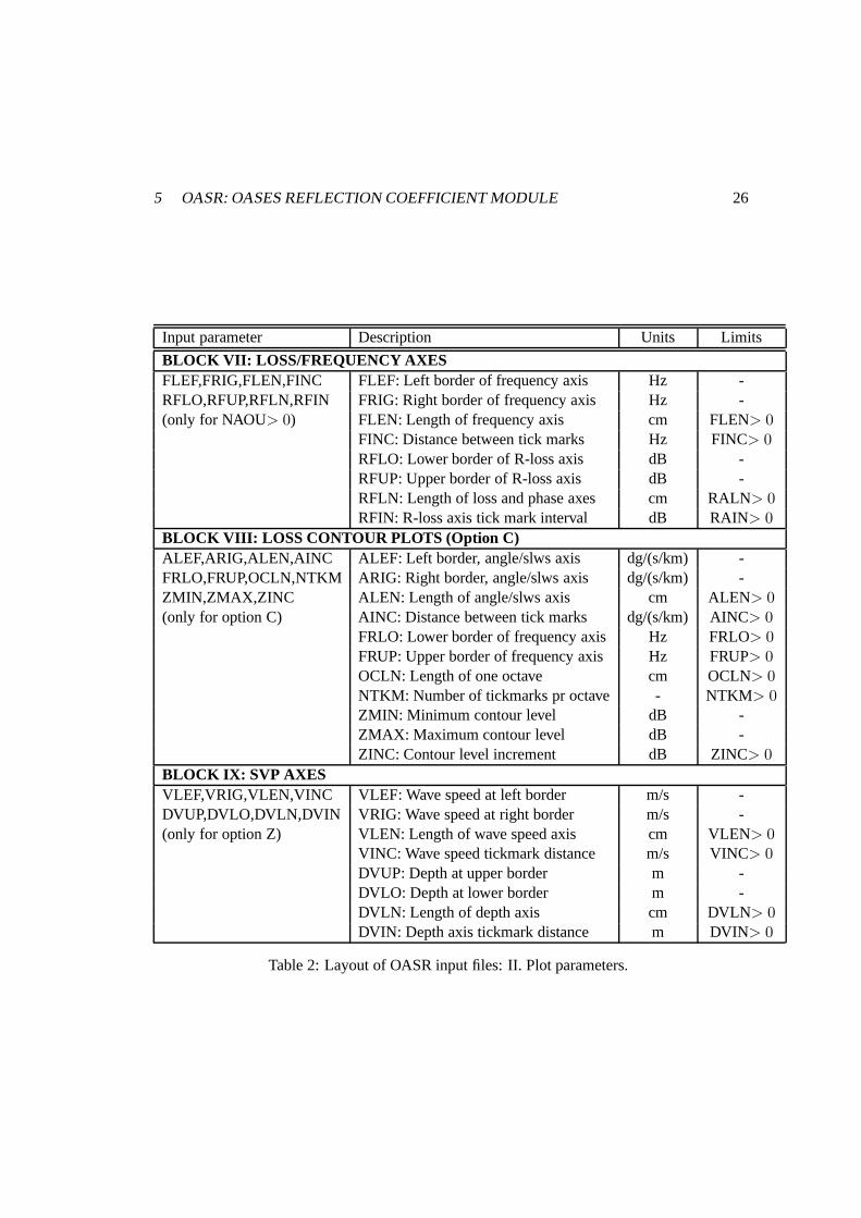
5 OASR: OASES REFLECTION COEFFICIENT MODULE 26
Input parameter Description Units Limits
BLOCK VII: LOSS/FREQUENCY AXESFLEF,FRIG,FLEN,FINC FLEF: Left border of frequency axis Hz -RFLO,RFUP,RFLN,RFIN FRIG: Right border of frequency axis Hz -(only for NAOU> 0) FLEN: Length of frequency axis cm FLEN> 0
FINC: Distance between tick marks Hz FINC> 0RFLO: Lower border of R-loss axis dB -RFUP: Upper border of R-loss axis dB -RFLN: Length of loss and phase axes cm RALN> 0RFIN: R-loss axis tick mark interval dB RAIN> 0
BLOCK VIII: LOSS CONTOUR PLOTS (Option C)ALEF,ARIG,ALEN,AINC ALEF: Left border, angle/slws axis dg/(s/km) -FRLO,FRUP,OCLN,NTKM ARIG: Right border, angle/slws axis dg/(s/km) -ZMIN,ZMAX,ZINC ALEN: Length of angle/slws axis cm ALEN> 0(only for option C) AINC: Distance between tick marks dg/(s/km) AINC> 0
FRLO: Lower border of frequency axis Hz FRLO> 0FRUP: Upper border of frequency axis Hz FRUP> 0OCLN: Length of one octave cm OCLN> 0NTKM: Number of tickmarks pr octave - NTKM> 0ZMIN: Minimum contour level dB -ZMAX: Maximum contour level dB -ZINC: Contour level increment dB ZINC> 0
BLOCK IX: SVP AXESVLEF,VRIG,VLEN,VINC VLEF: Wave speed at left border m/s -DVUP,DVLO,DVLN,DVIN VRIG: Wave speed at right border m/s -(only for option Z) VLEN: Length of wave speed axis cm VLEN> 0
VINC: Wave speed tickmark distance m/s VINC> 0DVUP: Depth at upper border m -DVLO: Depth at lower border m -DVLN: Length of depth axis cm DVLN> 0DVIN: Depth axis tickmark distance m DVIN> 0
Table 2: Layout of OASR input files: II. Plot parameters.

5 OASR: OASES REFLECTION COEFFICIENT MODULE 27
T Generates a table of computed complex reflection coefficients. The file is in ASCIIformat and will be given the same name as the input file, but extension.rco .
Z Plot of velocity profiles.
p Calculates and plots reflection coefficients vs horizontalslowness rather than the defaultgrazing angle. This option allows for computing “reflectioncoefficients” in the evanes-cent regime. When this option is specified, the sampling in Block V should be given inslowness in s/km, and similarly for the plot parameters in Blocks VI and VIII.
s Generates a file with boundary discontinuities for the rough interfaces. Used by OASSfor computing scattering kernels.
t Computes transmission coefficients instead of the defaultreflection coefficients. Thetransmission coefficients refer to the lowermost halfspace.
5.1.3 Block IV: Environmental Model
OASR supports all the environmental models allowed for SAFARI as well as the ones describedabove in Section 4.1. The significance of the standard environmental parameters is as follows
NL: Number of layers, including the upper and lower half-spaces. These should Always beincluded, even in cases where they are vacuum.
D: Depth inm of upper boundary of layer or halfspace. The reference depthcan be choosenarbitrarily, and D() is allowed to be negative. For layer no.1, i.e. the upper half-space,this parameter is dummy.
CC: Velocity of compressional waves inm/s. If specified to 0.0, the layer or half-space isvacuum.
CS: Velocity of shear waves in m/s. If specified to 0.0, the layer or half-space is fluid. IfCS()< 0, it is the compressional velocity at bottom of layer, which is treated as fluidwith 1/c(z)2 linear.
AC: Attennuation of compressional waves indB/λ. If the layer is fluid, and AC() is specifiedto 0.0, then an imperical water attenuation is used (Skretting & Leroy).
AS: Attenuation of shear waves indB/λ
RO: Density ing/cm3.
RG: RMS roughness of interface inm. RG(1) is dummy. If RG< 0 it represents the negativeof the RMS roughness, and the associated correlation lengthCL and spectral exponentshould follow. If RG> 0 the correlation length is assumed to be infinite.

5 OASR: OASES REFLECTION COEFFICIENT MODULE 28
CL: Roughness correlation length in m.
M: Spectral exponent of the power spectrum as defined by Turgut [25], with 1.5 < M ≤ 2.5for realistic surfaces, with M= 1.5 corresponding to the highest roughness, and M= 2.5being a very smooth variation. For 2-D Goff-Jordan surfaces, the fractal dimension isD = 4.5 − M Insignificant for Gaussian spectrum (optiong not specified) but a valuemust be given.
5.2 Execution of OASR
As for FIPR, filenames are passed to OASR via environmental parameters. In Unix systems atypical command fileoasr (in $HOME/oases/bin) is:
# the pound sign invokes the C-shellsetenv FOR001 $1.dat # input filesetenv FOR019 $1.plp # plot parameter filesetenv FOR020 $1.plt # plot data filesetenv FOR028 $1.cdr # contour plot parameter filesetenv FOR029 $1.bdr # contour plot data filesetenv FOR022 $1.rco # reflection coefficient tablesetenv FOR023 $1.trc # reflection coefficient tablesetenv FOR045 $1.rhs # scattering output fileoasr1 # executable
After preparing a data file with the nameinput.dat, OASR is executed by the command:
> oasr input
5.3 Graphics
Command files are provided in a path directory for generatingthe graphics.
To generate curve plots, issue the command:
> mplot input
To generate contour plots, issue the command:
> cplot input

5 OASR: OASES REFLECTION COEFFICIENT MODULE 29
5.4 Output Files
With optionT specified, OAST will generate a file ’input’.rco containg themagnitude|R| andphaseφ of the complex reflection coefficientR = |R| exp φ. Assume you add option T tosaffipr1.dat , and also add option p to select slowness sampling:
SAFARI FIPR case 1.P Z T p30 1500 0 0 0 1 00 1600 400 0.2 0.5 1.8 020 1800 600 0.1 0.2 2.0 050 50 1 10.1 4.0 200 0 # Slowness sampling 0.1 - 4 s/km0 4 20 1 # Slowness axes0 15 12 50 2000 10 1000-20 40 10 20
Then, after issuing the command
> oasr saffipr1
the filesaffipr1.rco will be generated:
50.000 50.000 1 150.000 200 # Frequency, # of slownesses0.100000 0.339462 -15.9968860.119598 0.342714 -15.6405280.139196 0.346415 -15.1964920.158794 0.350498 -14.6550710.178392 0.354880 -14.0064120.197990 0.359469 -13.2407850.217588 0.364159 -12.3490570.237186 0.368833 -11.3225150.256784 0.373363 -10.1530610.276382 0.377615 -8.8328680.295980 0.381445 -7.3540580.315578 0.384707 -5.7079970.335176 0.387249 -3.8839280.354774 0.388919 -1.867177

5 OASR: OASES REFLECTION COEFFICIENT MODULE 30
. . .
. . .
. . .
Note that the reflection coefficients are listed vshorizontal slownessin s/km, and phase anglesare stated indegrees.
Another output fileinput.trc will be generated, identical to theinput.rco file,except for the reflection coefficients being listed vs grazing angle in degrees. The format ofboth these output files is compatible with the one required byOAST as input for optionstandb . The fileinput.trc generated by the input file above is as follows
50.000 50.000 1 2 # fr1, fr2, nf, slowns/angle(1/2)50.000 200 # Frequency, # of angles
81.373070 0.339462 -15.99688679.665359 0.342714 -15.64052877.948311 0.346415 -15.19649276.220207 0.350498 -14.65507174.479210 0.354880 -14.00641272.723396 0.359469 -13.24078570.950676 0.364159 -12.34905769.158813 0.368833 -11.32251567.345337 0.373363 -10.15306165.507576 0.377615 -8.83286863.642544 0.381445 -7.35405861.746929 0.384707 -5.70799759.816971 0.387249 -3.88392857.848427 0.388919 -1.867177
. . .
. . .
. . .
Note that the slowness/angle sampling is identified by the last number in the first line, with 1indicating slowness sampling, and 2 indicating angle sampling.
5.5 OASR - Examples
As an example of the use of OASR for computing seismo-acousticreflection coefficients, thefollowing datafile reproduces the results presented for a sand bottom in Stoll and Kan’s paper[22]:

5 OASR: OASES REFLECTION COEFFICIENT MODULE 31
Figure 1: Reflection coefficients vs frequency and angle for porous sand halfspace, reproducingresults of Stoll and Kan.
Sand. Stoll and Kan 81.N C Z20 1414 0 0 0 1 00 -1800 -600 0.1 0.2 2.0 01. 2.E9 .001 2.65 3.6E10 .47 1.E-10 3.9E-5 2.61E7 4.36E7 1.3 1 .3 1.2510 100000 17 40 90 181 090 0 10 100 15 12 50 90 12 1510 100000 1 11 20 0.50 2000 12 500-10 10 12 5
Assembled in one plot, Fig. 1, the resulting reflection coeffiecients at the 5 frequencies0.01, 0.1, 1, 10, and 100 kHz reproduce exactly the results shown in Fig. 4 of Stoll and Kan’spaper. In addition, the datafile produces the contour plot inFig. 1 of reflection coefficients vsangle and frequency.
OASES handles arbitrary poro-elastic stratifications, andFig. 2(a) shows the equivalentfrequency-angle contours of the reflection coefficient of a 1m thick layer of sand overlying

5 OASR: OASES REFLECTION COEFFICIENT MODULE 32
Figure 2: Reflection coefficients vs frequency and angle for (a) a 1 meter layer of porous sandoverlying a “soft” halfspace, and (b) a 1 meter thick “soft” layer overlying a sand halfspace.Prameters for both media are consistent with those given by Stoll and Kan.
Stoll and Kan’s “soft” sediment. Similarly Fig. 2b) shows the reflection coefficients for a 1meter “soft” layer over sand. The datafile for generating Fig. 2(a) is
1 m Sand over Soft.N C Z30 1414 0 0 0 1 00 -1800 -600 0.1 0.2 2.0 01. 2.E9 .001 2.65 3.6E10 .47 1.E-10 3.9E-5 2.61E7 4.36E7 1.3 1 .3 1.251.0 -1800 -600 0.1 0.2 2.0 01. 2.E9 .001 2.65 3.6E10 .76 1.6E-15 1.56E-7 2.21E7 3.69E7 4. 3 4.3 1.2510 100000 17 40 90 181 090 0 10 100 15 12 50 90 12 1510 100000 1 11 10 0.50 2000 12 500-10 10 12 5
6 OAST: OASES TRANSMISSION LOSS MODULE 33
6 OAST: OASES Transmission Loss Module
Except for the specification of frequencies, OAST is downward compatible with SAFARI-FIPVersion 3.0 and higher, and therefore supports all options and features described in the SAFARImanual. In addition to improved speed and stability, OAST offers several new options.
6.1 Input Files for OAST
The input files for OAST is structured in 12 blocks, as outlined in Tables 3 and 4. In the follow-ing we describe the significance of the various blocks, with particular emphasis on differencesbetween SAFARI-FIP and OAST.
6.1.1 Block I: Title
The title printed on all graphic output generated by OAST.
6.1.2 Block II: OAST options
In addition to supporting the SAFARI options described in [4], OAST supports a wide suite ofnew options.
A Depth-averaged transmission loss plotted for each of the selected field parameters. Theaveraging is performed over the specified number of receivers (block VI).
C Range-depth contour plot for transmission loss. Only allowed for one field parameter ata time.
F In versions earlier than 2.3a Filon-FFT is applied to evaluate the wavenumber integralsinstead of the default FFP. However, this overestimates thetransmission loss and pro-vides no benefit for transmission loss calculations if the sampling criteria are satisfied.In fact it yields up to 3 dB error for automatic sampling and has therefore been disabledin the newer versions of OAST.
G Rough interfaces are assumed to be characterized by a Goff-Jordan power spectrumrather than the default Gaussian.
H Horizontal velocity calculated.
I Hankel transform integrands are plotted for each of the selected field parameters.

6 OAST: OASES TRANSMISSION LOSS MODULE 34
Input parameter Description Units Limits
BLOCK I: TITLETITLE Title of run - ≤ 80 ch.BLOCK II: OPTIONSA B C · · · Output options - ≤ 40 ch.BLOCK III: FREQUENCIESFR1,FR2,NF,COFF,[V] FR1: First frequency Hz > 0
FR2: Last frequency Hz > 0NF: Number of frequencies > 0COFF: Integration contour offset dB/Λ COFF≥ 0V: Source/receiver velocity (only for option d)
BLOCK IV: ENVIRONMENTNL Number of layers, incl. halfspaces - NL≥ 2D,CC,CS,AC,AS,RO,RG,CL D: Depth of interface. m -. CC: Compressional speed m/s CC≥ 0. CS: Shear speed m/s -. AC: Compressional attenuation dB/Λ AC≥ 0. AS: Shear attenuation dB/Λ AS≥ 0
RO: Density g/cm3 RO≥ 0RG: RMS value of interface roughness m -CL: Correlation length of roughness m CL> 0M: Spectral exponent ¿ 1.5
BLOCK V: SOURCESSD,NS,DS,AN,IA,FD,DA SD: Source depth (mean for array) m -
NS: Number of sources in array - NS> 0DS: Vertical source spacing m DS> 0AN: Grazing angle of beam deg -IA: Array type - 1 ≤IA≤ 5FD: Focal depth of beam m FD6=SDDA: Dip angle. (Source type 4). deg -
BLOCK VI: RECEIVERSRD1,RD2,NR,IR RD1: Depth of first receiver m -
RD2: Depth of last receiver m RD2>RD1NR: Number of receivers - NR> 0IR: Plot output increment - IR≥ 0
BLOCK VII: WAVENUMBER SAMPLINGCMIN,CMAX CMIN: Minimum phase velocity m/s CMIN> 0
CMAX: Maximum phase velocity m/s -NW,IC1,IC2 NW: Number of wavenumber samples - NW= 2M ,−1(auto)
IC1: First sampling point - IC1≥ 1IC2: Last sampling point - IC2≤NW
Table 3: Layout of OAST input files: I. Computational parameters.
6 OAST: OASES TRANSMISSION LOSS MODULE 35
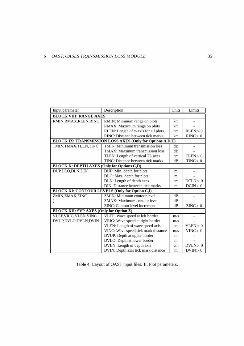
Input parameter Description Units Limits
BLOCK VIII: RANGE AXESRMIN,RMAX,RLEN,RINC RMIN: Minimum range on plots km -
RMAX: Maximum range on plots km -RLEN: Length of x-axis for all plots cm RLEN> 0RINC: Distance between tick marks km RINC> 0
BLOCK IX: TRANSMISSION LOSS AXES (Only for Options A,D,T)TMIN,TMAX,TLEN,TINC TMIN: Minimum transmission loss dB -
TMAX: Maximum transmission loss dB -TLEN: Length of vertical TL axes cm TLEN> 0TINC: Distance between tick marks dB TINC> 0
BLOCK X: DEPTH AXES (Only for Options C,D)DUP,DLO,DLN,DIN DUP: Min. depth for plots m -
DLO: Max. depth for plots m -DLN: Length of depth axes cm DCLN> 0DIN: Distance between tick marks m DCIN> 0
BLOCK XI: CONTOUR LEVELS (Only for Option C,f)ZMIN,ZMAX,ZINC ZMIN: Minimum contour level dB -( ZMAX: Maximum contour level dB -
ZINC: Contour level increment dB ZINC> 0BLOCK XII: SVP AXES (Only for Option Z)VLEF,VRIG,VLEN,VINC VLEF: Wave speed at left border m/s -DVUP,DVLO,DVLN,DVIN VRIG: Wave speed at right border m/s -
VLEN: Length of wave speed axis cm VLEN> 0VINC: Wave speed tick mark distance m/s VINC> 0DVUP: Depth at upper border m -DVLO: Depth at lower border m -DVLN: Length of depth axis cm DVLN> 0DVIN: Depth axis tick mark distance m DVIN> 0
Table 4: Layout of OAST input files: II. Plot parameters.

6 OAST: OASES TRANSMISSION LOSS MODULE 36
J Complex integration contour. The contour is shifted into the upper halfpane by an offsetcontrolled by the input parameter COFF (Block III).
K Computes the bulk pressure. In elastic media the bulk pressure only has contributionsfrom the compressional potential. In fluid media the bulk pressure is equal to the acousticpressure. Therefore for fluids this option yields the negative of the result produced byoption N or R.
L Linear vertical source array.
N Normal stressσzz (= −p in fluids) calculated.
P Plane geometry. The sources will be line-sources instead ofpoint-sources as used in thedefault cylindrical geometry.
R Computes the radial normal stressσrr (or σxx for plane geometry).
S Computes the stress equivalent of the shear potential in elastic media. This is an angle-independent measure, proportional to the shear potential,with no contribution from thecompressional potential (in contrast to shear stress on a particular plane). For fluids thisoption yields zero.
T Transmission loss plotted as function of range for each of the selected field parameters.
V Vertical velocity calculated.
Z Plot of velocity profile.
a Angular spectra of the integration kernels are plotted. A0 − 90◦ axis is automaticallyselected representing the grazing angle (0◦ corresponds to horizontal propagation ).NOTE: The same wavenumber corresponds to different grazingangles in different me-dia!. The vertical axis is selected automatically, representing the angular density (asopposed to the wavenumber density for integrand plots ( option I ).
b Solves the depth-separated wave equation with the lowermost interface condition ex-pressed in terms of a complex reflection coefficient. The reflection coefficient must betabulated in a input fileinput.trc which may either be produced from experimentaldata or by the reflection coefficient module OASR as describedon Page 30. See alsothere for the file format. The lower halfspace must be specified as vacuum and the lastlayer as an isovelocity fluid without sources for this option. Add dummy layer if nec-essary. Further, the frequency sampling must be consistent. Therefore, if this option iscombined with optionf , the input file must have cosistent logarithmic sampling. UsingOASR this is optained by using optionC with the same minimum and maximum fre-quencies, and number of frequencies. Note: Care should be taken using this option with acomplex integration contour, optionJ . The tabulated reflection coefficient must clearlycorrespond to the same imaginary wavenumber components forOAST to yield properresults.OASR calculates the reflection coefficient for real horizontal wavenumbers.

6 OAST: OASES TRANSMISSION LOSS MODULE 37
c Contours of integration kernels as function of horizontal wavenumber (abcissa) andreceiver depth (ordinate). The horizontal wavenumber axisis selected automatically,whereas the depth axis is plotted according to the parameters given for option C. Thecontour levels are determined automatically.
d Source/receiver dynamics. OAST v 1.7 handles the problem ofsource and receiver mov-ing through the waveguide at the same speed and direction. The velocity projection Vonto the line connecting source and receiver must be specified in Block III, as shown intable 3. Since source and receiver are moving at identical speeds there is no Dopplershift, but the Green’s function is different from the staticone, as described by Schmidtand Kuperman[9].
f A full Hankel transform integration scheme is used for low values ofkr and taperedinto the FFP integration used for largekr. The compensation is achieved at very lowcomputational cost and is recommended highly for cases where the near field is needed.
o Contours of transmission loss plotted vs frequency and range, i.e. the traditional ’op-timum frequency’ contour plots. Requires NFREQ> 1 (see below). A logarithmicfrequency axis is assumed for this option. Requires ZMIN, ZMAX and ZINC to bespecified in Block XII (same contour levels as for optionC which may be specifiedsimultaneously).
g Rough interfaces are assumed to be characterized by a Goff-Jordan power spectrumrather than the default Gaussian (Same as G).
l User defined source array. This new option is similar to option L in the sense that thatit introduces a vertical source array of time delayed sources of identical type. However,this option allows the depth, amplitude and delay time to be be specified individually foreach source in the array. The source data should be provided in a separate file,input.src,in the format described below in Section 6.1.5.
s Outputs the mean field discontinuity at a rough interface to the file ’input’.rhs for inputto the reverberation model OASS.
t Solves the depth-separated wave equation with the top interface condition expressed interms of a complex reflection coefficient. The reflection coefficient must be tabulated ina input file input.trc which may either be produced from experimental data or bythe reflection coefficient moduleOASR as described on Page 30. See also there for thefile format. The upper halfspace must be specified as vacuum and the first layer as anisovelocity fluid without sources for this option. Add dummylayer if necessary. Further,the frequency sampling must be consistent. Therefore, if this option is combined withoption f , the input file must have cosistent logarithmic sampling. Using OASR thisis optained by using optionC with the same minimum and maximum frequencies, andnumber of frequencies. Note: Care should be taken using thisoption with a complex in-tegration contour, optionJ . The tabulated reflection coefficient must clearly correspond
6 OAST: OASES TRANSMISSION LOSS MODULE 38
to the same imaginary wavenumber components forOAST to yield proper results.OASRcalculates the reflection coefficient for real horizontal wavenumbers.
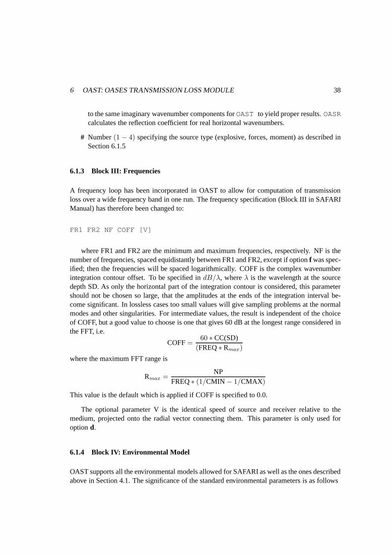
# Number(1 − 4) specifying the source type (explosive, forces, moment) as described inSection 6.1.5
6.1.3 Block III: Frequencies
A frequency loop has been incorporated in OAST to allow for computation of transmissionloss over a wide frequency band in one run. The frequency specification (Block III in SAFARIManual) has therefore been changed to:
FR1 FR2 NF COFF [V]
where FR1 and FR2 are the minimum and maximum frequencies, respectively. NF is thenumber of frequencies, spaced equidistantly between FR1 and FR2, except if optionf was spec-ified; then the frequencies will be spaced logarithmically.COFF is the complex wavenumberintegration contour offset. To be specified indB/λ, whereλ is the wavelength at the sourcedepth SD. As only the horizontal part of the integration contour is considered, this parametershould not be chosen so large, that the amplitudes at the endsof the integration interval be-come significant. In lossless cases too small values will give sampling problems at the normalmodes and other singularities. For intermediate values, the result is independent of the choiceof COFF, but a good value to choose is one that gives 60 dB at thelongest range considered inthe FFT, i.e.
COFF=60 ∗ CC(SD)
(FREQ∗ Rmax)
where the maximum FFT range is
Rmax =NP
FREQ∗ (1/CMIN − 1/CMAX)
This value is the default which is applied if COFF is specifiedto 0.0.
The optional parameter V is the identical speed of source andreceiver relative to themedium, projected onto the radial vector connecting them. This parameter is only used foroptiond.
6.1.4 Block IV: Environmental Model
OAST supports all the environmental models allowed for SAFARI as well as the ones describedabove in Section 4.1. The significance of the standard environmental parameters is as follows

6 OAST: OASES TRANSMISSION LOSS MODULE 39
NL: Number of layers, including the upper and lower half-spaces. These should Always beincluded, even in cases where they are vacuum.
D: Depth inm of upper boundary of layer or halfspace. The reference depthcan be choosenarbitrarily, and D() is allowed to be negative. For layer no.1, i.e. the upper half-space,this parameter is dummy.
CC: Velocity of compressional waves inm/s. If specified to 0.0, the layer or half-space isvacuum.
CS: Velocity of shear waves in m/s. If specified to 0.0, the layer or half-space is fluid. IfCS()< 0, it is the compressional velocity at bottom of layer, which is treated as fluidwith 1/c(z)2 linear.
AC: Attennuation of compressional waves indB/λ. If the layer is fluid, and AC() is specifiedto 0.0, then an imperical water attenuation is used (Skretting & Leroy).
AS: Attenuation of shear waves indB/λ
RO: Density ing/cm3.
RG: RMS roughness of interface inm. RG(1) is dummy. If RG< 0 it represents the negativeof the RMS roughness, and the associated correlation lengthCL and spectral exponmentM should follow. If RG> 0 the correlation length is assumed to be infinite.
CL: Roughness correlation length in m.
M: Spectral exponent of the power spectrum as defined by Turgut [25], with 1.5 < M ≤ 2.5for realistic surfaces, with M= 1.5 corresponding to the highest roughness, and M= 2.5being a very smooth variation. For 2-D Goff-Jordan surfaces, the fractal dimension isD = 4.5 − M Insignificant for Gaussian spectrum (optiong not specified) but a valuemust be given.
6.1.5 Block V: Sources
OAST supports the same sources as SAFARI-FIP, i.e explosivesources in fluids or solids orvertical point forces in solids (option X). Multible sources in a vertical array are supported. Ifsources with horizontal directionality are desired, the 3-dimensional version OASP3D must beused. The significance of the source parameters are as follows
SD: Source depth inm. If option ’L’ has been specified, then SD defines the mid-point of thevertical source array.
NS: Number of sources in the array.

6 OAST: OASES TRANSMISSION LOSS MODULE 40
DS: Source spacing inm.
AN: Specifies the nominal grazing ANG of the generated beam indegrees.ANG > 0 corre-sponds to downward propagation.
IA: Array type
1. Rectangular weighted array
2. Hanning weighted array
3. Hanning weighted focusing array
4. Gaussian weighted array
5. Gaussian weighted focusing array
FD: Focal depth inm for an array of type 3 and 5.
DA: Dip angle in degrees for dip-slip sources (type 4).
Source Types
As in SAFARI the default source type in OAST is an explosive type compressional source.In addition to the optional vertical point force, and axisymmetric seismic moment source hasbeen added to OAST. The source type is specified by a number(1− 3) in the option field (line2). The translation is as follows:
1. Explosive source (default) normalized to unit pressure at 1 m distance.
2. Vertical point force with amplitude 1 N.
3. Horizontal (in-plane) point force with amplitude 1 N.
4. Dip-slip source with seismic moment 1 Nm. Dip angle specified in degrees in block V,following the other parameters.
5. Omnidirectional seismic moment source representing explosive source. Same as type 1,but all three force dipoles have seismic moment 1 Nm.
Source Normalization
In SAFARI, the source strength was normalized to yield unit pressure (in Pa) at a distanceof 1 m from the source (for solids the negative of the normal stress 1 m below the source).
In OASES, the same source normalization has been maintainedfor point sources (explosivesources) in fluid media. For solid media, however, the sources are normalized to unit volume(1 m3) injection for explosive sources and unit force 1 N for pointsources or 1 N/m for linesources.

6 OAST: OASES TRANSMISSION LOSS MODULE 41
User defined Source Arrays
Version 1.6 of OAST has been upgraded to allow a user-defined source array through optionl.
Option l is intended for general physical arrays with uneven spacingor special shadings,As for the built-in arrays, such user-defined arrays may be present in fluid as well as elasticmedia. The array definition should be given in the fileinput.src in the following format
LSSDC(1) SDELAY(1) SSTREN(1) # Depth (m), Delay (s), Amplitud eSDC(2) SDELAY(2) SSTREN(2)SDC(3) SDELAY(3) SSTREN(3)
: : :: : :
SDC(LS) SDELAY(LS) SSTREN(LS)
6.1.6 Block VI: Receivers
The default specification of the receiver depths is the same as for SAFARI, i.e. through theparameters RD1, RD2, NR and IR in Block VI, with
RD1 Depth of uppermost receiver in m
RD2 Depth of lowermost receiver in m
NR Number of receiver depths
IR Depth increment for options I and T
By default, the NR receivers are placed equidistantly in thevertical.
Non-equidistant Receiver Depths
In OASES the receiver depths can optionally be specified individually. The parameter NRis used as a flag for this option. Thus, if NR< 0 the number of receivers is interpreted as –NR,with the individual depths following immidiately following Block VI. As an example, SAFARIFIP case 2 with receivers at 100, 105 and 120 m is run with the following data file:
SAFARI-FIP case 2.N I T J Z30 30 1 05

6 OAST: OASES TRANSMISSION LOSS MODULE 42
0 0 0 0 0 0 00 1500 -1480 0 0 1 0
30 1480 -1490 0 0 1 0100 1600 400 0.2 0.5 1.8 0120 1800 600 0.1 0.2 2.0 050100 100 -3 1 # 3 receiver depths100.0 105.0 120.0 # Receiver depths in meters700 1E81024 1 512
0 5 20 120 80 12 101450 1550 10 25
0 100 10 20
6.1.7 Block VII: Wavenumber Integration
This block specifies the wavenumber sampling in the standardSAFARI format. The criticalissues involved in selecting the wavenumber sampling is described in the SAFARI manual [4],but even more detailed inComputational Ocean Acoustics[3]. The structure of this input blockis as follows:
CMIN: Minimum phase velocity in m/s. Determines the upper limit of the truncated horizontalwave- number space:
kmax =2π ∗ FREQ
CMIN
CMAX: Maximum phase velocity in m/s. Determines the lower limit of the truncated horizontalwave- number space:
kmin =2π ∗ FREQ
CMAXIn plane geometry ( option P ) CMAX may be specified as negative. In this case, thenegative wavenumber spectrum will be included withkmin = −kmax, yielding correctsolution also at zero range. In contrast to SAFARI, OAST allows for complex contourintegration (option J) in this case.
NW: Number of sampling points in wavenumber space. Should bean integer power of 2, i.e.NWN= 2m. The sampling points are placed equidistantly in the truncated wavenumberspace determined by CMIN and CMAX.
IC1: Number of the first sampling point, where the calculation is to be performed. If IC1> 1,then the Hankel transform is zeroed for sampling points 1,2. . .IC1-1, and the disconti-nuity is smoothed.
6 OAST: OASES TRANSMISSION LOSS MODULE 43
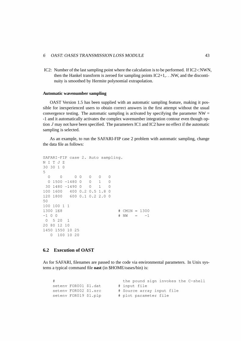
IC2: Number of the last sampling point where the calculationis to be performed. If IC2<NWN,then the Hankel transform is zeroed for sampling points IC2+1,. . .NW, and the disconti-nuity is smoothed by Hermite polynomial extrapolation.
Automatic wavenumber sampling
OAST Version 1.5 has been supplied with an automatic sampling feature, making it pos-sible for inexperienced users to obtain correct answers in the first attempt without the usualconvergence testing. The automatic sampling is activated by specifying the parameter NW =-1 and it automatically activates the complex wavenumber integration contour even though op-tion J may not have been specified. The parameters IC1 and IC2 have noeffect if the automaticsampling is selected.
As an example, to run the SAFARI-FIP case 2 problem with automatic sampling, changethe data file as follows:
SAFARI-FIP case 2. Auto sampling.N I T J Z30 30 1 05
0 0 0 0 0 0 00 1500 -1480 0 0 1 0
30 1480 -1490 0 0 1 0100 1600 400 0.2 0.5 1.8 0120 1800 600 0.1 0.2 2.0 050100 100 1 11300 1E8 # CMIN = 1300-1 0 0 # NW = -1
0 5 20 120 80 12 101450 1550 10 25
0 100 10 20
6.2 Execution of OAST
As for SAFARI, filenames are passed to the code via environmental parameters. In Unix sys-tems a typical command fileoast (in $HOME/oases/bin) is:
# the pound sign invokes the C-shellsetenv FOR001 $1.dat # input filesetenv FOR002 $1.src # Source array input filesetenv FOR019 $1.plp # plot parameter file

6 OAST: OASES TRANSMISSION LOSS MODULE 44
setenv FOR020 $1.plt # plot data filesetenv FOR023 $1.trc # reflection coefficient table (input )setenv FOR028 $1.cdr # contour plot parameter filesetenv FOR029 $1.bdr # contour plot data filesetenv FOR045 $1.rhs # file for scattering discontinuitiesoast2 # executable
After preparing a data file with the nameinput.dat, OAST is executed by the command:
> oast input
6.3 Graphics
Command files are provided in a path directory for generatingthe graphics.
To generate curve plots, issue the command:
> mplot input
To generate contour plots, issue the command:
> cplot input

7 RDOAST: OASES RANGE-DEPENDENT TL MODULE 45
7 RDOAST: OASES Range-dependent TL Module
RDOASTis the range-dependentversion ofOAST. RDOASTuses a Virtual Source Ap-proach for coupling the field between range-independent sectors, basically using averticalsource/receiver array, and asingle-scatter, local plane wavehandling of vertical discontinu-ities. In contrast to the similar approach of the elastic PE,VISA properly handles seismicconversion at the vertical boundaries. The solutions compare extremely well with PE solutionsfor week contrast problems, and with full boundary integralapproaches for several canonicalelastic benchmark problems [20, 21].
7.1 Input Files for RDOAST
The input files forRDOASTare very similar to those ofOAST , with the main differencesbeing the extra environmental blocks, and two receiver specifications, one for the marchingsource/receiver array and contour plots, and one for TL vs range etc. As for OAST, the inputfile is structured in 12 blocks, as outlined in Tables 5 and 6.
7.1.1 Block I: Title
The title printed on all graphic output generated by RDOAST.
7.1.2 Block II: RDOAST options
In addition to supporting all the OAST options, RDOAST has a few additional ones.
A Depth-averaged transmission loss plotted for each of the selected field parameters. Theaveraging is performed over the specified number of receivers (block VI).
B Computes backscattered field in single-scatter approximation.
C Range-depth contour plot for transmission loss. Only allowed for one field parameter ata time.
F This option activates the FFP integration within each sector. The default is direct inte-gration. Use option F only in cases where each sector has a large number of receiverranges (∆R = 2π/(kmax − kmin)). Note that the effect of this option is different thanin OAST.
G Rough interfaces are assumed to be characterized by a Goff-Jordan power spectrumrather than the default Gaussian.

7 RDOAST: OASES RANGE-DEPENDENT TL MODULE 46
Input parameter Description Units Limits
BLOCK I: TITLETITLE Title of run - ≤ 80 ch.BLOCK II: OPTIONSA B C · · · Output options - ≤ 40 ch.BLOCK III: FREQUENCIESFR1,FR2,NF,COFF,[V] FR1: First frequency Hz > 0
FR2: Last frequency Hz > 0NF: Number of frequencies > 0COFF: Integration contour offset dB/Λ COFF≥ 0V: Source/receiver velocity (only for option d)
BLOCK IV: ENVIRONMENTNSEC Number of sectors - NSEC≥ 1NL, SECL Sector 1: No. layers, length -, km NL≥ 2D,CC,CS,AC,AS,RO,RG,CL D: Depth of interface. m -. CC: Compressional speed m/s CC≥ 0. CS: Shear speed m/s -. AC: Compressional attenuation dB/Λ AC≥ 0. AS: Shear attenuation dB/Λ AS≥ 0
RO: Density g/cm3 RO≥ 0RG: RMS value of interface roughness m -CL: Correlation length of roughness m CL> 0
NL, SECL Sector 2: No. layers, length -, km NL≥ 2D,CC,CS,AC,AS,RO,RG,CL -..BLOCK V: SOURCESSD,NS,DS,AN,IA,FD,DA SD: Source depth (mean for array) m -
NS: Number of sources in array - NS> 0DS: Vertical source spacing m DS> 0AN: Grazing angle of beam deg -IA: Array type - 1 ≤IA≤ 5FD: Focal depth of beam m FD6=SDDA: Dip angle. (Source type 4). deg -
BLOCK VI: RECEIVERSRD1,RD2,NR RD1: Depth of first receiver m -
RD2: Depth of last receiver m RD2>RD1NR: Number of receivers - NR> 0
D1,D2,ND: Depth sampling opt I, T etc.BLOCK VII: WAVENUMBER SAMPLINGCMIN,CMAX CMIN: Minimum phase velocity m/s CMIN> 0
CMAX: Maximum phase velocity m/s -NW,IC1,IC2 NW: Number of wavenumber samples - NW= 2M ,−1(auto)
IC1: First sampling point - IC1≥ 1IC2: Last sampling point - IC2≤NW
Table 5: Layout of RDOAST input files: I. Computational parameters.

7 RDOAST: OASES RANGE-DEPENDENT TL MODULE 47
Input parameter Description Units Limits
BLOCK VIII: RANGE AXESRMIN,RMAX,RLEN,RINC RMIN: Minimum range on plots km -
RMAX: Maximum range on plots km -RLEN: Length of x-axis for all plots cm RLEN> 0RINC: Distance between tick marks km RINC> 0
BLOCK IX: TRANSMISSION LOSS AXES (Only for Options A,D,T)TMIN,TMAX,TLEN,TINC TMIN: Minimum transmission loss dB -
TMAX: Maximum transmission loss dB -TLEN: Length of vertical TL axes cm TLEN> 0TINC: Distance between tick marks dB TINC> 0
BLOCK X: DEPTH AXES (Only for Options C,D)DUP,DLO,DLN,DIN DUP: Min. depth for plots m -
DLO: Max. depth for plots m -DLN: Length of depth axes cm DCLN> 0DIN: Distance between tick marks m DCIN> 0
BLOCK XI: CONTOUR LEVELS (Only for Option C,f)ZMIN,ZMAX,ZINC ZMIN: Minimum contour level dB -( ZMAX: Maximum contour level dB -
ZINC: Contour level increment dB ZINC> 0BLOCK XII: SVP AXES (Only for Option Z)VLEF,VRIG,VLEN,VINC VLEF: Wave speed at left border m/s -DVUP,DVLO,DVLN,DVIN VRIG: Wave speed at right border m/s -
VLEN: Length of wave speed axis cm VLEN> 0VINC: Wave speed tick mark distance m/s VINC> 0DVUP: Depth at upper border m -DVLO: Depth at lower border m -DVLN: Length of depth axis cm DVLN> 0DVIN: Depth axis tick mark distance m DVIN> 0
Table 6: Layout of RDOAST input files: II. Plot parameters.

7 RDOAST: OASES RANGE-DEPENDENT TL MODULE 48
H Horizontal velocity calculated.
I Hankel transform integrands are plotted for each of the selected field parameters.
J Complex integration contour. The contour is shifted into the upper halfpane by an offsetcontrolled by the input parameter COFF (Block III).
K Computes the bulk pressure. In elastic media the bulk pressure only has contributionsfrom the compressional potential. In fluid media the bulk pressure is equal to the acousticpressure. Therefore for fluids this option yields the negative of the result produced byoption N or R.
L Linear vertical source array.
N Normal stressσzz (= −p in fluids) calculated.
P Plane geometry. The sources will be line-sources instead ofpoint-sources as used in thedefault cylindrical geometry.
R Computes the radial normal stressσrr (or σxx for plane geometry).
S Computes the stress equivalent of the shear potential in elastic media. This is an angle-independent measure, proportional to the shear potential,with no contribution from thecompressional potential (in contrast to shear stress on a particular plane). For fluids thisoption yields zero.
T Transmission loss plotted as function of range for each of the selected field parameters.
V Vertical velocity calculated.
Z Plot of velocity profile.
a Angular spectra of the integration kernels are plotted. A0 − 90◦ axis is automaticallyselected representing the grazing angle (0◦ corresponds to horizontal propagation ).NOTE: The same wavenumber corresponds to different grazingangles in different me-dia!. The vertical axis is selected automatically, representing the angular density (asopposed to the wavenumber density for integrand plots ( option I ).
b Solves the depth-separated wave equation with the lowermost interface condition ex-pressed in terms of a complex reflection coefficient. The reflection coefficient must betabulated in a input fileinput.trc which may either be produced from experimentaldata or by the reflection coefficient module OASR as describedon Page 30. See alsothere for the file format. The lower halfspace must be specified as vacuum and the lastlayer as an isovelocity fluid without sources for this option. Add dummy layer if nec-essary. Further, the frequency sampling must be consistent. Therefore, if this option iscombined with optionf , the input file must have cosistent logarithmic sampling. Using
7 RDOAST: OASES RANGE-DEPENDENT TL MODULE 49
OASR this is optained by using optionC with the same minimum and maximum fre-quencies, and number of frequencies. Note: Care should be taken using this option with acomplex integration contour, optionJ . The tabulated reflection coefficient must clearlycorrespond to the same imaginary wavenumber components forOAST to yield properresults.OASR calculates the reflection coefficient for real horizontal wavenumbers.
c Contours of integration kernels as function of horizontal wavenumber (abcissa) andreceiver depth (ordinate). The horizontal wavenumber axisis selected automatically,whereas the depth axis is plotted according to the parameters given for option C. Thecontour levels are determined automatically.
d Source/receiver dynamics. OAST v 1.7 handles the problem ofsource and receiver mov-ing through the waveguide at the same speed and direction. The velocity projection Vonto the line connecting source and receiver must be specified in Block III, as shown intable 3. Since source and receiver are moving at identical speeds there is no Dopplershift, but the Green’s function is different from the staticone, as described by Schmidtand Kuperman[9].
f Contours of transmission loss plotted vs frequency and range. Requires NFREQ> 0(see below). A logarithmic frequency axis is assumed for this option. Requires ZMIN,ZMAX and ZINC to be specified in Block XII (same contour levelsas for optionCwhich may be specified simultaneously).
g Rough interfaces are assumed to be characterized by a Goff-Jordan power spectrumrather than the default Gaussian (Same as G).
l User defined source array. This new option is similar to option L in the sense that thatit introduces a vertical source array of time delayed sources of identical type. However,this option allows the depth, amplitude and delay time to be be specified individually foreach source in the array. The source data should be provided in a separate file,input.src,in the format described below in Section 7.1.5.
s Outputs the mean field discontinuity at a rough interface to the file ’input’.rhs for inputto the reverberation model OASS.
t Solves the depth-separated wave equation with the top interface condition expressed interms of a complex reflection coefficient. The reflection coefficient must be tabulated ina input file input.trc which may either be produced from experimental data or bythe reflection coefficient moduleOASR as described on Page 30. See also there for thefile format. The upper halfspace must be specified as vacuum and the first layer as anisovelocity fluid without sources for this option. Add dummylayer if necessary. Further,the frequency sampling must be consistent. Therefore, if this option is combined withoption f , the input file must have cosistent logarithmic sampling. Using OASR thisis optained by using optionC with the same minimum and maximum frequencies, and

7 RDOAST: OASES RANGE-DEPENDENT TL MODULE 50
number of frequencies. Note: Care should be taken using thisoption with a complex in-tegration contour, optionJ . The tabulated reflection coefficient must clearly correspondto the same imaginary wavenumber components forOAST to yield proper results.OASRcalculates the reflection coefficient for real horizontal wavenumbers.
# Number(1 − 4) specifying the source type (explosive, forces, moment) as described inSection 7.1.5
7.1.3 Block III: Frequencies
A frequency loop has been incorporated in OAST to allow for computation of transmissionloss over a wide frequency band in one run. The frequency specification (Block III in SAFARIManual) has therefore been changed to:
FR1 FR2 NF COFF [V]
where FR1 and FR2 are the minimum and maximum frequencies, respectively. NF is thenumber of frequencies, spaced equidistantly between FR1 and FR2, except if optionf was spec-ified; then the frequencies will be spaced logarithmically.COFF is the complex wavenumberintegration contour offset. To be specified indB/λ, whereλ is the wavelength at the sourcedepth SD. As only the horizontal part of the integration contour is considered, this parametershould not be chosen so large, that the amplitudes at the endsof the integration interval be-come significant. In lossless cases too small values will give sampling problems at the normalmodes and other singularities. For intermediate values, the result is independent of the choiceof COFF, but a good value to choose is one that gives 60 dB at thelongest range considered inthe FFT, i.e.
COFF=60 ∗ CC(SD)
(FREQ∗ Rmax)
where the maximum FFT range is
Rmax =NP
FREQ∗ (1/CMIN − 1/CMAX)
This value is the default which is applied if COFF is specifiedto 0.0.
The optional parameter V is the identical speed of source andreceiver relative to themedium, projected onto the radial vector connecting them. This parameter is only used foroptiond.

7 RDOAST: OASES RANGE-DEPENDENT TL MODULE 51
7.1.4 Block IV: Environmental Model
RDOAST supports all the environmental models allowed for SAFARI as well as the ones de-scribed above in Section 4.1. The stepwize range-independent environment is specified by astandard OAST environment block for eac sector, with the length of the sector added to the linecontaining the number of layers. The sector length is given in kilometers. The significance ofthe environmental parameters is as follows
NSEC: Number of sectors, each of which should have a block with layer data in input file.
NL: Number of layers, including the upper and lower half-spaces. These should Always beincluded, even in cases where they are vacuum.
SECL: Length of sector in kilometers.
D: Depth inm of upper boundary of layer or halfspace. The reference depthcan be choosenarbitrarily, and D() is allowed to be negative. For layer no.1, i.e. the upper half-space,this parameter is dummy.
CC: Velocity of compressional waves inm/s. If specified to 0.0, the layer or half-space isvacuum.
CS: Velocity of shear waves in m/s. If specified to 0.0, the layer or half-space is fluid. IfCS()< 0, it is the compressional velocity at bottom of layer, which is treated as fluidwith 1/c(z)2 linear.
AC: Attennuation of compressional waves indB/λ. If the layer is fluid, and AC() is specifiedto 0.0, then an imperical water attenuation is used (Skretting & Leroy).
AS: Attenuation of shear waves indB/λ
RO: Density ing/cm3.
RG: RMS roughness of interface inm. RG(1) is dummy. If RG< 0 it represents the negativeof the RMS roughness, and the associated correlation lengthCL should follow. If RG> 0the correlation length is assumed to be infinite.
CL: Roughness correlation length in m.
7.1.5 Block V: Sources
RDOAST supports the same sources as OAST. Multible sources in a vertical array are sup-ported. The significance of the source parameters are as follows

7 RDOAST: OASES RANGE-DEPENDENT TL MODULE 52
SD: Source depth inm. If option ’L’ has been specified, then SD defines the mid-point of thevertical source array.
NS: Number of sources in the array.
DS: Source spacing inm.
AN: Specifies the nominal grazing ANG of the generated beam indegrees.ANG > 0 corre-sponds to downward propagation.
IA: Array type
1. Rectangular weighted array
2. Hanning weighted array
3. Hanning weighted focusing array
4. Gaussian weighted array
5. Gaussian weighted focusing array
FD: Focal depth inm for an array of type 3 and 5.
DA: Dip angle in degrees for dip-slip sources (type 4).
Source Types
As in SAFARI the default source type in OAST is an explosive type compressional source.In addition to the optional vertical point force, and axisymmetric seismic moment source hasbeen added to OAST. The source type is specified by a number(1− 5) in the option field (line2). The translation is as follows:
1. Explosive source (default) normalized to unit pressure at 1 m distance.
2. Vertical point force with amplitude 1 N.
3. Horizontal (in-plane) point force with amplitude 1 N.
4. Dip-slip source with seismic moment 1 Nm. Dip angle specified in degrees in block V,following the other parameters.
5. Omnidirectional seismic moment source representing explosive source. Same as type 1,but all three force dipoles have seismic moment 1 Nm.
Source Normalization
In SAFARI, the source strength was normalized to yield unit pressure (in Pa) at a distanceof 1 m from the source (for solids the negative of the normal stress 1 m below the source).

7 RDOAST: OASES RANGE-DEPENDENT TL MODULE 53
In OASES, the same source normalization has been maintainedfor point sources (explosivesources) in fluid media. For solid media, however, the sources are normalized to unit volume(1 m3) injection for explosive sources and unit force 1 N for pointsources or 1 N/m for linesources.
User defined Source Arrays
Version 1.6 of OAST has been upgraded to allow a user-defined source array through optionl.
Option l is intended for general physical arrays with uneven spacingor special shadings,As for the built-in arrays, such user-defined arrays may be present in fluid as well as elasticmedia. The array definition should be given in the fileinput.src in the following format
LSSDC(1) SDELAY(1) SSTREN(1) # Depth (m), Delay (s), Amplitud eSDC(2) SDELAY(2) SSTREN(2)SDC(3) SDELAY(3) SSTREN(3)
: : :: : :
SDC(LS) SDELAY(LS) SSTREN(LS)
7.1.6 Block VI: Receivers
The specification of the receiver depths is slightly different than for OAST, with two recordsinstead of one. The significance of the parameters is
RD1 Depth of uppermost source/receiver in vertical field matching arrays in meters.
RD2 Depth of lowermost source/receiver in vertical field matching arrays in meters.
NR Number of source/receiver depths.
D1 Depth of uppermost receiver for which integrands and/or TL plots should be generated .Will be modified to closest depth in receiver array specified by RD1, RD2, and NR.
D2 Depth of lowermost receiver for which integrands and/or TL plots should be generated.Will be modified to closest depth in receiver array specified by RD1, RD2, and NR.
ND Number of equidistant depths for which integrands and/orTL will be plotted.
By default, the NR and ND receivers are placed equidistantlyin the vertical. Note thatthe vertical source/receiver arrays provide the only mechaanism for the field to propagate.Therefore, RD1 and RD2 must be chosen carefully. E.g. RD2 must be deep enough into the

7 RDOAST: OASES RANGE-DEPENDENT TL MODULE 54
lower halfspace to include all significant upward radiatingfield. NR must be large enough tosample the vertical field distribution, i.e. denser than half the shortest vertical wavelength.
Non-equidistant Receiver Depths
In RDOASES the source/receiver depths can optionally be specified individually. The pa-rameter NR is used as a flag for this option. Thus, if NR< 0 the number of receivers isinterpreted as –NR, with the individual depths following immidiately following Block VI.
7.1.7 Block VII: Wavenumber Integration
This block specifies the wavenumber sampling in the standardSAFARI format. The criticalissues involved in selecting the wavenumber sampling is described in the SAFARI manual [4],but even more detailed inComputational Ocean Acoustics[3]. The structure of this input blockis as follows:
CMIN: Minimum phase velocity in m/s. Determines the upper limit of the truncated horizontalwave- number space:
kmax =2π ∗ FREQ
CMIN
CMAX: Maximum phase velocity in m/s. Determines the lower limit of the truncated horizontalwave- number space:
kmin =2π ∗ FREQ
CMAXIn plane geometry ( option P ) CMAX may be specified as negative. In this case, thenegative wavenumber spectrum will be included withkmin = −kmax, yielding correctsolution also at zero range. In contrast to SAFARI, OAST allows for complex contourintegration (option J) in this case.
NW: Number of sampling points in wavenumber space. Should bean integer power of 2, i.e.NWN= 2m. The sampling points are placed equidistantly in the truncated wavenumberspace determined by CMIN and CMAX.
IC1: Number of the first sampling point, where the calculation is to be performed. If IC1> 1,then the Hankel transform is zeroed for sampling points 1,2. . .IC1-1, and the disconti-nuity is smoothed.
IC2: Number of the last sampling point where the calculationis to be performed. If IC2<NWN,then the Hankel transform is zeroed for sampling points IC2+1,. . .NW, and the disconti-nuity is smoothed by Hermite polynomial extrapolation.
Automatic wavenumber sampling

7 RDOAST: OASES RANGE-DEPENDENT TL MODULE 55
RDOAST supports the standard OAST auto sampling option. Theautomatic samplingis activated by specifying the parameter NW = -1 and it automatically activates the complexwavenumber integration contour even though optionJ may not have been specified. The pa-rameters IC1 and IC2 have no effect if the automatic samplingis selected.
7.2 Execution of RDOAST
As for OAST, filenames are passed to the code via environmental parameters. In Unix systemsa typical command filerdoast (in $HOME/oases/bin) is:
#!/bin/cshsetenv FOR001 $1.datsetenv FOR002 $1.srcsetenv FOR023 $1.trcsetenv FOR016 $1.vsssetenv FOR019 $1.plpsetenv FOR020 $1.pltsetenv FOR022 $1.botsetenv FOR028 $1.cdrsetenv FOR029 $1.bdrsetenv FOR045 $1.rhsrdoast2
After preparing a data file with the nameinput.dat, RDOAST is executed by the command:
> rdoast input
7.3 Graphics
Command files are provided in a path directory for generatingthe graphics.
To generate curve plots, issue the command:
> mplot input
To generate contour plots, issue the command:
> cplot input

7 RDOAST: OASES RANGE-DEPENDENT TL MODULE 56
7.4 RDOAST - Examples
7.4.1 Reverberation Benchmark problem
The following RDOAST data file represents the test case 3a from the NORDA Reverberationand Scattering Workshop. The resulting contour plots of theforward propagated and backscat-tered fields are shoown in Fig. 3.
__________________________RSWT3a.dat _______________ _______________R&S Workshop Test Case 3aP N T J B C30. 30. 1 0.0 # FREQ_1,FREQ_2,NFREQ,OFFDB5 # NCUT = No. of sectors
4 3.00 # NUML, KNUML0 0 0 0 0 0 0 # LAYER 1 ; SECTOR 10.0 1500 0 0.0 0 1.0 0 # 250.0 1500 0 0.0 0 1.0 0 # 4150.0 1800 0 0.5 0 1.5 0 # 7
4 0.12 # NUML, KNUML0 0 0 0 0 0 0 # LAYER 1 ; SECTOR 20.0 1500 0 0.0 0 1.0 0 # 250.0 1800 0 0.5 0 1.5 0 # 4150.0 1800 0 0.5 0 1.5 0 # 7
4 0.10 # NUML, KNUML0 0 0 0 0 0 0 # LAYER 1 ; SECTOR 30.0 1500 0 0.0 0 1.0 0 # 250.0 1500 0 0.0 0 1.0 0 # 4150.0 1800 0 0.5 0 1.5 0 # 7
4 0.12 # NUML, KNUML0 0 0 0 0 0 0 # LAYER 1 ; SECTOR 40.0 1500 0 0.0 0 1.0 0 # 250.0 1800 0 0.5 0 1.5 0 # 4150.0 1800 0 0.5 0 1.5 0 # 7
4 0.66 # NUML, KNUML0 0 0 0 0 0 0 # LAYER 1 ; SECTOR 50.0 1500 0 0.0 0 1.0 0 # 2

7 RDOAST: OASES RANGE-DEPENDENT TL MODULE 57
Figure 3: Transmission loss contours produced by RDOAST forTest case 3b of the Reverber-ation and scattering Workshop. a) Forward propagating field. b) Backscattered field

7 RDOAST: OASES RANGE-DEPENDENT TL MODULE 58
50.0 1500 0 0.0 0 1.0 0 # 3150.0 1800 0 0.5 0 1.5 0 # 4
50. # SOURCE DEPTH1 201. 101 1 # RECEIVER DEPTH45 45 1800 -800 # CMIN CMAX-1 1 10 4. 20. 5. # XLEFT XRIGHT XAXIS XINC20 80 12. 10. # LOSS LEVELS IN DB0 200 10 5020 80 5___________________________________________________ ______________

8 OASP: 2-D WIDEBAND TRANSFER FUNCTIONS 59
8 OASP: 2-D Wideband Transfer Functions
The OASES-OASP module calculates the depth-dependent Green’s function for a selectednumber of frequencies and determines the transfer functionat any receiver position by eval-uating the wavenumber integral. The frequency integral is evaluated in the Post-processor PP.As is the case for OASES-OAST, both stresses and particle velocities can be determined, andthe field may be produced by either point or line sources. By arranging the sources in a verticalphased array, pulsed beam propagation can be analyzed.
8.1 Two-Step Execution
Whereas its predecessor SAFARI-FIPP was always run in a one-stepmode, directly generatingthe time responses on the receiver array corresponding to the chosen source function, OASES-OASP is always run in a two-stepmode in conjunction with the PP Pulse Post-processor. OASPgenerates the transfer functions for the selected environment and source- receiver geometry.The interactive postprocessor is then used to select time windows, source pulses, stackingformat etc.
Since the computation of the transfer functions is by far themost computationally intensivepart of synthetic seismogram computation, the 2-step mode will be most user friendly andefficient, except for cases where large batches of syntheticseismograms have to be generated.The transfer function file will have the same name as the inputfile, but extension.trf , i.e. foran input fileinput.dat, the transfer function file will be
input.trf .
8.2 Transfer Functions
In addition to generating timeseries through the two-step procedure, OASP may be used forgenerating the complex CW field over a rectangular grid in range and depth. Here it is importantto note that when OASP is used with option ’O’ or with automatic sampling enabled, thetransfer functions are computed for complex frequencies. Complex frequency corresponds toapplying atime-domain dampingwhich cannot be directly compensated for in the transferfunctions. However, real frequencies can be forced in automatic sampling mode by usingoption ’J’ (Version 2.1 and later).
Also, in version 2.1 and later, the postprocessor PP has beenexpanded with a transmissionloss option which converts the transfer function to transmission losses plotted in the standardOAST forms of TL vs range or depth-range contours. Here it is obviously important to useoption ’J’ together with the automatic sampling. Otherwizethe losses will be overestimated.

8 OASP: 2-D WIDEBAND TRANSFER FUNCTIONS 60
Also note that the automatic sampling works differently from OAST’s. Thus, OASP will use theselected time window to select a wavenumber sampling which eliminates time-domain wrap-around. This feature may actually be used for convergence tests, by systematically increasingthe time window(NX ×DT ) to allow reduced wavenumber sampling.
8.3 Input Files for OASP
The input files for OASP is structured in 8 blocks, as outlinedin Tables 7. In the following wedescribe the significance of the various blocks, with particular emphasis on differences betweenSAFARI-FIPP and OASP.
8.4 Block I: Title
The title printed on all graphic output generated by OASP.
8.5 Block II: OASP options
OASP is downward compatible with SAFARI Version 3.0 and higher, and therefore supports alloptions and features described in the SAFARI manual, exceptfor those affecting the generationof time-series, i.e. the following SAFARI options are notsupportedby OASP:
D Depth stacked seismograms
S Range stacked seismograms
R Plot of source pulse
n Source pulse type
In addition to improved speed and stability, OASP offers several new options. The currentlysupported options are:
C Creates anω−k representation of the field in the form of contours of integration kernelsas function of horizontal wavenumber (slowness if optionB is selected) and frequency(logarithmic y-axis). All axis parameters are determined automatically.
H Horizontal (radial) particle velocity calculated.

8 OASP: 2-D WIDEBAND TRANSFER FUNCTIONS 61
Input parameter Description Units Limits
BLOCK I: TITLETITLE Title of run - ≤ 80 ch.BLOCK II: OPTIONSA B C · · · Output options - ≤ 40 ch.BLOCK III: SOURCE FREQUENCYFRC,COFF,IT,VS,VR FRC: Center frequency of source Hz > 0
COFF: Integration contour offset dB/Λ COFF≥ 0IT: Source pulse type (only for option d)VS,VR: Sou./Rec. velocity (only for option d) m/s
BLOCK IV: ENVIRONMENTNL Number of layers, incl. halfspaces - NL≥ 2D,CC,CS,AC,AS,RO,RG,CL D: Depth of interface. m -. CC: Compressional speed m/s CC≥ 0. CS: Shear speed m/s -. AC: Compressional attenuation dB/Λ AC≥ 0. AS: Shear attenuation dB/Λ AS≥ 0
RO: Density g/cm3 RO≥ 0RG: RMS value of interface roughness m -CL: Correlation length of roughness m CL> 0M: Spectral exponent ¿ 1.5
BLOCK V: SOURCESSD,NS,DS,AN,IA,FD,DA SD: Source depth (mean for array) m -
NS: Number of sources in array - NS> 0DS: Vertical source spacing m DS> 0AN: Grazing angle of beam deg -IA: Array type - 1 ≤IA≤ 5FD: Focal depth of beam m FD6=SDDA: Dip angle. (Source type 4). deg -
BLOCK VI: RECEIVER DEPTHSRD1,RD2,NRD RD1: Depth of first receiver m -
RD2: Depth of last receiver m RD2>RD1NRD: Number of receiver depths - NR> 0
BLOCK VII: WAVENUMBER SAMPLINGCMIN,CMAX CMIN: Minimum phase velocity m/s CMIN> 0
CMAX: Maximum phase velocity m/s -NW,IC1,IC2,IF NW: Number of wavenumber samples - > 0, -1 (auto)
IC1: First sampling point - IC1≥ 1IC2: Last sampling point - IC2≤NWIF: Freq. sample increment for kernels ≥ 0
BLOCK VIII: FREQUENCY AND RANGE SAMPLINGNT,FR1,FR2,DT,R1,DR,NR NT: Number of time samples NT= 2M
FR1: lower limit of frequency band Hz ≥ 0FR2: upper limit of frequency band Hz ≥FR1DT: Time sampling increment s > 0R1: First range kmDR: Range increment kmNR: Number of ranges > 0
Table 7: Layout of OASP input files: Computational parameters.

8 OASP: 2-D WIDEBAND TRANSFER FUNCTIONS 62
J Complex wavenumber contour. The contour is shifted into theupper halfpane by anoffset controlled by the input parameter COFF (Block III). NOTE: If this option is usedtogether with automatic sampling, the complex frequency integration (optionO) is dis-abled, allowing for computation of complex CW fields or transmission losses (plottedusing PP).
K Computes the bulk pressure. In elastic media the bulk pressure only has contributionsfrom the compressional potential. In fluid media the bulk pressure is equal to the acousticpressure. Therefore for fluids this option yields the negative of the result produced byoption N or R.
L Linear vertical source array.
N Normal stressσzz (= −p in fluids) calculated.
O Complex frequency integration contour. This new option is the frequency equivalentof the complex wavenumber integration (J option in OAST). It moves the frequencycontour away from the real axis by an amount reducing the timedomain wrap-around bya factor 50 [3]. This option can yield significant computational savings in cases wherethe received signal has a long time duration, and only the initial part is of interest, sinceit allows for selection of a time window shorter than the actual signal duration. Note thatonly wrap around from later times is reduced; therefore the time window should alwaysbe selected to contain the beginning of the signal!
P Plane geometry. The sources will be line-sources instead ofpoint-sources as used in thedefault cylindrical geometry.
R Computes the radial normal stressσrr (or σxx for plane geometry).
S Computes the stress equivalent of the shear potential in elastic media. This is an angle-independent measure, proportional to the shear potential,with no contribution from thecompressional potential (incontrast to shear stress on a particular plane). For fluids thisoption yields zero.
T The new option ‘T’ allows for specification of an array tilt inthe vertical plane containingthe source and the receivers. See below for specification of array tilt parameters.
U Decomposed seismograms. This option generates 5 transfer function files to be pro-cessed by PP:
File name Contentsinput.trf Complete transfer functionsinput.trfdc Downgoing compressional wavesinput.trfuc Upgoing compressional wavesinput.trfds Downgoing shear waves aloneinput.trfus Upgoing shear waves

8 OASP: 2-D WIDEBAND TRANSFER FUNCTIONS 63
V Vertical particle velocity calculated.
Z Plot of SVP will be generated.
d RadialDoppler shiftis accounted for by specifying this option, using the theorydevel-oped by Schmidt and Kuperman [9]. The source pulse and the radial projections of thesource and receiver velocities must be specified in the inputfile following the specifica-tion of the centre frequency and the contour offset (Block II). Since this option requiresincorporation of the source function in the wavenumber integral, the PP post-processormustbe used with source pulse -1 (impulse response).
f A full Hankel transform integration scheme is used for low values ofkr and taperedinto the FFP integration used for largekr. The compensation is achieved at insignificantadditional computational cost and is recommended highly for cases where the near fieldis needed.
g Rough interfaces are assumed to be characterized by a Goff-Jordan power spectrumrather than the default Gaussian (Same as G).
l User defined source array. This new option is similar to option L in the sense that thatit introduces a vertical source array of time delayed sources of identical type. However,this option allows the depth, amplitude and delay time to be be specified individually foreach source in the array. The source data should be provided in a separate file,input.src,in the format described below in Section 8.5.3.
s Outputs the mean field discontinuity at a rough interface to the file ’input’.rhs for inputto the time domain reverberation model OASSP.
t Eliminates the wavenumber integration and computes transfer functions for individualslowness components (or plane wave components). The Fourier transform performed inPP will then directly compute the slowness/intercept-timeor τ − p response for each ofthe selected depths. When optiont is selected, the range parameters in the data file areinsignificant.
v As option l this option allows for specifying a non-standard source array. However, itis more general in the sense that different types of sources can be applied in the samearray, and the sources can have different signatures. The array geometry and the complexamplitudes are specified in a fileinput.strf which should be oftrf format as describedin Section 8.5.3.
# Number(1 − 5) specifying the source type (explosive, forces, seismic moment) as de-scribed in Section 8.5.3

8 OASP: 2-D WIDEBAND TRANSFER FUNCTIONS 64
8.5.1 Block III: Source Frequency
FRC is the source center frequency. As the source convolution is performed in PP, FRC is notused in OASP, but will be written to the transfer function fileand become the default for PP.
COFF is the complex wavenumber integration contour offset.To be specified indB/λ,whereλ is the wavelength at the source depth SD. As only the horizontal part of the integrationcontour is considered, this parameter should not be chosen so large, that the amplitudes at theends of the integration interval become significant. In lossless cases too small values will givesampling problems at the normal modes and other singularities. For intermediate values, theresult is independent of the choice of COFF, but a good value to choose is one that gives 60 dBattenuation at the longest range considered in the FFT, i.e.
COFF=60 ∗ CC(SD)
(FREQ∗ Rmax)
where the maximum FFT range is
Rmax =NP
FREQ∗ (1/CMIN − 1/CMAX)
This value is the default which is applied if COFF is specifiedto 0.0.
Doppler shift
By specifying optiond in OASP V.1.7 and higher, radialDoppler shift is accounted forusing the theory developed by Schmidt and Kuperman [9]. The source pulse and the radialprojections of the source and receiver velocities must be specified in the input file followingthe specification of the centre frequency and the contour offset (Block II), i.e.
Standard For optiondFRC COFF IT VS VR
IT is a number identifying the source pulse as described in Sec.16. VS andVR are theprojected radial velocities in m/s of the source and receiver, respectively, both being positivein the direction from source to receiver. Since this option requires incorporation of the sourcefunction in the wavenumber integral, the PP post-processormustsubsequently be used withsource pulse -1 (impulse response).
8.5.2 Block IV: Environmental Model
OASP supports all the environmental models allowed for SAFARI as well as the ones describedabove in Section 4.1. The significance of the standard environmental parameters is as follows

8 OASP: 2-D WIDEBAND TRANSFER FUNCTIONS 65
NL: Number of layers, including the upper and lower half-spaces. These should always beincluded, even in cases where they are vacuum.
D: Depth inm of upper boundary of layer or halfspace. The reference depthcan be choosenarbitrarily, and D() is allowed to be negative. For layer no.1, i.e. the upper half-space,this parameter is dummy.
CC: Velocity of compressional waves inm/s. If specified to 0.0, the layer or half-space isvacuum.
CS: Velocity of shear waves in m/s. If specified to 0.0, the layer or half-space is fluid. IfCS()< 0, it is the compressional velocity at bottom of layer, which is treated as fluidwith 1/c(z)2 linear.
AC: Attenuation of compressional waves indB/λ. If the layer is fluid, and AC() is specifiedto 0.0, then an imperical water attenuation is used (Skretting & Leroy).
AS: Attenuation of shear waves indB/λ
RO: Density ing/cm3.
RG: RMS roughness of interface inm. RG(1) is dummy. If RG< 0 it represents the neg-ative of the RMS roughness, and the associated correlation length CL and the spectralexponent M should follow. If RG> 0 the correlation length is assumed to be infinite.
CL: Roughness correlation length in m.
M: Spectral exponent of the power spectrum as defined by Turgut [25], with 1.5 < M ≤ 2.5for realistic surfaces, with M= 1.5 corresponding to the highest roughness, and M= 2.5being a very smooth variation. For 2-D Goff-Jordan surfaces, the fractal dimension isD = 4.5 − M Insignificant for Gaussian spectrum (optiong not specified) but a valuemust be given.
8.5.3 Block V: Sources
OASP supports the same sources as SAFARI-FIPP, i.e explosive sources in fluids or solids orvertical point forces in solids (option X). Multible sources in a vertical array are supported. Ifsources with horizontal directionality are desired, the 3-dimensional version OASP3D must beused.
Source Types
As in SAFARI the default source type in OASP is an explosive type compressional source.In addition to the optional vertical and horizontal point forces, various seismic moment sources

8 OASP: 2-D WIDEBAND TRANSFER FUNCTIONS 66
have been added to OASP. The source type is specified by a number (1− 5) in the option field(line 2). The translation is as follows:
1. Explosive source (default) normalized to unit pressure at 1 m distance.
2. Vertical point force with amplitude 1 N.
3. Horizontal (in-plane) point force with amplitude 1 N.
4. Dip-slip source with seismic moment 1 Nm. Dip angle specified in degrees in block V,following the other parameters.
5. Omnidirectional seismic moment source representing explosive source. Same as type 1,but all three force dipoles have seismic moment 1 Nm.
Source Normalization
In SAFARI-FIPP, the source pulse shape was defined as the pressure pulse produced at adistance of 1 m from the source (for solids the negative of thenormal stress 1 m below thesource).
In OASP, the same source normalization has been maintained for point sources (explosivesources) in fluid media. For solid media, however, the sources are normalized to unit volume(1 m3) injection for explosive sources and unit force 1 N for pointsources or 1 N/m for linesources.
User defined Source Arrays
Version 1.6 of OASP has been upgraded to allow a user-defined source array through op-tions l andv.
Option l is intended for general physical arrays with uneven spacingor special shadings,As for the built-in arrays, such user-defined arrays may be present in fluid as well as elasticmedia. The source type is specified as described above, and the array geometry and shadingshould be given in the fileinput.src in the following format
LSSDC(1) SDELAY(1) SSTREN(1) # Depth (m), Delay (s), Amplitud eSDC(2) SDELAY(2) SSTREN(2)SDC(3) SDELAY(3) SSTREN(3)
: : :: : :
SDC(LS) SDELAY(LS) SSTREN(LS)
Optionv is more general in the sense that it allows for different source types to be mixedin the array, and the pure time delay is replaced by a specification of the complex amplitudes

8 OASP: 2-D WIDEBAND TRANSFER FUNCTIONS 67
in the frequency domain, allowing for representation of multibles etc. This option is used forvirtual arrayssuch as those imposed by coupling of wave systems. For example, this option isused for coupling tube wave phenomenae to propagation in a stratified formation when model-ing borehole seismics. Optionv is only allowed for source arrays in elastic media (includingtransversily isotropic layers). The complex amplitudes ofthe source array is specified in the fileinput.strf . This should be an ASCIItrf file, and the frequency sampling should be consistentwith the frequency sampling selected in the input fileinput.dat. The sources are omnidirec-tional in the horizontal. The source type is identified by a type number in the file header, andeach depth can have one of each source type present. The possible source types are:
10 Seismic monopole, i.e. 3 perpendicular and identical forcedipoles. The unit is seismicmoment (Nm).
11 Vertical force dipole. The unit is seismic moment (Nm).
12 Vertical force, positive downwards. The unit is force (N). This source type is e.g. usedto represent caliber changes in fluid filled boreholes, as discussed by Kurkjian etal. [?].
13 Tube wave source. The strf file contains the tube wave pressure dependent term in Eq.(5) and (6) in the paper by Kurkjian etal. [?],
2πa2αT
−iωp(ω),
wherep(ω) is the complex pressure at angular frequencyω, a is the tube radius, andαT
is the tube wave speed at the source depths.
The source types are recognized by PP which can therefore be used to check your sourcetimeseries by simply specifyinginput.strf in Field 1 of the PP main menu. An example of anstrf -file for 21 source depths, with a monopole and a dipole sourceat each depth, is
PULSETRF # TRF file identificationOASP16 # Calculating program
2 # No. sources per depth NSIN10 11 # Source types
tube wave simulation # Title+ # Sign if time factor exponent400.0 # Center frequency
6.0 # Depth of primary source-0.5 19.5 21 # SD-min, SD-max, LS
0.0 0.0 1 # Range (fixed).1024 2 104 0.0001 # Time/frequency parameters
1 # Dummy-38.20335 # Imag. part of frequencies

8 OASP: 2-D WIDEBAND TRANSFER FUNCTIONS 68
1 # One Fourier order (fixed)1 # Fixed0 # Dummy0 # Dummy0 # Dummy
0.0 # Dummy0.0 # Dummy0.0 # Dummy0.0 # Dummy0.0 # Dummy-24.15950 82.01517 -24.15950 82.01517 # Data-28.20251 83.04697 -28.20251 83.04697 # Data-32.38960 83.93490 -32.38960 83.93490 # Data-36.71837 84.66933 -36.71837 84.66933 # Data-41.18590 85.24049 -41.18590 85.24049 # Data
: : : : :
Note: All lines should start with an empty space!. The time/frequency parameters are given inthe form
NT LX MX DT
where
NT is the number of time samples
DT is the time sampling interval in seconds
LX is the index of the first frequency, LX = INT(FR1*DT)
MX is the index of the last frequency, MX = INT(FR2*DT)
The complex data must be written in the following loop structure
DO 10 K = LX,MXDO 10 L = 1,LS
WRITE(15, * ) (REAL(TRF(K,L,M)),AIMAG(TRF(K,L,M)), M=1,NSIN)10 CONTINUE
8.5.4 Block VI: Receivers
The default specification of the receiver depths is the same as for SAFARI, i.e. through theparameters RD1, RD2 and NRD in Block VI, with

8 OASP: 2-D WIDEBAND TRANSFER FUNCTIONS 69
RD1 Depth of uppermost receiver in meters
RD2 Depth of lowermost receiver in meters
NRD Number of receiver depths
The NRD receivers are placed equidistantly in the vertical.
Non-equidistant Receiver Depths
In OASES the receiver depths can optionally be specified individually. The parameter NRDis used as a flag for this option. Thus, if NRD< 0 the number of receivers is interpreted as–NRD, with the individual depths following immidiately following Block VI. As an example,SAFARI FIPP case 2 with receivers at 100, 105 and 120 m is run with the following data file:
SAFARI-FIPP case 2.V H F O # Complex frequency integration.5 04
0 0 0 0 0 0 00 1500 0 0 0 1 0
100 1600 400 0.2 0.5 1.8 0120 1800 600 0.1 0.2 2.0 095100 100 -3 # 3 receivers100.0 105.0 120.0 # Receiver depths in meters300 1E81024 1 950 02048 0.0 12.5 0.006 0.5 0.5 5
The PP Post-processor is compatible and will depth-stack the traces at the correct depths.
Tilted Receiver Arrays
The new option ‘T’ allows for specification of an array tilt inthe vertical plane containingthe source and the receivers.
The tilt angle and rotation origin is specified in the receiver depth line (Block VI):
Standard For option TRD1 RD2 NR ZREF ANGLE
The vertical arrays are rotated by an angle ‘ANGLE’ in deg relative to the vertical. Therotation is performed with origin at depth ‘ZREF’.
The parameters RD1, RD2 and NR always refer to the untilted case. In the tilted case theseparameters do therefore define the array geometry and not theactual depths of the receivers in

8 OASP: 2-D WIDEBAND TRANSFER FUNCTIONS 70
the tilted array. The same is the case for the graphics outputproduced by the post-processorPP.
The source(s) is always at the origin and is therefore not rotated. Thus, for zero-offset tiltedVSP-s, the reference depth ZREF should be set equal to the source depth SD!
8.5.5 Block VII: Wavenumber integration
This block specifies the wavenumber sampling in the standardSAFARI format, with the sig-nificance of the parameters being as follows:
CMIN: Minimum phase velocity in m/s. Determines the upper limit of the truncated horizontalwavenumber space:
kmax =2π ∗ FREQ
CMIN
CMAX: Maximum phase velocity in m/s. Determines the lower limit of the truncated horizontalwave- number space:
kmin =2π ∗ FREQ
CMAXIn plane geometry ( option P ) CMAX may be specified as negative. In this case, thenegative wavenumber spectrum will be included withkmin = −kmax, yielding correctsolution also at zero range. In contrast to SAFARI, OASP allows for complex contourintegration (option J) in this case.
NW: Number of sampling points in wavenumber space. In contrast to what is the case forOAST, NW does here not have to be an integer power of 2. The sampling pointsare placed equidistantly in the truncated wavenumber spacedetermined by CMIN andCMAX. If CMAX < 0, i.e. the inclusion of the negative spectrum is enabled, then theNW sample points will be distributed along the positive wavenumber axis only, with thenegative components obtained by symmetry.
IC1: Number of the first sampling point where the calculationis to be performed. If IC1>1, then the Hankel transform is Hanning-windowed in the interval 1,2. . .IC1-1 beforeintegration.
IC2: Number of the last sampling point where the calculationis to be performed. If IC2<NWN,then the Hankel transform is Hanning windowed in the interval IC2+1,. . .NW before in-tegration.
IF: Frequency increment for plotting of integration kernels. A value of 0 disables the plot-ting.

8 OASP: 2-D WIDEBAND TRANSFER FUNCTIONS 71
Automatic wavenumber sampling
OASP Version 1.4 and higher have been supplied with an automatic sampling feature, mak-ing it possible for inexperienced users to obtain correct answers in the first attempt without theusual convergence testing. The automatic sampling is activated by specifying the parame-ter NW to−1 and it automatically activates the complex frequency integration contour eventhough optionO may not have been specified. The parameters IC1 and IC2 have noeffect ifthe automatic sampling is selected.
As an example, to run the SAFARI-FIPP case 2 problem with automatic sampling, changethe data file as follows:
SAFARI-FIPP case 2. Auto sampling.V H f # Bessel integration.5 04
0 0 0 0 0 0 00 1500 0 0 0 1 0
100 1600 400 0.2 0.5 1.8 0120 1800 600 0.1 0.2 2.0 095100 100 1
300 1E8-1 0 0 # NW = -12048 0.0 12.5 0.006 0.5 0.5 5
8.6 Execution of OASP
As for SAFARI, filenames are passed to the code via environmental parameters. In Unix sys-tems a typical command fileoasp(in $HOME/oases/bin) is:
# the number sign invokes the C-shellsetenv FOR001 $1.dat # input filesetenv FOR002 $1.src # Source array input filesetenv FOR015 $1.strf # Source array trf filesetenv FOR019 $1.plp # plot parameter filesetenv FOR020 $1.plt # plot data filesetenv FOR028 $1.cdr # contour plot parameter filesetenv FOR029 $1.bdr # contour plot data filesetenv FOR045 $1.rhs # mean field amplitudes at rough interf acesetenv FOR046 $1.vol # mean field in volume scattering layeroasp2 # executable
After preparing a data file with the nameinput.dat, OASP is executed by the command:

8 OASP: 2-D WIDEBAND TRANSFER FUNCTIONS 72
> oasp input
8.7 Graphics
Command files are provided in a path directory for generatingthe graphics.
To generate curve plots, issue the command:
> mplot input
To generate contour plots, issue the command:
> cplot input

8 OASP: 2-D WIDEBAND TRANSFER FUNCTIONS 73
Figure 4: Transmission loss contours produced by OASP and PPfor a point source in aninfinite fluid medium. a) Default trapezoidal rule integration with fast-field Hankel functionapproximation. b) Same problem, but full bessel function integration (Option f)
8.8 OASP - Examples
8.8.1 OASP Transmission loss calculation
As an example of the use of OASP for computing transmission losses, and for demonstratingthe difference between the full Bessel function integration and the default fast-field Hankelfunction approximation, the following data files computes the transfer function for a 150 Hzsimple point source in a lossless, infinite fluid medium.
free.dat | free_f.dat___________________________________________________ __________________Infinite medium. | Inf. medium. OASP Bes.Int.N J | N J f150 0 | 150 02 | 20 1500 0 0.1 0 1 0 | 0 1500 0 0.1 0 1 00 1500 0 0.1 0 1 0 | 0 1500 0 0.1 0 1 00 | 0-200 200 61 30 | -200 200 61 301000 1E8 | 1000 1E8-1 1 1 1 | -1 1 1 11024 150 150 0.0005 0 0.005 81 | 1024 150 150 0.0005 0 0.005 81

8 OASP: 2-D WIDEBAND TRANSFER FUNCTIONS 74
The execution of OASP with these input files generates the transfer function files, whichare then converted to transmission loss by PP. Figure 4 showsthe transmission loss contours indepth and range, plotted from PP usingplotmtv. The near field differencesbetween the ’exact’ and the fast-field Hankel transforms ar e evident.

9 RDOASP: 2-D RANGE-DEPENDENT TRANSFER FUNCTIONS 75
9 RDOASP: 2-D Range-dependent Transfer Functions
RDOASPis the range-dependentversion ofOASP. RDOASPuses a Virtual Source Ap-proach for coupling the field between range-independent sectors, basically using averticalsource/receiver array, and asingle-scatter, local plane wavehandling of vertical discontinu-ities [21]. In contrast to the similar approach of the elastic PE, VISA properly handles seismicconversion at the vertical boundaries. The solutions compare extremely well with PE solutionsfor week contrast problems, and with full boundary integralapproaches for several canonicalelastic benchmark problems [20, 21].
The frequency integral is evaluated in the Post-processor PP.
9.1 Transfer Functions
In addition to generating timeseries through the two-step procedure, RDOASP may be usedfor generating the complex CW field over a rectangular grid inrange and depth. Here it isimportant to note that when RDOASP is used with option ’O’ or with automatic samplingenabled, the transfer functions are computed for complex frequencies. Complex frequencycorresponds to applying atime-domain dampingwhich cannot be directly compensated for inthe transfer functions. However, real frequencies can be forced in automatic sampling mode byusing option ’J’ (Version 2.1 and later).
Also, in version 2.1 and later, the postprocessor PP has beenexpanded with a transmissionloss option which converts the transfer function to transmission losses plotted in the standardRDOAST forms of TL vs range or depth-range contours. Here it is obviously important to useoption ’J’ together with the automatic sampling. Otherwizethe losses will be overestimated.Also note that the automatic sampling works differently from RDOAST’s. Thus, OASP willuse the selected time window to select a wavenumber samplingwhich eliminates time-domainwrap-around. This feature may actually be used for convergence tests, by systematically in-creasing the time window(NX ×DT ) to allow reduced wavenumber sampling.
9.2 Input Files for RDOASP
The input files for RDOASP is structured in 8 blocks, as outlined in Tables 8. In the followingwe describe the significance of the various blocks.
9.3 Block I: Title
The title printed on all graphic output generated by OASP.

9 RDOASP: 2-D RANGE-DEPENDENT TRANSFER FUNCTIONS 76
Input parameter Description Units Limits
BLOCK I: TITLETITLE Title of run - ≤ 80 ch.BLOCK II: OPTIONSA B C · · · Output options - ≤ 40 ch.BLOCK III: SOURCE FREQUENCYFRC,COFF,IT,VS,VR FRC: Center frequency of source Hz > 0
COFF: Integration contour offset dB/Λ COFF≥ 0IT: Source pulse type (only for option d)VS,VR: Sou./Rec. velocity (only for option d) m/s
BLOCK IV: ENVIRONMENTNSEC Number of sectors - NSEC≥ 1NL, SECL Sector 1: No. layers, length -, km NL≥ 2D,CC,CS,AC,AS,RO,RG,CL D: Depth of interface. m -. CC: Compressional speed m/s CC≥ 0. CS: Shear speed m/s -. AC: Compressional attenuation dB/Λ AC≥ 0. AS: Shear attenuation dB/Λ AS≥ 0
RO: Density g/cm3 RO≥ 0RG: RMS value of interface roughness m -CL: Correlation length of roughness m CL> 0
NL, SECL Sector 2: No. layers, length -, km NL≥ 2D,CC,CS,AC,AS,RO,RG,CL -..BLOCK V: PHYSICAL SOURCESSD,NS,DS,AN,IA,FD,DA SD: Source depth (mean for array) m -
NS: Number of sources in array - NS> 0DS: Vertical source spacing m DS> 0AN: Grazing angle of beam deg -IA: Array type - 1 ≤IA≤ 5FD: Focal depth of beam m FD6=SDDA: Dip angle. (Source type 4). deg -
BLOCK VI: RECEIVER DEPTHSRD1,RD2,NRD RD1: Depth of first virtual receiver m -
RD2: Depth of last virtual receiver m RD2>RD1NRD: Number of virtual receivers - NRD> 0
D1,D2,ND D1: Depth of first physical receiver m -D2: Depth of last physical receiver m D2>D1ND: Number of physical receivers - ND> 0
BLOCK VII: WAVENUMBER SAMPLINGCMIN,CMAX CMIN: Minimum phase velocity m/s CMIN> 0
CMAX: Maximum phase velocity m/s -NW,IC1,IC2,IF NW: Number of wavenumber samples - > 0, -1 (auto)
IC1: First sampling point - IC1≥ 1IC2: Last sampling point - IC2≤NWIF: Freq. sample increment for kernels ≥ 0
BLOCK VIII: FREQUENCY AND RANGE SAMPLINGNT,FR1,FR2,DT,R1,DR,NR NT: Number of time samples NT= 2M
FR1: lower limit of frequency band Hz ≥ 0FR2: upper limit of frequency band Hz ≥FR1DT: Time sampling increment s > 0R1: First range kmDR: Range increment kmNR: Number of ranges > 0

9 RDOASP: 2-D RANGE-DEPENDENT TRANSFER FUNCTIONS 77
9.4 Block II: RDOASP options
RDOASP Version 2.0 supports all OASP options:
C Creates anω−k representation of the field in the form of contours of integration kernelsas function of horizontal wavenumber (slowness if optionB is selected) and frequency(logarithmic y-axis). All axis parameters are determined automatically.
G Rough interfaces are assumed to be characterized by a Goff-Jordan power spectrumrather than the default Gaussian.
H Horizontal (radial) particle velocity calculated.
J Complex integration contour. The contour is shifted into the upper halfpane by an off-set controlled by the input parameter COFF (Block III). NOTE: If this option is usedtogether with automatic sampling, the complex frequency integration (optionO) is dis-abled, allowing for computation of complex CW fields or transmission losses (plottedusing PP).
K Computes the bulk pressure. In elastic media the bulk pressure only has contributionsfrom the compressional potential. In fluid media the bulk pressure is equal to the acousticpressure. Therefore for fluids this option yields the negative of the result produced byoption N or R.
L Linear vertical source array.
N Normal stressσzz (= −p in fluids) calculated.
O Complex frequency integration contour. This new option is the frequency equivalentof the complex wavenumber integration (J option in OAST). It moves the frequencycontour away from the real axis by an amount reducing the timedomain wrap-around bya factor 50 [3]. This option can yield significant computational savings in cases wherethe received signal has a long time duration, and only the initial part is of interest, sinceit allows for selection of a time window shorter than the actual signal duration. Note thatonly wrap around from later times is reduced; therefore the time window should alwaysbe selected to contain the beginning of the signal!
P Plane geometry. The sources will be line-sources instead ofpoint-sources as used in thedefault cylindrical geometry.
R Computes the radial normal stressσrr (or σxx for plane geometry).
S Computes the stress equivalent of the shear potential in elastic media. This is an angle-independent measure, proportional to the shear potential,with no contribution from thecompressional potential (incontrast to shear stress on a particular plane). For fluids thisoption yields zero.

9 RDOASP: 2-D RANGE-DEPENDENT TRANSFER FUNCTIONS 78
T The new option ‘T’ allows for specification of an array tilt inthe vertical plane containingthe source and the receivers. See below for specification of array tilt parameters.
U Decomposed seismograms. This option generates 5 transfer function files to be pro-cessed by PP:
File name Contentsinput.trf Complete transfer functionsinput.trfdc Downgoing compressional wavesinput.trfuc Upgoing compressional wavesinput.trfds Downgoing shear waves aloneinput.trfus Upgoing shear waves
V Vertical particle velocity calculated.
Z Plot of SVP will be generated.
d RadialDoppler shiftis accounted for by specifying this option, using the theorydevel-oped by Schmidt and Kuperman [9]. The source pulse and the radial projections of thesource and receiver velocities must be specified in the inputfile following the specifica-tion of the centre frequency and the contour offset (Block II). Since this option requiresincorporation of the source function in the wavenumber integral, the PP post-processormustbe used with source pulse -1 (impulse response).
f Full Bessel function integration. This new option does not apply the asymptotic repre-sentation of the Bessel function in the evaluation of the inverse Hankel transforms. Theimplementation is very efficient, and the integral evaluation is performed just as fast asthe asymptotic evaluations. It is more sensitive to truncation, however, and therefore usu-ally requires a much larger wavenumber interval to avoid truncation arrivals. Further, theBessel function represents both outgoing and incoming waves, such that the periodicityof the discrete integral transforms introduces false arrivals from the periodic sources. Itis therefore recommended to solely apply this option for cases where very steep propa-gation angles are important, e.g. short offset VSP computations. For all other cases theasymptotic Filon (option F) is highly recommended.
g Rough interfaces are assumed to be characterized by a Goff-Jordan power spectrumrather than the default Gaussian (Same as G).
l User defined source array. This new option is similar to option L in the sense that thatit introduces a vertical source array of time delayed sources of identical type. However,this option allows the depth, amplitude and delay time to be be specified individually foreach source in the array. The source data should be provided in a separate file,input.src,in the format described in Section 8.5.3.
t Eliminates the wavenumber integration and computes transfer functions for individualslowness components (or plane wave components). The Fourier transform performed in
9 RDOASP: 2-D RANGE-DEPENDENT TRANSFER FUNCTIONS 79
PP will then directly compute the slowness/intercept-timeor τ − p response for each ofthe selected depths. When optiont is selected, the range parameters in the data file areinsignificant.
v As option l this option allows for specifying a non-standard source array. However, itis more general in the sense that different types of sources can be applied in the samearray, and the sources can have different signatures. The array geometry and the complexamplitudes are specified in a fileinput.strf which should be oftrf format as describedin Section 8.5.3.
# Number(1 − 5) specifying the source type (explosive, forces, seismic moment) as de-scribed in Section 8.5.3
9.4.1 Block III: Source Frequency
FRC is the source center frequency. As the source convolution is performed in PP, FRC is notused in RDOASP, but will be written to the transfer function file and become the default for PP.
COFF is the complex wavenumber integration contour offset.To be specified indB/λ,whereλ is the wavelength at the source depth SD. As only the horizontal part of the integrationcontour is considered, this parameter should not be chosen so large, that the amplitudes at theends of the integration interval become significant. In lossless cases too small values will givesampling problems at the normal modes and other singularities. For intermediate values, theresult is independent of the choice of COFF, but a good value to choose is one that gives 60 dBattenuation at the longest range considered in the FFT, i.e.
COFF=60 ∗ CC(SD)
(FREQ∗ Rmax)
where the maximum FFT range is
Rmax =NP
FREQ∗ (1/CMIN − 1/CMAX)
This value is the default which is applied if COFF is specifiedto 0.0.
Doppler shift
By specifying optiond in RDOASP V.2.0 and higher, radialDoppler shiftis accounted forusing the theory developed by Schmidt and Kuperman [9]. The source pulse and the radialprojections of the source and receiver velocities must be specified in the input file followingthe specification of the centre frequency and the contour offset (Block II), i.e.
Standard For optiondFRC COFF IT VS VR

9 RDOASP: 2-D RANGE-DEPENDENT TRANSFER FUNCTIONS 80
IT is a number identifying the source pulse as described in Sec.16. VS andVR are theprojected radial velocities in m/s of the source and receiver, respectively, both being positivein the direction from source to receiver. Since this option requires incorporation of the sourcefunction in the wavenumber integral, the PP post-processormustsubsequently be used withsource pulse -1 (impulse response).
9.4.2 Block IV: Environmental Model
RDOASP supports all the environmental models allowed for SAFARI as well as the ones de-scribed above in Section 4.1. The stepwize range-independent environment is specified by astandard OASP environment block for each sector, with the length of the sector added to theline containing the number of layers. The sector length is given in kilometers. The significanceof the environmental parameters is as follows
NSEC: Number of sectors, each of which should have a block with layer data in input file.
NL: Number of layers, including the upper and lower half-spaces. These should Always beincluded, even in cases where they are vacuum.
SECL: Length of sector in kilometers.
D: Depth inm of upper boundary of layer or halfspace. The reference depthcan be choosenarbitrarily, and D() is allowed to be negative. For layer no.1, i.e. the upper half-space,this parameter is dummy.
CC: Velocity of compressional waves inm/s. If specified to 0.0, the layer or half-space isvacuum.
CS: Velocity of shear waves in m/s. If specified to 0.0, the layer or half-space is fluid. IfCS()< 0, it is the compressional velocity at bottom of layer, which is treated as fluidwith 1/c(z)2 linear.
AC: Attennuation of compressional waves indB/λ. If the layer is fluid, and AC() is specifiedto 0.0, then an imperical water attenuation is used (Skretting & Leroy).
AS: Attenuation of shear waves indB/λ
RO: Density ing/cm3.
RG: RMS roughness of interface inm. RG(1) is dummy. If RG< 0 it represents the negativeof the RMS roughness, and the associated correlation lengthCL should follow. If RG> 0the correlation length is assumed to be infinite.
CL: Roughness correlation length in m.

9 RDOASP: 2-D RANGE-DEPENDENT TRANSFER FUNCTIONS 81
9.4.3 Block V: Sources
RDOASP supports the same sources as OASP, i.e explosive sources in fluids or solids or verticalpoint forces in solids (option X). Multible sources in a vertical array are supported.
Source Types
As in SAFARI the default source type in RDOASP is an explosivetype compressionalsource. In addition to the optional point forces, and some seismic moment sources have beenadded to RDOASP. The source type is specified by a number(1 − 5) in the option field (line2). The translation is as follows:
1. Explosive source (default) normalized to unit pressure at 1 m distance.
2. Vertical point force with amplitude 1 N.
3. Horizontal (in-plane) point force with amplitude 1 N.
4. Dip-slip source with seismic moment 1 Nm. Dip angle specified in degrees in block V,following the other parameters.
5. Omnidirectional seismic moment source representing explosive source. Same as type 1,but all three force dipoles have seismic moment 1 Nm.
Source Normalization
In SAFARI-FIPP, the source pulse shape was defined as the pressure pulse produced at adistance of 1 m from the source (for solids the negative of thenormal stress 1 m below thesource).
In RDOASP, the same source normalization has been maintained for point sources (ex-plosive sources) in fluid media. For solid media, however, the sources are normalized to unitvolume (1 m3) injection for explosive sources and unit force 1 N for pointsources or 1 N/m forline sources.
User defined Source Arrays
RDOASP allows allow a user-defined source array through optionsl andv, as described inSection 8.5.3.
9.4.4 Block VI: Receivers
The default specification of the virtual source/receiver arrays used for coupling the field be-tween the sectors is the same as for RDOAST, i.e. through the parameters RD1, RD2 and NRDin Block VI, with

9 RDOASP: 2-D RANGE-DEPENDENT TRANSFER FUNCTIONS 82
RD1 Depth of uppermost virtual source/receiver in meters
RD2 Depth of lowermost virtual source/receiver in meters
NRD Number of virtual source/receivers
The NRD receivers are placed equidistantly in the vertical.
The physical receiver depths are specified similarly on a separate line. It should be notedthat for each depth, the code will compute the field at the closest virtual receiver depth.
D1 Depth of uppermost physical receiver in meters
D2 Depth of lowermost physical receiver in meters
ND Number of physical receiver depths
9.4.5 Block VII: Wavenumber integration
This block specifies the wavenumber sampling in the standardSAFARI format, with the sig-nificance of the parameters being as follows:
CMIN: Minimum phase velocity in m/s. Determines the upper limit of the truncated horizontalwavenumber space:
kmax =2π ∗ FREQ
CMIN
CMAX: Maximum phase velocity in m/s. Determines the lower limit of the truncated horizontalwave- number space:
kmin =2π ∗ FREQ
CMAXIn plane geometry ( option P ) CMAX may be specified as negative. In this case, thenegative wavenumber spectrum will be included withkmin = −kmax, yielding correctsolution also at zero range. To properly handle the couplingat the vertical interfaces,negative wavenumbers are highly recommended, as is the automatic sampling option,NW = -1 .
NW: Number of sampling points in wavenumber space. In contrast to what is the case forOAST, NW does here not have to be an integer power of 2. The sampling pointsare placed equidistantly in the truncated wavenumber spacedetermined by CMIN andCMAX. If CMAX < 0, i.e. the inclusion of the negative spectrum is enabled, then theNW sample points will be distributed along the positive wavenumber axis only, with thenegative components obtained by symmetry.NW = -1 activates the automatic sam-pling algorithms.

9 RDOASP: 2-D RANGE-DEPENDENT TRANSFER FUNCTIONS 83
IC1: Number of the first sampling point where the calculationis to be performed. If IC1>1, then the Hankel transform is Hanning-windowed in the interval 1,2. . .IC1-1 beforeintegration.
IC2: Number of the last sampling point where the calculationis to be performed. If IC2<NWN,then the Hankel transform is Hanning windowed in the interval IC2+1,. . .NW before in-tegration.
IF: Frequency increment for plotting of integration kernels. A value of 0 disables the plot-ting.
Automatic wavenumber sampling
RDOASP supports automatic sampling, making it possible forinexperienced users to ob-tain correct answers in the first attempt without the usual convergence testing. The automaticsampling is activated by specifying the parameter NW to−1 and it automatically activates thecomplex frequency integration contour even though optionO may not have been specified. Theparameters IC1 and IC2 have no effect if the automatic sampling is selected.
9.5 Execution of RDOASP
As for OASP, filenames are passed to the code via environmental parameters. In Unix systemsa typical command filerdoasp (in $HOME/oases/bin) is:
# the number sign invokes the C-shellsetenv FOR001 $1.dat # input filesetenv FOR002 $1.src # Source array input filesetenv FOR015 $1.strf # Source array trf filesetenv FOR019 $1.plp # plot parameter filesetenv FOR020 $1.plt # plot data filesetenv FOR028 $1.cdr # contour plot parameter filesetenv FOR029 $1.bdr # contour plot data filerdoasp2 # executable
After preparing a data file with the nameinput.dat, OASP is executed by the command:
> rdoasp input
To create timeseries, run the post-processorpp
9.6 Graphics
Command files are provided in a path directory for generatingthe graphics.

9 RDOASP: 2-D RANGE-DEPENDENT TRANSFER FUNCTIONS 84
To generate curve plots, issue the command:
> mplot input
To generate contour plots, issue the command:
> cplot input

10 OASP3D: 3-D WIDEBAND TRANSFER FUNCTIONS 85
10 OASP3D: 3-D Wideband Transfer Functions
The OASES-OASP3D module calculates the depth-dependent Green’s function for a selectednumber of frequencies and determines the transfer functionat any receiver position by evalu-ating the wavenumber integral. The frequency integral is evaluated in the Post-processor PP.As is the case for OASES-OASP, both stresses and particle velocities can be computed, butthe field may be produced by point or line sources withhorizontal directionality(forces ofarbitrary direction, seismic moment sources) as describedin [10]. The solution technique isthe 3-dimensional extension of the global matrix approach described in Ref. [11]. Otherwise,OASP3D and OASP are identical in terms of environmental models, receiver arrays, wavenum-ber sampling etc.
10.1 Two-Step Execution
As is the case for OASP, OASP3D is always executed in the 2-step mode. OASP3D willgenerate the transfer functions for the selected environment and source-receiver geometry andfor all Fourier orders of the source directionality. The interactive postprocessor is then used toselect time windows, source pulses, stacking format etc. and azimuth for the receivers.
10.2 OASP3D Options
Except for the specification of source type, OASP3D Version 3.6 is compatible with OASPVersion 1.6 in terms of options supported:
C Creates anω−k representation of the field in the form of contours of integration kernelsas function of horizontal wavenumber (slowness if optionB is selected) and frequency(logarithmic y-axis). All axis parameters are determined automatically.
K Computes the bulk stress. In elastic media the bulk stress only has contributions fromthe compressional potential. In fluid media the bulk stress is equal to the negative of thepressure. Therefore for fluids this option yields the same result as option N or R.
O Complex frequency integration contour. This new option is the frequency equivalentof the complex wavenumber integration (J option in OAST). It moves the frequencycontour away from the real axis by an amount reducing the timedomain wrap-around bya factor 50 [3]. This option can yield significant computational savings in cases wherethe received signal has a long time duration, and only the initial part is of interest, sinceit allows for selection of a time window shorter than the actual signal duration. Note thatonly wrap around from later times is reduced; therefore the time window should alwaysbe selected to contain the beginning of the signal!

10 OASP3D: 3-D WIDEBAND TRANSFER FUNCTIONS 86
R Computes the radial normal stressσrr (or σxx for plane geometry).
S Computes the shear stressesσrz andσθz. In PP these components are selected for displayby ’X’ and ’Y’, respectively, under the “Parameter” selection options.
U Decomposed seismograms. This option generates 7 transfer function files to be pro-cessed by PP:
File name Contentsinput.trf Complete transfer functionsinput.trfdc Downgoing P wavesinput.trfuc Upgoing P wavesinput.trfds Downgoing SV wavesinput.trfus Upgoing SV wavesinput.trfdh Downgoing SH wavesinput.trfuh Upgoing SH waves
f A full Hankel transform integration scheme is used for low values ofkr and taperedinto the FFP integration used for largekr. The compensation is achieved at very lowadditional computational cost and is recommended highly for cases where the near fieldis needed.
l User defined source array. This new option is similar to option L in the sense that thatit introduces a vertical source array of time delayed sources of identical type. However,this option allows the depth, amplitude and delay time to be specified individually foreach source in the array. The source data should be provided in a separate file,input.src,in the format described below in Section 10.3.2.
v As option l this option allows for specifying a non-standard source array. However, itis more general in the sense that different types of sources can be applied in the samearray, and the sources can have different signatures. The array geometry and the complexamplitudes are specified in a fileinput.strf which should be oftrf format as describedin Section 10.3.2.
t Eliminates the wavenumber integration and computes transfer functions for individualslowness components (or plane wave components). The Fourier transform performed inPP will then directly compute the slowness/intercept-timeor τ − p response for each ofthe selected depths. When optiont is selected, the range parameters in the data file areinsignificant.
10.3 Sources
The source specification is the only difference between datafiles prepared for OASP andOASP3D.

10 OASP3D: 3-D WIDEBAND TRANSFER FUNCTIONS 87
10.3.1 Source Types
OASP3D Version 3.5 supports the 5 types of sources (either point or line sources, controlledby option P), corresponding to those defined in [10]:
1. Explosive (omnidirectional) sources.
2. Force of arbitrary vertical and horizontal direction.
3. Dip-slip seismic source of arbitrary dip angle.
4. Strike-slip seismic source of arbitrary dip angle.
5. Tensile crack source in elastic media.
6. Normal seismic moment source with arbitrary moment amplitudesM11,M22, andM33
7. General seismic moment source with arbitrary componentsMij.
The source type and parameters are specified in a separate line right after the environmentalblock in the data file, before the source depth line. The format of this data line depends on thesource type:
ITYP (Type 1)ITYP FMAG HANG VANG (Type 2)ITYP SMOM DANG (Type 3-4)ITYP M11 M22 M33 DANG (Type 5,6)ITYP M11 M12 M13 M22 M23 M33 (Type 7)
where
ITYP: Source typeFMAG: Magnitude of force in N (N/m for line source).HANG: Horizontal angle of force relative to x-axis in deg.VANG: Vertical angle in degg of force relative to
horizontal plane. Positive downwards.SMOM: Seismic moment of slip sources in NmDANG: Dip angle in deg. Positive rotation around x-axis
0◦ : crack inx− y plane90◦: crack inx− z plane
M11: Moment of force dipole inx′-direction,M11.M22: Moment of force dipole iny′-direction,M22.M33: Moment of force dipole inz′-directionM33.Mii: Seismic moment component.

10 OASP3D: 3-D WIDEBAND TRANSFER FUNCTIONS 88
The pulse response output produced by PP is available as either individual pulse plots foreach single receiver or as stacked plots, where the stackingcan be performed in either range,depth or azimuth. For the individual plots the time series are produced in true units, i.e. Pa forstresses and m/s for particle velocities.
As an example, to run the SAFARI-FIPP case 2 problem with automatic sampling, and apoint force within the sea bed at45◦ angle with the sea bed, and30◦ horizontal angle relativeto the x-axis, change the data file as follows:
SAFARI-FIPP case 2. Auto sampling. Force 30/45 degV H f # Bessel integration.5 04
0 0 0 0 0 0 00 1500 0 0 0 1 0
100 1600 400 0.2 0.5 1.8 0120 1800 600 0.1 0.2 2.0 02 1.0 30.0 45.0 # ITYP, FMAG, HANG, VANG101 # SD = 101 m100 100 1
300 1E8-1 0 0 # NW = -12048 0.0 12.5 0.006 0.5 0.5 5
10.3.2 User defined Source Arrays
Version 3.6 of OASP3D has been upgraded to allow a user-defined source array through optionsl andv.
Option l is intended for general physical arrays with uneven spacingor special shadings,As for the built-in arrays, such user-defined arrays may be present in fluid as well as elasticmedia. The source type is specified as described above, and the array geometry and shadingshould be given in the fileinput.src in the following format
LSSDC(1) SDELAY(1) SSTREN(1) # Depth (m), Delay (s), Amplitud eSDC(2) SDELAY(2) SSTREN(2)SDC(3) SDELAY(3) SSTREN(3)
: : :: : :
SDC(LS) SDELAY(LS) SSTREN(LS)
Optionv is more general in the sense that it allows for different source types to be mixedin the array, and the pure time delay is replaced by a specification of the complex amplitudes
10 OASP3D: 3-D WIDEBAND TRANSFER FUNCTIONS 89
in the frequency domain, allowing for representation of multibles etc. This option is used forindirect arrayssuch as those imposed by coupling of wave systems. For example, this optionis used for coupling tube wave phenomenae to propagation in astratified formation when mod-eling borehole seismics. Optionv is only allowed for source arrays in elastic media (includingtransversily isotropic layers). The complex amplitudes ofthe source array are specified in thefile input.strf . This should be an ASCIItrf file, and the frequency sampling should be con-sistent with the frequency sampling selected in the input file input.dat. There are 3 sourcetypes available. All are omnidirectional in the horizontal. The source type is identified by atype number in the file header, and each depth can have one of each source type present. Thepossible source types are:
10 Seismic monopole, i.e. 3 perpendicular and identical forcedipoles. The unit is seismicmoment (Nm).
11 Vertical force dipole. The unit is seismic moment (Nm).
12 Vertical force, positive downwards. The unit is force (N).
The source types are recognized by PP which can therefore be used to check your sourcetimeseries by simply specifyinginput.strf in Field 1 of the PP main menu. An example of anstrf -file for 2 source depth, with a monopole and a dipole source ateach depth, is
PULSETRF # TRF file identificationOASP16 # Calculating program
2 # No. sources per depth NSIN10 11 # Source types
tube wave simulation # Title+ # Sign if time factor exponent400.0 # Center frequency
6.0 # Depth of primary source-0.5 19.5 21 # SD-min, SD-max, LS
0.0 0.0 1 # Range (fixed).1024 2 104 0.0001 # Time/frequency parameters
1 # Dummy-38.20335 # Imag. part of frequencies
1 # One Fourier order (fixed)1 # Fixed0 # Dummy0 # Dummy0 # Dummy
0.0 # Dummy0.0 # Dummy0.0 # Dummy0.0 # Dummy

10 OASP3D: 3-D WIDEBAND TRANSFER FUNCTIONS 90
0.0 # Dummy-24.15950 82.01517 -24.15950 82.01517 # Data-28.20251 83.04697 -28.20251 83.04697 # Data-32.38960 83.93490 -32.38960 83.93490 # Data-36.71837 84.66933 -36.71837 84.66933 # Data-41.18590 85.24049 -41.18590 85.24049 # Data
: : : : :
Note: All lines should start with an empty space!. The time/frequency parameters are given inthe form
NT LX MX DT
where
NT is the number of time samples
DT is the time sampling interval in seconds
LX is the index of the first frequency, LX = INT(Fmin*DT)
MX is the index of the last frequency, MX = INT(Fmax*DT)
The complex data must be written in the following loop structure
DO 10 K = LX,MXDO 10 L = 1,LS
WRITE(15, * ) (REAL(TRF(K,L,M)),AIMAG(TRF(K,L,M)), M=1,NSIN)10 CONTINUE
10.4 Receivers
The default specification of the receiver depths is the same as for SAFARI-FIPP, i.e. throughthe parameters RD1, RD2 and NR in Block VI, with
Parameter DescriptionRD1 Depth of uppermost receiver in mRD2 Depth of lowermost receiver in mNR Number of receiver depths
The NR receivers are placed equidistantly in the vertical.

10 OASP3D: 3-D WIDEBAND TRANSFER FUNCTIONS 91
10.4.1 Non-equidistant Receiver Depths
In OASP3D the receiver depths can optionally be specified individually. The parameter NR isused as a flag for this option. Thus, if NR< 0 the number of receivers is interpreted as –NR,with the individual depths following immidiately following Block VI. As an example, to runthe SAFARI-FIPP case 2 problem with automatic sampling, anda point force within the seabed at45◦ angle with the sea bed, and30◦ horizontal angle relative to the x-axis, and withreceivers at depths 100, 105 and 120 m, change the data file as follows:
SAFARI-FIPP case 2. Auto sampling. Force 30/45 degV H f # Bessel integration.5 04
0 0 0 0 0 0 00 1500 0 0 0 1 0
100 1600 400 0.2 0.5 1.8 0120 1800 600 0.1 0.2 2.0 02 1.0 30.0 45.0 # ITYP, FMAG, HANG, VANG101 # SD = 101 m100 100 -3 # 3 receivers100.0 105.0 120.0 # Receiver depths in meters300 1E8-1 0 0 # NW = -12048 0.0 12.5 0.006 0.5 0.5 5
The PP Post-processor is compatible and will depth-stack the traces at the correct depths.
10.4.2 Tilted Receiver Arrays
The new option ‘T’ allows for specification of an array tilt inthe vertical plane containing thesource and the receivers.
The tilt angle and rotation origin is specified in the receiver depth line (Block VI in SAFARImanual):
Standard For option TRD1 RD2 NR ZREF ANGLE
The vertical arrays are rotated by an angle ‘ANGLE’ in deg relative to the vertical. Therotation is performed with origin at depth ‘ZREF’.
The parameters RD1, RD2 and NR always refer to the untilted case. In the tilted case theseparameters do therefore define the array geometry and not theactual depths of the receivers in

10 OASP3D: 3-D WIDEBAND TRANSFER FUNCTIONS 92
the tilted array. The same is the case for the graphics outputproduced by the post-processorPP.
The source(s) is always at the origin and is therefore not rotated. Thus, for zero-offset tiltedVSP-s, the reference depth ZREF should be set equal to the source depth SD!
10.5 Execution of OASP3D
As for SAFARI, filenames are passed to the code via environmental parameters. In Unix sys-tems a typical command fileoasp3(in $HOME/oases/bin) is:
# the number sign invokes the C-shellsetenv FOR001 $1.dat # input filesetenv FOR002 $1.src # Source array input filesetenv FOR019 $1.plp # plot parameter filesetenv FOR020 $1.plt # plot data filesetenv FOR028 $1.cdr # contour plot parameter filesetenv FOR029 $1.bdr # contour plot data fileoasp3d # executable
After preparing a data file with the nameinput.dat, OAST is executed by the command:
oasp3 input
10.6 Graphics
Command files are provided in a path directory for generatingthe graphics.
To generate curve plots, issue the command:
mplot input
To generate contour plots, issue the command:
cplot input

11 OASN: NOISE, COVARIANCE MATRICES AND SIGNAL REPLICAS 93
11 OASN: Noise, Covariance Matrices and Signal Replicas
The OASES-OASN module models the seismo-acoustic field on arbitrary 3-dimensional arraysof hydrophones and geophones in the presence of surface noise sources and discrete signalsources. This module is used to model the propagation of surface-generated ambient noiseand for providing simulated array responses as well as signal replicas to the array processingmodule OASES-MFP described later. The SAFARI predecessor of OASN was used for thenoise propagation study in Ref. [12] and for computing covariance matrices and replicas forthe matched field processing study in Ref. [13].
11.1 Input Files for OASN
The input file for oasn is structured in 10 blocks, the first 6 ofwhich, shown in Table 9 containdata which must always be given, such as the frequency selection, the environment and receiverarray. The last 4 blocks should only be included for certain options and parameter settings, asindicated in Table 10. The various blocks and the significance of the data is described in thefollowing.
11.1.1 Block I: Title of Run
Arbitrary title to appear on graphics output.
11.1.2 Block II: Computational options
Similarly to the other modules, the output is controlled by anumber of one-letter options:
C Produces a contour plot of the spatial spectrum of the surface generated ambient noisevs. frequency and horizontal slowness. This option overrides optionK .
F Produces a curve plot of the noise level in dB vs frequency for each sensor in the receiv-ing array.
J Applies a complex integration contour with offset given inBlock III for all wavenumberintegrations.
K Creates a plot of the wavenumber spectrum of the surface generated ambient noise foreach individual frequency.
N Outputs the noise covariance matrices to a direct access file with extension.xsm . Thefile format is described below.

11 OASN: NOISE, COVARIANCE MATRICES AND SIGNAL REPLICAS 94
Input parameter Description Units Limits
Block I: TITLETITLE Title of run - ≤ 80 ch.Block II: OPTIONSA B C · · · Output and computational options - ≤ 40 ch.Block III: FREQUENCIESFREQ1, FREQ2, NFREQ, COFFFREQ1: Minimum frequency Hz > 0
FREQ2: Maximum frequency Hz > 0NFREQ: Number of frequencies > 0COFF: Integration contour offset dB/Λ ≥ 0
Block IV: ENVIRONMENTNL Number of layers, incl. halfspaces - ≥ 2D,CC,CS,AC,AS,RO,RG,CL D: Depth of interface. m. CC: Compressional speed m/s ≥ 0. CS: Shear speed m/s. AC: Compressional attenuation dB/Λ ≥ 0. AS: Shear attenuation dB/Λ ≥ 0
RO: Density g/cm3 ≥ 0RG: RMS of interface roughness mCL: Correlation length of roughness m > 0
Block V: RECEIVER ARRAYNRCV NRCV: Number of receivers in array - > 0Z,X,Y,ITYP,GAIN Z: Receiver depth m. X: x-offset of receiver m. Y: y-offset of receiver m. ITYP: Receiver type - > 0
GAIN: Receiver signal gain dBBlock VI: SOURCESSSLEV,WNLEV,DSLEV,NDNS SSLEV: Surface noise source strength dB
WNLEV: White noise level dBDSLEV: Deep source level dBNDNS: Number of discrete sources
Table 9: OASN input file structure, mandatory components: Environment, Array geometry andSources.

11 OASN: NOISE, COVARIANCE MATRICES AND SIGNAL REPLICAS 95
Input parameter Description Units Limits
Block VII: SEA SURFACE NOISE (SSLEV 6= 0)CMINS,CMAXS Phase velocity interval,surface noise
CMINS: Minimum phase velocity m/s > 0CMAXS: Maximum phase velocity m/s > 0
NWSC,NWSD,NWSE Wavenumber sampling,surface noiseNWSC: Samples incontinuousspectrumNWSD: Samples indiscretespectrumNWSE: Samples inevanescentspectrum
Block VIII: DEEP NOISE SOURCES (DSLEV 6= 0)DPSD DPSD: Depth ofdeepsource sheetCMIND,CMAXD Phase velocity interval,deepsources
CMIND: Minimum phase velocity m/s > 0CMAXD: Maximum phase velocity m/s > 0
NWDC,NWDD,NWDE Wavenumber sampling,deepsourcesNWDC: Samples incontinuousspectrumNWDD: Samples indiscretespectrumNWDE: Samples inevanescentspectrum
Block IX: DISCRETE SOURCES (NDNS> 0)ZDN,XDN,YDN,DNLEV ZDN: Depth ofdiscretesource m: XDN: x-offset of discrete source km: YDN: y-offset of discrete source km
DNLEV: Source level of discrete source dBCMIN,CMAX Phase velocity interval,discretesources
CMIN: Minimum phase velocity m/s > 0CMAX: Maximum phase velocity m/s > 0
NW,IC1,IC2 NW: Wavenumber sampling,discretesources -IC1: First sampling point - ≥ 1IC2: Last sampling point - ≤NW
Block X: SIGNAL REPLICAS (Option R)ZMINR,ZMAXR,NZR Depth sampling ofreplicas mXMINR,XMAXR,NXR x-offset sampling ofreplicas kmYMINR,YMAXR,NYR y-offset sampling ofreplicas kmCMINR,CMAXR Phase velocity interval,replicas
CMINR: Minimum phase velocity m/s > 0CMAXR: Maximum phase velocity m/s > 0
NWR,ICR1,ICR2 NWR: Wavenumber sampling,replicas -ICR1: First sampling point - ≥ 1ICR2: Last sampling point - ≤NWR
Table 10: OASN input file structure, optional components: Computational parameters.

11 OASN: NOISE, COVARIANCE MATRICES AND SIGNAL REPLICAS 96
P Produces plots of noise intensity vs. receiver number for each selected frequency.
R Outputs the array replicas to a file with extension.rpo . The file format is describedbelow.
T Produces a transfer function file with extension.trf for the selected array and onediscrete source. Only allowed forNDNS = 1 . For file format seeOASP . The rangesfor the receivers in the.trf file are not the true ones, but simply the receiver numbers.To plot all traces together userange stackingin PP .
Z Produces a plot of the sound speed profiles in the standard format.
b Solves the depth-separated wave equation with the lowermost interface condition ex-pressed in terms of a complex reflection coefficient. The reflection coefficient must betabulated in a input fileinput.trc which may either be produced from experimentaldata or by the reflection coefficient module OASR as describedon Page 30. See alsothere for the file format. The lower halfspace must be specified as vacuum and the lastlayer as an isovelocity fluid without sources for this option. Add dummy layer if neces-sary. Further, the frequency sampling must be consistent. UsingOASR this is optainedby using the same minimum and maximum frequencies, and number of frequencies, butwithout optionC . Note: Care should be taken using this option with a complex integra-tion contour, optionJ . The tabulated reflection coefficient must clearly correspond tothe same imaginary wavenumber components forOASN to yield proper results.OASRcalculates the reflection coefficient for real horizontal wavenumbers.
t Solves the depth-separated wave equation with the top interface condition expressed interms of a complex reflection coefficient. The reflection coefficient must be tabulated ina input file input.trc which may either be produced from experimental data or bythe reflection coefficient moduleOASR as described on Page 30. See also there for thefile format. The upper halfspace must be specified as vacuum and the first layer as anisovelocity fluid without sources for this option. Add dummylayer if necessary. Fur-ther, the frequency sampling must be consistent. UsingOASR this is optained by usingthe same minimum and maximum frequencies, and number of frequencies, but withoutoptionC . Note: Care should be taken using this option with a complex integration con-tour, optionJ . The tabulated reflection coefficient must clearly correspond to the sameimaginary wavenumber components forOASN to yield proper results.OASR calculatesthe reflection coefficient for real horizontal wavenumbers.
# A digit (1–9) identifying the order of the surface source correllation. The default istotally uncorrelated sources. Higher numbers yield more vertical directionality.

11 OASN: NOISE, COVARIANCE MATRICES AND SIGNAL REPLICAS 97
11.1.3 Block III: Frequency Selection
This block controls the frequency sampling. Covariance matrices, replicas and graphics willbe produced forNFREQfrequencies equidistantly sampled betweenFREQ1 and FREQ2 .COFF is the wavenumber integration offset in DB/λ and only has significance for optionJ.OptionJ andCOFF = 0 will invoke the default integartion offset.
11.1.4 Block IV: Environmental Data
The environmental data are specified in the standard SAFARI format.
11.1.5 Block V: Receiver Array
OASN will compute the noise and signal field on arbitrary three dimensional arrays. The firstline of this block specifies the number of sensors. Then follows the position, type and gainfor each sensor in the array. The the sensor positions are specified in cartesian coordinatesin meters. The types currently implemented are as follows
1. Hydrophone. Normal stressσzz (negative of pressure in water) in Pa for source level 1Pa (orµPa for source level 1µPa).
2. Geophone. Particle velocityu in x-direction (horizontal). Unit is m/s for source level 1Pa (orµm/s for source level 1µPa).
3. Geophone. Particle velocityv in y-direction (horizontal). Unit is m/s for source level 1Pa (orµm/s for source level 1µPa).
4. Geophone. Particle velocityw in z-direction (vertical, positive downwards). Unit is m/sfor source level 1 Pa (orµm/s for source level 1µPa).
The gain is a calibration factor in dB which is applied to ambient noise and signal on allsensors.Note that the gain is not applied to the white noise!When combining hydrophonesand geophones in array processing it is important to note that there is a difference in order ofmagnitude of pressure and particle velocity of the order of the acoustic impedance. Thereforethe geophone sensors should usually have a gain which is of the order 120 dB higher than thegain applied to the hydrophone sensors.
11 OASN: NOISE, COVARIANCE MATRICES AND SIGNAL REPLICAS 98
11.1.6 Block VI: Noise and Signal Sources
OASN treats 4 types of noise and signal sources simultaneously, depending on the value of theparameters in this block:
SSLEV Strength in dB of sea surface noise sources. Per definition the source strength corre-sponds to the acoustic pressure the same source distribution would yield in an infinitelydeep ocean [3, 12]. The value ofSSLEV is interpreted in two different ways, dependingon its sign:
SSLEV≥ 0: Level in dB of white surface source spectrum.
SSLEV< 0: A negative value identifies a logical unit for a file containing the frequency depen-dence of the surface source level. The format of the source level files is describedin Section 11.1.11.
WNLEV Level of white noise on sensor in dB. Note that the white noiseis added after thesensor gain.
DSLEV To allow for more horizontal directionality of the noise field than predicted by thesurface noise model, an additional, deeper sheet of sourcescan be introduced.
NDNS This parameter specifies the number of discrete sources present (targets or interferers).
11.1.7 Block VII: Surface Noise Parameters
This block contains the wavenumber sampling parameters forcomputing the noise covari-ance matrix. The parametersCMINS andCMAXSare the phase phase velocities defining thewavenumber integration interval. Note here that the continuous spectrum is always importantfor surface noise. ThereforeCMAXSmust be specified to a large number (e.g.108) to includethe steep propagation angles.CMINS should be chosen small enough to include all importantevanescent components.
The wavenumber sampling parametersNWSC, NWSDandNWSEare interpreted in twodifferent ways byoasn , depending of the value specified forNWSD:
NWSD< 10 The wavenumber sampling parameters are given in the standard SAFARI format,with the parameters interpreted as follows:
NWSC Total number of wavenumber samples, distributed equidistantly betweenkmin =ω/cmax andkmax = ω/cmin.

11 OASN: NOISE, COVARIANCE MATRICES AND SIGNAL REPLICAS 99
NWSD Sampling point where the kernel computation starts. The kernel will be Hermiteextrapolated. In this format NWSD will usually be set to 1 since the steep anglesare always important.
NWSE Sampling point where the kernel computation ends. The kernel will be Hermiteextrapolated.
NOTE: The sampling parameters must be specified in this format for optionsK andC,which require equidistant sampling.
NWSD≥ 10 The wavenumber sampling parameters are given individuallyfor each of thethree spectral regimes. This allows for a much denser sampling in the discrete spectrumwithout forcing a dense sampling of the smooth kernel in the other regimes.
NWSC Number of wavenumber wavenumber samples distributed equidistantly over thecontinuous spectrumbetweenkmin = ω/cmax and the critical wavenumberkccorresponding to the compressional speed in the sub-bottom.
NWSD Number of wavenumber wavenumber samples distributed equidistantly over thediscrete spectrumbetween the critical wavenumberkc corresponding to the com-pressional speed in the sub-bottom and the wavenumberkw corresponding to theminimum sound speed in the water column.
NWSE Number of wavenumber wavenumber samples distributed equidistantly over theevanescent spectrumbetween the wavenumberkw corresponding to the minimumsound speed in the water column andkmax = ω/cmin.
11.1.8 Block VIII: Deep Noise Source Parameters
The parameterDPSD is the depth of the deep noise source sheet. The other parameters in thisblock are specified in a format identical to that described above for the surface sources.
11.1.9 Block IX: Discrete Noise and Signal Sources
If NDNS> 0, then this block should first contain the coordinates and source level for eachdiscrete source. Note that the depth is specified first inmeters, followed by thex- andy-rangesin kilometer(in contrast to the array element coordinates which were allgiven in meters).
The source levelsDNLEV are interpreted in two different ways, dependent on whetherspecified value is positive or negative:
DNLEV≥ 0: Level in dB of white source spectrum.

11 OASN: NOISE, COVARIANCE MATRICES AND SIGNAL REPLICAS 100
DNLEV< 0: A negative value identifies a logical unit of a file containingthe frequency de-pendence of the source level. The format of the source level files is described in Sec-tion 11.1.11.
The wavenumber sampling parameters for the discrete sources should follow in the stan-dard OASES format. In Version 2.2 automatic sampling is supported, and activated by NW=-1.In this case Ic1 and IC2 are insignificant. As is the case for automatic sampling in all OASESmodules, the desired phase velocity interval must be specified manually. The kernel taperinginvoked by the automatic sampling will be initiated at the specified phase velocities.
11.1.10 Block X: Signal Replica Parameters
The first three lines of this block defines the computational grid over which the replica sourceswill be placed. The sampling is equidistant in all 3 coordinate directions. Note the the depthsZ should be specified inmeterswhereas the rangesx andy should be specified inkilometers.
The wavenumber sampling parameters for the replica sourcesshould follow in the standardOASES format. In Version 2.2 automatic sampling is supported, and activated by NW=-1. Inthis case IC1 and IC2 are insignificant. As is the case for automatic sampling in all OASESmodules, the desired phase velocity interval must be specified manually. The kernel taperinginvoked by the automatic sampling will be initiated at the specified phase velocities.
11.1.11 Source Level Input Files
The source level for surface generated noise and discrete sources is by default assumed to beconstant in frequency. Although this is a reasonable assumption for surface generated noiseover reasonably wide frequency bands, it is usually unrealistic for discrete sources which willbe characterized by distinct frequency lines in their source spectrum. Therefore the sourcespectra can optionally be specified in ASCII files which will be read by OASN if the sourcelevels are specified as negative, in which case the value is interpreted as the negative of thelogical unit corresponding to the file. Therefore, the file should either be assigned to the envi-ronmental variableFORxxx or the file should have the namefort.xxx , wherexxx is theabsolute value of the number specified forSNLEV or DNLEV .
A particular source file (and logical unit) can be shared by any number of sources.
The format of the file is a follows:
NFREQ FREQ1 FREQ2dB(FREQ1)

11 OASN: NOISE, COVARIANCE MATRICES AND SIGNAL REPLICAS 101
dB(FREQ1+DELFRQ):::
dB(FREQ2)
The first line specifies the frequency sampling of the source levels, and it must be consistentwith the sampling specified in Block III of the input file. The following lines simply states thesource level in dB at each frequency value.
11.1.12 Examples
The following OASN input filefram4.dat produces the covariance matrix and replicas usedfor the arctic matched field study reported in Ref. [14]:
# >>> Block I: TitleFRAM IV environment.
# >>> Block II: OptionsR N J 3 # Covariance, replicas, cosˆ3 sources
# >>> Block III: Frequency sampling20 20 1 0 # 20 Hz
# >>> Block IV: Environment120 0 0 0 0 0 00 1431 -1443 0 0 1 085 1443 -1460 0 0 1 0200 1460 -1462 0 0 1 0330 1462 -1466 0 0 1 01225 1466 -1508 0 0 1 03800 1508 0 1.0 0 2.2 04200 1508 -2506 0.5 0 2.9 04433 2506 -3503 0.5 0 2.9 04667 3503 -4500 0.5 0 2.9 04900 4500 -6000 0.4 0 2.9 05900 6000 0 0.2 0 2.9 0
# >>> Block V: Receiver Array18 # 18 elements30 0 0 1 -1 # Hydrophone at z = 30 m. Gain -1 dB60 0 0 1 -190 0 0 1 -1140 0 0 1 -1180 0 0 1 -7

11 OASN: NOISE, COVARIANCE MATRICES AND SIGNAL REPLICAS 102
210 0 0 1 -7 # Hydrophone at z =210 m. Gain -7 dB270 0 0 1 -1330 0 0 1 -1350 0 0 1 -1390 0 0 1 -1450 0 0 1 -1510 0 0 1 -1570 0 0 1 -1630 0 0 1 -1690 0 0 1 -1782 0 0 1 -1860 0 0 1 -1960 0 0 1 -1 # Hydrophone at z =960 m. Gain -1 dB
# >>> Block VI: Noise and Signal Sources70 50 0 1 # 70 dB surface noise. 50 dB white noise
# 1 discrete source
# >>> Block VII: Surface noise1400 1E8 # CMINS, CMAXS400 400 100 # Samples in cont., discr., evanes. spec.
# >>> Block IX: Discrete source parameters91 250 0 180 # Source at depth 91 m, 250 km x-range,
# strength 180 dB.1425 1570 # CMIN, CMAX. Only waterborne important.512 25 490 # 512 samples. (-1 0 0 for auto sampling)
# >>> Block X: Replica parameters10 1000 23 # 23 source depth, 10 - 1000 m150 300 76 # 76 source ranges, 150 - 300 km0 0 1 # 1 y-range (omnidirectional response)
1425 1570 # CMINR, CMAXR. Only waterborne important.512 25 490 # 512 samples. (-1 0 0 for auto sampling)
11.2 Execution of OASN
As for the other OASES modules, filenames are passed to OASN via environmental parameters.In Unix systems a typical command fileoasn(in $HOME/oases/bin) is:
# the number sign invokes the C-shellsetenv FOR001 $1.dat # input filesetenv FOR019 $1.plp # plot parameter filesetenv FOR020 $1.plt # plot data file

11 OASN: NOISE, COVARIANCE MATRICES AND SIGNAL REPLICAS 103
setenv FOR023 $1.trc # reflection coefficient table (input )setenv FOR028 $1.cdr # contour plot parameter filesetenv FOR029 $1.bdr # contour plot data filesetenv FOR014 $1.rpo # signal replicassetenv FOR016 $1.xsm # covariance matricesoasn2_bin # executable
After preparing a data file with the nameinput.dat, OASN is executed by the command:
oasn input
11.3 Graphics
Command files are provided in a path directory for generatingthe graphics produced by oasn.
To generate curve plots, issue the command:
mplot input
To generate contour plots, issue the command:
cplot input
11.4 Output Files
In addition to the graphics output files, OASN optionally produces files containing the com-puted covariance matrices and replica fields for use by the array processing module OASES-MFP, or by other processing software. Note that OASN assumesa time factorexp(iωt).
11.4.1 Covariance Matrices
The covariance matrix is written to a binary, direct access file with a fixed record length of8 bytes. The file will have the nameinput.xsm . The file is opened with the followingstatements:
C ***** OPEN XSM FILE...Note that the logical unit 16 mustC be assigned a filename external to the program,C in Unix: setenv FOR016 input.xsm
LUN=16call getenv(’FOR016’,XSMFILE)OPEN ( UNIT = LUN

11 OASN: NOISE, COVARIANCE MATRICES AND SIGNAL REPLICAS 104
-, FILE = XSMFILE-, STATUS = ’UNKNOWN’-, FORM = ’UNFORMATTED’-, ACCESS = ’DIRECT’-, RECL = 8 )
Note:ThisOPEN statement is used for machines where the fixed record length for unformattedfiles is given inbytes(e.g. Alliant FX-40). Some machines (e.g. DEC 5000 workstations)require the record lenth in words; in that case specifyRECL = 2 .
The first 10 records of thexsm file contains the header, identifying the file in terms of title,number of sensors and frequency sampling. The header has been written with the followingstatements, with the parameters defined in Table 9:
C *** WRITE HEADERWRITE (LUN,REC=1) TITLE(1:8)WRITE (LUN,REC=2) TITLE(9:16)WRITE (LUN,REC=3) TITLE(17:24)WRITE (LUN,REC=4) TITLE(25:32)WRITE (LUN,REC=5) NRCV, NFREQ
c >>> Dummy integers IZEROWRITE (LUN,REC=6) IZERO, IZEROWRITE (LUN,REC=7) FREQ1, FREQ2
c >>> DELFRQ is the frequency increment (FREQ2 - FREQ1)/(NFR EQ-1)WRITE (LUN,REC=8) DELFRQ, ZERO
c >>> The surface and white noise levels for infoWRITE (LUN,REC=9) SSLEV,WNLEV
c >>> BLANK FILL NEXT RECORD FOR FUTURE USEWRITE (LUN,REC=10) ZERO,ZERO
OASN writes the covariance matrix columnwise using the following loop structure
:COMPLEX COVMAT(NRCV,NRCV,NFREQ)
::
C >>> WRITE XSMDO 20 IFREQ=1,NFREQ
DO 20 JRCV=1,NRCVDO 20 IRCV=1,NRCV
IREC = 10 + IRCV + (JRCV-1) * NRCV + (IFREQ-1) * NRCV* NRCVWRITE (LUN,REC=IREC) COVMAT(IRCV,JRCV,IFREQ)
20 CONTINUE

11 OASN: NOISE, COVARIANCE MATRICES AND SIGNAL REPLICAS 105
11.4.2 Replica Fields
If option R is chosen, OASN writes the replica field toa binary, sequential file with the nameinput.rpo . The file is opened using the following statements
C ***** OPEN RPO FILE...Note that the logical unit 14 mustC be assigned a filename external to the programC In Unix: setenv FOR014 input.rpo.C
LUN=14CALL GETENV(’FOR014’,RPOFILE)OPEN (UNIT = LUN ,
- FILE = RPOFILE ,- STATUS = ’UNKNOWN’ ,- FORM = ’UNFORMATTED’)
Therpo file will first have a header for identification in terms of title, frequency sampling,array geometry and replica scanning space. The header is written by the following code, andshould clearly be read accordingly. The parameters are defined in Tables 9 and 10.
:CHARACTER* 80 TITLE
::
c *** WRITE HEADERWRITE (LUN) TITLEWRITE (LUN) NRCV, NFREQ
c >>> DELFRQ is the frequency increment (FREQ2 - FREQ1)/(NFR EQ-1)WRITE (LUN) FREQ1, FREQ2, DELFRQ
c >>> Replica samplingWRITE (LUN) ZMINR, ZMAXR, NZRWRITE (LUN) XMINR, XMAXR, NXRWRITE (LUN) YMINR, YMAXR, NYR
c >>> Array element dataDO 10 IRCV=1,NRCV
WRITE(LUN) X(IRCV),Y(IRCV),Z(IRCV),ITYP(IRCV),GAIN(I RCV)10 CONTINUE
The complex replicas follow frequency by frequency, written with the following loop struc-ture
:COMPLEX REPLIC(NRCV,NYR,NXR,NZR,NFREQ)

11 OASN: NOISE, COVARIANCE MATRICES AND SIGNAL REPLICAS 106
::
DO 20 IFREQ=1,NFREQDO 20 IZR=1,NZR
DO 20 IXR=1,NXRDO 20 IYR=1,NYR
DO 20 IRCV=1,NRCVWRITE (LUN) REPLIC(IRCV,IYR,IXR,IZR,IFREQ)
20 CONTINUE
12 OASI: ENVIRONMENTAL INVERSION 107
12 OASI: Environmental Inversion
The OASES-OASI module is very similar to OASN, modeling the seismo-acoustic field onarbitrary 3-dimensional arrays of hydrophones and geophones in the presence of surface noisesources and discrete signal sources. This module is used to model the propagation of surface-generated ambient noise and for providing simulated array responses as well as signal replicasfor matched field environmental inversion using OASES-MFP.OASI and MFP were used togenerate the inversion and resolution results shown in Fig.4 of Ref.[23].
12.1 Input Files for OASI
The input file for oasi is structured in 10 blocks, of which most are identical to the format forOASN. The first 6 blocks, shown in Table 11,contain data whichmust always be given, suchas the frequency selection, the environment and receiver array. The last 4 blocks should onlybe included for certain options and parameter settings, as indicated in Table 12. The variousblocks and the significance of the data is described in the following.
12.1.1 Block I: Title of Run
Title to appear on graphics output.
12.1.2 Block II: Computational options
Similarly to the other modules, the output is controlled by anumber of one-letter options:
C Produces a contour plot of the spatial spectrum of the surface generated ambient noisevs. frequency and horizontal slowness. This option overrides optionK .
F Produces a curve plot of the noise level in dB vs frequency for each sensor in the receiv-ing array.
J Applies a complex integration contour with offset given inBlock III for all wavenumberintegrations.
K Creates a plot of the wavenumber spectrum of the surface generated ambient noise foreach individual frequency.
N Outputs the noise covariance matrices to a direct access file with extension.xsm . Thefile format is described below. Note that a discrete source must be specified correspond-ing to the replica source.

12 OASI: ENVIRONMENTAL INVERSION 108
Input parameter Description Units Limits
Block I: TITLETITLE Title of run - ≤ 80 ch.Block II: OPTIONSA B C · · · Output and computational options - ≤ 40 ch.Block III: FREQUENCIESFREQ1, FREQ2, NFREQ, COFFFREQ1: Minimum frequency Hz > 0
FREQ2: Maximum frequency Hz > 0NFREQ: Number of frequencies > 0COFF: Integration contour offset dB/Λ ≥ 0
Block IV: ENVIRONMENTNL Number of layers, incl. halfspaces - ≥ 2D,CC,CS,AC,AS,RO,RG,CL D: Depth of interface. m. CC: Compressional speed m/s ≥ 0. CS: Shear speed m/s. AC: Compressional attenuation dB/Λ ≥ 0. AS: Shear attenuation dB/Λ ≥ 0
RO: Density g/cm3 ≥ 0RG: RMS of interface roughness mCL: Correlation length of roughness m > 0
Block V: RECEIVER ARRAYNRCV NRCV: Number of receivers in array - > 0Z,X,Y,ITYP,GAIN Z: Receiver depth m. X: x-offset of receiver m. Y: y-offset of receiver m. ITYP: Receiver type - > 0
GAIN: Receiver signal gain dBBlock VI: NOISE SOURCESSSLEV,WNLEV,DSLEV,NDNS SSLEV: Surface noise source strength dB
WNLEV: White noise level dBDSLEV: Deep source level dBNDNS: Number of discrete sources
Table 11: OASI input file structure, mandatory components: Environment, Array geometryand Sources.

12 OASI: ENVIRONMENTAL INVERSION 109
Input parameter Description Units Limits
Block VII: SEA SURFACE NOISE (SSLEV 6= 0)CMINS,CMAXS Phase velocity interval,surface noise
CMINS: Minimum phase velocity m/s > 0CMAXS: Maximum phase velocity m/s > 0
NWSC,NWSD,NWSE Wavenumber sampling,surface noiseNWSC: Samples incontinuousspectrumNWSD: Samples indiscretespectrumNWSE: Samples inevanescentspectrum
Block VIII: DEEP NOISE SOURCES (DSLEV 6= 0)DPSD DPSD: Depth ofdeepsource sheetCMIND,CMAXD Phase velocity interval,deepsources
CMIND: Minimum phase velocity m/s > 0CMAXD: Maximum phase velocity m/s > 0
NWDC,NWDD,NWDE Wavenumber sampling,deepsourcesNWDC: Samples incontinuousspectrumNWDD: Samples indiscretespectrumNWDE: Samples inevanescentspectrum
Block IX: DISCRETE SOURCES (NDNS> 0)ZDN,XDN,YDN,DNLEV ZDN: Depth ofdiscretesource m: XDN: x-offset of discrete source km: YDN: y-offset of discrete source km
DNLEV: Source level of discrete source dBCMIN,CMAX Phase velocity interval,discretesources
CMIN: Minimum phase velocity m/s > 0CMAX: Maximum phase velocity m/s > 0
NW,IC1,IC2 NW: Wavenumber sampling,discretesources -IC1: First sampling point - ≥ 1IC2: Last sampling point - ≤NW
Block X: SIGNAL REPLICAS (Option R)ZSR,XSR,YSR,SRLEV ZSR: Depth of replica source m
XSR: x-offset of replica source kmYSR: y-offset of replica source kmSRLEV: Source level of replicasource dB
LY1,PA1,VMIN1,VMAX1,NV1 Replica parameter 1LY2,PA2,VMIN2,VMAX2,NV2 Replica parameter 2CMINR,CMAXR Phase velocity interval,replicas
CMINR: Minimum phase velocity m/s > 0CMAXR: Maximum phase velocity m/s > 0
NWR,ICR1,ICR2 NWR: Wavenumber sampling,replicas -ICR1: First sampling point - ≥ 1ICR2: Last sampling point - ≤NWR
Table 12: OASI input file structure, optional components: Computational parameters.

12 OASI: ENVIRONMENTAL INVERSION 110
P Produces plots of noise intensity vs. receiver number for each selected frequency.
R Outputs the array replicas to a file with extension.rpo . The file format is describedbelow.
T Produces a transfer function file with extension.trf for the selected array and onediscrete source. Only allowed forNDNS = 1 . For file format seeOASP . The rangesfor the receivers in the.trf file are not the true ones, but simply the receiver numbers.To plot all traces together userange stackingin PP .
Z Produces a plot of the sound speed profiles in the standard format.
b Solves the depth-separated wave equation with the lowermost interface condition ex-pressed in terms of a complex reflection coefficient. The reflection coefficient must betabulated in a input fileinput.trc which may either be produced from experimentaldata or by the reflection coefficient module OASR as describedon Page 30. See alsothere for the file format. The lower halfspace must be specified as vacuum and the lastlayer as an isovelocity fluid without sources for this option. Add dummy layer if neces-sary. Further, the frequency sampling must be consistent. UsingOASR this is optainedby using the same minimum and maximum frequencies, and number of frequencies, butwithout optionC . Note: Care should be taken using this option with a complex integra-tion contour, optionJ . The tabulated reflection coefficient must clearly correspond tothe same imaginary wavenumber components forOASI to yield proper results.OASRcalculates the reflection coefficient for real horizontal wavenumbers.
c This option - unique to OASI - generates plots of the eigenvectors of the Cramer-Raobounds over the selected replica space, to be plotted by mplot. If multiple frequenciesare specified, option ’c’ will generate bounds for both coherent and incoherent widebandprocessing.
t Solves the depth-separated wave equation with the top interface condition expressed interms of a complex reflection coefficient. The reflection coefficient must be tabulated ina input file input.trc which may either be produced from experimental data or bythe reflection coefficient moduleOASR as described on Page 30. See also there for thefile format. The upper halfspace must be specified as vacuum and the first layer as anisovelocity fluid without sources for this option. Add dummylayer if necessary. Fur-ther, the frequency sampling must be consistent. UsingOASR this is optained by usingthe same minimum and maximum frequencies, and number of frequencies, but withoutoptionC . Note: Care should be taken using this option with a complex integration con-tour, optionJ . The tabulated reflection coefficient must clearly correspond to the sameimaginary wavenumber components forOASI to yield proper results.OASR calculatesthe reflection coefficient for real horizontal wavenumbers.
# A digit (1–9) identifying the order of the surface source correllation. The default istotally uncorrelated sources. Higher numbers yield more vertical directionality.

12 OASI: ENVIRONMENTAL INVERSION 111
12.1.3 Block III: Frequency Selection
This block controls the frequency sampling. Covariance matrices, replicas and graphics willbe produced forNFREQfrequencies equidistantly sampled betweenFREQ1 and FREQ2 .COFF is the wavenumber integration offset in DB/λ and only has significance for optionJ.OptionJ andCOFF = 0 will invoke the default integartion offset.
12.1.4 Block IV: Environmental Data
The environmental data are specified in the standard SAFARI format.
12.1.5 Block V: Receiver Array
OASI will compute the noise and signal field on arbitrary three dimensional arrays. The firstline of this block specifies the number of sensors. Then follows the position, type and gainfor each sensor in the array. The the sensor positions are specified in cartesian coordinatesin meters. The types currently implemented are as follows
1. Hydrophone. Normal stressσzz (negative of pressure in water) in Pa for source level 1Pa (orµPa for source level 1µPa).
2. Geophone. Particle velocityu in x-direction (horizontal). Unit is m/s for source level 1Pa (orµm/s for source level 1µPa).
3. Geophone. Particle velocityv in y-direction (horizontal). Unit is m/s for source level 1Pa (orµm/s for source level 1µPa).
4. Geophone. Particle velocityw in z-direction (vertical, positive downwards). Unit is m/sfor source level 1 Pa (orµm/s for source level 1µPa).
The gain is a calibration factor in dB which is applied to ambient noise and signal on allsensors.Note that the gain is not applied to the white noise!When combining hydrophonesand geophones in array processing it is important to note that there is a difference in order ofmagnitude of pressure and particle velocity of the order of the acoustic impedance. Thereforethe geophone sensors should usually have a gain which is of the order 120 dB higher than thegain applied to the hydrophone sensors.

12 OASI: ENVIRONMENTAL INVERSION 112
12.1.6 Block VI: Noise and Signal Sources
OASI treats 4 types of noise and signal sources simultaneously, depending on the value of theparameters in this block:
SSLEV Strength in dB of sea surface noise sources. Per definition the source strength corre-sponds to the acoustic pressure the same source distribution would yield in an infinitelydeep ocean [3, 12]. The value ofSSLEV is interpreted in two different ways, dependingon its sign:
SSLEV≥ 0: Level in dB of white surface source spectrum.
SSLEV< 0: A negative value identifies a logical unit for a file containing the frequency depen-dence of the surface source level. The format of the source level files is describedin Section 11.1.11.
WNLEV Level of white noise on sensor in dB. Note that the white noiseis added after thesensor gain.
DSLEV To allow for more horizontal directionality of the noise field than predicted by thesurface noise model, an additional, deeper sheet of sourcescan be introduced.
NDNS This parameter specifies the number of discrete sources present (targets or interferers).
12.1.7 Block VII: Surface Noise Parameters
This block contains the wavenumber sampling parameters forcomputing the noise covari-ance matrix. The parametersCMINS andCMAXSare the phase phase velocities defining thewavenumber integration interval. Note here that the continuous spectrum is always importantfor surface noise. ThereforeCMAXSmust be specified to a large number (e.g.108) to includethe steep propagation angles.CMINS should be chosen small enough to include all importantevanescent components.
Similar to OASN, the wavenumber sampling parametersNWSC, NWSDandNWSEareinterpreted in two different ways by OASI, depending of the value specified forNWSD:
NWSD< 10 The wavenumber sampling parameters are given in the standard SAFARI format,with the parameters interpreted as follows:
NWSC Total number of wavenumber samples, distributed equidistantly betweenkmin =ω/cmax andkmax = ω/cmin.

12 OASI: ENVIRONMENTAL INVERSION 113
NWSD Sampling point where the kernel computation starts. The kernel will be Hermiteextrapolated. In this format NWSD will usually be set to 1 since the steep anglesare always important.
NWSE Sampling point where the kernel computation ends. The kernel will be Hermiteextrapolated.
NOTE: The sampling parameters must be specified in this format for optionsK andC,which require equidistant sampling.
NWSD≥ 10 The wavenumber sampling parameters are given individuallyfor each of thethree spectral regimes. This allows for a much denser sampling in the discrete spectrumwithout forcing a dense sampling of the smooth kernel in the other regimes.
NWSC Number of wavenumber wavenumber samples distributed equidistantly over thecontinuous spectrumbetweenkmin = ω/cmax and the critical wavenumberkccorresponding to the compressional speed in the sub-bottom.
NWSD Number of wavenumber wavenumber samples distributed equidistantly over thediscrete spectrumbetween the critical wavenumberkc corresponding to the com-pressional speed in the sub-bottom and the wavenumberkw corresponding to theminimum sound speed in the water column.
NWSE Number of wavenumber wavenumber samples distributed equidistantly over theevanescent spectrumbetween the wavenumberkw corresponding to the minimumsound speed in the water column andkmax = ω/cmin.
12.1.8 Block VIII: Deep Noise Source Parameters
The parameterDPSD is the depth of the deep noise source sheet. The other parameters in thisblock are specified in a format identical to that described above for the surface sources.
12.1.9 Block IX: Discrete Noise and Signal Sources
If NDNS> 0, then this block should first contain the coordinates and source level for eachdiscrete source. Note that the depth is specified first inmeters, followed by thex- andy-rangesin kilometer(in contrast to the array element coordinates which were allgiven in meters).
The source levelsDNLEV are interpreted in two different ways, dependent on whetherspecified value is positive or negative:
DNLEV≥ 0: Level in dB of white source spectrum.
12 OASI: ENVIRONMENTAL INVERSION 114
DNLEV< 0: A negative value identifies a logical unit of a file containingthe frequency de-pendence of the source level. The format of the source level files is described in Sec-tion 11.1.11.
The wavenumber sampling parameters for the discrete sources should follow in the stan-dard OASES format. In Version 2.2 automatic sampling is supported, and activated by NW=-1.In this case Ic1 and IC2 are insignificant. As is the case for automatic sampling in all OASESmodules, the desired phase velocity interval must be specified manually. The kernel taperinginvoked by the automatic sampling will be initiated at the specified phase velocities.
12.1.10 Block X: Signal Replica Parameters
The first three lines of this block defines the sampling of the environmental parameters forreplicas and resolution bounds. This block is the only one that differs from the OASN format.The first line specifies the source coordinates and level usedfor generating the environmentalreplicas, in the same format used for the discrete sources inBlock IX.
The next two lines identifies the environmental parameters searched, and specifies the sam-pling:
LY1: Layer number for parameter 1.
PA1: Parameter number (1: depth, 2: Cp, 3: Cs, 4: Ap, 5: As, 6: Rho)
VMIN1: Minimum value of parameter 1
VMAX1: Minimum value of parameter 1
NV1: Number of samples in parameter 1
The wavenumber sampling parameters for the replica sourcesshould follow in the standardOASES format. In Version 2.2 automatic sampling is supported, and activated by NW=-1. Inthis case IC1 and IC2 are insignificant. As is the case for automatic sampling in all OASESmodules, the desired phase velocity interval must be specified manually. The kernel taperinginvoked by the automatic sampling will be initiated at the specified phase velocities.
12.1.11 Examples
The following OASI input filenrlcr.dat produces the covariance matrix and replicas, andCramer-rao bounds shown in Ref. [23].

12 OASI: ENVIRONMENTAL INVERSION 115
Workshop case. nl=50 dB, sl=120 dB.N J 1 R c100 100 1 040 0 0 0 0 0 00 1500 0 0 0 1 0102.5 1600 -1750 0.35 0. 1.75 0200 1750 0 0.35 0. 1.75 0
1510 0 0 1 015 0 0 1 020 0 0 1 025 0 0 1 030 0 0 1 035 0 0 1 040 0 0 1 045 0 0 1 050 0 0 1 055 0 0 1 060 0 0 1 065 0 0 1 070 0 0 1 075 0 0 1 080 0 0 1 0
0 50 0 150 1 0 1201400 1e8-1 1 480 # Automatic sampling
50 1 0 120 # source coordinates3 2 1550 1650 11 # seabed speed4 2 1700 1800 11 # subbottom speed
1400 1e8-1 1 480
12.2 Execution of OASI
As for the other OASES modules, filenames are passed to OASI via environmental parameters.In Unix systems a typical command fileoasi(in $HOME/Oases/bin) is:

12 OASI: ENVIRONMENTAL INVERSION 116
# the number sign invokes the C-shellsetenv FOR001 $1.dat # input filesetenv FOR019 $1.plp # plot parameter filesetenv FOR020 $1.plt # plot data filesetenv FOR023 $1.trc # reflection coefficient table (input )setenv FOR028 $1.cdr # contour plot parameter filesetenv FOR029 $1.bdr # contour plot data filesetenv FOR014 $1.rpo # signal replicassetenv FOR016 $1.xsm # covariance matricesoasi2_bin # executable
After preparing a data file with the nameinput.dat, OASI is executed by the command:
oasi input
12.3 Graphics
Command files are provided in a path directory for generatingthe graphics produced by oasi.
To generate curve plots, issue the command:
mplot input
To generate contour plots, issue the command:
cplot input
12.4 Output Files
In addition to the graphics output files, OASI optionally produces files containing the com-puted covariance matrices and replica fields for use by the array processing module OASES-MFP, similar to those produced by OASN, and described in Sec.11.4.1 (Page 103), and 11.4.2(Page 105).

13 OASM: MATCHED FIELD PROCESSING MODULE 117
13 OASM: Matched Field Processing Module
The OASES-MFP module is a post-processor used in connectionwith OASN or OASI to per-form traditional or advanced signal processing on either real or synthetic fields on arbitrary3-dimensional arrays of hydrophones and/or geophones.
MFP has built-in traditional plane wave replicas, but will accept any precomputed replicasin the file format described in Section 11.4.2, including Green’s function replicas for matchedfield processing.
In terms of beamformers, OASES-MFP is modular and currentlyincludes 4 built-in al-gorithms, including the conventional Bartlett, and adaptive beamformers such as MLM andMCM.
The ambiguity functions are output as curve plots (displayed by mplot ) vs angle for theplane wave replicas, or for 2-dimensional plane wave beamforming (bearing and pitch) in theform of contour plots (displayed bycplot ). For matched field replicas MFP produces contourplots of the ambiguty function in vertical or horizontal planes. The SAFARI-PEST predecessorof OASES-MFP was used for generating all ambiguity functions in Refs. [13, 14], and OASES-MFP was used in combination with OASN to produce those in Chap. 10 of Ref. [3].
13.1 Input Files for OASM
The input file for OASM is structured in 7 blocks, the first 5 of which, shown in Table 13contain data which must always be given, such as the frequency selection, receiver array andreplica sampling. The last 3 blocks should only be included for certain options as indicated.The various blocks and the significance of the data is described in the following.
13.1.1 Block I: Title of Run
Arbitrary title to appear on graphics output.
13.1.2 Block II: Computational options
Similarly to the other modules, the output is controlled by anumber of one-letter options:
B Bartlett Beamformer [13].
M Maximum Likelihood Method (MLM) Beamformer [13].

13 OASM: MATCHED FIELD PROCESSING MODULE 118
Input parameter Description Units Limits
Block I: TITLETITLE Title of run - ≤ 80 ch.Block II: OPTIONSA B C · · · Output and computational options - ≤ 40 ch.Block III: FREQUENCIESFREQ1, FREQ2, NFREQ, COFFFREQ1: Minimum frequency Hz > 0
FREQ2: Maximum frequency Hz > 0NFREQ: Number of frequencies > 0COFF: Integration contour offset dB/Λ ≥ 0
Block IV: RECEIVER ARRAYNRCV NRCV: Number of receivers in array - > 0Z,X,Y,ITYP,GAIN Z: Receiver depth m. X: x-offset of receiver m. Y: y-offset of receiver m. ITYP: Receiver type - > 0
GAIN: Receiver signal gain dBBlock V: REPLICA SPACEZMINR,ZMAXR,NZR Depth (grazing angle) interval m (◦) (-90–90)XMINR,XMAXR,NXR x (bearing) interval km (◦) (-360–360)YMINR,YMAXR,NYR y (dummy) kmBlock VI: REFERENCE SOUND SPEED (Option W)CBEAM Reference speed for plane wave replicasm/sBlock VII: TOLERANT BEAMFORMER (Option T)CLRMIN,CLRMAX,NCLR Coherence lengths forreplicas mTOLR ToleranceBlock VII: SIGNAL BLURRING (Option K)CLS Coherence length forsignals m
Table 13: OASM input file structure. Terms in bracket in BlockV are for plane wave beam-forming (option W).

13 OASM: MATCHED FIELD PROCESSING MODULE 119
Q Multible Constraint Method (MCM) Beamformer [14].
T Tolerant beamformer. One of ABB’s inventions, not yet published. The estimated spatialcoherence and the tolerance must be specified in Block VII.
W Plane wave replicas. Used in combination with any of the beamformers.
K Blurring of covariance matrix corresponding to the coherence length specified in BlockVIII.
D Produces a contour plot of the ambiguity function vs depth and range (for matched fieldprocessing) for each of the selected beamformers. The plot axes are determined automat-ically to fit the replica space. If optionW (plane wave beamforming) is also specified, theambiguity function will be contoured vs azimuth (bearing) and vertical angle (grazing,positive downward).
R Produces a contour plot of the ambiguity function vsx-range andy-range (for matchedfield processing) for each of the selected beamformers. The plot axes are determinedautomatically to fit the replica space. This option has no effect for optionW (plane wavebeamforming)
X Produces an expanded printout of beamformer results.
13.1.3 Block III: Frequency Selection
This block controls the frequency sampling. Covariance matrices, and replicas read from ex-ternal files must be consistent with the specified sampling. OASM is usually run for a singlefrequency. If multible frequencies are specified, the ambiguity functions will be geometricallyaveraged as described in Ref. [13]. COFF is the wavenumber integration offset in DB/λ whichis a dummy parameter for OASM.
13.1.4 Block V: Receiver Array
For optionW OASM will compute the plane wave replicas for the specified array. Matchedfield and other replicas are read from an external file of the format described in Sec. 11.4.2,and here the array geometry in Block IV is just used for consistency check. Note that sucha consistency is not required for the covariance matrix file,which allows for simulation ofarray mismatch. The first line of this block specifies the number of sensors. Then follows theposition, type and gain for each sensor in the array. The the sensor positions are specified incartesian coordinates in meters. The types currently implemented are as follows

13 OASM: MATCHED FIELD PROCESSING MODULE 120
1. Hydrophone. Normal stressσzz (negative of pressure in water) in Pa for source level 1Pa (orµPa for source level 1µPa).
2. Geophone. Particle velocityu in x-direction (horizontal). Unit is m/s for source level 1Pa (orµm/s for source level 1µPa).
3. Geophone. Particle velocityv in y-direction (horizontal). Unit is m/s for source level 1Pa (orµm/s for source level 1µPa).
4. Geophone. Particle velocityw in z-direction (vertical, positive downwards). Unit is m/sfor source level 1 Pa (orµm/s for source level 1µPa).
The gain is a calibration factor in dB which is applied to the replica on all sensors. Whencombining hydrophones and geophones in array processing itis important to note that there isa difference in order of magnitude of pressure and particle velocity of the order of the acousticimpedance. Therefore the geophone sensors should usually have a gain which is of the order120 dB higher than the gain applied to the hydrophone sensors.
13.1.5 Block V: Signal Replica Parameters
For non-planewave beamforming (matched field processing), the replicas are read from anexternal file, and in this case this block serves only as a consistency check. The sampling in thethree coordinate directions must be identical to that used for OASN in computing the replicas.Note the the depthsz should be specified inmeterswhereas the rangesx and y should bespecified inkilometers.
For plane wave beamforming (optionW), the first line defines the grazing angle intervaland number of sampling points. Usually this interval rangesfrom−90◦ (upward) to90◦ (down-ward). The second line similarly selects the bearing interval and number of samples. The thirdline is dummy (but must be included) for plane wave beamforming.
13.1.6 Block VI: Reference Sound Speed
This block should only be included for optionW. It defines the reference sound speed used forplane wave beamforming.
13.1.7 Block VII: Tolerant Beamformer
The tolerant beamformer (optionT) incorporates knowledge (or expectation) of the spatialsignal correlation in the beamforming. This block, which should only be included for option

13 OASM: MATCHED FIELD PROCESSING MODULE 121
T, specifies the coherence length scanning interval; ambiguity functions will be generated forall values of the coherence length. The toleranceTOLR is a tuning parameter (usually set to0.1).
13.1.8 Block VIII: Signal Blurring
The signal component of the covariance matrix produced by OASN is characterized by a perfectspatial coherence. To account for a more realistic, limitedspatial coherence, the covariancematrix can be blurred by specifying optionK . This block defines the coherence lengthCLS towhich the blurring should correspond.
13.1.9 Examples
The following OASM input fileframmfp.dat produces the contour plots of the ambiguityfunctions shown in Fig. 8 in Ref. [14], using the covariance matrix and replicas computed byOASN from the corresponding data filefram4.dat shown in Sec. 11.1.12.
# >>> Block I: TitleFRAM IV environment.
# >>> Block II: OptionsM Q D # MLM and MCM. Depth-range contours
# >>> Block III: Frequency sampling20 20 1 0 # 20 Hz
# >>> Block IV: Receiver Array18 # 18 elements30 0 0 1 -1 # Hydrophone at z = 30 m. Gain -1 dB60 0 0 1 -190 0 0 1 -1140 0 0 1 -1180 0 0 1 -7210 0 0 1 -7 # Hydrophone at z =210 m. Gain -7 dB270 0 0 1 -1330 0 0 1 -1350 0 0 1 -1390 0 0 1 -1450 0 0 1 -1510 0 0 1 -1570 0 0 1 -1630 0 0 1 -1690 0 0 1 -1782 0 0 1 -1

13 OASM: MATCHED FIELD PROCESSING MODULE 122
860 0 0 1 -1960 0 0 1 -1 # Hydrophone at z =960 m. Gain -1 dB
# >>> Block V: Replica parameters10 1000 23 # 23 source depth, 10 - 1000 m150 300 76 # 76 source ranges, 150 - 300 km0 0 1 # 1 y-range (omnidirectional response)
13.2 Execution of OASM
As for the other OASES modules, filenames are passed to OASM via environmental parame-ters. In Unix systems a typical command filemfp (in $HOME/oases/bin) is:
# the number sign invokes the C-shellsetenv FOR001 $1.dat # input filesetenv FOR013 $2.rpo # signal replicassetenv FOR015 $3.xsm # covariance matricessetenv FOR019 $3.plp # plot parameter filesetenv FOR020 $3.plt # plot data filesetenv FOR028 $3.cdr # contour plot parameter filesetenv FOR029 $3.bdr # contour plot data filemfp2_bin
After preparing a data file with the nameinput.dat, mfp is executed by the command:
mfp input repinput covinput
The filesrepinput andcovinput are the inputreplica andcovariance matrixfiles,respectively. These files must be written in the formats described in Sec. 11.4.2 and Sec. 11.4.1,respectively. The file headers are checked for consistency with the input file in terms of fre-quencies, replica space and number of sensors in the array. The element positions in the arraydo not have to be consistent, allowing for simulation of array geometry mismatch.
13.3 Graphics
Command files are provided in a path directory for generatingthe graphics produced bymfp. Note that the plotfiles get the name of the input covariancematrix file.
To generate curve plots, issue the command:
mplot covinput
To generate contour plots, issue the command:

13 OASM: MATCHED FIELD PROCESSING MODULE 123
cplot covinput

14 OASS: OASES SCATTERING AND REVERBERATION MODULE 124
14 OASS: OASES Scattering and Reverberation Module
OASS is a modfied version of OAST which computes the spatial statistics of the reverberantfield in 2-D waveguides with 1-D rough interfaces. The input file and output features are verysimilar to the ones for OAST. OASS also includes several components of OASN, both intermsof specification of 3-D array geometries and the option of generating covariance matrices.The covariance matrices may be added to the covariance matrices computed for the mean fieldusing OASN. The addition is performed offline using theaddcov utility included in the oasespackage. Two other utilities are provided for computing from the generated.xsm files thenormalized spatial correlation (nrmcov ) or the coherence (coher ).
The theoretical background for OASS as well as several applications are described inRef. [15].
OASS is always used in conjunction with OAST or OASR. These are used first to computethe mean field and generate a file (.rhs ) containing the mean field boundary operators at therough interfaces (options). OASS then uses these to comp[ute the scattered or reverberant fieldusing the expressions in Ref. [15].
OASS has two rather indepemdent brances:
• Scattering kernels:This branch is activated by optionsI, S, c. Computes the expectationof the scattering kernal amplitude for a single incident plane wave component. In generalused together with OASR.
• Reverberation: This branch is activated by the optionsC,D,R,a,r. Computes the expec-tation of the spatial correlation or coherence of the reverberant field in stratified waveg-uides. Always used together with OAST since wavenumber sampling is adopted frommean field calculation.
14.1 Input Files for OASS
The input file for OASS is structured in 9 blocks, the first 7 of which must always be given. Thelast 2 blocks should only be included for certain options andparameter settings, as indicated inTable 14. The various blocks and the significance of the data is described in the following.
14.1.1 Block I: Title of Run
Arbitrary title to appear on graphics output.

14 OASS: OASES SCATTERING AND REVERBERATION MODULE 125
Input parameter Description Units Limits
Block I: TITLETITLE Title of run - ≤ 80 ch.Block II: OPTIONSA B C · · · Output and computational options - ≤ 40 ch.Block III: FREQUENCYFREQ1, COFF FREQ: Frequency Hz > 0
COFF: Integration contour offset dB/Λ ≥ 0Block IV: ENVIRONMENTNL Number of layers, incl. halfspaces - ≥ 2D,CC,CS,AC,AS,RO,RG,CL D: Depth of interface. m. CC: Compressional speed m/s ≥ 0. CS: Shear speed m/s. AC: Compressional attenuation dB/Λ ≥ 0. AS: Shear attenuation dB/Λ ≥ 0
RO: Density g/cm3 ≥ 0RG: RMS of interface roughness mCL: Correlation length of roughness m > 0M: Spectral exponent ¿ 1.5
Block V: SCATTERING DATACPH, INTFC CPH: Phase vel. incident plane wave m/s
INTFC: Interface no. for which to compute reverb. ≥ 2Block VI: RECEIVER ARRAYNRCV NRCV: Number of receivers in array - > 0Z,X,Y,ITYP,GAIN Z: Receiver depth m. X: x-offset of receiver m. Y: y-offset of receiver m. ITYP: Receiver type - > 0
GAIN: Receiver signal gain dBBlock VII: WAVENUMBER SAMPLINGCMIN,CMAX Phase velocity interval,scattered field
CMIN: Minimum phase velocity m/s > 0CMAX: Maximum phase velocity m/s
NW,IC1,IC2 NW: Wavenumber sampling -IC1: First sampling point - ≥ 1IC2: Last sampling point - ≤NW
Block VIII: RANGE OFFSETS (Options C,D,R,a,r)RMIN,RMAX,NR RMIN: Minimum range km
RMAX: Maximum range kmNR: Number of ranges > 0
Block IX: RANGE INCREMENT (Option C)DR,NDR DR: Range increment for horizontal correlation m > 0
NDR: Number of range increments > 0
Table 14: OASS input file structure.

14 OASS: OASES SCATTERING AND REVERBERATION MODULE 126
14.1.2 Block II: Computational options
Similarly to the other modules, the output is controlled by anumber of one-letter options:
C Produces a contour plot of the horizontal spatial correlation vs range. The horizontalaxis, defined in Block VIII, represents the range separatingthe source and the arrayorigin, while the vertical axis represents the horizontal separation (in radial direction)between two receivers. The separation and the number of separations must be given inBlock IX.
D Produces a contour plot of the intensity expectation of thescattered field vs. range anddepth. The depths are defined as the depths of the sensors specified for the array in blockVI, while the ranges are the ones given in Block VIII.
G Uses a Goff-Jordan roughness spectrum as opposed to the default gaussian spectrum.
I Creates a plot of the wavenumber spectrum of the scattered field at all depths of thereceivers in the array, for a single incident plane wave withphase velocity CPH (BlockV). Note that this option cannot be applied together with thereverb optionsC,D,R,a,r!
P Computes scattered field assuming plane geometry. The default is an axisymmetric en-vironment.
R Computation of reverberant field in spatial domain. Automatically set by optionsC,D,a,r.Cancels optionsI, S, c.
S Creates a plot of the angular spectrum of the scattered fieldat all depths of the receiversin the array, for a single incident plane wave with phase velocity CPH (Block V). Notethat this option cannot be applied together with the reverb optionsC,D,R,a,r !
a Outputs the covariance matrix for the scattered field to a direct access file with extension.xsm . The file format is described below.
c Produces a contour plot of the scattering kernels (wavenumber spectrum of scatteredfield) vs. wavenumber and depth, for a single incident plane wave with phase velocityCPH (Block V). Similar to optionc in OAST for mean field. Note that this option cannotbe applied together with the reverb optionsC,D,R,a,r !
g Same asG.
p Uses the perturbed boundary operator for the reverberant field, i.e. the effect of lossthrough re-scattering is included. Yields lower bound for reverb levels. The defaultignores re-scattering and therefore yields upper bound.
r Produces plot vs. range of expectation value of reverberant field in dB for all depths ofthe receivers in the array.
14 OASS: OASES SCATTERING AND REVERBERATION MODULE 127
14.1.3 Block III: Frequency Selection
In contrast to OAST, OASS works only for single frequency, FREQ. The input.rhs file ischecked for consistency.COFF is a leftover from OAST and has no effect since OASS willuse the same wavenumber sampling and offset used for generating the.rhs file.
14.1.4 Block IV: Environmental Data
The environmental data are specified in the standard SAFARI format. Just note that the inter-face rms roughness, correlation and spectral exponent mustbe specified. These are not adoptedfrom OASR or OAST, and may therefore be different than the ones used for computing themean field. This allows you to use a Born approoximation wherethe mean field is computedwithout roughness. Note also that OASS will only compute reverb from one interface at a time,as specified in Block V. However, several rough interfaces may be specified in the environmentblock. The additional rough interfaces only have effect forsecondary scattering, optionp.
14.1.5 Block V: Scattering parameters
These parameters control the reverberation computation.CPH is the phase velocity of the inci-dent field component for which the scattering kernel should be computed. Only has significancefor optionsI, S and c, otherwize it is dummy.
INTFC is the number of the rough interface for which the scattered field or reverberationhas to be computed. The roughness for that interface must be specified in the correspondingline in block IV. Note that the uppermost interface (lower boundary of upper halfspace) isinterface number 2!
14.1.6 Block VI: Receiver Array
OASS will compute the reverberant field on arbitrary three dimensional arrays. The first lineof this block specifies the number of sensors. Then follows the position, type and gain for eachsensor in the array. The sensor positions are specified in cartesian coordinates in meters. Thetypes currently implemented are as follows
1. Hydrophone. Normal stressσzz (negative of pressure in water) in Pa for source level 1Pa (orµPa for source level 1µPa).
2. Geophone. Particle velocityu in x-direction (horizontal). Unit is m/s for source level 1Pa (orµm/s for source level 1µPa).

14 OASS: OASES SCATTERING AND REVERBERATION MODULE 128
3. Geophone. Particle velocityv in y-direction (horizontal). Unit is m/s for source level 1Pa (orµm/s for source level 1µPa).
4. Geophone. Particle velocityw in z-direction (vertical, positive downwards). Unit is m/sfor source level 1 Pa (orµm/s for source level 1µPa).
The gain is a calibration factor in dB which is applied to ambient noise and signal on allsensors.Note: OASS v 1.7 does not currently allow for mixed arrays.
14.1.7 Block VII: Wavenumber Sampling
The wavenumber sampling block is of the standard SAFARI/OASES format. The phase ve-locities control the wavenumber interval included in the computation of both scattering ker-nels (optionsI,S,c ), and the reverberant field (optionsC,D,R,a,r ). The sampling dataNW,IC1,IC2 are only used for kernel computations. For computation of reverberation (op-tionsC,D,R,a,r ) the sampling, including the complex offset, is automatically chosen to beidentical to the one used for the mean field in OAST.
14.1.8 Block VIII: Range Offsets
OASS will compute the reverberation for multible range offsets between the source (at originin OAST) and the receiver array origin in OASS. This allows for efficient computation of therange-dependence of the reverberant field. The range offsets are specified as a minimum andmaximum value,RMIN, RMAX in km, and the number of offsets consideredNR.
Note that the offset does not apply to optiona. The covariance matrix is computed forzero offset. For bistatic scenarios the range must therefore be specified directly in the receivercoordinates.
On the other hand the other reverb optionsC,D,r do not use the horizontal coordinatesof the array, i.e they basically compute the reverb for a VLA at different horizontal offsets. Inother words, only the receiver depths are used for these options.
14.1.9 Block VIII: Range Increments
Used to define a local horizontal array with spacingDR in meter andNDR sensors, for whichoptionC will compute the horizontal correlation vs offset.

14 OASS: OASES SCATTERING AND REVERBERATION MODULE 129
14.1.10 Examples
The following OASR input filedacol-rhs.dat produces the plot of the reflection coeffi-cient shown in Fig. 3 of Ref. [16], and generates the filedacol-rhs.rhs with the boundaryoperators used subsequently by OASS to compute the scattering kernels.
dacol-rhs.dat:
Dacol and Berman. l= 7.07.N s30 1500 0 0 0 1 00 1500 0 0 0 1 00 5000 2000 0.00 0.00 3.0 -1. 7.07100 100 1 10.01 89.99 91 090 0 12 15 # Grazing angle axes0. 10 12 1 # Loss axes
The input file used subsequently by OASS to generate the plotsin Figs. 4 and 5 of Ref. [16], is
dacol-sca.dat:
Dacol and Berman. l= 7.07.P N I S # Plane geometry10030 1500 0 0 0 1 00 1500 0 0 0 1 00 5000 2000 0.00 0.00 3.0 -1. 7.072121.32 3 # cph=2121 ˜ 45 deg.2 # two depths-60 0 0 1 0-10 0 0 1 0
1000 -1000 # pos+neg spectrum1024 1 1024
The following OAST input filearsrp-mean.dat produces the contour plot of the mean fieldfor the ARSRP scenari, shown in Fig. 1 of Ref. [15]:
arsrp-mean.dat:
ARSRP J218. 6 deg. Basalt. # >>> Block I: Title

14 OASS: OASES SCATTERING AND REVERBERATION MODULE 130
N J C I T L P G s # >>> Block II: Options250 250 1 0 # >>> Block III: Frequency sampling16 # >>> Block IV: Environment0 0 0 0 0 0 00 1544 -1524 0 0 1 0175.0 1524. -1521 0 0 1 0350 1521. -1510 0 0 1 0650 1510 -1497 0 0 1 0950 1497 -1495 0 0 1 01250 1495 -1497 0 0 1 01500 1497 -1498 0 0 1 01750 1498 -1500 0 0 1 02125 1500 -1504 0 0 1 02500 1504 -1510 0 0 1 02875 1510 -1516 0 0 1 03250 1516 -1523 0 0 1 03625 1523 -1530 0 0 1 03990 1530 0 0 0 1 0 # Note iso layer at rough bottom!4000 5200 2500 .2 .5 2.4 -2 6 # 2 m RMS, L=6 m
175 10 3.66 6.0 1 4000 # Block V: Source array1 4000 41 40 # Block VI:Receiver depths
1520 1545 # Block VII: Phase velocities-1 1 1 # Auto sampling
0 40 20 10 # Block VIII: Range axis0 80 12 10 # Block IX: TL axes.0 4000 12 500 # Block X: Depth axis40 70 3 # Block XI: Contour intervals
1450 1550 15 25 # Block XII: Velocity axis0 4000 15 1000 # Depth axis
To create the expectation of the scattered field intensity inFig. 2b of Ref.[15], use the followinginput file with OASS.
arsrp.dat:
ARSRP J218. 6 deg. Basalt. L=6m # Block I: TitleP D G # Block II: Options250 0 # Block III: Frequency16 # Block IV: Environment0 0 0 0 0 0 00 1544 -1524 0 0 1 0175.0 1524. -1521 0 0 1 0

14 OASS: OASES SCATTERING AND REVERBERATION MODULE 131
350 1521. -1510 0 0 1 0650 1510 -1497 0 0 1 0950 1497 -1495 0 0 1 01250 1495 -1497 0 0 1 01500 1497 -1498 0 0 1 01750 1498 -1500 0 0 1 02125 1500 -1504 0 0 1 02500 1504 -1510 0 0 1 02875 1510 -1516 0 0 1 03250 1516 -1523 0 0 1 03625 1523 -1530 0 0 1 03990 1530 0 0 0 1 0 # Note iso layer at rough bottom!4000 5200 2500 .2 .5 2.4 -2 6 # 2 m RMS, L=6 m
1500 16 # Block V: dummy, Interface #.
21 # Block VI: 4 km long VLA1 0 0 1 0200 0 0 1 0400 0 0 1 0600 0 0 1 0800 0 0 1 01000 0 0 1 01200 0 0 1 01400 0 0 1 01600 0 0 1 01800 0 0 1 02000 0 0 1 02200 0 0 1 02400 0 0 1 02600 0 0 1 02800 0 0 1 03000 0 0 1 03200 0 0 1 03400 0 0 1 03600 0 0 1 03800 0 0 1 03999 0 0 1 0
1450 -1450 # Block VII: CMIN, CMAX2048 1 2048 # dummy
0 40 101 # Block VIII: 101 ranges, 0<r<40 km

14 OASS: OASES SCATTERING AND REVERBERATION MODULE 132
14.2 Execution of OASS
As for the other OASES modules, filenames are passed to OASS via environmental parameters.In Unix systems a typical script fileoass(in $HOME/oases/bin) is:
# the number sign invokes the C-shellsetenv FOR001 $1.dat # input filesetenv FOR019 $1.plp # plot parameter filesetenv FOR020 $1.plt # plot data filesetenv FOR028 $1.cdr # contour plot parameter filesetenv FOR029 $1.bdr # contour plot data filesetenv FOR045 $2.rhs # rough boundary operator input filesetenv FOR016 $1.xsm # covariance matricesoass2 # executable
To compute the coherent reflection coefficient and the scattering kernels for the rough granitehalspace problem above, use the commands:
> oasr dacol-rhs
> oass dacol-sca dacol-rhs
To run the ARSRP cases described above, use the following commands:
> oast arsrp-mean
> oass arsrp arsrp-mean
14.3 Graphics
Command files are provided in a path directory for generatingthe graphics produced by oass.
To generate curve plots, issue the command:
> mplot input
To generate contour plots, issue the command:
> cplot input
14.4 Output Files
In addition to the graphics output files, OASS optionally (option a) produces a file containingthe computed covariance matrix, e.g. for use by the array processing module OASES-MFP, or

14 OASS: OASES SCATTERING AND REVERBERATION MODULE 133
by other processing software. Note that OASS assumes a time factorexp(iωt).
14.4.1 Covariance Matrices
The covariance matrix is written to a binary, direct access file with a fixed record length of 8bytes, identical to the format generated by OASN. The covariance matrices for the total fieldmay be obtained by adding the ones generated for OASN and OASSusing the utilityaddcov.The file will have the nameinput.xsm . The file is opened with the following statements:
C ***** OPEN XSM FILE...Note that the logical unit 16 mustC be assigned a filename external to the program,C in Unix: setenv FOR016 input.xsm
LUN=16call getenv(’FOR016’,XSMFILE)OPEN ( UNIT = LUN
-, FILE = XSMFILE-, STATUS = ’UNKNOWN’-, FORM = ’UNFORMATTED’-, ACCESS = ’DIRECT’-, RECL = 8 )
Note:ThisOPEN statement is used for machines where the fixed record length for unformattedfiles is given inbytes(e.g. Alliant FX-40). Some machines (e.g. DEC 5000 workstations)require the record lenth in words; in that case specifyRECL = 2 .
The first 10 records of thexsm file contains the header, identifying the file in terms of title,number of sensors and frequency sampling. The header has been written with the followingstatements, with the parameters defined in Table 9:
C *** WRITE HEADERWRITE (LUN,REC=1) TITLE(1:8)WRITE (LUN,REC=2) TITLE(9:16)WRITE (LUN,REC=3) TITLE(17:24)WRITE (LUN,REC=4) TITLE(25:32)WRITE (LUN,REC=5) NRCV, NFREQ
c >>> Dummy integers IZEROWRITE (LUN,REC=6) IZERO, IZEROWRITE (LUN,REC=7) FREQ1, FREQ2
c >>> DELFRQ is the frequency increment (FREQ2 - FREQ1)/(NFR EQ-1)WRITE (LUN,REC=8) DELFRQ, ZERO
c >>> The surface and white noise levels for infoWRITE (LUN,REC=9) SSLEV,WNLEV
c >>> BLANK FILL NEXT RECORD FOR FUTURE USEWRITE (LUN,REC=10) ZERO,ZERO

14 OASS: OASES SCATTERING AND REVERBERATION MODULE 134
OASS writes the covariance matrix columnwise using the following loop structure
:COMPLEX COVMAT(NRCV,NRCV,NFREQ)
::
C >>> WRITE XSMDO 20 IFREQ=1,NFREQ
DO 20 JRCV=1,NRCVDO 20 IRCV=1,NRCV
IREC = 10 + IRCV + (JRCV-1) * NRCV + (IFREQ-1) * NRCV* NRCVWRITE (LUN,REC=IREC) COVMAT(IRCV,JRCV,IFREQ)
20 CONTINUE
15 OASSP: 2-D WAVEGUIDE REVERBERATION REALIZATIONS 135
15 OASSP: 2-D Waveguide Reverberation Realizations
The OASES-OASSP module is the time domain equivalent of the OASS reverberation model.However, in contrast to OASS which directly generates expectation values for the scattered fieldcorrelation, OASSP generates timeseries using realizations of the environmental perturbations.Earlier versions of OASSP allowed for rough interfaces withGaussian or power law powerspectra. Version 2.2 and later in addition allows for generating field realizations for scatteringfrom volume inhomogeneities in fluid layers with or without sound speed gradients, based onthe theoretical developments of LePage and Schmidt [24]. OASSP is used in conjunction withOASP, which is used for computing the mean, coherent field, which is driving the scattering.The data files for OASSP are very similar to those of OASP, and OASSP generates a transferfunction file in the same format, which is post-processed andplotted using PP. As is the casefor all the other modules, both stresses and particle velocities can be computed.
15.1 Transfer Functions
Similar to OASP, in addition to generating timeseries, OASSP may be used for generating thecomplex CW reverberant field over a rectangular grid in rangeand depth. Here again it shouldbe noted that when OASSP is used with option ’O’ or with automatic sampling enabled, thetransfer functions are computed for complex frequencies. Complex frequency corresponds toapplying atime-domain dampingwhich cannot be directly compensated for in the transferfunctions. However, real frequencies can be forced in automatic sampling mode by usingoption ’J’ (Version 2.1 and later). In any case the frequencysampling must be consistent forthe computation of the mean and scattered fields.
15.2 Input Files for OASSP
The input files for OASSP are virtually identical to the ones used for computing the meanfield using OASP. A few of the options have different significance (s), and the optionp isunique to OASSP. In addition, OASSP is unique in terms of allowing for computation of thereverberation from sound speed inhomogeneities in fluid layers. The spatial statistics of thevolume inhomogeneities is controlled by the interface roughness parameters for such layers.The input files for OASSP are structured in 8 blocks, as outlined in Table 15.
15.3 Block I: Title
The title printed on all graphic output generated by OASSP.

15 OASSP: 2-D WAVEGUIDE REVERBERATION REALIZATIONS 136
Input parameter Description Units Limits
BLOCK I: TITLETITLE Title of run - ≤ 80 ch.BLOCK II: OPTIONSA B C · · · Output options - ≤ 40 ch.BLOCK III: SOURCE FREQUENCYFRC,COFF,IT,VS,VR FRC: Center frequency of source Hz > 0
COFF: Integration contour offset dB/Λ COFF≥ 0IT: Source pulse type (only for option d)VS,VR: Sou./Rec. velocity (only for option d) m/s
BLOCK IV: ENVIRONMENTNL Number of layers, incl. halfspaces - NL≥ 2D,CC,CS,AC,AS,RO,RG,CL D: Depth of interface. m -. CC: Compressional speed m/s CC≥ 0. CS: Shear speed m/s -. AC: Compressional attenuation dB/Λ AC≥ 0. AS: Shear attenuation dB/Λ AS≥ 0
RO: Density g/cm3 RO≥ 0RG: RMS value of interface roughness m -CL: Correlation length of roughness m -M: Spectral exponent ¿ 1.5
BLOCK V: SOURCESSD,NS,DS,AN,IA,FD,DA SD: Source depth (mean for array) m -
NS: Number of sources in array - NS> 0DS: Vertical source spacing m DS> 0AN: Grazing angle of beam deg -IA: Array type - 1 ≤IA≤ 5FD: Focal depth of beam m FD6=SDDA: Dip angle. (Source type 4). deg -
BLOCK VI: RECEIVER DEPTHSRD1,RD2,NRD RD1: Depth of first receiver m -
RD2: Depth of last receiver m RD2>RD1NRD: Number of receiver depths - NR> 0
BLOCK VII: WAVENUMBER SAMPLINGCMIN,CMAX CMIN: Minimum phase velocity m/s CMIN> 0
CMAX: Maximum phase velocity m/s -NW,IC1,IC2,IF NW: Number of wavenumber samples - > 0, -1 (auto)
IC1: First sampling point - IC1≥ 1IC2: Last sampling point - IC2≤NWIF: Freq. sample increment for kernels ≥ 0
BLOCK VIII: FREQUENCY AND RANGE SAMPLINGNT,FR1,FR2,DT,R1,DR,NR NT: Number of time samples NT= 2M
FR1: lower limit of frequency band Hz ≥ 0FR2: upper limit of frequency band Hz ≥FR1DT: Time sampling increment s > 0R1: First range kmDR: Range increment kmNR: Number of ranges > 0
Table 15: Layout of OASSP input files: Computational parameters.

15 OASSP: 2-D WAVEGUIDE REVERBERATION REALIZATIONS 137
15.4 Block II: OASSP options
The significance of the single-letter OASSP options are:
C Creates anω−k representation of the field in the form of contours of integration kernelsas function of horizontal wavenumber (slowness if optionB is selected) and frequency(logarithmic y-axis). All axis parameters are determined automatically.
G Rough interfaces are assumed to be characterized by a Goff-Jordan power spectrumrather than the default Gaussian.
H Horizontal (radial) particle velocity calculated.
J Complex wavenumber contour. The contour is shifted into theupper halfpane by anoffset controlled by the input parameter COFF (Block III). NOTE: If this option is usedtogether with automatic sampling, the complex frequency integration (optionO) is dis-abled, allowing for computation of complex CW fields or transmission losses (plottedusing PP).
K Computes the bulk stress. In elastic media the bulk stress only has contributions fromthe compressional potential. In fluid media the bulk stress is equal to the negative of thepressure. Therefore for fluids this option yields the same result as option N or R.
L Linear vertical source array.
N Normal stressσzz (= −p in fluids) calculated.
O Complex frequency integration contour. This new option is the frequency equivalentof the complex wavenumber integration (J option in OAST). It moves the frequencycontour away from the real axis by an amount reducing the timedomain wrap-around bya factor 50 [3]. This option can yield significant computational savings in cases wherethe received signal has a long time duration, and only the initial part is of interest, sinceit allows for selection of a time window shorter than the actual signal duration. Note thatonly wrap around from later times is reduced; therefore the time window should alwaysbe selected to contain the beginning of the signal!
P Plane geometry. The sources will be line-sources instead ofpoint-sources as used in thedefault cylindrical geometry.
R Computes the radial normal stressσrr (or σxx for plane geometry).
S Computes the stress equivalent of the shear potential in elastic media. This is an angle-independent measure, proportional to the shear potential,with no contribution from thecompressional potential (incontrast to shear stress on a particular plane). For fluids thisoption yields zero.

15 OASSP: 2-D WAVEGUIDE REVERBERATION REALIZATIONS 138
T The new option ‘T’ allows for specification of an array tilt inthe vertical plane containingthe source and the receivers. See below for specification of array tilt parameters.
U Decomposed seismograms. This option generates 5 transfer function files to be pro-cessed by PP:
File name Contentsinput.trf Complete transfer functionsinput.trfdc Downgoing compressional wavesinput.trfuc Upgoing compressional wavesinput.trfds Downgoing shear waves aloneinput.trfus Upgoing shear waves
V Vertical particle velocity calculated.
Z Plot of SVP will be generated.
d RadialDoppler shiftis accounted for by specifying this option, using the theorydevel-oped by Schmidt and Kuperman [9]. The source pulse and the radial projections of thesource and receiver velocities must be specified in the inputfile following the specifica-tion of the centre frequency and the contour offset (Block II). Since this option requiresincorporation of the source function in the wavenumber integral, the PP post-processormustbe used with source pulse -1 (impulse response).
f Full Bessel function integration. This new option does not apply the asymptotic repre-sentation of the Bessel function in the evaluation of the inverse Hankel transforms. Theimplementation is very efficient, and the integral evaluation is performed just as fast asthe asymptotic evaluations.
g Rough interfaces and volume inhomogeneities are assumed tobe characterized by aGoff-Jordan power spectrum rather than the default Gaussian (Same as G).
l User defined source array. This new option is similar to option L in the sense that thatit introduces a vertical source array of time delayed sources of identical type. However,this option allows the depth, amplitude and delay time to be be specified individually foreach source in the array. The source data should be provided in a separate file,input.src,in the format described in Section 8.5.3.
p The perturbed Green’s functions will be used for the waveguide propagation of the scat-tered field. This corresponds to applying scattering loss tothe propagation and thereforeconstitutes a higher order scattering term, representing multiple scattering. In generalpwill yield a lower bound for the scattered field, while the default yields an upper bound.Option p has no effect for volume scattering, which is always computed in the Bornapproximation.
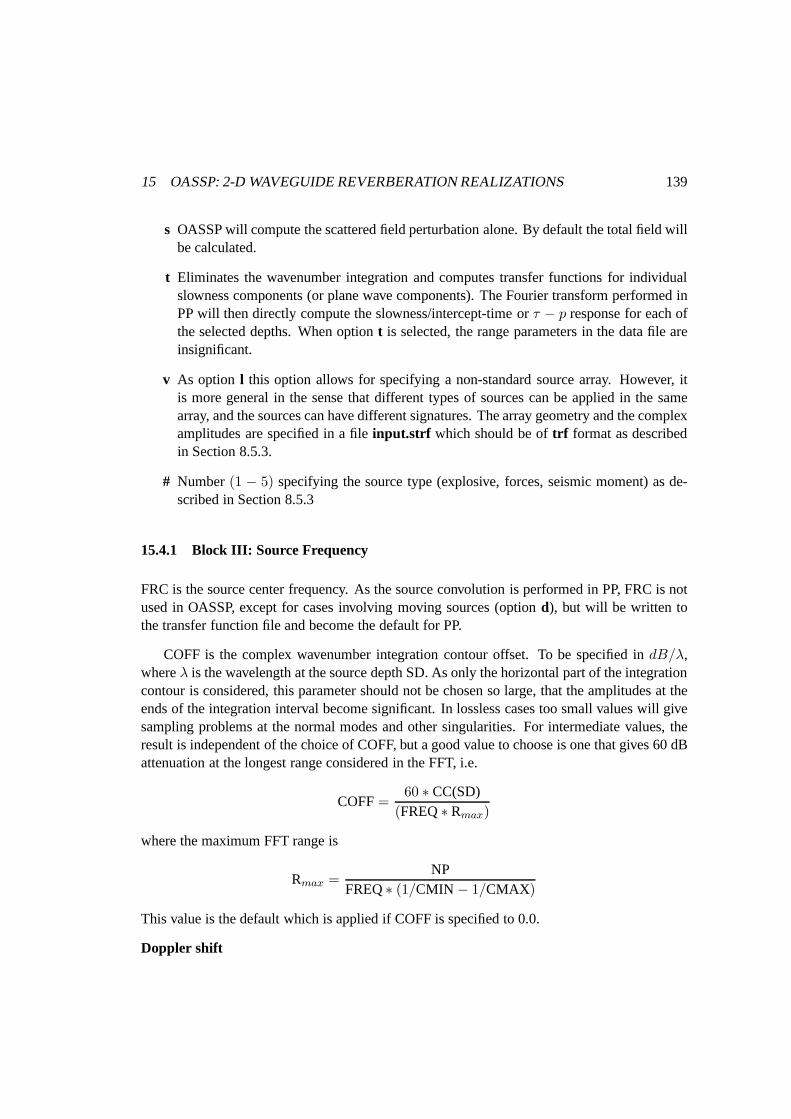
15 OASSP: 2-D WAVEGUIDE REVERBERATION REALIZATIONS 139
s OASSP will compute the scattered field perturbation alone. By default the total field willbe calculated.
t Eliminates the wavenumber integration and computes transfer functions for individualslowness components (or plane wave components). The Fourier transform performed inPP will then directly compute the slowness/intercept-timeor τ − p response for each ofthe selected depths. When optiont is selected, the range parameters in the data file areinsignificant.
v As option l this option allows for specifying a non-standard source array. However, itis more general in the sense that different types of sources can be applied in the samearray, and the sources can have different signatures. The array geometry and the complexamplitudes are specified in a fileinput.strf which should be oftrf format as describedin Section 8.5.3.
# Number(1 − 5) specifying the source type (explosive, forces, seismic moment) as de-scribed in Section 8.5.3
15.4.1 Block III: Source Frequency
FRC is the source center frequency. As the source convolution is performed in PP, FRC is notused in OASSP, except for cases involving moving sources (option d), but will be written tothe transfer function file and become the default for PP.
COFF is the complex wavenumber integration contour offset.To be specified indB/λ,whereλ is the wavelength at the source depth SD. As only the horizontal part of the integrationcontour is considered, this parameter should not be chosen so large, that the amplitudes at theends of the integration interval become significant. In lossless cases too small values will givesampling problems at the normal modes and other singularities. For intermediate values, theresult is independent of the choice of COFF, but a good value to choose is one that gives 60 dBattenuation at the longest range considered in the FFT, i.e.
COFF=60 ∗ CC(SD)
(FREQ∗ Rmax)
where the maximum FFT range is
Rmax =NP
FREQ∗ (1/CMIN − 1/CMAX)
This value is the default which is applied if COFF is specifiedto 0.0.
Doppler shift

15 OASSP: 2-D WAVEGUIDE REVERBERATION REALIZATIONS 140
By specifying optiond in OASP V.1.7 and higher, radialDoppler shift is accounted forusing the theory developed by Schmidt and Kuperman [9]. The source pulse and the radialprojections of the source and receiver velocities must be specified in the input file followingthe specification of the centre frequency and the contour offset (Block II), i.e.
Standard For optiondFRC COFF IT VS VR
IT is a number identifying the source pulse as described in Sec.16. VS andVR are theprojected radial velocities in m/s of the source and receiver, respectively, both being positivein the direction from source to receiver. Since this option requires incorporation of the sourcefunction in the wavenumber integral, the PP post-processormustsubsequently be used withsource pulse -1 (impulse response).
15.4.2 Block IV: Environmental Model
OASSP supports all the environmental models allowed for SAFARI as well as the ones de-scribed above in Section 4.1. The significance of the standard environmental parameters is asfollows
NL: Number of layers, including the upper and lower half-spaces. These should always beincluded, even in cases where they are vacuum.
D: Depth inm of upper boundary of layer or halfspace. The reference depthcan be choosenarbitrarily, and D() is allowed to be negative. For layer no.1, i.e. the upper half-space,this parameter is dummy.
CC: Velocity of compressional waves inm/s. If specified to 0.0, the layer or half-space isvacuum.
CS: Velocity of shear waves in m/s. If specified to 0.0, the layer or half-space is fluid. IfCS()< 0, it is the compressional velocity at bottom of layer, which is treated as fluidwith 1/c(z)2 linear.
AC: Attenuation of compressional waves indB/λ. If the layer is fluid, and AC() is specifiedto 0.0, then an imperical water attenuation is used (Skretting & Leroy).
AS: Attenuation of shear waves indB/λ
RO: Density ing/cm3.
RG: RMS roughness of interface inm. RG(1) is dummy. If RG< 0 it represents the neg-ative of the RMS roughness, and the associated correlation length CL and the spectralexponent should follow. If RG> 0 the correlation length is assumed to be infinite.

15 OASSP: 2-D WAVEGUIDE REVERBERATION REALIZATIONS 141
CL: Roughness correlation length in m. If RG and CL are both negative, the interface isassumed to be smooth, but the layer below will contain volumeinhomogeneities withvertical and horizontal correlation lengths -RG and -CL, respectively.
M: Spectral exponent of the power spectrum as defined by Turgut [25], with 1.5 < M ≤ 2.5for realistic surfaces, with M= 1.5 corresponding to the highest roughness, and M= 2.5being a very smooth variation. For 2-D Goff-Jordan surfaces, the fractal dimension isD = 4.5 − M Insignificant for Gaussian spectrum (optiong not specified) but a valuemust be given.
15.4.3 Volume Scattering Layer
If a volume scattering layer is flagged by RG and CL both being negative, these parameterswill be interpreted as the negative of the vertical and horizontal correlation lengths of the vol-ume inhomogeneities. In this case 4 more parameters should be added on the same line tocompletely describe the spatial statistics:
D CC CS AC AS RO RG CL SKW M RMS GAM
with the significance:
SKW Skewness angle of the correlation ellipse in degrees. 0.0 represents no skewness. Anglemeasured positive downwards.
M Volume spectral exponent as defined by Turgut [25] for power-law spectra. M> 1.5 isrequired for the power spectrum to be integrable, independent on the dimension of theproblem. Insignificant unless optiong was specified.
RMS RMS of relative sound speed perturbation∆c/c for volume inhomogeneities.
GAM Ratioγ of relative density perturbation to sound speed perturbation,∆ρ/ρ = 2.0γ ∆c/c.
15.4.4 Block V: Sources
When computing the total field (options not specified), OASSP supports the same sources asOASP, as described in Sec. 8.5.3, including source arrays. However, the source specificationmust be consistent with the one used for the associated OASP run, since the scattered field iscontrolled by the latter. If options is specified in OASSP, the source type is insignificant.
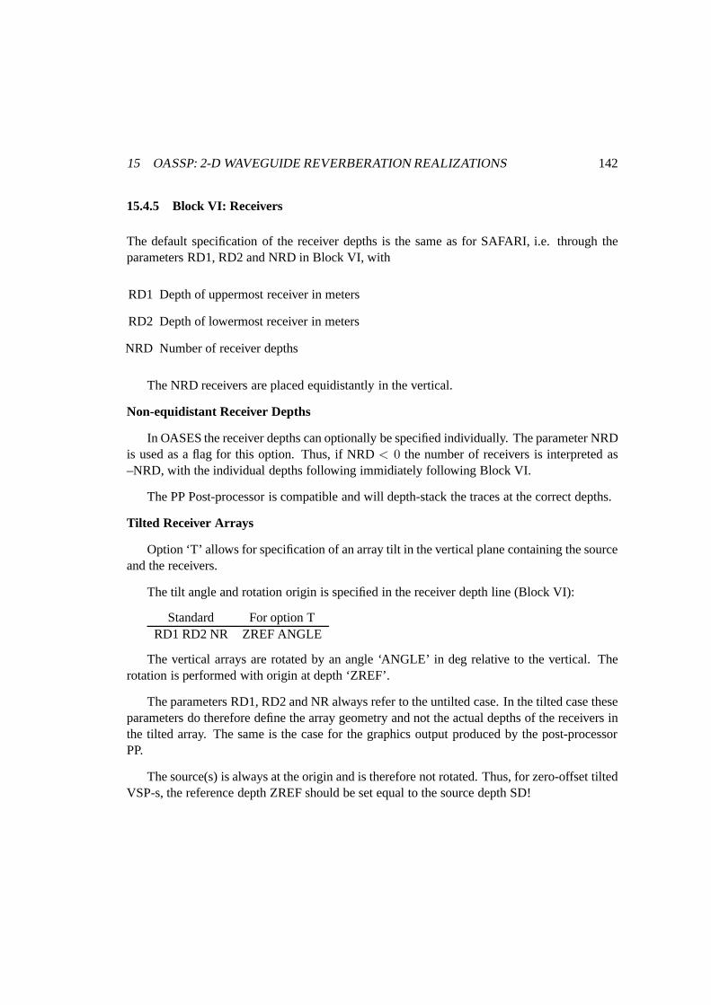
15 OASSP: 2-D WAVEGUIDE REVERBERATION REALIZATIONS 142
15.4.5 Block VI: Receivers
The default specification of the receiver depths is the same as for SAFARI, i.e. through theparameters RD1, RD2 and NRD in Block VI, with
RD1 Depth of uppermost receiver in meters
RD2 Depth of lowermost receiver in meters
NRD Number of receiver depths
The NRD receivers are placed equidistantly in the vertical.
Non-equidistant Receiver Depths
In OASES the receiver depths can optionally be specified individually. The parameter NRDis used as a flag for this option. Thus, if NRD< 0 the number of receivers is interpreted as–NRD, with the individual depths following immidiately following Block VI.
The PP Post-processor is compatible and will depth-stack the traces at the correct depths.
Tilted Receiver Arrays
Option ‘T’ allows for specification of an array tilt in the vertical plane containing the sourceand the receivers.
The tilt angle and rotation origin is specified in the receiver depth line (Block VI):
Standard For option TRD1 RD2 NR ZREF ANGLE
The vertical arrays are rotated by an angle ‘ANGLE’ in deg relative to the vertical. Therotation is performed with origin at depth ‘ZREF’.
The parameters RD1, RD2 and NR always refer to the untilted case. In the tilted case theseparameters do therefore define the array geometry and not theactual depths of the receivers inthe tilted array. The same is the case for the graphics outputproduced by the post-processorPP.
The source(s) is always at the origin and is therefore not rotated. Thus, for zero-offset tiltedVSP-s, the reference depth ZREF should be set equal to the source depth SD!

15 OASSP: 2-D WAVEGUIDE REVERBERATION REALIZATIONS 143
15.4.6 Block VII: Wavenumber integration
This block specifies the wavenumber sampling in the standardOASES format, with the signif-icance of the parameters being as follows:
CMIN: Minimum phase velocity in m/s. Determines the upper limit of the truncated horizontalwavenumber space:
kmax =2π ∗ FREQ
CMIN
CMAX: Maximum phase velocity in m/s. Determines the lower limit of the truncated horizontalwave- number space:
kmin =2π ∗ FREQ
CMAXIn plane geometry ( option P ) CMAX may be specified as negative. In this case, thenegative wavenumber spectrum will be included withkmin = −kmax, yielding correctsolution also at zero range.
NW: Number of sampling points in wavenumber space. In contrast to what is the case forOAST, NW does here not have to be an integer power of 2. The sampling pointsare placed equidistantly in the truncated wavenumber spacedetermined by CMIN andCMAX. If CMAX < 0, i.e. the inclusion of the negative spectrum is enabled, then theNW sample points will be distributed along the positive wavenumber axis only, with thenegative components obtained by symmetry. NW=-1 activatesautomatic wavenumebersampling.
IC1: Number of the first sampling point where the calculationis to be performed. If IC1>1, then the Hankel transform is Hanning-windowed in the interval 1,2. . .IC1-1 beforeintegration. Insignificant for automatic sampling (NW = -1).
IC2: Number of the last sampling point where the calculationis to be performed. If IC2<NWN,then the Hankel transform is Hanning windowed in the interval IC2+1,. . .NW before in-tegration. Insignificant for automatic sampling (NW = -1).
IF: Frequency increment for plotting of integration kernels. A value of 0 disables the plot-ting.
Automatic wavenumber sampling
As foor the other OASES modules the automatic sampling is activated by specifying theparameter NW to−1 and it automatically activates the complex frequency integration contoureven though optionO may not have been specified. The parameters IC1 and IC2 have noeffectif the automatic sampling is selected.

15 OASSP: 2-D WAVEGUIDE REVERBERATION REALIZATIONS 144
15.5 Execution of OASSP
As for the other modules filenames are passed to the code via environmental parameters. InUnix systems a typical command fileoassp(in $HOME/oases/bin) is:
#!/bin/cshsetenv FOR001 $1.dat # input filesetenv FOR002 $1.src # Source array input filesetenv FOR015 $1.strf # Source array trf filesetenv FOR019 $1.plp # plot parameter filesetenv FOR020 $1.plt # plot data filesetenv FOR028 $1.cdr # contour plot parameter filesetenv FOR029 $1.bdr # contour plot data filesetenv FOR045 $2.rhs # mean field amplitudes at rough interf acesetenv FOR046 $2.vol # mean field in volume scattering layeroassp2 # executable
After preparing an OASP data file with the nameinput-rhs.dat , OASP is executedby the command:
> oasp input-rhs
To generate the associated scattered field transfer functions, OASSP is then executed,
> oassp input-scat input-rhs
whereinput-scat.dat is the input file for OASSP.

15 OASSP: 2-D WAVEGUIDE REVERBERATION REALIZATIONS 145
15.6 OASSP - Examples
15.6.1 Rough Seabed Reverberation
This example computes the reverberation in a 200 Hz band around 500 Hz from a rough strat-ified seabed in shallow water. The source is assumed to be a line source (option P). The fieldis computed for vertical arrays at range 0 m (monostatic) and500 m (bistatic). The data filewg-rhs.dat for computing the mean field using automatic sampling is:
Line source. Mean field. Goff. auto.P B N s g O500 040 0 0 0 0 0 00 1500 0 0 0 1 0128. 1470 0000.00 0.01 0.00 1.650 0.5 0228.00 2300 0000.00 0.50 0.00 2.650 0.0000
100.52. 127. 51
1200 -1200-1 1 1 02048 400 600 0.0004 0 .5 2
Figure 5 shows the depth-stacked plots of the the mean field envelopes for the monostaticreceiver array, generated using PP.
The associated input filewg-scat.dat for OASSP is:
Seabed scat. Line source. Goff-J. auto.P B N O s g500 04
0. 0 0 0 0 1 0 00. 1500 0 0 0 1 0 0
128. 1470 0000.00 0.01 0.00 1.650 -0.5 5.0228.00 2300 0000.00 0.50 0.00 2.650 0.0000 0.0
128.77. 127. 51

15 OASSP: 2-D WAVEGUIDE REVERBERATION REALIZATIONS 146
Figure 5: Mean field envelope in shallow water example
1200 -12002048 1 2048 02048 400 600 0.0004 0 0.5 2
The main difference is that the wavenumber sampling was chosen manually here, and a fi-nite roughness correlation length was specified. The field envelopes for the monostatic verticalarray are shown in Fig. 6.
15.6.2 Seabed Volume Scattering
The use of OASSP for computing realizations of scattering and reverberation produced byrandom distributions of volume inhomogeneities in the seabed is illustrated by the followingexample. The environment is similar to the above, but the seasurface is eliminated. The datafile vol-rhs.dat for the OASP mean field is
Halfsp. Line source. Mean field. Goff. auto.P B N s g O500 03128. 1500 0 0 0 1 0 0128. 1470 -2270.10 0.01 0.00 1.650 1.0000 0

15 OASSP: 2-D WAVEGUIDE REVERBERATION REALIZATIONS 147
Figure 6: Reverberant field envelope in shallow water seabedroughness scattering example
228.00 2300 0000.00 0.50 0.00 2.650 0.0000 0
100.77. 127. 51
1200 -1200-1 1 1 02048 400 600 0.0004 0 .5 2
The resulting depth-stacked envelope plot is shown in Fig. 7.
The associated OASSP data filevol-scat.dat for calculating the field scattered is
Volume scat. Line source. . Goff-J. auto.P N s O g500 03128. 1500 0 0 0 1 0 0.0128. 1470 -2270.10 0.01 0.00 1.650 -2.0 -5.0 0 2.5 1.0 0.0228.00 2300 0000.00 0.50 0.00 2.650 0.0000 0.0
128.77. 127. 51

15 OASSP: 2-D WAVEGUIDE REVERBERATION REALIZATIONS 148
Figure 7: Monostatic mean field envelope in shallow water environment with sediment layerhaving a strong sound speed gradient and volume inhomogeneities
1200 -12002048 1 2048 02048 400 600 0.0004 0 0.5 2
With the skewness set to 0 deg the main axes of the correlationfunction are alligned withthe stratification, and the horizontal correlation length is specified to 5 m, with the verticalcorrelation length being 2 m. The fractal dimension of the power law spectrum (option ’g’) is2.5. The RMS relative sound speed perturbation is set to unity, while the relative density is setto 0.
The resulting depth-stacked scattered field envelopes are shown in Fig. 8. The fundamen-tal differences between the scattering from seabed roughness and volume inhomogeneities isdidcussed in Ref. [24].

16 PP - THE OASES PULSE POST-PROCESSOR 149
Figure 8: Monostatic backscattering envelope in shallow water environment with sedimentlayer having a strong sound speed gradient and volume inhomogeneities
16 PP - The OASES Pulse Post-processor
The post-processor PP convolves the transfer functions produced by OASP, RDOASP, OASP3Dor SUPERSNAP with an interactively selected source spectrum and performs the inverse Fouriertransform yielding the synthetics.
The synthetics are plotted directly using MINDIS or PLOTMTV, and a hardcopy can berequested after each plot Alternatively, a trace file can be created in a user specified format,containing the computed timeseries.
16.1 Executing PP
PP is menu-driven, with the menus being machine-independent. The program is executeddirectly without any parameters or switches by issuing the commandpp, prompting with themenu:
*************************************************** ****************** OASES PULSE POST-PROCESSOR **************************************************** ****************** 1. File name: temmllra.trf ** 2. Source type: 2 ( -1 - 6 ) ** 3. Source file: tria.sou *

16 PP - THE OASES PULSE POST-PROCESSOR 150
* 4. Min frequency: 0.000 Hz ** 5. Max frequency: 0.000 Hz ** 6. Cen frequency: 0.000 Hz ** 7. Plot options: SHD,POS ** 8. Contour options:CPX ** 9. Depth stacked: ** 10. Range stacked: ** 11. Azimuth stacked: ** 12. Individual: ** 13. Transmission Los ** 14. Snap shots: ** 15. Source pulses: ** 16. Demodulation: N ( Y/N ) ** 17. Log Traces: N ( Y/N ) ** 18. Save plot files: N ( Y/N ) ** 19. Trace format: A ( Asc/Cfs/Gld/Mat/Sdr ) ** 20. Add TRF files: ** 21. Multiply TRF fil ** 22. Exit PP: **************************************************** *****************
SELECT OPTION: 1File name: ? input.trf
The first option selected is 1 to specify the file name, here a file input.trf containing transferfunctions produced by OASP or another compatible code. PP now reads the header of the fileand displays the frequency interval, the default source type (the source types 1-5 are those givenin the SAFARI manual [4]) and the center frequency specified in the OASP data file. Any ofthese parameters may now be changed if desired. The plot options (field 7) can be specified inthe format described in Sec. 18.1, and similarly for the contour options (field 8) in Sec. 18.2.
16.2 Source Pulses
PP has a set of built-in source pulses, selected in Field 2 of the PP main menu. Types 1 to 5 arethose available in SAFARI [4].
Type 6 is a new pulse type. It is generated as a Hanning windowed sine wave with aduration corresponding to the bandwidth of the transfer function in thetrf -file. This sourcepulse minimizes artificial ringing of the response due to thetruncation of the transfer functionand is the recommended pulse type for narrow band propagation problems.
Type−1 yields the band-limited impulse response by simply eliminating the source pulseconvolution. To reduce truncation ringing the transfer function is Hermite-extrapolated beforebeing Fourier transformed.

16 PP - THE OASES PULSE POST-PROCESSOR 151
Type 0 lets the user input his own pulse shape. The source pulse should be defined in anASCII file in the following format:
t0 p0t1 p1t2 p2t3 p3: :: :tn pn
whereti is the time in seconds andpi is the corresponding source pulse amplitude. The timesampling does not have to be equidistant, and the file needs only contain the actual length ofthe source pulse. PP will use interpolation and zero-padding to conform with the time windowand sampling defined by thetrf -file. The name of the source file is specified in Field 3 of themain menu.
16.3 Trace file format
All timeseries submenues include the option of creating trace files, rather than the scaled plotfiles, for post-processing. A generic ASCII file format is thedefault, while the other formatsrepresent site-specific costumizations. Thus, for example(G chooses the GLD format usedextensively in the past by MIT/WHOI. As the latest addition (Version 2.2 and higher) the tracefiles may be generated directly in MATLAB-5c©format (M ). The matlab util sub-directorycontains a sample MATLAB script,pp matreader.m , for reading the files.
All file formats include a header identifying the traces. Thus, for example, the ASCII filehas a master header with information etc., and a sub-header for each trace with depth, rangeetc. The data for each trace then follow sequencially:
TEMME-MULLER. Auto f.V # Parameter1 # Number of planes
23 # Number of traces1001 # Number of samples/trace
1000.00 # Sampling frequency in Hz
600.000 # Range (m)50.0000 # Depth (m)
0.000000E+00 # Bearing (deg)0.000000E+00 # Starting time (sec)
-0.366703E-08 -0.292363E-08 -0.200186E-08 -0.977132E-0 9 0.445733E-100.947549E-09 0.163239E-08 0.203979E-08 0.216378E-08 0.2 05015E-08

16 PP - THE OASES PULSE POST-PROCESSOR 152
.
.0.253403E-06 0.303194E-06 0.327134E-06 0.318899E-06 0.2 78182E-060.211619E-06
600.000 # Range (m)75.0000 # Depth (m)
0.000000E+00 # Bearing (deg)0.000000E+00 # Starting time (sec)0.371295E-08 0.323503E-08 0.249180E-08 0.154489E-08 0.4 74728E-09
.
.
Field 16 and 17 control the plot format for all timeseries plots and trace outputs. IF ’Y’is selected in field 16, all timeseries will be demodulated bythe centre frequency to generatethe magnitude complex signal envelope. If in addition ’Log traces’ is chosen in field 17, themagnitude envelopes will be plotted or output in dB. This option is particularly useful whenlarge dynamic range is needed, such as for reverberation simulations using OASSP.

16 PP - THE OASES PULSE POST-PROCESSOR 153
16.4 Depth-Stacked Time Series
If the synthetics should be depth-stacked, Field 9 is selected in the main menu, showing thesub-menu:
*************************************************** ******************* DEPTH STACKED PLOTS **************************************************** ******************* 1. Plot title: TEMME-MULLER. Auto f. ** 2. Min time: 0.000 s ** 3. Max time: 1.000 s ** 4. Time tick inc: 0.200 s ** 5. t-axis length: 20.000 cm ** 6. Depth down: 700.000 m ** 7. Depth up: 0.000 m ** 8. Depth tick inc: 100.000 m ** 9. d-axis length: 15.000 cm ** 10. d-axis label: Depth (m) ** 11. Red. velocity: 0.000 m/s ** 12. Range: 0.600 km ** 13. Azimuth: 0.000 deg ** 14. Scale factor: 1.000 ** 15. Parameter: V ( V H ) ** 16. Generate plot: ** 17. Trace file: ** 18. Return: ( PP main menu ) **************************************************** ******************
SELECT OPTION:
The menu should be self explanatory for users familiar with SAFARI, with only the fol-lowing being particular to PP:
Field 12 selects the receiver range.
Field 13 specifies the azimuth of the receiver plane. This parameter is only significant fortransfer functions with horizontal directionality, produced by OASP3D.
Field 14 represents a scaling factor which will be applied to all traces. The default is 1.0, i.e.no scaling, but may be changes as desired.
Field 15 represents the parameter to be plotted, consistent with theoptions specified in theOASP data file, i.e. with N representing the normal stress or negative pressure in fluids,V the vertical particle velocity and H the horizontal particle velocity etc. The bracketindicates that only V and H transfer functions are availablein the file, and the programwill therefore not allow any other choice.

16 PP - THE OASES PULSE POST-PROCESSOR 154
Field 16 produces the plot with the specified parameters.
Field 17 produces a trace file containing the time series, in file format specified in main menu(default ASCII). The trace file include all the timeseries which would be included in thestacked plot.
Field 18 Returns to main menu for change of e.g. source data, plot format etc.

16 PP - THE OASES PULSE POST-PROCESSOR 155
16.5 Range-Stacked Time Series
If instead the range stacking was selected the following menu appears:
*************************************************** ******************* RANGE STACKED PLOTS **************************************************** ******************* 1. Plot title: TEMME-MULLER. Auto f. ** 2. Min time: 0.000 s ** 3. Max time: 1.000 s ** 4. Time tick inc: 0.200 s ** 5. T-axis length: 20.000 cm ** 6. Range down: -0.500 km ** 7. Range up: 1.000 km ** 8. Range tick inc: 0.500 km ** 9. R-axis length: 15.000 cm ** 10. R-axis label: Range (km) ** 11. Red. velocity: 0.000 m/s ** 12. Depth: 600.000 m ** 13. Azimuth: 0.000 deg ** 14. Scale factor: 1.000 ** 15. Range scaling? N ( Y/N ) ** 16. Parameter: V ( V H ) ** 17. Generate plot: ** 18. Trace file: ** 19. Return: ( PP main menu ) **************************************************** ******************
SELECT OPTION:
The menu should be self explanatory for users familiar with SAFARI, with only the followingbeing particular to PP:
Field 12 selcts the depth of the receivers to be stacked.
Field 13 specifies the azimuth of the receiver plane. This parameter is only significant fortransfer functions with horizontal directionality, produced by OASP3D.
Field 14 represents a scaling factor which will be applied to all traces. The default is 1.0, i.e.no scaling, but may be changes as desired.
Field 15 enables/disables the range scaling (amplitudes multiplied by range). By defaultsrange scaling is enabled.
Field 16 represents the parameter to be plotted, with N representingthe normal stress or neg-ative pressure in fluids, V the vertical particle velocity and H the horizontal particle

16 PP - THE OASES PULSE POST-PROCESSOR 156
velocity. The bracket indicates that only V and H transfer functions are available in thefile, and the program will therefore not allow any other choice.
Field 17 produces the plot with the specified parameters.
Field 18 produces a trace file containing the time series, in file format specified in main menu(default ASCII). The trace file include all the timeseries which would be included in thestacked plot.
Field 19 Returns to main menu for change of e.g. source data, plot format etc.

16 PP - THE OASES PULSE POST-PROCESSOR 157
16.6 Azimuth-Stacked Time Series
If the azimuth stacking was selected the following menu appears:
*************************************************** ******************* AZIMUTH STACKED PLOTS **************************************************** ******************* 1. Plot title: TEMME-MULLER. Auto f. ** 2. Min time: 0.000 s ** 3. Max time: 1.000 s ** 4. Time tick inc: 0.200 s ** 5. t-axis length: 20.000 cm ** 6. Azimuth down: -50.000 deg ** 7. Azimuth up: 400.000 deg ** 8. Azim. tick inc: 50.000 deg ** 9. a-axis length: 15.000 cm ** 10. Red. velocity: 0.000 m/s ** 11. Range: 0.600 km ** 12. Depth: 600.000 m ** 13. No. of traces: 18 ( 1 - 999 ) ** 14. Scale factor: 1.000 ** 15. Parameter: V ( V H ) ** 16. Generate plot: ** 17. Trace file: ** 18. Return: ( PP main menu ) **************************************************** ******************
SELECT OPTION:
The menu should be self explanatory for users familiar with SAFARI, with only the followingbeing particular to PP:
Field 11 specifies the range of the receivers in km.
Field 12 specifies the depth of the receivers in meters.
Field 13 specifies the number of azimuths of the receiver plane for which the response shouldbe computed and stacked.
Field 14 represents a scaling factor which will be applied to all traces. The default is 1.0, i.e.no scaling, but may be changes as desired.
Field 15 represents the parameter to be plotted, with N representingthe normal stress or neg-ative pressure in fluids, V the vertical particle velocity and H the horizontal particlevelocity. The bracket indicates that only V and H functions are available in the file, andthe program will therefore not allow for any other choice.

16 PP - THE OASES PULSE POST-PROCESSOR 158
Field 16 produces the plot with the specified parameters.
Field 17 produces a trace file containing the time series, in file format specified in main menu(default ASCII). The trace file include all the timeseries which would be included in thestacked plot.
Field 19 Returns to main menu for change of e.g. source data, plot format etc.

16 PP - THE OASES PULSE POST-PROCESSOR 159
16.7 Transmission Loss Plots
Version 2.1 of PP has been modified to allow for plotting of transmission losses, derived fromthe OASP transfer functions. This also allows for extreme near-field transmission loss compu-tations with the full exact Bessel function integration (OASP optionf).
Choosing field 13 brings up the transmission loss submenu,, allowing selction of plot for-mats, currently supporting TL vs range, depth or frequency,depth-averaged TL, or depth-rangecontours:
*************************************************** ****************** TRANSMISSION LOSS **************************************************** ****************** 1. TL vs Freq: ** 2. TL vs Range: ** 3. TL vs Depth: ** 4. Depth Average: ** 5. Depth-Range Cont ** 6. Return: ( PP main menu ) **************************************************** *****************
SELECT OPTION: 5--------------------
*************************************************** ****************** DEPTH-RANGE TL CONTOURS **************************************************** ****************** 1. Plot title: TEMME-MULLER. Auto f. ** 2. Range left: 0.000 km ** 3. Range right: 0.600 km ** 4. Range tick inc: 0.100 km ** 5. R-axis length: 20.000 cm ** 6. Depth down: 600.000 m ** 7. Depth up: 0.000 m ** 8. Depth tick inc: 100.000 m ** 9. D-axis length: 12.000 cm ** 10. Azimuth: 0.000 deg ** 11. Frequency: 50.000 Hz ** 12. Min. loss: 30.000 dB ** 13. Max. loss: 90.000 dB ** 14. Increment: 3.000 dB ** 15. Undef. file: ** 16. Shade file: ** 17. Parameter: V ( V H ) ** 18. Generate plot: ** 19. Return: ( PP main menu ) **************************************************** *****************
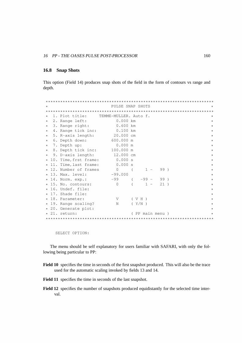
16 PP - THE OASES PULSE POST-PROCESSOR 160
16.8 Snap Shots
This option (Field 14) produces snap shots of the field in the form of contours vs range anddepth.
*************************************************** ******************* PULSE SNAP SHOTS **************************************************** ******************* 1. Plot title: TEMME-MULLER. Auto f. ** 2. Range left: 0.000 km ** 3. Range right: 0.600 km ** 4. Range tick inc: 0.100 km ** 5. R-axis length: 20.000 cm ** 6. Depth down: 600.000 m ** 7. Depth up: 0.000 m ** 8. Depth tick inc: 100.000 m ** 9. D-axis length: 12.000 cm ** 10. Time,frst frame: 0.000 s ** 11. Time,last frame: 0.000 s ** 12. Number of frames 0 ( 1 - 99 ) ** 13. Max. level: -99.000 ** 14. Norm. exp.: -99 ( -99 - 99 ) ** 15. No. contours: 0 ( 1 - 21 ) ** 16. Undef. file: ** 17. Shade file: ** 18. Parameter: V ( V H ) ** 19. Range scaling? N ( Y/N ) ** 20. Generate plot: ** 21. return: ( PP main menu ) **************************************************** ******************
SELECT OPTION:
The menu should be self explanatory for users familiar with SAFARI, with only the fol-lowing being particular to PP:
Field 10 specifies the time in seconds of the first snapshot produced. This will also be the traceused for the automatic scaling invoked by fields 13 and 14.
Field 11 specifies the time in seconds of the last snapshot.
Field 12 specifies the number of snapshots produced equidistantly for the selected time inter-val.

17 INTERFACE TO MATLAB POST PROCESSING 161
Field 13 Is used to set the maximum levelAmaxfor the contours. The interval[−Amax, Amax]will be equidistantly covered by the number of contours specified in Field 13.
Field 14 Here the logarithm of the scaling factor is specified. If -99 is specified the exponentwill be selected automatically based on the snap-shot data.Usually the first snap-shotis made with automatic scaling, whereas the rest are produced with the so determinedexponent. The automatic scaling will also suggest a value ofAmax in Field 11, whichmay of course be changed by the user if desired.
Field 15 Number of contour levels applied for snapshots. For UNIRAS colour plots this num-ber should not be more that 12. UNIRAS is selected by specifying the contour optionsUNI,X11,COL in Field 8 of the main menu (X11 selects X-windows as device).
Field 16 Name of a file containing a binary map of undefined points.
Field 17 Name of file containing the coordinates of an optional shadedpolygon superimposedto the snap-shot. Used for shading bottom or objects. The fileformat is the standardshading specification used in thecdr files providing plot parameters tocplot.
Field 18 represents the parameter to be plotted, consistent with theoptions specified in theOASP data file, i.e. with N representing the normal stress or negative pressure in fluids,V the vertical particle velocity and H the horizontal particle velocity etc.
Field 19 a ’Y’ here applies a linear scaling of the snapshots with horizontal range, similar tothe range scaling in the range-stacked plots. This is usefulfor animations of near-fieldproblems with significant geometric spreading.
Field 20 produces the contour plots with the specified parameters.
Field 21 Returns to main menu for change of e.g. source data, plot format etc.
17 Interface to MATLAB Post Processing
An alternative to using the PP postprocessor for generatinggraphics, producing timeseries etc.,is to use MATLAB. A number of matlab utilities for producing high quality graphics and forprocessing the simulated transfer functions and timeseries has been developed by OASES usersover the years. A collection of very powerful and well documented set of utilities are includedin the OASES distribution, in the directoryOases/matlab util/ .
17.1 Reading Transfer Function Files
The scripttrf reader oases3d.m reads the binary transfer function files( * .trf) intoMATLAB. The use of this and other scripts inmatlab util is described in the header of

17 INTERFACE TO MATLAB POST PROCESSING 162
the script, visualized using the MATLABhelp command,
>> help trf_reader_oases3Dfunction[out,sd,z,range,f,fo,omegim,msuft]=trf_read er_oases3d(fname)
function to read oases trf file and return contents
Kevin D. LePageSACLANTCEN22/8/00
INPUTS
fname file name (ascii string, with our without .trf extensi on)
OUTPUTS
out complex transfer function (length(z)xlength(r)xleng th(f))sd source depth (m)z receiver depthsrange receiver rangesf receiver frequenciesfo receiver center frequencyomegim imaginary part of radian frequencymsuft number of Fourier harmonics
>>
Thus, for example, for the synthetic sesmogram example inOases/pulse , use thecommands,
> cd Oases/pulse> oasp temmllr> matlab
>>[out,sd,z,range,f,fo,omegim,msuft]=trf_reader_oases 3d(’temmllr.trf’);
>> here goes your own processing stuff

17 INTERFACE TO MATLAB POST PROCESSING 163
17.2 Reading PP Timeseries Files
Another MATLAB interface is a script, which reads the.mat files optionally generated byPP,
help pp_matreader[ts,t,z,r,b,tit,parameter,planes,traces,samples,fs] =pp_matreader(file)
function to read mat files output by pp
Eddie ScheerWHOI8/24/99
INPUTS
file file name (string)
OUTPUTS
ts time series (length(t) x (planes x traces))t start timesz depths (vector of corresponding depths)r range (vector of corrsponding ranges)b bearing (vector of corresponding bearings)title character stringparameter character string (N is normal stress)planes number (for different bearings, for instance)traces number (for depth or range stacks, for instance)samples number (N)fs sample frequency (Hz)
>>

18 GRAPHICS POST-PROCESSORS 164
18 Graphics Post-Processors
18.1 mplot
mplot is one of the graphics post-processors used in connection with OASES and other com-patible acoustic propagation models. It produces publication quality line-style graphics usingtheMINDIS graphics library.
Alternatively, plotmtv may be chosen as the default line plot package by setting anenvironment variable:
setenv PLP_PACKGE MTV
It should be noted that some of themplot options described below may not be fullysupported byplotmtv.
18.1.1 Input files
mplot requires two input files, with extensionsplp andplt .
The file with extensionplp contains plot parameters such as axis lengths, titles, labelsetc, whereas the other file, with extensionplt , contains the actual data values to be plotted.Both files are formatted ASCII files, and it is therefore possible to change the layout of theplots by editing theplp file.
A typical plp file is:
1024 MODULO_FIPP__STLDAV,CPX,IYA_DEPTH AVERAGED LOSS_SAFARI-FIP case 3._ 2 NUMBER OF LABELS_Freq: 30.0 Hz$_SD: 50.0 m$_ 20.000000 XLEN_ 12.000000 YLEN_ 0 GRID TYPE_ 0.000000 XLEFT_ 5.00000 XRIGHT_ 1.00000 XINC_ 1.00000 XDIV_Range (km)$
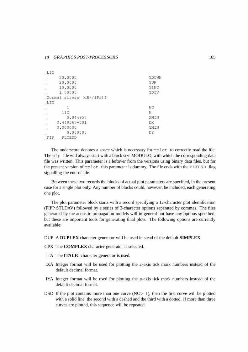
18 GRAPHICS POST-PROCESSORS 165
_LIN_ 80.0000 YDOWN_ 20.0000 YUP_ 10.0000 YINC_ 1.00000 YDIV_Normal stress (dB//1Pa)$_LIN_ 1 NC_ 112 N_ 0.044957 XMIN_ 0.449567-001 DX_ 0.000000 YMIN_ 0.000000 DY_FIP___PLTEND
The underscore denotes a space which is necessary formplot to correctly read the file.Theplp file will always start with a block size MODULO, with which thecorresponding datafile was written. This parameter is a leftover from the versions using binary data files, but forthe present version ofmplot this parameter is dummy. The file ends with thePLTEND flagsignalling the end-of-file.
Between these two records the blocks of actual plot parameters are specified, in the presentcase for a single plot only. Any number of blocks could, however, be included, each generatingone plot.
The plot parameter block starts with a record specifying a 12-character plot identification(FIPP STLDAV) followed by a series of 3-character options separated by commas. The filesgenerated by the acoustic propagation models will in general not have any options specified,but these are important tools for generating final plots. Thefollowing options are currentlyavailable:
DUP A DUPLEX character generator will be used in stead of the defaultSIMPLEX .
CPX TheCOMPLEX character generator is selected.
ITA The ITALIC character generator is used.
IXA Integer format will be used for plotting thex-axis tick mark numbers instead of thedefault decimal format.
IYA Integer format will be used for plotting they-axis tick mark numbers instead of thedefault decimal format.
DSD If the plot contains more than one curve (NC> 1), then the first curve will be plottedwith a solid line, the second with a dashed and the third with adotted. If more than threecurves are plotted, this sequence will be repeated.

18 GRAPHICS POST-PROCESSORS 166
COL This option will plot individual curves in different colour, using the repeatable sequence:red - green - blue - cyan - magenta - yellow. Also affects the shading optionSHD .
MRK A marker will be plotted for each 10th data point on the curves. In the case of morecurves, different markers will be used for each.
TCT This option is used in connection with the stacked time series plots in order to truncatethe amplitude of each trace at an amplitude corresponding tohalf the distance betweentraces.
SHD Produces shaded wiggles on timeseries plots. If specified alone both positive and neg-ative wiggles will be shaded. If specified together with optionsPOS or NEG only thepositive or negative wiggles will be shaded, respectively.If specified together withCOLthe shading is color coded depending on the amplitude. Currently the shading will onlyappear on the hardcopy devices.
POS Shading only applied to positive wiggles.
NEG Shading only applied to negative wiggles.
NWR Disables plotting of the option at the upper right cornerof the plot. Used when generatingfinal figures for documents.
NOP This option will read both the parameters from theplp file and the data from thepltfile but no plot is produced. It is therefore used for time saving when only selected plotsare required.
The next record specifies the main title of the plot, followedby a record containing the titlespecified in the data file for the propagation models. This title will be plotted just above theplot frame.
There is then a sub-block containing the labels to be plottedin the upper right corner of theplot frame. The number of labels (≥ 0) is given first, followed by the label texts, each of whichshould be on separate lines and terminated by a $.
The parameters XLEN and YLEN specify the length in cm of thex- andy-axis, respec-tively. The parameter labelledGRID TYPE indicates whether a grid should be plotted. Avalue of 1 will produce a dotted grid.
The next 6 records contain the parameters for thex-axis of the plot.XLEFT andXRIGHTare the data values at the left and right borders of the plot frame, respectively, whereasXINCis the distance in the same units between the tick marks.XDIV is a multiplication factorwhich will be applied to both the axis parameters and the datavalues. AfterXDIV thex-axislabel is specified, terminated by a $, and finallyLIN indicates that thex-axis should be linear.

18 GRAPHICS POST-PROCESSORS 167
Another possibility is a logarithmic axis, which has not yetbeen implemented however. Theparameters for they-axis are given in the same way in the next 6 records.
The parameterNC specifies the number of curves to be plotted. For each curve a sub-block of 5 records has to be specified. The first parameterN indicates the number of pointsin the curve. IfN is negative, no curve will be plotted; instead a marker will be plotted atthe position of each data point. The parameterXMIN is thex-coordinate (range) of the firstdata point, whereasDX is the equidistant spacing. IfDX had been specified as 0, then theNx-coordinates of the data points would be read from theplt file. In that caseXMIN wouldbe interpreted as anx-offset to be applied to the curve. The same rules apply toYMIN andDY. In the above example they-values will therefore be read from the PLT file, and noy-offsetwill be applied. The offsets are mainly used for the stacked time series plots If bothDX andDY are specified as 0, thenmplot will first read allN x-values and then ally-values.
18.1.2 Executing mplot
To executemplot , prepare the input files, e.g.input.plp andinput.plt as describedabove. Then execute the script
mplot input
18.2 cplot
cplot is the standard script for producing contour plots generated by SAFARI, OASES orSNAP. However,cplot is available for more general use, provided the data to be contouredand the plot lay-out parameters are file-structured as described below.
The plot lay-out parameters are transferred tocplot in a file with extension.cdr ,whereas the actual contour data are transferred in a file withextension.bdr . The data file isallowed to be in both ASCII or binary format, but in computational environments with differenttypes of hardware platforms, it is most convenient to use ASCII format.
Thecdr file can be edited for changing the layout of the contour plot.As a typical exam-ple, thecdr file used to create the contour plot in Fig. 14b of theSAFARI User’s Guideis asfollows:
CONDR,FIP,FMT,CPX,UNI,TEKSAFARI-FIP case 5.saffip5.bdrRange (m)
0.0000 RMIN

18 GRAPHICS POST-PROCESSORS 168
299.8535 RMAX0.0000 XLEFT
300.0000 XRIGHT15.0000 XSCALE50.0000 XINC
Depth (m)50.0000 YUP
125.0000 YDOWN6.2500 YSCALE
25.0000 YINC141.0000 DATA POINTS ALONG X AXIS
51.0000 DATA POINTS ALONG Y AXIS1.0000 DIVX1.0000 DIVY0.0000 FLAGRC
50.0000 RDUP125.0000 RDLO
50.0000 SOURCE DEPTH (M)141.0000 GRID POINTS ALONG X AXIS
51.0000 GRID POINTS ALONG Y AXIS1000.0000 FREQUENCY (HZ)
0.0000 DUMMY5.0000 CAY5.0000 NRNG
21.0000 ZMIN54.0000 ZMAX
3.0000 ZINC2.0000 X ORIGIN OF PLOT IN INCHES0.0000 DUMMY2.0000 Y ORIGIN OF PLOT IN INCHES0.0000 NSM0.1000 HGTPT0.1400 HGTC
-3.0000 LABPT1.0000 NDIV5.0000 NARC
-1.0000 LABC-1.0000 LWGT
BOTTOM 10.0 100.0
300.0 100.0300.0 120.0
0.0 120.0BOTTOM 3
0.0 120.0300.0 120.0300.0 125.0

18 GRAPHICS POST-PROCESSORS 169
0.0 125.0
The first record specifies one 5-character option (CONDR) followed by a series of 3-letteroptions. The CONDR option indicates that the actual contourplot is of the depth-range typeandcplot will interpret the parameters accordingly.This option should therefore never bechanged. The first 3-letter option (FIP) is purely for identificationand has no further effect.The FMT option indicates that thebdr data file is ASCII formatted (BIN for binary format).These first 3 options should always be present in the specifiedorder, but the options followingare optional and can be given in any order. The implemented options are as follows:
DUP TheDUPLEX character generator will be used for MINDIS plots instead ofthe defaultSIMPLEX .
CPX TheCOMPLEX character generator is selected for MINDIS plots.
ITA The ITALIC character generator will be used by MINDIS.
MIN The MINDIS plot package will be used to produce line contour plots.
MTV The PLOTMTV plot package will be used to generate a colouror greytone contour plot.MINDIS is the default plot package.
UNI The UNIRAS plot package will be used to generate a colour or greytone contour plot.MINDIS is the default plot package.
X11 The raster plot will be produced on the X-windows displaydefined by the current settingof theDISPLAY environmental variable. (UNIRAS only).
TEK The raster plot will be produced on the Tektronix 4691 inkjet plotter (UNIRAS only).
LAS The raster plot will be produced on the default laser printer (UNIRAS only).
CLA A Colour-Postscript file is created which may be printed on a colour laser printer (UNI-RAS only).
PSP A Grey-tone Postscript file in portrait mode is created for later printing or inclusion inLaTeX documents.
PSL A Grey-tone Postscript file in landscape mode is created for later printing or inclusion inLaTeX documents.
COL If the options MTV or UNI has been selected, a colour raster plot using an inbuilt colourscale will be generated. By default greytone scale is applied (UNIRAS and PLOTMTV).
REV Reverses the default colour or grey-tone scales (UNIRASonly).

18 GRAPHICS POST-PROCESSORS 170
ROT UNIRAS plots will be rotated 90 degrees. On most graphicsdevices the default is land-scape mode.
NCL By default the raster plots will have the contour lines separating the levels plotted aswell. This option disables this feature.
NCS By default a colour scale will be produced to the right of the contour map. This optiondisables this feature.
If you are usingcplot through X-Windows, UNIRAS or PLOTMTV plots may alter-natively be generated interactively after the default MINDIS plot is produced. The defaultgraphics package may be changed by setting environmental parameters. Thus, to change thedefault to PLOTMTV color in X-windows, use the following definitions in your.login file:
setenv CON_BWCOL COLsetenv CON_PACKGE MTVsetenv CON_DEVICE X11
PLOTMTV is available in public domain, and is easily installed, as described inSection 2.3.
After the option record there is a record containing the title of the plot and a record contain-ing the name of the file containing the data, i.e. thebdr file. Except for 2 records containingthex-axis andy-axis labels, the rest of the records contain numerical parameters, all suppliedwith a descriptive label. In general only a few of these parameters should be changed. Themost important ones are described below.
The lengths of thex- andy-axes are controlled by the parameters XSCALE and YSCALE,respectively. cplot requires these parameters to be specified in coordinate units per cm.ZMIN and ZMAX specify the limits of the contouring interval,whereas ZINC is the associatedincrement. If UNIRAS is selected, areas with small data values will be filled with magentacolour or black in the greytone mode. The colour scale then moves through different red tonesinto blue (white in the greytone mode). If the default MINDISpackage is selected, only contourlines with identifying numbers are plotted.
Another important parameter is NSM, which controls the amount of smoothing appliedto the calculated contours. This parameter can be set to any value between 0 and 10, with 0corresponding to no smoothing. It is obvious that this parameter should be used with extremecare.
At the end of the file, any number of blocks – identified by the keyword BOTTOM– canbe specified, creating a shaded polygon in one of 4 grey-tonesas specified by the numberfollowing the keywordBOTTOM(1 is light grey and 4 black). Each line following states thex- andy-coordinates of the corners of the polygon.
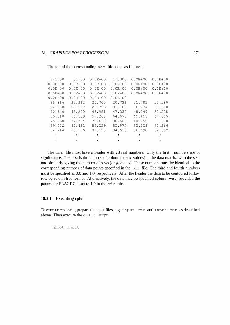
18 GRAPHICS POST-PROCESSORS 171
The top of the correspondingbdr file looks as follows:
141.00 51.00 0.0E+00 1.0000 0.0E+00 0.0E+000.0E+00 0.0E+00 0.0E+00 0.0E+00 0.0E+00 0.0E+000.0E+00 0.0E+00 0.0E+00 0.0E+00 0.0E+00 0.0E+000.0E+00 0.0E+00 0.0E+00 0.0E+00 0.0E+00 0.0E+000.0E+00 0.0E+00 0.0E+00 0.0E+00
25.866 22.212 20.700 20.726 21.781 23.28024.908 26.937 29.723 33.102 36.234 38.50040.540 43.220 45.981 47.238 48.749 52.22555.318 56.159 59.268 64.670 65.453 67.81575.660 77.704 79.630 90.666 109.52 91.88889.072 87.422 83.239 85.975 85.229 81.26684.744 85.196 81.190 84.615 86.690 82.392
: : : : : :: : : : : :
The bdr file must have a header with 28 real numbers. Only the first 4 numbers are ofsignificance. The first is the number of columns (orx-values) in the data matrix, with the sec-ond similarly giving the number of rows (ory-values). These numbers must be identical to thecorresponding number of data points specified in thecdr file. The third and fourth numbersmust be specified as 0.0 and 1.0, respectively. After the header the data to be contoured followrow by row in free format. Alternatively, the data may be specified column-wise, provided theparameter FLAGRC is set to 1.0 in thecdr file.
18.2.1 Executing cplot
To executecplot , prepare the input files, e.g.input.cdr andinput.bdr as describedabove. Then execute thecplot script
cplot input

REFERENCES 172
References
[1] H. Schmidt and F.B. Jensen. A full wave solution for propagation in multilayered vis-coelastic media with application to Gaussian beam reflection at fluid-solid interfaces.J.Acoust. Soc. Am., 77:813–825, 1985.
[2] H. Schmidt and G. Tango. Efficient global matrix approachto the computation of syntheticseismograms.Geophys. J. R. Astr. Soc., 84:331–359, 1986.
[3] F.B. Jensen, W.A. Kuperman, M.B. Porter, and H. Schmidt.Computational Ocean Acous-tics. American Institute of Physics, New York, 1994.
[4] H. Schmidt. SAFARI: Seismo-acoustic fast field algorithm for range independent environ-ments. user’s guide. SR 113, SACLANT ASW Research Centre, LaSpezia, Italy, 1987.
[5] M. Stern, A. bedford and H.R. Millwater. Wave reflection from a sediment layer withdepth-dependent properties.j. Acoust.Soc. Am., 77:1781–1788, 1985.
[6] J.M. Hovem and J.D. Ingram. Viscous attenuation of soundin saturated sand.J. Acoust.Soc. Am., 66:1807–1812, 1979.
[7] B. Yavari and A. Bedford. Comparison of numerical calculations of two Biot coefficientswith analytical solutions.J. Acoust. Soc. Am., 90:985–990, 1991.
[8] M.A. Biot. Theory of propagation of elastic waves in a fluid saturated porous solid.J.Acoust. Soc. Am., 28:168–191, 1956.
[9] H. Schmidt and W.A. Kuperman, Spectral and modal representations of the Doppler-shifted field in ocean waveguides,J. Acoust. Soc. Am., 96(1):386–395, 1994.
[10] J.S. Kim. Radiation from directional seismic sources in laterally stratified media withapplication to Arctic ice cracking noise. PhD thesis, Massachusetts Institute of Technology,May 1989.
[11] H. Schmidt and J. Glattetre. A fast field model for three-dimensional wave propagation instratified environments based on the global matrix method.J. Acoust. Soc. Am., 78:2105–2114, 1985.
[12] H. Schmidt and W.A. Kuperman. Estimation of surface noise source level from low-frequency seismoacoustic ambient noise measurements.J. Acoust. Soc. Am., 84:2153–2162, 1988.
[13] A.B. Baggeroer, W.A. Kuperman and H. Schmidt. Matched field processing: Sourcelocalization in correlated noise as an optimum parameter estimation problem.J. Acoust.Soc. Am., 83:571–587, 1988.

REFERENCES 173
[14] H. Schmidt, A.B. Baggeroer, W.A. Kuperman and E.K. Scheer. Environmentally tolerantbeamforming for high-resolution matched field processing:deterministic mismatch.J.Acoust. Soc. Am., 88:1851–1862, 1990.
[15] H. Schmidt and W.A. Kuperman. Spectral representations of rough interface reverberationin stratified ocean waveguides,J. Acoust. Soc. Am., 96:Submitted, 1994.
[16] W.A. Kuperman and H. Schmidt, Self-consistent perturbation approach to rough surfacescattering in stratified elastic media,J. Acoust. Soc. Am., 86:1511–1522, 1989.
[17] A.B.Baggeroer and H. Schmidt, “Parameter estimation bounds and the accuracy of fullfield inversions.” In O. Diachok, et al, editor,Full field inversion methods in ocean andseismic acoustics, Kluwer Academic Publishers, Dordrecht, The Netherlands,1994.
[18] H. Schmidt and A.B.Baggeroer. “Physics-imposed resolution and robustness issues inseismo-acoustic parameter inversion”. In O.Diachok, et al, editor,Full field inversion meth-ods in ocean and seismic acoustics, Kluwer Academic Publishers, Dordrecht, The Nether-lands, 1994.
[19] H. Schmidt, W. Seong, and J.T. Goh, “Spectral super-element approach to range-dependent ocean acoustic modeling,”J. Acoust. Soc. Am., 98(1), 465–472, 1995.
[20] J.T. Goh and H. Schmidt, A hybrid coupled wavenumber integration approach to range-dependent seismo-acoustic modeling, J. Acoust. Soc. Am, 100, 1409–1420, 1996.
[21] J.T. Goh, H. Schmidt, P. Gerstoft and W. Seong, “Benchmarks for validating range-dependent seismo-acoustic propagation codes”, IEEE J. Oceanic Eng., April 1997.
[22] R.D. Stoll and T.K. Kan, “Reflection of acoustic waves ata water sediment interface,” J.Acoust. Soc. Am., 70, 149–156, 1981.
[23] H. Schmidt and A.B. Baggeroer, ”Physics-imposed resolution and robustness issues inseismo-acoustic parameter inversion”, In ”O. Diachoket al. Eds.” Full field inversionmethods in ocean and seismic acoustics, Kluwer Academic Publishers, Dordrecht, TheNetherlands, 1994.
[24] K. Lepage and H. Schmidt, ”Spectral integral representations of scattering from volumeinhomogeneities in ocean waveguides”, Submitted to J. Acoust. Soc. Am., June 1999.
[25] A. Turgut, “Inversion of bottom/subbottom statistical parameters from acoustic backscat-ter data”, J. Acoust. Soc. Am., 102(2), 833–852, 1997.

A POROUS MEDIA MODEL 174
A Porous Media Model
The Model
The equations of motion for a porous sediment layer may be written in the form[5]
µ∇2u+ (H − µ)∇e− C∇ζ = ρu− ρf w
C∇e−M∇ζ = ρf u−cmρfφ
w −Fη
κw
whereu is the displacement vector associated with the frame andw = φ(u − uf ) is theweighted (by porosity) relative displacement of the frame with respect to the pore fluid. Alsoe = divu andζ = divw; ρ = φρf +(1−φ)ρs is the average density of the saturated sedimentandH, C, andM are (complex) elastic moduli calculated from the prescribed moduli as
M =Kr
1− KKr
+ φ(Kr
Kf− 1)
C =1− K
Kr
M
H = (1−K
Kr)C +K +
4
3µ
Finally, F is a frequency dependent drag coefficient which is taken as[8]
F =ξT (ξ)
4[1 + 2iT (ξ)ξ
]
where
ξ = a
√
ωρfη
and T (ξ) =ber′ (ξ) + ibei′ (ξ)
ber (ξ) + ibei (ξ)
The constitutive equations describing the Biot porous sediment model on which the aboveequations of motion are based may be written as
σ = µ[∇u+ (∇u)T] + [(H − 2µ)e− cζ]I
p = Mζ − Ce
whereσ is the total stress in the saturated sediment andp is the pore fluid pressure.
Implementation
¿From this point the development follows the lines given in the SAFARI Users Guide[4] andsubsequent updates. Scalar and vector potentials are introduced so that
u = ∇Φ+ curlΨ w = ∇Φf + curlΨf

A POROUS MEDIA MODEL 175
In terms of these potentials, and in the absence of sources, the equations of motion become
H∇2Φ− C∇2Φf − ρ∂2Φ
∂t2− ρf
∂2Φf
∂t2= 0
C∇2Φ−M∇2Φf − ρf∂2Φ
∂t2+cmρfφ
∂2Φf
∂t2−Fη
κ
∂Φf
∂t= 0
µ∇2Ψ− ρ∂2Ψ
∂t2+ ρf
∂2Ψf
∂t2= 0
ρf∂2Ψ
∂t2+cmρfφ
∂2Ψf
∂t2−Fη
κ
∂Ψf
∂t= 0
These equations are first subjected to Fourier transform in time and either Fourier transform(for plane strain) or Hankel transform (for axial symmetry)in the plane perpendicular to thedepth coordinatez. We show details assuming plane strain with motion restricted to thexz-plane (the axial symmetry case is similar and follows the outline in the SAFARI Users Guide).In this event the vector potentials have only a single nontrivial component,Ψ = Ψj, so thedisplacement components take the form
u = Φ,x −Ψ,z w = Φ,z +Ψ,x
uf = Φf ,x −Ψf ,z wf = Φf ,z +Ψf ,x
Furthermore, the constitutive equations, in terms of the potentials, become
σxx = HΦ,xx + (H − 2µ)Φ,zz − 2µΨ,xz − C(Φf ,xx +Φf ,zz)
σzz = HΦ,zz + (H − 2µ)Φ,xx − 2µΨ,xz − C(Φf ,xx +Φf ,zz)
σxz = µ[2Φ,xz +Ψ,xx −Ψ,zz]
p = M [Φf ,xx +Φf ,zz]− C[Φ,xx +Φ,zz]
The solution of the transformed equations take the form
ϕ = A−e−αz +A+eαz +B−e−βz +B+eβz
ϕf = δ1[A−e−αz +A+eαz ] + δ2[B
−e−βz +B+eβz]
ψ = i[C−e−γz + C+eγz]
ψf = Γψ
whereϕ andψ are the transformed potentials andA±, B±, andC± are functions of angularfrequencyω and wave numbers. Also
Γ =ρf
cρfφ
− iFηκω
δ1 =H(α2 − s2) + ρω2
C(α2 − s2) + ρfω2δ2 =
H(β2 − s2) + ρω2
C(β2 − s2) + ρfω2
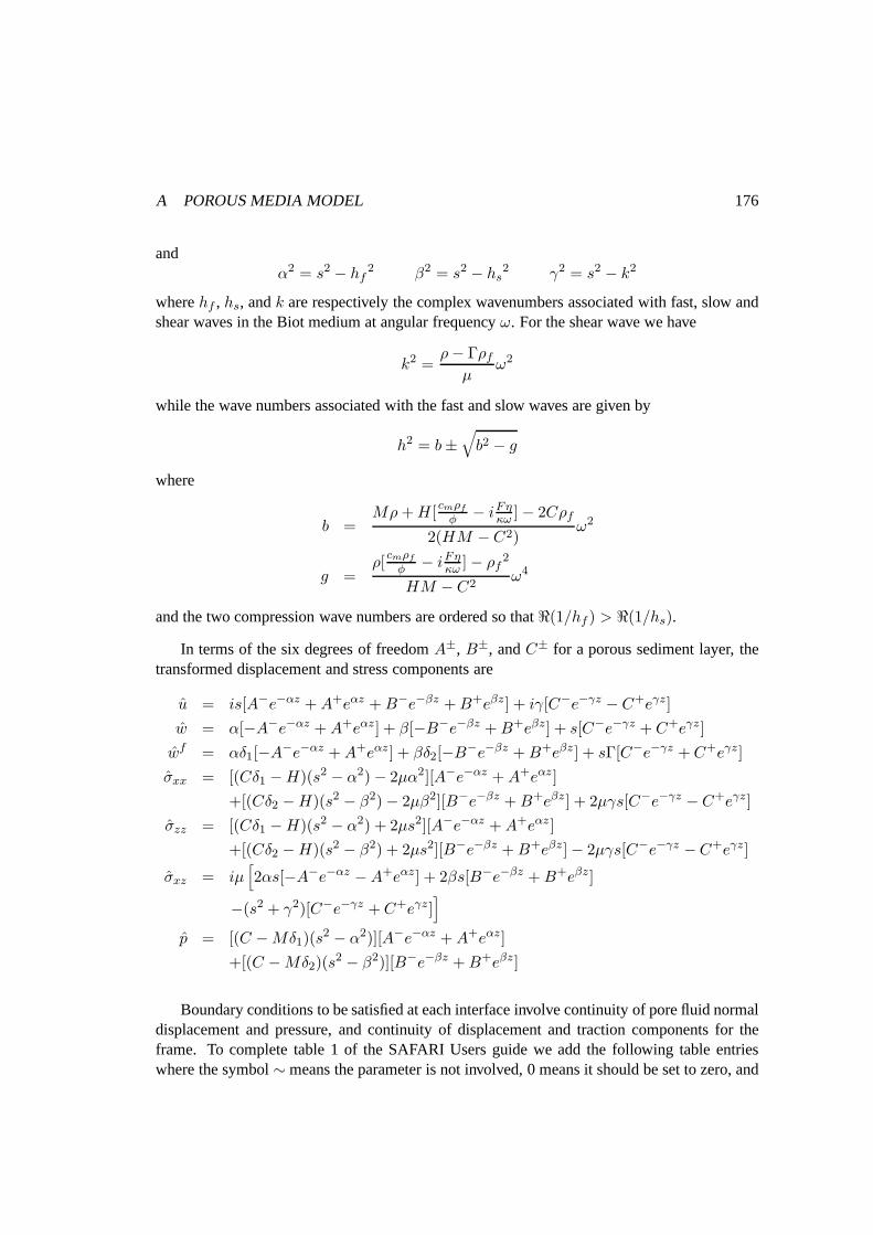
A POROUS MEDIA MODEL 176
andα2 = s2 − hf
2 β2 = s2 − hs2 γ2 = s2 − k2
wherehf , hs, andk are respectively the complex wavenumbers associated with fast, slow andshear waves in the Biot medium at angular frequencyω. For the shear wave we have
k2 =ρ− Γρf
µω2
while the wave numbers associated with the fast and slow waves are given by
h2 = b±√
b2 − g
where
b =Mρ+H[
cmρfφ
− iFηκω
]− 2Cρf
2(HM −C2)ω2
g =ρ[
cmρfφ
− iFηκω
]− ρf2
HM − C2ω4
and the two compression wave numbers are ordered so thatℜ(1/hf ) > ℜ(1/hs).
In terms of the six degrees of freedomA±, B±, andC± for a porous sediment layer, thetransformed displacement and stress components are
u = is[A−e−αz +A+eαz +B−e−βz +B+eβz] + iγ[C−e−γz − C+eγz]
w = α[−A−e−αz +A+eαz] + β[−B−e−βz +B+eβz] + s[C−e−γz + C+eγz ]
wf = αδ1[−A−e−αz +A+eαz ] + βδ2[−B
−e−βz +B+eβz ] + sΓ[C−e−γz +C+eγz]
σxx = [(Cδ1 −H)(s2 − α2)− 2µα2][A−e−αz +A+eαz]
+[(Cδ2 −H)(s2 − β2)− 2µβ2][B−e−βz +B+eβz ] + 2µγs[C−e−γz − C+eγz]
σzz = [(Cδ1 −H)(s2 − α2) + 2µs2][A−e−αz +A+eαz ]
+[(Cδ2 −H)(s2 − β2) + 2µs2][B−e−βz +B+eβz]− 2µγs[C−e−γz −C+eγz]
σxz = iµ[
2αs[−A−e−αz −A+eαz] + 2βs[B−e−βz +B+eβz]
−(s2 + γ2)[C−e−γz +C+eγz]]
p = [(C −Mδ1)(s2 − α2)][A−e−αz +A+eαz]
+[(C −Mδ2)(s2 − β2)][B−e−βz +B+eβz]
Boundary conditions to be satisfied at each interface involve continuity of pore fluid normaldisplacement and pressure, and continuity of displacementand traction components for theframe. To complete table 1 of the SAFARI Users guide we add thefollowing table entrieswhere the symbol∼ means the parameter is not involved, 0 means it should be set to zero, and

A POROUS MEDIA MODEL 177
= means continuity is enforced at the interface. In the following table the first four columnscorrespond to the same entries in the Users Guide table, while the last column corresponds tothe negative of the traction componentσzz in adjacent fluid layers.
Type Field parameterw − wf u σzz σxz wf p
Biot/vacuum ∼ ∼ 0 0 ∼ 0Biot/fluid = ∼ = 0 ∼ =Biot/solid = = = = 0 ∼Biot/Biot = = = = = =