oai arxiv org hep ph 0010288
TRANSCRIPT
arX
iv:h
ep-p
h/00
1028
8 v2
16
Mar
200
1
KUNS-1693
hep-th/0010288
Off-Shell d = 5 Supergravity Coupled to
a Matter-Yang-Mills System
Taichiro Kugo∗ and Keisuke Ohashi
∗∗
Department of Physics, Kyoto University, Kyoto 606-8502, Japan
Abstract
We present an off-shell formulation of a matter-Yang-Mills system coupled to su-
pergravity in five-dimensional space-time. We give an invariant action for a general
system of vector multiplets and hypermultiplets coupled to supergravity as well as
the supersymmetry transformation rules. All the auxiliary fields are retained, so that
the supersymmetry transformation rules remain unchanged even when the action is
changed.
∗ E-mail: [email protected]∗∗ E-mail: [email protected]
1 typeset using PTPTEX.sty <ver.1.0>

§1. Introduction
It is a revolutionary and interesting idea that our four-dimensional world may be a ‘3-
brane’ embedded in a higher-dimensional spacetime. In order to investigate various problems
seriously in such brane world scenarios, however, we need to understand supergravity theory
in five dimensions. 1), 2)
We are interested in five-dimensional space-time since it provides us with the simplest
case in which we have a single extra dimension. Also, in a more realistic situation, it is
believed that M-theory, whose low energy effective theory is described by eleven-dimensional
supergravity, is compactified on Calabi-Yau 3-folds and that it can then be described by
effective five-dimensional supergravity theories. 3), 4)
In the framework of the ‘on-shell formulation’ (that is, the formulation in which there are
no auxiliary fields and hence the supersymmetry algebra closes only on-shell), Gunayden,
Sierra and Townsend 5) (GST) proposed such a five-dimensional supergravity theory which
contains general Yang-Mills/Maxwell vector multiplets. Their work was extended recently
by Ceresole and Dall’Agata 6) to a rather general system containing also tensor (linear)
multiplets and hypermultiplets.
However, in various problems we need an off-shell formulation containing the auxiliary
fields with which the supersymmetry transformation laws are made system-independent and
the algebra closes without using equations of motion. For instance, Mirabelli and Peskin 7)
were able to give a simple algorithm based on an off-shell formulation for finding how to
couple bulk fields to boundary fields in a work in which they considered a five-dimensional
super Yang-Mills theory compactified on S1/Z2. They clarified how supersymmetry breaking
occurring on one boundary is communicated to another. Moreover, if we wish to study
problems by adding D-branes to such a system, then, without an off-shell formulation, we
must find a new supersymmetry transformation rule of the bulk fields each time that we
add new branes, since the supersymmetry transformation law in the on-shell formulation
depends on the Lagrangian of the system.
A 5D supergravity tensor calculus for constructing an off-shell formulation has been given
by Zucker. 8) In a previous paper, 9) which we refer to as I henceforth, we derived a more
complete tensor calculus using dimensional reduction from 6D superconformal tensor calcu-
lus. 10) Tensor calculus gives a set of rules in off-shell supergravity: i) transformation laws of
the various types of supermultiplets; ii) composition laws of multiplets from multiplets; and
iii) invariant action formulas. In this paper, we construct an action for a general system of
vector multiplets and hypermultiplets coupled to supergravity based on the tensor calculus
presented in I. This is, in principle, a straightforward task (containing no trial-and-error
2

steps). Nevertheless it requires considerable computations to simplify the form of the action
and transformation laws; in particular, we must perform a change of variables in order to
make the Rarita-Schwinger term canonical by solving the mixing between the gravitino and
matter fermion fields.
In §2, we present an invariant action for the system of vector multiplets. Although a
certain index must be restricted to be of an Abelian group in order for the tensor calculus
formulas to be applicable, we find that the action can in fact be generalized to non-Abelian
cases by a slight modification. The action for the system of hypermultiplets is next given
in §3, where the mass term is also included. In §4, we combine these two systems and
make a first step to simplifying the form of the total action. In §5, we fix the dilatation
gauge and perform a change of variables to obtain the final form of the action, in which
both the Einstein and Rarita-Schwinger terms take canonical forms. This gauge fixing and
change of variables modify the supersymmetry transformation into a combination of the
original supersymmetry and other transformations, which are carried out in §6. In §7, we
give comments on i) the relation to the independent variables used in GST, ii) compensator
components in the hypermultiplets, iii) the gauging of SU(2)R and U(1)R, and iv) the scalar
potential term in the action. We conclude in §8. Appendix A gives a technical proof for the
existence of a representation matrix. In Appendix B, we explicitly show how the manifold
U(2, n)/U(2)×U(n) is obtained as a target space of the hypermultiplet scalar fields for the
case of two (quaternion) compensators. 14)
In this paper, we do not give the tensor calculus formulas presented in our previous paper
I, but we freely refer to the equations given there. For instance, (I 2·3) denotes Eq. (2·3) in
I. For clarity, however, we list in Table I the field contents of the Weyl multiplets, vector
multiplets and hypermultiplets, which we deal with in this paper. (The dilatation gauge
field bµ and spin connection ωabµ are also listed, although they are dependent fields.) The
notation is the same as in I, with one exception: Here we use χi to denote the auxiliary
fermion component of the Weyl multiplet denoted by χi in I.
§2. Vector multiplet action
Let V I ≡ (M I , W Iµ , Ω
I i, Y I ij) (I = 1, 2, · · · , n) be vector multiplets of a gauge group
G, which we assume to be given generally by a direct product of simple groups Gi and U(1)
groups:
G =∏
i
Gi ×∏
x
U(1)x. (Gi : simple) (2.1)
3

Table I. Field contents of the multiplets.
field type restrictions SU(2) Weyl-weight
Weyl multiplet
eµa boson funfbein 1 −1
ψiµ fermion SU(2)-Majorana 2 −1
2
V ijµ boson SU(2) gauge field V ij
µ = V jiµ = V ∗
µij 3 0
Aµ boson gravi-photon Aµ = ez5e
5µ 1 0
α boson ‘dilaton’ α = ez5 1 1
tij boson tij = tji = t∗ij (= −V ij5 ) 3 1
vab boson real tensor vab = −vba 1 1
χi fermion SU(2)-Majorana 232
C boson real scalar 1 2
bµ boson D gauge field bµ = α−1∂µα 1 0
ωµab boson spin connection 1 0
Vector multiplet
Wµ boson real gauge field 1 0
M boson real scalar, M = −W5 1 1
Ωi fermion SU(2)-Majorana 232
Yij boson Y ij = Y ji = Y ∗ij 3 2
Hypermultiplet
Aαi boson Ai
α = εijAβj ρβα = −(Aα
i )∗ 232
ζα fermion ζα ≡ (ζα)†γ0 = ζαTC 1 2
Fαi boson F i
α = −(Fαi )∗ 2
52
The structure constant fIJK of G, [tI , tJ ] = −fIJ
KtK , is nonvanishing only when I, J and
K all belong to a common simple factor group Gi, and then it is the same as the structure
constant of the simple group Gi. The gauge coupling constants can, of course, be different
for each factor group Gi and U(1)x, but for simplicity, we write the G transformation of
4

M I , for instance, in the form δG(θ)M I = g[θ,M ]I = −gfJKIθJMK . The quantity g here,
therefore, should be understood as representing the coupling constant gi of Gi when I ∈ Gi.
(M here in [θ,M ] denotes a matrix such that M = M ItI .)
In addition to these V I (I = 1, 2, · · · , n), we have a special vector multiplet called the
‘central charge vector multiplet’, which consists of the dilaton α = ez5 and the gravi-photon
Aµ = ez5e
5µ among the Weyl multiplet:
V I=0 = (M I=0, W I=0µ , ΩI=0 i, Y I=0 ij) ≡ (α, Aµ, 0, 0). (2.2)
We henceforth extend the group index I to run from 0 to n and use I = 0 to denote this
central charge vector multiplet as written here. Corresponding to this extension, the gauge
group G should also be understood to include the central charge Z as one of the Abelian
U(1)x factor groups. Note that the fermion and auxiliary field components of this multiplet
are zero: ΩI=0 = Y I=0 = 0. Thus the number of scalar and vector components is each n+1,
while the number of Ω and Y components is each n, at this stage. (Below the number of
scalar components is reduced by 1 through D-gauge fixing.)
In I, we show that we can construct a linear multiplet L = (Lij , ϕi, Ea, N), denoted by
f(V ), from vector multiplets V I using any homogeneous quadratic polynomial in M I ,
f(M) = 12fIJM
IMJ , (2.3)
where I, J run from 0. The vector component Ea of a linear multiplet is subject to a
‘divergenceless’ constraint, and it can be replaced by an unconstrained anti-symmetric tensor
(density) field Eµν when L is completely neutral under G. The explicit expression for the
components of this multiplet, L = f(V ), Lij , ϕi, Ea, N and Eµν , in terms of those of V I
is given in Eqs. (I 5·3) and (I 5·5). We also have the V-L action formula in Eq. (I 5·7),
which gives an invariant action for any pair consisting of an Abelian vector multiplet V =
(M,Wµ, Ωi, Y ij) and a linear multiplet L = (Lij , ϕi, Ea (orEµν), N):
e−1LVL = Y ijLij + 2iΩϕ+ 2iψiaγ
aΩjLij + 12M(N − 2iψbγ
bϕ− 2iψiaγ
abψjbLij)
− 12Wa(E
a − 2iψbγbaϕ + 2iψi
bγabcψj
cLij) . (2.4)
This formula is valid only when the liner multiplet L carries no gauge group charges or is
charged only under the abelian group of this vector multiplet V . When the linear multiplet
carries no charges, the constrained component Ea can be replaced by the unconstrained
anti-symmetric tensor Eµν , and the action formula (2.4) can be rewritten in a simpler form:
e−1LVL = Y ijLij + 2iΩϕ+ 2iψiaγ
aΩjLij + 12M(N − 2iψbγ
bϕ− 2iψiaγ
abψjbLij)
+ 14e
−1Fµν(W )Eµν . (2.5)
5
Now we use this invariant action formula (2.5) to construct a general action for our set of
vector multiplets V I. Since this formula applies only to an Abelian vector multiplet V , we
first choose all the Abelian vector multiplets V A from V I, and, for each abelian index A
we prepare a G-invariant quadratic polynomial fA(M) to construct a neutral linear multiplet
LA = fA(V ) using Eqs. (I 5·3) and (I 5·5). We apply the V-L action formula (2.5) to these
pairs of V A and LA = fA(V ) and sum over all the Abelian indices A. Then we rewrite
super-covariantized quantities like Gab(W ), DaMI , DaΩ
I , etc., as non-supercovariantized
quantities:
GIab(W ) = GI
ab(W ) + 4iψ[aγb]ΩI ,
DaΩIi = DaΩ
Ii + (14γ ·GI(W ) + 1
2/DM I − Y I)ψi
a + iγbcψia(ψbγcΩ
I) − iγbψia(ψbΩ
I),
DaMI = DaM
I − 2iψaΩI . (2.6)
Here, Dµ is the usual covariant derivative, which is covariant only with respect to the ho-
mogeneous transformations Mab, Uij , D and G. Then, interestingly, many cancellations
occur, and the resultant expression is no more complicated than that written with superco-
variantized quantities. Using the notation
fA ≡ fA(M) = 12fA,JKM
JMK , fA,J ≡ ∂fA
∂MJ, fA,JK ≡ ∂2fA
∂MJ∂MK, (2.7)
the result is given by
Y AijLAij + 2iΩAϕA + 2iψiaγ
aΩAjLAij
= fA
(2Y A ·t− 4iψ ·γtΩA − 8iΩAχ
)
+ fA,J
−Y A ·Y J + 2iΩA( /D − 12γ ·v + t)ΩJ + iΩAγa(1
2γ ·G+ /DM)Jψa
− 2(ΩAγaγbcψa)(ψbγcΩJ) + 2(ΩAγaγbψa)(ψbΩ
J)
+ fA,JK
−2iΩA(14γ ·G− 1
2 /DM + Y )JΩK − iΩJY AΩK
+ 2(ΩAγabΩJ)(ψaγbΩK) + 2(ΩAγaΩJ)(ψaΩ
K)
+ 2(ψi ·γΩAj)(ΩJ(iΩ
Kj) )
, (2.8)
12M
A(NA − 2iψbγbϕA − 2iψi
aγabψj
bLAij) + 14e
−1FAµν(W )Eµν
A
= 12fA,JDaMA(DaM
J − 2iψbγaγbΩJ )
+ 12fAM
A
−4C − 16t·t− 12αFab(A)(4vab + iψcγ
abcdψd)
+ 8iψ ·γχ+ 4iψaγabtψb
6

+ 12fA,JM
A
4t·Y J − 16iΩJχ− 8iψ ·γtΩJ + 2ig[Ω, Ω]J
− 12GJab(W )(4vab + iψcγ
abcdψd)
+ 12fA,JKM
A
−14G
J(W )·GK(W ) + 12DaM
JDaMK − Y J ·Y K
+2iΩJ( /D − 12γ ·v + t)ΩK + iψa(γ ·G− 2 /DM)JγaΩK
+(ΩJγabΩK)(ψaψb) − 2(ψiaγ
abψjb)(Ω
Ji Ω
Kj )
−4(ψaγabcΩK)(ψbγcΩ
K) + 4(ψ[aγb]ΩJ )(ψaγbΩK)
−2(ψaΩJ )(ψaΩK)
−14G
Aµν(W )
(fA(4vµν + iψργ
µνρσψσ) + ifA,JKΩJγµνΩK
+ fA,J(GJµν(W ) − 2iψλγµνγλΩJ)
)
− e−1 14fA,JKǫ
λµνρσWAλ F
Jµν(W )FK
ρσ(W ) . (2.9)
Here and throughout this paper, we use the following convention for the SU(2) triplet
quantities X ij, like tij, Y Iij and V ijµ : If their SU(2) indices are suppressed, they represent
the matrix X ij, so that Xψi, when acting on an SU(2) spinor ψi like ΩIi, represents X i
jψj,
and, similarly, Xψi = Xijψj , as obtained by lowering the index i on both sides. X · Y , for
two triplets X and Y , represents tr(XY ) = X ijY
ji = −X ijYji = −X ijYij, and X ·X is also
written X2. For instance, ΩAY JΩK in the above represents ΩAiY JΩKi = ΩAiY J
ijΩKj.
The action is given by the sum of Eqs. (2.8) and (2.9), where the indices J and K
run over the whole group G, while the (external) index A of fA(M) is restricted to run
only over the Abelian subset of G. However, interestingly, this action can be shown to be
totally symmetric with respect to the three indices A, J and K of fA,JK if J and K are
also restricted to the Abelian indices. In view also of the fact that this action formula itself
gives an invariant action, including the case of non-Abelian indices for J and K, we suspect
that this action gives an invariant action even if we extend the the index A of fA(M) to I
running over the whole group G. In that case, the function fI(M) for the indices I belonging
to the non-Abelian factor groups Gi of G should, of course, be a function giving the adjoint
representation of Gi to satisfy the G invariance, and the Chern-Simons term should also be
generalized to the corresponding one. (A similar situation also exists in the 6D case. 10))
Then the product M IfI(M) becomes a general G-invariant homogeneous cubic polynomial
in M , which, with a sign change, is called a ‘norm function’ and denoted N (M), following
Gunayden, Sierra and Townsend: 5)
N (M) ≡ cIJKMIMJMK (= −M IfI(M)). (2.10)
Here the coefficient cIJK is totally symmetric with respect to the indices. Now the resul-
7
tant action is characterized solely by this cubic polynomial N (M), and we find the vector
multiplet action
e−1LVL
= +12N
(4C + 16t·t+ 1
2αFab(A)(4vab + iψcγabcdψd) − 8iψ ·γχ− 4iψaγ
abtψb
)
−NI
2t·Y I − 8iΩIχ− 4iψ ·γtΩI + ig[Ω, Ω]I
−GIab(W )(vab + i
4ψcγabcdψd)
− 12NIJ
−14GI(W )·GJ(W ) + 1
2DaM
IDaMJ − Y I ·Y J
+2iΩI( /D − 12γ ·v + t)ΩJ + iψa(γ ·G(W ) − 2 /DM)IγaΩJ
−2(ΩIγaγbcψa)(ψbγcΩJ ) + 2(ΩIγaγbψa)(ψbΩ
J )
−NIJK
−iΩI(14γ ·G(W ) + Y )JΩK
+ 23(ΩIγabΩJ)(ψaγbΩ
K) + 23(ψi ·γΩIj)(ΩJ
(iΩKj) )
+ e−1LC-S , (2.11)
where NI = ∂N /∂M I , NIJ = ∂2N /∂M I∂MJ , etc., and LC-S is the Chern-Simons term:
LC-S = 18cIJKǫ
λµνρσW Iλ
(F J
µν(W )FKρσ(W ) + 1
2g[Wµ,Wν ]
JFKρσ(W )
+ 110g
2[Wµ,Wν ]J [Wρ,Wσ]K
). (2.12)
We have checked the supersymmetry invariance of this action for general non-Abelian
cases as follows. When the gauge coupling g is set equal to zero, the action reduces to one
with the same form as that for the Abelian case, and thus the invariance is guaranteed by
the above derivation. When g is switched on, the covariant derivative Dµ comes to include
the G-covariantization term −gδG(Wµ), and the field strength Fµν(W ) comes to include the
non-Abelian term −g[Wµ,Wν ]. We, however, can use the variables Dµφ (φ = M I , ΩI) and
Fµν(W ) as they stand in the action and in the supersymmetry transformation laws, keep-
ing these g-dependent terms implicit inside of them. Then, we have only to keep track of
explicitly g-dependent terms and make sure that these terms vanish in the supersymme-
try transformation of the action. The explicitly g-dependent terms in the action are only
the term −igNI [Ω, Ω]I , aside from those in the Chern-Simons term. The Chern-Simons
term is special because it contains the gauge field W Iµ explicitly, and its supersymmetry
transformation as a whole yields no explicit g-dependent terms, as we show below. In the
supersymmetry transformations δφ, explicitly g-dependent terms do not appear for φ = M I ,
ΩI , GIµν(W ) or F I
µν(W ), but appear only in δY Iij , δ(DµMI) and δ(DµΩ
I). (For the latter
8

two, the supersymmetry transformation ofWµ contained implicitly in Dµ produces additional
explicitly g-dependent terms). It is easy to see that all these g-dependent terms cancel out
in the transformation of the action.
In carrying out such computations, it is convenient to use a matrix notation to represent
the norm function N . One can show that, for any G-invariant N (M) = cIJKMIMJMK ,
there is a set of hermitian matrices TI which satisfies
cIJK = 16
tr(TI TJ , TK) (2.13)
and gives a representation of G up to normalization constants ci for each simple factor group
Gi; that is, the rescaled matrices tI ≡ iTI/c[I], where c[I] = ci for I ∈ Gi and c[I] = 1 for
I ∈ U(1)x, satisfy
[tI , tJ ] = −fIJKtK . (2.14)
In Appendix A, we give a simple example of the representation of G which realizes these
properties. Using the matrix notation X ≡ XITI , we have
N ≡ cIJKMIMJMK = 1
3 tr(M3),
NIXI = tr(XM2), NIJX
IY J = tr(XY , M),NIJKX
IY JZK = tr(XY , Z). (2.15)
With these expressions, we can simply use cyclic identities for the trace instead of referring
to various cumbersome identities for cIJK resulting from its G-invariance property. Note the
difference from the ordinary matrix notation X ≡ XItI : In the present case we have the
relations ˜[X, Y ] = [X, Y ]ITI = −fIJKXIY JTK = [X, Y ] = [X, Y ], since fIJ
K is nonvanishing
only when I, J,K belong to a common simple factor group Gi.
Using this matrix notation for the gauge field W Iµ and the field strength F I
µν , we can define
the matrix-valued 1-form as W ≡ Wµdxµ and the 2-form as F ≡ 1
2Fµνdx
µdxν = dW − gW 2
(where gW 2 = gW ,W/2), with which the Chern-Simons term (2.12) can be rewritten in
the form∫
LC-S d5x =
∫16 tr
(W F F + 1
4W , gW 2F + 110W gW 2 gW 2
). (2.16)
For an arbitrary variation of W Iµ , i.e., δW = X in the matrix-valued 1-form notation, we
find δF = dX − g ˜W,X. Using the Bianchi identity DF = dF − g ˜[W,F ] = 0 and the
properties g ˜W,X = gW ,X = gW, X, g ˜[W,F ] = [gW , F ] = [gW, F ] and [gW 2,W ] =
[gW 2, W ] = g ˜[W 2,W ] = 0, we can show
δ tr(W F F
)= tr
(3F F X − F , gW 2X
),
9

δ tr(W , gW 2F
)= tr
(4F , gW 2X − 2gW 2 gW 2X
),
δ tr(W gW 2 gW 2
)= tr
(5gW 2 gW 2X
), (2.17)
so that the variation of the Chern-Simons term indeed gives no explicitly g-dependent term,
as claimed above:
δ∫LC-S d
5x =∫
12
tr(F F δW ) . (2.18)
§3. Hypermultiplet action
Now let Hα = (Aαi , ζ
α, Fαi ) (α = 1, 2, · · · , 2r) be a set of hypermultiplets which belongs
to a representation ρ of the gauge group G. Under the G transformation it transforms as
δG(θ)Hα =∑n
I=1 gθIρ(tI)
αβH
β. The ordinary matrix notation used for the vector multiplet
in the preceding section was, for instance, M = M ItI , and the matrix tI denoted an adjoint
representation ad(tI) of G. The representation ρ here can, of course, be different from
the adjoint representation ad. However, to avoid cumbersome expressions, we simplify the
matrix notation and write, e.g., MAαi = Mα
βAβi to represent ρ(M)α
βAβi = M Iρ(tI)
αβAβ
i .
(Note MAαi = MαβAβi .)
The invariant action for the hypermultiplets is derived in I from the action in 6D and
is given by Eq. (I 4·11).∗ Again we rewrite the supercovariant derivative Dµ in terms of
the usual covariant derivative Dµ, which is covariant only with respect Mab, Uij , D and G.
(Note that covariantization with respect to the central charge Z transformation is also taken
out.) Then we obtain the following action for the kinetic term of the hypermultiplets:
e−1Lkin = DaAαi DaAi
α − 2iζ α /Dζα + i2α ζ
αγ ·F (A)ζα − iζ αγ ·vζα+ 2igζ αMα
βζβ + Aαi (t+ gM)2Ai
α − 4iψiaζαγ
bγaDaAαi
+
2iζαγabRab
i(Q) − 8iζαχi
+ iαψi
aγabcζαFbc(A) − 4iψiaγbζαvab + 4iψajγ
aζαtij
−8igΩiα
βζβ + 4igψiaγ
aMαβζβ
Aα
i
− 2iψ(ia γ
abcψj)c Aα
j DbAαi
+
C + 14R(M) + i
2 ψaγabcRbc(Q)
−2iψaγaχ+ 1
8α2 F (A)2 − v2 + 2t·t
− i4αψaγ
abcdψbFcd(A) + iψaψbvab − iψi
aγabψj
b tij
A2
∗ This action can also be derived if we make a linear multiplet L = dαβHα ×ZHβ from the hypermul-
tiplets Hα and their central-charge transforms ZHβ by using the formula (I 5·6), and then apply the linear
multiplet action formula (I 5·9) to it.
10

+ 2gY ijαβAα
i Aβj + 4igψ(i
a γaΩ
j)αβAα
i Aβj
+ 2igψ(ia γ
abψj)b Aα
i MαβAβj + (1 −AaAa/α
2)F αi F i
α
+ ψaγbψcζαγabcζα − 1
2ψaγbcψaζ
αγbcζα , (3.1)
where the contraction between a pair with a barred index α and α is defined as
Aαi Aαj ≡ Aβ
i dβαAαj, A2 ≡ Aα
i Aiα, ζ αζα ≡ ζβdβ
αζα, (3.2)
by using the G-invariant metric dαβ introduced in Eqs. (I B·22) and (IB·23). This metric
dαβ is, in its standard form, diagonal and takes the values ±1. 11) Note in the above that
(t+ gM)2Aiα = tikt
kjAj
α + 2gMαβtijAβj + gMαγgM
γβAβi with our present convention. The
hypermultiplets can have masses, and the invariant action for the mass term is given by
Eq. (I 4·14), which reads
e−1Lmass = mηαβ
−AaDaAαiAiβ − (1 −AaAa/α
2)αFαiAiβ
−2iψiaζαA
aAβi + αAiα(t+ gM)Aiβ
+i(−αζαζβ + Aaζαγaζβ)
+2iAαi(−αψiaγ
aζβ + ψiaγ
abζβAb)
+iAαiAβj(−αψiaγ
abψjb + ψi
aγabcψj
cAb)
. (3.3)
(Note that m is a dimensionless parameter, and the actual mass is proportional to m〈α〉.)Here ηαβ is a symmetric G-invariant tensor. 11) Interestingly, this mass term turns out to
be automatically included in the previous kinetic term action (3.1), and it need not be
considered separately, provided that we complete the square for the terms containing the
auxiliary fields Fαi in Lkin + Lmass. (Essentially the same observation is made in Ref. 11).)
Doing so, the Fαi terms become
(1 − AaAa/α2)F α
i F iα with Fα
i ≡ Fαi + 1
2mα(d−1)γ
αηγβAβi , (3.4)
and then, all the other terms in Lmass can be absorbed into the kinetic Lagrangian Lkin if
we extend the gauge index I of the generators tI acting on the hypermultiplets to run also
from 0 and introduce
(gtI=0)αβ ≡ 1
2m(d−1)γαηγβ , (3.5)
so that gWµ in Dµ and M are now understood to be
gWµ =n∑
I=1
W Iµ (gtI) + Aµ(gt0) ,
gM =n∑
I=1
M I(gtI) + α(gt0) . (3.6)
11

§4. First step in rewriting the action
Now, the invariant action for our Yang-Mills-matter system coupled to supergravity is
given by the sum L = LVL[(2.11)] + Lkin[(3.1)], where in Lkin the F2 term is replaced by
(3.4), and Eq. (3.6) is understood.
We first note that the auxiliary fields C and χ appear in the action L in the form of
Lagrange multipliers:
C(A2 + 2N ) − 8iχ(ζ +Ω) , (4.1)
where ζi and Ωi are defined as
ζi ≡ Aαi ζα = Aβ
i dβαζα, Ωi ≡ NIΩ
Ii . (4.2)
That is, A2 = −2N and ζi = −Ωi are equations of motion. Although we do not use
equations of motion, we can rewrite the terms multiplied by A2, A2X, as −2NX with
the shift C → C + X, and, similarly, we can rewrite the terms Xζ as −XΩ with the shift
χ→ χ+iX/8. Using this, we replace all the terms containing the factor A2 and all the terms
containing the factor ζi = Aαi ζα in Lkin by those multiplied by N and by Ωi, respectively.
When doing this, we also rewrite the covariant derivative Dµ in the following form,
separating the terms containing gauge fields bµ (= α−1∂µα) and V ijµ :
Dµ = ∇µ − δD(bµ) − δU(V ijµ ) − δM(−2eµ
[abb]). (4.3)
The last term appears because the spin connection ωabµ contains the bµ field as
ω abµ = ω0 ab
µ + i(2ψµγ[aψb] + ψaγµψ
b) − 2e [aµ bb] ,
ω0 abµ ≡ −2eν[a∂[µe
b]ν] + eρ[aeb]σeµ
c∂ρeσc . (4.4)
Then, the covariant derivative ∇µ is now covariant only with respect to local-Lorentz and
group transformations, and the spin connection is that with bµ set equal to 0:
∇µ = ∂µ − δM (ωabµ |bµ=0) − δG(Wµ). (4.5)
We perform this separation of the bµ and V ijµ gauge fields also for R(M) and Ri
ab(Q). This
separation also yields several terms proportional to A2 and ζi, which also can be rewritten
as terms proportional to N and Ωi with shifts of C and χ.
Thus, we finally define C ′ and χ′ in terms of C and χ as follows:
C ′ = C + 14R(M) + i
2ψaγ
abcRbc(Q) − 2iψaγaχ+ 1
8α2 F (A)2
− v2 − i4α ψaγ
abcdψbFcd(A) + iψaψbvab − iψi
aγabψj
b tij
12

+ 94b
2 + 52t·t+ 3
2e−1∇µ(eb
µ) + 12V
ija V
aij + iψi
bγbacψj
cVa ij ,
χ′i = χi − 1
4γabRabi(Q) + 1
8αγabcψaiFbc(A)
+ 12γbψaiv
ab + 12tγ ·ψi + γaγb(1
2Vb − 3
4bb)ψai . (4.6)
We also separate and collect the terms containing Fab(A) and the auxiliary fields vab, V ijµ ,
tij ,Y Iij , F iα. Then the action L is found to take the following form at this stage:
L = L′hyper + L′
vector + LC-S + L′aux ,
e−1L′hyper = ∇aAα
i ∇aAiα − 2iζ α( /∇ + gM)ζα
+ Aαi (gM)2
αβAi
β − 4iψiaγ
bγaζα∇bAαi − 2iψ(i
a γabcψj)
c Aαj ∇bAαi
+ Aαi
(8igΩi
αβζβ − 4igψi
aγaMαβζ
β
+ 4igψ(ia γ
aΩj)αβAβ
j − 2igψ(ia γ
abψj)b MαβAβ
j
)
+ ψaγbψcζαγabcζα − 1
2ψaγbcψaζ
αγbcζα ,
e−1L′vector = N
(−1
2R(M)|b=0 − 2iψµγµνρ∇νψρ + (ψaψb)(ψcγ
abcdψd + ψaψb))
−NI
−4iΩIγµν∇µψν + 2ΩIγabcψaψbψc
+ ig[Ω, Ω]I − i4ψcγ
abcdψdFIab(W )
− 12
(NIJ − NINJ
N) (
−14F
I(W )·F J(W ) + 12∇aM
I∇aMJ)
− 12NIJ
+2iΩI /∇ΩJ + iψa(γ ·F (W )− 2 /∇M)IγaΩJ
−2(ΩIγaγbcψa)(ψbγcΩJ) + 2(ΩIγaγbψa)(ψbΩ
J)
−NIJK
−iΩI 14γ ·F J(W )ΩK
+ 23(ΩIγabΩJ)(ψaγbΩ
K) + 23(ψi ·γΩIj)(ΩJ
(iΩKj) )
,
e−1L′aux = C ′(A2 + 2N ) − 8iχ′(ζ +Ω) − ba∇aN
+ 2N(v − 1
2αF (A) +NI
4N F I(W ))2
− i(v − 1
2αF (A))ab(
2N ψaψb + ζ αγabζα − 4ψaγbΩ − 12NIJΩ
IγabΩJ)
−NV ija V
aij − V a
ij
(2Aαi∇aAj
α + 4iΩiψja − iNIJΩ
IiγaΩJj)
− 12NIJ(Y ijI −M Itij)(Y J
ij −MJtij)
+ (Y Iij −M Itij)(2Ai
α(gtI)αβAj
β + iNIJKΩJiΩKj)
+(1 − A2/α2
)(F α
i − F αsol i)(F i
α − F isol α) , (4.7)
where F αsol i is the solution of the equation of motion for Fα
i ,
F αsol i = −1
2αm(d−1)αγη
γβAβi = −α(gtI=0)αβAβi = (gM0t0)
αβAβ
i . (4.8)
13

Here it is quite remarkable that all the terms explicitly containing either bµ (= α−1∂µα) or
Fµν(A) have completely disappeared from the action, other than L′aux, except for the terms
contained in the form M I and F I(W ). That is, α = M I=0 and Fµν(A) = F I=0µν (W ), which
carry the index I = 0, do not appear by themselves, but are only contained in the action in
a form that is completely symmetric with the components with I ≥ 1.
§5. Final form of the action
In view of the action (4.7), we note that the Einstein term can be made canonical if
N (M) = 1. (5.1)
N (M) is a cubic function of M I , but we fortunately have local dilatation D symmetry, so
that we can take N (M) = 1 as a gauge fixing condition for the D gauge. 12)
However, the action (4.7) is still not in the final form, since there remains a mixing
kinetic term 4iNIΩIγµν∇µψν between the Rarita-Schwinger field ψi
µ and the gaugino field
component Ωi = NIΩIi . If we had superconformal symmetry, we could remove the mixing
simply by imposing
NIΩIi ≡ Ωi = 0 (5.2)
as a conformal S supersymmetry gauge fixing condition. Unfortunately, we already fixed
the S gauge when performing the dimensional reduction from 6D to 5D, and thus we no
longer have such S symmetry. Therefore we here must remove the mixing by making field
redefinitions. The proper Rarita-Schwinger field is found to be
ψNµi = ψµi −
1
3N γµΩi . (5.3)
We also redefine the gaugino fields as
λIi ≡ ΩI
i −M I
3N Ωi = PIJΩ
Ji , (5.4)
where PIJ is the projection operator
PIJ ≡ δI
J − M INJ
3N → PIJM
J = PIJNI = 0 . (5.5)
This new gaugino fields λIi satisfy
NIλIi = 0 , (5.6)
so that they correspond to the gaugino fields ΩIi which we would have had if we could have
imposed the S gauge fixing condition (5.2). Note, however, that the number of independent
14

components of λI is the same as that of the original ΩI , since the I = 0 component of the
latter vanishes: ΩI=0 = 0. Note also that Eq. (5.4) and the relation ΩI=0 = 0 lead to
λ0i = − α
3N Ωi, (5.7)
so that Ωi = N IΩIi is now essentially the I = 0 component of λIi .
We have Aαi ζa ≡ ζi = −Ωi on shell, implying that the hypermultiplet fermions ζα contain
the Ωi degree of freedom. To separate it out, we define new hypermultiplet fermions ξα by
ξα ≡ ζα − Aiα
N Ωi . (5.8)
Then, ξα is indeed orthogonal to Aαi on-shell:
Aαi ξα = ζi −
A2
2N Ωi = (ζi +Ωi) −1
2N Ωi(A2 + 2N ) . (5.9)
In the Lagrangian, the quadratic terms of the form ζ αΓζα yield ‘cross terms’ proportional to
Aαi ξα, which do not vanish but can be eliminated by further shifts of the multiplier auxiliary
fields χ and C. Explicitly, we have
ζ α /∇ζα = (ζ α /∇ζα)′ +
1
N(e−1∇µ(eeµ
a) Ωi + 2∇aΩ
i)γa(ζi +Ωi)
+1
2N 2Ω /∇Ω(A2 + 2N )
,
ζ αΓζα = (ζ αΓζα)′ −
2
N ΩiΓ (ζi +Ωi) −1
2N 2ΩΓΩ(A2 + 2N )
, (5.10)
up to a total derivative term in the action, where the primed terms are the ‘diagonal’ parts:
(ζ α /∇ζα)′ ≡ ξα /∇ξα +1
N Ω /∇Ω +1
N 2(ΩiγaΩj)Aα
i ∇aAαj +2
N (ξαγaΩi)∇aAiα ,
(ζ αγabζα)′ ≡ ξαγabξα +1
N ΩγabΩ . (5.11)
Collecting all the contributions from the bilinear terms in ζα, we find that the cross terms
can be eliminated by replacing C ′ and χ′ by the shifted quantities C ′′ and χ′′ defined as
C ′′ = C ′ +1
2N 2
−2iΩ /∇Ω +
(ψaγbψc(Ωγ
abcΩ) − 12ψaγbcψa(Ωγ
bcΩ))
− iΩγ ·(v − 12αF (A))Ω
+
i
N e−1∇µ(eψaγµγaΩ) ,
χ′′i = χ′
i +1
4N
(e−1∇µ(ee
µa) γaΩi + 2 /∇Ωi
)
+ i(γabcΩi(ψaγbψc) − 1
2γbcΩi(ψ
aγbcψa))
+ γ ·(v − 12αF (A))Ωi
. (5.12)
15

Here, in the last term of C ′′, we have also added a contribution from the term −4iψiaγ
bγaζα∇bAαi
in L′hyper, which yields a term proportional to A2 + 2N after partial integration when ζα is
rewritten by using Eq. (5.8).
We now rewrite the action (4.7) by using the field redefinitions (5.3), (5.4) and (5.8)
everywhere. From this point, the Rarita-Schwinger field always stands for the new variable
ψNµ , and we omit the cumbersome superscript N.
Rewriting (4.7) actually involves a very tedious computation. Note, for instance, that
the spin connection ωabµ |bµ=0 contained in the covariant derivative ∇µ and R(M) is given in
Eq. (4.4) in terms of the original Rarita-Schwinger field ψµ, which should also be rewritten
in terms of the new variable ψNµ in Eq. (5.3). Surprisingly, however, all the terms containing
Ωi ≡ N IΩIi completely cancel out in the action if the auxiliary fields are eliminated by the
equations of motion. This action, which is obtained by eliminating the auxiliary fields, is just
the action in the on-shell formulation, which we term the ‘on-shell action’. Since Ωi ∝ λI=0i ,
as noted above, this fact that the Ωi completely disappear is the fermionic counterpart of
the previously observed fact that the M I=0 = α and F I=0µν (W ) = Fµν(A) terms disappeared
from the action. That is, there appear no terms that carry an explicit I = 0 index, and the
upper indices I, J , etc., are always contracted with the lower indices of NI ,NIJ , etc., in the
on-shell action.
We can demonstrate this noteworthy fact as follows. First, we can confirm that the index
I is ‘conserved’ in all the supersymmetry transformation laws of the physical fields (fields
other than the auxiliary fields); that is, the supersymmetry transformation of a physical field
with the index I contains only the terms carrying the same index, and that of a physical field
without the index I contains only the terms carrying no index. Thus the fields Ωi, α and
Fµν(A), carrying the I = 0 index explicitly, appear only in the transformation of those I = 0
fields. This can be confirmed relatively easily, as we see in the next section. Therefore, if such
terms carrying the I = 0 index explicitly remain in the on-shell action, the supersymmetry
invariance of the action implies that the parts of the action containing different numbers of
I = 0 fields are separately supersymmetry invariant. But we know already that the bosonic
I = 0 fields α and Fµν(A) do not appear. Clearly, no such invariant term can be made from
the Ωi without using their superpartners α and Fµν(A). This proves the total cancellation
of the Ωi terms in the on-shell action. (We have also confirmed this cancellation explicitly
by direct rewriting of the action, except for some four-fermion term parts.)
Completing the square of the auxiliary field terms in the action (4.7), we can rewrite the
action in a sum of the on-shell action and the perfect square terms of the auxiliary fields.
The auxiliary fields implicitly contain Ωi-dependent terms in them. This can be seen by
substituting the field redefinitions (5.3), (5.4) and (5.8) into their solutions of the equations
16

of motion. If we redefine the auxiliary fields as follows by subtracting these implicitly Ωi-
dependent terms, then the Ωi-dependent terms completely disappear also from the perfect
square terms of the auxiliary fields, and we have
V ija = V ij
a +1
2N(4iΩ(iψj)
a +2i
3N ΩiγaΩj),
vab = vab −1
2αFab(A) + iψaψb + i
2
3N ψ[aγb]Ω +i
9N 2ΩγabΩ,
Y Iij = PIJY
Jij − 2i
3N λI(iΩj) ,
tij = tij − NIYIij
3N +i
9N 2Ω(iΩj), (5.13)
where PIJ is the projection operator introduced in Eq. (5.5), and we have taken into account
the fact that Y I − M It = PIJY
J − M I(t − NJYJ/3N ). Note that the vector multiplet
auxiliary fields Y I as well as PIJY
J are orthogonal to NI , as are the fermionic partners λI .
The solutions of the equations of motion for these auxiliary fields are now free from the Ωi
and given by
V ijsol a = − 1
2N(2Aα(i∇aAj)
α − iNIJ λIiγaλ
Jj),
vsol ab = − 1
4N
NIFab(W )I − i
(6N ψaψb + ξαγabξα − 1
2NIJ λIγabλ
J),
Y Iijsol = −1
2aIJPK
J Y ijK = −1
2PIJa
JKY ijK = −
(12a
IJ − 13M
IMJ)Y ij
J
with Y ijI ≡ 2A(i
α(gtI)αβAj)
β + iNIJKλJiλKj,
tijsol = − 1
6NM IY ijI = − 1
6N(2A(i
α(gM)αβAj)β + iNIJ λ
IiλJj), (5.14)
where aIJ is the inverse of the metric aIJ of the vector multiplet kinetic terms:
aIJ ≡ −12
∂2
∂M I∂MJlnN = − 1
2N(NIJ − NINJ
N), aIJ ≡ (a−1)IJ . (5.15)
It possesses the properties
aIJMJ = NI/2N → aIJNJ/2N = M I , aIJPK
J = PIJa
JK . (5.16)
We here have assumed that aIJ is invertible. However, there are some interesting cases in
which det(aIJ) = 0. Such a situation implies that some vector multiplets have no kinetic
terms, since aIJ gives the metric of the vector multiplets. We comment on such a possibility
below.
After all of the above calculations, the action is finally found to take the form
L = Lhyper + Lvector + LC-S + Laux ,
17
e−1Lhyper = ∇aAαi ∇aAi
α − 2iξα( /∇ + gM)ξα
+ Aαi (gM)2
αβAi
β − 4iψiaγ
bγaξα∇bAαi − 2iψ(i
a γabcψj)
c Aαj ∇bAαi
+ Aαi
(8igλi
αβξβ − 4igψi
aγaMαβξ
β
+ 4igψ(ia γ
aλj)αβAβ
j − 2igψ(ia γ
abψj)b MαβAβ
j
)
+ ψaγbψcξαγabcξα − 1
2 ψaγbcψaξ
αγbcξα ,
e−1Lvector = −12R(ω) − 2iψµγ
µνρ∇νψρ + (ψaψb)(ψcγabcdψd + ψaψb)
−NI
(ig[λ, λ]I − i
4ψcγ
abcdψdFab(W )I)
+ aIJ
−14F (W )I ·F (W )J + 1
2∇aM
I∇aMJ
+2iλI /∇λJ + iψa(γ ·F (W )− 2 /∇M)IγaλJ
−2(λIγaγbcψa)(ψbγcλJ) + 2(λIγaγbψa)(ψbλ
J)
−NIJK
−iλI 14γ ·F (W )JλK
+ 23(λIγabλJ)(ψaγbλ
K) + 23(ψi ·γλIj)(λJ
(iλKj))
+18
(2ψaψb + ξαγabξα + aIJ λ
IγabλJ)2
+ i14NIF (W )I
(2ψaψb + ξαγabξα + aIJ λ
IγabλJ)
+(Aαi∇aAj
α + iaIJ λIiγaλ
Jj)2
− 14(aIJ −M IMJ)Y ij
I YJ ij . (5.17)
Here Laux represents the perfect square terms of the auxiliary fields, which vanish on shell:
e−1Laux = C ′′′(A2 + 2) − 8iχ′′iAαi ξα
+ 2(v − vsol)2 − (V − Vsol)
ij(V − Vsol)ij
− 3(t− tsol)ij(t− tsol)ij + aIJ(Y I − Y I
sol)ij(Y J − Y J
sol)ij
+(1 − A2/α2
)(F α
i − F αsol i)(F i
α − F isol α) . (5.18)
Here the multiplier term C ′′(A2 + 2N ) − 8iχ′′(ζ + Ω) has been rewritten into the form of
the first line by using Eq. (5.9) and defining C ′′′ in terms of the C ′′ field as
C ′′′ = C ′′ − i4
N χ′′Ω . (5.19)
Expressed in this way, the explicit Ωi have been completely removed from the action. Note
that the final action (5.17) with (5.18) is everywhere written in terms of the new variables,
although the superscript N has been omitted. In particular, the spin connection ωabµ in the
18

covariant derivative ∇µ and R(ω) is the new one given by Eq. (4.4) with the new ψµ used
and bµ set equal to 0. By using this ωabµ , R(ω) is given as usual:
Rµνab(ω) = 2∂[µων]
ab − 2ω[µ[acων]c
b], Rab(ω) ≡ Raccb(ω) , R(ω) ≡ Ra
a(ω) . (5.20)
§6. Supersymmetry transformation
Now we should modify the supersymmetry (Q) transformation δQ(ε), since we have fixed
the D gauge by (5.1) and made various field redefinitions, (5.3), (5.4) and (5.8). The proper
Q transformation is found to be given by the following linear combination of the original
transformations of Q, dilatation D, local-Lorentz M and SU(2) U :
δNQ(ε) = δQ(ε) + δD(ρ(ε)) + δM(λab(ε)) + δU(θij(ε)),
ρ(ε) ≡ − 2i3N εΩ, λab(ε) ≡ 2i
3N εγabΩ, θij(ε) ≡ − 2iN ε(iΩj). (6.1)
The dilatation part δD(ρ(ε)) is determined so as to maintain the D gauge fixing condition
(5.1): (δQ(ε) + δD(ρ(ε)))N = 0. The local-Lorentz part δM (λab(ε)) is fixed by requiring
that the transformation of the funfbein take the canonical form δN(ε)eµa = −2iεγaψN
µ in
terms of the new Rarita-Schwinger field ψNµ . In the first part of this section, we revive the
superscript N to distinguish the new variables from the original ones. Finally, the SU(2)
part δU (θij) is added so that the hypermultiplet scalar field Aiα is transformed in the new
fermion component ξα to yield the form δN(ε)Aiα = 2iεiξα.
To write the supersymmetry transformation rules concisely and covariantly, we should
use the supercovariant derivative Dµ and the supercovariantized curvatures Rµν . But these
supercovariant quantities are also modified by the D gauge fixing and field redefinitions. We
define a new supercovariant derivative DNµ in the usual form, but by using the new gauge
fields and the new supersymmetry transformation:
DNµ = ∂µ − δM(ωNab
µ ) − δU(V ijµ ) − δG(Wµ) − δN
Q(ψNµ ). (6.2)
The relation with the original supercovariant derivative Dµ, which also contains the D
covariantization, is found to be given by
Dµ = DNµ −δD(bNµ )+δM
(2eµ
[abNb] + i9N 2 Ωγµ
abΩ)−δU ( i
3N 2 Ω(iγµΩ
j))−δNQ( 1
3N γµΩ), (6.3)
where bNµ is the supercovariantized bµ (= α−1∂µα) defined as bNµ ≡ α−1DNµα = bµ + 2i
3αN ψNµΩ.
The new curvatures RNab
A are defined as usual by Eq. (I 2·28) by using the new covariant
derivative DNa with flat index a: [DN
a , DNb ] = −RN
abAXA. Hence, using the relation (6.3)
19

between Dµ and DNµ , we can find the relations between the new curvatures and the original
curvatures RabA. The Yang-Mills group G is also regarded as a subgroup of our supergroup,
and so, for example, in the case A = I of G, we find
F Iab(W ) = FNI
ab (W ) + 4i3N Ωγabλ
I + 2i9N 2M
IΩγabΩ . (6.4)
From this point, we again suppress the cumbersome superscript N of ψNµ , ωNab
µ , DNµ , RN
µνA
(FNIµν ) and δN
Q(ε), since every quantity that appears in the following is always one of these
new ones.
As mentioned in the preceding section, we find that the (new) supersymmetry trans-
formation ‘conserves’ the index I, and thus the Ωi ∝ λI=0i , as well as Fab(A) = F I=0
ab (W )
and α = M I=0 (or bµ = α−1∂µα), carrying an I = 0 index, do not explicitly appear in the
transformation laws, unless the transformed field itself carries I = 0. (The only exception is
the transformation δF iα, which contains Aµ = W I=0
µ and α = M I=0 explicitly. However, F iα
is defined to be δZ(α)Aiα with α = M I=0, and so it may be regarded as carrying the index
I = 0 implicitly.) It is quite easy to demonstrate the disappearance of Fab(A) = F I=0ab (W )
and α = M I=0 by direct computation.
To see the disappearance of explicit Ωi factors, however, we have proceeded in the fol-
lowing way. For the physical fields, eµa, ψi
µ,WIµ ,M
I , λI ,Aiα, ξα, we have explicitly computed
their supersymmetry transformation laws and directly checked that the explicit Ωi cancel
out completely. For the auxiliary fields φ = V ijµ , t
ij , vab, Yij ,F i
α, other than χ′′ and C ′′′, such
rigorous computations become quite tedious, and so we checked the cancellation indirectly:
For such auxiliary fields φ, the supersymmetry transformation of φ−φsol, δ(φ−φsol), should
vanish on-shell, that is, when the equations of motion for auxiliary fields are used. (But note
that the equations of motion for the physical fields need not be used.) Therefore, if an Ωi
appears explicitly in δ(φ− φsol), it must be multiplied by the factors (φ− φsol) which vanish
on-shell, or it must appear in the form Ωi + ζi. For the former possibility, we can easily
see whether such terms appear or not, by keeping track of auxiliary fields explicitly. It is
seen that the latter possibility does not occur by confirming that ζi = Aαi ζα never appears
in δ(φ− φsol). Once Ωi is seen to be absent in δ(φ− φsol), it is seen that it does not appear
in δφ either, since φsol consists of physical fields alone, and hence δφsol does not contain any
Ωi explicitly.
Computations to derive transformation laws of the new auxiliary fields χ′′ and C ′′′ directly
from those of the original fields χ and C become terribly tedious, because the relations
between these new and original fields are very complicated. Instead of doing this, we can
use the invariance of the action to find δχ′′ and δC ′′′. Then, since they appear in the form
δC ′′′ (A2+2N )−8iδχ′′i Aαi ξα in δL, we have only to compute the terms whose supersymmetry
20

transformations can yield the factor A2 or Aαi ξα. There are not a great number of such terms
in the action. The cancellation condition for the terms proportional to (A2 +2N ) and Aαi ξα
determines the supersymmetry transformation laws δC ′′′ and δχ′′ as follows:
δχ′′i = 12ε
iC ′′′ + χ′′i(2iεγ ·ψ) − ψja(2iεjγ
aχ′′i) − 12 /∇(Γ εi)
+ i2γ
aΓ εi(ψaγ ·ψ) − i4γ
abcΓ εi(ψaγbψc) + i8γ
abΓ εi(ψcγabψc + 2ψaψb)
−14γ ·vΓ εi − 1
2e−1∇λ(eV
λ)εi + i2e−1∇λ(eψ
iµγ
µλνψjν)εj ,
δC ′′′ = −2ie−1∇µ(eεγµχ′′) − ie−1∇µ(eψaγµγaΓ ε)
+ C ′′′2iεγ ·ψ + 4iχ′′Γ ε . (6.5)
Here Γ is a field-dependent matrix acting on a spinor with an SU(2) index which is defined
by
Γ εi ≡ (−γ ·V + 3t)ijε
j + γ ·vεi + NI
4N γ ·F I(W )εi + NIJ
N λiI(2iλJε) . (6.6)
Note that there appear derivative terms of the transformation parameter, ∂µεi, in these,
implying that χ′′ and C ′′′ are not covariant quantities. For this reason we redefine these
fields once again as follows by adding proper supercovariantization terms:
χi ≡ χ′′i + 12γaΓψi
a , C ≡ C ′′′ + 2iψ ·γχ− iψaγabΓψb . (6.7)
Here we have used the identity (∇µε)Γψa = ψaΓ∇µε in deriving the covariantization terms
for C ′′′.
We must next derive the supersymmetry transformation law for these covariant variables
χ and C from Eq. (6.5). Note here the simple fact that the transformation of any covariant
quantity gives a covariant quantity and hence cannot contain gauge fields explicitly; that
is, gauge fields can appear only implicitly in the covariant derivatives or in the form of
supercovariant curvatures (field strengths). Otherwise, the two sides of the commutation
relation of the transformations would lead to a contradiction. This observation greatly
simplifies the computations of δχ and δC, in which we can discard such explicit gauge field
terms, since they are guaranteed to cancel out anyway.
We now write the final supersymmetry transformation laws derived this way. The Q
transformation laws of the Weyl multiplet are
δeµa = −2iεγaψµ ,
δψiµ = Dµε
i + γµtijε
j + 12γµabε
ivab + NI
12N γµγ ·F I(W )εi + NIJ
3N γµλIi(2iλJε) ,
δV ijµ = −4iε(iγµχ
j) − iε(iγµabRabj)(Q) + 4iε(iγ ·(v + NI
4N F I(W ))ψj)
µ
− 6i(εψµ)tij + 4NIJ
N((ψµλ
I)ε(iλj)J − (ελI)ψ(iµλ
j)J),
21
δtij = 4iε(iχj) + iε(iγ ·Rj)(Q) + 2iNIJ
3N(ε(i /DM Iλj)J − (ελI)Y Jij
),
δvab = −2iεγabχ− i2 εγabγ ·R(Q) + i
4 εγabcdRcd(Q) − iεRab(Q) ,
δχi = 12εiC − 1
2( /DΓ ′)εi − 1
4γ ·vΓ ′εi + 1
4γ ·R(U)εi
+12γ
aΓ ′(γatε
i + 12γabcε
ivbc + NI
12N γaγ ·F I(W )εi − NIJ
3N γaλIi(2iελJ)
),
δC = −2iε /Dχ+ 12 iεγ
ab, Γ ′Rab(Q) + 2i3 εΓ
′χ+ i3 εγ ·vχ ,
δωµab = −2iεγ[aRµ
b](Q) − iεγµRab(Q)
− 2iεγabcdψµ
(vcd + NI
6N F Iab(W )
)+ 2iεψµ
NI
3N F Iab(W )
− 4iεiγabψjµtij + 4NIJ
3N((ελI)ψµγ
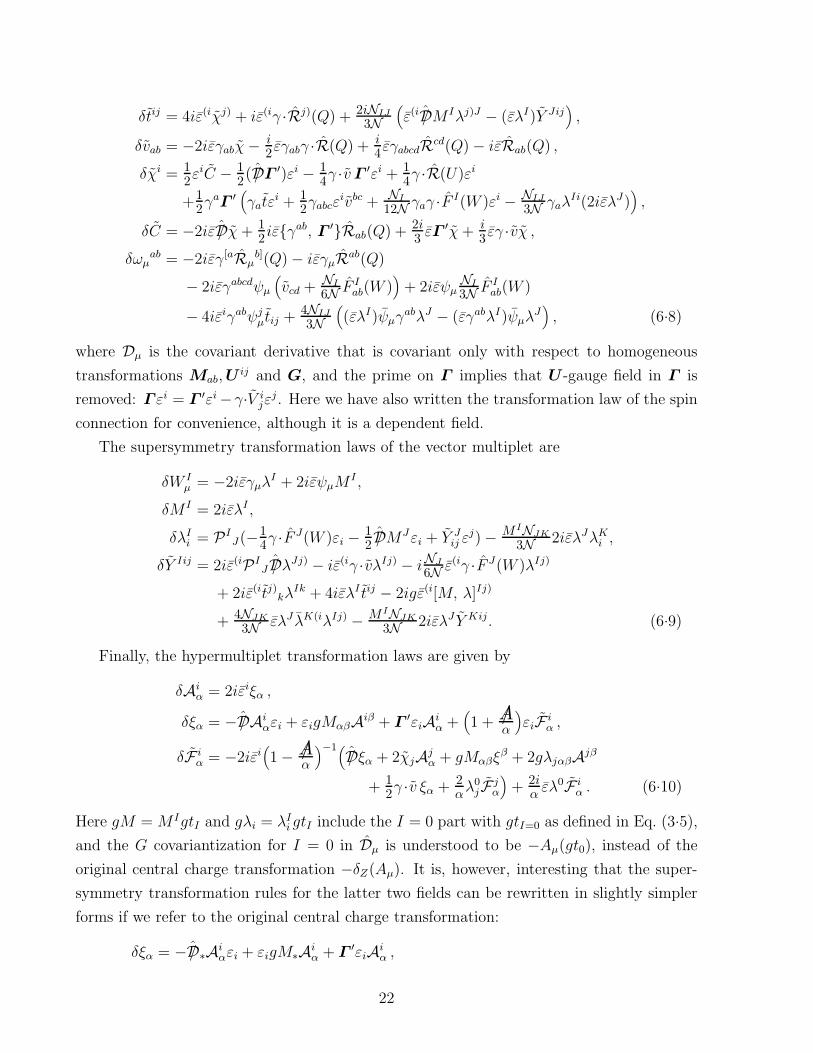
abλJ − (εγabλI)ψµλJ), (6.8)
where Dµ is the covariant derivative that is covariant only with respect to homogeneous
transformations Mab,Uij and G, and the prime on Γ implies that U -gauge field in Γ is
removed: Γ εi = Γ ′εi −γ·V ijε
j . Here we have also written the transformation law of the spin
connection for convenience, although it is a dependent field.
The supersymmetry transformation laws of the vector multiplet are
δW Iµ = −2iεγµλ
I + 2iεψµMI ,
δM I = 2iελI ,
δλIi = PI
J(−14γ ·F
J(W )εi − 12 /DMJεi + Y J
ij εj) − M INJK
3N 2iελJλKi ,
δY Iij = 2iε(iPIJ /DλJj) − iε(iγ ·vλIj) − iNJ
6N ε(iγ ·F J(W )λIj)
+ 2iε(itj)kλIk + 4iελI tij − 2igε(i[M, λ]Ij)
+ 4NJK
3N ελJ λK(iλIj) − M INJK
3N 2iελJ Y Kij. (6.9)
Finally, the hypermultiplet transformation laws are given by
δAiα = 2iεiξα ,
δξα = − /DAiαεi + εigMαβAiβ + Γ ′εiAi
α +(1 + /A
α
)εiF i
α ,
δF iα = −2iεi
(1 − /A
α
)−1(/Dξα + 2χjAj
α + gMαβξβ + 2gλjαβAjβ
+ 12γ ·v ξα + 2
αλ0jF j
α
)+ 2i
α ελ0F i
α . (6.10)
Here gM = M IgtI and gλi = λIi gtI include the I = 0 part with gtI=0 as defined in Eq. (3.5),
and the G covariantization for I = 0 in Dµ is understood to be −Aµ(gt0), instead of the
original central charge transformation −δZ(Aµ). It is, however, interesting that the super-
symmetry transformation rules for the latter two fields can be rewritten in slightly simpler
forms if we refer to the original central charge transformation:
δξα = − /D∗Aiαεi + εigM∗Ai
α + Γ ′εiAiα ,
22

δF iα = −2iεi
(/D∗ξα + 2χjAj
α + gM ′αβξ
β + 2gλ′jαβAjβ + 12 vξα
)+ 4i
α ε(iλ0j)Fαj .
(6.11)
Here D∗ and M∗ denote that the group action for the I = 0 part is the original central charge
transformation Z; that is,
D∗µ = D′µ − δZ(Aµ), gM∗φ
α = gM ′αβ φ
β + δZ(α)φα, (6.12)
and the primes on D′, gM ′ and gλ′i denote that the I = 0 parts are omitted.∗ The central
charge transformation given in Eq. (I 4·5) can be rewritten in terms of our new variables,
and reads, explicitly for Aiα and ξα, as δZ(α)Ai
α = F iα and
δZ(α)ξα = −(
/D∗ξα + 2χjAjα + gM ′
αβξβ + 2gλ′jαβAjβ + 1
2 vξα)− 2
αλ0jF j
α . (6.13)
The last equation is equivalent to the central charge property of the Z transformation on
Aiα, 0 = α [δZ , δQ(ε)]Ai
α = 2iεiδZ(α)ξα − αδQ(ε)(F iα/α), which can also be rewritten in the
following form, with gλj∗ ≡ gλ′j + (λ0j/α)δZ(α):
/D∗ξα + 2χjAjα + gM∗ξα + 2gλj∗Aj
α + 12v ξα = 0 . (6.14)
For convenience, we list here the explicit forms of the covariant derivatives appearing in
these transformation laws:
Dµεi =
(∂µ − 1
4γabω
abµ
)εi − Vµ
ijε
j,
Dµtij = Dµt
ij − 4iψ(iµ χ
j) − iψ(iµ γ ·Rj)(Q) − 2iNIJ
3N(ψ(i
µ /DM Iλj)J − ψµλI Y Jij
),
Dµvab = Dµvab + 2iψµγabχ+ i2ψµγabγ ·R(Q) − i
4ψµγabcdRcd(Q) + iψµRab(Q) ,
Dµtij = ∂µt
ij − 2V (iµ k t
j)k, Dµvab = ∂µvab + 2ωµ[acvb]c ,
DµMI = DµM
I − 2iψµλI , DµM
I = ∂µMI − g[Wµ, M ]I ,
DµFab(W )I = DµFab(W )I − 4iψµγ[aDb]λI − 2iψµRab(Q)M I − 4iψµγ ·vγabλ
I
− 8iψµλI vab − 4iψµγabtλ
I − NI
3N iψµγ ·F (W )IγabλI + 8NIJ
3N (ψµλJ)λIγabλ
K ,
DµFab(W )I = ∂µFab(W )I − g[Wµ, Fab(W )]I + 2ωµ[acFb]c(W )I ,
DµλIi = Dµλ
Ii + PI
J(14γ ·F (W )Jψµi + 1
2/DMJψµi − Y J
ijψjµ) + M INJK
3N (2iψµλJ)λK
i ,
DµλIi =
(∂µ − 1
4γabωabµ
)λI
i − VµijλIj − g[Wµ, λi]
I ,
DµAiα = DµAi
α − 2iψiµξα , DµAi
α = ∂µAiα − V i
µjAjα − gWµαβAβi,
Dµξα = Dµξα + /DAiαψµi − ψµigMAi
α − Γ ′ψµiAiα −
(1 + /A
α
)ψµiF i
α ,
Dµξα =(∂µ − 1
4γabωabµ
)ξα − gWµαβξ
β. (6.15)
∗ It may be worth mentioning that the transformation rules in Eq. (6.10) can also be rewritten equiva-
lently by making the replacements F iα, D, gM, gλi → F i
α, D′, gM ′, gλ′
i.
23

The supercovariant curvatures Rµν are obtained from [Da, Db] = −RabAXA as noted
above, or can be read directly from the above transformation laws of the gauge field, (6.8),
via the formulas (I 2·29), RµνA = 2∂[µh
Aν]−hC
µ hBν f
′BC
A, and (I 2·24), δhAµ = ∂µε
A+εChBµ fBC
A.
Explicitly, they are given by
Rµνi(Q) = 2D[µψ
iν] + 2γ[µt
ijψ
jν] + γ[µabψ
iν]v
ab
+ NI
6N γ[µγ ·F I(W )ψiν] +
4iNIJ
3N γ[µλIi(λJψν]) ,
Rµνij(U) = 2∂[µV
ijν] − [Vµ, Vν ]
ij + 8iψ(i[µγν]χ
j) + 2iψ(i[µγν]abRabj)(Q)
−4iψ(iµ γ ·
(v + NI
4N F I(W ))ψj)
ν + 6iψµψν tij + 8NIJ
N (ψ[µλI)ψ
(iν]λ
j)J ,
F Iµν(W ) = F I
µν(W ) + 4iψ[µγν]λI − 2iψµψνM
I . (6.16)
§7. Compensators, gauged supergravity and scalar potential
7.1. Independent variables
We have labeled the vector multiplet (M I ,W Iµ , λ
Ii, Y Iij) by the index I, taking 1+n values
from 0 to n. However, it is only the vector component W Iµ that actually has 1+n independent
components. All the others have only n components, since the scalar components M I satisfy
the D gauge condition N (M) = 1, and the fermion and auxiliary fields satisfy the constraints
NIλI = NI Y
I = 0. Thus our parametrizations for them are redundant, although the gauge
symmetry is realized linearly for these variables, and hence is more manifest there.
It is, of course, possible to parametrize these fields with independent variables, as was
done by GST from the beginning in their on-shell formulation. 5) GST parametrized the
manifold M of the scalar fields by φx with curved index x = 1, · · · , n, and the fermions by
λa with tangent index a = 1, · · · , n. We can assign the same tangent index to our auxiliary
fields and write Y a.
The basic correspondence between the GST parametrization and ours is as follows:
GST parametrization our parametrization
N = CIJKhI(φ)hJ(φ)hK(φ) ↔ N = cIJKM
IMJMK
hI(φ) = −√
23M
I |N=1
hI(φ) = − 1√6NI |N=1
(7.1)
From this, various geometrical quantities defined by GST can be translated into their coun-
terparts in our formulation. The metric aIJ of the ambient 1 + n dimensional space is the
24
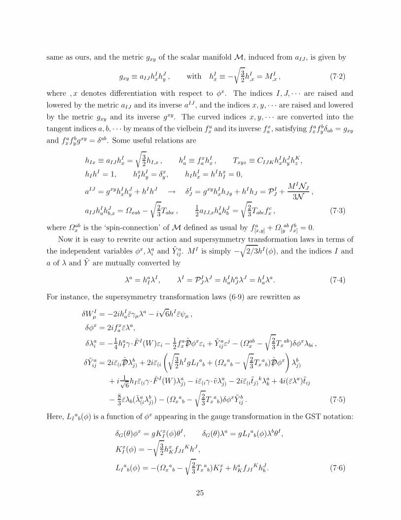
same as ours, and the metric gxy of the scalar manifold M, induced from aIJ , is given by
gxy ≡ aIJhIxh
Jy , with hI
x ≡ −√
32hI
,x = M I,x , (7.2)
where , x denotes differentiation with respect to φx. The indices I, J, · · · are raised and
lowered by the metric aIJ and its inverse aIJ , and the indices x, y, · · · are raised and lowered
by the metric gxy and its inverse gxy. The curved indices x, y, · · · are converted into the
tangent indices a, b, · · · by means of the vielbein fax and its inverse fx
a , satisfying faxf
byδab = gxy
and faxf
byg
xy = δab. Some useful relations are
hIx ≡ aIJhIx =
√32hI,x , hI
a ≡ fxa h
Ix , Txyz ≡ CIJKh
Ixh
Jyh
Kz ,
hIhI = 1, hx
IhIy = δx
y , hIhIx = hIhx
I = 0,
aIJ = gxyhIxh
Jy + hIhJ → δI
J = gxyhIxhJy + hIhJ = PI
J +M INJ
3N ,
aIJhIah
Jb,x = Ωxab −
√23Tabx ,
12aIJ,xh
Iah
Jb =
√23Tabcf
cx , (7.3)
where Ωabx is the ‘spin-connection’ of M defined as usual by fa
[x,y] +Ω ab[y f b
x] = 0.
Now it is easy to rewrite our action and supersymmetry transformation laws in terms of
the independent variables φx, λai and Y a
ij . MI is simply −
√2/3hI(φ), and the indices I and
a of λ and Y are mutually converted by
λa = haIλ
I , λI = PIJλ
J = hIah
aJλ
J = hIaλ
a. (7.4)
For instance, the supersymmetry transformation laws (6.9) are rewritten as
δW Iµ = −2ihI
aεγµλa − i
√6hI εψµ ,
δφx = 2ifxa ελ
a,
δλai = −1
4haIγ ·F I(W )εi − 1
2fax /Dφxεi + Y a
ijεj − (Ωab
x −√
23Tx
ab)δφxλbi ,
δY aij = 2iε(i /Dλb
j) + 2iε(i
(√32h
IgLIab + (Ωx
ab −
√23Tx
ab) /Dφx
)λb
j)
+ i 1√6hI ε(iγ ·F I(W )λa
j) − iε(iγ ·vλaj) − 2iε(itj)
kλak + 4i(ελa)tij
− 83 ελb(λ
a(iλ
bj)) − (Ωx
ab −
√23Tx
ab)δφ
xY bij . (7.5)
Here, LIab(φ) is a function of φx appearing in the gauge transformation in the GST notation:
δG(θ)φx = gKxI (φ)θI , δG(θ)λa = gLI
ab(φ)λbθI ,
KxI (φ) = −
√32h
xKfJI
KhJ ,
LIab(φ) = −(Ωx
ab −
√23Tx
ab)K
xI + ha
KfJIKhJ
b . (7.6)
25

One can see that these transformation laws for the physical components W Iµ , φ
x and λai
agree with the GST result 5) if the auxiliary fields are replaced by their solutions [and 2λa,
2ψµ, 2ε and iγµ(−iγµ) here are identified with λa, ψµ, ε and γµ(γµ) of GST.] One can also
easily rewrite the action and see the agreement with GST for the on-shell part in the absence
of the hypermultiplet.
In the case of the hypermultiplet, Aiα and ξα are independent variables off-shell. However,
on-shell they become mutually dependent variables, since they satisfy the equations of motion
A2 = −2 and Aαi ξα = 0. Moreover, there remains the SU(2) U gauge symmetry, with which
three components of Aiα can be eliminated. (Thus at least four of the Ai
α and two of the ξα can
be eliminated. Generally, compensator components of the hypermultiplets can be eliminated
by equations of motion and the gauge symmetries, as explained below.) It is possible to
separate the variables even off-shell into genuine independent variables and other variables
that vanish on-shell or can be eliminated by gauge fixing. Such independent variables are
those used in the on-shell formulation, for instance, by Ceresole and Dall’Agata, 6) and they
are formally very similar to the GST variables for vector multiplets. Hence, the rewriting of
the hypermultiplet variables can be done in a manner similar to that in the vector multiplet
case. The only complications in this case are the above mentioned separation of the on-shell
(or gauge) vanishing variables, which depend on the number of the compensators (i.e., the
structure of the hypermultiplet manifold).
7.2. Compensator
The D gauge fixing N = 1 was necessary to obtain the canonical form of the Einstein-
Hilbert term. Owing to the equation of motion A2 + 2N = 0, this in turn implies that the
relation
A2 ≡ Aαi dα
βAiβ = −2 (7.7)
must hold on-shell. But this is possible only if some components of the hypermultiplet Aαi
have negative metric. 13) To see this, we recall the fact that the metric dαβ of the hypermul-
tiplet can be brought into the standard form 11)
dαβ =
(12p
−12q
). (p, q : integer) (7.8)
We distinguish the first 2p components of the hypermultiplet Aαi with index α = 1, 2, · · · , 2p
from the rest of the 2q components, and use the indices a and α to denote the former 2p and
the latter 2q components, respectively. Also taking account of the hermiticity Aiα = −(Aα
i )∗,
the quadratic terms of the hypermultiplet read
A2 ≡ Aαi dα
βAiβ = −(Aa
i )∗(Aa
i ) + (Aαi )∗(Aα
i ) ≡ −|Aai |2 + |Aα
i |2,
26

∇µAαi ∇µAi
α = −(∇µAai )
∗(∇µAai ) + (∇µAα
i )∗(∇µAαi ). (7.9)
Thus we see that the first 2p components Aai (corresponding to p quaternions) have negative
metric and hence should not be physical fields. Indeed, they are so-called compensator fields,
which are used to fix the extraneous gauge degrees of freedom. In the simplest case, p = 1,
for instance, the compensator Aai has four real components, among which one component
is already eliminated by the above condition (7.7). The remaining three degrees of freedom
can also be eliminated by fixing the SU(2) U gauge by the condition
Aai ∝ δa
i → Aai = δa
i
√1 + 1
2 |Aαi |2 = −Ai
a. (7.10)
The target manifold MQ of the scalar fields Aαi becomes USp(2, 2q)/USp(2) × USp(2q) in
this case. For p ≥ 2, we need to have more gauge freedom to eliminate more negative metric
fields. In particular, if we add vector multiplets which couple to the hypermultiplet but do
not have their own kinetic terms, the corresponding auxiliary fields Y ij do not have quadratic
terms and act as multiplier fields to impose further constraints on the scalar fields Aαi on-
shell.∗ For instance, it is known that the manifold SU(2, q)/SU(2)×SU(q)×U(1) is realized
for p = 2 by adding a U(1) vector multiplet without a kinetic term. 14) (See Appendix B for a
detailed explanation.) This manifold reduces to SU(2, 1)/SU(2)×U(1) when q = 1, which
is the manifold for the universal hypermultiplet appearing in the reduction of the heterotic
M-theory on S1/Z2 to five dimensions. 4)
7.3. SU(2)R or U(1)R gauging
The so-called gauged supergravity is the supergravity in which the R symmetry GR is
gauged, and GR may be either the U(1) subgroup 2) or the entire SU(2) group, 15) which
act on the indices i of ψiµ, λIi and Aα
i . In our framework, this SU(2) is already the gauge
symmetry U , whose gauge field is V ijµ . However, this gauge field V ij
µ has no kinetic term
and is an auxiliary field. To obtain a physical gauge field possessing a kinetic term, we must
prepare another gauge field WRµ
ab for GR, under which only the compensator field Aa
i is
charged:
DµAai = ∂µAa
i − VµijAaj − gRWRµabAb
i . (7.11)
In this expression, we are assuming that the compensator has no group charges other than
GR and that p = 1 so that the index a runs over 1 and 2. The generator tR of GR is given
by i~σab in the case of SU(2)R with the Pauli matrix ~σ, and by i~q · ~σa
b with an arbitrary real
∗ The corresponding fermion component, the gaugino λi, also becomes a multiplier to impose a con-
straint on the hypermultiplet fermion fields ξα.
27

3-vector ~q of unit length |~q | = 1 in the case of U(1)R:
WRµab =
~WRµ · i~σa
b for SU(2)R,
WRµ i~q · ~σab for U(1)R.
(7.12)
It should be noted that the GR gauging interferes with the possibility of a hypermultiplet
mass term. Indeed, the symmetric tensor ηαβ of the mass term (3.3) must be invariant
under G, implying the constraint [tI , η] = 0 on the matrix η = (ηαβ) for any generators tI
of G. In particular, for the generator tR of GR, which we are now assuming to rotate only
the compensator components Aai , this constraint implies that the 2 × 2 matrix ηa
b in the
compensator sector must commute with the above tR. However, for the GR = SU(2)R case,
there is no such ηab that commutes with all the Pauli matrices, so that the mass term cannot
exist for the compensator. For the GR = U(1)R case, on the other hand, the constraint allows
ηab ∝ i~q · ~σa
b. The mass term with this η yields, in the above DµAai , an additional ‘central
charge term’ −Aµ(gtI=0)abAb
i , with gt0 defined in Eq. (3.5). However, since ηab ∝ i~q · ~σa
b,
this term can be absorbed into the −gRWaRµbAb
i term, and Eq. (7.11) remains unchanged.
Generally speaking, the U(1)R-gauge field WRµ is, of course, a member of our complete set
of vectors W Iµ and is given by a linear combination of the latter as
WRµ = VIWIµ , (7.13)
with real coefficients VI , which are non-vanishing only for the Abelian indices I. Therefore,
if the mass term exists with ηab = i~q · ~σa
b, it is implied that the I = 0 coefficient V0 is given
by gRVI=0 = m/2.
The gauge fields Vµ and WRµ mix with each other. We redefine the U gauge field Vµij as
V Nijµ ≡ V ij
µ − gRWRµij , (7.14)
while keeping the SU(2)R gauge field WRµ intact. Then, noting the SU(2) U gauge-fixing
condition Aai ∝ δa
i , we see that the compensator couples only to this new SU(2) gauge field
V Nµ and no longer couples to the SU(2)R gauge field WRµ:
DµAai = (δa
i ∂µ + V Nµ
ai )
√1 + 1
2 |Aαi |2. (7.15)
On the other hand, other fields carrying the original SU(2) indices i now come to couple
both to V Nµ and WRµ, since Vµ should now be replaced by V N
µ + gRWRµ. Therefore the net
effect of the SU(2)R [or U(1)R] gauging is simply that 1) the auxiliary field Vµ is replaced
by V Nµ , and 2) the covariant derivative ∇µ (or Dµ) should be understood to contain the WRµ
covariantization term −δR(WRµ) if acting on the fields carrying the SU(2) indices i. The
previously derived action remains valid as it stands with this understanding.
28
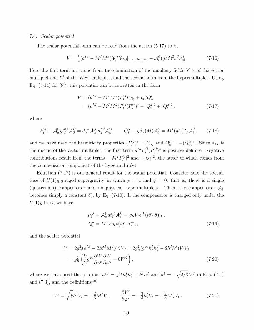
7.4. Scalar potential
The scalar potential term can be read from the action (5.17) to be
V = 14(aIJ −M IMJ )Y ij
I YJij|bosonic part −Aαi (gM)2
αβAi
β. (7.16)
Here the first term has come from the elimination of the auxiliary fields Y Iij of the vector
multiplet and tij of the Weyl multiplet, and the second term from the hypermultiplet. Using
Eq. (5.14) for Y ijI , this potential can be rewritten in the form
V = (aIJ −M IMJ)P ijI PJij +Qα
i Qiα
= (aIJ −M IMJ)P ijI (P ij
J )∗ − |Qai |2 + |Qα
i |2 , (7.17)
where
P ijI ≡ A(i
αgtαβI Aj)
β = dγαA(i
αgtγβI Aj)
β , Qαi ≡ gδG(M)Aα
i = M I(gtI)α
βAβi , (7.18)
and we have used the hermiticity properties (P ijI )∗ = PIij and Qi
α = −(Qαi )∗. Since aIJ is
the metric of the vector multiplet, the first term aIJP ijI (P ij
J )∗ is positive definite. Negative
contributions result from the terms −|M IP ijI |2 and −|Qa
i |2, the latter of which comes from
the compensator component of the hypermultiplet.
Equation (7.17) is our general result for the scalar potential. Consider here the special
case of U(1)R-gauged supergravity in which p = 1 and q = 0; that is, there is a single
(quaternion) compensator and no physical hypermultiplets. Then, the compensator Aai
becomes simply a constant δai , by Eq. (7.10). If the compensator is charged only under the
U(1)R in G, we have
P ijI = A(i
a gtabI Aj)
b = gRVIǫjk(i~q · ~σ)i
k ,
Qai = M IVIgR(i~q · ~σ)a
i , (7.19)
and the scalar potential
V = 2g2R(aIJ − 2M IMJ )VIVJ = 2g2
R(gxyhIxh
Jy − 2hIhJ)VIVJ
= g2R
(9
2gxy ∂W
∂ϕx
∂W
∂ϕy− 6W 2
), (7.20)
where we have used the relations aIJ = gxyhIxh
Jy + hIhJ and hI = −
√2/3M I in Eqs. (7.1)
and (7.3), and the definitions 16)
W ≡√
23h
IVI = −23M
IVI ,∂W
∂ϕx= −2
3hIxVI = −2
3MI,xVI . (7.21)
29

This agrees with the result by GST. 5) If the physical vector multiplets are not contained in
the system, the scalars ϕx do not appear either, and only the graviphoton with I = 0 exists.
In this case N = c000α3, and α = M I=0 is determined to be
√3/2 by the normalization
requirement of the graviphoton kinetic term, a00 = 1. Then, W = −√
2/3V0, and hence the
potential further reduces to
V = −4g2RV
20 , (7.22)
which agrees with the well-known anti-de Sitter cosmological term in the pure gauged su-
pergravity. 2)
§8. Conclusion and discussion
In this paper, we have presented an action for a general system of Yang-Mills vector
multiplets and hypermultiplet matter fields coupled to supergravity in five dimensions. The
supersymmetry transformation rules were also found. We have given these completely in
the off-shell formulation, in which all the auxiliary fields are retained. Our work can be
considered an off-shell extension of the preceding work by GST 5) and its generalization by
Ceresole and Dall’Agata. 6) [The latter authors also included ‘tensor multiplet matter fields’
(linear multiplets, in our terminology) with regard to which our system is less general.]
We have several applications in mind, such as compactifying on the orbifold S1/Z2 and/or
adding D-branes to the system. Then, the power of the present off-shell formulation will
become apparent. In particular, for the case of S1/Z2, it should be straightforward to
determine how to couple the bulk fields to the fields on the boundary planes, since we can
follow the general algorithm given by Mirabelli and Peskin for the case of the bulk Yang-Mills
supermultiplet. 7) Indeed, this program has been started very recently by Zucker 17) using his
off-shell formulation. He used a ‘tensor multiplet’ (linear multiplet) as a compensator for
the five-dimensional (pure) supergravity and found that the 4D supergravity induced on the
boundaries is a non-minimal version of N = 1 Poncare supergravity with 16+16 components
containing one auxiliary spinor, which was presented by Sohnius and West long ago. 18) This
non-minimal version is related to the new minimal version by the same authors. 19) Another
version of N = 1 Poncare supergravity, which is related to the usual minimal version, 20) will
appear if we start with our 5D supergravity in which the compensator is a hypermultiplet.
Adding D-branes in the system is not so straightforward. First of all, a D-brane is a
dynamical object whose position Xµ(x) in the bulk and its fermionic counterpart become a
supermultiplet in 4D that realizes the bulk (local) supersymmetry non-linearly. The problem
of identifying a supersymmetry transformation law for this multiplet and writing an invariant
30

action is already quite non-trivial, even in the case of rigid supersymmetry, and has long been
studied by several authors. 21) Once this problem is settled, coupling the bulk supergravity
to the fields on the D-brane should be easy also in this case. The off-shell formulation is
essential in any case.
Acknowledgements
The authors would like to thank Andre Lukas, Hiroaki Nakano, Paul Townsend, Antoine
Van Proeyen, Bernard de Wit and Max Zucker for discussions and useful information. They
also appreciate the Summer Institute 2000 held at Fuji-Yoshida, at which a preliminary
version of this work was reported. T. K. is supported in part by a Grant-in-Aid for Scientific
Research (No. 10640261) from the Japan Society for the Promotion of Science and a Grant-in-
Aid for Scientific Research on Priority Areas (No. 12047214) from the Ministry of Education,
Science, Sports and Culture, Japan.
31

Appendix A
A Representation Realizing Eq. (2.13)
The following is an example of the set of hermitian matrices TI, realizing the property
(2.13).
Let us prepare a representation vector ψi for each simple factor group Gi in G that gives
a faithful representation Ri of Gi, and a suitable numbers of singlet vectors ψα. Assigning
to them suitable U(1)x charges also, we consider a representation of G whose representation
vector is given by ψj , ψα, which transforms as follows under G =∏
iGi ×∏
x U(1)x:
under Gi U(1)x charges
ψj repr. Rj for i = j and singlet for i 6= j qxj
ψα singlet qxα
Let Ai be the generator label of the simple factor group Gi, ai be the component label of
the dimRj vector ψj = (ψai
j ), and ρRi(tAi
) = (ρRi(tAi
)aibi) be the representation matrices of
the generators acting on ψi in the representation Ri. Then the generators tI = (tAi, tx) of G
are given in this representation by
tAi
ajbj
= δijρRi(tAi
)aibi, tAi
αβ = 0,
txaj
bj= iδ
aj
bjqxj , tx
αβ = iδα
β qxα. (A.1)
The desired matrices TI are given by TAi= citAi
/i and Tx = tx/i. Equations given by (2.13)
to be satisfied are
G3i : 6cAiBiCi
= −ic3i tr(ρRi
(tAi)ρRi
(tBi), ρRi
(tCi)),
G2iU(1)x : 3cAiBix = −c2i qx
i tr(ρRi
(tAi)ρRi
(tBi)),
U(1)xU(1)yU(1)z : 3cxyz =∑
i
qxi q
yi q
zi dimRi +
∑
α
qxαq
yαq
zα.
The constants ci and U(1)x charges qxi of ψi are fixed by the first and second equations,
respectively. The third equation should be satisfied by adjusting the U(1)x charges qxα of ψα.
Clearly, there are such solutions for qxα if there are sufficiently many ψα.
Appendix B
U(2, n)/U(2) × U(n) as a Hypermultiplet Manifold for p = 2
In this appendix we explain how the manifold U(2, n)/U(2) × U(n) appears as a target
space manifold MQ of the physical hypermultiplet scalar fields for the case p = 2. This
32

is merely a detailed version of what was essentially shown long ago by Breitenlohner and
Sohnius. 14)
We consider the hypermultiplet Aαi in the standard representation, in which the matrices
dαβ and ραβ take the form 11)
dαβ =
(12p
−12q
), ραβ = ραβ =
ǫ
ǫ. . .
. (ǫ ≡ iσ2) (B.1)
The hypermultiplet Aαi is regarded as the 2(p+ q) × 2 matrix
A =
Aαi
=
...A2a−1,1 A2a−1,2
A2a,1 A2a,2...
, (a = 1, 2, · · · , p+ q) (B.2)
which consists of p+ q 2 × 2-blocks. Each block can be identified with a quaternion, which
is also mapped equivalently to a 2 × 2 matrix:
q ≡ q0 + iq1 + jq2 + kq3 ↔ q012 − i~q · ~σ =
(q0 − iq3 −iq1 − q2
−iq1 + q2 q0 + iq3
). (B.3)
This is consistent with the hermiticity condition for the hypermultiplet:
(Aαi)∗ = Aαi = ραβǫijAβj , → A† = −ǫATρ . (B.4)
The group G transformation and SU(2) U transformation act on A as
A → A′ = gAu†, g ∈ G, u ∈ SU(2). (B.5)
The G invariance of the quadratic form
AαidαβAβj ↔ A†dA = −ǫATρdA (B.6)
requires that the two conditions for g ∈ G,
g†d g = d, gTρd g = ρd , (B.7)
be satisfied. The former implies g ∈ U(2p, 2q) and the latter g ∈ Sp(2p+2q; C), so that the
group G must be a subgroup of USp(2p, 2q) = U(2p, 2q) ∩ Sp(2p+ 2q; C).
Now we consider the case p = 2, in which we gauge the U(1) group, which acts on A as
a phase rotation eiθ for the odd rows and as e−iθ for the even rows; that is, the generator is
given by T3 = σ3 ⊗ 1p+q. We do not give a kinetic term for the vector multiplet V3 coupling
33

to this charge T3. Then, the auxiliary field component Y ij3 of this multiplet appears only
in a linear form in the action: 2Y3ijAαidα
βT3βγAγj = 2 tr(Y3A†d T3A). Thus it acts as a
multiplier to impose the following three constraints on the hypermultiplet on-shell:
tr(σaA†d T3A) = 0 for a = 1, 2, 3. (B.8)
Moreover, we have one more constraint on-shell,
tr(A†dA) = 2 , (B.9)
which comes from the equation of motion A2 = −2N and the D gauge fixing condition
N = 1. Recall that we have two quaternion compensators for the present p = 2 case. Hence
there are eight (real) scalar fields with negative metric which should be eliminated. The
above constraints eliminate four components, and we still have SU(2) U symmetry acting
on the index i and the U(1) gauge symmetry for the charge T3. We can eliminate the
remaining four negative metric components by the gauge-fixing of these gauge symmetries,
so that the theory is consistent.
The manifold of the hypermultiplet specified by these four constraints (B.8) and (B.9)
have dimension 4(p + q) − 4 = 4 + 4q, and it is seen to be U(2, q)/U(2) × U(q) as follows.
First, we find that a representative element of A satisfying these constraints is given by
Arepr =1√2
12
iσ2
02...
02
. (B.10)
Second, to identify the manifold, it is sufficient to consider the half size (p+ q)× 2 complex
matrix Aodd that consists of the odd rows of A alone, since the even row elements are
essentially the complex conjugates of the odd row elements, as stipulated by the reality
condition of A. In this half-size representation, we can see that unitary transformations of
the above representative element,
Aodd = UAreprodd =
1√2U
1 0
0 1
0 0...
0 0
, U ∈ U(p, q), (B.11)
all satisfy the above constraints. But here, the subgroup U(q) ⊂ U(p, q) rotating the lower
q rows alone is inactive, so that the manifold of Aodd given by this form is U(p, q)/U(q) and
34

has dimension (p+ q)2 − q2 = p2 +2pq. However, when p = 2, this dimension already equals
the above dimension 4q + 4 for the hypermultiplet A specified by the constraints (B.8) and
(B.9), and thus the manifold of the latter is proved to be U(2, q)/U(q).
The manifold of the physical hypermultiplets is further reduced by the gauge fixing of
SU(2) and U(1), and hence becomes U(2, q)/U(q) × U(2).
Note also that the gauge group G is reduced to a subgroup of U(p, q) as a result of
the gauging of U(1). Indeed, the gauge transformation g ∈ G, compatible with the U(1)
symmetry, should commute with the U(1) generator T3: gT3 = T3g. One can easily see that
the group element g in USp(2p, 2q) satisfying this condition further must have the form
g =
(U 0
0 UT−1
), on
( Aodd
Aeven
)U ∈ U(p, q). (B.12)
This element clearly belongs to U(p, q).
References
[1] E. Cremmer, in Superspace and Supergravity, ed. S. Hawking and M. Rocek (Cam-
bridge University Press, 1980).
A. H. Chamseddine and H. Nicolai, Phys. Lett. B96 (1980), 89.
[2] R. D’Auria, P. Fre’, E. Maina and T. Regge, Ann. of Phys. 135 (1981), 237.
[3] E. Witten, Nucl. Phys. B471 (1996), 135, hep-th/9602070.
T. Banks and M. Dine, Nucl. Phys. B479 (1996), 173, hep-th/9605136.
[4] A. Lukas, B. A. Ovrut, K. S. Stelle and D. Waldram, Phys. Rev. D59 (1999), 086001,
hep-th/9803235; Nucl. Phys. B552 (1999), 246, hep-th/9806051.
[5] M. Gunaydin, G. Sierra and P. K. Townsend, Nucl. Phys. B242 (1984), 244; B253
(1985), 573.
[6] A. Ceresole and G. Dall’Agata, Nucl. Phys. B585 (2000), 143, hep-th/0004111.
[7] E. A. Mirabelli and M. E. Peskin, Phys. Rev. D58 (1998), 065002, hep-th/9712214.
[8] M. Zucker, Nucl. Phys. B570 (2000), 267, hep-th/9907082; hep-th/9909144.
[9] T. Kugo and K. Ohashi, Prog. Theor. Phys. 104 (2000), 835, hep-ph/0006231.
[10] E. Bergshoeff, E. Sezgin and A. Van Proeyen, Nucl. Phys. B264 (1986), 653.
[11] B. de Wit, P. G. Lauwers and A. Van Proeyen, Nucl. Phys. B255 (1985), 569.
[12] T. Kugo and S. Uehara, Nucl. Phys. B222 (1983), 125.
[13] B. de Wit, J. W. van Holten and A. Van Proeyen, Nucl. Phys. B167 (1980), 186;
B172 (1980), 543; B184 (1981), 77; B222 (1983), 516.
M. de Roo, J. W. van Holten, B. de Wit and A. Van Proeyen, Nucl. Phys. B173
35

(1980), 175.
E. Bergshoeff, M. de Roo and B. de Wit, Nucl. Phys. B182 (1981), 173.
[14] P. Breitenlohner and M. F. Sohnius, Nucl. Phys. B187 (1981), 409.
[15] H. Nishino and E. Sezgin, Trieste Preprint IC/84/50.
B. de Wit and A. Van Proeyen, Nucl. Phys. B245 (1984), 89.
[16] E. Bergshoeff, R. Kallosh and A. Van Proeyen, J. High Energy Phys. 10 (2000),
033, hep-th/0007044.
[17] M. Zucker, hep-th/0009083.
[18] M. F. Sohnius and P. C. West, Nucl. Phys. B216 (1983), 100.
[19] M. F. Sohnius and P. C. West, Phys. Lett. 105B (1981), 353.
[20] K. S. Stelle and P. C. West, Phys. Lett. 74B (1978), 330.
S. Ferrara and P. van Niewenhuizen, Phys. Lett. 74B (1978), 333.
[21] J. Bagger and J. Wess, Phys. Lett. B138 (1984), 105.
J. Hughes and J. Polchinski, Nucl. Phys. B278 (1986), 147.
J. Bagger and A. Galperin, Phys. Lett. B336 (1994), 25, hep-th/9707061;
Phys. Rev. D55 (1997), 1091, hep-th/9608177; Phys. Lett. B412 (1997), 296,
hep-th/9707061.
I. Antoniadis, H. Partouche and T. R. Taylor, Phys. Lett. B372 (1996), 83, hep-
th/9512006.
S. Ferrara, L. Girardello and M. Porrati, Phys. Lett. B376 (1996), 275,
hep-th/9512180.
M. Rocek and A. A. Tseytlin, Phys. Rev. D59 (1999), 106001, hep-th/9811232.
36