o nonlinear dynamics and chaos - henri menke · fp v41 (2015) fortgeschrittenenpraktikum january...

FP V41 (2015) FORTGESCHRITTENENPRAKTIKUM January 19, 2015

o

Nonlinear Dynamics and Chaos

Michael Schmid∗ and Henri Menke†

(January 19, 2015)

The present experiment deals with the fundamental properties of nonlinear dynamical systems,chaotic behaviour and chaos. In the experiment two different kinds of nonlinear oscillators areinvestigated, viz. the inverted pendulum and a Shinriki oscillator. To find chaotic behaviour andperiodic orbits the phase portrait, autocorrelation function as well as the Fourier transform of themeasured signal are calculated. In case of the Shinriki oscillator a Feigenbaum diagram and a phasediagram of the control parameter is recorded.

BASICS

The following section is a short introduction to non-linear dynamical systems, chaos and their mathematicaldescription.

Dynamical Systems

For many physical problems it is possible to rewritethe equations of motion in a set of first order differentialequation

d

dtx(t) = F (x(t), t), (1)

where t is the time, x(t) the trajectory in real spaceand F (x(t), t) a vector field. Note that F (x(t), t) is ingeneral a smooth function. The whole time evolution of adynamical system is determined by the initial conditionsand hence it is always possible to find a deterministicsolution. A more formal definition is:

Definition 1 (from [1]). A smooth dynamical system onRn is a continuously differentiable function φ : R×Rn →Rn, where φ(t,x) = φt(x) satisfies

1. φ0 : Rn → Rn is the identity function: φ0(x0) = x0.

2. The composition φt φs = φt+s for each t, s ∈ R.

Here φt(x) is the so called evolution function or flowwhich describes how the system in the configuration xevolves in time t. If F (x(t)) does not explicitly depend ont we deal with a so called autonomous systems. Calcula-tion of an analytical solution in case of nonlinear systemsis rarely feasible. A physical system is called nonlinearif additional time dependent variables of higher ordersappear in equation (1). Typical examples of nonlinearsystems are damped driven pendulums, the three bodyproblem or the Navier-Stokes equation [1, 2].

Phase Space: All possible states of a dynamical systemare represented in the phase space which consists of allconceivable values of space and momentum variables and

is therefore a vector space. A more formal representationis given by the phase space vector

ξ =(q1, . . . , qf , p1, . . . , pf

)T, (2)

where qi are the positions, pi the corresponding momentaand f the number of degrees of freedom [3].

Dissipative Systems: In the case of Hamiltonian sys-tems the phase space distribution function is constantalong the trajectories of the system according to Liou-ville’s theorem, i.e. the phase space volume is preserved.If the systems contains additional dissipative terms thephase space volume decreases and the system is calleddissipative. A typical example is a damped harmonicoscillator.

Trajectories in the phase space must not intersect, oth-erwise the intersection point leads to indefinite time evolu-tion. Note that nonlinear dynamical systems may exhibitchaotic behaviour, which is in general not equivalent tochaos.

Chaos

Dynamical systems that are highly sensitive to initialconditions may contain chaotic behaviour or chaos, i.e.small differences in the initial conditions results in dif-ferent outcomes. Therefore a long term prediction is ingeneral impossible. Although these systems are deter-ministic it is not possible to predict their future. Thisbehaviour is called deterministic chaos. Typical examplesare the three body problem or the Lorenz attractor.

Lyapunov Exponent: To describe the evolution be-haviour of a dynamical system it is common to define theLyapunov exponent

λi = limt→∞

1

tln

(‖δxi(t)‖‖δxi0‖

), (3)

where the index i describes the spatial direction, ‖δxi(t)‖the distance between the i-th component of the observedcurve and the reference curve at time t and ‖δxi0‖ thedistance at time 0. The Lyapunov exponent is a measure

1


for the rate of separation of infinitesimally close trajec-tories. For λ > 0 the trajectories diverge, for λ < 0 theyconverge. The distance remains constant if λ = 0.

Attractor: An attractor describes the long time evo-lution of a dynamical system for a wide variety of initialconditions, i.e. a set of points in phase space towards thesystem contracts. Once an attractor is reached it is impos-sible to leave it. An attractor can be a single point (or afinite set of non-continuously distributed points), a curve(limit cycle), a manifold (torus) or a strange attractor likethe Lorenz attractor.

Signal Analysis and Autocorrelation

This section shows how to identify important propertiesof a dynamical system by Fourier transform the measuredsignal, looking at the autocorrelation function or thepower spectral density. Henceforth the notation x(t) isused for the measured signal.

Fourier Transformation: The Fourier transformationof a function f(t) is given by

F(ω) ≡ 1√2π

∞∫−∞

f(t)e−iωt dt. (4)

The inverse Fourier transformation is

f(t) ≡ 1√2π

∞∫−∞

F(ω)eiωt dω. (5)

Note that f(t) is an integrable function.

Autocorrelation: The autocorrelation function γ(τ) isdefined by

γ(τ) ≡ 〈x(t), x(t+ τ)〉 (6)

=

∞∫−∞

x(τ)x(t+ τ) dτ (7)

and is a tool for finding repeating pattern like periodicbehaviour. In case of chaotic behaviour the autocorrela-tion function is zero. For periodic behaviour one observesan autocorrelation function much larger than zero. Notethat a measurement process itself is finite in time andtherefore it is not possible to integrate from −∞ to ∞and the total energy can not reach a finite value. Is thisthe case it is helpful to use the time average

γ(τ) ≡ limT→∞

1

2T

T∫−T

x(t+ τ)x(t) dt, (8)

where T is the period time.

Power Spectral Density: The power spectral density(PSD) describes the optical power per frequency intervaland has the physical dimension [PSD] = W Hz−1. We canalso say it describes how the power of signal or time seriesare disturbed over different frequencies. It is defined by

Sxx ≡∫ ∞−∞

γ(τ)e−iωτ dτ, (9)

where γ(τ) = 〈x(t), x(t+ τ)〉 is the autocorrelation func-tion of the measured signal. The PSD is a statisticalmeasure which can be calculated by averaging over manymeasurement results.

Discret Dynamical Systems

Sometimes it is possible to reduce a differential equationto an iterated function. Due to the lower dimensionalspace a easier visualisation is possible. Moreover insteadof integrating it is now possible to solve the problem byiterating the function over and over. An iterative functionin one dimension is given by the map

ui 7→ ui+1 = f(ui). (10)

A point is called a fixed point if u(x0) = x0. A periodicpoint of period n is given by un(x0) = x0 for some n > 0.As a consequence a periodic orbit repeats itself. A periodicpoint x0 has minimal period n if n is the least positiveinteger for which un(x0) = x0 [1, 2].

Logistic Map: A typical example of a discrete dynam-ical system is the logistic map

xn+1 = rxn(1− xn), (11)

where r > 0 is a control parameter and x ∈ [0, 1]. Thelogistic map is a mathematical model for a driven dampedoscillator. Plotting x over r for many iterations one hasthe so called Feigenbaum diagram, cf. figure 1 whichallows the determination of the Feigenbaum constants δand α. The constant δ is given by the ratio of the lengthof two following periodic windows

δ =rn−1 − rn−2rn − rn−1

≈ 4.6692. (12)

The constant α is given by the ratio of the width of twofollowing periodic windows.

α ≈ 2.5029. (13)

ANALYSIS

In this section we discuss the experimental proceduresand the analysis of the measured data.

2


0.1

0.2

0.3

0.4

0.5

0.6

0.7

0.8

0.9

1

2.6 2.8 3 3.2 3.4 3.6 3.8 4

x

r

FIG. 1. Feigenbaum diagram. The logistic map for manyiterations is shown.

Experimental Task and Setup

The experiment is mainly divided into four experimen-tal tasks.

Inverted Pendulum: With help of a computer softwarethe displacement and velocity are measured as a functionof time to investigate the phase diagram and the Fouriertransform of the displacement. Measurements were donefor different driving frequencies. The aim is to observeorbits with period one, two or higher, as well as chaoticbehaviour.

Shinriki-Oscillator: Like in the previous task measure-ments were done with help of a computer software toobserve different vibrational states. This time the resis-tances R1 and R2 are the control parameters. It is onlyallowed to vary these parameters.

Feigenbaum diagram: For creating a Feigenbaum di-agram it is necessary to do a lot of measurements forvarying control parameter R1. By plotting just the max-ima of the measured data, i.e. the voltage as functionof the control parameter R1 a wild Feigenbaum diagramappears. With help of the diagram it is then possible todetermine the Feigenbaum constant δ.

Phase diagram: With help of the Shinriki oscillator itis possible to create a phase diagram of the two controlparameters R1 and R2. Therefore the measurement hadto be done by varying one of the control parameters whilethe other one is held constant and vice versa. While oneof the control parameters is varied the transitions betweendifferent vibrational states are noted down.

The experimental setup of the inverted pendulum isdepicted in figure 2 and the Shinriki oscillator in figure 3.The data were recorded with LabVIEW.

FIG. 2. Circuit diagram of the inverted pendulum.

FIG. 3. Circuit diagram of a Shinriki oscillator. R1 and R2

are the control parameters.

Inverted Pendulum

The following experimental task deals with the invertedpendulum. Before it is possible to record measurementsthe experimental setup had to be adjusted. We chose forthe oscillating mass two small copper discs and two smallmetal discs. The springs were applied at an altitude of7 cm. All subsequent measurements were done with thisadjustment.

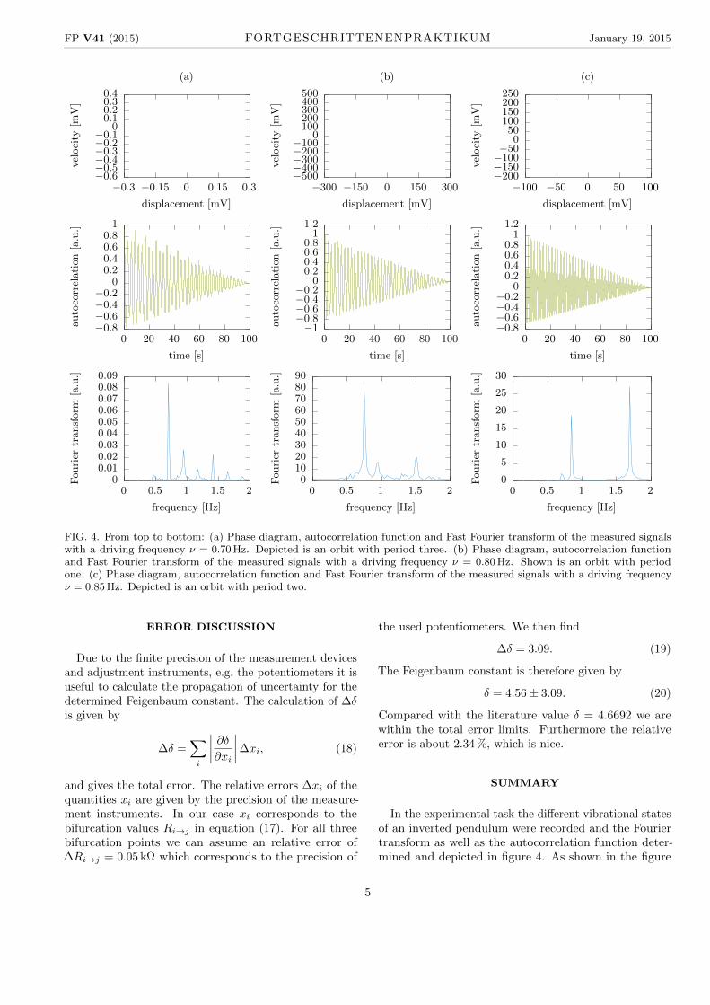
By varying the driving frequency it was possible toobserve different vibrational sates. To identify them theautocorrelation function (8) and the Fourier transform (4)of the measured signal were calculated with python. Forpresent adjustment it was possible to identify the followingvibrational states:

• An orbit with period three as shown in figure 4 (a).With help of the Fourier transformed signal thisidentification is possible. Obviously there are threeresonance frequencies besides the driving frequencyν = 0.7 Hz. There are also higher orders visible inthe figure.

• An Orbit with period one as depicted in figure 4 (b).This corresponds to the high resonance peak nearthe driving frequency 0.80 Hz. This can also be seenin the decreasing autocorrelation function.

3


• An orbit with period two as depicted in figure 4 (c).In the autocorrelation function it is possible to ob-serve two decreasing oscillations. The two reso-nance frequencies are also visible in the Fouriertransformed signal.

One can see that it is possible to identify the reso-nance frequencies in the Fourier transformed figures. Theautocorrelation function decays for all measurements tozero. As discussed in the basics this is due to the finitemeasurement time.

Shinriki Oscillator

Like in the previous experimental task we are now in-terested in observing different vibrational states. Insteadof varying the driving frequency now the two control re-sistances R1 and R2 are varied. For the measurementsshown in figure 7 the resistance R2 = 18.6 kΩ while R1 isvaried. The measurements were done with a LabVIEWprogram. The analysis is the same as in the previous task.The measured data and the corresponding autocorrelationfunctions as well as the Fourier transforms are depictedin figure 7.

With help of the figure it is possible to identify thefollowing vibrational states:

• An orbit with period one is depicted in figure 7 (a).The autocorrelation function decreases continuallyand no other oscillations are superimposed.

• An orbit with period two is shown in figure 7 (b)and (f). The autocorrelation functions shows this.The Fourier transformed signal shows two peakscorresponding to the resonance frequencies.

• An orbit with period three is depicted in figure 7(e). All three resonances are visible in the Fouriertransformed signal.

• An orbit with period four is given in 7 (c). TheFourier transformed signal shows all four peakswhere two of them are dominant compared to theothers.

• Mono-scroll chaos was observed in figure 7 (d). TheFourier transformed signal shows the chaotic be-haviour. One dominant peak surrounded by noiseis visible.

• Double-scroll chaos is depicted in figure 7 (g). Obvi-ously the autocorrelation function shows that thereis no correlation in the signal. The two peaks in theFourier transformed signal are surrounded by noise.

Feigenbaum Diagram

For the Shinriki oscillator it is possible to observe aFeigenbaum diagram by doing a lot of measurements.Therefore we choose the control parameter R2 = 9.3 kΩand varied R1. For each varied R1 the measurement isrecorded. By searching the maximum of the recordeddata a data point to the adjusted R1 for the Feigenbaumdiagram is found. Plotting all these data one has theFeigenbaum diagram depicted in figure 5. To determinethe Feigenbaum constant δ it is necessary to find thedata points which correspond to a bifurcation point. Anumerical search yields

R1→2 = 16.80 kΩ, (14)

R2→4 = 17.62 kΩ, (15)

R4→8 = 17.80 kΩ. (16)

The subscript in Ri→j indicates that for this controlparameter a change from period i to period j occurs.Note that the figure shows only an interval of R1 wherea valid analysis is possible. With the bifurcation pointsthe determination of the Feigenbaum constant is possible.For the measured data we find

δ =R2→4 −R1→2

R4→8 −R2→4= 4.56. (17)

The literature value is δ = 4.6692.

Phase Diagram

To record a phase diagram of the control parametersR1 and R2 it is necessary to hold first one of the controlparameter constant while the other one is varied. Weheld R2 fixed and varied then R1 from 0 kΩ to 100 kΩ andnoted down the points where a change of the vibrationalstate is observed. Then a new value for R2 is chosenand the measurement process is repeated. The measureddata were then plotted in a phase diagram to identify theparameter constellations were different vibrational statesare possible. The diagram is depicted in figure 6. Thefigure shows that for high values of R2 it is possible toend at a great orbit with period one. Once this orbit isreached it is impossible to go backwards, i.e. we end on anattractor. Also for small values of R2 it is only possible toobserve an orbit of period one. Nevertheless, as depictedfor greater values of R2, it is possible to observe nearlyall vibrational states discussed in figure 7. Note thatfor some cases it was due to the finite precision of thepotentiometer a bit annoying to identify the correct orbits.Moreover the figure shows that double-scroll chaos andmono-scroll chaos appear very often.

4


−0.6−0.5−0.4−0.3−0.2−0.1

00.10.20.30.4

−0.3 −0.15 0 0.15 0.3

vel

oci

ty[m

V]

displacement [mV]

(a)

−0.8−0.6−0.4−0.2

00.20.40.60.8

1

0 20 40 60 80 100

auto

corr

elati

on

[a.u

.]

time [s]

00.010.020.030.040.050.060.070.080.09

0 0.5 1 1.5 2

Fouri

ertr

ansf

orm

[a.u

.]

frequency [Hz]

−500−400−300−200−100

0100200300400500

−300 −150 0 150 300

vel

oci

ty[m

V]

displacement [mV]

(b)

−1−0.8−0.6−0.4−0.2

00.20.40.60.8

11.2

0 20 40 60 80 100

auto

corr

elati

on

[a.u

.]

time [s]

0102030405060708090

0 0.5 1 1.5 2

Fouri

ertr

ansf

orm

[a.u

.]

frequency [Hz]

−200−150−100−50

050

100150200250

−100 −50 0 50 100

vel

oci

ty[m

V]

displacement [mV]

(c)

−0.8−0.6−0.4−0.2

00.20.40.60.8

11.2

0 20 40 60 80 100

auto

corr

elati

on

[a.u

.]

time [s]

0

5

10

15

20

25

30

0 0.5 1 1.5 2

Fouri

ertr

ansf

orm

[a.u

.]

frequency [Hz]

FIG. 4. From top to bottom: (a) Phase diagram, autocorrelation function and Fast Fourier transform of the measured signalswith a driving frequency ν = 0.70 Hz. Depicted is an orbit with period three. (b) Phase diagram, autocorrelation functionand Fast Fourier transform of the measured signals with a driving frequency ν = 0.80 Hz. Shown is an orbit with periodone. (c) Phase diagram, autocorrelation function and Fast Fourier transform of the measured signals with a driving frequencyν = 0.85 Hz. Depicted is an orbit with period two.

ERROR DISCUSSION

Due to the finite precision of the measurement devicesand adjustment instruments, e.g. the potentiometers it isuseful to calculate the propagation of uncertainty for thedetermined Feigenbaum constant. The calculation of ∆δis given by

∆δ =∑i

∣∣∣∣ ∂δ∂xi∣∣∣∣∆xi, (18)

and gives the total error. The relative errors ∆xi of thequantities xi are given by the precision of the measure-ment instruments. In our case xi corresponds to thebifurcation values Ri→j in equation (17). For all threebifurcation points we can assume an relative error of∆Ri→j = 0.05 kΩ which corresponds to the precision of

the used potentiometers. We then find

∆δ = 3.09. (19)

The Feigenbaum constant is therefore given by

δ = 4.56± 3.09. (20)

Compared with the literature value δ = 4.6692 we arewithin the total error limits. Furthermore the relativeerror is about 2.34 %, which is nice.

SUMMARY

In the experimental task the different vibrational statesof an inverted pendulum were recorded and the Fouriertransform as well as the autocorrelation function deter-mined and depicted in figure 4. As shown in the figure

5


0

0.5

1

1.5

2

2.5

16 16.5 17 17.5 18 18.5 19 19.5 20

Volt

age

[V]

Resistance R1 [kΩ]

FIG. 5. Feigenbaum diagram of the Shinriki oscillator for fixedR2 = 9.3 kΩ and varying R1.

0

20

40

60

80

100

0 5 10 15 20

Res

ista

nceR

1[k

Ω]

Resistance R2 [kΩ]

Period 1 Mono-scroll ChaosPeriod 2 Double-scroll ChaosPeriod 3 Great OrbitPeriod 4

FIG. 6. Phase diagram of the Shinriki oscillator. Depicted isR1 as function of R2. The areas where different vibrationalstates are possible are coloured.

it was possible to investigate orbits of period one, twoand three. The resonance peaks are given in the Fouriertransformed signal.

The same observations were done in the case of theShinriki oscillator as depicted in figure 7. Moreover it waspossible to create a Feigenbaum diagram 5 and determinethe Feigenbaum constant to

δ = 4.56± 3.09. (21)

Compared to the literature value δ = 4.6692 this cor-responds to a relative error of 2.34 %. Moreover it waspossible to observe a phase diagram 6 to identify thedifferent areas of vibrational states as function of the twocontrol parameters R1 and R2.

∗ Michael [email protected]† [email protected]

[1] M. W. Hirsch, S. Smale, and R. L. Devaney, Differentialequations, dynamical systems, and an introduction to chaos,3rd ed. (Academic press, 2013).

[2] F. Scheck, Theoretische Physik 1: Mechanik, 8th ed.(Springer, 1999).

[3] U. Seifert, Theoretische Physik 1, 1st ed. (UniversitatStuttgart, 2012).

6


−1.2

−0.6

0

0.6

1.2

−1.5−1 −0.5 0 0.5 1 1.5

U2

[V]

U1 [V]

(a)

(b)

(c)

(d)

(e)

(f)

(g)

−1.2

−0.6

0

0.6

1.2

0 20 40

AC

Fγ

[a.u

.]

time [s]

0

0.4

0.8

1.2

0 0.2 0.4 0.6 0.8 1

FF

TF

[a.u

.]

frequency [kHz]

−1.2

−0.6

0

0.6

1.2

−2 −1 0 1 2

U2

[V]

U1 [V]

−1.2

−0.6

0

0.6

1.2

0 20 40

AC

Fγ

[a.u

.]time [s]

0

0.4

0.8

1.2

0 0.25 0.5 0.75 1

FF

TF

[a.u

.]

frequency [kHz]

−1.2

−0.6

0

0.6

1.2

−2 −1 0 1 2

U2

[V]

U1 [V]

−1.2

−0.6

0

0.6

1.2

0 20 40

AC

Fγ

[a.u

.]

time [s]

0

0.4

0.8

1.2

0 0.25 0.5 0.75 1

FF

TF

[a.u

.]

frequency [kHz]

−1.2

−0.6

0

0.6

1.2

−2 −1 0 1 2 3

U2

[V]

U1 [V]

−1.2

−0.6

0

0.6

1.2

0 20 40

AC

Fγ

[a.u

.]

time [s]

0

0.4

0.8

1.2

0 0.25 0.5 0.75 1

FF

TF

[a.u

.]frequency [kHz]

−1.2

−0.6

0

0.6

1.2

−2 −1 0 1 2 3

U2

[V]

U1 [V]

−0.6

0

0.6

1.2

0 20 40

AC

Fγ

[a.u

.]

time [s]

0

0.4

0.8

0 0.25 0.5 0.75 1

FF

TF

[a.u

.]

frequency [kHz]

−1.8−1.2−0.6

00.61.21.8

−5−4−3−2−1 0 1 2 3 4 5

U2

[V]

U1 [V]

−1.2

−0.6

0

0.6

1.2

0 20 40

AC

Fγ

[a.u

.]

time [s]

00.40.81.21.6

22.4

0 0.25 0.5 0.75 1

FF

TF

[a.u

.]

frequency [kHz]

−1.8−1.2−0.6

00.61.21.8

−5 0 5

U2

[V]

U1 [V]

−0.6

0

0.6

1.2

0 20 40 60

AC

Fγ

[a.u

.]

time [s]

0

0.4

0.8

1.2

1.6

0 0.25 0.5 0.75 1

FF

TF

[a.u

.]

frequency [kHz]

FIG. 7. From left to right. Phase diagram, autocorrelation function and Fourier transform for: (a) Orbit of period onewith R1 = 16.0 kΩ, R2 = 18.6 kΩ. (b) Orbit of period two with R1 = 17.5 kΩ, R2 = 18.6 kΩ. (c) Orbit of period four withR1 = 17.8 kΩ, R2 = 18.6 kΩ. (d) Mono- scroll chaos for R1 = 18.5 kΩ, R2 = 18.6 kΩ. (e) Orbit of period three with R1 = 18.6 kΩ,R2 = 18.6 kΩ. (f) Orbit of period two with R1 = 28.8 kΩ, R2 = 18.6 kΩ. (g) Double-scroll chaos for R1 = 30.6 kΩ, R2 = 18.6 kΩ.

7

o nonlinear dynamics and chaos - henri menke · fp v41 (2015) fortgeschrittenenpraktikum january...

Documents