numericalmathematicsi - math.lmu.de
TRANSCRIPT

Numerical Mathematics I
Peter Philip∗
Lecture Notes
Originally Created for the Class of Winter Semester 2008/2009 at LMU Munich,
Revised and Extended for Several Subsequent Classes†
November 10, 2021
Contents
1 Introduction and Motivation 5
2 Tools: Landau Symbols, Norms, Condition 9
2.1 Landau Symbols . . . . . . . . . . . . . . . . . . . . . . . . . . . . . . . 9
2.2 Operator Norms and Natural Matrix Norms . . . . . . . . . . . . . . . . 16
2.3 Condition of a Problem . . . . . . . . . . . . . . . . . . . . . . . . . . . . 22
3 Interpolation 36
3.1 Motivation . . . . . . . . . . . . . . . . . . . . . . . . . . . . . . . . . . . 36
3.2 Polynomial Interpolation . . . . . . . . . . . . . . . . . . . . . . . . . . . 37
3.2.1 Polynomials and Polynomial Functions . . . . . . . . . . . . . . . 37
3.2.2 Existence and Uniqueness . . . . . . . . . . . . . . . . . . . . . . 40
3.2.3 Hermite Interpolation . . . . . . . . . . . . . . . . . . . . . . . . . 42
∗E-Mail: [email protected]†Resources used in the preparation of this text include [DH08, GK99, HB09, Pla10].
1

CONTENTS 2
3.2.4 Divided Differences and Newton’s Interpolation Formula . . . . . 50
3.2.5 Convergence and Error Estimates . . . . . . . . . . . . . . . . . . 58
3.2.6 Chebyshev Polynomials . . . . . . . . . . . . . . . . . . . . . . . . 60
3.3 Spline Interpolation . . . . . . . . . . . . . . . . . . . . . . . . . . . . . . 64
3.3.1 Introduction, Definition of Splines . . . . . . . . . . . . . . . . . . 64
3.3.2 Linear Splines . . . . . . . . . . . . . . . . . . . . . . . . . . . . . 67
3.3.3 Cubic Splines . . . . . . . . . . . . . . . . . . . . . . . . . . . . . 68
4 Numerical Integration 78
4.1 Introduction . . . . . . . . . . . . . . . . . . . . . . . . . . . . . . . . . . 78
4.2 Quadrature Rules Based on Interpolating Polynomials . . . . . . . . . . . 82
4.3 Newton-Cotes Formulas . . . . . . . . . . . . . . . . . . . . . . . . . . . 84
4.3.1 Definition, Weights, Degree of Accuracy . . . . . . . . . . . . . . 84
4.3.2 Rectangle Rules (n = 0) . . . . . . . . . . . . . . . . . . . . . . . 88
4.3.3 Trapezoidal Rule (n = 1) . . . . . . . . . . . . . . . . . . . . . . . 89
4.3.4 Simpson’s Rule (n = 2) . . . . . . . . . . . . . . . . . . . . . . . . 90
4.3.5 Higher Order Newton-Cotes Formulas . . . . . . . . . . . . . . . . 91
4.4 Convergence of Quadrature Rules . . . . . . . . . . . . . . . . . . . . . . 92
4.5 Composite Newton-Cotes Quadrature Rules . . . . . . . . . . . . . . . . 94
4.5.1 Introduction, Convergence . . . . . . . . . . . . . . . . . . . . . . 95
4.5.2 Composite Rectangle Rules (n = 0) . . . . . . . . . . . . . . . . . 97
4.5.3 Composite Trapezoidal Rules (n = 1) . . . . . . . . . . . . . . . . 98
4.5.4 Composite Simpson’s Rules (n = 2) . . . . . . . . . . . . . . . . . 99
4.6 Gaussian Quadrature . . . . . . . . . . . . . . . . . . . . . . . . . . . . . 99
4.6.1 Introduction . . . . . . . . . . . . . . . . . . . . . . . . . . . . . . 99
4.6.2 Orthogonal Polynomials . . . . . . . . . . . . . . . . . . . . . . . 100
4.6.3 Gaussian Quadrature Rules . . . . . . . . . . . . . . . . . . . . . 103
5 Numerical Solution of Linear Systems 108
5.1 Background and Setting . . . . . . . . . . . . . . . . . . . . . . . . . . . 108
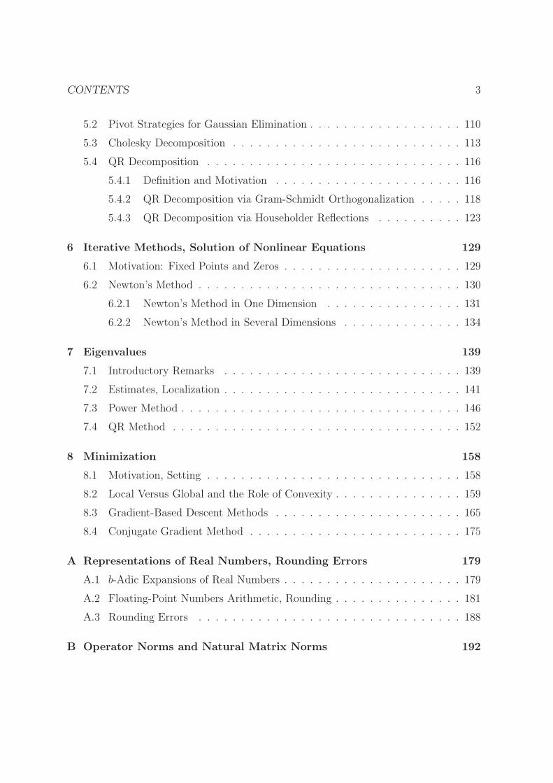
CONTENTS 3
5.2 Pivot Strategies for Gaussian Elimination . . . . . . . . . . . . . . . . . . 110
5.3 Cholesky Decomposition . . . . . . . . . . . . . . . . . . . . . . . . . . . 113
5.4 QR Decomposition . . . . . . . . . . . . . . . . . . . . . . . . . . . . . . 116
5.4.1 Definition and Motivation . . . . . . . . . . . . . . . . . . . . . . 116
5.4.2 QR Decomposition via Gram-Schmidt Orthogonalization . . . . . 118
5.4.3 QR Decomposition via Householder Reflections . . . . . . . . . . 123
6 Iterative Methods, Solution of Nonlinear Equations 129
6.1 Motivation: Fixed Points and Zeros . . . . . . . . . . . . . . . . . . . . . 129
6.2 Newton’s Method . . . . . . . . . . . . . . . . . . . . . . . . . . . . . . . 130
6.2.1 Newton’s Method in One Dimension . . . . . . . . . . . . . . . . 131
6.2.2 Newton’s Method in Several Dimensions . . . . . . . . . . . . . . 134
7 Eigenvalues 139
7.1 Introductory Remarks . . . . . . . . . . . . . . . . . . . . . . . . . . . . 139
7.2 Estimates, Localization . . . . . . . . . . . . . . . . . . . . . . . . . . . . 141
7.3 Power Method . . . . . . . . . . . . . . . . . . . . . . . . . . . . . . . . . 146
7.4 QR Method . . . . . . . . . . . . . . . . . . . . . . . . . . . . . . . . . . 152
8 Minimization 158
8.1 Motivation, Setting . . . . . . . . . . . . . . . . . . . . . . . . . . . . . . 158
8.2 Local Versus Global and the Role of Convexity . . . . . . . . . . . . . . . 159
8.3 Gradient-Based Descent Methods . . . . . . . . . . . . . . . . . . . . . . 165
8.4 Conjugate Gradient Method . . . . . . . . . . . . . . . . . . . . . . . . . 175
A Representations of Real Numbers, Rounding Errors 179
A.1 b-Adic Expansions of Real Numbers . . . . . . . . . . . . . . . . . . . . . 179
A.2 Floating-Point Numbers Arithmetic, Rounding . . . . . . . . . . . . . . . 181
A.3 Rounding Errors . . . . . . . . . . . . . . . . . . . . . . . . . . . . . . . 188
B Operator Norms and Natural Matrix Norms 192

CONTENTS 4
C Integration 195
C.1 Km-Valued Integration . . . . . . . . . . . . . . . . . . . . . . . . . . . . 195
C.2 Continuity . . . . . . . . . . . . . . . . . . . . . . . . . . . . . . . . . . . 197
D Divided Differences 198
E DFT and Trigonometric Interpolation 201
E.1 Discrete Fourier Transform (DFT) . . . . . . . . . . . . . . . . . . . . . . 201
E.2 Approximation of Periodic Functions . . . . . . . . . . . . . . . . . . . . 205
E.3 Trigonometric Interpolation . . . . . . . . . . . . . . . . . . . . . . . . . 209
E.4 Fast Fourier Transform (FFT) . . . . . . . . . . . . . . . . . . . . . . . . 213
F The Weierstrass Approximation Theorem 220
G Baire Category and the Uniform Boundedness Principle 223
H Matrix Decomposition 226
H.1 Cholesky Decomposition of Positive Semidefinite Matrices . . . . . . . . 226
H.2 Multiplication with Householder Matrix over R . . . . . . . . . . . . . . 230
I Newton’s Method 231
J Eigenvalues 233
J.1 Continuous Dependence on Matrix Coefficients . . . . . . . . . . . . . . . 233
J.2 Transformation to Hessenberg Form . . . . . . . . . . . . . . . . . . . . . 235
J.3 QR Method for Matrices in Hessenberg Form . . . . . . . . . . . . . . . . 239
K Minimization 243
K.1 Golden Section Search . . . . . . . . . . . . . . . . . . . . . . . . . . . . 243
K.2 Nelder-Mead Method . . . . . . . . . . . . . . . . . . . . . . . . . . . . . 248

1 INTRODUCTION AND MOTIVATION 5
1 Introduction and Motivation
The central motivation of Numerical Mathematics is to provide constructive and effectivemethods (so-called algorithms, see Def. 1.1 below) that reliably compute solutions (orsufficiently accurate approximations of solutions) to classes of mathematical problems.Moreover, such methods should also be efficient, i.e. one would like the algorithm tobe as quick as possible while one would also like it to use as little memory as possible.Frequently, both goals can not be achieved simultaneously: For example, one mightdecide to recompute intermediate results (which needs more time) to avoid storing them(which would require more memory) or vice versa. One typically also has a trade-off between accuracy and requirements for memory and execution time, where higheraccuracy means use of more memory and longer execution times.
Thus, one of the main tasks of Numerical Mathematics consists of proving that a givenmethod is constructive, effective, and reliable. That a method is constructive, effective,and reliable means that, given certain hypotheses, it is guaranteed to converge to thesolution. This means, it either finds the solution in a finite number of steps, or, moretypically, given a desired error bound, within a finite number of steps, it approximatesthe true solution such that the error is less than the given bound. Proving error esti-mates is another main task of Numerical Mathematics and so is proving bounds on analgorithm’s complexity, i.e. bounds on its use of memory (i.e. data) and run time (i.e.number of steps). Moreover, in addition to being convergent, for a method to be useful,it is of crucial importance that is also stable in the sense that a small perturbation ofthe input data does not destroy the convergence and results in, at most, a small increaseof the error. This is of the essence as, for most applied problems, the input data willnot be exact, and most algorithms are subject to round-off errors.
Instead of a method, we will usually speak of an algorithm, by which we mean a “useful”method. To give a mathematically precise definition of the notion algorithm is beyondthe scope of this lecture (it would require an unjustifiably long detour into the field oflogic), but the following definition will be sufficient for our purposes.
Definition 1.1. An algorithm is a finite sequence of instructions for the solution of aclass of problems. Each instruction must be representable by a finite number of symbols.Moreover, an algorithm must be guaranteed to terminate after a finite number of steps.
Remark 1.2. Even though we here require an algorithm to terminate after a finitenumber of steps, in the literature, one sometimes omits this part from the definition.The question if a given method can be guaranteed to terminate after a finite number ofsteps is often tremendously difficult (sometimes even impossible) to answer.
Example 1.3. Let a, a0 ∈ R+ and consider the sequence (xn)n∈N0 defined recursively
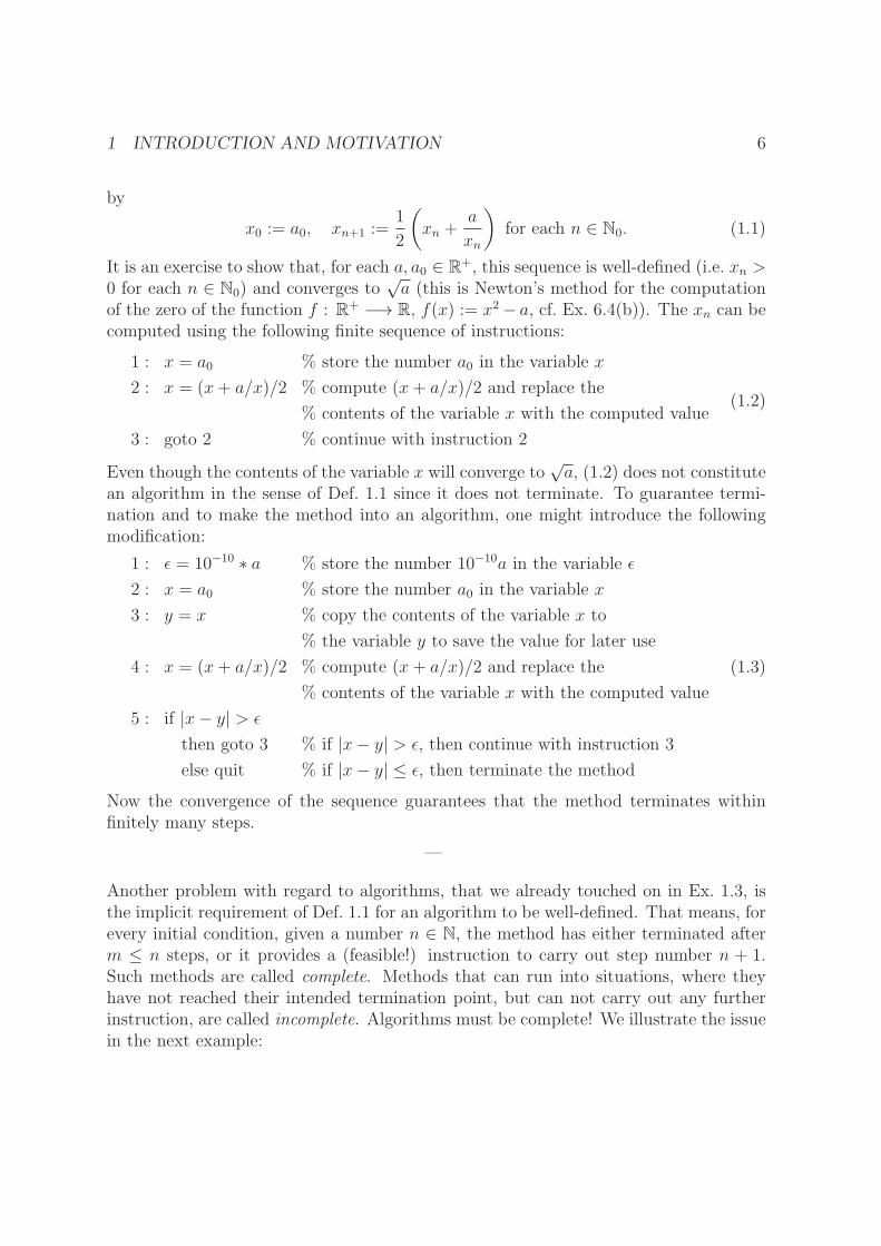
1 INTRODUCTION AND MOTIVATION 6
by
x0 := a0, xn+1 :=1
2
(xn +
a
xn
)for each n ∈ N0. (1.1)
It is an exercise to show that, for each a, a0 ∈ R+, this sequence is well-defined (i.e. xn >0 for each n ∈ N0) and converges to
√a (this is Newton’s method for the computation
of the zero of the function f : R+ −→ R, f(x) := x2− a, cf. Ex. 6.4(b)). The xn can becomputed using the following finite sequence of instructions:
1 : x = a0 % store the number a0 in the variable x
2 : x = (x+ a/x)/2 % compute (x+ a/x)/2 and replace the
% contents of the variable x with the computed value
3 : goto 2 % continue with instruction 2
(1.2)
Even though the contents of the variable x will converge to√a, (1.2) does not constitute
an algorithm in the sense of Def. 1.1 since it does not terminate. To guarantee termi-nation and to make the method into an algorithm, one might introduce the followingmodification:
1 : ǫ = 10−10 ∗ a % store the number 10−10a in the variable ǫ
2 : x = a0 % store the number a0 in the variable x
3 : y = x % copy the contents of the variable x to
% the variable y to save the value for later use
4 : x = (x+ a/x)/2 % compute (x+ a/x)/2 and replace the
% contents of the variable x with the computed value
5 : if |x− y| > ǫ
then goto 3 % if |x− y| > ǫ, then continue with instruction 3
else quit % if |x− y| ≤ ǫ, then terminate the method
(1.3)
Now the convergence of the sequence guarantees that the method terminates withinfinitely many steps.
—
Another problem with regard to algorithms, that we already touched on in Ex. 1.3, isthe implicit requirement of Def. 1.1 for an algorithm to be well-defined. That means, forevery initial condition, given a number n ∈ N, the method has either terminated afterm ≤ n steps, or it provides a (feasible!) instruction to carry out step number n + 1.Such methods are called complete. Methods that can run into situations, where theyhave not reached their intended termination point, but can not carry out any furtherinstruction, are called incomplete. Algorithms must be complete! We illustrate the issuein the next example:

1 INTRODUCTION AND MOTIVATION 7
Example 1.4. Let a ∈ R \ {2} and N ∈ N. Define the following finite sequence ofinstructions:
1 : n = 1; x = a
2 : x = 1/(2− x); n = n+ 1
3 : if n ≤ N
then goto 2
else quit
(1.4)
Consider what occurs for N = 10 and a = 54. The successive values contained in
the variable x are 54, 4
3, 3
2, 2. At this stage n = 4 ≤ N , i.e. instruction 3 tells the
method to continue with instruction 2. However, the denominator has become 0, andthe instruction has become meaningless. The following modification makes the methodcomplete and, thereby, an algorithm:
1 : n = 1; x = a
2 : if x 6= 2
then x = 1/(2− x); n = n+ 1
else x = −5; n = n+ 1
3 : if n ≤ N
then goto 2
else quit
(1.5)
—
We can only expect to find stable algorithms if the underlying problem is sufficientlybenign. This leads to the following definition:
Definition 1.5. We say that a mathematical problem is well-posed if, and only if, itssolutions enjoy the three benign properties of existence, uniqueness, and continuity withrespect to the input data. More precisely, given admissible input data, the problemmust have a unique solution (output), thereby providing a map between the set ofadmissible input data and (a superset of) the set of possible solutions. This map mustbe continuous with respect to suitable norms or metrics on the respective sets (smallchanges of the input data must only cause small changes in the solution). A problemwhich is not well-posed is called ill-posed.
—
We can thus add to the important tasks of Numerical Mathematics mentioned earlierthe additional important tasks of investigating a problem’s well-posedness. Then, oncewell-posedness is established, the task is to provide a stable algorithm for its solution.

1 INTRODUCTION AND MOTIVATION 8
Example 1.6. (a) The problem “find a minimum of a given polynomial function p :R −→ R” is inherently ill-posed: Depending on p, the problem has no solution(e.g. p(x) = x), a unique solution (e.g. p(x) = x2), finitely many solutions (e.g.p(x) = x2(x− 1)2(x+ 2)2) or infinitely many solutions (e.g. p(x) = 1)).
(b) Frequently, one can transform an ill-posed problem into a well-posed problem, bychoosing an appropriate setting: Consider the problem “find a zero of f(x) =ax2+ c”. If, for example, one admits a, c ∈ R and looks for solutions in R, then theproblem is ill-posed as one has no solutions for ac > 0 and no solutions for a = 0,c 6= 0. Even for ac < 0, the problem is not well-posed as the solution is not alwaysunique. However, in this case, one can make the problem well-posed by consideringsolutions in R2. The correspondence between the input and the solution (sometimesreferred to as the solution operator) is then given by the continuous map
S :{(a, c) ∈ R2 : ac < 0
}−→ R2, S(a, c) :=
(√− ca, −√− ca
). (1.6a)
The problem is also well-posed when just requiring a 6= 0, but admitting complexsolutions. The continuous solution operator is then given by
S :{(a, c) ∈ R2 : a 6= 0
}−→ C2,
S(a, c) :=
(√|c||a| , −
√|c||a|
)for ac ≤ 0,
(i√
|c||a| , −i
√|c||a|
)for ac > 0.
(1.6b)
(c) The problem “determine if x ∈ R is positive” might seem simple at first glance,however it is ill-posed, as it is equivalent to computing the values of the function
S : R −→ {0, 1}, S(x) :=
{1 for x > 0,
0 for x ≤ 0,(1.7)
which is discontinuous at 0.
—
As stated before, the analysis and control of errors is of central interest. Errors occurdue to several causes:
(1) Modeling Errors: A mathematical model can only approximate the physical situ-ation in the best of cases. Often models have to be further simplified in order tocompute solutions and to make them accessible to mathematical analysis.

2 TOOLS: LANDAU SYMBOLS, NORMS, CONDITION 9
(2) Data Errors: Typically, there are errors in the input data. Input data often resultfrom measurements of physical experiments or from calculations that are potentiallysubject to every type of error in the present list.
(3) Blunders: For example, logical errors and implementation errors.
One should always be aware that errors of the types just listed will or can be present.However, in the context of Numerical Mathematics, one focuses mostly on the followingerror types:
(4) Truncation Errors: Such errors occur when replacing an infinite process (e.g. aninfinite series) by a finite process (e.g. a finite summation).
(5) Round-Off Errors: Errors occurring when discarding digits needed for the exactrepresentation of a (e.g. real or rational) number.
In an increasing manner, the functioning of our society relies on the use of numericalalgorithms. In consequence, avoiding and controlling numerical errors is vital. Severalexamples of major disasters caused by numerical errors can be found on the followingweb page of D.N. Arnold at the University of Minnesota:http://www.ima.umn.edu/~arnold/disasters/
For a much more comprehensive list of numerical and related errors that had significantconsequences, see the web page of T. Huckle at TU Munich:http://www5.in.tum.de/~huckle/bugse.html
2 Tools: Landau Symbols, Norms, Condition
Notation 2.1. We will write K in situations, where we allow K to be R or C.
2.1 Landau Symbols
When calculating errors (and also when calculating the complexity of algorithms), one isfrequently not so much interested in the exact value of the error (or the computing timeand size of an algorithm), but only in the order of magnitude and in the asymptotics.The Landau symbols O (big O) and o (small o) are a notation in support of these facts.Here is the precise definition:
Definition 2.2. Let (X, d) be a metric space and let (Y, ‖ · ‖), (Z, ‖ · ‖) be normedvector spaces over K. Let D ⊆ X and consider functions f : D −→ Y , g : D −→ Z,

2 TOOLS: LANDAU SYMBOLS, NORMS, CONDITION 10
where we assume g(x) 6= 0 for each x ∈ D. Moreover, let x0 ∈ X be a cluster point ofD (note that x0 does not have to be in D, and f and g do not have to be defined in x0).
(a) f is called of order big O of g or just big O of g (denoted by f(x) = O(g(x))) forx→ x0 if, and only if,
lim supx→x0
‖f(x)‖‖g(x)‖ <∞ (2.1)
(i.e. there exists M ∈ R+0 such that, for each sequence (xn)n∈N in D with the
property limn→∞ xn = x0, the sequence(‖f(xn)‖‖g(xn)‖
)n∈N in R+
0 is bounded from above
by M).
(b) f is called of order small o of g or just small o of g (denoted by f(x) = o(g(x)))for x→ x0 if, and only if,
limx→x0
‖f(x)‖‖g(x)‖ = 0 (2.2)
(i.e., for each sequence (xn)n∈N in D with the property limn→∞ xn = x0, we have
limn→∞‖f(xn)‖‖g(xn)‖ = 0).
As mentioned before, O and o are known as Landau symbols.
Remark 2.3. In applications, the space X in Def. 2.2 is often R := R ∪ {−∞,∞},where convergence is defined in the usual way. This usual notion of convergence is,indeed, given by a suitable metric, where, as a metric space, R is then homeomorphicto [−1, 1], where
φ : R −→ [−1, 1], φ(x) :=
−1 for x = −∞,x
|x|+1for x ∈ R,
1 for x =∞,
provides a homeomorphism (cf. [Phi17, Sec. A], in particular, [Phi17, Rem. A.5]).
Proposition 2.4. Consider the setting of Def. 2.2. In addition, define the functions
f0, g0 : D −→ R, f0(x) := ‖f(x)‖, g0(x) := ‖g(x)‖.
(a) The following statements are equivalent:
(i) f(x) = O(g(x)) for x→ x0.
(ii) f0(x) = O(g0(x)) for x→ x0.

2 TOOLS: LANDAU SYMBOLS, NORMS, CONDITION 11
(iii) There exist C, δ > 0 such that
‖f(x)‖‖g(x)‖ ≤ C for each x ∈ D \ {x0} with d(x, x0) < δ. (2.3)
(b) The following statements are equivalent:
(i) f(x) = o(g(x)) for x→ x0.
(ii) f0(x) = o(g0(x)) for x→ x0.
(iii) For every C > 0, there exists δ > 0 such that (2.3) holds.
Proof. Note that
∀x∈D
‖f(x)‖‖g(x)‖ =
f0(x)
g0(x). (2.4)
(a): The equivalence between (i) and (ii) is immediate from (2.4). Now suppose (i)
holds, and let M := lim supx→x0
‖f(x)‖‖g(x)‖ , C := 1 + M . If there were no δ > 0 such that
(2.3) holds, then, for each δn := 1/n, n ∈ N, there were some xn ∈ D \ {x0} with
d(xn, x0) < δn and yn := ‖f(xn)‖‖g(xn)‖ > C = 1 +M , implying lim sup
n→∞yn ≥ 1 +M > M ,
in contradiction to the definition of M . Thus, (iii) must hold. Conversely, suppose(iii) holds, i.e. there exist C, δ > 0 such that (2.3) is valid. Then, for each sequence
(xn)n∈N in D \ {x0} such that limn→∞ xn = x0, the sequence (yn)n∈N with yn := ‖f(xn)‖‖g(xn)‖
can not have a cluster point larger than C (only finitely many of the xn are not inBδ(x0) := {x ∈ D : d(x, x0) < δ}, which is the neighborhood of x0 determined by δ).Thus lim sup
n→∞yn ≤ C, thereby implying (2.1) and (i).
(b): Again, the equivalence between (i) and (ii) is immediate from (2.4). The equivalencebetween (i) and (iii), we know from Analysis 2, cf. [Phi16b, Cor. 2.9]. �
Due to the respective equivalences in Prop. 2.4, in the literature, the Landau symbolsare often only defined for real-valued functions.
Proposition 2.5. Consider the setting of Def. 2.2. Suppose ‖ · ‖Y and ‖ · ‖Z areequivalent norms on Y and Z, respectively. Then f(x) = O(g(x)) (resp. f(x) = o(g(x)))for x → x0 with respect to the original norms if, and only if, f(x) = O(g(x)) (resp.f(x) = o(g(x))) for x→ x0 with respect to the new norms ‖ · ‖Y and ‖ · ‖Z.
Proof. Let CY , CZ ∈ R+ be such that
∀y∈Y‖y‖Y ≤ CY ‖y‖, ∀
z∈ZCZ ‖z‖ ≤ ‖z‖Z .
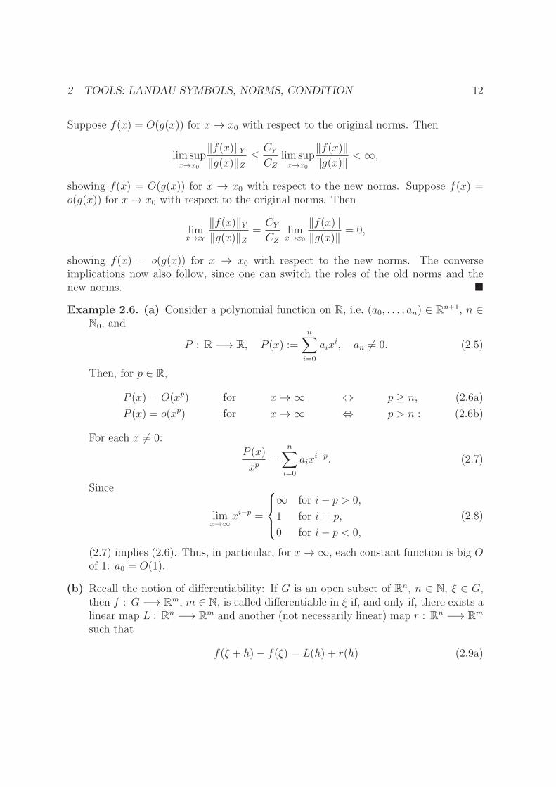
2 TOOLS: LANDAU SYMBOLS, NORMS, CONDITION 12
Suppose f(x) = O(g(x)) for x→ x0 with respect to the original norms. Then
lim supx→x0
‖f(x)‖Y‖g(x)‖Z
≤ CY
CZ
lim supx→x0
‖f(x)‖‖g(x)‖ <∞,
showing f(x) = O(g(x)) for x → x0 with respect to the new norms. Suppose f(x) =o(g(x)) for x→ x0 with respect to the original norms. Then
limx→x0
‖f(x)‖Y‖g(x)‖Z
=CY
CZ
limx→x0
‖f(x)‖‖g(x)‖ = 0,
showing f(x) = o(g(x)) for x → x0 with respect to the new norms. The converseimplications now also follow, since one can switch the roles of the old norms and thenew norms. �
Example 2.6. (a) Consider a polynomial function on R, i.e. (a0, . . . , an) ∈ Rn+1, n ∈N0, and
P : R −→ R, P (x) :=n∑
i=0
aixi, an 6= 0. (2.5)
Then, for p ∈ R,
P (x) = O(xp) for x→∞ ⇔ p ≥ n, (2.6a)
P (x) = o(xp) for x→∞ ⇔ p > n : (2.6b)
For each x 6= 0:P (x)
xp=
n∑
i=0
aixi−p. (2.7)
Since
limx→∞
xi−p =
∞ for i− p > 0,
1 for i = p,
0 for i− p < 0,
(2.8)
(2.7) implies (2.6). Thus, in particular, for x→∞, each constant function is big Oof 1: a0 = O(1).
(b) Recall the notion of differentiability: If G is an open subset of Rn, n ∈ N, ξ ∈ G,then f : G −→ Rm, m ∈ N, is called differentiable in ξ if, and only if, there exists alinear map L : Rn −→ Rm and another (not necessarily linear) map r : Rn −→ Rm
such that
f(ξ + h)− f(ξ) = L(h) + r(h) (2.9a)

2 TOOLS: LANDAU SYMBOLS, NORMS, CONDITION 13
for each h ∈ Rn with sufficiently small ‖h‖2, and
limh→0
r(h)
‖h‖2= 0. (2.9b)
Now, using the Landau symbol o, (2.9b) can be equivalently expressed as
r(h) = o(h) for h→ 0. (2.9c)
—
In the literature, one also finds statements of the form f(x) = h(x)+ o(g(x)), which arenot covered by Def. 2.2 since, according to Def. 2.2, o(g(x)) does not denote an elementof a set, i.e. adding o(g(x)) to (or otherwise combining it with) an element of a set doesnot immediately make any sense. To give a meaning to such expressions is the purposeof the following definition:
Definition 2.7. As in Def. 2.2, let (X, d) be a metric space, let (Y, ‖ · ‖), (Z, ‖ · ‖)be normed vector spaces over K, let D ⊆ X and consider functions f : D −→ Y ,g : D −→ Z, where g(x) 6= 0 for each x ∈ D. Moreover, let x0 ∈ X be a cluster point ofD. Now let (V, ‖ · ‖) be another normed vector space and let S ⊆ V be a subset1 and,for each x ∈ D, let Fx : S −→ Y be invertible on f(D) ⊆ Y . Define
f(x) = Fx
(O(g(x))
)for x→ x0 :⇔ F−1
x (f(x)) = O(g(x)) for x→ x0,
f(x) = Fx
(o(g(x))
)for x→ x0 :⇔ F−1
x (f(x)) = o(g(x)) for x→ x0.
Example 2.8. (a) In the situation of Ex. 2.6(b), we can now state that f is differen-tiable in ξ if, and only if, there exists a linear map L : Rn −→ Rm such that
f(ξ + h)− f(ξ) = L(h) + o(h) for h→ 0 : (2.10)
Indeed, for each h ∈ Rn, the map
Fh : Rm −→ Rm, Fh(s) := L(h) + s,
is invertible and, by Def. 2.7,
f(ξ + h)− f(ξ) = L(h) + o(h) = Fh(o(h)) for h→ 0
is equivalent to
r(h) := f(ξ + h)− f(ξ)− L(h) = F−1h
(f(ξ + h)− f(ξ)
)= o(h),
which is (2.9c).
1Even though, when using this kind of notation, one typically thinks of Fx as operating on g(x), asO(x) and o(x) are merely notations and not actual mathematical objects, it is not even necessary forS to contain g(D).

2 TOOLS: LANDAU SYMBOLS, NORMS, CONDITION 14
(b) Using the notation of Def. 2.7, we claim
sin x = x ln(O(1)) for x→ 0 : (2.11)
Indeed, for each x ∈ R \ {0}, the map
Fx : R+ −→ R, Fx(s) := x ln s,
is invertible with F−1x : R −→ R+, F−1
x (y) := exp( yx) and, by Def. 2.7, (2.11) is
equivalent to
F−1x (sin x) = e
sin xx = O(1),
which holds, due to limx→0 exp(sinxx) = e1 = e.
(c) Let I ⊆ R be an open interval and a, x ∈ I, x 6= a. If m ∈ N0 and f ∈ Cm+1(I),then
f(x) = Tm(x, a) +Rm(x, a), (2.12a)
where
Tm(x, a) :=m∑
k=0
f (k)(a)
k!(x− a)k (2.12b)
is the mth Taylor polynomial and
Rm(x, a) :=f (m+1)(θ)
(m+ 1)!(x− a)m+1 with some suitable θ ∈]x, a[ (2.12c)
is the Lagrange form of the remainder term. Since the continuous function f (m+1)
is bounded on each compact interval [a, y], y ∈ I, (2.12) imply
f(x) = Tm(x, a) +O((x− a)m+1
)
for x→ x0 for each x0 ∈ I.
Proposition 2.9. As in Def. 2.2, let (X, d) be a metric space, let (Y, ‖ · ‖), (Z, ‖ · ‖)be normed vector spaces over K, let D ⊆ X and consider functions f : D −→ Y ,g : D −→ Z, where g(x) 6= 0 for each x ∈ D. Moreover, let x0 ∈ X be a cluster pointof D.
(a) Suppose ‖f‖ ≤ ‖g‖ in some neighborhood of x0, i.e. there exists ǫ > 0 such that
‖f(x)‖ ≤ ‖g(x)‖ for each x ∈ D \ {x0} with d(x, x0) < ǫ.
Then f(x) = O(g(x)) for x→ x0.

2 TOOLS: LANDAU SYMBOLS, NORMS, CONDITION 15
(b) f(x) = O(f(x)) for x→ x0, but not f(x) = o(f(x)) for x→ x0 (assuming f 6= 0).
(c) f(x) = o(g(x)) for x→ x0 implies f(x) = O(g(x)) for x→ x0.
Proof. Exercise. �
Proposition 2.10. As in Def. 2.2, let (X, d) be a metric space, let (Y, ‖ · ‖), (Z, ‖ · ‖)be normed vector spaces over K, let D ⊆ X and consider functions f : D −→ Y ,g : D −→ Z, where g(x) 6= 0 for each x ∈ D. Moreover, let x0 ∈ X be a cluster pointof D. In addition, for use in some of the following assertions, we introduce functionsf1 : D −→ Y1, f2 : D −→ Y2, g1 : D −→ Z1, g2 : D −→ Z2, where (Y1, ‖ · ‖), (Y2, ‖ · ‖),(Z1, ‖ · ‖), (Z2, ‖ · ‖) are normed vector spaces over K. Assume g1(x) 6= 0 and g2(x) 6= 0for each x ∈ D.
(a) If f(x) = O(g(x)) (resp. f(x) = o(g(x))) for x→ x0, and if ‖f1‖ ≤ ‖f‖ and ‖g‖ ≤‖g1‖ in some neighborhood of x0, then f1(x) = O(g1(x)) (resp. f1(x) = o(g1(x)))for x→ x0.
(b) If α ∈ K \ {0}, then for x→ x0:
αf(x) = O(g(x)) ⇒ f(x) = O(g(x)),
αf(x) = o(g(x)) ⇒ f(x) = o(g(x)),
f(x) = O(αg(x)) ⇒ f(x) = O(g(x)),
f(x) = o(αg(x)) ⇒ f(x) = o(g(x)).
(c) For x→ x0:
f(x) = O(g1(x)) and g1(x) = O(g2(x)) implies f(x) = O(g2(x)),
f(x) = o(g1(x)) and g1(x) = o(g2(x)) implies f(x) = o(g2(x)).
(d) Assume (Y1, ‖ · ‖) = (Y2, ‖ · ‖). Then, for x→ x0:
f1(x) = O(g(x)) and f2(x) = O(g(x)) implies f1(x) + f2(x) = O(g(x)),
f1(x) = o(g(x)) and f2(x) = o(g(x)) implies f1(x) + f2(x) = o(g(x)).
(e) For x→ x0:
f1(x) = O(g1(x)) and f2(x) = O(g2(x))
implies ‖f1(x)‖ ‖f2(x)‖ = O(‖g1(x)‖ ‖g2(x)‖),f1(x) = o(g1(x)) and f2(x) = o(g2(x))
implies ‖f1(x)‖ ‖f2(x)‖ = o(‖g1(x)‖ ‖g2(x)‖).

2 TOOLS: LANDAU SYMBOLS, NORMS, CONDITION 16
(f) For x→ x0:
f(x) = O(‖g1(x)‖ ‖g2(x)‖) ⇒ ‖f(x)‖‖g1(x)‖
= O(g2(x)),
f(x) = o(‖g1(x)‖ ‖g2(x)‖) ⇒ ‖f(x)‖‖g1(x)‖
= o(g2(x)).
Proof. Exercise. �
2.2 Operator Norms and Natural Matrix Norms
When considering maps between normed vector spaces, the corresponding norms providea natural measure for error analyses. A special class of norms of importance to us areso-called operator norms defined on linear maps between normed vector spaces (cf. Def.2.12 below).
Definition 2.11. Let A : X −→ Y be a linear map between two normed vector spaces(X, ‖·‖) and (Y, ‖·‖) over K. Then A is called bounded if, and only if, A maps boundedsets to bounded sets, i.e. if, and only if, A(B) is a bounded subset of Y for each boundedB ⊆ X. The vector space of all bounded linear maps between X and Y is denoted byL(X, Y ).
Definition 2.12. Let A : X −→ Y be a linear map between two normed vector spaces(X, ‖ · ‖) and (Y, ‖ · ‖) over K. The number
‖A‖ := sup
{‖Ax‖‖x‖ : x ∈ X, x 6= 0
}
=sup{‖Ax‖ : x ∈ X, ‖x‖ = 1
}∈ [0,∞] (2.13)
is called the operator norm of A induced by the norms on X and Y , respectively (strictlyspeaking, the term operator norm is only justified if the value is finite, but it is oftenconvenient to use the term in the generalized way defined here).
In the special case, where X = Kn, Y = Km, and A is given via a real m × n matrix,the operator norm is also called a natural matrix norm or an induced matrix norm.
Remark 2.13. According to Th. B.1 of the Appendix, for a linear map A : X −→Y between two normed vector spaces X and Y over K, the following statements areequivalent:
(a) A is bounded.

2 TOOLS: LANDAU SYMBOLS, NORMS, CONDITION 17
(b) ‖A‖ <∞.
(c) A is Lipschitz continuous.
(d) A is continuous.
(e) There is x0 ∈ X such that A is continuous at x0.
For linear maps between finite-dimensional spaces, the above equivalent properties al-ways hold: Each linear map A : Kn −→ Km, (n,m) ∈ N2, is continuous (cf. [Phi16b,Ex. 2.16]). In particular, each linear map A : Kn −→ Km, has all the above equivalentproperties.
Remark 2.14. According to Th. B.2 of the Appendix, for two normed vector spaces Xand Y over K, the operator norm does, indeed, constitute a norm on the vector space ofbounded linear maps L(X, Y ), and, moreover, if A ∈ L(X, Y ), then ‖A‖ is the smallestLipschitz constant for A.
Lemma 2.15. If Id : X −→ X, Id(x) := x, is the identity map on a normed vectorspace X over K, then ‖ Id ‖ = 1 (in particular, the operator norm of a unit matrix isalways 1). Caveat: In principle, one can consider two different norms on X simultane-ously, and then the operator norm of the identity can differ from 1.
Proof. If ‖x‖ = 1, then ‖ Id(x)‖ = ‖x‖ = 1. �
Lemma 2.16. Let X, Y, Z be normed vector spaces over K and consider linear mapsA ∈ L(X, Y ), B ∈ L(Y, Z). Then
‖BA‖ ≤ ‖B‖ ‖A‖. (2.14)
Proof. Let x ∈ X with ‖x‖ = 1. If Ax = 0, then ‖B(A(x))‖ = 0 ≤ ‖B‖ ‖A‖. If Ax 6= 0,then one estimates
∥∥B(Ax)∥∥ = ‖Ax‖
∥∥∥∥B(
Ax
‖Ax‖
)∥∥∥∥ ≤ ‖A‖ ‖B‖,
thereby establishing the case. �
Notation 2.17. For each m,n ∈ N, let M(m,n,K) ∼= Kmn denote the vector spaceover K of m × n matrices (akl) := (akl)(k,l)∈{1,...,m}×{1,...,n} over K. Moreover, we defineM(n,K) :=M(n, n,K).
Example 2.18. Let m,n ∈ N and let A : Kn −→ Km be the K-linear map given by(akl) ∈M(m,n,K) (with respect to the standard bases of Kn and Km, respectively).

2 TOOLS: LANDAU SYMBOLS, NORMS, CONDITION 18
(a) The norm defined by
‖A‖∞ := max
{n∑
l=1
|akl| : k ∈ {1, . . . ,m}}
is called the row sum norm of A. It is an exercise to show that ‖A‖∞ is the operatornorm induced if Kn and Km are endowed with the ∞-norm.
(b) The norm defined by
‖A‖1 := max
{m∑
k=1
|akl| : l ∈ {1, . . . , n}}
is called the column sum norm of A. It is an exercise to show that ‖A‖1 is theoperator norm induced if Kn and Km are endowed with the 1-norm.
(c) The operator norm on A induced if Kn and Km are endowed with the 2-norm(i.e. the Euclidean norm) is called the spectral norm of A and is denoted ‖A‖2.Unfortunately, there is no formula as simple as the ones in (a) and (b) for thecomputation of ‖A‖2. We will see in Th. 2.24 below that the value of ‖A‖2 isrelated to the eigenvalues of A∗A.
Caveat 2.19. Let m,n ∈ N and p ∈ [1,∞]. Let A : Kn −→ Km be the K-linearmap given by (akl) ∈ M(m,n,K) (with respect to the standard bases of Kn and Km,respectively). It is common to denote the operator norm on A ∈ L(Kn,Km) induced bythe p-norms on Kn and Km, respectively, by ‖A‖p (as we did in Ex. 2.18 for p =∞, 1, 2).However, for n,m > 1, the operator norm ‖·‖p is not(!) the p-norm onKmn ∼= L(Kn,Km)(the 2-norm on Kmn is known as the Frobenius norm or the Hilbert-Schmidt norm onKmn). As it turns out, for n > 1, the p-norm on Kn2
is not an operator norm inducedby any norm on Kn at all: Let
‖A‖p,nop :=
{(∑n
k=1
∑nl=1 |akl|p)1/p for p <∞,
max{|akl| : k, l ∈ {1, . . . , n}} for p =∞,
denote the p-norm on Kn2. If p ∈ [1,∞[, then
‖ Id ‖p,nop = p√n 6= 1 for n > 1,
showing that ‖ · ‖p,nop does not satisfy Lem. 2.15. If akl := 1 for each k, l ∈ {1, . . . , n},then
n = ‖AA‖∞,nop > ‖A‖∞,nop · ‖A‖∞,nop = 1 · 1 = 1 for n > 1,
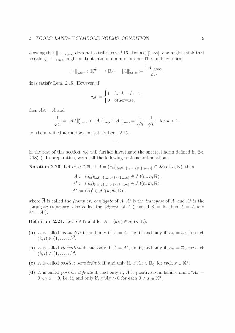
2 TOOLS: LANDAU SYMBOLS, NORMS, CONDITION 19
showing that ‖ · ‖∞,nop does not satisfy Lem. 2.16. For p ∈ [1,∞[, one might think thatrescaling ‖ · ‖p,nop might make it into an operator norm: The modified norm
‖ · ‖′p,nop : Kn2 −→ R+0 , ‖A‖′p,nop :=
‖A‖p,nopp√n
,
does satisfy Lem. 2.15. However, if
akl :=
{1 for k = l = 1,
0 otherwise,
then AA = A and
1p√n= ‖AA‖′p,nop > ‖A‖′p,nop · ‖A‖′p,nop =
1p√n· 1
p√n
for n > 1,
i.e. the modified norm does not satisfy Lem. 2.16.
—
In the rest of this section, we will further investigate the spectral norm defined in Ex.2.18(c). In preparation, we recall the following notions and notation:
Notation 2.20. Let m,n ∈ N. If A = (akl)(k,l)∈{1,...,m}×{1,...,n} ∈M(m,n,K), then
A := (akl)(k,l)∈{1,...,m}×{1,...,n} ∈M(m,n,K),
At := (akl)(l,k)∈{1,...,n}×{1,...,m} ∈M(n,m,K),
A∗ := (A)t ∈M(n,m,K),
where A is called the (complex) conjugate of A, At is the transpose of A, and A∗ is theconjugate transpose, also called the adjoint, of A (thus, if K = R, then A = A andA∗ = At).
Definition 2.21. Let n ∈ N and let A = (akl) ∈M(n,K).
(a) A is called symmetric if, and only if, A = At, i.e. if, and only if, akl = alk for each(k, l) ∈ {1, . . . , n}2.
(b) A is called Hermitian if, and only if, A = A∗, i.e. if, and only if, akl = alk for each(k, l) ∈ {1, . . . , n}2.
(c) A is called positive semidefinite if, and only if, x∗Ax ∈ R+0 for each x ∈ Kn.
(d) A is called positive definite if, and only if, A is positive semidefinite and x∗Ax =0 ⇔ x = 0, i.e. if, and only if, x∗Ax > 0 for each 0 6= x ∈ Kn.
2 TOOLS: LANDAU SYMBOLS, NORMS, CONDITION 20
Lemma 2.22. Let m,n ∈ N and A ∈ M(m,n,K). Then both A∗A ∈ M(n,K) andAA∗ ∈M(m,K) are Hermitian and positive semidefinite.
Proof. Since (A∗)∗ = A, it suffices to consider A∗A. That A∗A is Hermitian due to
(A∗A)∗ = A∗(A∗)∗ = A∗A.
Moreover, if x ∈ Kn, then x∗A∗Ax = (Ax)∗(Ax) = ‖Ax‖22 ∈ R+0 , showing A
∗A to bepositive semidefinite. �
Definition 2.23. We define, for each n ∈ N and each A ∈M(n,C),
r(A) := max{|λ| : λ ∈ C and λ is eigenvalue of A
}. (2.15)
The number r(A) is called the spectral radius of A.
Theorem 2.24. Let m,n ∈ N. If A ∈ M(m,n,K), then its spectral norm ‖A‖2 (cf.Ex. 2.18(c)) satisfies
‖A‖2 =√r(A∗A). (2.16a)
If m = n and A is Hermitian (i.e. A∗ = A), then ‖A‖2 is also given by the followingsimpler formula:
‖A‖2 = r(A). (2.16b)
Proof. According to Lem. 2.22, A∗A is a Hermitian and positive semidefinite n × nmatrix. Then there exist (cf. [Phi19b, Th. 10.41, Th. 11.3(a)]) real nonnegative (notnecessarily distinct) eigenvalues λ1, . . . , λn ≥ 0 and a corresponding ordered orthonormalbasis (v1, . . . , vn) of K
n, consisting of eigenvectors satisfying, in particular,
A∗Avk = λkvk for each k ∈ {1, . . . , n}.
As (v1, . . . , vn) is a basis of Kn, for each x ∈ Kn, there are numbers x1, . . . , xn ∈ K suchthat x =
∑nk=1 xkvk. Thus, one computes
‖Ax‖22 = (Ax) · (Ax) = x∗A∗Ax =
(n∑
k=1
xkvk
)∗ ( n∑
k=1
xkλkvk
)
=n∑
k=1
λk|xk|2 ≤ r(A∗A)n∑
k=1
|xk|2 = r(A∗A)‖x‖22, (2.17)
proving ‖A‖2 ≤√r(A∗A). To verify the remaining inequality, let λj := r(A∗A) be the
largest of the nonnegative λk, and let v := vj be the corresponding eigenvector from theorthonormal basis. Then ‖v‖2 = 1 and choosing x = v = vj (i.e. xk = δjk) in (2.17)

2 TOOLS: LANDAU SYMBOLS, NORMS, CONDITION 21
yields ‖Av‖22 = r(A∗A), thereby proving ‖A‖2 ≥√r(A∗A) and completing the proof of
(2.16a). It remains to consider the case where A = A∗. Then A∗A = A2 and, since
Av = λv ⇒ A2v = λ2v ⇒ r(A2) = r(A)2,
we have‖A‖2 =
√r(A∗A) =
√r(A2) = r(A),
thereby establishing the case. �
Caveat 2.25. In general, it is not admissible to use the simpler formula (2.16b) for
non-Hermitian n× n matrices: For example, for A :=
(0 10 1
), one has
A∗A =
(0 01 1
)(0 10 1
)=
(0 00 2
),
such that 1 = r(A) 6=√2 =
√r(A∗A) = ‖A‖2.
Lemma 2.26. Let n ∈ N. Then
‖y‖2 = max{|v · y| : v ∈ Kn and ‖v‖2 = 1
}for each y ∈ Kn. (2.18)
Proof. Let v ∈ Kn such that ‖v‖2 = 1. One estimates, using the Cauchy-Schwarzinequality [Phi16b, (1.41)],
|v · y| ≤ ‖v‖2‖y‖2 = ‖y‖2. (2.19a)
Note that (2.18) is trivially true for y = 0. If y 6= 0, then letting w := y/‖y‖2 yields‖w‖2 = 1 and
|w · y| =∣∣y · y/‖y‖2
∣∣ = ‖y‖2. (2.19b)
Together, (2.19a) and (2.19b) establish (2.18). �
Proposition 2.27. Let m,n ∈ N. If A ∈ M(m,n,K), then ‖A‖2 = ‖A∗‖2 and, inparticular, r(A∗A) = r(AA∗). This allows one to use the simpler (smaller) matrix ofA∗A and AA∗ to compute ‖A‖2 (see Ex. 2.29 below).
Proof. We know from Linear Algebra (cf. [Phi19b, Th. 10.22(a)] and [Phi19b, Th.10.24(a)]) that
∀x∈Kn
∀v∈Km
v · Ax = (A∗v) · x.
2 TOOLS: LANDAU SYMBOLS, NORMS, CONDITION 22
Thus, one calculates
‖A‖2 = max{‖Ax‖2 : x ∈ Kn and ‖x‖2 = 1
}
(2.18)= max
{|v · Ax| : v ∈ Km, x ∈ Kn, and ‖v‖2 = ‖x‖2 = 1
}
= max{|(A∗v) · x| : v ∈ Km, x ∈ Kn, and ‖v‖2 = ‖x‖2 = 1
}
(2.18)= max
{‖A∗v‖2 : v ∈ Km and ‖v‖2 = 1
}
= ‖A∗‖2,proving the proposition. �
Remark 2.28. One can actually show more than we did in Prop. 2.27: The eigenvalues(including multiplicities) of A∗A and AA∗ are always identical, except that the larger ofthe two matrices (if any) can have additional eigenvalues of value 0 – the square roots ofthe nonzero (i.e. positive) eigenvalues of A∗A and AA∗ are the so-called singular valuesof A and A∗ (see, e.g., [HB09, Def. and Th. 12.1]).
Example 2.29. Consider A :=
(1 0 1 00 1 1 0
)∈M(2, 4,K). One obtains
AA∗ =
(2 11 2
), A∗A =
1 0 1 00 1 1 01 1 2 00 0 0 0
.
So one would tend to compute the eigenvalues using AA∗. One finds λ1 = 1 and λ2 = 3.Thus, r(AA∗) = 3 and ‖A‖2 =
√3.
2.3 Condition of a Problem
We are now in a position to apply our acquired knowledge of operator norms to erroranalysis. The general setting is the following: The input is given in some normed vectorspace X (e.g. Kn) and the output is likewise a vector lying in some normed vector spaceY (e.g. Km). The solution operator, i.e. the map f between input and output, is somefunction f defined on an open subset of X. The goal in this section is to study thebehavior of the output given small changes (errors) of the input.
Definition 2.30. Let (X, ‖ · ‖) and (Y, ‖ · ‖) be normed vector spaces over K, U ⊆ Xopen, and f : U −→ Y . Fix x ∈ U \ {0} such that f(x) 6= 0 and δ > 0 such thatBδ(x) = {x ∈ X : ‖x− x‖ < δ} ⊆ U . We call (the problem represented by the solutionoperator) f well-conditioned in Bδ(x) if, and only if, there exists K ≥ 0 such that
‖f(x)− f(x)‖‖f(x)‖ ≤ K
‖x− x‖‖x‖ for every x ∈ Bδ(x). (2.20)

2 TOOLS: LANDAU SYMBOLS, NORMS, CONDITION 23
If f is well-conditioned in Bδ(x), then we define K(δ) := K(f, x, δ) to be the smallestnumber K ∈ R+
0 such that (2.20) is valid. If there exists δ > 0 such that f is well-conditioned in Bδ(x), then f is called well-conditioned at x.
Definition and Remark 2.31. We remain in the situation of Def. 2.30 and notice that0 < α ≤ β ≤ δ implies Bα(x) ⊆ Bβ(x) ⊆ Bδ(x), and, thus 0 ≤ K(α) ≤ K(β) ≤ K(δ).In consequence, the following definition makes sense if f is well-conditioned at x:
krel := krel(f, x) := limα→0
K(α). (2.21)
The number krel ∈ R+0 is called the relative condition of (the problem represented by the
solution operator) f at x. The number krel provides a measure for how much a relativeerror in x might get inflated by the application of f , i.e. the smaller krel, the more well-behaved is the problem in the vicinity of x. What value for krel is still acceptable interms of numerical stability depends on the situation: While krel ≈ 1 generally indicatesstability, even krel ≈ 100 might be acceptable in some situations.
Remark 2.32. Let us compare the newly introduced notion of Def. and Rem. 2.31 off being well-conditioned with some other regularity notions for f . For example, if f isL-Lipschitz in Bδ(x), x ∈ X, δ > 0, then
∀x∈Bδ(x)
‖f(x)− f(x)‖ ≤ L ‖x− x‖,
i.e. f is well-conditioned in Bδ(x) and (2.20) holds with K := L ‖x‖‖f(x)‖ . The converse is not
true: There are examples, where f is well-conditioned in some Bδ(x) without being Lip-schitz continuous on Bδ(x) (exercise). On the other hand, (2.20) does imply continuityin x, and, once again, the converse is not true (another exercise). In particular, a prob-lem can be well-posed in the sense of Def. 1.5 without being well-conditioned. On theother hand, if f is everywhere well-conditioned, then it is everywhere continuous, and,thus, well-posed. In that sense well-conditionedness is stronger than well-posedness.However, one should also note that we defined well-conditionedness as a local property,whereas well-posedness was defined as a global property.
—
As an example, we consider the problem of solving the linear system Ax = b with aninvertible n×n matrix A ∈M(n,K). Before studying the problem systematically usingthe notion of well-conditionedness, let us look at a particular example that illustrates atypical instability that can occur:
Example 2.33. Consider the linear system
Ax = b
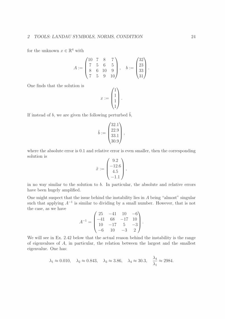
2 TOOLS: LANDAU SYMBOLS, NORMS, CONDITION 24
for the unknown x ∈ R4 with
A :=
10 7 8 77 5 6 58 6 10 97 5 9 10
, b :=
32233331
.
One finds that the solution is
x :=
1111
.
If instead of b, we are given the following perturbed b,
b :=
32.122.933.130.9
,
where the absolute error is 0.1 and relative error is even smaller, then the correspondingsolution is
x :=
9.2−12.64.5−1.1
,
in no way similar to the solution to b. In particular, the absolute and relative errorshave been hugely amplified.
One might suspect that the issue behind the instability lies in A being “almost” singularsuch that applying A−1 is similar to dividing by a small number. However, that is notthe case, as we have
A−1 =
25 −41 10 −6−41 68 −17 1010 −17 5 −3−6 10 −3 2
.
We will see in Ex. 2.42 below that the actual reason behind the instability is the rangeof eigenvalues of A, in particular, the relation between the largest and the smallesteigenvalue. One has:
λ1 ≈ 0.010, λ2 ≈ 0.843, λ3 ≈ 3.86, λ4 ≈ 30.3,λ4λ1≈ 2984.

2 TOOLS: LANDAU SYMBOLS, NORMS, CONDITION 25
Proposition 2.34. Let m,n ∈ N and consider the normed vector spaces (Kn, ‖ · ‖) and(Km, ‖ · ‖). Let A : Kn −→ Km be K-linear. Moreover, let x ∈ Kn be such that x 6= 0and Ax 6= 0. Then the following statements hold true:
(a) A is well-conditioned at x and
krel(A, x) = ‖A‖‖x‖‖Ax‖ ,
where ‖A‖ denotes the corresponding operator norm of A.
(b) If n = m and A is invertible, then
krel(A, x) ≤ ‖A‖‖A−1‖,
where ‖A‖ and ‖A−1‖ denote the corresponding operator norms of A and A−1,respectively.
Proof. (a): For each x ∈ Kn, we estimate
‖Ax− Ax‖‖Ax‖ ≤ ‖A‖ ‖x− x‖‖Ax‖ = ‖A‖ ‖x‖‖Ax‖
‖x− x‖‖x‖ ,
showing krel(A, x) ≤ ‖A‖ ‖x‖‖Ax‖ . It still remains to prove the inverse inequality. To that
end, choose v ∈ Kn such that ‖v‖ = 1 and ‖Av‖ = ‖A‖ (such a vector v must exist dueto the fact that the continuous function z 7→ ‖Az‖ must attain its max on the compactunit sphere S1(0) = {z ∈ Kn : ‖z‖ = 1} – note that this argument does not work ininfinite-dimensional spaces, where S1(0) is not compact). Consider x := x+ αv. Then
‖Ax− Ax‖‖Ax‖ = α
‖Av‖‖Ax‖
‖Av‖=‖A‖, ‖v‖=1= ‖A‖ ‖x‖‖Ax‖
‖x− x‖‖x‖ .
As this equality is independent of α, for α → 0, we obtain krel(A, x) ≥ ‖A‖ ‖x‖‖Ax‖ , as
desired.
(b): If n = m and A is invertible, then (a) implies
krel(A, x) = ‖A‖‖x‖‖Ax‖ = ‖A‖‖A
−1Ax‖‖Ax‖ ≤ ‖A‖‖A
−1‖‖Ax‖‖Ax‖ = ‖A‖‖A−1‖,
thereby proving (b). �

2 TOOLS: LANDAU SYMBOLS, NORMS, CONDITION 26
Example 2.35. Let A ∈ M(n,K) be an invertible n × n matrix, n ∈ N and considerthe problem of solving the linear system Ax = b, b ∈ Kn. Then the solution operator is
A−1 : Kn −→ Kn, b 7→ A−1b.
Fixing some norm on Kn and using the induced natural matrix norm, we obtain fromProp. 2.34(b) that, for each 0 6= b ∈ Kn:
krel(A−1, b) ≤ ‖A‖‖A−1‖. (2.22)
Definition and Remark 2.36. In view of Prop. 2.34(b) and (2.22), we define thecondition number κ(A) (also just called the condition) of an invertible A ∈ M(n,K),n ∈ N, by
κ(A) := ‖A‖‖A−1‖, (2.23)
where ‖ · ‖ denotes a natural matrix norm induced by some norm on Kn. Then oneimmediately gets from (2.22) that
krel(A−1, b) ≤ κ(A) for each b ∈ Kn \ {0}. (2.24)
The condition number clearly depends on the underlying natural matrix norm. If thenatural matrix norm is the spectral norm, then one calls the condition number thespectral condition and one also writes κ2 instead of κ.
Notation 2.37. For each A ∈M(n,C), n ∈ N, let
σ(A) := {λ ∈ C : λ is eigenvalue of A},|σ(A)| := {|λ| : λ ∈ C is eigenvalue of A},
denote the set of eigenvalues of A (also known as the spectrum of A) and the set ofabsolute values of eigenvalues of A, respectively.
Lemma 2.38. For the spectral condition of an invertible matrix A ∈ M(n,K), n ∈ N,one obtains
κ2(A) =
√max σ(A∗A)
min σ(A∗A)(2.25)
(recall that all eigenvalues of A∗A are real and positive). Moreover, if A is Hermitian,then (2.25) simplifies to
κ2(A) =max |σ(A)|min |σ(A)| (2.26)
(note that min |σ(A)| > 0, as A is invertible).

2 TOOLS: LANDAU SYMBOLS, NORMS, CONDITION 27
Proof. Exercise. �
Theorem 2.39. Let A ∈M(n,K) be invertible, n ∈ N. Assume that x, b,∆x,∆b ∈ Kn
satisfyAx = b, A(x+∆x) = b+∆b, (2.27)
i.e. ∆b can be seen as a perturbation of the input and ∆x can be seen as the resultingperturbation of the output. One then has the following estimates for the absolute andrelative errors:
‖∆x‖ ≤ ‖A−1‖‖∆b‖, ‖∆x‖‖x‖ ≤ κ(A)
‖∆b‖‖b‖ , (2.28)
where x, b 6= 0 is assumed for the second estimate (as before, it does not matter whichnorm on Kn one uses, as long as one uses the induced operator norm for the matrix).
Proof. Since A is linear, (2.27) implies A(∆x) = ∆b, i.e. ∆x = A−1(∆b), which alreadyyields the first estimate in (2.28). For x, b 6= 0, the first estimate together with Ax = beasily implies the second:
‖∆x‖‖x‖ ≤ ‖A
−1‖ ‖∆b‖‖b‖‖Ax‖‖x‖ ,
thereby establishing the case. �
Example 2.40. Suppose we want to find out how much we can perturb b in the problem
Ax = b, A :=
(−1 2−3 4
), b :=
(5−2
),
if the resulting relative error er in x is to be less than 10−2 with respect to the∞-norm.From (2.28), we know
er ≤ κ(A)‖∆b‖∞‖b‖∞
= κ(A)‖∆b‖∞
5.
Moreover, since A−1 = 12
(4 −23 −1
), from (2.23) and Ex. 2.18(a), we obtain
κ(A) = ‖A‖∞‖A−1‖∞ = 7 · 72=
49
2.
Thus, if the perturbation ∆b satisfies ‖∆b‖∞ < 1490≈ 0.0020, then er <
492·5 · 1
490= 10−2.
Remark 2.41. Note that (2.28) is a much stronger and more useful statement thanthe krel(A
−1, b) ≤ κ(A) of (2.22). The relative condition only provides a bound in thelimit of smaller and smaller neighborhoods of b and without providing any information

2 TOOLS: LANDAU SYMBOLS, NORMS, CONDITION 28
on how small the neighborhood actually has to be (one can estimate the amplificationof the error in x provided that the error in b is very small). On the other hand, (2.28)provides an effective control of the absolute and relative errors without any restrictionswith regard to the size of the error in b (it holds for each ∆b).
—
Example 2.42. We come back to the instability observed in Ex. 2.33 and investigateits actual cause. Suppose A ∈ M(n,C) is an arbitrary Hermitian invertible matrix,λmin, λmax ∈ σ(A) such that |λmin| = min |σ(A)|, |λmax| = max |σ(A)|. Let vmin and vmax
be eigenvectors for λmin and λmax, respectively, satisfying ‖vmin‖ = ‖vmax‖ = 1. Themost unstable behavior of Ax = b occurs if b = vmax and b is perturbed in the directionof vmin, i.e. b := b + ǫ vmin, ǫ > 0. The solution to Ax = b is x = λ−1
maxvmax, whereas thesolution to Ax = b is
x = A−1(vmax + ǫ vmin) = λ−1maxvmax + ǫλ−1
minvmin.
Thus, the resulting relative error in the solution is
‖x− x‖‖x‖ = ǫ
|λmax||λmin|
,
while the relative error in the input was merely
‖b− b‖‖b‖ = ǫ.
This shows that, in the worst case, the relative error in b can be amplified by a factorof κ2(A) = |λmax|/|λmin|, and that is exactly what had occurred in Ex. 2.33.
—
Next, we study a generalization of the problem from (2.27). Now, in addition to aperturbation of the right-hand side b, we also allow a perturbation of the matrix A bya matrix ∆A:
Ax = b, (A+∆A)(x+∆x) = b+∆b. (2.29)
We would now like to control ∆x in terms of ∆b and ∆A.
Remark 2.43. Let n ∈ N. The set GLn(K) of invertible n× n matrices over K is openinM(n,K) ∼= Kn2
(where all norms are equivalent) – this follows, for example, from thedeterminant being a continuous map (even a polynomial, cf. [Phi19b, Rem. 4.33]) fromKn2
into K, which implies that GLn(K) = det−1(K \ {0}) must be open. Thus, if A in(2.29) is invertible and ‖∆A‖ is sufficiently small, then A+∆A must also be invertible.

2 TOOLS: LANDAU SYMBOLS, NORMS, CONDITION 29
Lemma 2.44. Let n ∈ N, consider some norm on Kn, and the induced natural matrixnorm onM(n,K). If B ∈M(n,K) is such that ‖B‖ < 1, then Id+B is invertible and
‖(Id+B)−1‖ ≤ 1
1− ‖B‖ . (2.30)
Proof. For each x ∈ Kn:
‖(Id+B)x‖ ≥ ‖x‖ − ‖Bx‖ ≥ ‖x‖ − ‖B‖ ‖x‖ = (1− ‖B‖) ‖x‖, (2.31)
showing that x 6= 0 implies (Id+B)x 6= 0, i.e. Id+B is invertible. Fixing y ∈ Kn andapplying (2.31) with x := (Id+B)−1y yields
‖(Id+B)−1y‖ ≤ 1
1− ‖B‖ ‖y‖,
thereby proving (2.30) and concluding the proof of the lemma. �
Lemma 2.45. Let n ∈ N, consider some norm on Kn and the induced natural matrixnorm on M(n,K). If A,∆A ∈ M(n,K), A is invertible, and ‖∆A‖ < ‖A−1‖−1, thenA+∆A is invertible and
‖(A+∆A)−1‖ ≤ 1
‖A−1‖−1 − ‖∆A‖ . (2.32)
Moreover,
‖∆A‖ ≤ 1
2‖A−1‖ ⇒ ‖(A+∆A)−1 − A−1‖ ≤ C‖∆A‖, (2.33)
where the constant can be chosen as C := 2‖A−1‖2.
Proof. We can write A + ∆A = A(Id+A−1∆A). As ‖A−1∆A‖ ≤ ‖A−1‖ ‖∆A‖ < 1,Lem. 2.44 yields that Id+A−1∆A is invertible. Since A is also invertible, so is A+∆A.Moreover,
‖(A+∆A)−1‖ =∥∥(Id+A−1∆A)−1A−1
∥∥ (2.30)
≤ ‖A−1‖1− ‖A−1∆A‖ ≤
‖A−1‖1− ‖A−1‖ ‖∆A‖ ,
(2.34)proving (2.32). The identity
(A+∆A)−1 − A−1 = −(A+∆A)−1(∆A)A−1 (2.35)
holds, as it is equivalent to
Id−(A+∆A)A−1 = −(∆A)A−1

2 TOOLS: LANDAU SYMBOLS, NORMS, CONDITION 30
andA− A−∆A = −∆A.
For ‖∆A‖ ≤ 12‖A−1‖ , (2.35) yields
‖(A+∆A)−1 − A−1‖ ≤ ‖(A+∆A)−1‖ ‖∆A‖ ‖A−1‖(2.34)
≤ ‖A−1‖ ‖∆A‖ ‖A−1‖1− ‖A−1‖ ‖∆A‖
≤ 2 ‖A−1‖2 ‖∆A‖,
proving (2.33). �
Theorem 2.46. As in Lem. 2.45, let n ∈ N, consider some norm on Kn with theinduced natural matrix norm onM(n,K) and let A,∆A ∈M(n,K) such A is invertibleand ‖∆A‖ < ‖A−1‖−1. Moreover, assume b, x,∆b,∆x ∈ Kn satisfy
Ax = b, (A+∆A)(x+∆x) = b+∆b. (2.36)
Then, for b, x 6= 0, one has the following bound for the relative error:
‖∆x‖‖x‖ ≤
κ(A)
1− ‖A−1‖ ‖∆A‖
(‖∆A‖‖A‖ +
‖∆b‖‖b‖
). (2.37)
Proof. The equations (2.36) imply
(A+∆A)(∆x) = ∆b− (∆A)x. (2.38)
In consequence, from (2.32) and ‖b‖ ≤ ‖A‖ ‖x‖, one obtains
‖∆x‖‖x‖
(2.38)=
∥∥∥(A+∆A)−1(∆b− (∆A)x
)∥∥∥‖x‖
(2.32)
≤ 1
‖A−1‖−1 − ‖∆A‖
(‖∆A‖+ ‖∆b‖‖A‖‖b‖
)
=κ(A)
1− ‖A−1‖ ‖∆A‖
(‖∆A‖‖A‖ +
‖∆b‖‖b‖
),
thereby establishing the case. �
For nonlinear problems, the following result can be useful:
Theorem 2.47. Let m,n ∈ N, let U ⊆ Rn be open, and assume that f : U −→ Rm
is continuously differentiable: f ∈ C1(U,Rm). If 0 6= x ∈ U and f(x) 6= 0, then f iswell-conditioned at x and
krel = krel(f, x) = ‖Df(x)‖‖x‖‖f(x)‖ , (2.39)

2 TOOLS: LANDAU SYMBOLS, NORMS, CONDITION 31
where Df(x) : Rn −→ Rm is the (total) derivative of f in x (which is a linear maprepresented by the Jacobian Jf (x)). In (2.39), any norm on Rn and Rm will work aslong as ‖Df(x)‖ is the corresponding induced operator norm. While the present result isonly formulated and proved for R-differentiable functions, see Rem. 2.48 and Ex. 2.49(c)below to learn how it can also be applied to C-differentiable functions.
Proof. Choose δ > 0 sufficiently small such that Bδ(x) ⊆ U . Since f ∈ C1(U,Rm), wecan apply Taylor’s theorem. Recall that its lowest order version with the remainderterm in integral form states that, for each h ∈ Bδ(0) (which implies x + h ∈ Bδ(x)),the following holds (cf. [Phi16b, Th. 4.44], which can be applied to the componentsf1, . . . , fm of f):
f(x+ h) = f(x) +
∫ 1
0
Df(x+ th
)(h) dt . (2.40)
If x ∈ Bδ(x), then we can let h := x− x, which permits to restate (2.40) in the form
f(x)− f(x) =∫ 1
0
Df((1− t)x+ tx
)(x− x) dt . (2.41)
This allows to estimate the norm as follows:
∥∥f(x)− f(x)∥∥ =
∥∥∥∥∫ 1
0
Df((1− t)x+ tx
)(x− x) dt
∥∥∥∥Th. C.5
≤∫ 1
0
∥∥∥Df((1− t)x+ tx
)(x− x)
∥∥∥ dt
≤∫ 1
0
∥∥∥Df((1− t)x+ tx
)∥∥∥ ‖x− x‖ dt
≤ sup{∥∥Df(y)
∥∥ : y ∈ Bδ(x)}‖x− x‖
= S(δ)‖x− x‖ (2.42)
with S(δ) := sup{∥∥Df(y)
∥∥ : y ∈ Bδ(x)}. This implies
∥∥f(x)− f(x)∥∥
∥∥f(x)∥∥ ≤ ‖x‖∥∥f(x)
∥∥S(δ)‖x− x‖‖x‖
and, therefore,
K(δ) ≤ ‖x‖∥∥f(x)∥∥S(δ). (2.43)
The hypothesis that f is continuously differentiable implies limy→xDf(y) = Df(x),which implies limy→x ‖Df(y)‖ = ‖Df(x)‖ (continuity of the norm, cf. [Phi16b, Ex.

2 TOOLS: LANDAU SYMBOLS, NORMS, CONDITION 32
2.6(a)]), which, in turn, implies limδ→0 S(δ) = ‖Df(x)‖. Since, also, limδ→0K(δ) = krel,(2.43) yields
krel ≤ ‖Df(x)‖‖x‖‖f(x)‖ . (2.44)
It still remains to prove the inverse inequality. To that end, choose v ∈ Rn such that‖v‖ = 1 and ∥∥Df(x)(v)
∥∥ =∥∥Df(x)
∥∥ (2.45)
(such a vector v must exist due to the fact that the continuous function y 7→ ‖Df(x)(y)‖must attain its max on the compact unit sphere S1(0) – as in the proof of Prop. 2.34(a),this argument does not extend to infinite-dimensional spaces, where S1(0) is not com-pact). For 0 < ǫ < δ consider x := x + ǫv. Then ‖x − x‖ = ǫ < δ, i.e. x ∈ Bδ(x). Inparticular, x is admissible in (2.41), which provides
f(x)− f(x) = ǫ
∫ 1
0
Df((1− t)x+ tx
)(v) dt
= ǫDf(x)(v) + ǫ
∫ 1
0
(Df((1− t)x+ tx
)−Df(x)
)(v) dt . (2.46)
Once again using ‖x − x‖ = ǫ as well as the triangle inequality in the form ‖a + b‖ ≥‖a‖ − ‖b‖, we obtain from (2.46) and (2.45):
∥∥f(x)− f(x)∥∥
∥∥f(x)∥∥
≥ ‖x‖∥∥f(x)∥∥
(∥∥Df(x)∥∥−
∫ 1
0
∥∥∥Df((1− t)x+ tx
)−Df(x)
∥∥∥ dt) ‖x− x‖‖x‖ . (2.47)
Thus,
K(ǫ) ≥ ‖x‖∥∥f(x)∥∥(∥∥Df(x)
∥∥− T (ǫ)), (2.48)
where
T (ǫ) := sup
{∫ 1
0
∥∥∥Df((1− t)x+ tx
)−Df(x)
∥∥∥ dt : x ∈ Bǫ(x)
}. (2.49)
Since Df is continuous in x, for each α > 0, there is ǫ > 0 such that ‖y−x‖ ≤ ǫ implies‖Df(y) −Df(x)‖ < α. Thus, since ‖(1 − t)x + tx − x‖ = t ‖x − x‖ ≤ ǫ for x ∈ Bǫ(x)and t ∈ [0, 1], one obtains
T (ǫ) ≤∫ 1
0
α dt = α,

2 TOOLS: LANDAU SYMBOLS, NORMS, CONDITION 33
implyinglimǫ→0
T (ǫ) = 0.
In particular, we can take limits in (2.48) to get
krel ≥‖x‖∥∥f(x)
∥∥∥∥Df(x)
∥∥. (2.50)
Finally, (2.50) together with (2.44) completes the proof of (2.39). �
Remark 2.48. While Th. 2.47 was formulated and proved for (continuously) R-differen-tiable functions, it can also be used for C-differentiable (i.e. for holomorphic) functions:Recall that C-differentiability is actually a much stronger condition than continuous R-differentiability: A function that is C-differentiable is, in particular, R-differentiable andeven C∞ (see [Phi16b, Def. 4.18] and [Phi16b, Rem. 4.19(c)]). As a concrete example,we apply Th. 2.47 to complex multiplication in Ex. 2.49(c) below. For more informationregarding the relation between norms on Cn and norms on R2n, also see [Phi16b, Sec.D].
Example 2.49. (a) Let us investigate the condition of the problem of real multiplica-tion, by considering
f : R2 −→ R, f(x, y) := xy, Df(x, y) = (y, x). (2.51)
Using the Euclidean norm ‖ · ‖2 on R2, one obtains, for each (x, y) ∈ R2 such thatxy 6= 0,
krel(x, y) := krel(f, (x, y)) = ‖Df(x, y)‖2‖(x, y)‖2|f(x, y)| =
x2 + y2
|xy| =|x||y| +
|y||x| . (2.52)
Thus, we see that the relative condition explodes if |x| ≫ |y| or |x| ≪ |y|. To showf is well-conditioned in Bδ(x, y) for each δ > 0, let (x, y) ∈ Bδ(x, y) and estimate
∣∣f(x, y)− f(x, y)∣∣ = |xy − xy| ≤ |xy − xy|+ |xy − xy| = |x||y − y|+ |y||x− x|≤ max
{‖(x, y)‖2, ‖(x, y)‖2
}∥∥(x, y)− (x, y)∥∥1
≤ C(δ + ‖(x, y)‖2
) ∥∥(x, y)− (x, y)∥∥2
with suitable C ∈ R+. Thus, f is well-conditioned in Bδ(x, y). In consequence, wesee that multiplication is numerically stable if, and only if, |x| and |y| are roughlyof the same order of magnitude.
2 TOOLS: LANDAU SYMBOLS, NORMS, CONDITION 34
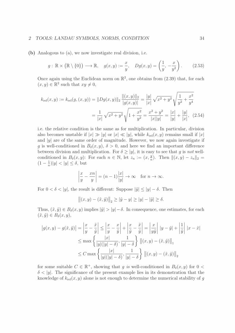
(b) Analogous to (a), we now investigate real division, i.e.
g : R×(R \ {0}
)−→ R, g(x, y) :=
x
y, Dg(x, y) =
(1
y, − x
y2
). (2.53)
Once again using the Euclidean norm on R2, one obtains from (2.39) that, for each(x, y) ∈ R2 such that xy 6= 0,
krel(x, y) := krel(g, (x, y)) = ‖Dg(x, y)‖2‖(x, y)‖2|g(x, y)| =
|y||x|√x2 + y2
√1
y2+x2
y4
=1
|x|√x2 + y2
√1 +
x2
y2=x2 + y2
|x||y| =|x||y| +
|y||x| , (2.54)
i.e. the relative condition is the same as for multiplication. In particular, divisionalso becomes unstable if |x| ≫ |y| or |x| ≪ |y|, while krel(x, y) remains small if |x|and |y| are of the same order of magnitude. However, we now again investigate ifg is well-conditioned in Bδ(x, y), δ > 0, and here we find an important differencebetween division and multiplication. For δ ≥ |y|, it is easy to see that g is not well-conditioned in Bδ(x, y): For each n ∈ N, let zn := (x, y
n). Then ‖(x, y) − zn‖2 =
(1− 1n)|y| < |y| ≤ δ, but
∣∣∣∣x
y− xn
y
∣∣∣∣ = (n− 1)|x||y| → ∞ for n→∞.
For 0 < δ < |y|, the result is different: Suppose |y| ≤ |y| − δ. Then∥∥(x, y)− (x, y)
∥∥2≥ |y − y| ≥ |y| − |y| ≥ δ.
Thus, (x, y) ∈ Bδ(x, y) implies |y| > |y|−δ. In consequence, one estimates, for each(x, y) ∈ Bδ(x, y),
∣∣g(x, y)− g(x, y)∣∣ =
∣∣∣∣x
y− x
y
∣∣∣∣ ≤∣∣∣∣x
y− x
y
∣∣∣∣+∣∣∣∣x
y− x
y
∣∣∣∣ =∣∣∣∣x
yy
∣∣∣∣ |y − y|+∣∣∣∣1
y
∣∣∣∣ |x− x|
≤ max
{ |x||y|(|y| − δ) ,
1
|y| − δ
} ∥∥(x, y)− (x, y)∥∥1
≤ Cmax
{ |x||y|(|y| − δ) ,
1
|y| − δ
} ∥∥(x, y)− (x, y)∥∥2
for some suitable C ∈ R+, showing that g is well-conditioned in Bδ(x, y) for 0 <δ < |y|. The significance of the present example lies in its demonstration that theknowledge of krel(x, y) alone is not enough to determine the numerical stability of g
2 TOOLS: LANDAU SYMBOLS, NORMS, CONDITION 35
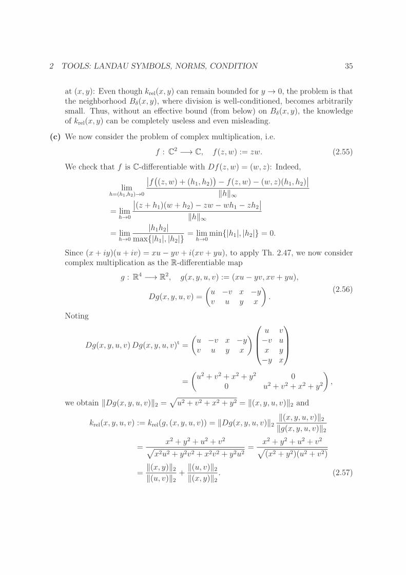
at (x, y): Even though krel(x, y) can remain bounded for y → 0, the problem is thatthe neighborhood Bδ(x, y), where division is well-conditioned, becomes arbitrarilysmall. Thus, without an effective bound (from below) on Bδ(x, y), the knowledgeof krel(x, y) can be completely useless and even misleading.
(c) We now consider the problem of complex multiplication, i.e.
f : C2 −→ C, f(z, w) := zw. (2.55)
We check that f is C-differentiable with Df(z, w) = (w, z): Indeed,
limh=(h1,h2)→0
∣∣f((z, w) + (h1, h2)
)− f(z, w)− (w, z)(h1, h2)
∣∣‖h‖∞
= limh→0
∣∣(z + h1)(w + h2)− zw − wh1 − zh2∣∣
‖h‖∞= lim
h→0
|h1h2|max{|h1|, |h2|}
= limh→0
min{|h1|, |h2|} = 0.
Since (x+ iy)(u+ iv) = xu− yv + i(xv + yu), to apply Th. 2.47, we now considercomplex multiplication as the R-differentiable map
g : R4 −→ R2, g(x, y, u, v) := (xu− yv, xv + yu),
Dg(x, y, u, v) =
(u −v x −yv u y x
).
(2.56)
Noting
Dg(x, y, u, v)Dg(x, y, u, v)t =
(u −v x −yv u y x
)
u v−v ux y−y x
=
(u2 + v2 + x2 + y2 0
0 u2 + v2 + x2 + y2
),
we obtain ‖Dg(x, y, u, v)‖2 =√u2 + v2 + x2 + y2 = ‖(x, y, u, v)‖2 and
krel(x, y, u, v) := krel(g, (x, y, u, v)) = ‖Dg(x, y, u, v)‖2‖(x, y, u, v)‖2‖g(x, y, u, v)‖2
=x2 + y2 + u2 + v2√
x2u2 + y2v2 + x2v2 + y2u2=
x2 + y2 + u2 + v2√(x2 + y2)(u2 + v2)
=‖(x, y)‖2‖(u, v)‖2
+‖(u, v)‖2‖(x, y)‖2
. (2.57)

3 INTERPOLATION 36
Thus, letting z := x+ iy and w := u+ iv, in generalization of what occurred in (a),the relative condition becomes arbitrarily large if ‖z‖2 ≫ ‖w‖2 or ‖z‖2 ≪ ‖w‖2.An estimate completely analogous to the one in (a) shows g to be well-conditionedin Bδ(x, y, u, v) = Bδ(z, w) for each δ > 0: We have, for each
(z, w) := (x, y, u, v) ∈ Bδ(x, y, u, v),
that
∥∥g(x, y, u, v)− g(x, y, u, v)∥∥2= |zw − zw| ≤ |zw − zw|+ |zw − zw|= |z||w − w|+ |w||z − z|≤ max
{‖(z, w)‖2, ‖(z, w)‖2
}∥∥(z, w)− (z, w)∥∥1
≤ C(δ + ‖(z, w)‖2
) ∥∥(z, w)− (z, w)∥∥2
= C(δ + ‖(x, y, u, v)‖2
) ∥∥(x, y, u, v)− (x, y, u, v)∥∥2
with suitable C ∈ R+.
3 Interpolation
3.1 Motivation
Given a finite number of points (x0, y0), (x1, y1), . . . , (xn, yn), so-called data points, sup-porting points, or tabular points, the goal is to find a function f such that f(xi) = yi foreach i ∈ {0, . . . , n}. Then f is called an interpolate of the data points. The data pointscan be measured values from a physical experiment or computed values (for example,it could be that yi = g(xi) and g(x) can, in principle, be computed, but it could bevery difficult and computationally expensive (g could be the solution of a differentialequation) – in that case, it can also be advantageous to interpolate the data points byan approximation f to g such that f is efficiently computable).
To have an interpolate f at hand can be desirable for many reasons, including
(a) f(x) can then be computed at an arbitrary point.
(b) If f is differentiable, then derivatives can be computed in an arbitrary point, atleast, in principle.
(c) Computation of integrals of the form∫ b
af(x) dx , if f is integrable.
(d) Determination of extreme points of f (e.g. for R-valued f).

3 INTERPOLATION 37
(e) Determination of zeros of f (e.g. for R-valued f).
While a general function f , defined on an infinite domain, is never determined by itsvalues on finitely many points, the situation can be different if it is known that f hasadditional properties, for instance, that it has to lie in a certain set of functions or thatit can at least be approximated by functions from a certain function set. For example,we will see in the next section that polynomials are determined by finitely many datapoints.
The interpolate should be chosen such that it reflects properties expected from the ex-act solution (if any). For example, polynomials are not the best choice if one expectsa periodic behavior or if the exact solution is known to have singularities. If periodicbehavior is expected, then interpolation by trigonometric functions is usually advised(cf. Sections E.2 and E.3 of the Appendix), whereas interpolation by rational functionsis often desirable if singularities are expected (cf. [FH07, Sec. 2.2]). Due to time con-straints, we will only study interpolations related to polynomials in this class, but oneshould keep in the back of one’s mind that there are other types of interpolates thatmight me more suitable, depending on the circumstances.
3.2 Polynomial Interpolation
If polynomial interpolation is to mean the problem of finding a polynomial (function)that interpolates given data points, then we will see that (cf. Th. 3.4 below), in contrastto the general interpolation problem described above, the problem is purely algebraicwith (in the absence of roundoff errors) an exact solution, not involving any approxi-mation. However, for the reasons described above, one migth then use the interpolatingpolynomial as an approximation of some more general function.
3.2.1 Polynomials and Polynomial Functions
Definition and Remark 3.1. Let F be a field.
(a) We callF [X] := FN0
fin :={(f : N0 −→ F ) : #f−1(F \ {0}) <∞
}(3.1)
the set of polynomials over F (i.e. a polynomial over F is a sequence (ai)i∈N0 inF such that all, but finitely many, of the entries ai are 0). On F [X], we have the

3 INTERPOLATION 38
following pointwise-defined addition and scalar multiplication:
∀f,g∈F [X]
(f + g) : N0 −→ F, (f + g)(i) := f(i) + g(i), (3.2a)
∀f∈F [X]
∀λ∈F
(λ · f) : N0 −→ F, (λ · f)(i) := λ f(i), (3.2b)
where we know from Linear Algebra (cf. [Phi19a, Ex. 5.16(c)]) that, with thesecompositions, F [X] forms a vector space over F with standard basis B := {ei : i ∈N0}, where
∀i∈N0
ei : N0 −→ F, ei(j) := δij :=
{1 for i = j,
0 for i 6= j.
In the context of polynomials, we will usually use the common notation X i := eiand we will call these polynomials monomials. Moreover, one commonly uses thesimplified notation X := X1 ∈ F [X] and λ := λX0 ∈ F [X] for each λ ∈ F . Next,one defines a multiplication on F [X] by letting
((ai)i∈N0 , (bi)i∈N0
)7→ (ci)i∈N0 := (ai)i∈N0 · (bi)i∈N0 ,
ci :=∑
k+l=i
ak bl :=∑
(k,l)∈(N0)2: k+l=i
ak bl =i∑
k=0
ak bi−k.(3.3)
We then know from Linear Algebra (cf. [Phi19b, Th. 7.4(b)]) that, with the aboveaddition and multiplication, F [X] forms a commutative ring with unity, where1 = X0 is the neutral element of multiplication.
(b) If f := (ai)i∈N0 ∈ F [X], then we call the ai ∈ F the coefficients of f , and we definethe degree of f by
deg f :=
{−∞ for f ≡ 0,
max{i ∈ N0 : ai 6= 0} for f 6≡ 0.(3.4)
If deg f = n ∈ N0 and an = 1, then the polynomial f is called monic. Clearly, foreach n ∈ N0, the set
F [X]n := span{1, X, . . . , Xn} = {f ∈ F [X] : deg f ≤ n}, (3.5)
of polynomials of degree at most n, forms an (n + 1)-dimensional vector subspaceof F [X] with basis Bn := {1, X, . . . , Xn}.

3 INTERPOLATION 39
Remark 3.2. In the situation of Def. 3.1, using the notation X i = ei, we can write ad-dition, scalar multiplication, and multiplication in the following, perhaps, more familiar-looking forms: If λ ∈ F , f =
∑ni=0 fiX
i, g =∑n
i=0 giXi, n ∈ N0, f0, . . . , fn, g0, . . . , gn ∈
F , then
f + g =n∑
i=0
(fi + gi)Xi,
λf =n∑
i=0
(λfi)Xi,
fg =2n∑
i=0
(∑
k+l=i
fk gl
)X i.
Definition and Remark 3.3. Let F be a field.
(a) For each x ∈ F , the map
ǫx : F [X] −→ F, f 7→ ǫx(f) = ǫx
(deg f∑
i=0
fiXi
):=
deg f∑
i=0
fi xi, (3.6)
is called the substitution homomorphism or evaluation homomorphism correspond-ing to x (indeed, ǫx is both linear and a ring homomorphism, cf. [Phi19b, Def. andRem. 7.10]). We call x ∈ F a zero or a root of f ∈ F [X] if, and only if, ǫx(f) = 0.It is common to define
∀x∈F
f(x) := ǫx(f), (3.7)
even though this constitutes an abuse of notation, since, according to Def. andRem. 3.1(a), f ∈ F [X] is a function on N0 and not a function on F . However, thenotation of (3.7) tends to improve readability and the meaning of f(x) is usuallyclear from the context.
(b) The map
φ : F [X] −→ F F = F(F, F ), f 7→ φ(f), φ(f)(x) := ǫx(f), (3.8)
constitutes a linear and unital ring homomorphism, which is injective if, and onlyif, F is infinite (cf. [Phi19b, Th. 7.17]). Here, F F = F(F, F ) denotes the set offunctions from F into F , and φ being unital means it maps 1 = X0 ∈ F [X] to theconstant function φ(X0) ≡ 1. We define
Pol(F ) := φ(F [X])

3 INTERPOLATION 40
and call the elements of Pol(F ) polynomial functions. Then φ : F [X] −→ Pol(F )is an epimorphism (i.e. surjective) and an isomorphism if, and only if, F is infinite.If F is infinite, then we also define
∀P∈Pol(F )
degP := deg φ−1(P ) ∈ N0 ∪ {−∞}
and∀
n∈N0
Poln(F ) := φ(F [X]n
)= {P ∈ Pol(F ) : degP ≤ n}.
3.2.2 Existence and Uniqueness
Theorem 3.4 (Polynomial Interpolation). Let F be a field and n ∈ N0. Given n + 1data points (x0, y0), (x1, y1), . . . , (xn, yn) ∈ F 2, such that xi 6= xj for i 6= j, there existsa unique interpolating polynomial f ∈ F [X]n, satisfying
∀i∈{0,1,...,n}
ǫxi(f) = yi. (3.9)
Moreover, one can identify f as the Lagrange interpolating polynomial, which is givenby the explicit formula
f :=n∑
j=0
yj Lj, where ∀j∈{0,1,...,n}
Lj :=n∏
i=0i 6=j
X − xixj − xi
=n∏
i=0i 6=j
X1 − xiX0
xj − xi(3.10)
(the Lj are called Lagrange basis polynomials).
Proof. Since f = f0X0 + f1X
1 + · · ·+ fnXn, (3.9) is equivalent to the linear system
f0 + f1x0+ · · ·+ fnxn0 = y0
f0 + f1x1+ · · ·+ fnxn1 = y1
...
f0 + f1xn+ · · ·+ fnxnn = yn,
for the n+ 1 unknowns f0, . . . , fn ∈ F . This linear system has a unique solution if, andonly if, the determinant
D :=
∣∣∣∣∣∣∣∣∣
1 x0 x20 . . . xn01 x1 x21 . . . xn1...
......
......
1 xn x2n . . . xnn
∣∣∣∣∣∣∣∣∣
3 INTERPOLATION 41
does not vanish. According to Linear Algebra, D constitutes a so-called Vandermondedeterminant, satisfying (cf. [Phi19b, Th. 4.35])
D =n∏
i,j=0i>j
(xi − xj).
In particular, D 6= 0, as we assumed xi 6= xj for i 6= j, proving both existence anduniqueness of f (bearing in mind that the X0, . . . , Xn form a basis of F [X]n). Itremains to identify f with the Lagrange interpolating polynomial. To this end, setg :=
∑nj=0 yj Lj. Since, clearly, deg g ≤ n, it merely remains to show g satisfies (3.9).
Since the xi are distinct, we obtain
∀k∈{0,...,n}
ǫxk(g) =
n∑
j=0
yj ǫxk(Lj) =
n∑
j=0
yj δjk = yk,
thereby establishing the case. �
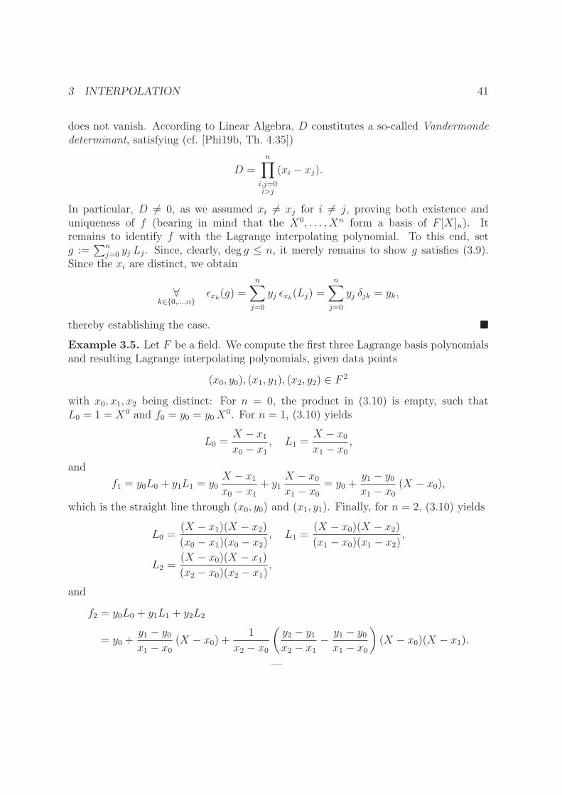
Example 3.5. Let F be a field. We compute the first three Lagrange basis polynomialsand resulting Lagrange interpolating polynomials, given data points
(x0, y0), (x1, y1), (x2, y2) ∈ F 2
with x0, x1, x2 being distinct: For n = 0, the product in (3.10) is empty, such thatL0 = 1 = X0 and f0 = y0 = y0X
0. For n = 1, (3.10) yields
L0 =X − x1x0 − x1
, L1 =X − x0x1 − x0
,
and
f1 = y0L0 + y1L1 = y0X − x1x0 − x1
+ y1X − x0x1 − x0
= y0 +y1 − y0x1 − x0
(X − x0),
which is the straight line through (x0, y0) and (x1, y1). Finally, for n = 2, (3.10) yields
L0 =(X − x1)(X − x2)(x0 − x1)(x0 − x2)
, L1 =(X − x0)(X − x2)(x1 − x0)(x1 − x2)
,
L2 =(X − x0)(X − x1)(x2 − x0)(x2 − x1)
,
and
f2 = y0L0 + y1L1 + y2L2
= y0 +y1 − y0x1 − x0
(X − x0) +1
x2 − x0
(y2 − y1x2 − x1
− y1 − y0x1 − x0
)(X − x0)(X − x1).
—

3 INTERPOLATION 42
The above formulas for f0, f1, f2 indicate that the interpolating polynomial can be builtrecursively, and we will see below (cf. (3.20a)) that this is, indeed, the case. Having arecursive formula at hand can be advantageous in many circumstances. For example,even though the complexity of building the interpolating polynomial from scratch isO(n2) in either case, if one already has the interpolating polynomial for x0, . . . , xn, then,using the recursive formula (3.20a) below, one obtains the interpolating polynomial forx0, . . . , xn, xn+1 in just O(n) steps.
Looking at the structure of f2 above, one sees that, while the first coefficient is just y0, thesecond one is a difference quotient (which, for F = R, can be seen as an approximationof some derivative y′(x)), and the third coefficient is a difference quotient of differencequotients (which, for F = R, can be seen as an approximation of some second derivativey′′(x)). Such iterated difference quotients are called divided differences and we will see inTh. 3.17 below that the same structure does, indeed, hold for interpolating polynomialsof all orders. However, we will first introduce and study a slightly more general formof polynomial interpolation, so-called Hermite interpolation, where the given pointsx0, . . . , xn no longer need to be distinct.
3.2.3 Hermite Interpolation
So far, we have determined an interpolating polynomial f of degree at most n fromvalues at n + 1 distinct points x0, . . . , xn ∈ F . Alternatively, one can prescribe thevalues of f at less than n + 1 points and, instead, additionally prescribe the values ofderivatives of f (cf. Def. 3.6 below) at some of the same points, where the total numberof pieces of data still needs to be n+1. For example, to determine f ∈ R[X] of degree atmost 7, one can prescribe f(1), f(2), f ′(2), f(3), f ′(3), f ′′(3), f ′′′(3), and f (4)(3). Onethen says that x1 = 2 is considered with multiplicity 2 and x2 = 3 is considered withmultiplicity 5. This particular kind of polynomial interpolation is known as Hermiteinterpolation.
While one is probably most familiar with the derivative as an analytic concept (e.g.for functions from R into R), for polynomials, one can define the derivative in entirelyalgebraic terms:
Definition 3.6. Let F be a field. Let n ∈ N0 and f0, . . . , fn ∈ F . For f =∑n
i=0 fiXi ∈
F [X], we define the derivative f ′ ∈ F [X] of f by letting
f ′ := 0 for n = 0, f ′ :=n−1∑
i=0
(i+ 1) fi+1Xi for n ≥ 1.
Higher derivatives are defined recursively, in the usual way, by letting
f (0) := f, ∀k∈N0
f (k+1) := (f (k))′,

3 INTERPOLATION 43
and we make use of the notation f ′′ := f (2), f ′′′ := f (3).
Proposition 3.7. Let F be a field.
(a) Forming the derivative in F [X] is linear, i.e.
∀f,g∈F [X]
∀λ,µ∈F
(λf + µg)′ = λf ′ + µg′.
(b) Forming the derivative in F [X] satisfies the product rule, i.e.
∀f,g∈F [X]
(fg)′ = f ′g + fg′.
(c) For each x ∈ F and each n ∈ N, one has
((X − x)n
)′= n (X − x)n−1.
(d) Forming higher derivatives in F [X] satisfies the general Leibniz rule, i.e.
∀n∈N0
∀f,g∈F [X]
(fg)(n) =n∑
k=0
(n
k
)f (n−k)g(k).
(e) For each x ∈ F , one has, setting g(−1) := 0,
∀n∈N0
∀g∈F [X]
((X − x) g
)(n)= n g(n−1) + (X − x) g(n).
Proof. Exercise. �
Theorem 3.8. Let F be a field, n ∈ N, and assume charF = 0 or charF ≥ n (i.e., inF , k ·1 6= 0 for each k ∈ {1, . . . , n−1}, cf. [Phi19a, Def. and Rem. 4.43]). Let f ∈ F [X]with deg f = n, x ∈ F . If m ∈ {0, . . . , n− 1} and, using the notation of (3.7),
f(x) = f ′(x) = · · · = f (m)(x) = 0, (3.11)
then x is a zero of multiplicity at least m+ 1 for f , i.e. (cf. [Phi19b, Cor. 7.14])
∃q∈F [X]
(deg q = n−m− 1 ∧ f = q (X − x)m+1
).
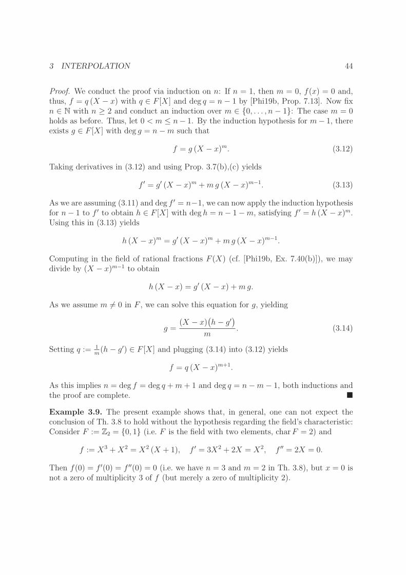
3 INTERPOLATION 44
Proof. We conduct the proof via induction on n: If n = 1, then m = 0, f(x) = 0 and,thus, f = q (X − x) with q ∈ F [X] and deg q = n− 1 by [Phi19b, Prop. 7.13]. Now fixn ∈ N with n ≥ 2 and conduct an induction over m ∈ {0, . . . , n − 1}: The case m = 0holds as before. Thus, let 0 < m ≤ n− 1. By the induction hypothesis for m− 1, thereexists g ∈ F [X] with deg g = n−m such that
f = g (X − x)m. (3.12)
Taking derivatives in (3.12) and using Prop. 3.7(b),(c) yields
f ′ = g′ (X − x)m +mg (X − x)m−1. (3.13)
As we are assuming (3.11) and deg f ′ = n−1, we can now apply the induction hypothesisfor n− 1 to f ′ to obtain h ∈ F [X] with deg h = n− 1−m, satisfying f ′ = h (X − x)m.Using this in (3.13) yields
h (X − x)m = g′ (X − x)m +mg (X − x)m−1.
Computing in the field of rational fractions F (X) (cf. [Phi19b, Ex. 7.40(b)]), we maydivide by (X − x)m−1 to obtain
h (X − x) = g′ (X − x) +mg.
As we assume m 6= 0 in F , we can solve this equation for g, yielding
g =(X − x)
(h− g′
)
m. (3.14)
Setting q := 1m(h− g′) ∈ F [X] and plugging (3.14) into (3.12) yields
f = q (X − x)m+1.
As this implies n = deg f = deg q +m+ 1 and deg q = n−m− 1, both inductions andthe proof are complete. �
Example 3.9. The present example shows that, in general, one can not expect theconclusion of Th. 3.8 to hold without the hypothesis regarding the field’s characteristic:Consider F := Z2 = {0, 1} (i.e. F is the field with two elements, charF = 2) and
f := X3 +X2 = X2 (X + 1), f ′ = 3X2 + 2X = X2, f ′′ = 2X = 0.
Then f(0) = f ′(0) = f ′′(0) = 0 (i.e. we have n = 3 and m = 2 in Th. 3.8), but x = 0 isnot a zero of multiplicity 3 of f (but merely a zero of multiplicity 2).

3 INTERPOLATION 45
Theorem 3.10 (Hermite Interpolation). Let F be a field and r, n ∈ N0. Let x0, . . . , xr ∈F be r+1 distinct elements of F . Moreover, let m0, . . . ,mr ∈ N be such that
∑rk=0mk =
n+ 1 and assume y(m)j ∈ F for each j ∈ {0, . . . , r}, m ∈ {0, . . . ,mj − 1}.
(a) The map
A : F [X]n −→ F n+1,
A(p) :=(p(x0), . . . , p
(m0−1)(x0), . . . , p(xr), . . . , p(mr−1)(xr)
).
is linear.
(b) Assume charF = 0 or charF ≥ M := max{m0, . . . ,mr}. Then there exists aunique polynomial f ∈ F [X]n (i.e. of degree at most n) such that (using the notationof (3.7))
f (m)(xj) = y(m)j for each j ∈ {0, . . . , r}, m ∈ {0, . . . ,mj − 1}. (3.15)
Proof. (a): If p, q ∈ F [X]n and λ, µ ∈ F , then
A(λp+ µq) =(. . . , (λp+ µq)(l)(xk), . . .
) Prop. 3.7(a)=
(. . . , (λp(l) + µq(l))(xk), . . .
)
=(. . . , λp(l)(xk) + µq(l)(xk), . . .
)
= λ(. . . , p(l)(xk), . . .
)+ µ
(. . . , q(l)(xk), . . .
)= λA(p) + µA(q),
proving the linearity of A.
(b): The existence and uniqueness statement of the theorem is the same as saying thatthe map A of (a) is bijective. Since A is linear by (a) and since dimF [X]n = dimF n+1 =n+ 1, it suffices to show that A is injective, i.e. kerA = {0}. If A(p) = (0, . . . , 0), then,by Th. 3.8, each xk is a zero of p with multiplicity at least mk, such that p has at leastn+ 1 zeros. More precisely, Th. 3.8 implies that, if p 6= 0, then the prime factorizationof p (cf. [Phi19b, Cor. 7.37]) must contain the factor
∏rk=0(X− xk)mk , i.e. deg p ≥ n+1.
Since deg p ≤ n, we know p = 0, showing kerA = {0}, thereby completing the proof. �
Example 3.11. The present example shows that, in general, one can not expect theconclusion of Th. 3.10(b) to hold without the hypothesis regarding the field’s character-istic: We show that, for F := Z2 = {0, 1}, the Hermite interpolation problem can havemultiple solutions or no solutions: The 4 conditions
f(0) = f ′(0) = f ′′(0) = 0, f(1) = 0
are all satisfied by both f = 0 ∈ F [X]3 and by f = X3 +X2 ∈ F [X]3 (cf. Ex. 3.9). Onthe other hand, since (X3)′ = 3X2 = X2 and (X2)′ = 2X = 0, one has f ′′ = 0 for eachf ∈ F [X]3, i.e. the 4 conditions
f(0) = f ′(0) = f ′′(0) = 1, f(1) = 0

3 INTERPOLATION 46
are not satisfied by any f ∈ F [X]3.
Definition 3.12. As in Th. 3.10, let F be a field and r, n ∈ N0; let x0, . . . , xr ∈ F ber + 1 distinct elements of F ; let m0, . . . ,mr ∈ N be such that
∑rk=0mk = n + 1; and
assume y(m)j ∈ F for each j ∈ {0, . . . , r}, m ∈ {0, . . . ,mj − 1}. Also, as in Th. 3.10(b),
assume charF = 0 or charF ≥M := max{m0, . . . ,mr}. Finally, let (x0, . . . , xn) ∈ F n+1
be such that, for each k ∈ {0, . . . , r}, preciselymk of the xj are equal to xk (i.e. xk occursprecisely mk times in the vector (x0, . . . , xn)).
(a) Let P [x0, . . . , xn] := f ∈ F [X]n denote the unique interpolating polynomial satisfy-
ing (3.15). As a caveat, we note that P [x0, . . . , xn] also depends on the y(m)j , which
is, however, suppressed in the notation.
(b) If x0, . . . , xn are all distinct (i.e. n = r and (x0, . . . , xn) constitutes a permutationof (x0, . . . , xr)) and g : F −→ F is a function such that
∀j∈{0,...,n}
g(xj) = y(0)j ,
then we define the additional notation
P [g|x0, . . . , xn] := P [x0, . . . , xn].
(c) Let F = R with a, b ∈ R, a < b, such that x0, . . . , xr ∈ [a, b], and let g : [a, b] −→ R
be an M times differentiable function such that
g(m)(xj) = y(m)j for each j ∈ {0, . . . , r}, m ∈ {0, . . . ,mj − 1}.
Then, as in (b), we define the additional notation
P [g|x0, . . . , xn] := P [x0, . . . , xn].
—
We remain in the situation of Def. 3.12 and denote the interpolating polynomial byf := P [x0, . . . , xn]. If one is only interested in the value f(x) for some x ∈ F , ratherthan all the coefficients of f (or rather than evaluating f at many different elements ofF ), then an efficient way to obtain f(x) is by means of a so-called Neville tableau (cf.Rem. 3.14 below), making use of the recursion provided by the following Th. 3.13(a).
Theorem 3.13. We consider the situation of Def. 3.12.

3 INTERPOLATION 47
(a) The interpolating polynomials satisfy the following recursion: For r = 0, one has
P [x0, . . . , xn] = P [x0, . . . , x0] =n∑
j=0
(X − x0)jj!
y(j)0 . (3.16a)
For r > 0, one has, for each k, l ∈ {0, . . . , n} such that xk 6= xl,
P [x0, . . . , xn] =(X − xl)P [x0, . . . , xl, . . . , xn]− (X − xk)P [x0, . . . , xk, . . . , xn]
xk − xl(3.16b)
(the hatted symbols xl and xk mean that the corresponding arguments are omitted).
(b) The interpolating polynomials do not depend on the order of the x0, . . . , xn ∈ F ,i.e., for each permutation π on {0, . . . , n},
P [xπ(0), . . . , xπ(n)] = P [x0, . . . , xn].
Proof. (a): The case r = 0 holds, since, clearly,
∀k∈N0
((X − x0)j
j!
)(k)
(x0) =
0 for k < j,
1 for k = j,
0 for k > j,
implying
∀m∈{0,...,n}
(n∑
j=0
(X − x0)jj!
y(j)0
)(m)
(x0) = y(m)0 .
We now consider the case r > 0. Letting p := P [x0, . . . , xn] and letting q denote thepolynomial given by the right-hand side of (3.16b), we have to show p = q. Clearly,both p and q are in F [X]n. Thus, the proof is complete, if we can show that q alsosatisfies (3.15), i.e.
q(m)(xj) = y(m)j for each j ∈ {0, . . . , r}, m ∈ {0, . . . ,mj − 1}. (3.17)
To verify (3.17), given k, l ∈ {0, . . . , n} with xk 6= xl, we use Prop. 3.7(e) to obtain, foreach m ∈ N0,
q(m) =mP [x0, . . . , xl, . . . , xn]
(m−1) + (X − xl)P [x0, . . . , xl, . . . , xn](m)
xk − xl− mP [x0, . . . , xk, . . . , xn]
(m−1) + (X − xk)P [x0, . . . , xk, . . . , xn](m)
xk − xl. (3.18)

3 INTERPOLATION 48
Now we fix j ∈ {0, . . . , r} such that xj = xk and let m ∈ {0, . . . ,mj − 1}. Then (setting
y(−1)j := 0)
q(m)(xj) =my
(m−1)j + (xk − xl) y(m)
j −my(m−1)j − 0
xk − xl= y
(m)j .
Similarly, for j ∈ {0, . . . , r} such that xj = xl:
q(m)(xj) =my
(m−1)j + 0−my
(m−1)j − (xl − xk) y(m)
j
xk − xl= y
(m)j .
Finally, if j ∈ {0, . . . , r} is such that xj /∈ {xk, xl}, then
q(m)(xj) =my
(m−1)j + (xj − xl) y(m)
j −my(m−1)j − (xj − xk) y(m)
j
xk − xl= y
(m)j ,
proving that (3.17) does, indeed, hold.
(b) holds due to the fact that the interpolating polynomial P [x0, . . . , xn] is determinedby the conditions (3.15), which do not depend on the order of x0, . . . , xn (according toDef. 3.12, this order independence of the interpolating polynomial is already built intothe definition of P [x0, . . . , xn]). �
Remark 3.14. To use the recursion (3.16), to compute P [x0, . . . , xn](x) for x ∈ F , wenow assume that (x0, . . . , xn) is ordered in such a way that identical entries are adjacent:
(x0, . . . , xn) = (x0, . . . , x0, x1, . . . , x1, . . . , xr, . . . , xr). (3.19)
Moreover, for fixed x ∈ F , we now define
∀α,β∈{0,...,n},
α≥β
Pαβ := P [xα−β, . . . , xα](x).
Then Pnn = P [x0, . . . , xn](x) is the desired value. According to Th. 3.13(a) and (3.19),
Pαβ =m∑
k=0
(x− xj)kk!
y(k)j for xα−β = xα = xj and m = β,
Pαβ =(x− xα−β)P [x1+α−β, . . . , xα](x)− (x− xα)P [xα−β, . . . , xα−1](x)
xα − xα−β
=(x− xα−β)Pα,β−1 − (x− xα)Pα−1,β−1
xα − xα−β
for xα−β 6= xα.

3 INTERPOLATION 49
In consequence, Pnn can be computed, in O(n2) steps, via the following Neville tableau:
y(0)0 = P00
ցy(0)0 = P10 → P11
ց ցy(0)0 = P20 → P21 → P22
......
.... . .
y(0)r = Pn−1,0 → Pn−1,1 → . . . . . .Pn−1,n−1
ց ց ցy(0)r = Pn0 → Pn1 → . . . . . . Pn,n−1 → Pnn
Example 3.15. Consider a field F with charF 6= 2, n := 4, r := 1, and let
x0 := 1, x1 := 2,
y0 := 1, y′0 := 4, y1 := 3, y′1 := 1, y′′1 := 2.
Setting x := 3, we want to compute P44 = P [1, 1, 2, 2, 2](3), using a Neville tableauaccording to Rem. 3.14. In preparation, we compute
P [1, 1](3) = y0 + (3− 1) y(1)0 = 1 + 2 · 4 = 9,
P [2, 2](3) = y1 + (3− 2) y(1)1 = 3 + 1 = 4,
P [2, 2, 2](3) = P [2, 2](3) +(3− 2)2
2!y(2)1 = 4 + 1 = 5.
Thus, we obtain the Neville tableau
P00 = y0 = 1ց
P10 = y0 = 1 → P11 = P [1, 1](3) = 9ց ց
P20 = y1 = 3 → P21 = P [1, 2](3) = (3−1)·3−(3−2)·12−1 = 5 → P22 = P [1, 1, 2](3) = 2·5−9
2−1 = 1
ց ցP30 = y1 = 3 → P31 = P [2, 2](3) = 4 → P32 = P [1, 2, 2](3) = 2·4−5
2−1 = 3
ց ցP40 = y1 = 3 → P41 = P [2, 2](3) = 4 → P42 = P [2, 2, 2](3) = 5
and, continued:
. . . P22 = 1ց
. . . P32 = 3 → P33 = P [1, 1, 2, 2](3) = 2·3−12−1 = 5
ց ց. . . P42 = 5 → P43 = P [1, 2, 2, 2](3) = 2·5−3
2−1 = 7 → P44 = P [1, 1, 2, 2, 2](3) = 2·7−52−1 = 9.

3 INTERPOLATION 50
3.2.4 Divided Differences and Newton’s Interpolation Formula
We now come back to the divided differences mentioned at the end of Sec. 3.2.2. Weproceed to immediately define divided differences in the general context of Hermiteinterpolation:
Definition 3.16. As in Def. 3.12, let F be a field and r, n ∈ N0; let x0, . . . , xr ∈ F ber + 1 distinct elements of F ; let m0, . . . ,mr ∈ N be such that
∑rk=0mk = n + 1; and
assume y(m)j ∈ F for each j ∈ {0, . . . , r}, m ∈ {0, . . . ,mj − 1}; assume charF = 0 or
charF ≥ M := max{m0, . . . ,mr}; and let (x0, . . . , xn) ∈ F n+1 be such that, for eachk ∈ {0, . . . , r}, precisely mk of the xj are equal to xk (i.e. xk occurs precisely mk timesin the vector (x0, . . . , xn)).
(a) We write the interpolating polynomial f := P [x0, . . . , xn] ∈ F [X]n in the formf =
∑ni=0 aiX
i with a0, . . . , an ∈ F . The value
[x0, . . . , xn] := an ∈ F
is called a divided difference of nth order (as P [x0, . . . , xn], it is determined by the
xj together with the y(m)j , but, once again, the dependence on the y
(m)j is suppressed
in the notation).
(b) If x0, . . . , xn are all distinct (i.e. n = r and (x0, . . . , xn) constitutes a permutationof (x0, . . . , xr)) and g : F −→ F is a function such that
∀j∈{0,...,n}
g(xj) = y(0)j ,
then we define the additional notation
[g|x0, . . . , xn] := [x0, . . . , xn].
(c) Let F = R with a, b ∈ R, a < b, such that x0, . . . , xr ∈ [a, b], and let g : [a, b] −→ R
be an M times differentiable function such that
g(m)(xj) = y(m)j for each j ∈ {0, . . . , r}, m ∈ {0, . . . ,mj − 1}.
Then, as in (b), we define the additional notation
[g|x0, . . . , xn] := [x0, . . . , xn].

3 INTERPOLATION 51
Theorem 3.17. In the situation of Def. 3.16, the interpolating polynomial P [x0, . . . , xn]∈ F [X]n can be written in the following form known as Newton’s divided differenceinterpolation formula:
P [x0, . . . , xn] =n∑
j=0
[x0, . . . , xj ]ωj, (3.20a)
where, for each j ∈ {0, 1, . . . , n},
ωj :=
j−1∏
i=0
(X − xi) ∈ F [X]j ⊆ F [X]n (3.20b)
are the so-called Newton basis polynomials. In particular, (3.20a) means that the inter-polating polynomials satisfy the recursive relation
P [x0] = y(0)0 , (3.21a)
P [x0, . . . , xj ] = P [x0, . . . , xj−1] + [x0, . . . , xj ]ωj for 1 ≤ j ≤ n. (3.21b)
Proof. We conduct the proof via induction on n ∈ N0: Noting ω0 = 1 (empty product),the base case (n = 0) is provided by the true statement
P [x0] = y(0)0 = [x0]ω0.
Now let n > 0. Then, according to Def. 3.16, there exist a0, . . . , an−1 ∈ F and q ∈F [X]n−1 such that
p := P [x0, . . . , xn] = [x0, . . . , xn]Xn +
n−1∑
i=0
aiXi = [x0, . . . , xn]ωn + q.
Thus, q = p− [x0, . . . , xn]ωn and, to show q = pn−1 := P [x0, . . . , xn−1], we need to showq satisfies
q(m)(xj) = y(m)j for each j ∈ {0, . . . , r} \ {j0}, m ∈ {0, . . . ,mj − 1}, (3.22a)
q(m)(xj0) = y(m)j0
for each m ∈ {0, . . . ,mj0 − 1} \ {mj0 − 1}, (3.22b)
where j0 ∈ {0, . . . , r} is such that xn = xj0 . However, q does satisfy (3.22), since(3.22) is satisfied with q replaced by p and, by (3.20b) in combination with Prop. 3.7(d),
ω(m)n (xj) = 0 for each j ∈ {0, . . . , r} \ {j0} and each m ∈ {0, . . . ,mj − 1}, as well as for
each m ∈ {0, . . . ,mj0 − 1} \ {mj0 − 1} for j = j0. Thus, q = pn−1, showing
p = [x0, . . . , xn]ωn + q = [x0, . . . , xn]ωn + pn−1ind.hyp.= [x0, . . . , xn]ωn +
n−1∑
j=0
[x0, . . . , xj ]ωj ,
thereby completing the induction. �

3 INTERPOLATION 52
We can now make use of our knowledge regarding interpolating polynomials to inferproperties of the divided differences (in particular, we will see that divided differencescan also be efficiently computed using Neville tableaus):
Theorem 3.18. In the situation of Def. 3.16, the divided differences satisfy the follow-ing:
(a) Recursion: For r = 0, one has
[x0, . . . , xn] = [x0, . . . , x0] =y(n)0
n!. (3.23a)
For r > 0, one has, for each k, l ∈ {0, . . . , n} such that xk 6= xl,
[x0, . . . , xn] =[x0, . . . , xl, . . . , xn]− [x0, . . . , xk, . . . , xn]
xk − xl(3.23b)
(where, as before, the hatted symbols xl and xk mean that the corresponding argu-ments are omitted).
(b) [x0, . . . , xn] does not depend on the order of the x0, . . . , xn ∈ F , i.e., for each per-mutation π on {0, . . . , n},
[xπ(0), . . . , xπ(n)] = [x0, . . . , xn].
Proof. (a): Case r = 0: According to (3.16a), we have
P [x0, . . . , xn] = P [x0, . . . , x0] =n∑
j=0
(X − x0)jj!
y(j)0 ,
i.e. the coefficient of Xn isy(n)0
n!. Case r > 0: According to (3.16b), we have, for each
k, l ∈ {0, . . . , n} such that xk 6= xl,
P [x0, . . . , xn] =(X − xl)P [x0, . . . , xl, . . . , xn]− (X − xk)P [x0, . . . , xk, . . . , xn]
xk − xl,
where, comparing the coefficient of Xn on the left-hand side with the coefficient of Xn
on the right-hand side immediately proves (3.23b).
(b) is immediate from Th. 3.13(b). �
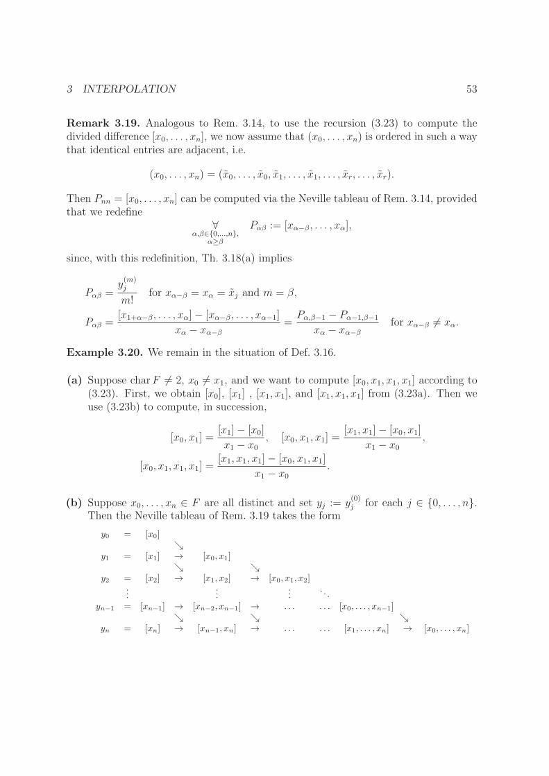
3 INTERPOLATION 53
Remark 3.19. Analogous to Rem. 3.14, to use the recursion (3.23) to compute thedivided difference [x0, . . . , xn], we now assume that (x0, . . . , xn) is ordered in such a waythat identical entries are adjacent, i.e.
(x0, . . . , xn) = (x0, . . . , x0, x1, . . . , x1, . . . , xr, . . . , xr).
Then Pnn = [x0, . . . , xn] can be computed via the Neville tableau of Rem. 3.14, providedthat we redefine
∀α,β∈{0,...,n},
α≥β
Pαβ := [xα−β, . . . , xα],
since, with this redefinition, Th. 3.18(a) implies
Pαβ =y(m)j
m!for xα−β = xα = xj and m = β,
Pαβ =[x1+α−β, . . . , xα]− [xα−β, . . . , xα−1]
xα − xα−β
=Pα,β−1 − Pα−1,β−1
xα − xα−β
for xα−β 6= xα.
Example 3.20. We remain in the situation of Def. 3.16.
(a) Suppose charF 6= 2, x0 6= x1, and we want to compute [x0, x1, x1, x1] according to(3.23). First, we obtain [x0], [x1] , [x1, x1], and [x1, x1, x1] from (3.23a). Then weuse (3.23b) to compute, in succession,
[x0, x1] =[x1]− [x0]
x1 − x0, [x0, x1, x1] =
[x1, x1]− [x0, x1]
x1 − x0,
[x0, x1, x1, x1] =[x1, x1, x1]− [x0, x1, x1]
x1 − x0.
(b) Suppose x0, . . . , xn ∈ F are all distinct and set yj := y(0)j for each j ∈ {0, . . . , n}.
Then the Neville tableau of Rem. 3.19 takes the form
y0 = [x0]ց
y1 = [x1] → [x0, x1]ց ց
y2 = [x2] → [x1, x2] → [x0, x1, x2]...
......
. . .
yn−1 = [xn−1] → [xn−2, xn−1] → . . . . . . [x0, . . . , xn−1]ց ց ց
yn = [xn] → [xn−1, xn] → . . . . . . [x1, . . . , xn] → [x0, . . . , xn]

3 INTERPOLATION 54
(c) As in Ex. 3.15, consider a field F with charF 6= 2, n := 4, r := 1, and the givendata
x0 = 1, x1 = 2,
y0 = 1, y′0 = 4, y1 = 3, y′1 = 1, y′′1 = 2.
This time, we seek to obtain the complete interpolating polynomial P [1, 1, 2, 2, 2],using Newton’s interpolation formula (3.20a):
P [1, 1, 2, 2, 2] = [1] + [1, 1](X − 1) + [1, 1, 2](X − 1)2 + [1, 1, 2, 2](X − 1)2(X − 2)
+ [1, 1, 2, 2, 2](X − 1)2(X − 2)2. (3.24)
The coefficients can be computed from the Neville tableau given by Rem. 3.19:
[1] = y0 = 1ց
[1] = y0 = 1 → [1, 1] = y′0 = 4ց ց
[2] = y1 = 3 → [1, 2] = 3−12−1 = 2 → [1, 1, 2] = 2−4
2−1 = −2ց ց ց
[2] = y1 = 3 → [2, 2] = y′1 = 1 → [1, 2, 2] = 1−22−1 = −1 → [1, 1, 2, 2] = −1−(−2)
2−1 = 1
ց ց ց[2] = y1 = 3 → [2, 2] = y′1 = 1 → [2, 2, 2] =
y′′
1
2! = 1 → [1, 2, 2, 2] = 1−(−1)2−1 = 2
and, finally,. . . [1, 1, 2, 2] = 1
ց. . . [1, 2, 2, 2] = 2 → [1, 1, 2, 2, 2] = 2−1
2−1 = 1.
Hence, plugging the results of the tableau into (3.24),
P [1, 1, 2, 2, 2] = 1 + 4(X − 1)− 2(X − 1)2 + (X − 1)2(X − 2) + (X − 1)2(X − 2)2.
—
Additional formulas for divided differences over a general field F can be found in Ap-pendix D. Here, we now proceed to present a result for the field F = R, where thereturns out to be a surprising relation between divided differences and integrals over sim-plices. We start with some preparations:
Notation 3.21. For n ∈ N, the following notation is introduced:
Σn :=
{(s1, . . . , sn) ∈ Rn :
n∑
i=1
si ≤ 1 and 0 ≤ si for each i ∈ {1, . . . , n}}.
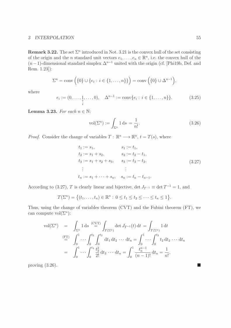
3 INTERPOLATION 55
Remark 3.22. The set Σn introduced in Not. 3.21 is the convex hull of the set consistingof the origin and the n standard unit vectors e1, . . . , en ∈ Rn, i.e. the convex hull of the(n−1)-dimensional standard simplex ∆n−1 united with the origin (cf. [Phi19b, Def. andRem. 1.23]):
Σn = conv({0} ∪ {ei : i ∈ {1, . . . , n}}
)= conv
({0} ∪∆n−1
),
whereei := (0, . . . , 1
↑i
, . . . , 0), ∆n−1 := conv{ei : i ∈ {1, . . . , n}}. (3.25)
Lemma 3.23. For each n ∈ N:
vol(Σn) :=
∫
Σn
1 ds =1
n!. (3.26)
Proof. Consider the change of variables T : Rn −→ Rn, t = T (s), where
t1 := s1,
t2 := s1 + s2,
t3 := s1 + s2 + s3,
...
tn := s1 + · · ·+ sn,
s1 := t1,
s2 := t2 − t1,s3 := t3 − t2,...
sn := tn − tn−1.
(3.27)
According to (3.27), T is clearly linear and bijective, det JT−1 ≡ detT−1 = 1, and
T (Σn) ={(t1, . . . , tn) ∈ Rn : 0 ≤ t1 ≤ t2 ≤ · · · ≤ tn ≤ 1
}.
Thus, using the change of variables theorem (CVT) and the Fubini theorem (FT), wecan compute vol(Σn):
vol(Σn) =
∫
Σn
1 ds(CVT)=
∫
T (Σn)
det JT−1(t) dt =
∫
T (Σn)
1 dt
(FT)=
∫ 1
0
· · ·∫ t3
0
∫ t2
0
dt1 dt2 · · · dtn =
∫ 1
0
· · ·∫ t3
0
t2 dt2 · · · dtn
=
∫ 1
0
· · ·∫ t4
0
t232!
dt3 · · · dtn =
∫ 1
0
tn−1n
(n− 1)!dtn =
1
n!,
proving (3.26). �

3 INTERPOLATION 56
Theorem 3.24 (Hermite-Genocchi Formula). Consider the situation of Def. 3.16(c),i.e. r, n ∈ N0 with x0, . . . , xr ∈ [a, b] ⊆ R distinct (a, b ∈ R, a < b); m0, . . . ,mr ∈ N
such that∑r
k=0mk = n + 1 and g ∈ Cn[a, b] (this assumption is actually stronger thanin Def. 3.16(c)) with
g(m)(xj) = y(m)j ∈ R for each j ∈ {0, . . . , r}, m ∈ {0, . . . ,mj − 1};
and (x0, . . . , xn) ∈ Rn+1 such that, for each k ∈ {0, . . . , r}, precisely mk of the xj areequal to xk. Then the divided differences satisfy the following relation, known as theHermite-Genocchi formula:
n ≥ 1 ⇒ [g|x0, . . . , xn] =∫
Σn
g(n)
(x0 +
n∑
i=1
si(xi − x0))
ds , (3.28)
where Σn is the set according to Not. 3.21.
Proof. First, note that, for each s ∈ Σn,
a = x0 + a− x0 ≤ x0 +n∑
i=1
si(a− x0) ≤ xs := x0 +n∑
i=1
si(xi − x0)
≤ x0 +n∑
i=1
si(b− x0) ≤ x0 + b− x0 = b,
such that g(n) is defined at xs. Moreover, the integral in (3.28) exists, as the continuousfunction g(n) is bounded on the compact set Σn. If r = 0 (i.e. x0 = · · · = xn = x0), then
∫
Σn
g(n)
(x0 +
n∑
i=1
si(xi − x0))
ds =
∫
Σn
g(n)(x0) ds(3.26)=
g(n)(x0)
n!
=y(n)0
n!
(3.23a)= [g|x0, . . . , xn],
proving (3.28) in this case. For r > 0, we prove (3.28) via induction on n ∈ N, where,by Th. 3.18(b), we may assume x0 6= xn. Then, for n = 1, (3.28) is an easy consequenceof the fundamental theorem of calculus (FTC) (note Σ1 = [0, 1]):
∫ 1
0
g′(x0 + s(x1 − x0)
)ds =
[g(x0 + s(x1 − x0)
)
x1 − x0
]1
0
=g(x1)− g(x0)x1 − x0
=y1 − y0x1 − x0
= [g|x0, x1].

3 INTERPOLATION 57
Next, for the induction step, let n ∈ N and compute
∫
Σn+1
g(n+1)
(x0 +
n+1∑
i=1
si(xi − x0)
)ds
Fubini=
∫
Σn
(∫ 1−∑ni=1 si
0g(n+1)
(x0 +
n∑
i=1
si(xi − x0) + sn+1(xn+1 − x0)
)dsn+1
)d(s1, . . . , sn)
FTC=
1
xn+1 − x0
∫
Σn
(g(n)
(xn+1 +
n∑
i=1
si(xi − xn+1)
)
−g(n)(x0 +
n∑
i=1
si(xi − x0)
))d(s1, . . . , sn)
ind.hyp.=
[g|x1, . . . , xn+1]− [g|x0, . . . , xn]xn+1 − x0
(3.23b)= [g|x0, . . . , xn+1],
thereby establishing the case. �
Theorem 3.25. Under the assumptions of Th. 3.24 and letting p := P [g|x0, . . . , xn] ∈R[X]n be the corresponding interpolating polynomial (cf. Def. 3.12(c)), the followingholds true:
(a) For each x ∈ [a, b]:
g(x) = p(x) + [g|x, x0, . . . , xn]ωn+1(x), (3.29)
where
ωn+1 =n∏
i=0
(X − xi)
(if x = x0 = · · · = xn, then [g|x, x0, . . . , xn] is only defined if g is (n + 1) timesdifferentiable – however, in this case, ωn+1(x) = 0 and g(x) = p(x) still holds, evenif [g|x, x0, . . . , xn] is not defined).
(b) (Mean Value Theorem for Divided Differences) Given x ∈ [a, b], let
m := min{x, x0, . . . , xn}, M := max{x, x0, . . . , xn}.If g ∈ Cn+1[a, b], then there exists ξ = ξ(x, x0, . . . , xn) ∈ [m,M ] such that
[g|x, x0, . . . , xn] =g(n+1)(ξ)
(n+ 1)!. (3.30)
In consequence, with ωn+1 as in (a), one then also has
g(x) = p(x) +g(n+1)(ξ)
(n+ 1)!ωn+1(x). (3.31)

3 INTERPOLATION 58
(c) The function
δ : [a, b]n+1 −→ R, (x0, . . . , xn) 7→ [g|x0, . . . , xn],
is continuous, in particular, continuous in each xk, k ∈ {0, . . . , n}. In consequence,if ξ(x, x0, . . . , xn) is chosen as in (b), then the map
(x0, . . . , xn) 7→ g(n+1)(ξ(x, x0, . . . , xn)
)
is continuous on [a, b]n+1.
Proof. (a): For x ∈ [a, b], one obtains:
p(x) + [g|x, x0, . . . , xn]ωn+1(x)(3.20)=
n∑
j=0
[g|x0, . . . , xj]ωj(x) + [g|x0, . . . , xn, x]ωn+1(x)
(3.20)= g(x).
(b): If x = x0 = · · · = xn, then (3.30) holds due to
[g|x, x0, . . . , xn](3.23a)=
y(n+1)0
(n+ 1)!=g(n+1)(x0)
(n+ 1)!.
Otherwise, we can apply Th. 3.24 with a, b replaced by m,M . Using (3.28) togetherwith the mean value theorem of integration (see, e.g., [Phi17, Th. 2.16(f)]) then yieldsξ ∈ [m,M ] such that
[g|x, x0, . . . , xn] = g(n+1)(ξ)
∫
Σn+1
1 ds(3.26)=
g(n+1)(ξ)
(n+ 1)!,
proving (3.30). Plugging (3.30) into (3.29) yields (3.31).
(c): For n = 0, the continuity of x0 7→ [g|x0] = g(x0) is merely the assumed continuityof g. Let n > 0. Since g(n) is continuous and the continuous function |g(n)| is uniformlybounded on the compact interval [a, b], the continuity of δ is due to (3.28) and thecontinuity of parameter-dependent integrals (see, e.g., [Phi17, Th. 2.22]). �
3.2.5 Convergence and Error Estimates
We will now provide a convergence result for the approximation of a (benign) C∞
function by interpolating polynomial functions. Recall from Def. and Rem. 3.3(b) that,given f ∈ R[X], φ(f) ∈ Pol(R), φ(f)(x) = f(x), is the corresponding polynomialfunction.

3 INTERPOLATION 59
Theorem 3.26. As in Th. 3.24, let a, b ∈ R, a < b. Let g ∈ C∞[a, b] and consider asequence (xk)k∈N0 in [a, b]. For each n ∈ N, define pn := P [g|x0, . . . , xn] ∈ R[X]n to bethe interpolating polynomial corresponding to the first n+ 1 points – thus, according toTh. 3.17 and Th. 3.24,
∀n∈N
pn =n∑
j=0
[g|x0, . . . , xj]ωj ,
where
[g|x0, . . . , xj ] =∫
Σj
g(j)
(x0 +
j∑
i=1
si(xi − x0))
ds , ωj :=
j−1∏
i=0
(X − xi).
If there exist K,R ∈ R+0 such that
∀n∈N
‖g(n)‖∞ ≤ Kn!Rn, (3.32)
then one has the error estimate
∀n∈N0
∥∥g − φ(pn)∥∥∞ ≤
‖g(n+1)‖∞(n+ 1)!
∥∥φ(ωn+1)∥∥∞ ≤ KRn+1(b− a)n+1. (3.33)
If, moreover, R < (b− a)−1, then one also has the convergence
limn→∞
∥∥g − φ(pn)∥∥∞ = 0. (3.34)
Proof. The first estimate in (3.33) is merely (3.31), while the second estimate in (3.33)is (3.32) combined with ‖φ(ωn+1)‖∞ ≤ (b− a)n+1. As R < (b− a)−1, (3.33) establishes(3.34). �
Example 3.27. Suppose g ∈ C∞[a, b] is such that there exists C ≥ 0 satisfying
∀n∈N
‖g(n)‖∞ ≤ Cn. (3.35)
We claim that, in that case, there are K ∈ R+0 and 0 ≤ R < (b− a)−1 satisfying (3.32)
(in particular, this shows that Th. 3.26 applies to all functions of the form g(x) = ekx,g(x) = sin(kx), g(x) = cos(kx)). To verify that (3.35) implies (3.32), set R := 1
2(b−a)−1,
choose N ∈ N sufficiently large such that n! > (C/R)n for each n > N , and setK := max{(C/R)m : 0 ≤ m ≤ N}. Then, for each n ∈ N,
‖g(n)‖∞ ≤ Cn = (C/R)nRn ≤ K n!Rn.

3 INTERPOLATION 60
Remark 3.28. When approximating g ∈ C∞[a, b] by an interpolating polynomial pn,the accuracy of the approximation depends on the choice of the xj. If one choosesequally-spaced xj, then ωn+1(x) will be much larger in the vicinity of a and b than inthe center of the interval. This behavior of ωn+1 can be counteracted by choosing moredata points in the vicinity of a and b. This leads to the problem of finding data pointssuch that ‖φ(ωn+1)‖∞ is minimized. If a = −1, b = 1, then the optimal choice for thedata points is
xj := cos
(2j + 1
2n+ 2π
)for each j ∈ {0, . . . , n}.
These xj are precisely the zeros of the so-called Chebyshev polynomials, which we willstudy in Sec. 3.2.6 below (cf. Ex. 3.35).
—
One can compute n! [g|x0, . . . , xn] as a numerical approximation to g(n)(x). We obtainthe following error estimate:
Theorem 3.29 (Numerical Differentiation). Let a, b ∈ R, a < b, g ∈ Cn+1[a, b], n ∈ N0,x ∈ [a, b]. Then, given n + 1 (not necessarily distinct) points x0, . . . , xn ∈ [a, b] anddefining [g|x0, . . . , xn] as in Def. 3.16(c), the following estimate holds:
∣∣∣g(n)(x)− n! [g|x0, . . . , xn]∣∣∣ ≤ (M −m)
∥∥g(n+1)↾[m,M ]
∥∥∞ , (3.36)
where↾ denotes restriction and, as in Th. 3.25(b),
m := min{x, x0, . . . , xn}, M := max{x, x0, . . . , xn}.
Proof. For each ξ ∈ [m,M ], we have
∣∣g(n)(x)− g(n)(ξ)∣∣ ≤ |x− ξ|
∥∥g(n+1)↾[m,M ]
∥∥∞ , (3.37)
which is clear for x = ξ and, otherwise, due to the mean value theorem [Phi16a, Th.9.18]. For n = 0, the left-hand side of (3.36) is |g(x) − g(x0)| and (3.36) follows from(3.37). If n ≥ 1, then we apply (3.30) with n− 1, yielding n! [g|x0, . . . , xn] = g(n)(ξ) forsome ξ ∈ [m,M ], such that (3.36) follows from (3.37) also in this case. �
3.2.6 Chebyshev Polynomials
As mentioned in Rem. 3.28 above, the zeros of the Chebyshev polynomials yield optimalpoints for the use of polynomial interpolation. We will provide this result as well as someother properties of Chebyshev polynomials in the present section.

3 INTERPOLATION 61
Definition 3.30. We define the Chebyshev polynomials Tn ∈ Pol(R), n ∈ N0, via thefollowing recursion:
T0(x) := 1, T1(x) := x, ∀n≥2
Tn(x) := 2xTn−1(x)− Tn−2(x). (3.38)
Theorem 3.31. The Chebyshev polynomials Tn ∈ Pol(R), n ∈ N0, as defined in Def.3.30, have the following properties:
(a) Tn ∈ Poln(R), deg Tn = n, and all coefficients of Tn are integers.
(b) For n ≥ 1, the coefficient of xn in Tn is an(Tn) = 2n−1.
(c) Tn is even for n even; Tn is odd for n odd, i.e.
∀x∈R
Tn(−x) ={
Tn(x) for n even,
−Tn(x) for n odd.
(d) Tn(1) = 1, Tn(−1) = (−1)n.
(e) One has
Tn(x) =
cos(n arccos x
)for x ∈ [−1, 1],
cosh(n arcosh x
)for x ∈ [1,∞[,
(−1)n cosh(n arcosh(−x)
)for x ∈]−∞,−1],
where
cosh : R −→ [1,∞[, cosh(x) =ex + e−x
2,
with the inverse function
arcosh : [1,∞[−→ R, arcosh(x) = ln(x+√x2 − 1
).
(f) Tn has n simple zeros, all in the interval [−1, 1], namely, for n ≥ 1,
xk := cos
(2k − 1
2nπ
), k ∈ {1, . . . , n}.
(g) One has∀
x∈[−1,1]Tn(x) ∈ [−1, 1],
where, for n ≥ 1,
Tn(x) =
{1 if, and only if, x = cos kπ
nwith k ∈ {0, . . . , n} even,
−1 if, and only if, x = cos kπn
with k ∈ {0, . . . , n} odd.
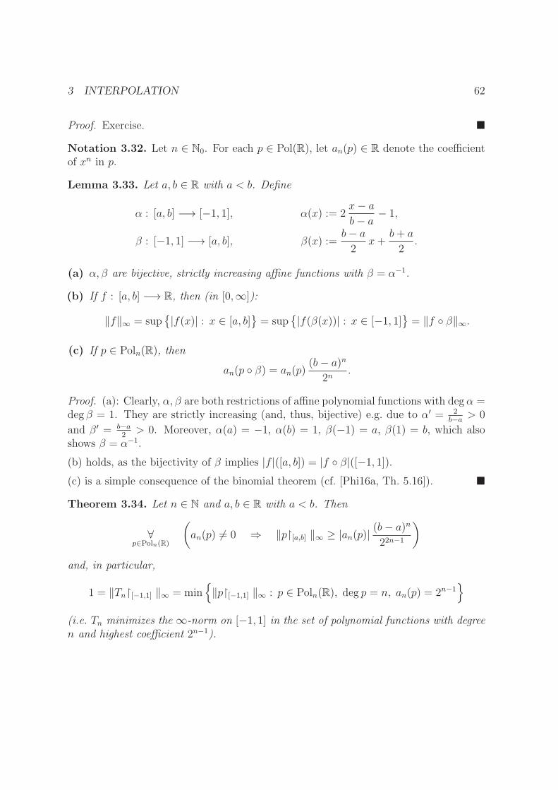
3 INTERPOLATION 62
Proof. Exercise. �
Notation 3.32. Let n ∈ N0. For each p ∈ Pol(R), let an(p) ∈ R denote the coefficientof xn in p.
Lemma 3.33. Let a, b ∈ R with a < b. Define
α : [a, b] −→ [−1, 1], α(x) := 2x− ab− a − 1,
β : [−1, 1] −→ [a, b], β(x) :=b− a2
x+b+ a
2.
(a) α, β are bijective, strictly increasing affine functions with β = α−1.
(b) If f : [a, b] −→ R, then (in [0,∞]):
‖f‖∞ = sup{|f(x)| : x ∈ [a, b]
}= sup
{|f(β(x))| : x ∈ [−1, 1]
}= ‖f ◦ β‖∞.
(c) If p ∈ Poln(R), then
an(p ◦ β) = an(p)(b− a)n
2n.
Proof. (a): Clearly, α, β are both restrictions of affine polynomial functions with degα =deg β = 1. They are strictly increasing (and, thus, bijective) e.g. due to α′ = 2
b−a> 0
and β′ = b−a2> 0. Moreover, α(a) = −1, α(b) = 1, β(−1) = a, β(1) = b, which also
shows β = α−1.
(b) holds, as the bijectivity of β implies |f |([a, b]) = |f ◦ β|([−1, 1]).(c) is a simple consequence of the binomial theorem (cf. [Phi16a, Th. 5.16]). �
Theorem 3.34. Let n ∈ N and a, b ∈ R with a < b. Then
∀p∈Poln(R)
(an(p) 6= 0 ⇒ ‖p↾[a,b] ‖∞ ≥ |an(p)|
(b− a)n22n−1
)
and, in particular,
1 = ‖Tn↾[−1,1] ‖∞ = min{‖p↾[−1,1] ‖∞ : p ∈ Poln(R), deg p = n, an(p) = 2n−1
}
(i.e. Tn minimizes the ∞-norm on [−1, 1] in the set of polynomial functions with degreen and highest coefficient 2n−1).

3 INTERPOLATION 63
Proof. We first consider the special case a = −1, b = 1, and an(p) = 2n−1. Seeking acontradiction, assume p ∈ Poln(R) with deg p = n, an(p) = 2n−1, and ‖p↾[−1,1] ‖∞ < 1.Using Th. 3.31(g), we obtain
∀k∈{0,...,n}
(p− Tn)(cos
kπ
n
){< 0 for k even,
> 0 for k odd,
showing p − Tn to have at least n zeros due to the intermediate value theorem (cf.[Phi16a, Th. 7.57]). Since p, Tn ∈ Poln(R) with an(p) = an(Tn) = 2n−1, we havep− Tn ∈ Poln−1(R) and the n zeros yield p− Tn = 0 in contradiction to p 6= Tn. Thus,there must exist x0 ∈ [−1, 1] such that |p(x0)| ≥ 1. Now if q ∈ Poln(R) is arbitrary withan(q) 6= 0 and p := 2n−1
an(q)q, then p ∈ Poln(R) with an(p) = 2n−1 and, due to the special
case,
∃x0∈[−1,1]
|q(x0)| =∣∣∣∣an(q)
2n−1p(x0)
∣∣∣∣ ≥|an(q)|2n−1
,
as desired. Moreover, on the interval [a, b], one then obtains
‖q↾[a,b] ‖∞Lem. 3.33(b)
= ‖q ◦ β‖∞Lem. 3.33(c)
≥ |an(q)|(b− a)n22n−1
,
thereby completing the proof. �
Example 3.35. Let n ∈ N and a, b ∈ R with a < b. As mentioned in Rem. 3.28,minimizing the error in (3.33) leads to the problem of finding x0, . . . , xn ∈ [a, b] suchthat
max
{n∏
j=0
|x− xj| : x ∈ [a, b]
}
is minimized. In other words, one needs to find the zeros of a monic polynomial functionp in Poln+1(R) such that p minimizes the ∞-norm on [a, b]. According to Th. 3.34, fora = −1, b = 1, p = Tn+1/2
n, which, according to Th. 3.31(f) has zeros
xj = cos
(2(j + 1)− 1
2(n+ 1)π
)= cos
(2j + 1
2n+ 2π
), j ∈ {0, . . . , n}.
In the general case, we then obtain the solution p by using the functions α, β of Lem.3.33: According to Lem. 3.33(b), we have p ◦ β = cTn+1, where c ∈ R is chosen suchthat an+1(p) = 1. By Lem. 3.33(c),
c · 2n = an+1(p ◦ β) = an+1(p)(b− a)n+1
2n+1=
(b− a)n+1
2n+1⇒ c =
(b− a)n+1
22n+1,
implying p = (Tn+1 ◦ α) · (b−a)n+1
22n+1 with the zeros
xj = β
(cos
(2j + 1
2n+ 2π
)), j ∈ {0, . . . , n}.

3 INTERPOLATION 64
Theorem 3.36. Let n ∈ N and a, b ∈ R with a < b. Assume s ∈ R \ [a, b] and define
cs :=1
Tn(α(s))∈ R \ {0}, ps := cs (Tn ◦ α) ∈ Poln(R),
where α : [a, b] −→ [−1, 1] is as in Lem. 3.33, extended to α : R −→ R (also noteα(s) /∈ [−1, 1] and Tn(α(s)) 6= 0). Then
|cs| = ‖ps↾[a,b] ‖∞ = min{‖p↾[a,b] ‖∞ : p ∈ Poln(R), deg p = n, p(s) = 1
}
(i.e. ps minimizes the ∞-norm on [a, b] in the set of polynomial functions with degree nand value 1 at s).
Proof. Exercise. �
3.3 Spline Interpolation
3.3.1 Introduction, Definition of Splines
In the previous sections, we have used a single polynomial to interpolate given datapoints. If the number of data points is large, then the degree of the interpolatingpolynomial is likewise large. If the data points are given by a function, and the goalis for the interpolating polynomial to approximate that function, then, in general, onemight need many data points to achieve a desired accuracy. We have also seen that theinterpolating polynomials tend to be large in the vicinity of the outermost data points,where strong oscillations are typical. One possibility to counteract that behavior isto choose an additional number of data points in the vicinity of the boundary of theconsidered interval (cf. Rem. 3.28).
The advantage of the approach of the previous sections is that the interpolating poly-nomial is C∞ (i.e. it has derivatives of all orders) and one can make sure (by Hermiteinterpolation) that, in a given point x0, the derivatives of the interpolating polynomial pagree with the derivatives of a given function in x0 (which, again, will typically increasethe degree of p). The disadvantage is that one often needs interpolating polynomials oflarge degrees, which can be difficult to handle (e.g. numerical problems resulting fromlarge numbers occurring during calculations).
Spline interpolation follows a different approach: Instead of using one single interpo-lating polynomial of potentially large degree, one uses a piecewise interpolation, fittingtogether polynomials of low degree (e.g. 1 or 3). The resulting function s will typicallynot be of class C∞, but merely of class C or C2, and the derivatives of s will usually not

3 INTERPOLATION 65
agree with the derivatives of a given f (only the values of f and s will agree in the datapoints). The advantage is that one only needs to deal with polynomials of low degree. Ifone does not need high differentiability of the interpolating function and one is mostlyinterested in a good approximation with respect to ‖ · ‖∞, then spline interpolation isusually a good option.
Definition 3.37. Let a, b ∈ R, a < b. Then, given N ∈ N,
∆ := (x0, . . . , xN) ∈ RN+1 (3.39)
is called a knot vector for [a, b] if, and only if, it corresponds to a partition a = x0 <x1 < · · · < xN = b of [a, b]. The xk are then also called knots. Let l ∈ N. A spline oforder l for ∆ is a function s ∈ C l−1[a, b] such that, for each k ∈ {0, . . . , N − 1}, thereexists a polynomial function pk ∈ Poll(R) that coincides with s on [xk, xk+1]. The set ofall such splines is denoted by S∆,l:
S∆,l :=
{s ∈ C l−1[a, b] : ∀
k∈{0,...,N−1}∃
pk∈Poll(R)pk↾[xk,xk+1]= s↾[xk,xk+1]
}. (3.40)
Of particular importance are the elements of S∆,1 (linear splines) and of S∆,3 (cubicsplines). It is also useful to define
S∆,0 := span{χk : k ∈ {0, . . . , N − 1}
}, (3.41)
where
∀k∈{0,...,N−1}
χk : [a, b] −→ R, χk(x) :=
{1 if x ∈ [xk, xk+1[,
0 if x /∈ [xk, xk+1[,
i.e. each χk is a step function, namely the characteristic function of the interval [xk, xk+1[.We call the elements of S∆,0 splines of order 0.
Remark and Definition 3.38. In the situation of Def. 3.37, let k ∈ {0, . . . , N − 1}.If s ∈ S∆,l, l ∈ N0, then, as s↾]xk,xk+1[ coincides with a polynomial function of degree atmost l, on ]xk, xk+1[ the derivative s(l) exists and is constant, i.e. there exists αk ∈ R
such that s(l)↾]xk,xk+1[≡ αk. We extend s(l) to all of [a, b] by defining
s(l) :=N−1∑
k=0
αk χk ∈ S∆,0. (3.42)
Definition 3.39. In the situation of Def. 3.37, if s ∈ S∆,0, then, for each l ∈ N0, definethe lth antiderivative Il(s) : [a, b] −→ R of s recursively by letting
I0(s) := s, ∀l∈N0
Il+1(s)(x) :=
∫ x
a
Il(s)(t) dt .
3 INTERPOLATION 66
Theorem 3.40. Let a, b ∈ R, a < b, N ∈ N, l ∈ N0, with ∆ := (x0, . . . , xN ) being aknot vector for [a, b]. Then the following statements hold true:
(a) Poll(R) ⊆ S∆,l (here, and in the following, we are sometimes a bit lax regarding thenotation, implicitly identifying polynomials on R with their respective restriction on[a, b]).
(b) For each j ∈ {0, . . . , l}, we have
s ∈ S∆,l ⇒ s(j) ∈ S∆,l−j.
(c) If s ∈ S∆,0 and S := Il(s) is the lth antiderivative of s as defined in Def. 3.39, thenS ∈ S∆,l.
(d) S∆,l is an (N+ l)-dimensional vector space over R and, if, for each k ∈ {0, . . . , N−1}, Xk := Il(χk) is the lth antiderivative of χk, then
B :={Xk : k ∈ {0, . . . , N − 1}
}∪{xj : j ∈ {0, . . . , l − 1}
}
forms a basis of S∆,l.
Proof. (a) is clear from the definition of S∆,l.
(b): For j ∈ {0, . . . , l − 1}, (b) holds since s ∈ C l−1[a, b] implies s(j) ∈ C l−j−1[a, b] and
pk ∈ Poll(R) implies p(j)k ∈ Poll−j(R). For j = l, (b) holds due to Rem. and Def. 3.38.
(c): We obtain the continuity of I1(s) from Th. C.6 of the appendix. We then apply thefundamental theorem of calculus (cf. [Phi16a, Th. 10.20(a)]) (l − 1) times to I1(s) toobtain S ∈ C l−1[a, b]. For each k ∈ {0, . . . , N − 1}, we apply the fundamental theoremof calculus l times on [xk, xk+1] to obtain S↾[xk,xk+1]∈ Poll(R).
(d): S∆,l being a vector space over R is a consequence of both C l−1[a, b] and Poll(R)being vector spaces over R. Since B ⊆ S∆,l by (a),(c) and, clearly, #B = N + l, itmerely remains to show that B is, indeed, a basis of S∆,l. Let s ∈ S∆,l. Since s
(l) ∈ S∆,0,
there exist α0, . . . , αN−1 ∈ R such that s(l) =∑N−1
k=0 αkχk. If s :=∑N−1
k=0 αkXk, thens(l) = s(l). We need to show (s − s) ∈ Poll−1(R). To this end, let k ∈ {1, . . . , N − 1}.Then the fundamental theorem of calculus yields p := (s − s)↾[xk−1,xk]∈ Poll−1(R) andq := (s− s)↾[xk,xk+1]∈ Poll−1(R). However, as s− s is C l−1, we also know
∀j∈{0,...,l−1}
p(j)(xk) = q(j)(xk),
implying p = q due to Th. 3.10(b) about Hermite interpolation. As k ∈ {1, . . . , N − 1}was arbitrary, this shows (s − s) ∈ Poll−1(R) and spanB = S∆,l. It remains to show

3 INTERPOLATION 67
that B is linearly independent. To this end assume
∃p∈Poll−1(R)
∃α0,...,αN−1∈R
∀x∈[a,b]
p(x) +N−1∑
k=0
αkXk(x) = 0.
Taking the derivative l times then yields
∀x∈[a,b]
N−1∑
k=0
αkχk(x) = 0.
As the χk are clearly linearly independent, we obtain α0 = · · · = αN−1 = 0, implyingp = 0 as well. Thus, B is linearly independent and, hence, a basis of S∆,l. �
3.3.2 Linear Splines
Given a node vector as in (3.39), and values y0, . . . , yN ∈ R, a corresponding linearspline is a continuous, piecewise linear function s satisfying s(xk) = yk. In this case,existence, uniqueness, and an error estimate are still rather simple to obtain:
Theorem 3.41. Let a, b ∈ R, a < b. Then, given N ∈ N, a knot vector ∆ :=(x0, . . . , xN ) ∈ RN+1 for [a, b], and values (y0, . . . , yN ) ∈ RN+1, there exists a uniqueinterpolating linear spline s ∈ S∆,1 satisfying
s(xk) = yk for each k ∈ {0, . . . , N}. (3.43)
Moreover, s is explicitly given by
s(x) = yk +yk+1 − ykxk+1 − xk
(x− xk) for each x ∈ [xk, xk+1]. (3.44)
If f ∈ C2[a, b] and yk = f(xk), then the following error estimate holds:
‖f − s‖∞ ≤1
8‖f ′′‖∞ h2, (3.45)
whereh := h(∆) := max
{xk+1 − xk : k ∈ {0, . . . , N − 1}
}
is the mesh size of the partition ∆.
Proof. Since s defined by (3.44) clearly satisfies (3.43), is continuous on [a, b], and,for each k ∈ {0, . . . , N}, the definition of (3.44) extends to a unique polynomial inPol1(R), we already have existence. Uniqueness is equally obvious, since, for each k, the

3 INTERPOLATION 68
prescribed values in xk and xk+1 uniquely determine a polynomial in Pol1(R) and, thus,s. For the error estimate, consider x ∈ [xk, xk+1], k ∈ {0, . . . , N − 1}. Note that, due tothe inequality αβ ≤
(α+β2
)2valid for all α, β ∈ R, one has
(x− xk)(xk+1 − x) ≤((x− xk) + (xk+1 − x)
2
)2
≤ h2
4. (3.46)
Moreover, on [xk, xk+1], s coincides with the interpolating polynomial p ∈ Pol1(R) withp(xk) = f(xk) and p(xk+1) = f(xk+1). Thus, we can use (3.31) to compute
∣∣f(x)− s(x)∣∣ =
∣∣f(x)− p(x)∣∣ ≤ ‖f
′′‖∞2!
(x− xk)(xk+1 − x)(3.46)
≤ 1
8‖f ′′‖∞ h2,
thereby proving (3.45). �
3.3.3 Cubic Splines
Given a knot vector
∆ = (x0, . . . , xN) ∈ RN+1 and values (y0, . . . , yN) ∈ RN+1, (3.47)
the task is to find an interpolating cubic spline, i.e. an element s of S∆,3 satisfying
s(xk) = yk for each k ∈ {0, . . . , N}. (3.48)
As we require s ∈ S∆,3, according to (3.40), for each k ∈ {0, . . . , N − 1}, we must findpk ∈ Pol3(R) such that pk↾[xk,xk+1]= s↾[xk,xk+1]. To that end, for each k ∈ {0, . . . , N −1},we employ the ansatz
pk(x) = ak + bk(x− xk) + ck(x− xk)2 + dk(x− xk)3 (3.49a)
with suitable(ak, bk, ck, dk) ∈ R4; (3.49b)
to then define s bys(x) = pk(x) for each x ∈ [xk, xk+1]. (3.49c)
It is immediate that s is well-defined by (3.49c) and an element of S∆,3 (cf. (3.40))satisfying (3.48) if, and only if,
p0(x0) = y0, (3.50a)
pk−1(xk) = yk = pk(xk) for each k ∈ {1, . . . , N − 1}, (3.50b)
pN−1(xN) = yN , (3.50c)
p′k−1(xk) = p′k(xk) for each k ∈ {1, . . . , N − 1}, (3.50d)
p′′k−1(xk) = p′′k(xk) for each k ∈ {1, . . . , N − 1}, (3.50e)

3 INTERPOLATION 69
using the convention {1, . . . , N − 1} = ∅ for N − 1 < 1. Note that (3.50) constitutes asystem of 2 + 4(N − 1) = 4N − 2 conditions, while (3.49a) provides 4N variables. Thisalready indicates that one will be able to impose two additional conditions on s. Onetypically imposes so-called boundary conditions, i.e. conditions on the values for s or itsderivatives at x0 and xN (see (3.61) below for commonly used boundary conditions).
In order to show that one can, indeed, choose the ak, bk, ck, dk such that all conditions of(3.50) are satisfied, the strategy is to transform (3.50) into an equivalent linear system.An analysis of the structure of that system will then show that it has a solution. Thetrick that will lead to the linear system is the introduction of
s′′k := s′′(xk), k ∈ {0, . . . , N}, (3.51)
as new variables. As we will see in the following lemma, (3.50) is satisfied if, and onlyif, the s′′k satisfy the linear system (3.53):
Lemma 3.42. Given a knot vector and values according to (3.47), and introducing theabbreviations
hk := xk+1 − xk, for each k ∈ {0, . . . , N − 1}, (3.52a)
gk := 6
(yk+1 − yk
hk− yk − yk−1
hk−1︸ ︷︷ ︸(hk+hk−1)[xk−1,xk,xk+1]
)for each k ∈ {1, . . . , N − 1}, (3.52b)
the pk ∈ Pol3(R) of (3.49a) satisfy (3.50) (and that means s given by (3.49c) is in S∆,3
and satisfies (3.48)) if, and only if, the N +1 numbers s′′0, . . . , s′′N defined by (3.51) solve
the linear system consisting of the N − 1 equations
hks′′k + 2(hk + hk+1)s
′′k+1 + hk+1s
′′k+2 = gk+1, k ∈ {0, . . . , N − 2}, (3.53)
and the ak, bk, ck, dk are given in terms of the xk, yk and s′′k by
ak = yk for each k ∈ {0, . . . , N − 1}, (3.54a)
bk =yk+1 − yk
hk− hk
6(s′′k+1 + 2s′′k) for each k ∈ {0, . . . , N − 1}, (3.54b)
ck =s′′k2
for each k ∈ {0, . . . , N − 1}, (3.54c)
dk =s′′k+1 − s′′k
6hkfor each k ∈ {0, . . . , N − 1}. (3.54d)
Proof. First, for subsequent use, from (3.49a), we obtain the first two derivatives of thepk for each k ∈ {0, . . . , N − 1}:
p′k(x) = bk + 2ck(x− xk) + 3dk(x− xk)2, (3.55a)
p′′k(x) = 2ck + 6dk(x− xk). (3.55b)

3 INTERPOLATION 70
As usual, for the claimed equivalence, we prove two implications.
(3.50) implies (3.53) and (3.54):
Plugging x = xk into (3.49a) yields
pk(xk) = ak for each k ∈ {0, . . . , N − 1}. (3.56)
Thus, (3.54a) is a consequence of (3.50a) and (3.50b).
Plugging x = xk into (3.55b) yields
s′′k = p′′k(xk) = 2ck for each k ∈ {0, . . . , N − 1}, (3.57)
i.e. (3.54c).
Plugging (3.50e), i.e. p′′k−1(xk) = p′′k(xk), into (3.55b) yields
2ck−1 + 6dk−1(xk − xk−1) = 2ck for each k ∈ {1, . . . , N − 1}. (3.58a)
When using (3.54c) and solving for dk−1, one obtains
dk−1 =s′′k − s′′k−1
6hk−1
for each k ∈ {1, . . . , N − 1}, (3.58b)
i.e. the relation of (3.54d) for each k ∈ {0, . . . , N − 2}. Moreover, (3.51) and (3.55b)imply
s′′N = s′′(xN) = p′′N−1(xN) = 2cN−1 + 6dN−1hN−1, (3.58c)
which, after solving for dN−1, shows that the relation of (3.54d) also holds for k = N−1.Plugging the first part of (3.50b) and (3.50c), i.e. pk−1(xk) = yk into (3.49a) yields
ak−1 + bk−1 hk−1 + ck−1 h2k−1 + dk−1 h
3k−1 = yk for each k ∈ {1, . . . , N}. (3.59a)
When using (3.54a), (3.54c), (3.54d), and solving for bk−1, one obtains
bk−1 =yk − yk−1
hk−1
− s′′k−1 hk−1
2− s
′′k − s′′k−1
6hk−1
h2k−1 =yk − yk−1
hk−1
− hk−1
6(s′′k+2s′′k−1) (3.59b)
for each k ∈ {1, . . . , N}, i.e. (3.54b).Plugging (3.50d), i.e. p′k−1(xk) = p′k(xk), into (3.55a) yields
bk−1 + 2ck−1 hk−1 + 3dk−1 h2k−1 = bk for each k ∈ {1, . . . , N − 1}. (3.60a)
Finally, applying (3.54b), (3.54c), and (3.54d), one obtains
yk − yk−1
hk−1
− hk−1
6(s′′k+2s′′k−1)+s
′′k−1 hk−1+
s′′k − s′′k−1
2hk−1 =
yk+1 − ykhk
− hk6
(s′′k+1+2s′′k),
(3.60b)

3 INTERPOLATION 71
or, rearranged,
hk−1 s′′k−1 + 2(hk−1 + hk)s
′′k + hk s
′′k+1 = gk, k ∈ {1, . . . , N − 1}, (3.60c)
which is (3.53).
(3.53) and (3.54) imply (3.50):
First, note that plugging x = xk into (3.55b) again yields s′′k = p′′k(xk). Using (3.54a) in(3.49a) yields (3.50a) and the pk(xk) = yk part of (3.50b). Since (3.54b) is equivalent to(3.59b), and (3.59b) (when using (3.54a), (3.54c), and (3.54d)) implies (3.59a), which,in turn, is equivalent to pk−1(xk) = yk for each k ∈ {1, . . . , N}, we see that (3.54)implies (3.50c) and the pk−1(xk) = yk part of (3.50b). Since (3.53) is equivalent to(3.60c) and (3.60b), and (3.60b) (when using (3.54a) – (3.54d)) implies (3.60a), which,in turn, is equivalent to p′k−1(xk) = p′k(xk) for each k ∈ {1, . . . , N − 1}, we see that(3.53) and (3.54) implies (3.50d). Finally, (3.54d) is equivalent to (3.58b), which (whenusing (3.54c)) implies (3.58a). Since (3.58a) is equivalent to p′′k−1(xk) = p′′k(xk) for eachk ∈ {1, . . . , N − 1}, (3.54) also implies (3.50d), concluding the proof of the lemma. �
As already mentioned after formulating (3.50), (3.50) yields two conditions less thanthere are variables. Not surprisingly, the same is true in the linear system (3.53), wherethere are N − 1 equations for N + 1 variables. As also mentioned before, this allows toimpose two additional conditions. Here are some of the most commonly used additionalconditions:
Natural boundary conditions:
s′′(x0) = s′′(xN) = 0. (3.61a)
Periodic boundary conditions:
s′(x0) = s′(xN) and s′′(x0) = s′′(xN). (3.61b)
Dirichlet boundary conditions for the first derivative:
s′(x0) = y′0 ∈ R and s′(xN) = y′N ∈ R. (3.61c)
Due to time constraints, we will only investigate the most simple of these cases, namelynatural boundary conditions, in the following.
Since (3.61a) fixes the values of s′′0 and s′′N as 0, (3.53) now yields a linear systemconsisting of N − 1 equations for the N − 1 variables s′′1 through s′′N−1. We can rewritethis system in matrix form
As′′ = g (3.62a)

3 INTERPOLATION 72
by introducing the matrix
A :=
2(h0 + h1) h1h1 2(h1 + h2) h2
h2 2(h2 + h3) h3. . .
. . .. . .
. . .. . .
. . .
hN−3 2(hN−3 + hN−2) hN−2
hN−2 2(hN−2 + hN−1)
(3.62b)
and the vectors
s′′ :=
s′′1...
s′′N−1
, g :=
g1...
gN−1
. (3.62c)
The matrix A from (3.62b) belongs to an especially benign class of matrices, so-calledstrictly diagonally dominant matrices:
Definition 3.43. Let A ∈ M(N,C), N ∈ N. Then A is called strictly diagonallydominant if, and only if,
N∑
j=1j 6=k
|akj| < |akk| for each k ∈ {1, . . . , N}. (3.63)
Lemma 3.44. Let A ∈ M(N,K), N ∈ N. If A is strictly diagonally dominant, then,for each x ∈ KN ,
‖x‖∞ ≤ max
1
|akk| −∑N
j=1j 6=k|akj|
: k ∈ {1, . . . , N}
‖Ax‖∞. (3.64)
In particular, A is invertible with
‖A−1‖∞ ≤ max
1
|akk| −∑N
j=1j 6=k|akj|
: k ∈ {1, . . . , N}
, (3.65)
where ‖A−1‖∞ denotes the row sum norm according to Ex. 2.18(a).
Proof. Exercise. �
3 INTERPOLATION 73
Theorem 3.45. Given a knot vector and values according to (3.47), there is a uniquecubic spline s ∈ S∆,3 that satisfies (3.48) and the natural boundary conditions (3.61a).Moreover, s can be computed by first solving the linear system (3.62) for the s′′k (the hkand the gk are given by (3.52)), then determining the ak, bk, ck, and dk according to(3.54), and, finally, using (3.49) to get s.
Proof. Lemma 3.42 shows that the existence and uniqueness of s is equivalent to (3.62a)having a unique solution. That (3.62a) does, indeed, have a unique solution follows fromLem. 3.44, as A as defined in (3.62b) is clearly strictly diagonally dominant. It is alsopart of the statement of Lem. 3.42 that s can be computed in the described way. �
Theorem 3.46. Let a, b ∈ R, a < b, and f ∈ C4[a, b]. Moreover, given N ∈ N and aknot vector ∆ := (x0, . . . , xN) ∈ RN+1 for [a, b], define
hk := xk+1 − xk for each k ∈ {0, . . . , N − 1}, (3.66a)
hmin := min{hk : k ∈ {0, . . . , N − 1}
}, (3.66b)
hmax := max{hk : k ∈ {0, . . . , N − 1}
}. (3.66c)
Let s ∈ S∆,3 be any cubic spline function satisfying s(xk) = f(xk) for each k ∈{0, . . . , N}. If there exists C > 0 such that
max{∣∣s′′(xk)− f ′′(xk)
∣∣ : k ∈ {0, . . . , N}}≤ C ‖f (4)‖∞ h2max, (3.67)
then the following error estimates hold:
‖f − s‖∞ ≤ c ‖f (4)‖∞ h4max, (3.68a)
‖f ′ − s′‖∞ ≤ 2c ‖f (4)‖∞ h3max, (3.68b)
‖f ′′ − s′′‖∞ ≤ 2c ‖f (4)‖∞ h2max, (3.68c)
‖f ′′′ − s′′′‖∞ ≤ 2c ‖f (4)‖∞ h1max, (3.68d)
where
c :=hmax
hmin
(C +
1
4
). (3.69)
At the xk, the third derivative s′′′ does not need to exist. In that case, (3.68d) is to beinterpreted to mean that the estimate holds for all values of one-sided third derivativesof s (which must exist, since s agrees with a polynomial on each [xk, xk+1]).
Proof. Exercise. �
3 INTERPOLATION 74
Theorem 3.47. Once again, consider the situation of Th. 3.46, but, instead of (3.67),assume that the interpolating cubic spline s satisfies natural boundary conditions s′′(a) =s′′(b) = 0. If f ∈ C4[a, b] satisfies f ′′(a) = f ′′(b) = 0, then it follows that s satisfies(3.67) with C = 3/4, and, in consequence, the error estimates (3.68) with c = hmax/hmin.
Proof. We merely need to show that (3.67) holds with C = 3/4. Since s is the interpo-lating cubic spline satisfying natural boundary conditions, s′′ satisfies the linear system(3.62a). Deviding, for each k ∈ {1, . . . , N − 1}, the (k − 1)th equation of that systemby 3(hk−1 + hk) yields the form
Bs′′ = g, (3.70a)
with
B :=
23
h13(h0+h1)
h13(h1+h2)
23
h23(h1+h2)
h23(h2+h3)
23
h33(h2+h3)
. . .. . .
. . .. . .
. . .. . .
hN−3
3(hN−3+hN−2)23
hN−2
3(hN−3+hN−2)
hN−2
3(hN−2+hN−1)23
(3.70b)
and
g :=
g1...
gN−1
:=
g13(h0+h1)
...gN−1
3(hN−2+hN−1)
. (3.70c)
Taylor’s theorem applied to f ′′ provides, for each k ∈ {1, . . . , N − 1}, αk ∈]xk−1, xk[and βk ∈]xk, xk+1[ such that the following equations (3.71) hold, where (3.71a) has been
multiplied by hk−1
3(hk−1+hk)and (3.71b) has been multiplied by hk
3(hk−1+hk):
hk−1 f′′(xk−1)
3(hk−1 + hk)=
hk−1 f′′(xk)
3(hk−1 + hk)− h2k−1 f
′′′(xk)
3(hk−1 + hk)+h3k−1f
(4)(αk)
6(hk−1 + hk), (3.71a)
hk f′′(xk+1)
3(hk−1 + hk)=
hk f′′(xk)
3(hk−1 + hk)+
h2k f′′′(xk)
3(hk−1 + hk)+
h3kf(4)(βk)
6(hk−1 + hk). (3.71b)
Adding (3.71a) and (3.71b) results in
hk−1
3(hk−1 + hk)f ′′(xk−1) +
2
3f ′′(xk) +
hk3(hk−1 + hk)
f ′′(xk+1) = f ′′(xk) +Rk + δk, (3.72a)

3 INTERPOLATION 75
where
Rk :=1
3(hk − hk−1) f
′′′(xk), (3.72b)
δk :=1
6(hk−1 + hk)
(h3k−1f
(4)(αk) + h3kf(4)(βk)
). (3.72c)
Using the matrix B from (3.70b), (3.72a) takes the form
B
f ′′(x1)...
f ′′(xN−1)
=
f ′′(x1)...
f ′′(xN−1)
+
R1...
RN−1
+
δ1...
δN−1
. (3.73)
In the same way we applied Taylor’s theorem to f ′′ to obtain (3.71), we now applyTaylor’s theorem to f to obtain for each k ∈ {1, . . . , N − 1}, ξk ∈]xk, xk+1[ and ηk ∈]xk−1, xk[ such that
f(xk+1) = f(xk) + hk f′(xk) +
h2k2f ′′(xk) +
h3k6f ′′′(xk) +
h4k24f (4)(ξk), (3.74a)
f(xk−1) = f(xk)− hk−1 f′(xk) +
h2k−1
2f ′′(xk)−
h3k−1
6f ′′′(xk) +
h4k−1
24f (4)(ηk). (3.74b)
Multiplying (3.74a) and (3.74b) by 2/hk and 2/hk−1, respectively, leads to
2f(xk+1)− f(xk)
hk= 2 f ′(xk) + hk f
′′(xk) +h2k3f ′′′(xk) +
h3k12f (4)(ξk), (3.75a)
−2 f(xk)− f(xk−1)
hk−1
= −2 f ′(xk) + hk−1 f′′(xk)−
h2k−1
3f ′′′(xk) +
h3k−1
12f (4)(ηk). (3.75b)
Adding (3.75a) and (3.75b) followed by a division by hk−1 + hk yields
2f(xk+1)− f(xk)hk(hk−1 + hk)
− 2f(xk)− f(xk−1)
hk−1(hk−1 + hk)= f ′′(xk) +Rk + δk, (3.76)
where Rk is as in (3.72b) and
δk :=1
12(hk−1 + hk)
(h3k−1f
(4)(ηk) + h3kf(4)(ξk)
).
Observing that
gk(3.70c)=
gk3(hk−1 + hk)
(3.52b), yk=f(xk)= 2
f(xk+1)− f(xk)hk(hk−1 + hk)
− 2f(xk)− f(xk−1)
hk−1(hk−1 + hk),
3 INTERPOLATION 76
we can write (3.76) as
f ′′(x1)...
f ′′(xN−1)
=
g1...
gN−1
−
R1...
RN−1
−
δ1...
δN−1
. (3.77)
Using (3.77) in the right-hand side of (3.73) and then subtracting (3.70a) from the resultyields
B
f ′′(x1)− s′′(x1)...
f ′′(xN−1)− s′′(xN−1)
=
δ1 − δ1...
δN−1 − δN−1
.
From2
3− hk−1
3(hk−1 + hk)− hk
3(hk−1 + hk)=
1
3for k ∈ {1, . . . , N − 1},
we conclude that B is strictly diagonally dominant, such that Lem. 3.44 allows us toestimate
max{∣∣f ′′(xk)− s′′(xk)
∣∣ : k ∈ {0, . . . , N}}≤ 3max
{|δk|+ |δk| : k ∈ {1, . . . , N − 1}
}
(∗)≤ 3
4h2max ‖f (4)‖∞, (3.78)
where
|δk|+ |δk| ≤(1
6+
1
12
)h3k−1 + h3khk−1 + hk
‖f (4)‖∞ ≤1
4h2max ‖f (4)‖∞
was used for the inequality at (∗). The estimate (3.78) shows that s satisfies (3.67) withC = 3/4, thereby concluding the proof of the theorem. �
Note that (3.68) is, in more than one way, much better than (3.45): From (3.68) weget convergence of the first three derivatives, and the convergence of ‖f − s‖∞ is alsomuch faster in (3.68) (proportional to h4 rather than to h2 in (3.45)). The disadvantageof (3.68), however, is that we needed to assume the existence of a continuous fourthderivative of f .
Remark 3.48. A piecewise interpolation by cubic polynomials different from splineinterpolation is given by carrying out a Hermite interpolation on each interval [xk, xk+1]such that the resulting function satisfies f(xk) = s(xk) as well as
f ′(xk) = s′(xk). (3.79)
The result will usually not be a spline, since s will usually not have second derivativesin the xk. On the other hand the corresponding cubic spline will usually not satisfy

3 INTERPOLATION 77
(3.79). Thus, one will prefer one or the other form of interpolation, depending on either(3.79) (i.e. the agreement of the first derivatives of the given and interpolating function)or s ∈ C2 being more important in the case at hand.
—
We conclude the section by depicting different interpolations of the functions f(x) =1/(x2 + 1) and f(x) = cos x on the interval [−6, 6] in Figures 3.1 and 3.2, respectively.While f is depicted as a solid blue curve, the interpolating polynomial of degree 6 isshown as a dotted black curve, the interpolating linear spline as a solid red curve, andthe interpolating cubic spline is shown as a dashed green curve. One clearly observes thelarge values and strong oscillations of the interpolating polynomial toward the bound-aries of the interval.
−6 −4 −2 0 2 4 6−0.2
0
0.2
0.4
0.6
0.8
1
1.2
f
linear spline
cubic spline
pol of deg 6
Figure 3.1: Different interpolations of f(x) = 1/(x2+1) with data points at (x0, . . . , x6)= (−6,−4, . . . , 4, 6).

4 NUMERICAL INTEGRATION 78
−6 −4 −2 0 2 4 6−1.5
−1
−0.5
0
0.5
1
1.5
f
linear spline
cubic spline
pol of deg 6
Figure 3.2: Different interpolations of f(x) = cos(x) with data points at (x0, . . . , x6) =(−6,−4, . . . , 4, 6).
4 Numerical Integration
4.1 Introduction
The goal is the computation of (an approximation of) the value of definite integrals
∫ b
a
f(x) dx . (4.1)
Even if we know from the fundamental theorem of calculus that f has an antiderivative,even for simple f , the antiderivative can often not be expressed in terms of so-calledelementary functions (such as polynomials, exponential functions, and trigonometricfunctions). An example is the important function
Φ(y) :=
∫ y
0
1√2π
e−x2
2 dx , (4.2)
4 NUMERICAL INTEGRATION 79
which can not be expressed by elementary functions.
On the other hand, as we will see, there are effective and efficient methods to computeaccurate approximations of such integrals. As a general rule, one can say that numericalintegration is easy, whereas symbolic integration is hard (for differentiation, one has thereverse situation – symbolic differentiation is easy, while numeric differentiation is hard).
A first approximative method for the evaluation of integrals is given by the very defini-tion of the Riemann integral. We recall it in the form of the following Th. 4.3. First,let us formally introduce some notation that, in part, we already used when studyingspline interpolation:
Notation 4.1. Given a real interval [a, b], a < b, (x0, . . . , xn) ∈ Rn+1, n ∈ N, is calleda partition of [a, b] if, and only if, a = x0 < x1 < · · · < xn = b (what was called a knotvector in the context of spline interpolation). A tagged partition of [a, b] is a partitiontogether with a vector (t1, . . . , tn) ∈ Rn such that ti ∈ [xi−1, xi] for each i ∈ {1, . . . , n}.Given a partition ∆ (with or without tags) of [a, b] as above, the number
h(∆) := max{hi : i ∈ {1, . . . , n}
}, hi := xi − xi−1, (4.3)
is called the mesh size of ∆. Moreover, if f : [a, b] −→ R, then
n∑
i=1
f(ti)hi (4.4)
is called the Riemann sum of f associated with a tagged partition of [a, b].
Notation 4.2. Given a real interval [a, b], a < b, we denote the set of all Riemannintegrable functions f : [a, b] −→ R by R[a, b].
Theorem 4.3. Given a real interval [a, b], a < b, a function f : [a, b] −→ R is in R[a, b]if, and only if, for each sequence of tagged partitions
∆k =((xk0, . . . , x
knk), (tk1, . . . , t
knk)), k ∈ N, (4.5)
of [a, b] such that limk→∞ h(∆k) = 0, the limit of associated Riemann sums
I(f) :=
∫ b
a
f(x) dx := limk→∞
nk∑
i=1
f(tki )hki (4.6)
exists. The limit is then unique and called the Riemann integral of f . Recall that everycontinuous and every piecewise continuous function on [a, b] is in R[a, b].
Proof. See, e.g., [Phi16a, Th. 10.10(d)]. �
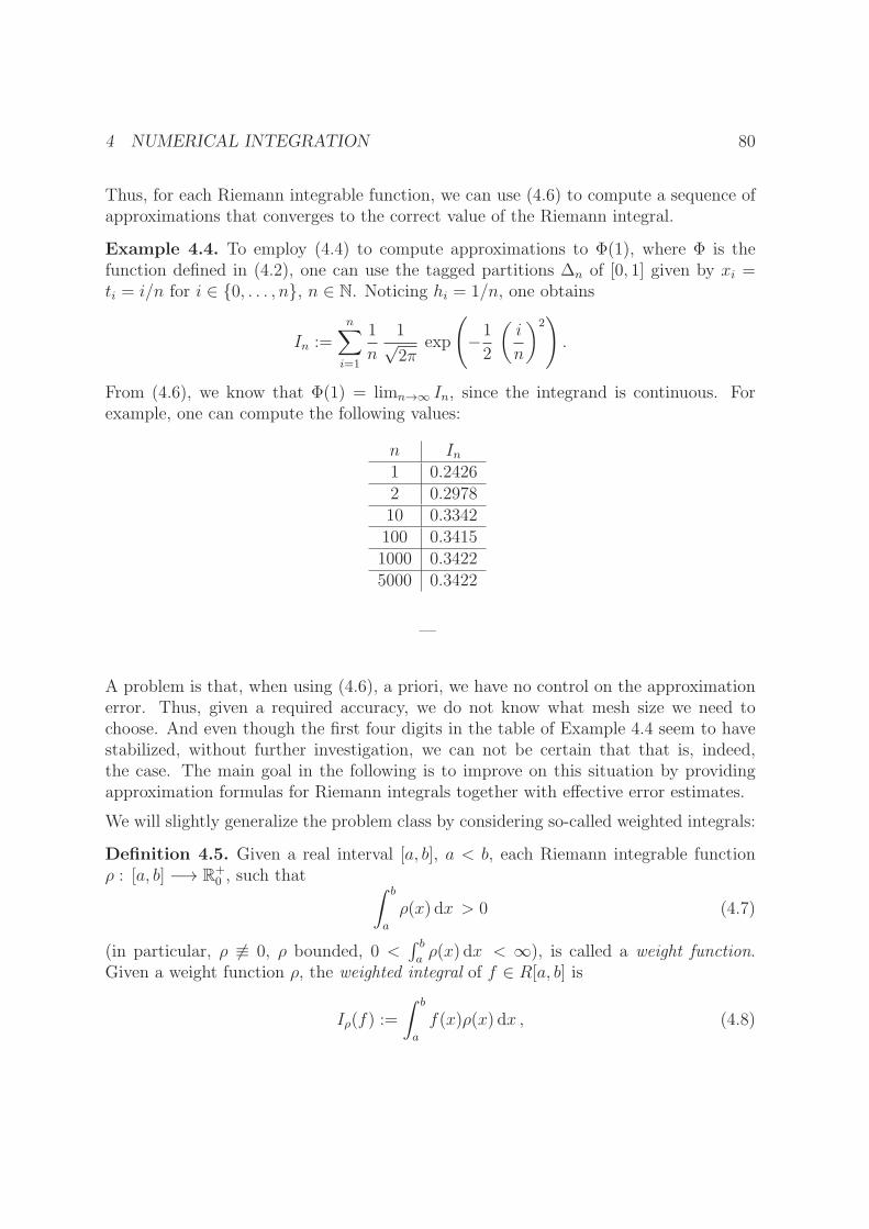
4 NUMERICAL INTEGRATION 80
Thus, for each Riemann integrable function, we can use (4.6) to compute a sequence ofapproximations that converges to the correct value of the Riemann integral.
Example 4.4. To employ (4.4) to compute approximations to Φ(1), where Φ is thefunction defined in (4.2), one can use the tagged partitions ∆n of [0, 1] given by xi =ti = i/n for i ∈ {0, . . . , n}, n ∈ N. Noticing hi = 1/n, one obtains
In :=n∑
i=1
1
n
1√2π
exp
(−1
2
(i
n
)2).
From (4.6), we know that Φ(1) = limn→∞ In, since the integrand is continuous. Forexample, one can compute the following values:
n In1 0.24262 0.297810 0.3342100 0.34151000 0.34225000 0.3422
—
A problem is that, when using (4.6), a priori, we have no control on the approximationerror. Thus, given a required accuracy, we do not know what mesh size we need tochoose. And even though the first four digits in the table of Example 4.4 seem to havestabilized, without further investigation, we can not be certain that that is, indeed,the case. The main goal in the following is to improve on this situation by providingapproximation formulas for Riemann integrals together with effective error estimates.
We will slightly generalize the problem class by considering so-called weighted integrals:
Definition 4.5. Given a real interval [a, b], a < b, each Riemann integrable functionρ : [a, b] −→ R+
0 , such that ∫ b
a
ρ(x) dx > 0 (4.7)
(in particular, ρ 6≡ 0, ρ bounded, 0 <∫ b
aρ(x) dx < ∞), is called a weight function.
Given a weight function ρ, the weighted integral of f ∈ R[a, b] is
Iρ(f) :=
∫ b
a
f(x)ρ(x) dx , (4.8)

4 NUMERICAL INTEGRATION 81
that means the usual integral I(f) corresponds to ρ ≡ 1 (note that fρ ∈ R[a, b], cf.[Phi16a, Th. 10.18(d)]).
—
In the sequel, we will first study methods designed for the numerical solution of non-weighted integrals (i.e. ρ ≡ 1) in Sections 4.2, 4.3, and 4.5, followed by an investigationof Gaussian quadrature in Sec. 4.6, which is suitable for the numerical solution of bothweighted and nonweighted integrals.
Definition 4.6. Given a real interval [a, b], a < b, in a generalization of the Riemannsums (4.4), a map
In : R[a, b] −→ R, In(f) = (b− a)n∑
i=0
σi f(xi), (4.9)
is called a quadrature formula or a quadrature rule with distinct points x0, . . . , xn ∈ [a, b]and weights σ0, . . . , σn ∈ R, n ∈ N0.
Remark 4.7. Note that every quadrature rule constitutes a linear functional on R[a, b].
—
A decent quadrature rule should give the exact integral for polynomials of low degree.This gives rise to the next definition:
Definition 4.8. Given a real interval [a, b], a < b, and a weight function ρ : [a, b] −→R+
0 , a quadrature rule In is defined to have the degree of accuracy r ∈ N0 if, and onlyif,
In(xm) =
∫ b
a
xm ρ(x) dx for each m ∈ {0, . . . , r}, (4.10a)
but,
In(xr+1) 6=
∫ b
a
xr+1 ρ(x) dx . (4.10b)
Remark 4.9. (a) Due to the linearity of In, In has degree of accuracy at least r ∈ N0
if, and only if, In is exact for each p ∈ Polr(R).
(b) A quadrature rule In as given by (4.9) can never be exact for the polynomial
p : R −→ R, p(x) :=n∏
i=0
(x− xi)2, (4.11)

4 NUMERICAL INTEGRATION 82
since
In(p) = 0 6=∫ b
a
p(x)ρ(x) dx . (4.12)
In particular, In can have degree of accuracy at most r = 2n+ 1.
(c) In view of (b), a quadrature rule In as given by (4.9) has any degree of accuracy(i.e. at least degree of accuracy 0) if, and only if,
∫ b
a
ρ(x) dx = In(1) = (b− a)n∑
i=0
σi, (4.13)
which simplifies ton∑
i=0
σi = 1 for ρ ≡ 1. (4.14)
4.2 Quadrature Rules Based on Interpolating Polynomials
In this section, we consider ρ ≡ 1, that means only nonweighted integrals. We can makeuse of interpolating polynomials to produce an abundance of useful quadrature rules.
Definition 4.10. Given a real interval [a, b], a < b, the quadrature rule based oninterpolating polynomials for the distinct points x0, . . . , xn ∈ [a, b], n ∈ N0, is definedby
In : R[a, b] −→ R, In(f) :=
∫ b
a
pn(x) dx , (4.15)
where pn = pn(f) ∈ Poln(R) is the interpolating polynomial corresponding to the datapoints (x0, f(x0)), . . . , (xn, f(xn)).
Theorem 4.11. Let [a, b] be a real interval, a < b, and let In be the quadrature rulebased on interpolating polynomials for the distinct points x0, . . . , xn ∈ [a, b], n ∈ N0, asdefined in (4.15).
(a) In is, indeed, a quadrature rule in the sense of Def. 4.6, where the weights σi,i ∈ {0, . . . , n}, are given in terms of the Lagrange basis polynomials Li of (3.10) by
σi =1
b− a
∫ b
a
Li(x) dx =1
b− a
∫ b
a
n∏
k=0k 6=i
x− xkxi − xk
dx
(∗)=
∫ 1
0
n∏
k=0k 6=i
t− tkti − tk
dt , where ti :=xi − ab− a .
(4.16)
4 NUMERICAL INTEGRATION 83
(b) In has at least degree of accuracy n, i.e. it is exact for each q ∈ Poln(R).
(c) For each f ∈ Cn+1[a, b], one has the error estimate
∣∣∣∣∫ b
a
f(x) dx − In(f)∣∣∣∣ ≤‖f (n+1)‖∞(n+ 1)!
∫ b
a
|ωn+1(x)| dx , (4.17)
where ωn+1(x) =∏n
i=0(x− xi) is the Newton basis polynomial.
Proof. (a): If pn is as in (4.15), then, according to (3.10), for each x ∈ R,
pn(x) =n∑
i=0
f(xi)Li(x) =n∑
i=0
f(xi)n∏
k=0k 6=i
x− xkxi − xk
.
Comparing with (4.9) then yields (4.16), where the equality labeled (∗) is due to
x− xkxi − xk
=x−ab−a− xk−a
b−axi−ab−a− xk−a
b−a
and the change of variables x 7→ t := x−ab−a
.
(b): For q ∈ Poln(R), we have pn(q) = q such that In(q) =∫ b
aq(x) dx is clear from
(4.15).
(c) follows by using (4.15) in combination with (3.31). �
Remark 4.12. If f ∈ C∞[a, b] and there exist K ∈ R+0 and R < (b − a)−1 such that
(3.32) holds, i.e.‖f (n)‖∞ ≤ Kn!Rn for each n ∈ N,
then, for each sequence of distinct numbers (x0, x1, . . . ) in [a, b], the correspondingquadrature rules based on interpolating polynomials converge, i.e.
limn→∞
∣∣∣∣∫ b
a
f(x) dx − In(f)∣∣∣∣ = 0 :
Indeed, |∫ b
af(x) dx − In(f)| ≤
∫ b
a‖f − pn‖∞ dx = (b− a) ‖f − pn‖∞ and limn→∞ ‖f −
pn‖∞ = 0 according to (3.34).
—
In certain situations, (4.17) can be improved by determining the sign of the error term(see Prop. 4.13 below). This information will come in handy when proving subsequenterror estimates for special cases.

4 NUMERICAL INTEGRATION 84
Proposition 4.13. Let [a, b] be a real interval, a < b, and let In be the quadrature rulebased on interpolating polynomials for the distinct points x0, . . . , xn ∈ [a, b], n ∈ N0, asdefined in (4.15). If ωn+1(x) =
∏ni=0(x − xi) has only one sign on [a, b] (i.e. ωn+1 ≥ 0
or ωn+1 ≤ 0 on [a, b], see Rem. 4.14 below), then, for each f ∈ Cn+1[a, b], there existsτ ∈ [a, b] such that
∫ b
a
f(x) dx − In(f) =f (n+1)(τ)
(n+ 1)!
∫ b
a
ωn+1(x) dx . (4.18)
In particular, if f (n+1) has just one sign as well, then one can infer the sign of the errorterm (i.e. of the right-hand side of (4.18)).
Proof. From Th. 3.25, we know that, for each x ∈ [a, b], there exists ξ(x) ∈ [a, b] suchthat (cf. (3.31))
f(x) = pn(x) +f (n+1)
(ξ(x)
)
(n+ 1)!ωn+1(x), (4.19)
where, according to Th. 3.25(c), the function x 7→ f (n+1)(ξ(x)
)is continuous on [a, b].
Thus, integrating (4.19) and applying the mean value theorem of integration (cf. [Phi17,(2.15f)]) yields τ ∈ [a, b] satisfying
∫ b
a
f(x) dx − In(f) =1
(n+ 1)!
∫ b
a
f (n+1)(ξ(x)
)ωn+1(x) dx =
f (n+1)(τ)
(n+ 1)!
∫ b
a
ωn+1(x) dx ,
proving (4.18). �
Remark 4.14. There exist precisely 3 examples where ωn+1 has only one sign on [a, b],namely ω1(x) = (x − a) ≥ 0, ω1(x) = (x − b) ≤ 0, and ω2(x) = (x − a)(x − b) ≤ 0. Inall other cases, there exists at least one xi ∈]a, b[. As xi is a simple zero of ωn+1, ωn+1
changes its sign in the interior of [a, b].
4.3 Newton-Cotes Formulas
We will now study quadrature rules based on interpolating polynomials with equally-spaced data points. In particular, we continue to assume ρ ≡ 1 (nonweighted integrals).
4.3.1 Definition, Weights, Degree of Accuracy
Definition and Remark 4.15. Given a real interval [a, b], a < b, a quadrature rulebased on interpolating polynomials according to Def. 4.10 is called a Newton-Cotes

4 NUMERICAL INTEGRATION 85
formula, also known as a Newton-Cotes quadrature rule if, and only if, the pointsx0, . . . , xn ∈ [a, b], n ∈ N, are equally-spaced. Moreover, a Newton-Cotes formula iscalled closed or a Newton-Cotes closed quadrature rule if, and only if,
xi := a+ i h, h :=b− an
, i ∈ {0, . . . , n}, n ∈ N. (4.20)
In the present context of equally-spaced xi, the discretization’s mesh size h is also calledstep size. It is an exercise to compute the weights of the Newton-Cotes closed quadraturerules. One obtains
σi = σi,n =1
n
∫ n
0
n∏
k=0k 6=i
s− ki− k ds . (4.21)
Given n, one can compute the σi explicitly and store or tabulate them for further use.The next lemma shows that one actually does not need to compute all σi:
Lemma 4.16. The weights σi of the Newton-Cotes closed quadrature rules (see (4.21))are symmetric, i.e.
σi = σn−i for each i ∈ {0, . . . , n}, n ∈ N. (4.22)
Proof. Exercise. �
If n is even, then, as we will show in Th. 4.18 below, the corresponding closed Newton-Cotes formula In is exact not only for p ∈ Poln(R), but even for p ∈ Poln+1(R). On theother hand, we will also see in Th. 4.18 that I(xn+2) 6= In(x
n+2) as a consequence of thefollowing preparatory lemma:
Lemma 4.17. If [a, b], a < b, is a real interval, n ∈ N is even, and xi, i ∈ {0, . . . , n},are defined according to (4.20), then the antiderivative of the Newton basis polynomialω := ωn+1, i.e. the function
F : R −→ R, F (x) :=
∫ x
a
n∏
i=0
(y − xi) dy , (4.23)
satisfies
F (x)
= 0 for x = a,
> 0 for a < x < b,
= 0 for x = b.
(4.24)
Proof. F (a) = 0 is clear. The remaining assertions of (4.24) are shown in several steps.
4 NUMERICAL INTEGRATION 86
Claim 1. With h ∈ ]0, b− a[ defined according to (4.20), one has
ω(x2j + τ) > 0,
ω(x2j+1 + τ) < 0,for each τ ∈ ]0, h[ and each j ∈
{0, . . . ,
n
2− 1}. (4.25)
Proof. As ω has degree precisely n + 1 and a zero at each of the n + 1 distinct pointsx0, . . . , xn, each of these zeros must be simple. In particular, ω must change its sign ateach xi. Moreover, limx→−∞ ω(x) = −∞ due to the fact that the degree n + 1 of ω isodd. This implies that ω changes its sign from negative to positive at x0 = a and frompositive to negative at x1 = a+ h, establishing the case j = 0. The general case (4.25)now follows by induction. N
Claim 2. On the left half of the interval [a, b], |ω| decays in the following sense:
∣∣ω(x+ h)∣∣ <
∣∣ω(x)∣∣ for each x ∈
[a,a+ b
2− h]\ {x0, . . . , xn/2−1}. (4.26)
Proof. For each x that is not a zero of ω, we compute
ω(x+ h)
ω(x)=
∏ni=0(x+ h− xi)∏n
i=0(x− xi)=
(x+ h− a)∏ni=1(x+ h− xi)
(x− b)∏n−1i=0 (x− xi)
xi−h=xi−1=
(x+ h− a)∏n−1i=0 (x− xi)
(x− b)∏n−1i=0 (x− xi)
=x+ h− ax− b .
Moreover, if a < x < a+b2− h, then
|x+ h− a| = x+ h− a < b− a2
< b− x = |x− b|,
proving (4.26). N
Claim 3. F (x) > 0 for each x ∈]a, a+b
2
].
Proof. There exists τ ∈ ]0, h] and i ∈ {0, . . . , n/2− 1} such that x = xi + τ . Thus,
F (x) =
∫ x
xi
ω(y) dy +i−1∑
k=0
∫ xk+1
xk
ω(y) dy , (4.27)
and it suffices to show that, for each τ ∈ ]0, h],∫ x2j+τ
x2j
ω(y) dy > 0 if j ∈{k ∈ N0 : 0 ≤ k ≤ n/2− 1
2
}, (4.28a)
∫ x2j+1+τ
x2j
ω(y) dy > 0 if j ∈{k ∈ N0 : 0 ≤ k ≤ n/2− 2
2
}. (4.28b)

4 NUMERICAL INTEGRATION 87
While (4.28a) is immediate from (4.25), for (4.28b), one calculates
∫ x2j+1+τ
x2j
ω(y) dy =
∫ x2j+τ
x2j
> 0 by (4.26)︷ ︸︸ ︷ω(y) + ω(y + h)︸ ︷︷ ︸
=−|ω(y+h)|
dy +
≥ 0 by (4.25)︷ ︸︸ ︷∫ x2j+1
x2j+τ
ω(y) dy > 0
for each τ ∈ ]0, h] and each 0 ≤ j ≤ n/2−22
, thereby establishing the case. N
Claim 4. ω is antisymmetric with respect to the midpoint of [a, b], i.e.
ω
(a+ b
2+ τ
)= −ω
(a+ b
2− τ)
for each τ ∈ R. (4.29)
Proof. From (a+ b)/2− xi = −((a+ b)/2− xn−i
)= (n/2− i)h for each i ∈ {0, . . . , n},
one obtains
ω
(a+ b
2+ τ
)=
n∏
i=0
(a+ b
2+ τ − xi
)= −
n∏
i=0
(a+ b
2− τ − xn−i
)
= −n∏
i=0
(a+ b
2− τ − xi
)= −ω
(a+ b
2− τ),
which is (4.29). N
Claim 5. F is symmetric with respect to the midpoint of [a, b], i.e.
F
(a+ b
2+ τ
)= F
(a+ b
2− τ)
for each τ ∈ R. (4.30)
Proof. For each τ ∈[0, b−a
2
], we obtain
F
(a+ b
2+ τ
)=
∫ (a+b)/2−τ
a
ω(x) dx +
∫ (a+b)/2+τ
(a+b)/2−τ
ω(x) dx = F
(a+ b
2− τ),
since the second integral vanishes due to (4.29). N
Finally, (4.24) follows from combining F (a) = 0 with Claims 3 and 5. �
Theorem 4.18. If [a, b], a < b, is a real interval and n ∈ N is even, then the Newton-Cotes closed quadrature rule In : R[a, b] −→ R has degree of accuracy n+ 1.

4 NUMERICAL INTEGRATION 88
Proof. It is an exercise to show that In has at least degree of accuracy n + 1. It thenremains to show that
I(xn+2) 6= In(xn+2). (4.31)
To that end, let xn+1 ∈ [a, b] \ {x0, . . . , xn}, and let q ∈ Poln+1(R) be the interpolatingpolynomial for g(x) = xn+2 and x0, . . . , xn+1, whereas pn ∈ Poln(R) is the correspondinginterpolating polynomial for x0, . . . , xn (note that pn interpolates both g and q). As wealready know that In has at least degree of accuracy n+ 1, we obtain
∫ b
a
pn(x) dx = In(g) = In(q) =
∫ b
a
q(x) dx . (4.32)
By applying (3.31) with g(x) = xn+2 and using g(n+2)(x) = (n+ 2)!, one obtains
g(x)−q(x) = g(n+2)(ξ(x)
)
(n+ 2)!ωn+2(x) = ωn+2(x) =
n+1∏
i=0
(x−xi) for each x ∈ [a, b]. (4.33)
Integrating (4.33) while taking into account (4.32) as well as using F from (4.23) yields
I(g)− In(g) =∫ b
a
n+1∏
i=0
(x− xi) dx =
∫ b
a
F ′(x)(x− xn+1) dx
=[F (x)(x− xn+1)
]ba−∫ b
a
F (x) dx(4.24)= −
∫ b
a
F (x) dx(4.24)< 0,
proving (4.31). �
4.3.2 Rectangle Rules (n = 0)
Note that, for n = 0, there is no closed Newton-Cotes formula, as (4.20) can not besatisfied with just one point x0. Every Newton-Cotes quadrature rule with n = 0 iscalled a rectangle rule, since the integral
∫ b
af(x) dx is approximated by (b − a)f(x0),
x0 ∈ [a, b], i.e. by the area of the rectangle with vertices (a, 0), (b, 0), (a, f(x0)), (b, f(x0)).Not surprisingly, the rectangle rule with x0 = (b+ a)/2 is known as the midpoint rule.
Rectangle rules have degree of accuracy r ≥ 0, since they are exact for constant func-tions. Rectangle rules actually all have r = 0, except for the midpoint rule with r = 1(exercise).
In the following lemma, we provide an error estimate for the rectangle rule using x0 = a.For other choices of x0, one obtains similar results.

4 NUMERICAL INTEGRATION 89
Lemma 4.19. Given a real interval [a, b], a < b, and f ∈ C1[a, b], there exists τ ∈ [a, b]such that ∫ b
a
f(x) dx − (b− a)f(a) = (b− a)22
f ′(τ). (4.34)
Proof. As ω1(x) = (x − a) ≥ 0 on [a, b], we can apply Prop. 4.13 to get τ ∈ [a, b]satisfying
∫ b
a
f(x) dx − (b− a)f(a) = f ′(τ)
∫ b
a
(x− a) dx =(b− a)2
2f ′(τ),
proving (4.34). �
4.3.3 Trapezoidal Rule (n = 1)
Definition and Remark 4.20. The closed Newton-Cotes formula with n = 1 is calledtrapezoidal rule. Its explicit form is easily computed, e.g. from (4.15):
I1(f) : =
∫ b
a
(f(a) +
f(b)− f(a)b− a (x− a)
)dx =
[f(a)x+
1
2
f(b)− f(a)b− a (x− a)2
]b
a
= (b− a)(1
2f(a) +
1
2f(b)
)(4.35)
for each f ∈ C[a, b]. Note that (4.35) justifies the name trapezoidal rule, as this isprecisely the area of the trapezoid with vertices (a, 0), (b, 0), (a, f(a)), (b, f(b)).
Lemma 4.21. The trapezoidal rule has degree of accuracy r = 1.
Proof. Exercise. �
Lemma 4.22. Given a real interval [a, b], a < b, and f ∈ C2[a, b], there exists τ ∈ [a, b]such that ∫ b
a
f(x) dx − I1(f) = −(b− a)3
12f ′′(τ) = −h
3
12f ′′(τ). (4.36)
Proof. Exercise. �

4 NUMERICAL INTEGRATION 90
4.3.4 Simpson’s Rule (n = 2)
Definition and Remark 4.23. The closed Newton-Cotes formula with n = 2 is calledSimpson’s rule. To find the explicit form, we compute the weights σ0, σ1, σ2. Accordingto (4.21), one finds
σ0 =1
2
∫ 2
0
s− 1
−1s− 2
−2 ds =1
4
[s3
3− 3s2
2+ 2s
]2
0
=1
6. (4.37)
Next, one obtains σ2 = σ0 = 16from (4.22) and σ1 = 1 − σ0 − σ2 = 2
3from Rem. 4.9.
Plugging this into (4.9) yields
I2(f) = (b− a)(1
6f(a) +
2
3f
(a+ b
2
)+
1
6f(b)
)(4.38)
for each f ∈ C[a, b].
Lemma 4.24. Simpson’s rule rule has degree of accuracy 3.
Proof. The assertion is immediate from Th. 4.18. �
Lemma 4.25. Given a real interval [a, b], a < b, and f ∈ C4[a, b], there exists τ ∈ [a, b]such that ∫ b
a
f(x) dx − I2(f) = −(b− a)52880
f (4)(τ) = −h5
90f (4)(τ). (4.39)
Proof. In addition to x0 = a, x1 = (a+ b)/2, x2 = b, we choose x3 := x1. Using Hermiteinterpolation, we know that there is a unique q ∈ Pol3(R) such that q(xi) = f(xi) foreach i ∈ {0, 1, 2} and q′(x3) = f ′(x3). As before, let p2 ∈ Pol2(R) be the correspondinginterpolating polynomial merely satisfying p2(xi) = f(xi). As, by Lem. 4.24, I2 hasdegree of accuracy 3, we know
∫ b
a
p2(x) dx = I2(f) = I2(q) =
∫ b
a
q(x) dx . (4.40)
By applying (3.31) with n = 3, one obtains
f(x) = q(x) +f (4)(ξ(x)
)
4!ω4(x) for each x ∈ [a, b], (4.41)
where
ω4(x) = (x− a)(x− a+ b
2
)2
(x− b) (4.42)

4 NUMERICAL INTEGRATION 91
and the function x 7→ f (4)(ξ(x)
)is continuous on [a, b] by Th. 3.25(c). Moreover,
according to (4.42), ω4(x) ≤ 0 for each x ∈ [a, b]. Thus, integrating (4.41) and applying(4.40) as well as the mean value theorem of integration (cf. [Phi17, (2.15f)]) yieldsτ ∈ [a, b] satisfying
∫ b
a
f(x) dx − I2(f) =f (4)(τ)
4!
∫ b
a
ω4(x) dx = −f(4)(τ)
24
(b− a)5120
= −(b− a)52880
f (4)(τ) = −h5
90f (4)(τ), (4.43)
where it was used that
∫ b
a
ω4(x) dx = −∫ b
a
(x− a)22
(2
(x− a+ b
2
)(x− b) +
(x− a+ b
2
)2)
dx
= −((b− a)5
24−∫ b
a
(x− a)36
(2(x− b) + 4
(x− a+ b
2
))dx
)
= −((b− a)5
24− 2
(b− a)524
+
∫ b
a
(x− a)424
6 dx
)
= −(b− a)5120
. (4.44)
This completes the proof of (4.39). �
4.3.5 Higher Order Newton-Cotes Formulas
As before, let [a, b] be a real interval, a < b, and let In : R[a, b] −→ R be the Newton-Cotes closed quadrature rule based on interpolating polynomials p ∈ Poln(R). Accordingto Th. 4.11(b), we know that In has degree of accuracy at least n, and one might hopethat, by increasing n, one obtains more and more accurate quadrature rules for allf ∈ R[a, b] (or at least for all f ∈ C[a, b]). Unfortunately, this is not the case! As itturns out, Newton-Cotes formulas with larger n have quite a number of drawbacks. Asa result, in practice, Newton-Cotes formulas with n > 3 are hardly ever used (for n = 3,one obtains Simpson’s 3/8 rule, and even that is not used all that often).
The problems with higher order Newton-Cotes formulas have to do with the fact thatthe formulas involve negative weights (negative weights first occur for n = 8). As nincreases, the situation becomes worse and worse and one can actually show that (see[Bra77, Sec. IV.2])
limn→∞
n∑
i=0
|σi,n| =∞. (4.45)
4 NUMERICAL INTEGRATION 92
For polynomials and some other functions, terms with negative and positive weightscancel, but for general f ∈ C[a, b] (let alone general f ∈ R[a, b]), that is not the case,leading to instabilities and divergence. That, in the light of (4.45), convergence can notbe expected is a consequence of the following Th. 4.27.
4.4 Convergence of Quadrature Rules
We first compute the operator norm of a quadrature rule in terms of its weights:
Proposition 4.26. Given a real interval [a, b], a < b, and a quadrature rule
In : C[a, b] −→ R, In(f) = (b− a)n∑
i=0
σi f(xi), (4.46)
with distinct x0, . . . , xn ∈ [a, b] and weights σ0, . . . , σn ∈ R, n ∈ N, the operator norm ofIn induced by ‖ · ‖∞ on C[a, b] is
‖In‖ = (b− a)n∑
i=0
|σi|. (4.47)
Proof. For each f ∈ C[0, 1], we estimate
|In(f)| ≤ (b− a)n∑
i=0
|σi| ‖f‖∞,
which already shows ‖In‖ ≤ (b − a)∑n
i=0 |σi|. For the remaining inequality, defineφ : {0, . . . , n} −→ {0, . . . , n} to be a reordering such that xφ(0) < xφ(1) < · · · < xφ(n),let yi := sgn(σφ(i)) for each i ∈ {0, . . . , n}, and
f(x) :=
y0 for x ∈ [a, xφ(0)],
yi +yi+1−yi
xφ(i+1)−xφ(i)(x− xφ(i)) for x ∈ [xφ(i), xφ(i+1)], i ∈ {0, . . . , n− 1},
yn for x ∈ [xφ(n), b].
Note that f is a linear spline on [xφ(0), xφ(n)] (cf. (3.44)), possibly with constant con-tinuous extensions on [a, xφ(0)] and [xφ(n), b]. In particular, f ∈ C[a, b]. Clearly, eitherIn ≡ 0 or ‖f‖∞ = 1 and
In(f) = (b− a)n∑
i=0
σi f(xi) = (b− a)n∑
i=0
σi sgn(σi) = (b− a)n∑
i=0
|σi|,
showing the remaining inequality ‖In‖ ≥ (b− a) ∑ni=0 |σi| and, thus, (4.47). �
4 NUMERICAL INTEGRATION 93
Theorem 4.27 (Polya). Given a real interval [a, b], a < b, and a weight functionρ : [a, b] −→ R+
0 , consider a sequence of quadrature rules
In : C[a, b] −→ R, In(f) = (b− a)n∑
i=0
σi,n f(xi,n), (4.48)
with distinct points x0,n, . . . , xn,n ∈ [a, b] and weights σ0,n, . . . , σn,n ∈ R, n ∈ N. Thesequence converges in the sense that
limn→∞
In(f) =
∫ b
a
f(x)ρ(x) dx for each f ∈ C[a, b] (4.49)
if, and only if, the following two conditions are satisfied:
(i) limn→∞ In(p) =∫ b
ap(x)ρ(x) dx holds for each polynomial p.
(ii) The sums of the absolute values of the weights are uniformly bounded, i.e. thereexists C ∈ R+ such that
n∑
i=0
|σi,n| ≤ C for each n ∈ N.
Proof. Suppose (i) and (ii) hold true. LetW :=∫ b
aρ(x) dx . Given f ∈ C[a, b] and ǫ > 0,
according to the Weierstrass Approximation Theorem F.1, there exists a polynomial psuch that
‖f − p↾[a,b] ‖∞ < ǫ :=ǫ
C(b− a) + 1 +W. (4.50)
Due to (i), there exists N ∈ N such that, for each n ≥ N ,
∣∣∣∣In(p)−∫ b
a
p(x)ρ(x) dx
∣∣∣∣ < ǫ.
Thus, for each n ≥ N ,
∣∣∣∣In(f)−∫ b
a
f(x)ρ(x) dx
∣∣∣∣
≤∣∣In(f)− In(p)
∣∣+∣∣∣∣In(p)−
∫ b
a
p(x)ρ(x) dx
∣∣∣∣+∣∣∣∣∫ b
a
p(x)ρ(x) dx −∫ b
a
f(x)ρ(x) dx
∣∣∣∣
< (b− a)n∑
i=0
|σi,n|∣∣f(xi,n)− p(xi,n)
∣∣+ ǫ+ ǫW ≤ ǫ((b− a)C + 1 +W
)= ǫ,

4 NUMERICAL INTEGRATION 94
proving (4.49).
Conversely, (4.49) trivially implies (i). That it also implies (ii) is much more involved.Letting T := {In : n ∈ N}, we have T ⊆ L(C[a, b],R) and (4.49) implies
sup{|T (f)| : T ∈ T
}= sup
{|In(f)| : n ∈ N
}<∞ for each f ∈ C[a, b]. (4.51)
Then the Banach-Steinhaus Th. G.4 yields
sup{‖In‖ : n ∈ N
}= sup
{‖T‖ : T ∈ T
}<∞, (4.52)
which, according to Prop. 4.26, is (ii). The proof of the Banach-Steinhaus theorem isusually part of Functional Analysis. It is provided in Appendix G. As it only useselementary metric space theory, the interested reader should be able to understandit. �
While, for ρ ≡ 1, Condition (i) of Th. 4.27 is obviously satisfied by the Newton-Cotesformulas, since, given q ∈ Poln(R), Im(q) is exact for each m ≥ n, Condition (ii) of Th.4.27 is violated due to (4.45). As the Newton-Cotes formulas are based on interpolatingpolynomials, and we had already needed additional conditions to guarantee the conver-gence of interpolating polynomials (see Th. 3.26), it should not be too surprising thatNewton-Cotes formulas do not converge for all continuous functions.
So we see that improving the accuracy of Newton-Cotes formulas by increasing n is,in general, not feasible. However, the accuracy can be improved using a number ofdifferent strategies, two of which will be considered in the following. In Sec. 4.5, we willstudy so-called composite Newton-Cotes rules that result from subdividing [a, b] intosmall intervals, using a low-order Newton-Cotes formula on each small interval, andthen summing up the results. In Sec. 4.6, we will consider Gaussian quadrature, where,in contrast to the Newton-Cotes formulas, one does not use equally-spaced points xi forthe interpolation, but chooses the locations of the xi more carefully. As it turns out,one can choose the xi such that all weights remain positive even for n→∞. Then Rem.4.9 combined with Th. 4.27 yields convergence.
4.5 Composite Newton-Cotes Quadrature Rules
Before studying Gaussian quadrature rules in the context of weighted integrals in Sec.4.6, for the present section, we return to the situation of Sec. 4.3, i.e. nonweightedintegrals (ρ ≡ 1).

4 NUMERICAL INTEGRATION 95
4.5.1 Introduction, Convergence
As discussed in the previous section, improving the accuracy of numerical integrationby using high-order Newton-Cotes rules does usually not work. On the other hand,better accuracy can be achieved by subdividing [a, b] into small intervals and then usinga low-order Newton-Cotes rule (typically n ≤ 2) on each of the small intervals. Thecomposite Newton-Cotes quadrature rules are the results of this strategy.
We begin with a general definition and a general convergence result based on the con-vergence of Riemann sums for Riemann integrable functions.
Definition 4.28. Suppose, for f : [0, 1] −→ R, In, n ∈ N0, has the form
In(f) =n∑
l=0
σlf(ξl) (4.53)
with 0 ≤ ξ0 < ξ1 < · · · < ξn ≤ 1 and weights σ0, . . . , σn ∈ R. Given a real interval [a, b],a < b, and N ∈ N, set
xk := a+ k h, h :=b− aN
, for each k ∈ {0, . . . , N}, (4.54a)
xkl := xk−1 + h ξl, for each k ∈ {1, . . . , N}, l ∈ {0, . . . , n}. (4.54b)
Then
In,N(f) := h
N∑
k=1
n∑
l=0
σlf(xkl), f : [a, b] −→ R, (4.55)
are called the composite quadrature rules based on In.
Remark 4.29. The heuristics behind (4.55) is
∫ xk
xk−1
f(x) dx = h
∫ 1
0
f(xk−1 + ξh) dξ ≈ hn∑
l=0
σlf(xkl). (4.56)
Theorem 4.30. Let [a, b], a < b, be a real interval, n ∈ N0. If In has the form (4.53)and is exact for each constant function (i.e. it has at least degree of accuracy 0 in thelanguage of Def. 4.8), then the composite quadrature rules (4.55) based on In convergefor each Riemann integrable f : [a, b] −→ R, i.e.
∀f∈R[a,b]
limN→∞
In,N(f) =
∫ b
a
f(x) dx . (4.57)

4 NUMERICAL INTEGRATION 96
Proof. Let f ∈ R[a, b]. Introducing, for each l ∈ {0, . . . , n}, the abbreviation
Sl(N) :=N∑
k=1
b− aN
f(xkl), (4.58)
(4.55) yields
In,N(f) =n∑
l=0
σlSl(N). (4.59)
Note that, for each l ∈ {0, . . . , n}, Sl(N) is a Riemann sum for the tagged partition∆Nl :=
((xN0 , . . . , x
NN), (x
N1l , . . . , x
NNl))and limN→∞ h(∆Nl) = limN→∞
b−aN
= 0. Thus,applying Th. 4.3,
limN→∞
Sl(N) =
∫ b
a
f(x) dx for each l ∈ {0, . . . , n}.
This, in turn, implies
limN→∞
In,N(f) = limN→∞
n∑
l=0
σlSl(N) =
∫ b
a
f(x) dxn∑
l=0
σl =
∫ b
a
f(x) dx
as, due to hypothesis,n∑
l=0
σl = In(1) =
∫ 1
0
dx = 1,
proving (4.57). �
The convergence result of Th. 4.30 still suffers from the drawback of the original con-vergence result for the Riemann sums, namely that we do not obtain any control on therate of convergence and the resulting error term. We will achieve such results in thefollowing sections by assuming additional regularity of the integrated functions f . Weintroduce the following notion as a means to quantify the convergence rate of compositequadrature rules:
Definition 4.31. Given a real interval [a, b], a < b, and a subset F of the Riemannintegrable functions on [a, b], composite quadrature rules In,N according to (4.55) aresaid to have order of convergence r > 0 for f ∈ F if, and only if, for each f ∈ F , thereexists K = K(f) ∈ R+
0 such that
∣∣∣∣In,N(f)−∫ b
a
f(x) dx
∣∣∣∣ ≤ K hr for each N ∈ N (4.60)
(h = (b− a)/N as before).

4 NUMERICAL INTEGRATION 97
4.5.2 Composite Rectangle Rules (n = 0)
Definition and Remark 4.32. Using the rectangle rule∫ 1
0f(x) dx ≈ f(0) of Sec.
4.3.2 as I0 on [0, 1], the formula (4.55) yields, for f : [a, b] −→ R, the correspondingcomposite rectangle rules
I0,N(f) = h
N∑
k=1
f(xk0)xk0=xk−1
= h(f(x0) + f(x1) + · · ·+ f(xN−1)
). (4.61)
Theorem 4.33. For each f ∈ C1[a, b], there exists τ ∈ [a, b] satisfying
∫ b
a
f(x) dx − I0,N(f) =(b− a)22N
f ′(τ) =b− a2
h f ′(τ). (4.62)
In particular, the composite rectangle rules have order of convergence r = 1 for f ∈C1[a, b] in terms of Def. 4.31.
Proof. Fix f ∈ C1[a, b]. From Lem. 4.19, we obtain, for each k ∈ {1, . . . , N}, a pointτk ∈ [xk−1, xk] such that
∫ xk
xk−1
f(x) dx − b− aN
f(xk−1) =(b− a)22N2
f ′(τk) =h2
2f ′(τk). (4.63)
Summing (4.63) from k = 1 through N yields
∫ b
a
f(x) dx − I0,N(f) =b− a2
h1
N
N∑
k=1
f ′(τk).
As f ′ is continuous and
min{f ′(x) : x ∈ [a, b]
}≤ α :=
1
N
N∑
k=1
f ′(τk) ≤ max{f ′(x) : x ∈ [a, b]
},
the intermediate value theorem provides τ ∈ [a, b] satisfying α = f ′(τ), proving (4.62).The claimed order of convergence now follows as well, since (4.62) implies that (4.60)holds with r = 1 and K := (b− a)‖f ′‖∞/2. �

4 NUMERICAL INTEGRATION 98
4.5.3 Composite Trapezoidal Rules (n = 1)
Definition and Remark 4.34. Using the trapezoidal rule (4.35) as I1 on [0, 1], theformula (4.55) yields, for f : [a, b] −→ R, the corresponding composite trapezoidal rules
I1,N(f) = hN∑
k=1
1
2
(f(xk0) + f(xk1)
) xk0=xk−1,xk1=xk= h
N∑
k=1
1
2
(f(xk−1) + f(xk)
)
=h
2
(f(a) + 2
(f(x1) + · · ·+ f(xN−1)
)+ f(b)
). (4.64)
Theorem 4.35. For each f ∈ C2[a, b], there exists τ ∈ [a, b] satisfying
∫ b
a
f(x) dx − I1,N(f) = −(b− a)312N2
f ′′(τ) = −b− a12
h2 f ′′(τ). (4.65)
In particular, the composite trapezoidal rules have order of convergence r = 2 for f ∈C2[a, b] in terms of Def. 4.31.
Proof. Fix f ∈ C2[a, b]. From Lem. 4.22, we obtain, for each k ∈ {1, . . . , N}, a pointτk ∈ [xk−1, xk] such that
∫ xk
xk−1
f(x) dx − h
2
(f(xk−1) + f(xk)
)= −h
3
12f ′′(τk).
Summing the above equation from k = 1 through N yields
∫ b
a
f(x) dx − I1,N(f) = −b− a12
h21
N
N∑
k=1
f ′′(τk).
As f ′′ is continuous and
min{f ′′(x) : x ∈ [a, b]
}≤ α :=
1
N
N∑
k=1
f ′′(τk) ≤ max{f ′′(x) : x ∈ [a, b]
},
the intermediate value theorem provides τ ∈ [a, b] satisfying α = f ′′(τ), proving (4.65).The claimed order of convergence now follows as well, since (4.65) implies that (4.60)holds with r = 2 and K := (b− a)‖f ′′‖∞/12. �

4 NUMERICAL INTEGRATION 99
4.5.4 Composite Simpson’s Rules (n = 2)
Definition and Remark 4.36. Using Simpson’s rule (4.38) as I2 on [0, 1], the formula(4.55) yields, for f : [a, b] −→ R, the corresponding composite Simpson’s rules I2,N(f).It is an exercise to check that
I2,N(f) =h
6
(f(a) + 4
N∑
k=1
f(xk− 12) + 2
N−1∑
k=1
f(xk) + f(b)
), (4.66)
where xk− 12:= (xk−1 + xk)/2 for each k ∈ {1, . . . , N}.
Theorem 4.37. For each f ∈ C4[a, b], there exists τ ∈ [a, b] satisfying
∫ b
a
f(x) dx − I2,N(f) = −(b− a)52880N4
f (4)(τ) = −b− a2880
h4 f (4)(τ). (4.67)
In particular, the composite Simpson’s rules have order of convergence r = 4 for f ∈C4[a, b] in terms of Def. 4.31.
Proof. Exercise. �
4.6 Gaussian Quadrature
4.6.1 Introduction
As discussed in Sec. 4.3.5, quadrature rules based on interpolating polynomials forequally-spaced points xi are suboptimal. This fact is related to equally-spaced pointsbeing suboptimal for the construction of interpolating polynomials in general as men-tioned in Rem. 3.28. In Gaussian quadrature, one invests additional effort into smarterplacing of the xi, resulting in more accurate quadrature rules. For example, this willensure that all weights remain positive as the number of xi increases, which, in turn,will yield the convergence of Gaussian quadrature rules for all continuous functions (seeTh. 4.49 below).
We will see in the following that Gaussian quadrature rules In are quadrature rulesin the sense of Def. 4.6. However, for historical reasons, in the context of Gaussianquadrature, it is common to use the notation
In(f) =n∑
i=1
σi f(λi), (4.68)
i.e. one writes λi instead of xi and the factor (b− a) is incorporated into the weights σi.
4 NUMERICAL INTEGRATION 100
4.6.2 Orthogonal Polynomials
During Gaussian quadrature, the λi are determined as the zeros of polynomials thatare orthogonal with respect to certain scalar products on the (infinite-dimensional) realvector space Pol(R).
Notation 4.38. Given a real interval [a, b], a < b, and a weight function ρ : [a, b] −→ R+0
as defined in Def. 4.5, let
〈·, ·〉ρ : Pol(R)× Pol(R) −→ R, 〈p, q〉ρ :=∫ b
a
p(x)q(x)ρ(x) dx , (4.69a)
‖ · ‖ρ : Pol(R) −→ R+0 , ‖p‖ρ :=
√〈p, p〉ρ. (4.69b)
Lemma 4.39. Given a real interval [a, b], a < b, and a weight function ρ : [a, b] −→ R+0 ,
(4.69a) defines a scalar product on Pol(R).
Proof. As ρ ∈ R[a, b], ρ ≥ 0, and∫ b
aρ(x) dx > 0, there must be some nontrivial interval
J ⊆ [a, b] and ǫ > 0 such that ρ ≥ ǫ on J . Thus, if 0 6= p ∈ Pol(R), then there mustbe some nontrivial interval Jp ⊆ J and ǫp > 0 such that p2ρ ≥ ǫp on Jp, implying
〈p, p〉ρ =∫ b
ap2(x)ρ(x) dx ≥ ǫp|Jp| > 0 and proving 〈·, ·〉ρ to be positive definite. Given
p, q, r ∈ Pol(R) and λ, µ ∈ R, one computes
〈λp+ µq, r〉ρ =∫ b
a
(λp(x) + µq(x)
)r(x)ρ(x) dx
= λ
∫ b
a
q(x)r(x)ρ(x) dx + µ
∫ b
a
q(x)r(x)ρ(x) dx
= λ〈p, r〉ρ + µ〈q, r〉ρ,
proving 〈·, ·〉ρ to be linear in its first argument. Since, for p, q ∈ Pol(R), one also has
〈p, q〉ρ =∫ b
a
p(x)q(x)ρ(x) dx =
∫ b
a
q(x)p(x)ρ(x) dx = 〈q, p〉ρ,
〈·, ·〉ρ is symmetric as well and the proof of the lemma is complete. �
Remark 4.40. Given a real interval [a, b], a < b, and a weight function ρ : [a, b] −→ R+0 ,
consider Pol(R) with the scalar product 〈·, ·〉ρ given by (4.69a). Then, for each n ∈ N0,q ∈ Poln(R)
⊥ (cf. [Phi19b, Def. 10.10(b)]) if, and only if,
∫ b
a
q(x)p(x)ρ(x) = 0 for each p ∈ Poln(R). (4.70)

4 NUMERICAL INTEGRATION 101
At first glance, it might not be obvious that there are always q ∈ Pol(R) \ {0} thatsatisfy (4.70). However, such q 6= 0 can always be found by the general procedure ofGram-Schmidt orthogonalization, known from Linear Algebra: According to [Phi19b,Th. 10.13], if 〈·, ·〉 is an arbitrary scalar product on Pol(R), if (xn)n∈N0 is a sequence inPol(R) and if (pn)n∈N0 are recursively defined by
p0 := x0, ∀n∈N
pn := xn −n−1∑
k=0,pk 6=0
〈xn, pk〉‖pk‖2
pk, (4.71)
then the sequence (pn)n∈N0 constitutes an orthogonal system in Pol(R).
—
While Gram-Schmidt orthogonalization works in every space with a scalar product, forpolynomials, the following theorem provides a more efficient recursive orthogonalizationalgorithm:
Theorem 4.41. Given a scalar product 〈·, ·〉 on Pol(R) that satisfies
〈xp, q〉 = 〈p, xq〉 for each p, q ∈ Pol(R) (4.72)
(clearly, the scalar product from (4.69a) satisfies (4.72)), let ‖ · ‖ denote the inducednorm. If, for each n ∈ N0, xn ∈ Pol(R) is defined by xn(x) := xn and pn is given byGram-Schmidt orthogonalization according to (4.71), then the pn satisfy the followingrecursive relation (sometimes called three-term recursion):
p0 = x0 ≡ 1, p1 = x− β0, (4.73a)
pn+1 = (x− βn)pn − γ2npn−1 for each n ∈ N, (4.73b)
where
βn :=〈xpn, pn〉‖pn‖2
for each n ∈ N0, γn :=‖pn‖‖pn−1‖
for each n ∈ N. (4.73c)
Proof. We know from [Phi19b, Th. 10.13] that the linear independence of the xn guar-antees the linear independence of the pn. We observe that p0 = x0 ≡ 1 is clear from(4.71) and the definition of x0. Next, form (4.71), we compute
p1 = v1 = x1 −〈x1, p0〉‖p0‖2
p0 = x− 〈xp0, p0〉‖p0‖2= x− β0.
It remains to consider n+ 1 for each n ∈ N. Letting
qn+1 := (x− βn) pn − γ2npn−1,

4 NUMERICAL INTEGRATION 102
the proof is complete once we have shown
qn+1 = pn+1.
Clearly,r := pn+1 − qn+1 ∈ Poln(R),
as the coefficient of xn+1 in both pn+1 and qn+1 is 1. Since Poln(R) ∩ Poln(R)⊥ =
{0} (cf. [Phi19b, Lem. 10.11(a)]), it now suffices to show r ∈ Poln(R)⊥. Moreover,
we know pn+1 ∈ Poln(R)⊥, since pn+1 ⊥ pk for each k ∈ {0, . . . , n} and Poln(R) =
span{p0, . . . , pn}. Thus, as Poln(R)⊥ is a vector space, to prove r ∈ P⊥
n , it suffices toshow
qn+1 ∈ Poln(R)⊥. (4.74)
To this end, we start by using 〈pn−1, pn〉 = 0 and the definition of βn to compute
〈qn+1, pn〉 =⟨(x− βn)pn − γ2npn−1, pn
⟩=⟨xpn, pn
⟩− βn
⟨pn, pn
⟩= 0. (4.75a)
Similarly, also using (4.72) as well as the definition of γn, we obtain
〈qn+1, pn−1〉 = 〈xpn, pn−1〉 − γ2n‖pn−1‖2 = 〈pn, xpn−1〉 − ‖pn‖2
= 〈pn, xpn−1 − pn〉(∗)= 0, (4.75b)
where, at (∗), it was used that xpn−1−pn ∈ Poln−1(R) due to the fact that xn is canceled.
Finally, for an arbitrary q ∈ Poln−2(R) (setting Pol−1(R) := {0}), it holds that
〈qn+1, q〉 = 〈pn, xq〉 − βn〈pn, q〉 − γ2n〈pn−1, q〉 = 0, (4.75c)
due to pn ∈ Poln−1(R)⊥ and pn−1 ∈ Poln−2(R)
⊥. Combining the equations (4.75) yieldsqn+1 ⊥ q for each q ∈ span
({pn, pn−1} ∪ Poln−2(R)
)= Poln(R), establishing (4.74) and
completing the proof. �
Remark 4.42. The reason that (4.73) is more efficient than (4.71) lies in the fact thatthe computation of pn+1 according to (4.71) requires the computation of the n+1 scalarproducts 〈xn+1, p0〉, . . . , 〈xn+1, pn〉, whereas the computation of pn+1 according to (4.73)merely requires the computation of the 2 scalar products 〈pn, pn〉 and 〈xpn, pn〉 occurringin βn and γn.
Definition 4.43. In the situation of Th. 4.41, we call the polynomials pn, n ∈ N0,given by (4.73), the orthogonal polynomials with respect to 〈·, ·〉 (pn is called the nthorthogonal polynomial).

4 NUMERICAL INTEGRATION 103
Example 4.44. Considering ρ ≡ 1 on [−1, 1], one obtains 〈p, q〉ρ =∫ 1
−1p(x)q(x) dx and
it is an exercise to check that the first four resulting orthogonal polynomials are
p0(x) = 1, p1(x) = x, p2(x) = x2 − 1
3, p3(x) = x3 − 3
5x.
—
The Gaussian quadrature rules are based on polynomial interpolation with respect to thezeros of orthogonal polynomials. The following theorem provides information regardingsuch zeros. In general, the explicit computation of the zeros is a nontrivial task and adisadvantage of Gaussian quadrature rules (the price one has to pay for higher accuracyand better convergence properties as compared to Newton-Cotes rules).
Theorem 4.45. Given a real interval [a, b], a < b, and a weight function ρ : [a, b] −→R+
0 , let pn, n ∈ N0, be the orthogonal polynomials with respect to 〈·, ·〉ρ. For a fixedn ≥ 1, pn has precisely n distinct zeros λ1, . . . , λn, which all are simple and lie in theopen interval ]a, b[.
Proof. Let a < λ1 < λ2 < · · · < λk < b be an enumeration of the zeros of pn that lie in]a, b[ and have odd multiplicity (i.e. pn changes sign at these λj). From pn ∈ Poln(R),we know k ≤ n. The goal is to show k = n. Seeking a contradiction, we assume k < n.This implies
q(x) :=k∏
i=1
(x− λi) ∈ Poln−1(R).
Thus, as pn ∈ Poln−1(R)⊥, we get
〈pn, q〉ρ = 0. (4.76)
On the other hand, the polynomial pnq has only zeros of even multiplicity on ]a, b[,which means either pnq ≥ 0 or pnq ≤ 0 on the entire interval [a, b], such that
〈pn, q〉ρ =∫ b
a
pn(x)q(x)ρ(x) dx 6= 0, (4.77)
in contradiction to (4.76). This shows k = n, and, in particular, that all zeros of pn aresimple. �
4.6.3 Gaussian Quadrature Rules
Definition 4.46. Given a real interval [a, b], a < b, a weight function ρ : [a, b] −→ R+0 ,
and n ∈ N, let λ1, . . . , λn ∈ [a, b] be the zeros of the nth orthogonal polynomial pn with

4 NUMERICAL INTEGRATION 104
respect to 〈·, ·〉ρ and let L1, . . . , Ln be the corresponding Lagrange basis polynomials (cf.(3.10)), now written as polynomial functions, i.e.
Lj(x) :=n∏
i=1i 6=j
x− λiλj − λi
for each j ∈ {1, . . . , n}, (4.78)
then the quadrature rule
In : R[a, b] −→ R, In(f) :=n∑
j=1
σj f(λj), (4.79a)
where
σj := 〈Lj, 1〉ρ =∫ b
a
Lj(x)ρ(x) dx for each j ∈ {1, . . . , n}, (4.79b)
is called the nth order Gaussian quadrature rule with respect to ρ.
Theorem 4.47. Consider the situation of Def. 4.46; in particular let In be the Gaussianquadrature rule defined according to (4.79).
(a) In is exact for each polynomial of degree at most 2n− 1. This can be stated in theform
〈p, 1〉ρ =n∑
j=1
σj p(λj) for each p ∈ Pol2n−1(R). (4.80)
Comparing with (4.9) and Rem. 4.9(b) shows that In has degree of accuracy precisely2n− 1, i.e. the maximal possible degree of accuracy.
(b) All weights σj, j ∈ {1, . . . , n}, are positive: σj > 0.
(c) For ρ ≡ 1, In is based on interpolating polynomials for λ1, . . . , λn in the sense ofDef. 4.10.
Proof. (a): Recall from Linear Algebra that the remainder theorem [Phi19b, Th. 7.9]holds in the ring of polynomials R[X] and, thus, in Pol(R) ∼= R[X] (using that thefield R is infinite). In particular, since pn has degree precisely n, given an arbitraryp ∈ Pol2n−1(R), there exist q, r ∈ Poln−1(R) such that
p = qpn + r. (4.81)

4 NUMERICAL INTEGRATION 105
Then, the relation pn(λj) = 0 implies
p(λj) = r(λj) for each j ∈ {1, . . . , n}. (4.82)
Since r ∈ Poln−1(R), it must be the unique interpolating polynomial for the data
(λ1, r(λ1)
), . . . ,
(λn, r(λn)
).
Thus,
r(x) =n∑
j=1
r(λj)Lj(x)(3.10)=
n∑
j=1
p(λj)Lj(x). (4.83)
This allows to compute
〈p, 1〉ρ(4.81)=
∫ b
a
(q(x)pn(x) + r(x)
)ρ(x) dx = 〈q, pn〉ρ + 〈r, 1〉ρ
pn∈Poln−1(R)⊥,(4.83)=
n∑
j=1
p(λj)〈Lj, 1〉ρ(4.79b)=
n∑
j=1
σj p(λj), (4.84)
proving (4.80).
(b): For each j ∈ {1, . . . , n}, we apply (4.80) to L2j ∈ Pol2n−2(R) to obtain
0 < ‖Lj‖2ρ = 〈L2j , 1〉ρ
(4.80)=
n∑
k=1
σkL2j(λk)
(3.10)= σj.
(c): This follows from (a): If f : [a, b] −→ R is given and p ∈ Poln−1(R) is theinterpolating polynomial function for the data
(λ1, f(λ1)
), . . . ,
(λn, f(λn)
),
then
In(f) =n∑
j=1
σj f(λj) =n∑
j=1
σj p(λj)(4.80)= 〈p, 1〉1 =
∫ b
a
p(x) dx ,
which establishes the case. �
Theorem 4.48. The converse of Th. 4.47(a) is also true: If, for n ∈ N, λ1, . . . , λn ∈ R
and σ1, . . . , σn ∈ R are such that (4.80) holds, then λ1, . . . , λn must be the zeros of thenth orthogonal polynomial pn and σ1, . . . , σn must satisfy (4.79b).

4 NUMERICAL INTEGRATION 106
Proof. We first verify q = pn for
q : R −→ R, q(x) :=n∏
j=1
(x− λj). (4.85)
To that end, let m ∈ {0, . . . , n− 1} and apply (4.80) to the polynomial p(x) := xm q(x)(note p ∈ Poln+m(R) ⊆ Pol2n−1(R)) to obtain
〈q, xm〉ρ = 〈xm q, 1〉ρ =n∑
j=1
σj λmj q(λj) = 0,
showing q ∈ Poln−1(R)⊥ and q − pn ∈ Poln−1(R)
⊥. On the other hand, both q and pnhave degree precisely n and the coefficient of xn is 1 in both cases. Thus, in q − pn,xn cancels, showing q − pn ∈ Poln−1(R). Since Poln−1(R) ∩ Poln−1(R)
⊥ = {0}, we haveestablished q = pn, thereby also identifying the λj as the zeros of pn as claimed. Finally,applying (4.80) with p = Lj yields
〈Lj, 1〉ρ =n∑
k=1
σk Lj(λk) = σj,
showing that the σj, indeed, satisfy (4.79b). �
Theorem 4.49. For each f ∈ C[a, b], the Gaussian quadrature rules In(f) of Def. 4.46converge:
limn→∞
In(f) =
∫ b
a
f(x)ρ(x) dx for each f ∈ C[a, b]. (4.86)
Proof. The convergence is a consequence of Polya’s Th. 4.27: Condition (i) of Th. 4.27is satisfied as In(p) is exact for each p ∈ Pol2n−1(R) and Condition (ii) of Th. 4.27 issatisfied since the positivity of the weights yields
n∑
j=1
|σj,n| =n∑
j=1
σj,n = In(1) =
∫ b
a
ρ(x) dx ∈ R+ (4.87)
for each n ∈ N. �
Remark 4.50. (a) Using the linear change of variables
x 7→ u = u(x) :=b− a2
x+a+ b
2,

4 NUMERICAL INTEGRATION 107
we can transform an integral over [a, b] into an integral over [−1, 1]:∫ b
a
f(u) du =b− a2
∫ 1
−1
f(u(x)
)dx =
b− a2
∫ 1
−1
f
(b− a2
x+a+ b
2
)dx . (4.88)
This is useful in the context of Gaussian quadrature rules, since the computationof the zeros λj of the orthogonal polynomials is, in general, not easy. However, dueto (4.88), one does not have to recompute them for each interval [a, b], but one canjust compute them once for [−1, 1] and tabulate them. Of course, one still needs torecompute for each n ∈ N and each new weight function ρ.
(b) If one is given the λj for a large n with respect to some strange ρ > 0, and one wantsto exploit the resulting Gaussian quadrature rule to just compute the nonweightedintegral of f , one can obviously always do that by applying the rule to g := f/ρinstead of to f .
As usual, to obtain an error estimate, one needs to assume more regularity of theintegrated function f .
Theorem 4.51. Consider the situation of Def. 4.46; in particular let In be the Gaussianquadrature rule defined according to (4.79). Then, for each f ∈ C2n[a, b], there existsτ ∈ [a, b] such that
∫ b
a
f(x)ρ(x) dx − In(f) =f (2n)(τ)
(2n)!
∫ b
a
p2n(x)ρ(x) dx , (4.89)
where pn is the nth orthogonal polynomial, which can be further estimated by
∣∣pn(x)∣∣ ≤ (b− a)n for each x ∈ [a, b]. (4.90)
Proof. As before, let λ1, . . . , λn be the zeros of the nth orthogonal polynomial pn. Givenf ∈ C2n[a, b], let q ∈ Pol2n−1(R) be the Hermite interpolating polynomial for the 2npoints
λ1, λ1, λ2, λ2, . . . , λn, λn.
The identity (3.29) yields
f(x) = q(x) + [f |x, λ1, λ1, λ2, λ2, . . . , λn, λn]n∏
j=1
(x− λj)2
︸ ︷︷ ︸p2n(x)
. (4.91)

5 NUMERICAL SOLUTION OF LINEAR SYSTEMS 108
Now we multiply (4.91) by ρ, replace the divided difference by using the mean valuetheorem for divided differences (3.30), and integrate over [a, b]:
∫ b
a
f(x)ρ(x) dx =
∫ b
a
q(x)ρ(x) dx +1
(2n)!
∫ b
a
f (2n)(ξ(x)
)p2n(x)ρ(x) dx . (4.92)
Since the map x 7→ f (2n)(ξ(x)) is continuous on [a, b] by Th. 3.25(c) and since p2nρ ≥ 0,we can apply the mean value theorem of integration (cf. [Phi17, (2.15f)]) to obtainτ ∈ [a, b] satisfying
∫ b
a
f(x)ρ(x) dx =
∫ b
a
q(x)ρ(x) dx +f (2n)(τ)
(2n)!
∫ b
a
p2n(x)ρ(x) dx . (4.93)
Since q ∈ Pol2n−1(R), In is exact for q, i.e.
∫ b
a
q(x)ρ(x) dx = In(q) =n∑
j=1
σj q(λj) =n∑
j=1
σj f(λj) = In(f). (4.94)
Combining (4.94) and (4.93) proves (4.89). Finally, (4.90) is clear from the representa-tion pn(x) =
∏nj=1(x− λj) and λj ∈ [a, b] for each j ∈ {1, . . . , n}. �
Remark 4.52. One can obviously also combine the strategies of Sec. 4.5 and Sec. 4.6.The results are composite Gaussian quadrature rules.
5 Numerical Solution of Linear Systems
5.1 Background and Setting
Definition 5.1. Let F be a field. Given an m× n matrix A ∈ M(m,n, F ), m,n ∈ N,and b ∈M(m, 1, F ) ∼= Fm, the equation
Ax = b (5.1)
is called a linear system for the unknown x ∈M(n, 1, F ) ∼= F n. The matrix one obtainsby adding b as the (n + 1)th column to A is called the augmented matrix of the linearsystem. It is denoted by (A|b). The linear system (5.1) is called homogeneous for b = 0and inhomogeneous for b 6= 0. By
L(A|b) := {x ∈ F n : Ax = b}, (5.2)
we denote the set of solutions to (5.1).
—

5 NUMERICAL SOLUTION OF LINEAR SYSTEMS 109
We have already learned in Linear Algebra how to determine the set of solutions L(A|b)for linear systems in echelon form (cf. [Phi19a, Def. 8.7]) using back substitution (cf.[Phi19a, Sec. 8.3.1]), and we have learned how to transform a general linear system intoechelon form without changing the set of solutions using the Gaussian elimination algo-rithm (cf. [Phi19a, Sec. 8.3.3]). Moreover, we have seen how to augment the Gaussianelimination algorithm to obtain a so-called LU decomposition for a linear system, whichis more efficient if one needs to solve a linear system Ax = b, repeatedly, with fixedA and varying b (cf. [Phi19a, Sec. 8.4], in particular, [Phi19a, Sec. 8.4.4]). We recallfrom [Phi19a, Th. 8.34] that, for each A ∈ M(m,n, F ), there exists a permutationmatrix P ∈ M(m,F ) (which contains precisely one 1 in each row and one 1 in eachcolumn and only zeros, otherwise), a unipotent lower triangular matrix L ∈ M(m,F )and A ∈M(m,n, F ) in echelon form such that
PA = LA. (5.3)
It is an LU decomposition in the strict sense (i.e. with A being upper triangular) for Abeing quadratic (i.e. m×m).
Remark 5.2. Let F be a field. We recall from Linear Algebra how to make use ofan LU decomposition PA = LA to solve linear systems Ax = b with fixed matrixA ∈M(m,n, F ) and varying b ∈ F n. One has
x ∈ L(A|b) ⇔ PAx = LAx = Pb ⇔ Ax = L−1Pb ⇔ x ∈ L(A|L−1Pb).
Thus, solving Ax = b is equivalent to solving Lz = Pb for z and then solving Ax =z = L−1Pb for x. Since A is in echelon form, Ax = z = L−1Pb can be solved via backsubstitution; and, since L is lower triangular, Lz = Pb can be solved analogously viaforward substitution.
—
Gaussian elimination and LU decomposition have the advantage that, at least in prin-ciple, they work over every field F and for every matrix A. The algorithm is stillrather simple and, to the best of my knowledge, still the most efficient one known inthe absence of any further knowledge regarding F and A. However, in the presence ofroundoff errors, Gaussian elimination can become numerically unstable and so-calledpivot strategies can help to improve the situation (cf. Sec. 5.2 below). Numerically, itcan also be an issue that the condition numbers of L and U in an LU decompositionA = LU can be much larger than the condition number of A (cf. Rem. 5.15 below), inwhich case, the use of the strategy of Rem. 5.2 is numerically ill-advised. If F = K,then the so-called QR decomposition A = QR of Sec. 5.4 below is usually a numericallybetter option. Moreover, if A has a special structure, such as being Hermitian or sparse

5 NUMERICAL SOLUTION OF LINEAR SYSTEMS 110
(i.e. having many 0 entries), than it is usually much more efficient (and, thus, advisable)to use algorithms designed to exploit this special structure. In this class, we will nothave time to consider algorithms designed for sparse matrices, but we will present theCholesky decomposition for Hermitian matrices in Sec. 5.3 below.
5.2 Pivot Strategies for Gaussian Elimination
The Gaussian elimination algorithm can be numerically unstable even for matrices withsmall condition number, as demonstrated in the following example.
Example 5.3. Consider the linear system Ax = b over R with
A :=
(0.0001 1
1 1
), b :=
(12
). (5.4)
The exact solution is
x =
(10000999999989999
)=
(1.00010001 . . .0.99989999 . . .
). (5.5)
We now examine what occurs if we solve the system approximately using the Gaussianelimination algorithm and a floating point arithmetic, rounding to 3 significant digits:
When applying the Gaussian elimination algorithm to (A|b), we replace the second rowby the sum of the second row and the first row multiplied by −104. The exact result is
(10−4 1 | 10 −9999 | −9998
).
However, when rounding to 3 digits, it is replaced by(10−4 1 | 10 −104 | −104
),
yielding the approximate solution
x =
(01
). (5.6)
Thus, the relative error in the solution is about 10000 times the relative error of rounding.The condition number is low, namely κ2(A) ≈ 2.618 with respect to the Euclidean norm.The error should not be amplified by a factor of 10000 if the algorithm is stable.
Now consider what occurs if we first switch the rows of (A|b):(
1 1 | 210−4 1 | 1
).

5 NUMERICAL SOLUTION OF LINEAR SYSTEMS 111
Now Gaussian elimination and rounding yields
(1 1 | 20 1 | 1
)
with the approximate solution
x =
(11
)(5.7)
which is much better than (5.6).
—
Example 5.3 shows that it can be advantageous to switch rows even if one could proceedGaussian elimination without switching. Similarly, from a numerical point of view, notevery choice of the row number i, used for switching, is equally good. It is advisableto use what is called a pivot strategy – a strategy to determine if, in the Gaussianelimination’s kth step, one should first switch the current row with another row, and, ifso, which other row should be used.
A first strategy that can be used to avoid instabilities of the form that occurred inExample 5.3 is the column maximum strategy (cf. Def. 5.5 below): In the kth step ofGaussian elimination (i.e. when eliminating in the kth column), find the row numberi ≥ r(k) (all rows with numbers less than r(k) are already in echelon form and remainunchanged, cf. [Phi19a, Sec. 8.3.3]), where the pivot element (i.e. the row’s first nonzeroelement) has the maximal absolute value; if i 6= r(k), then switch rows i and r(k)before proceeding. This was the strategy that resulted in the acceptable solution (5.7).However, observe what happens in the following example:
Example 5.4. Consider the linear system Ax = b with
A :=
(1 100001 1
), b :=
(100002
).
The exact solution is the same as in Example 5.3, i.e. given by (5.5) (the first row ofExample 5.3 has merely been multiplied by 10000). Again, we examine what occurs ifwe solve the system approximately using Gaussian elimination, rounding to 3 significantdigits:
As the pivot element of the first row is maximal, the column maximum strategy doesnot require any switching. After the fist step we obtain
(1 10000 | 100000 −9999 | −9998
),

5 NUMERICAL SOLUTION OF LINEAR SYSTEMS 112
which, after rounding to 3 digits, is replaced by
(1 10000 | 100000 −10000 | −10000
),
yielding the unsatisfactory approximate solution
x =
(01
).
The problem here is that the pivot element of the first row is small as compared withthe other elements of that row! This leads to the so-called relative column maximumstrategy (cf. Def. 5.5 below), where, instead of choosing the pivot element with thelargest absolute value, one chooses the pivot element such that its absolute value dividedby the sum of the absolute values of all elements in that row is maximized.
In the above case, the relative column maximum strategy would require first switchingrows: (
1 1 | 21 10000 | 10000
).
Now Gaussian elimination and rounding yields
(1 1 | 20 10000 | 10000
),
once again with the acceptable approximate solution
x =
(11
).
—
Both pivot strategies discussed above are summarized in the following definition:
Definition 5.5. Let A = (aji) ∈ M(m,n,K), m,n ∈ N, and b ∈ Km. We define twomodified versions of the Gaussian elimination algorithm [Phi19a, Alg. 8.17] by addingone of the following actions (0) or (0′) at the beginning of the algorithm’s kth step (foreach k ≥ 1 such that r(k) < m and k ≤ n).
As in [Phi19a, Alg. 8.17], let (A(1)|b(1)) := (A|b), r(1) := 1, and, for each k ≥ 1 such thatr(k) < m and k ≤ n, transform (A(k)|b(k)) into (A(k+1)|b(k+1)) and r(k) into r(k+1). Incontrast to [Phi19a, Alg. 8.17], to achieve the transformation, first perform either (0) or(0′):

5 NUMERICAL SOLUTION OF LINEAR SYSTEMS 113
(0) Column Maximum Strategy: Determine i ∈ {r(k), . . . ,m} such that
∣∣∣a(k)ik
∣∣∣ = max{∣∣∣a(k)αk
∣∣∣ : α ∈ {r(k), . . . ,m}}. (5.8)
(0′) Relative Column Maximum Strategy: For each α ∈ {r(k), . . . ,m}, define
S(k)α :=
n∑
β=k
∣∣∣a(k)αβ
∣∣∣+ |b(k)α |. (5.9a)
If max{S(k)α : α ∈ {r(k), . . . ,m}
}= 0, then (A(k)|b(k)) is already in echelon form
and the algorithm is halted. Otherwise, determine i ∈ {r(k), . . . ,m} such that
∣∣∣a(k)ik
∣∣∣
S(k)i
= max
∣∣∣a(k)αk
∣∣∣
S(k)α
: α ∈ {r(k), . . . ,m}, S(k)α 6= 0
. (5.9b)
If a(k)ik = 0, then nothing needs to be done in the kth step and one merely proceeds
to the next column (if any) without changing the row by setting r(k + 1) := r(k) (cf.
[Phi19a, Alg. 8.17(c)]). If a(k)ik 6= 0 and i = r(k), then no row switching is needed before
elimination in the kth column (cf. [Phi19a, Alg. 8.17(a)]). If a(k)ik 6= 0 and i 6= r(k),
then one proceeds by switching rows i and r(k) before elimination in the kth column(cf. [Phi19a, Alg. 8.17(b)]).
Remark 5.6. (a) Clearly, [Phi19a, Th. 8.19] remains valid for the Gaussian elimina-tion algorithm with column maximum strategy as well as with relative columnmaximum strategy (i.e. the modified Gaussian elimination algorithm still trans-forms the augmented matrix (A|b) of the linear system Ax = b into a matrix (A|b)in echelon form, such that the linear system Ax = b has precisely the same set ofsolutions as the original system).
(b) The relative maximum strategy is more stable in cases where the order of magnitudeof matrix elements varies strongly, but it is also less efficient.
5.3 Cholesky Decomposition
Hermitian positive definite matrices A ∈M(n,K) (and also Hermitian positive semidef-inite matrices, see Appendix H.1) can be decomposed in the particularly simple formA = LL∗, where L ∈M(n,K) is lower triangular:

5 NUMERICAL SOLUTION OF LINEAR SYSTEMS 114
Theorem 5.7. If A ∈M(n,K) is Hermitian and positive definite (cf. Def. 2.21), thenthere exists a unique lower triangular L ∈ M(n,K) with positive diagonal entries (i.e.with ljj ∈ R+ for each j ∈ {1, . . . , n}) and
A = LL∗. (5.10)
This decomposition is called the Cholesky decomposition of A.
Proof. The proof is conducted via induction on n. For n = 1, it is A = (a11), a11 > 0,and L = (l11) is uniquely given by the square root of a11: l11 =
√a11 > 0. For n > 1,
we write A in block form
A =
B v
v∗ ann
, (5.11)
where B ∈ M(n − 1,K) is the matrix with bkl = akl for each k, l ∈ {1, . . . , n − 1} andv ∈ Kn−1 is the column vector with vk = akn for each k ∈ {1, . . . , n − 1}. Accordingto [Phi19b, Prop. 11.6], B is positive definite (and, clearly, B is also Hermitian) andann > 0. According to the induction hypothesis, there exists a unique lower triangularmatrix L′ ∈ M(n − 1,K) with positive diagonal entries and B = L′(L′)∗. Then L′ isinvertible and we can define
w := (L′)−1 v ∈ Kn−1. (5.12)
Moreover, letα := ann − w∗w. (5.13)
Then α ∈ R and there exists β ∈ C such that β2 = α. We set
L :=
L′ 0
w∗ β
. (5.14)
Then L is lower triangular and
M :=
(L′)∗ w
0 β
is upper triangular with
LM =
L′(L′)∗ L′w
w∗(L′)∗ w∗w + β2
=
B v
v∗ ann
= A. (5.15)
5 NUMERICAL SOLUTION OF LINEAR SYSTEMS 115
It only remains to be shown one can choose β ∈ R+ and that this choice determines βuniquely (note that β ∈ R then also implies M = L∗ and A = LM = LL∗). Since L′ isa triangular matrix with positive entries on its diagonal, it is detL′ ∈ R+ and
detA = detL · detM = (detL′)2 β2[Phi19b, Th. 11.3(a)]
> 0. (5.16)
Thus, α = β2 > 0, and one can choose β =√α ∈ R+ and
√α is the only positive
number with square α. �
Remark 5.8. From the proof of Th. 5.7, it is not hard to extract a recursive algorithmto actually compute the Cholesky decomposition of an Hermitian positive definite A ∈M(n,K): One starts by setting
l11 :=√a11, (5.17a)
where the proof of Th. 5.7 guarantees a11 > 0. In the recursive step, one already hasconstructed the entries for the first r − 1 rows of L, 1 < r ≤ n (corresponding to theentries of L′ in the proof of Th. 5.7), and one needs to construct lr1, . . . , lrr. Using(5.12), one has to solve L′w = v for
w =
lr1...
lr,r−1
, where v =
a1r...
ar−1,r
(then w∗ = (lr1 . . . lr,r−1)
).
As L′ has lower triangular form, we obtain lr1, . . . , lr,r−1 successively, using forwardsubstitution, where
lrj :=ajr −
∑j−1k=1 ljklrkljj
for each j ∈ {1, . . . , r − 1} (5.17b)
and the proof of Th. 5.7 guarantees ljj > 0. Finally, one uses (5.13) (with n replacedby r) to obtain
lrr =√α =√arr − w∗w =
√√√√arr −r−1∑
k=1
|lrk|2, (5.17c)
where the proof of Th. 5.7 guarantees α > 0.
Example 5.9. We compute the Cholesky decomposition for the symmetric positivedefinite matrix
A =
1 −1 −2−1 2 3−2 3 9
.

5 NUMERICAL SOLUTION OF LINEAR SYSTEMS 116
According to the algorithm described in Rem. 5.8, we compute
l11 =√a11 =
√1 = 1,
l21 =a12l11
=−11
= −1,
l22 =√a22 − l221 =
√2− 1 = 1,
l31 =a13l11
=−21
= −2,
l32 =a23 − l21l31
l22=
3− (−1)(−2)1
= 1,
l33 =√a33 − l231 − l232 =
√9− 4− 1 = 2.
Thus, the Cholesky decomposition for A is
LL∗ = LLt =
1 0 0−1 1 0−2 1 2
1 −1 −20 1 10 0 2
=
1 −1 −2−1 2 3−2 3 9
= A.
—
We conclude the section by showing that a Cholesky decomposition can not exist if Ais not symmetric positive semidefinite:
Proposition 5.10. For n ∈ N, let A,L ∈ M(n,K), where A = LL∗. Then A isHermitian and positive semidefinite.
Proof. A is Hermitian, since
A∗ = (LL∗)∗ = LL∗ = A.
A is positive semidefinite, since
∀x∈Kn
x∗Ax = x∗LL∗x = (L∗x)∗(L∗x) ≥ 0,
which completes the proof. �
5.4 QR Decomposition
5.4.1 Definition and Motivation
Definition 5.11. Let n ∈ N and let A ∈ M(n,K). Then A is called unitary if, andonly if, A is invertible and A−1 = A∗. Moreover, for K = R, unitary matrices are alsocalled orthogonal.
5 NUMERICAL SOLUTION OF LINEAR SYSTEMS 117
Definition 5.12. Let m,n ∈ N and A ∈M(m,n,K).
(a) A decompositionA = QA (5.18a)
is called a QR decomposition of A if, and only if, Q ∈ M(m,K) is unitary andA ∈ M(m,n,K) is in echelon form. If A ∈ M(m,K) (i.e. quadratic), then A isupper (i.e. right) triangular, i.e. (5.18a) is a QR decomposition in the strict sense,which is emphasized by writing R := A:
A = QR. (5.18b)
(b) Let r := rk(A) be the rank of A. A decomposition
A = QA (5.19a)
is called an economy size QR decomposition of A if, and only if, Q ∈ M(m, r,K)is such that its columns form an orthonormal system with respect to the standardscalar product on Km and A ∈ M(r, n,K) is in echelon form. If r = n, then Ais upper triangular, i.e. (5.19a) is an economy size QR decomposition in the strictsense, which is emphasized by writing R := A:
A = QR. (5.19b)
Note: In the German literature, the economy size QR decomposition is usually calledjust QR decomposition, while our QR decomposition is referred to as the extended QRdecomposition.
—
While, even for an invertible A ∈ M(n,K), the QR decomposition is not unique, thenonuniqueness can be precisely described:
Proposition 5.13. Suppose Q1, Q2, R1, R2 ∈M(n,K), n ∈ N, are such that Q1, Q2 areunitary, R1, R2 are invertible upper triangular, and
Q1R1 = Q2R2. (5.20)
Then there exists a diagonal matrix S ∈ M(n,K), S = diag(σ1, . . . , σn), |σ1| = · · · =|σn| = 1 (for K = R, this means σ1, . . . , σn ∈ {−1, 1}), such that
Q2 = Q1 S and R2 = S∗R1. (5.21)

5 NUMERICAL SOLUTION OF LINEAR SYSTEMS 118
Proof. As (5.20) implies S := Q−11 Q2 = R1R
−12 , S must be both unitary and upper
triangular. Thus, S must be diagonal, S = diag(σ1, . . . , σn) with |σk| = 1. �
Proposition 5.14. Let n ∈ N and A,Q ∈ M(n,K), A being invertible and Q beingunitary. With respect to the 2-norm ‖ · ‖2 on Kn, the following holds (recall Def. 2.12of a natural matrix norm and Def. and Rem. 2.36 for the condition of a matrix):
‖QA‖2 = ‖AQ‖2 = ‖A‖2,‖Q‖2 = κ2(Q) = 1,
κ2(QA) = κ2(AQ) = κ2(A).
Proof. Exercise. �
Remark 5.15. Suppose the goal is to solve linear systems Ax = b with fixed A ∈M(m,n,K) and varying b ∈ Kn. In Rem. 5.2, we described how to make use of a givenLU decomposition PA = LA in this situation. Even though the strategy of Rem. 5.2works fine in many situations, it can fail numerically due to the following stability issue:While the condition numbers, for invertible A, always satisfy
κ(PA) ≤ κ(L)κ(A) (5.22)
due to (2.23) and (2.14), the right-hand side of (5.22) can be much larger than the left-hand side. In that case, it is numerically ill-advised to solve Lz = Pb and Ax = z insteadof solving Ax = b. An analogous procedure can be used given a QR decompositionA = QA. Solving Ax = QAx = b is equivalent to solving Qz = b for z and thensolving Ax = z for x. Due to Q−1 = Q∗, solving for z = Q∗b is particularly simple.Moreover, one does not encounter the possibility of an increased condition as for theLU decomposition: Due to Prop. 5.14, the condition of using the QR decomposition isexactly the same as the condition of A. Thus, if available, the QR decomposition shouldalways be used!
5.4.2 QR Decomposition via Gram-Schmidt Orthogonalization
As just noted in Rem. 5.15, it is numerically advisable to make use of a QR decompo-sition if it is available. However, so far we have not adressed the question of how toobtain such a decomposition. The simplest way, but not the most numerically stable,is to use Gram-Schmidt orthogonalization. More precisely, Gram-Schmidt orthogonal-ization provides the economy size QR decomposition of Def. 5.12(b) as described inTh. 5.16. In Sec. 5.4.3 below, we will study the Householder method, which is morenumerically stable and also provides the full QR decomposition directly.

5 NUMERICAL SOLUTION OF LINEAR SYSTEMS 119
Theorem 5.16. Let A ∈ M(m,n,K), m,n ∈ N, with columns x1, . . . , xn. If r :=rk(A) > 0, then define increasing functions
ρ : {1, . . . , n} −→ {0, . . . , r}, ρ(k) := dim(span{x1, . . . , xk}), (5.23a)
µ : {1, . . . , r} −→ {1, . . . , n}, µ(k) := min{j ∈ {1, . . . , n} : ρ(j) = k
}. (5.23b)
(a) There exists a QR decomposition of A as well as, for r > 0, an economy sizeQR decomposition of A. More precisely, there exist a unitary Q ∈ M(m,K), anA ∈ M(m,n,K) in echelon form, a Qe ∈ M(m, r,K) (for r > 0) such that itscolumns form an orthonormal system with respect to the standard scalar product〈·, ·〉 on Km, and (for r > 0) an Ae ∈M(r, n,K) in echelon form such that
A = QA, (5.24a)
A = QeAe for r > 0. (5.24b)
(i) For r > 0, the columns q1, . . . , qr ∈ Km of Qe can be computed from thecolumns x1, . . . , xn ∈ Km of A, obtaining v1, . . . , vn ∈ Km from
v1 := x1, ∀k≥2
vk := xk −k−1∑
i=1,vi 6=0
〈xk, vi〉‖vi‖22
vi. (5.25)
letting, for each k ∈ {1, . . . , r}, vk := vµ(k) (i.e. the v1, . . . , vr are the v1, . . . , vnwith each vk = 0 omitted) and, finally, letting qk := vk/‖vk‖2 for each k =1, . . . , r.
(ii) For r > 0, the entries rik of Ae ∈M(r, n,K) can be defined by
rik :=
‖v1‖2 for i = k = 1, ρ(1) = 1,
〈xk, qi〉 for k ∈ {2, . . . , n}, i < ρ(k),
〈xk, qi〉 for k ∈ {2, . . . , n}, i = ρ(k) = ρ(k − 1),
‖vρ(k)‖2 for k ∈ {2, . . . , n}, i = ρ(k) > ρ(k − 1),
0 otherwise.
(iii) For the columns q1, . . . , qm of Q, one can complete the orthonormal systemq1, . . . , qr of (i) by qr+1, . . . , qm ∈ Km to an orthonormal basis of Km.
(iv) For A, one can use Ae as in (ii), completed by m− r zero rows at the bottom.
(b) For r > 0, there is a unique economy size QR decomposition of A such that allpivot elements of Ae are positive. Similarly, if one requires all pivot elements of Ato be positive, then the QR decomposition of A is unique, except for the last columnsqr+1, . . . , qm of Q.

5 NUMERICAL SOLUTION OF LINEAR SYSTEMS 120
Proof. (a): We start by showing that, for r > 0, if Qe and Ae are defined by (i) and(ii), respectively, then they provide the desired economy size QR decomposition of A.From [Phi19b, Th. 10.13], we know that vk = 0 if, and only if, xk ∈ span{x1, . . . , xk−1}.Thus, in (i), we indeed obtain r linearly independent vk and Qe is inM(m, r,K) withorthonormal columns. To see that Ae according to (ii) is in echelon form, consider itsith row, i ∈ {1, . . . , r}. If k < µ(i), then ρ(k) < i, i.e. rik = 0. Thus, ‖vρ(k)‖2 with
k = µ(i) is the pivot element of the ith row, and as µ is strictly increasing, Ae is inechelon form. To show A = QeAe, note that, for each k ∈ {1, . . . , n},
xk =
0 for k = 1, ρ(1) = 0,
‖vρ(1)‖2 qρ(1) = ‖v1‖2 q1 for k = 1, ρ(1) = 1,∑ρ(k)i=1 〈xk, qi〉 qi for k > 1, ρ(k) = ρ(k − 1)∑ρ(k)−1i=1 〈xk, qi〉 qi + ‖vρ(k)‖2 qρ(k) for k > 1, ρ(k) > ρ(k − 1)
=r∑
i=1
rikqi
as a consequence of (5.25), completing the proof of the economy size QR decomposition.Moreover, given the economy size QR decomposition, (iii) and (iv) clearly provide a QRdecomposition of A.
(b): Recall from the proof of (a) that, for the Ae defined in (ii) and, thus, for the Adefined in (iv), the pivot elements are given by the ‖vρ(k)‖2 and, thus, always positive.It suffices to prove the uniqueness statement for the economy size QR decomposition,as it clearly implies the uniqueness statement for the QR decomposition. Suppose
A = QR = QR, (5.26)
where Q, Q ∈ M(m, r,K) with orthonormal columns, and R, R ∈ M(r, n,K) are inechelon form such that all pivot elements are positive. We write (5.26) in the equivalentform
xk =r∑
i=1
rikqi =r∑
i=1
rikqi for each k ∈ {1, . . . , n}, (5.27)
and show, by induction on α ∈ {1, . . . , r + 1}, that qα = qα for α ≤ r and rik = rik foreach i ∈ {1, . . . , r}, k ∈ {1, . . . ,min{µ(α), n}}, µ(r + 1) := n+ 1, as well as
span{x1, . . . , xµ(α)} = span{q1, . . . , qα−1, qα} for α ≤ r (5.28)
(the induction goes to r + 1, as it might occur that µ(r) < n). Consider α = 1. For1 ≤ k < µ(1), we have xk = 0, and the linear independence of the qi (respectively, qi)yields rik = rik = 0 for each i ∈ {1, . . . , r}, 1 ≤ k < µ(1) (if any). Next,
0 6= xµ(1) = r1,µ(1)q1 = r1,µ(1)q1, (5.29)

5 NUMERICAL SOLUTION OF LINEAR SYSTEMS 121
since the echelon forms of R and R imply ri,µ(1) = ri,µ(1) = 0 for each i > 1. Moreover,
‖q1‖2 = ‖q1‖2 = 1(5.29)⇒ |r1,µ(1)| = |r1,µ(1)|
r1,µ(1),r1,µ(1)∈R+
⇒(r1,µ(1) = r1,µ(1) ∧ q1 = q1
).
Note that (5.29) also implies span{x1, . . . , xµ(1)} = span{xµ(1)} = span{q1}. Now letα > 1 and, by induction, assume qβ = qβ for 1 ≤ β < α and rik = rik for eachi ∈ {1, . . . , r}, k ∈ {1, . . . , µ(α− 1)}, as well as
∀1≤β<α
span{x1, . . . , xµ(β)} = span{q1, . . . , qβ}. (5.30)
We have to show rik = rik for each i ∈ {1, . . . , r}, k ∈ {µ(α− 1)+ 1, . . . ,min{µ(α), n}},and qα = qα for α ≤ r, as well as (5.28). For each k ∈ {µ(α − 1) + 1, . . . , µ(α) − 1},from (5.30) with β = α− 1, we know
span{x1, . . . , xk} = span{x1, . . . , xµ(α−1)} = span{q1, . . . , qα−1}, (5.31)
such that (5.27) implies rik = rik = 0 for each i > α − 1. Then, for 1 ≤ i ≤ α − 1,multiplying (5.27) by qi and using the orthonormality of the qi provides rik = rik =〈xk, qi〉. For α = r + 1, we are already done. Otherwise, a similar argument also worksfor k = µ(α) ≤ n: As we had just seen, rαl = rαl = 0 for each 1 ≤ l < k. So the echelonforms of R and R imply rik = rik = 0 for each i > α. Then, as before, rik = rik = 〈xk, qi〉for each i < α by multiplying (5.27) by qi, and, finally,
0 6= xk −α−1∑
i=1
rikqi = xµ(α) −α−1∑
i=1
rikqi = rαkqα = rαkqα. (5.32)
Analogous to the case α = 1, the positivity of rαk and rαk implies rαk = rαk and qα = qα.To conclude the induction, we note that combining (5.32) with (5.31) verifies (5.28). �
Remark 5.17. Gram-Schmidt orthogonalization according to (4.71) becomes numeri-cally unstable in cases where xk is “almost” in span{x1, . . . , xk−1}, resulting in a verysmall 0 6= vk, in which case ‖vk‖−1
2 can become arbitrarily large. In the following section,we will study an alternative method to compute the QR decomposition that avoids thisissue.
Example 5.18. Consider
A :=
1 4 2 31 2 1 02 6 3 10 0 1 4
.

5 NUMERICAL SOLUTION OF LINEAR SYSTEMS 122
Applying Gram-Schmidt orthogonalization (4.71) to the columns
x1 :=
1120
, x2 :=
4260
, x3 :=
2131
, x4 :=
3014
of A yields
v1 = x1 =
1120
,
v2 = x2 −〈x2, v1〉‖v1‖22
v1 = x2 −18
6v1 =
1−100
,
v3 = x3 −〈x3, v1〉‖v1‖22
v1 −〈x3, v2〉‖v2‖22
v2 = x3 −9
6v1 −
1
2v2 =
0001
,
v4 = x4 −〈x4, v1〉‖v1‖22
v1 −〈x4, v2〉‖v2‖22
v2 −〈x4, v3〉‖v3‖22
v3 = x4 −5
6v1 −
3
2v2 −
4
1v3 =
2/32/3−2/30
.
Thus,
q1 =v1‖v1‖2
=v1√6, q2 =
v2‖v2‖2
=v2√2, q3 =
v3‖v3‖2
= v3, q4 =v4‖v4‖2
=v4
2/√3
and
Q =
1/√6 1/
√2 0 1/
√3
1/√6 −1/
√2 0 1/
√3
2/√6 0 0 −1/
√3
0 0 1 0
.
Next, we obtain
r11 = ‖v1‖2 =√6, r12 = 〈x2, q1〉 = 3
√6, r13 = 〈x3, q1〉 = 9/
√6, r14 = 〈x4, q1〉 = 5/
√6,
r21 = 0, r22 = ‖v2‖2 =√2, r23 = 〈x3, q2〉 = 1/
√2, r24 = 〈x4, q2〉 = 3/
√2,
r31 = 0, r32 = 0, r33 = ‖v3‖2 = 1, r34 = 〈x4, q3〉 = 4,
r41 = 0, r42 = 0, r43 = 0, r44 = ‖v4‖2 = 2/√3,
5 NUMERICAL SOLUTION OF LINEAR SYSTEMS 123
that means
R = A =
√6 3√6 9/
√6 5/
√6
0√2 1/
√2 3/
√2
0 0 1 4
0 0 0 2/√3
.
One verifies A = QR.
5.4.3 QR Decomposition via Householder Reflections
The Householder method uses reflections to compute the QR decomposition of a matrix.It does not go through the economy size QR decomposition (as does the Gram-Schmidtmethod), but provides the QR decomposition directly (which can be seen as an advan-tage or disadvantage, depending on the circumstances). The Householder method doesnot suffer from the numerical instability issues discussed in Rem. 5.17. On the otherhand, the Gram-Schmidt method provides k correct columns of Q in k steps, whereas,for the Householder method, in general, one might not obtain any correct columns ofQ before completing the final step. We begin with some preparatory definitions andremarks:
Definition 5.19. A matrix H ∈ M(n,K), n ∈ N, is called a Householder matrix orHouseholder transformation overK if, and only if, there exists u ∈ Kn such that ‖u‖2 = 1and
H = Id−2uu∗, (5.33)
where, here and in the following, u is treated as a column vector. If H is a Householdermatrix, then the linear map H : Kn −→ Kn is also called a Householder reflection orHouseholder transformation.
Lemma 5.20. Let H ∈M(n,K), n ∈ N, be a Householder matrix. Then the followingholds:
(a) H is Hermitian: H∗ = H.
(b) H is involutary: H2 = Id.
(c) H is unitary: H∗H = Id.
Proof. As H is a Householder matrix, there exists u ∈ Kn such that ‖u‖2 = 1 and (5.33)is satisfied. Then
H∗ =(Id−2uu∗
)∗= Id−2(u∗)∗u∗ = H

5 NUMERICAL SOLUTION OF LINEAR SYSTEMS 124
proves (a) and
H2 =(Id−2uu∗
)(Id−2uu∗
)= Id−4uu∗ + 4uu∗uu∗ = Id,
proves (b), where u∗u = ‖u‖22 = 1 was used in the last equality. Combining (a) and (b)then yields (c). �
Remark 5.21. LetH ∈M(n,R), n ∈ N, be a Householder matrix, withH = Id−2uut,u ∈ Rn, ‖u‖2 = 1. Then the map H : Rn −→ Rn, x 7→ Hx constitutes the reflectionthrough the hyperplane
V := span{u}⊥ = {z ∈ Rn : ztu = 0} :
Note that, for each x ∈ Rn, x− uutx ∈ V :
(x− uutx)tu = xtu− (xtu)utuutu=1= 0.
Also:∀
z∈V〈uutx, z〉 = ztuutx
ztu=0= 0.
In particular, Id−uut is the orthogonal projection onto V , showing that H constitutesthe reflection through V .
—
The key idea of the Householder method for the computation of a QR decompositionis to find a Householder reflection that transforms a given vector into the span of thefirst standard unit vector e1 ∈ Kk. This task then has to be performed for varyingdimensions k. That such Householder reflections exist is the contents of the followinglemma2:
Lemma 5.22. Let k ∈ N. We consider the elements of Kk as column vectors. Lete1 ∈ Kk be the first standard unit vector of Kk. If x ∈ Kk \ {0}, then
u := u(x) :=v(x)
‖v(x)‖2, v := v(x) :=
{ |x1|x+x1 ‖x‖2 e1|x1| ‖x‖2 for x1 6= 0,
x‖x‖2 + e1 for x1 = 0,
(5.34a)
satisfies
‖u‖2 = 1 and (5.34b)
(Id−2uu∗)x = ξ e1, ξ =
{−x1 ‖x‖2
|x1| for x1 6= 0,
−‖x‖2 for x1 = 0.(5.34c)
2If one is only interested in the case K = R, then one can use the simpler version provided inAppendix Sec. H.2.

5 NUMERICAL SOLUTION OF LINEAR SYSTEMS 125
Proof. If x1 = 0, then v1 = 0 + 1 = 1, i.e. v 6= 0 and u is well-defined. If x1 6= 0, then
v1 =x1(|x1|+ ‖x‖2)|x1| ‖x‖2
6= 0,
i.e. v 6= 0 and u is well-defined in this case as well. Moreover, (5.34b) is immediate fromthe definition of u. To verify (5.34c), note
v∗v =
{1 + 2|x1|2
|x1| ‖x‖2 + 1 = 2 + 2|x1|‖x‖2 for x1 6= 0,
1 + 0 + 1 = 2 + 2|x1|‖x‖2 for x1 = 0,
v∗x =
{‖x‖2 + |x1| for x1 6= 0,
‖x‖2 + 0 = ‖x‖2 + |x1| for x1 = 0.
Thus, for x1 = 0, we obtain
(Id−2uu∗)x = x− 2vv∗x
v∗v= x− v (‖x‖2 + |x1|)
1 + |x1|‖x‖2
= x− v ‖x‖2 = −‖x‖2 e1 = ξ e1,
proving (5.34c). Similarly, for x1 6= 0, we obtain
(Id−2uu∗)x = x− |x1| x+ x1 ‖x‖2 e1|x1|
= −x1 ‖x‖2|x1|e1 = ξ e1,
once again proving (5.34c) and concluding the proof of the lemma. �
We note that the numerator in (5.34a) is constructed in such a way that there is nosubtractive cancellation of digits, independent of the signs of Re x1 and Im x1.
Definition 5.23. Given A ∈ M(m,n,K) with m,n ∈ N, the Householder method isthe following procedure: Let A(1) := A, Q(1) := Idm (identity matrix on Km), r(1) := 1.For k ≥ 1, as long as r(k) < m and k ≤ n, the Householder method transforms A(k)
into A(k+1), Q(k) into Q(k+1), and r(k) into r(k + 1) by performing precisely one of thefollowing actions:
(a) If a(k)ik = 0 for each i ∈ {r(k), . . . ,m}, then
A(k+1) := A(k), Q(k+1) := Q(k), r(k + 1) := r(k).
(b) If a(k)r(k),k 6= 0, but a
(k)ik = 0 for each i ∈ {r(k) + 1, . . . ,m},
A(k+1) := A(k), Q(k+1) := Q(k), r(k + 1) := r(k) + 1.

5 NUMERICAL SOLUTION OF LINEAR SYSTEMS 126
(c) Otherwise, i.e. if x(k) /∈ span{e1}, where
x(k) :=(a(k)r(k),k, . . . , a
(k)m,k
)t∈ Km−r(k)+1 (5.35)
and e1 is the standard basis vector in Km−r(k)+1, then
A(k+1) := H(k)A(k), Q(k+1) := Q(k)H(k), r(k + 1) := r(k) + 1,
where
H(k) :=
Idr(k)−1 0
0 Idm−r(k)+1−2u(k)(u(k))∗
, u(k) := u(x(k)), (5.36)
with u(x(k)) according to (5.34a).
Theorem 5.24. Given A ∈ M(m,n,K) with m,n ∈ N, the Householder method asdefined in Def. 5.23 yields a QR decomposition of A. More precisely, if r(k) = m ork = n + 1, then Q := Q(k) ∈ M(m,K) is unitary and A := A(k) ∈ M(m,n,K) is inechelon form, satisfying A = QA.
Proof. First note that the Householder method terminates after at most n steps. If1 ≤ N ≤ n + 1 is the maximal k occurring during the Householder method, and onelets H(k) := Idm for each k such that Def. 5.23(a) or Def. 5.23(b) was used, then
Q = H(1) · · ·H(N−1), A = H(N−1) · · ·H(1)A. (5.37)
Since, according to Lem. 5.20(b), (H(k))2 = Idm for each k, QA = A is an immediateconsequence of (5.37). Moreover, it follows from Lem. 5.20(c) that the H(k) are allunitary, implying Q to be unitary as well. To prove that A is in echelon form, we showby induction over k that the first k − 1 columns of A(k) are in echelon form as well asthe first r(k) rows of A(k) with a
(k)ij = 0 for each (i, j) ∈ {r(k), . . . ,m} × {1, . . . , k − 1}.
For k = 1, the assertion is trivially true. By induction, we assume the assertion fork and prove it for k + 1 (for k = 1, we are not assuming anything). Observe thatmultiplication of A(k) with H(k) as defined in (5.36) does not change the first r(k) − 1
rows of A(k). It does not change the first k − 1 columns of A(k), either, since a(k)ij = 0
for each (i, j) ∈ {r(k), . . . ,m} × {1, . . . , k − 1}. Moreover, if we are in the case of Def.

5 NUMERICAL SOLUTION OF LINEAR SYSTEMS 127
5.23(c), then the choice of u(k) in (5.36) and (5.34c) of Lem. 5.22 guarantee
a(k+1)r(k),k
a(k+1)r(k)+1,k
...
a(k+1)m,k
∈ span
10...0
. (5.38)
In each case, after the application of (a), (b), or (c) of Def. 5.23, a(k+1)ij = 0 for each
(i, j) ∈ {r(k + 1), . . . ,m} × {1, . . . , k}. We have to show that the first r(k + 1) rows ofA(k+1) are in echelon form. For Def. 5.23(a), it is r(k + 1) = r(k) and there is nothing
to prove. For Def. 5.23(b),(c), we know a(k+1)r(k+1),j = 0 for each j ∈ {1, . . . , k}, while
a(k+1)r(k),k 6= 0, showing that the first r(k + 1) rows of A(k+1) are in echelon form in each
case. So we know that the first r(k + 1) rows of A(k+1) are in echelon form, and allelements in the first k columns of A(k+1) below row r(k + 1) are zero, showing that thefirst k columns of A(k+1) are also in echelon form. As, at the end of the Householdermethod, r(k) = m or k = n+ 1, we have shown that A is in echelon form. �
Example 5.25. We apply the Householder method of Def. 5.23 to the matrix A of theprevious Ex. 5.18, i.e. to
A :=
1 4 2 31 2 1 02 6 3 10 0 1 4
. (5.39a)
We start withA(1) := A, Q(1) := Id, r(1) := 1. (5.39b)
Since x(1) := (1, 1, 2, 0)t /∈ span{(1, 0, 0, 0)t}, we compute
u(1) :=x(1) + σ(x(1)) e1‖x(1) + σ(x(1)) e1‖2
=1
‖x(1) +√6 e1‖2
1 +√6
120
, (5.39c)

5 NUMERICAL SOLUTION OF LINEAR SYSTEMS 128
H(1) := Id−2u(1)(u(1))t = Id− 1
6 +√6
7 + 2√6 1 +
√6 2 + 2
√6 0
1 +√6 1 2 0
2 + 2√6 2 4 0
0 0 0 0
≈
−0.4082 −0.4082 −0.8165 0−0.4082 0.8816 −0.2367 0−0.8165 −0.2367 0.5266 0
0 0 0 1
, (5.39d)
A(2) := H(1)A(1) ≈
−2.4495 −7.3485 −3.6742 −2.04120 −1.2899 −0.6449 −1.46140 −0.5798 −0.2899 −1.92290 0 1 4
, (5.39e)
Q(2) := Q(1)H(1) = H(1), r(2) := r(1) + 1 = 2. (5.39f)
Since x(2) := (−1.2899,−0.5798, 0)t /∈ span{(1, 0, 0)t}, we compute
u(2) :=x(2) + σ(x(2)) e1‖x(2) + σ(x(2)) e1‖2
=x(2) − ‖x(2)‖2 e1∥∥∥x(2) − ‖x(2)‖2 e1
∥∥∥2
≈
−0.9778−0.2096
0
, (5.39g)
H(2) :=
(1 00 Id−2u(2)(u(2))t
)≈
1 0 0 00 −0.9121 −0.4100 00 −0.4100 0.9121 00 0 0 1
, (5.39h)
A(3) = H(2)A(2) ≈
−2.4495 −7.3485 −3.6742 −2.04120 1.4142 0.7071 2.12130 0 0 −1.15470 0 1 4
, (5.39i)
Q(3) = Q(2)H(2) ≈
−0.4082 0.7071 −0.5774 0−0.4082 −0.7071 −0.5774 0−0.8165 −0.0000 0.5774 0
0 0 0 1
, r(3) = r(2) + 1 = 3. (5.39j)
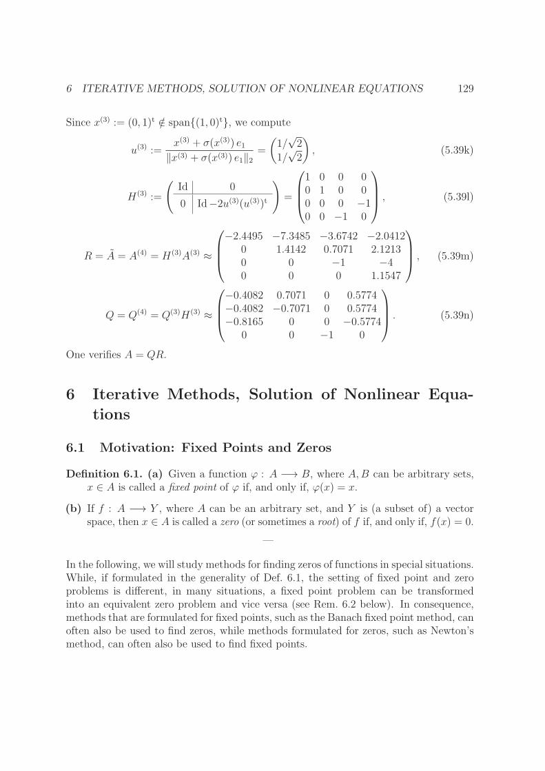
6 ITERATIVE METHODS, SOLUTION OF NONLINEAR EQUATIONS 129
Since x(3) := (0, 1)t /∈ span{(1, 0)t}, we compute
u(3) :=x(3) + σ(x(3)) e1‖x(3) + σ(x(3)) e1‖2
=
(1/√2
1/√2
), (5.39k)
H(3) :=
(Id 0
0 Id−2u(3)(u(3))t
)=
1 0 0 00 1 0 00 0 0 −10 0 −1 0
, (5.39l)
R = A = A(4) = H(3)A(3) ≈
−2.4495 −7.3485 −3.6742 −2.04120 1.4142 0.7071 2.12130 0 −1 −40 0 0 1.1547
, (5.39m)
Q = Q(4) = Q(3)H(3) ≈
−0.4082 0.7071 0 0.5774−0.4082 −0.7071 0 0.5774−0.8165 0 0 −0.5774
0 0 −1 0
. (5.39n)
One verifies A = QR.
6 Iterative Methods, Solution of Nonlinear Equa-
tions
6.1 Motivation: Fixed Points and Zeros
Definition 6.1. (a) Given a function ϕ : A −→ B, where A,B can be arbitrary sets,x ∈ A is called a fixed point of ϕ if, and only if, ϕ(x) = x.
(b) If f : A −→ Y , where A can be an arbitrary set, and Y is (a subset of) a vectorspace, then x ∈ A is called a zero (or sometimes a root) of f if, and only if, f(x) = 0.
—
In the following, we will study methods for finding zeros of functions in special situations.While, if formulated in the generality of Def. 6.1, the setting of fixed point and zeroproblems is different, in many situations, a fixed point problem can be transformedinto an equivalent zero problem and vice versa (see Rem. 6.2 below). In consequence,methods that are formulated for fixed points, such as the Banach fixed point method, canoften also be used to find zeros, while methods formulated for zeros, such as Newton’smethod, can often also be used to find fixed points.

6 ITERATIVE METHODS, SOLUTION OF NONLINEAR EQUATIONS 130
Remark 6.2. (a) If ϕ : A −→ B, where A,B are subsets of a common vector spaceX, then x ∈ A is a fixed point of ϕ if, and only if, ϕ(x)− x = 0, i.e. if, and only if,x is a zero of the function f : A −→ X, f(x) := ϕ(x)− x (we can no longer admitarbitrary sets A,B, as adding and subtracting must make sense; but note that itmight happen that ϕ(x)− x /∈ A ∪ B).
(b) If f : A −→ Y , where A and Y are both subsets of some common vector space Z,then x ∈ A is a zero of f if, and only if, f(x) + x = x, i.e. if, and only if, x is afixed point of the function ϕ : A −→ Z, ϕ(x) := f(x) + x.
—
Given a function g, an iterative method defines a sequence x0, x1, . . . , where, for n ∈ N0,xn+1 is computed from xn (or possibly x0, . . . , xn) by using g. For example, “using g”can mean applying g to obtain xn+1 := g(xn) or it can mean applying g and g′ in asuitable way (as in the case of Newton’s method according to (6.1) and (6.5) below).The iterative method with xn+1 := g(xn) is already known from the Banach fixed pointtheorem of Analysis 2 (cf. [Phi16b, Th. 2.29]). In the following, we will provide anintroduction to the iterative method known as Newton’s method.
6.2 Newton’s Method
As mentioned above, the Banach fixed point method has already been studied in Anal-ysis 2, [Phi16b, Sec. 2.2]. The Banach fixed point method has the advantage of beingapplicable in the rather general setting of a complete metric space and of not requiringany differentiability. Moreover, convergence results and error estimates are compara-tively simple to prove.
Newton’s method on the other hand is only applicable to differentiable maps betweennormed vector spaces and convergence results as well as error estimates are typicallyconsiderably more difficult to establish, especially in more than one dimension. However,if Newton’s method converges, than the convergence is typically considerably faster thanfor the Banach fixed point method and, hence, Newton’s method is preferred in suchsituations.
While the Banach fixed point method is designed to provide sequences that converge toa fixed point of a function ϕ, Newton’s method is designed to provide sequences thatconverge to a zero of a function f (cf. Sec. 6.1 above).
The subject of Newton’s and related methods is a vast field and we will only be ableto provide a brief introduction – see, e.g., [Deu11], [OR70, Sections 12.6,13.3,14.4] forfurther results regarding such methods.

6 ITERATIVE METHODS, SOLUTION OF NONLINEAR EQUATIONS 131
6.2.1 Newton’s Method in One Dimension
If A ⊆ R and f : A −→ R is differentiable, then Newton’s method is defined by therecursion
x0 ∈ A, xn+1 := xn −f(xn)
f ′(xn)for each n ∈ N0. (6.1)
There are clearly several issues with Newton’s method as formulated in (6.1):
(a) Is the derivative of f in xn invertible (i.e. nonzero in the case of (6.1))?
(b) Is xn+1 an element of A such that the iteration can be continued?
(c) Does the sequence (xn)n∈N0 converge?
To ensure that we can answer “yes” to all of the above questions, we need suitablehypotheses. The following theorem provides examples for sufficient conditions:
Theorem 6.3. Let I ⊆ R be a nontrivial interval (i.e. an interval consisting of morethan one point). Assume f : I −→ R to be differentiable with f ′(x) 6= 0 for each x ∈ Iand to have a zero x ∈ I. If f satisfies one of the following four conditions (a) – (d),then x is the only zero of f in I, and (6.1) well-defines a sequence (xn)n∈N0 in I thatconverges to x, provided that x0 = x (in which case the sequence is constant) or x0, x1are on different sides of x with x1 ∈ I or x0, x1 are on the same side of x (in which casethe sequence is monotone).
(a) f is strictly increasing and convex.
(b) f is strictly decreasing and concave.
(c) f is strictly increasing and concave.
(d) f is strictly decreasing and convex.
For (a) and (b), x0, x1 are on different sides of x for x0 < x and (xn)n∈N0 is decreasingfor x0 > x; for (c) and (d), x0, x1 are on different sides of x for x0 > x and (xn)n∈N0 isincreasing for x0 < x.
Proof. In each case, f is strictly monotone and, hence, injective. Thus, x must be theonly zero of f . For each n ∈ N0, if f(xn) = 0, then (6.1) implies xn+1 = xn, showing(xn)n∈N0 to be constant for x0 = x.

6 ITERATIVE METHODS, SOLUTION OF NONLINEAR EQUATIONS 132
We now assume (a). The convexity of f yields (cf. [Phi16a, (9.37)])
∀x,y∈I
f(x) ≥ f ′(y)(x− y) + f(y). (6.2)
We now apply (6.2) to x := xn+1 and y := xn, assuming n ∈ N0 with xn, xn+1 ∈ I,obtaining
f(xn+1) ≥ f ′(xn)(xn+1 − xn) + f(xn)(6.1)= 0. (6.3)
Claim 1. If (a) holds, then
η : I −→ R, η(x) := x− f(x)
f ′(x),
is increasing on [x, sup I[.
Proof. Let x1, x2 ∈ I such that x ≤ x1 < x2. Then we estimate
η(x2)− η(x1) = x2 − x1 +f(x1)
f ′(x1)− f(x2)
f ′(x2)
(6.2)
≥ f(x2)− f(x1)f ′(x2)
+f(x1)
f ′(x1)− f(x2)
f ′(x2)
= f(x1)
(1
f ′(x1)− 1
f ′(x2)
)≥ 0,
where we used f(x1) ≥ 0 (as f is increasing) and f ′(x1) ≤ f ′(x2) (as f is convex,[Phi16a, (9.37)]). N
If xn ∈ I with xn > x, then f(xn) > 0 (as f is strictly increasing) and f ′(xn) > 0 (as fis strictly increasing and f ′(xn) 6= 0), implying
x = η(x)Cl. 1
≤ η(xn) = xn+1 = xn −f(xn)
f ′(xn)< xn ⇒ xn+1 ∈ I. (6.4)
According to (6.4), if x0 ≥ x, then (xn)n∈N0 is a decreasing sequence in [x, x0], convergingto some x∗ ∈ [x, x0] (this is the case, where x0, x1 are on the same side of x). If x0 < xand x1 ∈ I, then (6.3) shows x1 ≥ x and, then, (6.4) yields (xn)n∈N is a decreasingsequence in [x, x1], converging to some x∗ ∈ [x, x1] (this is the case, where x0, x1 are ondifferent sides of x). In each case, we then obtain
x∗ = limn→∞
xn+1 = limn→∞
(xn −
f(xn)
f ′(xn)
)= x∗ −
f(x∗)
f ′(x∗),
proving f(x∗) = 0, i.e. x∗ = x (note that we did not assume the continuity of f ′ –however the boundedness of f ′ on [x, x1], as given by its monotonicity, already suffices
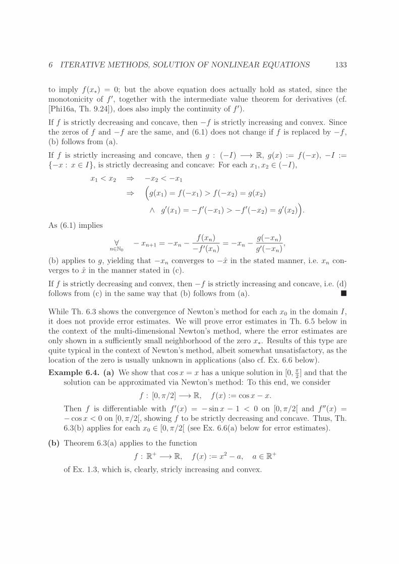
6 ITERATIVE METHODS, SOLUTION OF NONLINEAR EQUATIONS 133
to imply f(x∗) = 0; but the above equation does actually hold as stated, since themonotonicity of f ′, together with the intermediate value theorem for derivatives (cf.[Phi16a, Th. 9.24]), does also imply the continuity of f ′).
If f is strictly decreasing and concave, then −f is strictly increasing and convex. Sincethe zeros of f and −f are the same, and (6.1) does not change if f is replaced by −f ,(b) follows from (a).
If f is strictly increasing and concave, then g : (−I) −→ R, g(x) := f(−x), −I :={−x : x ∈ I}, is strictly decreasing and concave: For each x1, x2 ∈ (−I),
x1 < x2 ⇒ −x2 < −x1⇒
(g(x1) = f(−x1) > f(−x2) = g(x2)
∧ g′(x1) = −f ′(−x1) > −f ′(−x2) = g′(x2)).
As (6.1) implies
∀n∈N0
− xn+1 = −xn −f(xn)
−f ′(xn)= −xn −
g(−xn)g′(−xn)
,
(b) applies to g, yielding that −xn converges to −x in the stated manner, i.e. xn con-verges to x in the manner stated in (c).
If f is strictly decreasing and convex, then −f is strictly increasing and concave, i.e. (d)follows from (c) in the same way that (b) follows from (a). �
While Th. 6.3 shows the convergence of Newton’s method for each x0 in the domain I,it does not provide error estimates. We will prove error estimates in Th. 6.5 below inthe context of the multi-dimensional Newton’s method, where the error estimates areonly shown in a sufficiently small neighborhood of the zero x∗. Results of this type arequite typical in the context of Newton’s method, albeit somewhat unsatisfactory, as thelocation of the zero is usually unknown in applications (also cf. Ex. 6.6 below).
Example 6.4. (a) We show that cosx = x has a unique solution in [0, π2] and that the
solution can be approximated via Newton’s method: To this end, we consider
f : [0, π/2] −→ R, f(x) := cos x− x.Then f is differentiable with f ′(x) = − sin x − 1 < 0 on [0, π/2[ and f ′′(x) =− cos x < 0 on [0, π/2[, showing f to be strictly decreasing and concave. Thus, Th.6.3(b) applies for each x0 ∈ [0, π/2[ (see Ex. 6.6(a) below for error estimates).
(b) Theorem 6.3(a) applies to the function
f : R+ −→ R, f(x) := x2 − a, a ∈ R+
of Ex. 1.3, which is, clearly, stricly increasing and convex.

6 ITERATIVE METHODS, SOLUTION OF NONLINEAR EQUATIONS 134
6.2.2 Newton’s Method in Several Dimensions
Newton’s method, as defined in (6.1), naturally generalizes to a differentiable functionf : A −→ Rm, A ⊆ Rm, as follows:
x0 ∈ A, xn+1 := xn −(Df(xn)
)−1f(xn) for each n ∈ N0 (6.5)
(indeed, the same still works if Rm is replaced by some general normed vector space,but then the notion of differentiability needs to be generalized to such spaces, which isbeyond the scope of the present class).
In practice, in each step of Newton’s method (6.5), one will determine xn+1 as thesolution to the linear system
Df(xn)xn+1 = Df(xn)xn − f(xn). (6.6)
Not surprisingly, the issues formulated as (a), (b), (c) after (6.1) (i.e. invertibility ofDf(xn), xn+1 being in A, and convergence of (xn)n∈N0), are also present in the multi-dimensional situation.
As in the 1-dimensional case, we will present a result that provides an example for suffi-cient conditions for convergence (cf. Th. 6.5 below). While Th. 6.3 for the 1-dimensionalNewton’s method is an example of a global Newton theorem (proving convergence foreach x0 in the considered domain of f), Th. 6.5 is an example of a local Newton theorem,proving convergence under the assumption that x0 is sufficiently close to the zero x –however, in contrast to Th. 6.3, Th. 6.5 also includes error estimates (cf. (6.12), (6.13)).In the literature (e.g. in the previously mentioned references [Deu11], [OR70]), one findsmany variants of both local and global Newton theorems. A global Newton theorem inthe a multi-dimensional setting is also provided by Th. I.1 in the appendix.
Theorem 6.5. Let m ∈ N and fix a norm ‖ · ‖ on Rm. Let A ⊆ Rm be open. Moreoverlet f : A −→ A be differentiable, let x∗ ∈ A be a zero of f , and let r > 0 be (sufficientlysmall) such that
Br(x∗) ={x ∈ Rm : ‖x− x∗‖ < r
}⊆ A. (6.7)
Assume that Df(x∗) is invertible and that β > 0 is such that∥∥∥(Df(x∗)
)−1∥∥∥ ≤ β (6.8)
(here and in the following, we consider the induced operator norm on real n×n matrices).Finally, assume that the map Df : Br(x∗) −→ L(Rm,Rm) is Lipschitz continuous withLipschitz constant L ∈ R+, i.e.
∥∥(Df)(x)− (Df)(y)∥∥ ≤ L ‖x− y‖ for each x, y ∈ Br(x∗). (6.9)

6 ITERATIVE METHODS, SOLUTION OF NONLINEAR EQUATIONS 135
Then, letting
δ := min
{r,
1
2βL
}, (6.10)
Newton’s method (6.5) is well-defined for each x0 ∈ Bδ(x∗) (i.e., for each n ∈ N0,Df(xn) is invertible and xn+1 ∈ Bδ(x∗)), and
limn→∞
xn = x∗ (6.11)
with the error estimates
‖xn+1 − x∗‖ ≤ β L ‖xn − x∗‖2 ≤1
2‖xn − x∗‖, (6.12)
‖xn − x∗‖ ≤(1
2
)2n−1
‖x0 − x∗‖ (6.13)
for each n ∈ N0. Moreover, within Bδ(x∗), the zero x∗ is unique.
Proof. The proof is conducted via several steps.
Claim 1. For each x ∈ Bδ(x∗), the matrix Df(x) is invertible with
∥∥∥(Df(x)
)−1∥∥∥ ≤ 2β. (6.14)
Proof. Fix x ∈ Bδ(x∗). We will apply Lem. 2.45 with
A := Df(x∗), ∆A := Df(x)−Df(x∗), Df(x) = A+∆A. (6.15)
To apply Lem. 2.45, we must estimate ∆A. We obtain
‖∆A‖(6.9)
≤ L ‖x− x∗‖ < Lδ ≤ 1
2β
(6.8)
≤ 1
2‖A−1‖−1, (6.16)
such that we can, indeed, apply Lem. 2.45. In consequence, Df(x) is invertible with
∥∥∥(Df(x)
)−1∥∥∥
(2.32)
≤ ‖A−1‖1− ‖A−1‖ ‖∆A‖
(6.16)
≤ 2‖A−1‖ ≤ 2β, (6.17)
thereby establishing the case. N
Claim 2. For each x, y ∈ Br(x∗), the following holds:
∥∥f(x)− f(y)−Df(y)(x− y)∥∥ ≤ L
2‖x− y‖2. (6.18)

6 ITERATIVE METHODS, SOLUTION OF NONLINEAR EQUATIONS 136
Proof. We apply the chain rule to the auxiliary function
φ : [0, 1] −→ Rm, φ(t) := f(y + t(x− y)
)(6.19)
to obtainφ′(t) :=
(Df(y + t(x− y))
)(x− y) for each t ∈ [0, 1]. (6.20)
This allows us to write
f(x)− f(y)−Df(y)(x− y) = φ(1)− φ(0)− φ′(0) =
∫ 1
0
(φ′(t)− φ′(0)
)dt . (6.21)
Next, we estimate the norm of the integrand:
∥∥φ′(t)− φ′(0)∥∥ ≤
∥∥Df(y + t(x− y))−Df(y)∥∥ ‖x− y‖ ≤ L t ‖x− y‖2. (6.22)
Thus,
∥∥∥∥∫ 1
0
(φ′(t)− φ′(0)
)dt
∥∥∥∥ ≤∫ 1
0
∥∥φ′(t)− φ′(0)∥∥ dt ≤
∫ 1
0
L t ‖x− y‖2 dt =L
2‖x− y‖2.
(6.23)Combining (6.23) with (6.21) proves (6.18). N
We will now show thatxn ∈ Bδ(x∗) (6.24)
and the error estimate (6.12) holds for each n ∈ N0. We proceed by induction. Forn = 0, (6.24) holds by hypothesis. Next, we assume that n ∈ N0 and (6.24) holds.Using f(x∗) = 0 and (6.5), we write
xn+1 − x∗ = xn − x∗ −(Df(xn)
)−1(f(xn)− f(x∗)
)
= −(Df(xn)
)−1(f(xn)− f(x∗)−Df(xn)(xn − x∗)
). (6.25)
Applying the norm to (6.25) and using (6.14) and (6.18) implies
‖xn+1−x∗‖ ≤ 2 βL
2‖xn−x∗‖2 = β L ‖xn−x∗‖2 ≤ β L δ‖xn−x∗‖ ≤
1
2‖xn−x∗‖, (6.26)
which proves xn+1 ∈ Bδ(x∗) as well as (6.12).
Another induction shows that (6.12) implies, for each n ∈ N,
‖xn − x∗‖ ≤ (βL)1+2+···+2n−1‖x0 − x∗‖2n ≤ (βLδ)2
n−1‖x0 − x∗‖, (6.27)

6 ITERATIVE METHODS, SOLUTION OF NONLINEAR EQUATIONS 137
where the geometric sum formula 1+2+ · · ·+2n−1 = 2n−12−1
= 2n−1 was used for the last
inequality. Moreover, βLδ ≤ 12together with (6.27) proves (6.13), and, in particular,
(6.11).
Finally, we show that x∗ is the unique zero in Bδ(x∗): Suppose x∗, x∗∗ ∈ Bδ(x∗) withf(x∗) = f(x∗∗) = 0. Then
‖x∗∗ − x∗‖ =∥∥∥(Df(x∗)
)−1(f(x∗∗)− f(x∗)−Df(x∗)(x∗∗ − x∗)
)∥∥∥ . (6.28)
Applying (6.14) and (6.18) yields
‖x∗∗ − x∗‖ ≤ 2βL
2‖x∗ − x∗∗‖2 ≤ β L δ ‖x∗ − x∗∗‖ ≤
1
2‖x∗ − x∗∗‖, (6.29)
implying ‖x∗ − x∗∗‖ = 0 and completing the proof of the theorem. �
Example 6.6. (a) We already know from Ex. 6.4(a), that
f : [0, π/2] −→ R, f(x) := cos x− x,
has a unique zero x∗ ∈]0, π/2[ and that Newton’s method converges to x∗ for eachx0 ∈ [0, π/2[. Moreover,
∀x∈[0,π
2]
(−2 ≤ f ′(x) = − sin x− 1 ≤ −1 ⇒
∣∣∣∣1
f ′(x)
∣∣∣∣ ≤ 1
),
and f ′ is Lipschitz continuous with Lipschitz constant L = 1. Thus, Th. 6.5 applieswith β = L = 1. However, without further knowledge regarding the locationof the zero in [0, π/2], we do not have any lower positive bound on r to obtain
δ = min{r, 1
2βL
}. One possibility is to extend the domain to A :=] − 1
2, π2+ 1
2[,
yielding δ = r = 12βL
= 12. Thus, in combination with the information of Ex. 6.4(a),
we know that, for each x0 ∈ [0, π/2[, Newton’s method converges to the zero x∗and the error estimates (6.12), (6.13) hold if |x0−x∗| < 1
2(otherwise, (6.12), (6.13)
might not hold for some initial steps).
(b) Consider the map
f : R2 −→ R2, f
(x1x2
):=
(x1x2
)− 1
4
(cos x1 − sin x2cos x1 − 2 sin x2
).

6 ITERATIVE METHODS, SOLUTION OF NONLINEAR EQUATIONS 138
Then f is differentiable with, for each x =(x1
x2
)∈ R2,
Df(x) =1
4
(4 + sin x1 cos x2sin x1 4 + 2 cos x2
),
detDf(x) =1
16
(16 + 4 sin x1 + 8 cos x2 + sin x1 cos x2
)≥ 3
16> 0,
Df(x)−1 =1
detDf(x)
1
4
(4 + 2 cos x2 − cos x2− sin x1 4 + sin x1
).
We now consider R2 with ‖ · ‖∞ and recall from Ex. 2.18(a) that the row sum normis the corresponding operator norm. For each x, y ∈ R2, we estimate, using thatboth sin and cos are Lipschitz continuous with Lipschitz constant 1,
∥∥Df(x)−Df(y)∥∥∞ =
1
4
∥∥∥∥(| sin x1 − sin y1| | cos x2 − cos y2|| sin x1 − sin y1| 2| cos x2 − cos y2|
)∥∥∥∥∞
≤ 1
4
(|x1 − y1|+ 2|x2 − y2|
)≤ 3
4‖x− y‖∞,
as well as ∥∥Df(x)−1∥∥∞ ≤
16
3· 74· ‖x‖∞.
Thus, if we can establish f to have a zero in B1(0) = [−1, 1]× [−1, 1], then Th. 6.5applies with β := 28
3and L := 3
4(and arbitrary r ∈ R+), i.e. with δ = 1
2· 328· 43= 1
14.
To verify that f has a zero in B1(0), we note that f(x) = 0 is equivalent to thefixed point problem φ(x) = x with
φ : R2 −→ R2, φ
(x1x2
):=
1
4
(cos x1 − sin x2cos x1 − 2 sin x2
).
As φ, clearly, maps B1(0) (even all of R2) into B 34(0) and is a contraction, due to
∀x,y∈R2
∥∥φ(x)− φ(y)∥∥∞ ≤
3
4‖x− y‖∞,
the Banach fixed point theorem [Phi16b, Th. 2.29] applies, showing φ to have aunique fixed point x∗, which must be located in B 3
4(0). As we now only know Th.
6.5 to yield convergence of Newton’s method for x0 ∈ B 114(x∗), in practice, without
more accurate knowledge of the location of x∗, one could cover B 34(0) with squares
of side length 17, successively starting iterations in each of the squares, aborting an
iteration if one finds it to be inconsistent with the error estimates of Th. 6.5.

7 EIGENVALUES 139
7 Eigenvalues
7.1 Introductory Remarks
We recall some basic definitions and results from Linear Algebra: If A ∈M(n, F ) is ann × n matrix over the field F , n ∈ N, then λ ∈ F is called an eigenvalue of A if, andonly if,
∃06=v∈Fn
Av = λ v,
where every 0 6= v ∈ F n satisfying Av = λv is called an eigenvector to the eigenvalue λ.The set of all eigenvalues of A is called the spectrum of A, denoted σ(A). According to[Phi19b, Prop. 8.2(b)], σ(A) is precisely the set of zeros of the characteristic polynomialχA of A, where χA is defined by (cf. [Phi19b, Def. 8.1] and [Phi19b, Rem. 8.7(a)])
χA := det(X Idn−A) ∈ F [X].
For λ ∈ σ(A), its algebraic multiplicity ma(λ) and geometric multiplicity mg(λ) are (cf.[Phi19b, Def. 6.12] and [Phi19b, Th. 8.4]):
ma(λ) := ma(λ,A) := multiplicity of λ as a zero of χA,
mg(λ) := mg(λ,A) := dimker(A− λ Id).
Remark 7.1. Let F be a field, n ∈ N, A ∈M(n, F ).
(a) Eigenvalues of A and their multiplicities are invariant under similarity transforma-tions, i.e. if T ∈M(n, F ) is invertible and B := T−1AT , then σ(B) = σ(A) and, foreach λ ∈ σ(A), ma(λ,A) = ma(λ,B) as well as mg(λ,A) = mg(λ,B) (e.g. due tothe fact that χA and ker(A− λ Id) only depend on the linear maps (in L(F n, F n))represented by A and ker(A−λ Id), respectively, where A and B (resp. A−λ Id andT−1(A− λ Id)T ) represent the same map, merely with respect to different bases ofF n (cf. [Phi19b, Prop. 8.2(a)])).
(b) Note that the characteristic polynomial χA = det(X Idn−A) is always a monicpolynomial of degree n (i.e. a polynomial of degree n, where the coefficient of Xn is1, cf. [Phi19b, Rem. 8.3]). In general, the eigenvalues of A will be in the algebraicclosure F of F , cf. [Phi19b, Def. 7.11, Th. 7.38, Def. E.13, Th. E.16]3. On theother hand, every monic polynomial f ∈ F [X] of degree n ≥ 1 is the characteristic
3It is, perhaps, somewhat misleading to speak of the algebraic closure of F : Even though, accordingto [Phi19b, Cor. E.20], all algebraic closures of a given field F are isomorphic, the existence of theisomorphism is, in general, nonconstructive, based on an application of Zorn’s lemma.

7 EIGENVALUES 140
polynomial of some matrix A(f) ∈M(n, F ), where A(f) is the so-called companionmatrix of the polynomial: If a1, . . . , an ∈ F , and
f := Xn +n∑
j=1
aj Xn−j ,
then χA(f) = f for
A(f) :=
−a1 −a2 −a3 . . . −an−1 −an1 0
1 0
1. . .. . . 0
1 0
(cf. [Phi19b, Rem. 8.3(c)])). In the following, we will only consider matrices over Rand C, and we know that, due to the fundamental theorem of algebra (cf. [Phi16a,Th. 8.32]), C is the algebraic closure of R.
—
The computation of eigenvalues is of importance to numerous applications. A standardexample from Physics is the occurrance of eigenvalues as eigenfrequencies of oscillators.More generally, one often needs to compute eigenvalues when solving (linear) differentialequations (cf., e.g., [Phi16c, Th. 4.32, Rem. 4.51]). In this and many other applications,the occurrance of eigenvalues can be traced back to the fact that eigenvalues occurwhen transforming a matrix into suitable normal forms, e.g. into Jordan normal form(cf. [Phi19b, Th. 9.13]): To compute the Jordan normal form of a matrix, one firstneeds to compute its eigenvalues. For another example, recall that the computationof the spectral norm ‖A‖2 of a matrix A ∈ M(m,K) requires the computation of theabsolute value of an eigenvalue of A with maximal size (cf. Th. 2.24).
Remark 7.2. Given that eigenvalues are precisely the roots of the characteristic poly-nomial, and given that, as mentioned in Rem. 7.1(b), every monic polynomial of degreeat least 1 can occur as the characteristic polynomial of a matrix, it is not surprisingthat computing eigenvalues is, in general, a difficult task. According to Galois theoryin Algebra, for a generic polynomial of degree at least 5, it is not possible to obtainits zeros using so-called radicals (which are, roughly, zeros of polynomials of the formXk − λ, k ∈ N, λ ∈ F , see, e.g., [Bos13, Def. 6.1.1] for a precise definition) in finitelymany steps (cf., e.g., [Bos13, Cor. 6.1.7]) and, in general, an approximation by iterative
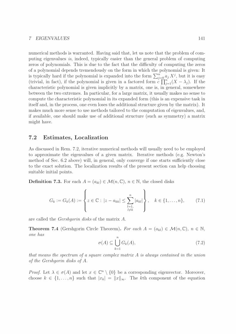
7 EIGENVALUES 141
numerical methods is warranted. Having said that, let us note that the problem of com-puting eigenvalues is, indeed, typically easier than the general problem of computingzeros of polynomials. This is due to the fact that the difficulty of computing the zerosof a polynomial depends tremendously on the form in which the polynomial is given: Itis typically hard if the polynomial is expanded into the form
∑nj=0 aj X
j, but it is easy(trivial, in fact), if the polynomial is given in a factored form c
∏nj=1(X − λj). If the
characteristic polynomial is given implicitly by a matrix, one is, in general, somewherebetween the two extremes. In particular, for a large matrix, it usually makes no sense tocompute the characteristic polynomial in its expanded form (this is an expensive task initself and, in the process, one even loses the additional structure given by the matrix). Itmakes much more sense to use methods tailored to the computation of eigenvalues, and,if available, one should make use of additional structure (such as symmetry) a matrixmight have.
7.2 Estimates, Localization
As discussed in Rem. 7.2, iterative numerical methods will usually need to be employedto approximate the eigenvalues of a given matrix. Iterative methods (e.g. Newton’smethod of Sec. 6.2 above) will, in general, only converge if one starts sufficiently closeto the exact solution. The localization results of the present section can help choosingsuitable initial points.
Definition 7.3. For each A = (akl) ∈M(n,C), n ∈ N, the closed disks
Gk := Gk(A) :=
z ∈ C : |z − akk| ≤
n∑
l=1,l 6=k
|akl|
, k ∈ {1, . . . , n}, (7.1)
are called the Gershgorin disks of the matrix A.
Theorem 7.4 (Gershgorin Circle Theorem). For each A = (akl) ∈ M(n,C), n ∈ N,one has
σ(A) ⊆n⋃
k=1
Gk(A), (7.2)
that means the spectrum of a square complex matrix A is always contained in the unionof the Gershgorin disks of A.
Proof. Let λ ∈ σ(A) and let x ∈ Cn \ {0} be a corresponding eigenvector. Moreover,choose k ∈ {1, . . . , n} such that |xk| = ‖x‖∞. The kth component of the equation

7 EIGENVALUES 142
Ax = λx reads
λxk =n∑
l=1
aklxl
and implies
|λ− akk| |xk| ≤n∑
l=1,l 6=k
|akl| |xl| ≤n∑
l=1,l 6=k
|akl| |xk|.
Dividing the estimate by |xk| 6= 0 shows λ ∈ Gk and, thus, proves (7.2). �
Corollary 7.5. For each A = (akl) ∈ M(n,C), n ∈ N, instead of using row sums todefine the Gershgorin disks of (7.1), one can use the column sums to define
G′k := G′
k(A) :=
z ∈ C : |z − akk| ≤
n∑
l=1,l 6=k
|alk|
, k ∈ {1, . . . , n}. (7.3)
Then one can strengthen the statement of Th. 7.4 to
σ(A) ⊆(
n⋃
k=1
Gk(A)
)∩(
n⋃
k=1
G′k(A)
). (7.4)
Proof. Since σ(A) = σ(At) and Gk(At) = G′
k(A), (7.4) is an immediate consequence of(7.2). �
Example 7.6. Consider the matrix
A :=
1 −1 02 −1 00 1 4
.
Then the Gershgorin disks according to (7.1) and (7.3) are (cf. Fig. 7.1)
G1 = B1(1), G2 = B2(−1), G3 = B1(4),
G′1 = B2(1), G′
2 = B2(−1), G′3 = {4}.
Here, the intersection of (7.4) is G1 ∪G2 ∪G′3 and, thus, noticeably smaller than either
G1 ∪G2 ∪G3 or G′1 ∪G′
2 ∪G′3 (cf. Fig. 7.1). The spectrum is
σ(A) = {−i, i, 4} :

7 EIGENVALUES 143
Figure 7.1: The Gershgorin disks of matrix A of Ex. 7.6 are depicted in the complexplane together with the exact locations of A’s eigenvalues: The black dots are thelocations of the eigenvalues, the grey disks are the rowwise disks G1, G2, G3, whereasthe columnwise disks G′
1, G′2, G
′3 are not shaded (only visible for G′
1, since G2 = G′2 and
G′3 = {4}).
Indeed, A is diagonalizable and, with T := 134
0 17 + 17i 17− 17i0 34i −34i4 −2− 8i −2 + 8i
,
T−1AT =1
2
2 3 172 −1− i 02 −1 + i 0
1 −1 02 −1 00 1 4
1
34
0 17 + 17i 17− 17i0 34i −34i4 −2− 8i −2 + 8i
=
4 0 00 −i 00 0 i
.
Figure 7.1 depicts the Gershgorin disks of A as well as the exact location of A’s eigen-values in the complex plane. Note that, while G3 contains precisely one eigenvalue, G1
contains none, and G2 contains 2.
Theorem 7.7. Let A = (akl) ∈M(n,C), n ∈ N. Suppose k1, . . . , kn is an enumerationof the numbers from 1 to n, and let q ∈ {1, . . . , n}. Moreover, suppose
D(1) = Gk1 ∪ · · · ∪Gkq (7.5a)
is the union of q Gershgorin disks of A and
D(2) = Gkq+1 ∪ · · · ∪Gkn (7.5b)
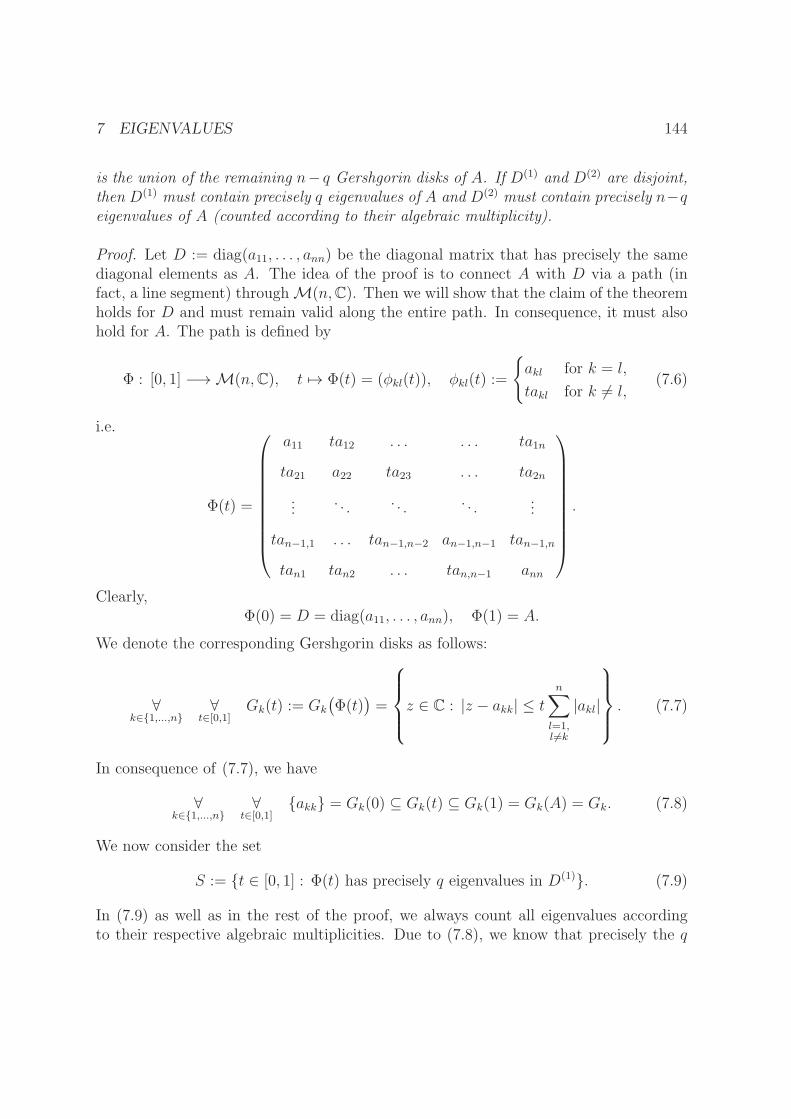
7 EIGENVALUES 144
is the union of the remaining n− q Gershgorin disks of A. If D(1) and D(2) are disjoint,then D(1) must contain precisely q eigenvalues of A and D(2) must contain precisely n−qeigenvalues of A (counted according to their algebraic multiplicity).
Proof. Let D := diag(a11, . . . , ann) be the diagonal matrix that has precisely the samediagonal elements as A. The idea of the proof is to connect A with D via a path (infact, a line segment) throughM(n,C). Then we will show that the claim of the theoremholds for D and must remain valid along the entire path. In consequence, it must alsohold for A. The path is defined by
Φ : [0, 1] −→M(n,C), t 7→ Φ(t) = (φkl(t)), φkl(t) :=
{akl for k = l,
takl for k 6= l,(7.6)
i.e.
Φ(t) =
a11 ta12 . . . . . . ta1n
ta21 a22 ta23 . . . ta2n
.... . . . . . . . .
...
tan−1,1 . . . tan−1,n−2 an−1,n−1 tan−1,n
tan1 tan2 . . . tan,n−1 ann
.
Clearly,Φ(0) = D = diag(a11, . . . , ann), Φ(1) = A.
We denote the corresponding Gershgorin disks as follows:
∀k∈{1,...,n}
∀t∈[0,1]
Gk(t) := Gk
(Φ(t)
)=
z ∈ C : |z − akk| ≤ t
n∑
l=1,l 6=k
|akl|
. (7.7)
In consequence of (7.7), we have
∀k∈{1,...,n}
∀t∈[0,1]
{akk} = Gk(0) ⊆ Gk(t) ⊆ Gk(1) = Gk(A) = Gk. (7.8)
We now consider the set
S := {t ∈ [0, 1] : Φ(t) has precisely q eigenvalues in D(1)}. (7.9)
In (7.9) as well as in the rest of the proof, we always count all eigenvalues accordingto their respective algebraic multiplicities. Due to (7.8), we know that precisely the q

7 EIGENVALUES 145
eigenvalues ak1k1 , . . . , akq ,kq of D are in D(1). In particular, 0 ∈ S and S 6= ∅. The proofis done once we show
τ := supS = 1 (7.10a)
andτ ∈ S (i.e. τ = maxS). (7.10b)
As D(1) and D(2) are compact and disjoint, they have a postive distance,
ǫ := dist(D(1), D(2)) > 0. (7.11)
Due to the continuous dependence of the eigenvalues on the coefficients of the matrix(cf. Cor. J.3 in the Appendix), there exists δ > 0 such that, for each s, t ∈ [0, 1]with |s − t| < δ, there exist enumerations λ1(s), . . . , λn(s) and λ1(t), . . . , λn(t) of theeigenvalues of Φ(s) and Φ(t), respectively, satisfying
∀k∈{1,...,n}
|λk(s)− λk(t)| < ǫ. (7.12)
Combining (7.12) with (7.11) yields
∀s,t∈[0,1]
((s ∈ S and |s− t| < δ) ⇒ t ∈ S
). (7.13)
Clearly, (7.13) implies both (7.10a) (since, otherwise, there were τ < t < 1 with |τ−t| <δ) and (7.10b) (since there are 0 < t < τ with |τ − t| < δ), thereby completing theproof. �
Remark 7.8. If A ∈ M(n,R), n ∈ N, then Th. 7.7 can sometimes help to determinewhich regions can contain nonreal eigenvalues: For real matrices all Gershgorin disksare centered on the real line. Moreover, if A is real, then λ ∈ σ(A) implies λ ∈ σ(A)and they must lie in the same Gershgorin disks (as they have the same distance to thereal line). Thus, if λ is not real, then it can not lie in any Gershgorin disks known tocontain just one eigenvalue.
Example 7.9. For the matrix A of Example 7.6, we see that the sets G1 ∪ G2 =B1(1) ∪ B2(−1) and G3 = B1(4) are disjoint (cf. Fig. 7.1). Thus, Th. 7.7 implies thatG3 contains precisely one eigenvalue and G1 ∪ G2 contains precisely two eigenvalues.Combining this information with Rem. 7.8 shows that G3 must contain a single realeigenvalue, whereas G1 ∪G2 could contain (as, indeed, it does) two conjugated nonrealeigenvalues.

7 EIGENVALUES 146
7.3 Power Method
Given an n × n matrix A ∈ M(n,C) and an initial vector z0 ∈ Cn, the power method(also known as power iteration or von Mises iteration) means applying increasinglyhigher powers of A to z0 according to the definition
zk := Azk−1 for each k ∈ N (i.e. zk = Ak z0 for each k ∈ N0). (7.14)
We will see below that this simple iteration can, in many situations and with suitablemodifications, be useful to approximate eigenvalues and eigenvectors (cf. Th. 7.12 andCor. 7.15 below). Before we can proof the main results, we need some preparation:
Proposition 7.10. The following holds true for each A ∈M(n,C), n ∈ N:
limk→∞
Ak = 0 ⇔ r(A) < 1, (7.15)
where r(A) denotes the spectral radius of A (cf. Def. 2.23).
Proof. First, suppose limk→∞Ak = 0. Let λ ∈ σ(A) and choose a corresponding eigen-vector v ∈ Cn \ {0}. Then, for each norm ‖ · ‖ on Cn with induced matrix norm onM(n,C),
∀k∈N
‖Akv‖ = ‖λkv‖ = |λ|k ‖v‖ ≤ ‖Ak‖ ‖v‖,
implying (since limk→∞ ‖Ak‖ = 0 and ‖v‖ > 0)
limk→∞|λ|k = 0,
which, in turn, implies |λ| < 1. Conversely, suppose r(A) < 1. If B, T ∈ M(n,C) andT is invertible with A = TBT−1, then an obvious induction shows
∀k∈N0
Ak = TBkT−1. (7.16)
According to [Phi19b, Th. 9.13], we can choose T such that (7.16) holds with B inJordan normal form, i.e. with B in block diagonal form
B =
B1 0
. . .
0 Br
, (7.17)
1 ≤ r ≤ n, where
Bj = (λj) or Bj =
λj 1 0 . . . 0λj 1
. . . . . . 00 λj 1
λj
,
7 EIGENVALUES 147
λj ∈ σ(A), Bj ∈ M(nj,C), nj ∈ {1, . . . , n} for each j ∈ {1, . . . , r}, and∑r
j=1 nj = n.Using blockwise matrix multiplication (cf. [Phi19a, Sec. 7.5]) in (7.17) yields
∀k∈N0
Bk =
Bk
1 0. . .
0 Bkr
. (7.18)
We now show∀
j∈{1,...,r}limk→∞
Bkj = 0. (7.19)
To this end, we write Bj = λj Id+Nj, where Nj ∈ M(nj ,C) is a canonical nilpotentmatrix,
Nj = 0 (zero matrix) or Nj =
0 1 0 . . . 00 1
. . . . . . 0
0 0 1
0
,
and apply the binomial theorem to obtain
∀k∈N
Bkj =
k∑
α=0
(k
α
)λk−αj Nα
j
Nnjj =0=
min{k,nj−1}∑
α=0
(k
α
)λk−αj Nα
j . (7.20)
Using
∀k∈N
∀α∈{0,...,k}
(k
α
)=
k!
α! (k − α)! ≤ k(k − 1) · · · (k − α + 1) ≤ kα,
and an arbitrary induced matrix norm onM(n,C), (7.20) implies
‖Bkj ‖ ≤
nj−1∑
α=0
kα|λj|k−α‖Nj‖α|λj |<1→ 0 for k →∞,
proving (7.19). Next, we conclude limk→∞Bk = 0 from (7.18). Thus, as ‖Ak‖ ≤‖T‖ ‖Bk‖ ‖T−1‖, the claimed limk→∞Ak = 0 also follows and completes the proof. �
Definition 7.11. Let A ∈ M(n,C), z ∈ Cn, n ∈ N. Recalling from [Phi19b, Th.9.13(a)] that Cn is the direct sum of the generalized eigenspaces of A,
Cn =⊕
λ∈σ(A)
M(λ), ∀λ∈σ(A)
M(λ) :=M(λ,A) := ker(A− λ Id)ma(λ), (7.21)

7 EIGENVALUES 148
we say that z has a nontrivial part in M(µ), µ ∈ σ(A), if, and only if, in the uniquedecomposition of z with respect to the direct sum (7.21),
z =∑
λ∈σ(A)
zλ with zµ 6= 0, ∀λ∈σ(A)
zλ ∈M(λ). (7.22)
Theorem 7.12. Let A ∈ M(n,C), n ∈ N. Suppose that A has an eigenvalue that islarger in size than all other eigenvalues of A, i.e.
∃λ∈σ(A)
∀µ∈σ(A)\{λ}
|λ| > |µ|. (7.23)
Moreover, assume λ to be semisimple (i.e. A↾M(λ) is diagonalizable and all Jordan blockswith respect to λ are trivial). Choosing an arbitrary norm ‖ · ‖ on Cn and starting withz0 ∈ Cn, define the sequence (zk)k∈N0 via the power iteration (7.14). From the zk alsodefine sequences (wk)k∈N0 and (αk)k∈N0 by
wk :=
{zk
‖zk‖ for zk 6= 0,
z0 for zk = 0∈ Cn for each k ∈ N0, (7.24a)
αk :=
{z∗k Azkz∗k zk
for zk 6= 0,
0 for zk = 0∈ C for each k ∈ N0 (7.24b)
(treating the zk as column vectors). If z0 has a nontrivial part in M(λ) in the sense ofDef. 7.11, then
limk→∞
αk = λ (7.25a)
and there exist sequences (φk)k∈N in R and (rk)k∈N in Cn such that, for all k sufficientlylarge,
wk = eiφkvλ + rk‖vλ + rk‖
, ‖vλ + rk‖ 6= 0, limk→∞
rk = 0, (7.25b)
where vλ is an eigenvector corresponding to the eigenvalue λ.
Proof. If λ = 0, then condition (7.23) together with λ being semisimple implies A = 0and there is nothing to prove. Thus, we proceed under the assumption λ 6= 0. As in theproof of Prop. 7.10, we choose T ∈ M(n,C) invertible such that (7.16) holds with Bin Jordan normal form. However, this time, we choose T such that the (trivial) Jordanblocks corresponding to λ come first, i.e.
B =
B1 0B2
. . .
0 Br
, B1 = λ Id ∈M(n1,C), (7.26)

7 EIGENVALUES 149
Bj ∈ M(nj ,C), is a Jordan matrix to λj ∈ σ(A) \ {λ} for each j = 2, . . . , r, r ∈{1, . . . , n}, n1, . . . , nr ∈ N, where
∑rj=1 nj = n. Since T is invertible, the columns
t1, . . . , tn of T form a basis of Cn. For each j ∈ {1, . . . , n1}, we compute
Atj = TBT−1tj = TBej = Tλej = λtj, (7.27)
showing tj to be an eigenvector corresponding to λ. Thus, t1, . . . , tn1 form a basis ofM(λ) = ker(A− λ Id) (here, the eigenspace is the same as the generalized eigenspace),and, if z0 has a nontrivial part in M(λ), then there exist ζ1, . . . , ζn ∈ C with at leastone ζj 6= 0, j ∈ {1, . . . , n1}, such that
z0 = vλ +n∑
j=n1+1
ζj tj, vλ =
n1∑
j=1
ζj tj.
We note vλ to be an eigenvector corresponding to λ. Next, we compute, for each k ∈ N0,
Ak z0 = TBkT−1
(vλ +
n∑
j=n1+1
ζj tj
)= λkvλ + TBk
(n∑
j=n1+1
ζj ej
)
= λk
(vλ + T
1
λkBk
(n∑
j=n1+1
ζj ej
)), (7.28)
where, in the last step, we have used λ 6= 0. In consequence, letting, for each k ∈ N0,
rk := T1
λkBk
(n∑
j=n1+1
ζj ej
), (7.29)
we obtain, for each k such that vλ + rk 6= 0,
wk =Ak z0‖Ak z0‖
=λk
|λ|kvλ + rk‖vλ + rk‖
. (7.30)
Let βk := λk
|λ|k . Then |βk| = 1 and, thus, there is φk ∈ [0, 2π[ such that βk = eiφk . To
prove (7.25b), it now only remains to show limk→∞ rk = 0. However, the hypothesis(7.23) implies
∀j∈{2,...,r}
r
(1
λBj
)=|λj||λ| < 1
and Prop. 7.10, in turn, implies limk→∞1λkB
kj = 0. Using this in (7.29), where 1
λkBk is
applied to a vector in span{en1+1, . . . , en}, yields
limk→∞
rk = T limk→∞
1
λkBk
(n∑
j=n1+1
ζj ej
)= 0, (7.31)

7 EIGENVALUES 150
finishing the proof of (7.25b). Finally, it is
limk→∞
αk = limk→∞
z∗k Azkz∗k zk
= limk→∞
w∗k Awk
w∗k wk
= limk→∞
(v∗λ + r∗k)A(vλ + rk)
(v∗λ + r∗k)(vλ + rk)=λv∗λvλv∗λvλ
= λ,
establishing (7.25a) and completing the proof. �
Caveat 7.13. It is emphasized that, due to the presence of the factor eiφk , (7.25b) doesnot claim the convergence of the wk to an eigenvector of λ. Indeed, in general, thesequence (wk)k∈N cannot be expected to converge. However, as vλ is an eigenvector for
λ, so is every eiφk‖vλ+rk‖ vλ (and every other scalar multiple). Thus, what (7.25b) does claim
is that, for sufficiently large k, wk is arbitrarily close to an eigenvector of λ, namely to
the eigenvector eiφk vλ‖vλ‖ (the eigenvector that wk is close to still depends on k).
Remark 7.14. (a) The hypothesis of Th. 7.12, that z0 have a nontrivial part inM(λ),can be difficult to check in practice. Still, it is usually not a severe restriction: Evenif, initially, z0 does not satisfy the condition, roundoff errors during the computationof the zk = Akz0 will cause the condition to be satisfied for sufficiently large k.
(b) The rate of convergence of the rk in Th. 7.12 (and, thus, of the αk as well) isdetermined by the size of |µ|/|λ|, where µ is a second largest eigenvalue (in termsof absolute value). Therefore, the convergence will be slow if |µ| and |λ| are close.
—
Even though the power method applied according to Th. 7.12 will (under the hypothesisof the theorem) only approximate the dominant eigenvalue (i.e. the largest in terms ofabsolute value), the following modification, known as the inverse power method, can beused to approximate other eigenvalues:
Corollary 7.15. Let A ∈M(n,C), n ∈ N, and assume λ ∈ σ(A) to be semisimple. Letp ∈ C \ {λ} be closer to λ than to any other eigenvalue of A, i.e.
∀µ∈σ(A)\{λ}
0 < |λ− p| < |µ− p|. (7.32)
SetG := (A− p Id)−1. (7.33)
Choosing an arbitrary norm ‖ · ‖ on Cn and starting with z0 ∈ Cn \ {0}, define thesequence (zk)k∈N0 via the power iteration (7.14) with A replaced by G. From the zk also

7 EIGENVALUES 151
define sequences (wk)k∈N0 and (αk)k∈N0 by
wk :=zk‖zk‖
=Gkz0‖Gkz0‖
∈ Cn for each k ∈ N0, (7.34a)
αk :=
{z∗k zkz∗k Gzk
+ p for z∗k Gzk 6= 0,
0 otherwise∈ C for each k ∈ N0 (7.34b)
(treating the zk as column vectors). If z0 has a nontrivial part in M((λ − p)−1, G) inthe sense of Def. 7.11, then
limk→∞
αk = λ (7.35a)
and there exist sequences (φk)k∈N in R and (rk)k∈N in Cn such that, for all k sufficientlylarge,
wk = eiφkvλ + rk‖vλ + rk‖
, ‖vλ + rk‖ 6= 0, limk→∞
rk = 0, (7.35b)
where vλ is an eigenvector corresponding to the eigenvalue λ.
Proof. First note that (7.32) implies p /∈ σ(A), such that G is well-defined. As G isinvertible, z0 6= 0 implies Gkz0 6= 0 for each k ∈ N0, showing the wk to be well-definedas well. The idea is to apply Th. 7.12 to G. Let µ ∈ C \ {p} and v ∈ Cn \ {0}. Then
Av = µv
⇔ (µ− p) v = (A− p Id) v⇔ (A− p Id)−1 v = (µ− p)−1 v, (7.36)
showing µ to be an eigenvalue for A with corresponding eigenvector v if, and only if,(µ−p)−1 is an eigenvalue for G = (A−p Id)−1 with the same corresponding eigenvectorv. In particular, (7.32) implies 1
λ−pto be the dominant eigenvalue of G. Next, notice
that the hypothesis that λ be semisimple for A implies M(λ,A) to have a basis ofeigenvectors v1, . . . , vn1 , n1 = ma(λ) (cf. (7.21)), which, by (7.36), then constitutes abasis of eigenvectors for M( 1
λ−p, G) as well, showing 1
λ−pto be semisimple for G. Thus,
all hypotheses of Th. 7.12 are satisfied and we obtain limk→∞ αk = (λ − p) + p = λ,proving (7.35a). Moreover, (7.35b) also follows, where vλ is an eigenvector for 1
λ−pand
G. However, then vλ is also an eigenvector for λ and A by (7.36). �
Remark 7.16. In practice, one computes the zk for the inverse power method of Cor.7.15 by solving the linear systems (A−p Id)zk = zk−1 for zk. As the matrix A−p Id doesnot vary, but only the right-hand side of the system varies, one should solve the systemsby first computing a suitable decomposition of A − p Id (e.g. a QR decomposition, cf.Rem. 5.15).

7 EIGENVALUES 152
Remark 7.17. In sufficiently benign situations (say, if A is diagonalizable and alleigenvalues are in R+
0 , e.g., if A is Hermitian), one can combine the inverse power method(IPM) of Cor. 7.15 with a bisection (or similar) method to obtain all eigenvalues of A:One starts by determining upper and lower bounds for σ(A) ⊆ [m,M ] (for example,by using Cor. 7.5). One then chooses p := (m+M)/2 as the midpoint and determinesλ = λ(p). Next, one uses the midpoints p1 := (m + p)/2 and p2 := (p +M)/2 anditerates the method, always choosing the midpoints of previous intervals. For each newmidpoint p, four possibilities can occur: (i) one finds a new eigenvalue by IPM , (ii) IPMfinds an eigenvalue that has already been found before, (iii) IPM fails, since p itself is aneigenvalue, (iv) IPM fails since p is exactly in the middle between two other eigenvalues.Cases (iii) and (iv) are unlikely, but if they do occur, they need to be recognized andtreated separately. If not all eigenvalues are real, one can still use an analogous method,one just has to cover a certain compact section of the complex plane by finer and finergrids. If one were to use squares for the grids, one could use the centers of the squaresto replace the midpoints of the intervals in the described procedure.
7.4 QR Method
The QR algorithm for the approximation of the eigenvalues of A ∈M(n,K) makes useof the QR decomposition A = QR of A into a unitary matrix Q and an upper triangularmatrix R (cf. Def. 5.12(a)). We already know from Th. 5.24 that Q and R can beobtained via the Householder method of Def. 5.23.
Algorithm 7.18 (QR Method). Given A ∈ M(n,K), n ∈ N, we define the followingalgorithm for the computation of a sequence (A(k))k∈N of matrices in M(n,K): LetA(1) := A. For each k ∈ N, let
A(k+1) := RkQk, (7.37a)
where
A(k) = QkRk (7.37b)
is a QR decomposition of A(k).
Remark 7.19. In each step of the QR method of Alg. 7.18, one needs to obtain a QRdecomposition of A(k). For a fully populated matrix A(k), the complexity of obtaining aQR decomposition is O(n3) (obtaining a QR decomposition via the Householder methodof Def. 5.23 requires O(n) matrix multiplications, each matrix multiplication needingO(n2) multiplications). The complexity can be improved to O(n2) by first transformingA into so-called Hessenberg form (the complexity of the transformation is O(n3), cf.

7 EIGENVALUES 153
Sections J.2 and J.3 of the Appendix). Thus, in practice, it is always advisable totransform A into Hessenberg form before applying the QR method.
Lemma 7.20. Let A ∈ M(n,K), n ∈ N. Moreover, for each k ∈ N, let matricesA(k), Rk, Qk ∈ M(n,K) be defined according to Alg. 7.18. Then the following identitieshold for each k ∈ N:
A(k+1) = Q∗k A
(k)Qk, (7.38a)
A(k+1) = (Q1Q2 · · ·Qk)∗A (Q1Q2 · · ·Qk), (7.38b)
Ak = (Q1Q2 · · ·Qk)(RkRk−1 · · ·R1). (7.38c)
Proof. (7.38a) holds, as
∀k∈N
Q∗k A
(k)Qk = Q∗kQk RkQk = RkQk = A(k+1).
A simple induction applied to (7.38a) yields (7.38b). Another induction yields (7.38c):For k = 1, it is merely (7.37b). For k ∈ N, we compute
Q1 · · ·Qk
A(k+1)
︷ ︸︸ ︷Qk+1Rk+1Rk · · ·R1
(7.38b)=
Id︷ ︸︸ ︷(Q1 · · ·Qk)(Q1 · · ·Qk)
∗ A (Q1 · · ·Qk)(Rk · · ·R1)ind. hyp.= AAk = Ak+1,
which completes the induction and establishes the case. �
In the following Th. 7.22, it will be shown that, under suitable hypotheses, the matricesA(k) of the QR method become, asymptotically, upper triangular, with the diagonalentries converging to the eigenvalues of A. Theorem 7.22 is not the most general con-vergence result of this kind. We will remark on possible extensions afterwards and wewill also indicate that some of the hypotheses are not as restrictive as they might seemat first glance.
Notation 7.21. Let n ∈ N. By diag(λ1, . . . , λn) we denote the diagonal n × n matrixwith diagonal entries λ1, . . . , λn, i.e.
diag(λ1, . . . , λn) := D = (dkl), dkl :=
{λk for k = l,
0 for k 6= l
(we have actually used this notation before). If A = (akl) is an n × n matrix, then,by diag(A), we denote the diagonal n × n matrix that has precisely the same diagonalentries as A, i.e.
diag(A) := D = (dkl), dkl :=
{akk for k = l,
0 for k 6= l.

7 EIGENVALUES 154
Theorem 7.22. Let A ∈ M(n,K), n ∈ N. Assume A to be diagonizable, invertible,and such that all eigenvalues λ1, . . . , λn ∈ σ(A) ⊆ K are distinct, satisfying
|λ1| > |λ2| > · · · > |λn| > 0. (7.39a)
Let T ∈M(n,K) be invertible and such that
A = TDT−1, D := diag(λ1, . . . , λn). (7.39b)
Assume T−1 to have an LU decomposition (without permutations), i.e., assume
T−1 = LU, (7.39c)
where L,U ∈ M(n,K), L being unipotent and lower triangular, U being upper trian-gular. If (A(k))k∈N is defined according to Alg. 7.18, then the A(k) are, asymptotically,upper triangular, with the diagonal entries converging to the eigenvalues of A, i.e.
∀j,l∈{1,...,n},
j>l
limk→∞
a(k)jl = 0 (7.40a)
and∀
j∈{1,...,n}limk→∞
a(k)jj = λj. (7.40b)
Moreover, there exists a constant C > 0, such that we have the error estimates
∀k∈N
∀
j,l∈{1,...,n},j>l
∣∣∣a(k)jl
∣∣∣ ≤ C qk, ∀j∈{1,...,n}
∣∣∣a(k)jj − λj∣∣∣ ≤ C qk
, (7.40c)
where
q := max
{ |λj+1||λj|
: j ∈ {1, . . . , n− 1}}< 1. (7.40d)
Proof. For n = 1, there is nothing to prove (one has A = D = A(k) for each k ∈ N).Thus, we assume n > 1 for the rest of the proof. We start by making a number ofobservations for k ∈ N being fixed. From (7.38c), we obtain a QR decomposition of Ak:
Ak = Qk Rk, Qk := Q1 · · ·Qk, Rk := Rk · · ·R1. (7.41)
On the other hand, we also have
Ak = TDkLU = XkDkU, Xk := TDkLD−k. (7.42)
We note Xk to be invertible, as it is the product of invertible matrices. Thus Xk has aQR decompositionXk = QXk
RXkwith invertible upper triangular matrix RXk
. Plugging

7 EIGENVALUES 155
the QR decomposition of Xk into (7.42), thus, yields a second QR decomposition of Ak,namely
Ak = QXk(RXk
DkU).
Due to Prop. 5.13, we now obtain a unitary diagonal matrix Sk such that
Qk = QXkSk, Rk = S∗
kRXkDkU. (7.43)
This will now allow us to compute a somewhat complicated-looking representation ofA(k), which, nonetheless, will turn out to be useful in advancing the proof: We have, fork ≥ 2,
Qk = (Q1 · · ·Qk−1)−1(Q1 · · ·Qk−1Qk) = Q−1
k−1Qk = S∗k−1Q
−1Xk−1
QXkSk,
Rk = (RkRk−1 · · ·R1)(Rk−1 · · ·R1)−1 = RkR
−1k−1
= S∗kRXk
DkUU−1D−(k−1)R−1Xk−1
Sk−1 = S∗kRXk
DR−1Xk−1
Sk−1,
implying
A(k) (7.37b)= QkRk = S∗
k−1Q−1Xk−1
QXkRXk
DR−1Xk−1
Sk−1
= S∗k−1RXk−1
R−1Xk−1
Q−1Xk−1
QXkRXk
DR−1Xk−1
Sk−1
= S∗k−1RXk−1
X−1k−1XkDR
−1Xk−1
Sk−1. (7.44)
The next step is to investigate the entries of
Xk = TL(k), L(k) := DkLD−k. (7.45)
As L is lower triangular with ljj = 1, we have
l(k)jl = λkj ljl λ
−kl =
0 for j < l,
1 for j = l,
ljl (λj
λl)k for j > l,
and
|l(k)jl |
= 0 for j < l,
= 1 for j = l,
≤ CL qk for j > l,
where q is as in (7.40d) and
CL := max{|ljl| : l, j ∈ {1, . . . , n}}.

7 EIGENVALUES 156
Thus, there is a lower triangular matrix Ek and a constant CE ∈ R+ such that
L(k) = Id+Ek, ‖Ek‖2 ≤ CECL qk. (7.46)
ThenXk = TL(k) = T + TEk. (7.47)
Set, for k ≥ 2,Fk := (Ek − Ek−1) (Id+Ek−1)
−1. (7.48)
As limk→∞Ek = 0, the sequence(‖(Id+Ek−1)
−1‖2)k∈N is bounded, i.e. there is a con-
stant CF > 0 such that
∀k≥2
‖Fk‖2 ≤∥∥Ek − Ek−1
∥∥2
∥∥(Id+Ek−1)−1∥∥2≤ CECL (q
k + qk−1)CF ≤ C1 qk,
C1 := 2CECLCF q−1 (note q > 0).
Now (7.48) is equivalent to
Id+Ek = (Id+Ek−1) (Id+Fk),
implying
X−1k−1Xk = (T + TEk−1)
−1(T + TEk) = (Id+Ek−1)−1(Id+Ek) = Id+Fk.
Plugging the last equality into (7.44) yields
A(k) = S∗k−1RXk−1
(Id+Fk)DR−1Xk−1
Sk−1
= S∗k−1RXk−1
DR−1Xk−1
Sk−1︸ ︷︷ ︸=:A
(k)D
+S∗k−1RXk−1
FkDR−1Xk−1
Sk−1︸ ︷︷ ︸=:A
(k)F
. (7.49)
To estimate ‖A(k)F ‖2, we note
‖RXk‖2 = ‖Q∗
XkXk‖2 = ‖Xk‖2, ‖R−1
Xk‖2 = ‖X−1
k QXk‖2 = ‖X−1
k ‖2,since QXk
is unitary and, thus, isometric. Due to (7.46) and (7.47), limk→∞Xk = T ,such that the sequences (‖RXk
‖2)k∈N and (‖R−1Xk‖2)k∈N are bounded by some constant
CR > 0. Thus, as the Sk are also unitary,
∀k≥2
‖A(k)F ‖2 =
∥∥∥S∗k−1RXk−1
FkDR−1Xk−1
Sk−1
∥∥∥2≤ C2
R‖D‖2C1 qk. (7.50)
Next, we observe each A(k)D to be an upper triangular matrix, as it is the product of
upper triangular matrices. Moreover, each Sk is a diagonal matrix and diag(RXk)−1 =
diag(R−1Xk
). Thus,
∀k≥2
diag(A(k)D ) = S∗
k−1 diag(RXk−1)D diag(R−1
Xk−1)Sk−1 = D. (7.51)
Finally, as we know the 2-norm onM(n,K) to be equivalent to the max-norm on Kn2,
combining (7.49) – (7.51) proves everything that was claimed in (7.40). �

7 EIGENVALUES 157
Remark 7.23. (a) Hypothesis (7.39c) of Th. 7.22 that T−1 has an LU decompositionwithout permutations is not as severe as it may seem. If permutations are necessaryin the LU decomposition of T−1, then Th. 7.22 and its proof remain the same,except that the eigenvalues will occur permuted in the limiting diagonal matrix D.Moreover, it is an exercise to show that, if the matrix A in Th. 7.22 has Hessenbergform with 0 /∈ {a21, . . . , an,n−1} (in view of Rem. 7.19, this is the case of mostinterest), then hypothesis (7.39c) can always be satisfied: As a intermediate step,one can show that, in this case,
∀j∈{1,...,n−1}
span{e1, . . . , ej} ∩ span{tj+1, . . . , tn} = {0},
where e1, . . . , en−1 are the standard unit vectors, and t1, . . . , tn are the eigenvectorsof A that form the columns of T .
(b) If A has several eigenvalues of equal modulus (e.g. multiple eigenvalues or nonrealeigenvalues of a real matrix), then the sequence of the QR method can no longerbe expected to be asymptotically upper triangular, only block upper triangular. Forexample, if |λ1| = |λ2| > |λ3| = |λ4| = |λ5|, then the asymptotic form will look like
∗ ∗ ∗ ∗ ∗∗ ∗ ∗ ∗ ∗
∗ ∗ ∗∗ ∗ ∗∗ ∗ ∗
,
where the upper diagonal 2×2 block still has eigenvalues λ1, λ2 and the lower diag-onal 3× 3 block still has eigenvalues λ3, λ4, λ5 (see [Cia89, Sec. 6.3] and referencestherein).
Remark 7.24. (a) The efficiency of the QR method can be improved significantly bythe introduction of so-called spectral shifts. One replaces (7.37) by
A(k+1) := RkQk + µk Id, (7.52a)
where
A(k) − µk Id = QkRk (7.52b)
is a QR decomposition of A(k) − µk Id and µk ∈ C is the shift parameter of the kthstep. As it turns out, using the lowest diagonal entry of the previous iteration asshift parameter, µk := a
(k)nn , is a simple choice that yields good results (see [SK11,
8 MINIMIZATION 158
Sec. 5.5.2]). According to [HB09, Sec. 27.3], an even better choice, albeit less simple,is to choose µk as the eigenvalue of
(a(k)n−1,n−1 a
(k)n−1,n
a(k)n,n−1 a
(k)nn
)
that is closest to a(k)nn . If one needs to find nonreal eigenvalues of a real matrix, the
related strategy of so-called double shifts is warranted (see [SK11, Sec. 5.5.3]).
(b) The above-described QR method with shifts is particularly successful if applied toHessenberg matrices in combination with a strategy known as deflation. After eachstep, each element of the first subdiagonal is tested if it is sufficiently close to 0 to betreated as “already converged”, i.e. to be replaced by 0. Then, if a
(k)j,j−1, 2 ≤ j ≤ n,
has been replaced by 0, the QR method is applied separately to the upper diagonal(j − 1) × (j − 1) block and the lower diagonal (n − j + 1) × (n − j + 1) block. Ifj = 2 or j = n (this is what usually happens if the shift strategy as described in (a)
is applied), then a(k)11 = λ1 or a
(k)nn = λn is already correct and one has to continue
with an (n− 1)× (n− 1) matrix.
8 Minimization
8.1 Motivation, Setting
Minimization (more generally, optimization) is a vast field, and we can only cover a fewselected aspects in this class. We will consider minimization problems of the form
min f(a), f : A −→ R. (8.1)
The function f to be minimized is often called the objective function or the objectivefunctional of the problem, even though this seems to be particularly common in thecontext of constrained minimization (see below).
In Sec. 6.1, we discussed the tasks of finding zeros and fixed points of functions, and wefound that, in most situations, both problems are equivalent. Minimization provides athird perspective onto this problem class: If F : A −→ Y , where (Y, ‖ · ‖) is a normedvector space, and α > 0, then
F (x) = 0 ⇔ ‖F (x)‖α = 0 = min{‖F (a)‖α : a ∈ A}.More generally, given y ∈ Y , we have the equivalence
F (x) = y ⇔ ‖F (x)− y‖α = 0 = min{‖F (a)− y‖α : a ∈ A}. (8.2)

8 MINIMIZATION 159
However, minimization is more general: If we seek the (global) min of the functionf : A −→ R, f(a) := ‖F (a) − y‖α, then it will yield a solution to F (x) = y, providedsuch a solution exists. On the other hand, f can have a minimum even if F (x) = ydoes not have a solution. If Y = Rn, n ∈ N, with the 2-norm, and α = 2, then theminimization of f is known as a least squares problem. The least squares problem iscalled linear if A is a normed vector space over R and F : A −→ Y is linear, andnonlinear otherwise.
One distinguishes between constrained and unconstrained minimization, where con-strained minimization can be seen as restricting the objective function f : A −→ R
to some subset of A, determined by the constraints. Constraints can be given explic-itly or implicitly. If A = R, then an explicit constraint might be to seek nonnegativesolutions. Implicit constraints can be given in the form of equation constraints – forexample, if A = Rn, then one might want to minimize f on the set of all solutions toMa = b, where M is some real m × n matrix. In this class, we will restrict ourselvesto unconstrained minimization. In particular, we will not cover the simplex method, amethod for so-called linear programming, which consists of minimizing a linear f withaffine constraints in finite dimensions (see, e.g., [HH92, Sec. 9] or [Str08, Sec. 5]). Forconstrained nonlinear optimization see, e.g., [QSS07, Sec. 7.3]). The optimal control ofdifferential equations is an example of constrained minimization in infinite dimensions(see, e.g., [Phi09]).
We will only consider methods that are suitable for unconstrained nonlinear minimiza-tion, noting that even the linear least squares problem is a nonlinear minimization prob-lem. Both methods involving derivatives (such as gradient methods) and derivative-freemethods are of interest. Derivative-based methods typically show faster convergencerates, but, on the other hand, they tend to be less robust, need more function evalua-tions (i.e. each step of the method is more costly), and have a smaller scope of applica-bility (e.g., the function to be minimized must be differentiable). Below, we will studyderivative-based methods in Sections 8.3 and 8.4, whereas derivative-free methods canbe found in Appendix K.1 and K.2.
8.2 Local Versus Global and the Role of Convexity
Definition 8.1. Let (X, ‖ · ‖) be a normed vector space, A ⊆ X, and f : A −→ R.
(a) Given x ∈ A, f has a (strict) global min at x if, and only if, f(x) ≤ f(y) (f(x) <f(y)) for each y ∈ A \ {x}.
(b) Given x ∈ X, f has a (strict) local min at x if, and only if, there exists r > 0 suchthat f(x) ≤ f(y) (f(x) < f(y)) for each y ∈ {y ∈ A : ‖y − x‖ < r} \ {x}.

8 MINIMIZATION 160
—
Basically all deterministic minimization methods (in particular, all methods consideredin this class) have the drawback that they will find local minima rather than globalminima. This problem vanishes if every local min is a global min, which is, indeed, thecase for convex functions. For this reason, we will briefly study convex functions in thissection, before treating concrete minimization methods thereafter.
Definition 8.2. A subset C of a real vector space X is called convex if, and only if,for each (x, y) ∈ C2 and each 0 ≤ α ≤ 1, one has αx + (1 − α) y ∈ C. If A ⊆ X, thenconvA is the intersection of all convex sets containing A and is called the convex hullof A (clearly, the intersection of convex sets is always convex and, thus, the convex hullof a set is always convex, cf. [Phi19b, Def. and Rem. 1.23]).
Definition 8.3. Let C be a convex subset of a real vector space X, f : C −→ R.
(a) f is called convex if, and only if,
∀(x,y)∈C2
∀0≤α≤1
f(αx+ (1− α) y
)≤ α f(x) + (1− α) f(y). (8.3)
(b) f is called strictly convex if, and only if, the inequality in (8.3) is strict wheneverx 6= y and 0 < α < 1.
(c) f is called strongly or uniformly4 convex if, and only if, there exists a norm ‖ · ‖ onX and µ ∈ R+ such that
∀(x,y)∈C2
∀0≤α≤1
f(αx+(1−α) y
)+µα (1−α) ‖x−y‖2 ≤ α f(x)+(1−α) f(y). (8.4)
Remark 8.4. It is immediate from Def. 8.3 that uniform convexity implies strict con-vexity, which, in turn, implies convexity. In general, a convex function need not bestrictly convex (cf. Ex. 8.5(b)), and a strictly convex function need not be uniformlyconvex (cf. Ex. 8.5(d)).
Example 8.5. (a) We know from Calculus (cf. [Phi16a, Prop. 9.32(b)]) that a contin-uous function f : [a, b] −→ R, that is twice differentiable on ]a, b[ is strictly convexif f ′′ > 0 on ]a, b[. Thus, f : R+
0 −→ R, f(x) = xp, p > 1, is strictly convex (notef ′′(x) = p(p− 1)xp−2 > 0 for x > 0).
4In the literature, strong convexity is often defined as a special case of a more general notion ofuniform convexity.

8 MINIMIZATION 161
(b) Let C be a convex subset of a normed vector space (X, ‖ · ‖) over R. Then ‖ · ‖ :C −→ R is convex by the triangle inequality, but not strictly convex if C containsa segment S of a one-dimensional subspace: If 0 6= x0 ∈ X and 0 ≤ a < b (a, b ∈ R)such that S = {tx0 : a ≤ t ≤ b} ⊆ C, then
∀0≤α≤1
∥∥α ax0 + (1− α) bx0∥∥ =
(αa+ (1− α)b
)‖x0‖ = α ‖ax0‖+ (1− α) ‖bx0‖.
If 〈·, ·〉 is an inner product on X and ‖x‖ =√〈x, x〉, then
f : C −→ R, f(x) := ‖x‖2,
is uniformly (in particular, strictly) convex: Indeed, if x, y ∈ C and 0 ≤ α ≤ 1,then, using
(1− α)− α(1− α) = 1− 2α + α2 = (1− α)2, (8.5)
we obtain
f(αx+ (1− α)y) = α2‖x‖2 + 2α(1− α)〈x, y〉+ (1− α)2‖y‖2(8.5)= α‖x‖2 + (1− α)‖y‖2 − α (1− α)
(‖x‖2 − 2〈x, y〉+ ‖y‖2
)
= αf(x) + (1− α)f(y)− α (1− α)(‖x‖2 − 2〈x, y〉+ ‖y‖2
)
= αf(x) + (1− α)f(y)− α (1− α) 〈x− y, x− y〉= αf(x) + (1− α)f(y)− α (1− α) ‖x− y‖2,
showing (8.4) to hold with µ = 1.
(c) The objective function of the linear least squares problem is convex and, if thelinear function F is injective, even strictly convex (exercise).
(d) Consider f : R+ −→ R, f(x) := x4. Then f is strictly convex by (a). We claimthat f is not uniformly convex: Indeed, if f were uniformly convex, then, by (8.8)below, it had to hold that, with µ > 0,
∀x,y∈R+
x4− y4 = f(x)− f(y) ≥ f ′(y)(x− y)+µ (x− y)2 = 4y3(x− y)+µ (x− y)2.
However, if we let x := 2nand y := 1
n, then the above inequality is equivalent to
16
n4− 1
n4≥ 4
n3· 1n+
µ
n2⇔ 11
n4≥ µ
n2⇔ 11
µ≥ n2,
showing it will always be violated for sufficiently large n.

8 MINIMIZATION 162
Theorem 8.6. Let n ∈ N and let C ⊆ Rn be convex and open. Moreover, let f : C −→R be continuously differentiable. Then the following holds:
(a) f is convex if, and only if,
∀x,y∈C
f(x)− f(y) ≥ ∇ f(y) (x− y). (8.6)
(b) f is strictly convex if, and only if,
∀x,y∈C
(x 6= y ⇒ f(x)− f(y) > ∇ f(y) (x− y)
). (8.7)
(c) f is uniformly convex if, and only if,
∀x,y∈C
f(x)− f(y) ≥ ∇ f(y) (x− y) + µ ‖x− y‖2 (8.8)
for some µ ∈ R+ and some norm ‖ · ‖ on Rn.
In each case, the stated condition is still sufficient for the stated form of convexity if thepartials of f exist, but are not necessarily continuous.
Proof. Suppose, (8.8) with µ ∈ R+0 and some norm ‖ · ‖ on Rn. Fix x, y ∈ C, α ∈ [0, 1],
and define z := αx+ (1− α)y ∈ C. Then
f(x)− f(z) ≥ ∇ f(z) (x− z) + µ ‖x− z‖2, (8.9a)
f(y)− f(z) ≥ ∇ f(z) (y − z) + µ ‖y − z‖2. (8.9b)
We multiply (8.9a) by α, (8.9b) by (1−α), and add the resulting inequalities, also using
x− z = (1− α) (x− y), y − z = α (y − x),
to obtain:
α f(x) + (1− α) f(y)− f(αx+ (1− α) y
)
= α f(x) + (1− α) f(y)− α f(z)− (1− α) f(z)≥ α ∇ f(z)
((1− α) (x− y)
)− (1− α) ∇ f(z)
(α(x− y)
)
+ µα (1− α)2 ‖x− y‖2 + µα2 (1− α) ‖x− y‖2= µα (1− α) ‖x− y‖2. (8.10)
Thus, if (8.8) holds with µ > 0, then (8.10) holds with µ > 0, showing f to be uniformlyconvex; if (8.6) holds, then (8.8) and (8.10) hold with µ = 0, showing f to be convex;

8 MINIMIZATION 163
if (8.7) holds and α ∈]0, 1[, x 6= y, then (8.10) holds with µ = 0 and strict inequality,showing f to be strictly convex.
Now assume f to be uniformly convex. Then there exist µ ∈ R+ and some norm ‖ · ‖on Rn such that, for each x, y ∈ C and each α ∈ [0, 1],
f(y + α(x− y)
)= f
(αx+ (1− α) y
)
≤ α f(x) + (1− α) f(y)− µα (1− α) ‖x− y‖2 (8.11a)
or, rearranged for α > 0,
f(y + α(x− y)
)− f(y)
α≤ f(x)− f(y)− µ (1− α) ‖x− y‖2. (8.11b)
Thus, according to the mean value theorem (cf. [Phi16b, Th. 4.35]), there exists s(α) ∈]0, α[ such that
∇ f(y+s(α)(x−y)
)(x−y) = f
(y + α(x− y)
)− f(y)
α≤ f(x)−f(y)−µ (1−α) ‖x−y‖2.
(8.11c)Taking the limit for α→ 0 and using the assumed continuity of ∇ f then yields
∇ f(y)(x− y) ≤ f(x)− f(y)− µ ‖x− y‖2, (8.11d)
proving (8.8). Setting µ := 0 in (8.11) shows (8.6) to hold for convex f . It remainsto prove the validity of (8.7) for f being strictly convex. The argument of (8.11) doesnot suffice in this case, as we lose the strict inequality, when taking the limit in (8.11c).Thus, we assume f to be strictly convex, x 6= y, and proceed as follows: Letting
z :=1
2(x+ y) ∈ C,
the strict convexity of f yields
f(z) = f
(1
2x+
1
2y
)<
1
2f(x) +
1
2f(y)
and, thus, we obtain
∇ f(y)(x− y) = 2 ∇ f(y)(z − y)(8.6)
≤ 2(f(z)− f(y)
)< f(x)− f(y),
completing the proof of (8.7). �

8 MINIMIZATION 164
Corollary 8.7. Let n ∈ N and let C ⊆ Rn be convex and open. Moreover, let f : C −→R be continuously differentiable and let ‖ · ‖ denote a norm on Rn. If f is uniformlyconvex and x∗ ∈ C is a local min of f (which, by Th. 8.9 below, must then be the uniqueglobal min of f), then there exists µ ∈ R+ such that
∀x∈C
µ ‖x− x∗‖2 ≤ f(x)− f(x∗). (8.12)
Proof. If f has a local min at x∗, then ∇ f(x∗) = 0 (cf. [Phi16b, Th. 5.13]). Due to thisfact and since all norms on Rn are equivalent, (8.12) is an immediate consequence ofTh. 8.6(c). �
Theorem 8.8. Let (X, ‖·‖) be a normed vector space over R, C ⊆ X, and f : C −→ R.Assume C is a convex set, and f is a convex function.
(a) If f has a local min at x0 ∈ C, then f has a global min at x0.
(b) The set of mins of f is convex.
Proof. (a): Suppose f has a local min at x0 ∈ C, and consider an arbitrary x ∈ C,x 6= x0. As x0 is a local min, there is r > 0 such that f(x0) ≤ f(y) for each y ∈ Cr :={y ∈ C : ‖y − x0‖ < r}. Note that, for each α ∈ R,
x0 + α (x− x0) = (1− α) x0 + αx.
Thus, due to the convexity of C, x0 + α (x − x0) ∈ C for each α ∈ [0, 1]. Moreover,for sufficiently small α, namely for each α ∈ R :=
]0,min{1, r/‖x0 − x‖}
[, one has
x0 + α (x− x0) ∈ Cr. As x0 is a local min and f is convex, for each α ∈ R, one obtains:
f(x0) ≤ f((1− α) x0 + αx
)≤ (1− α) f(x0) + α f(x). (8.13)
After subtracting f(x0) and dividing by α > 0, (8.13) yields f(x0) ≤ f(x), showing thatx0 is actually a global min as claimed.
(b): Let x0 ∈ C be a min of f . From (a), we already know that x0 must be a globalmin. So, if x ∈ C is any min of f , then it follows that f(x) = f(x0). If α ∈ [0, 1], thenthe convexity of f implies that
f((1− α) x0 + αx
)≤ (1− α) f(x0) + α f(x) = f(x0). (8.14)
As x0 is a global min, (8.14) implies that (1− α) x0 + αx is also a global min for eachα ∈ [0, 1], showing that the set of mins of f is convex as claimed. �

8 MINIMIZATION 165
Theorem 8.9. Let (X, ‖·‖) be a normed vector space over R, C ⊆ X, and f : C −→ R.Assume C is a convex set, and f is a strictly convex function. If x ∈ C is a local minof f , then this is the unique local min of f , and, moreover, it is strict.
Proof. According to Th. 8.8, every local min of f is also a global min of f . Seeking acontradiction, assume there is y ∈ C, y 6= x, such that y is also a min of f . As x and yare both global mins, f(x) = f(y) is implied. Define z := 1
2(x+ y). Then z ∈ C due to
the convexity of C. Moreover, due to the strict convexity of f ,
f(z) <1
2
(f(x) + f(y)
)= f(x) (8.15)
in contradiction to x being a global min. Thus, x must be the unique min of f , alsoimplying that the min must be strict. �
8.3 Gradient-Based Descent Methods
We are concerned with differentiable objective functions f defined on (subsets of) Rn.
Definition 8.10. Let G ⊆ Rn be open, n ∈ N, and f : G −→ R.
(a) Given x1 ∈ G, a stepsize direction iteration defines a sequence (xk)k∈N in G bysetting
∀k∈N
xk+1 := xk + tk uk, (8.16)
where tk ∈ R+ is the stepsize and uk ∈ Rn is the direction of the kth step. In general,tk and u
k will depend on G, f , x1, . . . , xk, t1, . . . , tk−1, u1, . . . , uk−1. Different choices
of tk and uk correspond to different methods – some examples are provided in (b)– (d) below.
(b) A stepsize direction iteration as in (a) is called a descent method for f if, and onlyif, for each k ∈ N, either uk = 0 or
φk : Ik −→ R, φk(t) := f(xk + t uk), Ik := {t ∈ R+0 : xk + t uk ∈ G}, (8.17)
is strictly decreasing in some neighborhood of 0.
(c) If f is differentiable, then a stepsize direction iteration as in (a) is called gradientmethod for f or method of steepest descent if, and only if,
∀k∈N
uk = −∇ f(xk), (8.18)
i.e. if the directions are always chosen as the antigradient of f in xk.

8 MINIMIZATION 166
(d) If f is differentiable, then the conjugate gradient method is a stepsize directioniteration, where
∀k∈{2,...,n}
uk = −∇ f(xk) + βk uk−1, (8.19)
and the βk ∈ R+ are chosen such that (uk)k∈{1,...,n} forms an orthogonal system withrespect to a suitable inner product.
Remark 8.11. In the situation of Def. 8.10 above, if f is differentiable, then its direc-tional derivative at xk ∈ G in the direction uk ∈ Rn is
φ′k(0) = lim
t↓0
f(xk + tuk)− f(xk)t
= ∇ f(xk) · uk. (8.20)
If ‖uk‖2 = 1, then the Cauchy-Schwarz inequality implies
∣∣φ′k(0)
∣∣ =∣∣∇ f(xk) · uk
∣∣ ≤∥∥∇ f(xk)
∥∥2, (8.21)
justifying the name method of steepest descent for the gradient method of Def. 8.10(c).The next lemma shows it is, indeed, a descent method as defined in Def. 8.10(b), providedthat f is continuously differentiable.
Notation 8.12. If X is a real vector space and x, y ∈ X, then
[x, y] := {(1− t)x+ ty : t ∈ [0, 1]} = conv{x, y} (8.22)
denotes the line segment between x and y.
Lemma 8.13. Let G ⊆ Rn be open, n ∈ N, and f : G −→ R continuously differentiable.If
∀k∈N
∇ f(xk) · uk < 0, (8.23)
then each stepsize direction iteration as in Def. 8.10(a) is a descent method according toDef. 8.10(b). In particular, the gradient method of Def. 8.10(c) is a descent method.
Proof. According to (8.20) and (8.23), we have
φ′k(0) < 0 (8.24)
for φk of (8.17). As φ′k is continuous in 0, (8.24) implies φk to be strictly decreasing in
a neighborhood of 0. �
We continue to remain in the setting of Def. 8.10. Suppose we are in step k of a descentmethod, i.e. we know φk of (8.17) to be strictly decreasing in a neighborhood of 0.Then the question remains of how to choose the next stepsize tk? One might want to
8 MINIMIZATION 167
choose tk such that φk has a global (or at least a local) min at tk. A local min can, forinstance, be obtained by applying the golden section search of Alg. K.5 in the Appendix.However, if function evaluations are expensive, then one might want to resort to somesimpler method, even if it does not provide a local min of φk. Another potential problemwith Alg. K.5 is that, in general, one has little control over the size of tk, which makesconvergence proofs difficult. The following Armijo rule has the advantage of being simpleand, at the same time, relating the size of tk to the size of ∇ f(xk):
Algorithm 8.14 (Armijo Rule). Let G ⊆ Rn be open, n ∈ N, and f : G −→ R
differentiable. The Armijo rule has two parameters, namely σ, β ∈]0, 1[. If xk ∈ G anduk ∈ Rn is either 0 or such that ∇ f(xk) · uk < 0, then set
tk :=
{1 for uk = 0,
max{βl : l ∈ N0, x
k + βluk ∈ G, and βl satisfies (8.26)}
for uk 6= 0,(8.25)
wheref(xk + βluk) ≤ f(xk) + σβl∇ f(xk) · uk. (8.26)
In practise, since (βl)l∈N0 is strictly decreasing, one merely has to test the validity ofxk + βluk ∈ G and (8.26) for l = 0, 1, 2, . . . stopping once (8.26) holds for the first time.
Lemma 8.15. Under the assumptions of Alg. 8.14, if uk 6= 0, then the max in (8.25)exists. In particular, the Armijo rule is well-defined.
Proof. Let uk 6= 0. Since (βl)l∈N0 is decreasing, we only have to show that an l ∈ N0
exists such that xk + βluk ∈ G and (8.26) holds. Since liml→∞ βl = 0 and G is open,xk+βluk ∈ G holds for each sufficiently large l. Seeking a contradiction, we now assume
∃N∈N
∀l≥N
(xk + βluk ∈ G and f(xk + βluk) > f(xk) + σβl∇ f(xk) · uk
).
Thus, as f is differentiable,
∇ f(xk) · uk (8.20)= lim
l→∞
f(xk + βluk)− f(xk)βl
≥ σ∇ f(xk) · uk.
Then the assumption ∇ f(xk) · uk < 0 implies 1 ≤ σ, in contradiction to 0 < σ < 1. �
In preparation for a convergence theorem for the gradient method (Th. 8.17 below), weprove the following lemma:

8 MINIMIZATION 168
Lemma 8.16. Let G ⊆ Rn be open, n ∈ N, and f : G −→ R continuously differentiable.Suppose x ∈ G, u ∈ Rn, and consider sequences (xk)k∈N in G, (uk)k∈N in Rn, (tk)k∈N inR+, satisfying
limk→∞
xk = x, limk→∞
uk = u, limk→∞
tk = 0. (8.27)
Then
limk→∞
f(xk + tkuk)− f(xk)tk
= ∇ f(x) · u. (8.28)
Proof. As G is open, (8.27) guarantees
∃ǫ>0
∃N∈N
∀k>N
yk := xk + tkuk ∈ Bǫ(x
k) ⊆ G.
Thus, we can apply the mean value theorem to obtain
∀k>N
∃ξk∈[xk,yk]
f(xk + tkuk)− f(xk) = tk∇ f(ξk) · uk. (8.29)
Since limk→∞ ξk = x and ∇ f is continuous, (8.29) implies (8.28). �
Theorem 8.17. Let f : Rn −→ R be continuously differentiable, n ∈ N. If the sequence(xk)k∈N is given by the gradient method of Def. 8.10(c) together with the Armijo ruleaccording to Alg. 8.14, then every cluster point x of the sequence is a stationary pointof f .
Proof. If there is k0 ∈ N such that uk0 = −∇ f(xk0) = 0, then limk→∞ xk = xk0 isclear from (8.16) and we are already done. Thus, we may now assume uk 6= 0 for eachk ∈ N. Let x ∈ Rn be a cluster point of (xk)k∈N and (xkj)j∈N a subsequence suchthat x = limj→∞ xkj . The continuity of f implies f(x) = limj→∞ f(xkj). But then, as(f(xk))k∈N is decreasing by the Armijo rule, one also obtains
f(x) = limj→∞
f(xkj) = limk→∞
f(xk).
Thus, limk→∞(f(xk+1)− f(xk)) = 0, and, using the Armijo rule again, we have
0 < σtk‖∇ f(xk)‖22 ≤ f(xk)− f(xk+1)→ 0, (8.30)
where σ ∈]0, 1[ is the parameter from the Armijo rule. Seeking a contradiction, we nowassume ∇ f(x) 6= 0. Then the continuity of ∇ f yields limj→∞∇ f(xkj) = ∇ f(x) 6= 0,which, together with (8.30) implies limj→∞ tkj = 0. Moreover, for each j ∈ N, tkj = βlj ,where β ∈]0, 1[ is the parameter from the Armijo rule and lj ∈ N0 is chosen accordingto (8.25). Thus, for each sufficiently large j, mj := lj − 1 ∈ N0 and
f(xkj + βmjukj) > f(xkj) + σβmj ∇ f(xkj) · ukj ,

8 MINIMIZATION 169
which, rearranged, reads
f(xkj + βmjukj)− f(xkj)βmj
> σ∇ f(xkj) · ukj
(here we have used that xkj + βmjukj ∈ G = Rn). Taking the limit for j → ∞ andobserving limj→∞ βmj = 0 in connection with Lem. 8.16 then yields
−‖∇ f(x)‖22 ≥ −σ‖∇ f(x)‖22,
i.e. σ ≥ 1. This contradiction to σ < 1 completes the proof of ∇ f(x) = 0. �
As a caveat, it is underlined that Th. 8.17 does not claim the sequence (xk)k∈N to havecluster points. It merely states that, if cluster points exist, then they must be stationarypoints. For convex differentiable functions, stationary points are minima:
Proposition 8.18. If C ⊆ Rn is open and convex, n ∈ N, and f : C −→ R isdifferentiable and (strictly) convex, then f has a (strict) global min at each stationarypoint (of which there is at most one in the strictly convex case, cf. Th. 8.9).
Proof. Let x ∈ C be a stationary point of f , i.e. ∇ f(x) = 0. Let y ∈ C, y 6= x.Since C is open and convex, there exists an open interval I ⊆ R such that 0, 1 ∈ I and{x+ t(y − x) : t ∈ I} ⊆ C. Consider the auxiliary function
φ : I −→ R, φ(t) := f(x+ t(y − x)
). (8.31)
We claim that φ is (strictly) convex if f is (strictly) convex: Indeed, let s, t ∈ I, s 6= t,and α ∈]0, 1[. Then
φ(αs+ (1− α)t
)= f
(x+ (αs+ (1− α)t)(y − x)
)
= f(α(x+ s(y − x)) + (1− α)(x+ t(y − x))
)
≤ αf(x+ s(y − x)
)+ (1− α)f
(x+ t(y − x)
)
= αφ(s) + (1− α)φ(t) (8.32)
with strict inequality if f is strictly convex. By the chain rule, φ is differentiable with
∀t∈I
φ′(t) = ∇ f(x+ t(y − x)
)· (y − x).
Thus, we know from Calculus (cf. [Phi16a, Prop. 9.31]) that φ′ is (strictly) increasingand, as φ′(0) = 0, φ must be (strictly) increasing on I ∩ R+
0 . Thus, f(y) ≥ f(x)(f(y) > f(x)), showing x to be a (strict) global min. �

8 MINIMIZATION 170
Corollary 8.19. Let f : Rn −→ R be (strictly) convex and continuously differentiable,n ∈ N. If the sequence (xk)k∈N is given by the gradient method of Def. 8.10(c) togetherwith the Armijo rule according to Alg. 8.14, then every cluster point x of the sequence isa (strict) global min of f (in particular, there is at most one cluster point in the strictlyconvex case)
Proof. Everything is immediate when combining Th. 8.17 with Prop. 8.18. �
A disadvantage of the (hypotheses) of the previous results is that they do not guaranteethe convergence of the gradient method (or even the existence of local minima). Animportant class of functions, where we can, indeed, guarantee both (together with anerror estimate that shows a linear convergence rate) is the class of convex quadraticfunctions, which we will study next.
Definition 8.20. Let Q ∈M(n,R) be symmetric and positive definite, a ∈ Rn, n ∈ N,γ ∈ R. Then the function
f : Rn −→ R, f(x) :=1
2xtQx+ atx+ γ, (8.33)
where a, x are considered column vectors, is called the quadratic function given by Q,a, and γ.
Proposition 8.21. Let Q ∈ M(n,R) be symmetric and positive definite, a ∈ Rn,n ∈ N, γ ∈ R. Then the function f of (8.33) has the following properties:
(a) f is uniformly convex.
(b) f is differentiable with
∇ f : Rn −→ Rn, ∇ f(x) = xtQ+ at. (8.34)
(c) f has a unique and strict global min at x∗ := −Q−1a.
(d) Given x, u ∈ Rn, u 6= 0, the function
φ : R −→ R, φ(t) := f(x+ tu), (8.35)
has a unique and strict global min at t∗ := − (xtQ+at)uutQu
.

8 MINIMIZATION 171
Proof. (a): Since 〈x, y〉 := xtQy defines an inner product on Rn, the uniform convexityof f follows from Ex. 8.5(b): Indeed, if we let
∀x∈Rn
‖x‖ :=√xtQx,
then Ex. 8.5(b) implies, for each x, y ∈ Rn and each α ∈ [0, 1]:
f(αx+ (1− α) y
)+
1
2α (1− α) ‖x− y‖2
=1
2
(αx+ (1− α) y
)tQ(αx+ (1− α) y
)+ at
(αx+ (1− α) y
)+ γ
+1
2α (1− α) ‖x− y‖2
≤ 1
2αxtQx+
1
2(1− α) ytQy + α atx+ (1− α) aty + α γ + (1− α) γ
= α f(x) + (1− α) f(y).
(b): Exercise.
(c) follows from (a), (b), and Prop. 8.18, as f has a stationary point at x∗ = −Q−1a.
(d): The computation in (8.32) with y − x replaced by u shows φ to be strictly convex.Moreover,
φ′ : R −→ R, φ′(t) = ∇ f(x+ tu)u = (xt + tut)Qu+ atu.
Then the assertion follows from Prop. 8.18, as φ has a stationary point at t∗ = − (xtQ+at)uutQu
.�
Theorem 8.22 (Kantorovich Inequality). Let Q ∈M(n,R) be symmetric and positivedefinite, n ∈ N. If α := min σ(Q) ∈ R+ and β := max σ(Q) ∈ R+ are the smallest andlargest eigenvalues of Q, respectively, then
∀x∈Rn\{0}
F (x) :=(xtx)2
(xtQx)(xtQ−1x)≥ 4αβ
(α + β)2= 4
(√α
β+
√β
α
)−2
. (8.36)
Proof. Since Q is symmetric positive definite, we can write the eigenvalues in the form0 < α = λ1 ≤ · · · ≤ λn = β with corresponding orthonormal eigenvectors v1, . . . , vn.Fix x ∈ Rn \ {0}. As the v1, . . . , vn form a basis,
∃µ1,...,µn∈R
(x =
n∑
i=1
µivi, µ :=n∑
i=1
µ2i > 0
).

8 MINIMIZATION 172
As the v1, . . . , vn are orthonormal eigenvectors for the λ1, . . . , λn, we obtain
F (x)(8.36)=
µ2
(∑n
i=1 λiµ2i )(∑n
i=1 λ−1i µ2
i ),
which, letting γi := µ2i /µ, becomes
F (x) =1
(∑n
i=1 γiλi)(∑n
i=1 γiλ−1i )
.
Noting 0 ≤ γi ≤ 1 and∑n
i=1 γi = 1, we see that
λ :=n∑
i=1
γiλi
is a convex combination of the λi, i.e. α ≤ λ ≤ β. We would now like to show
n∑
i=1
γiλ−1i ≤
α + β − λαβ
. (8.37)
To this end, observe that l : R −→ R, l(λ) := α+β−λαβ
, represents the line through the
points Pα := (α, α−1) and Pβ := (β, β−1), and that the set
C :={(λ, µ) ∈ R2 : α ≤ λ ≤ β, µ ≤ l(λ)
},
below that line, is a convex subset of R2. The function ϕ : R+ −→ R+, ϕ(λ) := λ−1,is strictly convex (e.g., due to ϕ′′(λ) = 2λ−3 > 0), implying Pi := (λi, λ
−1i ) ∈ C for
each i ∈ {1, . . . , n} (cf. [Phi16a, Prop. 9.29]). In consequence, P :=∑n
i=1 γiPi =(λ,∑n
i=1 γiλ−1i ) ∈ C, i.e. ∑n
i=1 γiλ−1i ≤ l(λ), proving (8.37). Thus,
F (x) =1
λ (∑n
i=1 γiλ−1i )
(8.37)
≥ αβ
λ (α + β − λ). (8.38)
To estimate F (x) further, we determine the global min of the differentiable function
φ : ]α, β[−→ R, φ(λ) =αβ
λ (α + β − λ) .
The derivative is
φ′ : ]α, β[−→ R, φ′(λ) = −αβ(α + β − 2λ)
λ2 (α + β − λ)2 .

8 MINIMIZATION 173
Let λ0 := α+β2. Clearly, φ′(λ) < 0 for λ < λ0, φ
′(λ0) = 0, and φ′(λ) > 0 for λ > λ0,showing that φ has its global min at λ0. Using this fact in (8.38) yields
F (x) ≥ αβ
λ0 (α + β − λ0)=
4αβ
(α + β)2, (8.39)
completing the proof of (8.36). �
Theorem 8.23. Let Q ∈ M(n,R) be symmetric and positive definite, a ∈ Rn, n ∈N, γ ∈ R, and let f be the corresponding quadratic function according to (8.33). Ifthe sequence (xk)k∈N is given by the gradient method of Def. 8.10(c), where (cf. Prop.8.21(d))
∀k∈N
(uk 6= 0 ⇒ tk := −
((xk)tQ+ at)uk
(uk)tQuk> 0), (8.40)
then limk→∞ xk = x∗, where x∗ = −Q−1a is the global min of f according to Prop.8.21(c). Moreover, we have the error estimate
∀k∈N
f(xk+1)− f(x∗) ≤(β − αα + β
)2 (f(xk)− f(x∗)
)≤(β − αα + β
)2k (f(x1)− f(x∗)
),
(8.41)where α := min σ(Q) ∈ R+ and β := max σ(Q) ∈ R+.
Proof. Introducing the abbreviations
∀k∈N
gk := (∇ f(xk))t = Qxk + a,
we see that, indeed, for uk 6= 0,
tk =(gk)tgk
(gk)tQgk> 0.
If there is k0 ∈ N such that uk0 = −∇ f(xk0) = 0, then, clearly, limk→∞ xk = xk0 = x∗
and we are already done. Thus, we may now assume uk 6= 0 for each k ∈ N. It sufficesto show the first estimate in (8.41), as this implies the second estimate as well asconvergence to x∗ (where the latter claim is due to the uniform convexity of f accordingto Prop. 8.21(a) in combination with Cor. 8.7). Using the formulas for gk and tk fromabove, we have
∀k∈N
xk+1 = xk − tkgk = xk − (gk)tgk
(gk)tQgkgk,

8 MINIMIZATION 174
implying
∀k∈N
f(xk+1) =1
2(xk − tkgk)tQ(xk − tkgk) + at(xk − tkgk) + γ
= f(xk)− 1
2tk(x
k)tQgk − 1
2tk(g
k)tQxk +1
2t2k(g
k)tQgk − tkatgk
= f(xk)− tk(Qxk + a)tgk +1
2t2k(g
k)tQgk
= f(xk)− 1
2
((gk)tgk)2
(gk)tQgk, (8.42)
where it was used that (gk)tQxk = ((gk)tQxk)t = (xk)tQgk ∈ R. Next, we claim that
∀k∈N
f(xk+1)− f(x∗) =(1− ((gk)tgk)2
((gk)tQgk)((gk)tQ−1gk)
)(f(xk)− f(x∗)
), (8.43)
which, in view of (8.42), is equivalent to
1
2
((gk)tgk)2
(gk)tQgk=
((gk)tgk)2
((gk)tQgk)((gk)tQ−1gk)
(f(xk)− f(x∗)
)
and2(f(xk)− f(x∗)
)= (gk)tQ−1gk. (8.44)
Indeed,
2(f(xk)− f(x∗)
)= (xk)tQxk + 2atxk + 2γ −
(atQ−1QQ−1a− 2atQ−1a+ 2γ
)
= (xk)tgk + atxk + atQ−1a
= ((xk)tQ+ at)Q−1(Qxk + a) = (gk)tQ−1gk,
which is (8.44). Applying the Kantorovich inequality (8.36) with x = gk to (8.43) nowyields
∀k∈N
f(xk+1)− f(x∗) ≤(1− 4αβ
(α + β)2
)(f(xk)− f(x∗)
)
=
(β − αα + β
)2 (f(xk)− f(x∗)
),
thereby establishing the case. �

8 MINIMIZATION 175
8.4 Conjugate Gradient Method
The conjugate gradient (CG) method is an iterative method designed for the solutionof linear systems
Qx = b, (8.45)
where Q ∈ M(n,R) is symmetric and positive definite, b ∈ Rn. While (in exact arith-metic), it will find the exact solution in at most n steps, it is most suitable for problemswhere n is large and/or Q is sparse, the idea being to stop the iteration after k < nsteps, obtaining a sufficiently accurate approximation to the exact solution. Accordingto Prop. 8.21(c), (8.45) is equivalent to finding the global min of the quadratic functiongiven by Q and −b (and 0 ∈ R), namely of
f : Rn −→ R, f(x) :=1
2xtQx− btx. (8.46)
Remark 8.24. If Q ∈M(n,R) is symmetric and positive definite, then the map
〈·, ·〉Q : Rn × Rn −→ R, 〈x, y〉Q := xtQy, (8.47)
clearly forms an inner product on Rn. We call x, y ∈ Rn Q-orthogonal if, and onlyif, they are orthogonal with respect to the inner product of (8.47), i.e. if, and only if,〈x, y〉Q = 0.
Proposition 8.25. Let Q ∈M(n,R) be symmetric and positive definite, b ∈ Rn, n ∈ N.If x1, . . . , xn+1 ∈ Rn are given by a stepsize direction iteration according to Def. 8.10(a),if the directions u1, . . . , un ∈ Rn \ {0} are Q-orthogonal, i.e.
∀k∈{2,...,n}
∀j<k
〈uk, uj〉Q = 0, (8.48)
and if t1, . . . , tn ∈ R are according to (8.40) with a replaced by −b, then xn+1 = Q−1b,i.e. the iteration converges to the exact solution to (8.45) in at most n steps (here, incontrast to Def. 8.10(a), we do not require tk ∈ R+ – however, if, indeed, tk < 0, thenone could replace uk by −uk and tk by −tk > 0 to remain in the setting of Def. 8.10(a)).
Proof. Let f be according to (8.46). As in the proof of Th. 8.22, we set
∀k∈{1,...,n+1}
gk := (∇ f(xk))t = Qxk − b.
It then suffices to show∀
k∈{1,...,n}∀
j≤k(gk+1)tuj = 0 : (8.49)

8 MINIMIZATION 176
Since u1, . . . , un are Q-orthogonal, they must be linearly independent. Moreover, by(8.49), gn+1 is orthogonal to each u1, . . . , un. In consequence, if gn+1 6= 0, then we haven + 1 linearly independent vectors in Rn, which is impossible. Thus, gn+1 = 0, i.e.Qxn+1 = b, proving the proposition. So it merely remains to verify (8.49). We startwith the case j = k: Indeed,
(gk+1)tuk = (Qxk+1 − b)tuk (8.16),(8.40)=
(Qxk − ((xk)tQ− bt)uk
(uk)tQukQuk
)t
uk − btuk = 0.
(8.50)Moreover,
∀j<i≤k≤n
(gi+1 − gi)tuj = (Qxi+1 −Qxi)tuj = ti(ui)tQuj = 0, (8.51)
implying
∀k∈{1,...,n}
∀j≤k
(gk+1)tuj = (gj+1)tuj +k∑
i=j+1
(gi+1 − gi)tuj (8.50),(8.51)= 0,
which establishes (8.49) and completes the proof. �
Proposition 8.25 suggests to choose Q-orthogonal search directions. We actually al-ready know methods for orthogonalization from Numerical Analysis I, namely the Gram-Schmidt method and the three-term recursion. The following CG method is an efficientway to carry out the steps of the stepsize direction iteration simultaneous with a Q-orthogonalization:
Algorithm 8.26 (CG Method). Let Q ∈M(n,R) be symmetric and positive definite,b ∈ Rn, n ∈ N. The conjugate gradient (CG) method then defines a finite sequence(x1, . . . , xn+1) in Rn via the following recursion: Initialization: Choose x1 ∈ Rn (barringfurther information on Q and b, choosing x1 = 0 is fine) and set
g1 := Qx1 − b, u1 := −g1. (8.52)
Iteration: Let k ∈ {1, . . . , n}. If uk = 0, then set tk := βk := 1, xk+1 := xk, gk+1 := gk,uk+1 := uk (or, in practise, stop the iteration). If uk 6= 0, then set
tk :=‖gk‖22〈uk, uk〉Q
, (8.53a)
xk+1 := xk + tkuk, (8.53b)
gk+1 := gk + tkQuk, (8.53c)
βk :=‖gk+1‖22‖gk‖22
, (8.53d)
uk+1 := −gk+1 + βkuk. (8.53e)

8 MINIMIZATION 177
Remark 8.27. Consider Alg. 8.26.
(a) We will see in (8.54d) below that uk 6= 0 implies gk 6= 0, such that Alg. 8.26 iswell-defined.
(b) The most expensive operation in (8.53) is the matrix multiplication Quk, which isO(n2). As the result is needed in both (8.53a) and (8.53c), it should be temporarilystored in some vector zk := Quk. If the matrix Q is sparse, it might be possible toreduce the cost of carrying out (8.53) significantly – for example, if Q is tridiagonal,then the cost reduces from O(n2) to O(n).
Theorem 8.28. Let Q ∈ M(n,R) be symmetric and positive definite, b ∈ Rn, n ∈ N.If x1, . . . , xn+1 ∈ Rn as well as the related vectors uk, gk ∈ Rn and numbers tk, βk ∈ R+
0
are given by Alg. 8.26, then the following orthogonality relations hold:
∀k,j∈{1,...,n+1},
j<k
〈uk, uj〉Q = 0, (8.54a)
∀k,j∈{1,...,n+1},
j<k
(gk)tgj = 0, (8.54b)
∀k,j∈{1,...,n+1},
j<k
(gk)tuj = 0, (8.54c)
∀k∈{1,...,n+1}
(gk)tuk = −‖gk‖22. (8.54d)
Moreover,xn+1 = Q−1b, (8.55)
i.e. the CG method converges to the exact solution to (8.45) in at most n steps.
Proof. Let
m := min({k ∈ {1, . . . , n+ 1} : uk = 0
}∪ {n+ 1}
). (8.56)
A first induction shows∀
k∈{1,...,m}gk = Qxk − b : (8.57)
Indeed, g1 = Qx1 − b holds by initialization and, for 1 ≤ k < m,
gk+1 = gk + tkQuk ind.hyp.
= Qxk − b+ tkQuk = Q(xk + tku
k)− b = Qxk+1 − b,proving (8.57). It now suffices to show that (8.54) holds with n + 1 replaced by m: Ifm < n + 1, then um = 0, i.e. gm = 0 by (8.54d), implying xm = Q−1b by (8.57). Then(8.54) and (8.55) also follow as stated. Next, note
∀k∈{1,...,m−1}
tk =‖gk‖22〈uk, uk〉Q
(8.54d)= − (gk)tuk
〈uk, uk〉Q, (8.58)

8 MINIMIZATION 178
which is consistent with (8.40). If m = n + 1, then Prop. 8.25 applies according to(8.54a) and (8.58), implying the validity of (8.55). It, thus, remains to verify (8.54)holds with n+ 1 replaced by m. We proceed via induction on k = 1, . . . ,m: For k = 1,(8.54a) – (8.54c) are trivially true and (8.54d) holds as (g1)tu1 = −‖g1‖22 is true byinitialization. Thus, let 1 ≤ k < m. As in the proof of Prop. 8.25, we obtain (8.49) from(8.54a), that means the induction hypothesis for (8.54a) implies (8.54c) for k+1. Next,we verify (8.54d) for k + 1:
(gk+1)tuk+1 = (gk+1)t(−gk+1 + βkuk) = −‖gk+1‖22 + (gk + tkQu
k)tβkuk
ind.hyp.= −‖gk+1‖22 − βk‖gk‖22 + βk‖gk‖22 = −‖gk+1‖22.
It remains to show (8.54a) and (8.54b) for k + 1. We start with (8.54b):
(gk+1)tg1 = −(gk+1)tu1(8.54c)= 0
and, for j ∈ {2, . . . , k},
(gk+1)tgj = (gk+1)t(−uj + βj−1uj−1)
(8.54c)= 0.
Finally, to obtain (8.54a) for k + 1, we note, for each j ∈ {1, . . . , k},
〈uk+1, uj〉Q = (−gk+1 + βkuk)tQuj = − 1
tj(gk+1)t(gj+1 − gj) + βk(u
k)tQuj. (8.59)
Thus, for j < k, (8.59) together with (8.54b) (for k + 1) and (8.54a) (for k, i.e. theinduction hypothesis) yields 〈uk+1, uj〉Q = 0. For j = k, we compute
〈uk+1, uk〉Q(8.59),(8.54b)
= −‖gk+1‖22tk
+ βk‖gk‖22tk
= 0,
which completes the induction proof of (8.54). �
Theorem 8.29. Let Q ∈ M(n,R) be symmetric and positive definite, b ∈ Rn, n ∈ N.If x1, . . . , xn+1 ∈ Rn are given by Alg. 8.26 and x∗ := Q−1b, then the following errorestimate holds:
∀k∈{1,...,n}
‖xk+1 − x∗‖Q ≤ 2
(√κ2(Q)− 1√κ2(Q) + 1
)k
‖x1 − x∗‖Q, (8.60)
where ‖ · ‖Q denotes the norm induced by 〈·, ·〉Q and κ2(Q) = ‖Q‖2‖Q−1‖2 = maxσ(Q)minσ(Q)
isthe spectral condition of Q.

A REPRESENTATIONS OF REAL NUMBERS, ROUNDING ERRORS 179
Proof. See, e.g., [DH08, Th. 8.17]. �
Remark 8.30. (a) According to Th. 8.28, Alg. 8.26 finds the exact solution after atmost n steps. However, it might find the exact solution even earlier: According to[Sco11, Cor. 9.10], if Q has precisely m distinct eigenvalues, then Alg. 8.26 findsthe exact solution after at most m steps; and it is stated in [GK99, p. 225] thatthe same also holds if one starts at x1 = 0 and b is the linear combination of meigenvectors of Q.
(b) If one needs to solve Ax = b with invertible A ∈M(n,R), where A is not symmetricpositive definite, one can still make use of the CG method, namely by applying itto AtAx = Atb (noting Q := AtA to be symmetric positive definite). However, adisadvantage then is that the condition of Q can be much larger than the conditionof A.
A Representations of Real Numbers, Rounding Er-
rors
A.1 b-Adic Expansions of Real Numbers
We are mostly used to representing real numbers in the decimal system. For example,we write
x =395
3= 131.6 = 1 · 102 + 3 · 101 + 1 · 100 +
∞∑
n=1
6 · 10−n. (A.1a)
The decimal system represents real numbers as, in general, infinite series of decimalfractions. Digital computers represent numbers in the dual system, using base 2 insteadof 10. For example, the number from (A.1a) has the dual representation
x = 10000011.10 = 27 + 21 + 20 +∞∑
n=0
2−(2n+1). (A.1b)
Representations with base 16 (hexadecimal) and 8 (octal) are also of importance whenworking with digital computers. More generally, each natural number b ≥ 2 can be usedas a base.
In most cases, it is understood that we work only with decimal representations suchthat there is no confusion about the meaning of symbol strings like 101.01. However,in general, 101.01 could also be meant with respect to any other base, and, the numberrepresented by the same string of symbols does obviously depend on the base used.
A REPRESENTATIONS OF REAL NUMBERS, ROUNDING ERRORS 180
Thus, when working with different representations, one needs some notation to keeptrack of the base.
Notation A.1. Given a natural number b ≥ 2 and finite sequences
(dN1 , dN1−1, . . . , d0) ∈ {0, . . . , b− 1}N1+1, (A.2a)
(e1, e2, . . . , eN2) ∈ {0, . . . , b− 1}N2 , (A.2b)
(p1, p2, . . . , pN3) ∈ {0, . . . , b− 1}N3 , (A.2c)
N1, N2, N3 ∈ N0 (where N2 = 0 or N3 = 0 is supposed to mean that the correspondingsequence is empty), the respective string
(dN1dN1−1 . . .d0)b for N2 = N3 = 0,
(dN1dN1−1 . . .d0 . e1 . . . eN2p1 . . . pN3)b for N2 +N3 > 0(A.3)
represents the number
N1∑
ν=0
dν bν +
N2∑
ν=1
eν b−ν +
∞∑
α=0
N3∑
ν=1
pν b−N2−αN3−ν . (A.4)
Example A.2. For the number from (A.1), we get
x = (131.6)10 = (10000011.10)2 = (83.A)16 (A.5)
(for the hexadecimal system, it is customary to use the symbols 0, 1, 2, 3, 4, 5, 6, 7, 8,9, A, B, C, D, E, F).
Definition A.3. Given a natural number b ≥ 2, an integer N ∈ Z, and a sequence(dN , dN−1, dN−2, . . . ) of nonnegative integers such that dn ∈ {0, . . . , b − 1} for eachn ∈ {N,N − 1, N − 2, . . . }, the expression
∞∑
ν=0
dN−ν bN−ν (A.6)
is called a b-adic series. The number b is called the base or the radix, and the numbersdν are called digits.
Definition A.4. If b ≥ 2 is a natural number and x ∈ R+0 is the value of the b-adic
series given by (A.6), than one calls the b-adic series a b-adic expansion of x.
Lemma A.5. Given a natural number b ≥ 2, consider the b-adic series given by (A.6).Then ∞∑
ν=0
dN−ν bN−ν ≤ bN+1, (A.7)
and, in particular, the b-adic series converges to some x ∈ R+0 . Moreover, equality in
(A.7) holds if, and only if, dn = b− 1 for every n ∈ {N,N − 1, N − 2, . . . }.

A REPRESENTATIONS OF REAL NUMBERS, ROUNDING ERRORS 181
Proof. One estimates, using the formula for the value of a geometric series:
∞∑
ν=0
dN−ν bN−ν ≤
∞∑
ν=0
(b− 1) bN−ν = (b− 1)bN∞∑
ν=0
b−ν = (b− 1)bN1
1− 1b
= bN+1. (A.8)
Note that (A.8) also shows that equality is achieved if all dn are equal to b−1. Conversely,if there is n ∈ {N,N − 1, N − 2, . . . } such that dn < b − 1, then there is n ∈ N suchthat dN−n < b− 1 and one estimates
∞∑
ν=0
dN−ν bN−ν <
n−1∑
ν=0
dN−ν bN−ν + (b− 1)bN−n +
∞∑
ν=n+1
dN−ν bN−ν ≤ bN+1, (A.9)
showing that the inequality in (A.7) is strict. �
A.2 Floating-Point Numbers Arithmetic, Rounding
Numerical problems are often related to the computation of (approximations of) realnumbers. The b-adic representations of real numbers considered above, in general, needinfinitely many digits. However, computer memory can only store a finite amount ofdata. This implies the need to introduce representations that use only strings of finitelength and only a finite number of symbols. Clearly, given a supply of s ∈ N symbolsand strings of length l ∈ N, one can represent a maximum of sl < ∞ numbers. Therepresentation of this form most commonly used to approximate real numbers is theso-called floating-point representation:
Definition A.6. Let b ∈ N, b ≥ 2, l ∈ N, and N−, N+ ∈ Z with N− ≤ N+. Then, foreach
(x1, . . . , xl) ∈ {0, 1, . . . , b− 1}l, (A.10a)
N ∈ Z satisfying N− ≤ N ≤ N+, (A.10b)
the strings0 . x1x2 . . . xl · bN and − 0 . x1x2 . . . xl · bN (A.11)
are called floating-point representations of the (rational) numbers
x := bNl∑
ν=1
xνb−ν and − x, (A.12)
respectively, provided that x1 6= 0 if x 6= 0. For floating-point representations, b iscalled the radix (or base), 0 . x1 . . . xl (i.e. |x|/bN) is called the significand (or mantissa
A REPRESENTATIONS OF REAL NUMBERS, ROUNDING ERRORS 182
or coefficient), x1, . . . , xl are called the significant digits, and N is called the exponent.The number l is sometimes called the precision. Let fll(b,N−, N+) ⊆ Q denote the set ofall rational numbers that have a floating point representation of precision l with respectto base b and exponent between N− and N+.
Remark A.7. To get from the floating-point representation (A.11) to the form of (A.3),one has to shift the radix point of the significand by a number of places equal to thevalue of the exponent – to the right if the exponent is positive or to the left if theexponent is negative.
Remark A.8. If one restricts Def. A.6 to the case N− = N+, then one obtains whatis known as fixed-point representations. However, for many applications, the requirednumbers vary over sufficiently many orders of magnitude to render fixed-point represen-tations impractical.
Remark A.9. Given the assumptions of Def. A.6, for the numbers in (A.12), it alwaysholds that
bN−−1 ≤ bN−1 ≤l∑
ν=1
xνbN−ν = |x| ≤ (b− 1)
l∑
ν=1
bN+−ν =: max(l, b, N+)Lem. A.5
< bN+ ,
(A.13)provided that x 6= 0. In other words:
fll(b,N−, N+) ⊆ Q ∩([−max(l, b, N+),−bN−−1] ∪ {0} ∪ [bN−−1,max(l, b, N+)]
). (A.14)
Obviously, fll(b,N−, N+) is not closed under arithmetic operations. A result of absolutevalue bigger than max(l, b, N+) is called an overflow, whereas a nonzero result of absolutevalue less than bN−−1 is called an underflow. In practice, the result of an underflow isusually replaced by 0.
Definition A.10. Let b ∈ N, b ≥ 2, l ∈ N, N ∈ Z, and σ ∈ {−1, 1}. Then, given
x = σbN∞∑
ν=1
xνb−ν , (A.15)
where xν ∈ {0, 1, . . . , b− 1} for each ν ∈ N and x1 6= 0 for x 6= 0, define
rdl(x) :=
{σbN
∑lν=1 xνb
−ν for xl+1 < b/2,
σbN(b−l +∑l
ν=1 xνb−ν) for xl+1 ≥ b/2.
(A.16)
The number rdl(x) is called x rounded to l digits.

A REPRESENTATIONS OF REAL NUMBERS, ROUNDING ERRORS 183
Remark A.11. We note that the notation rdl(x) of Def. A.10 is actually not entirelycorrect, since rdl is actually a function of the sequence (σ,N, x1, x2, . . . ) rather than ofx: It can actually occur that rdl takes on different values for different representations ofthe same number x (for example, using decimal notation, consider x = 0.349 = 0.350,yielding rd1(0.349) = 0.3 and rd1(0.350) = 0.4). However, from basic results on b-adic expansions of real numbers (see [Phi16a, Th. 7.99]), we know that x can have atmost two different b-adic representations and, for the same x, rdl(x) can vary at mostbNb−l. Since always writing rdl(σ,N, x1, x2, . . . ) does not help with readability, and sincewriting rdl(x) hardly ever causes confusion as to what is meant in a concrete case, theabuse of notation introduced in Def. A.10 is quite commonly employed.
Lemma A.12. Let b ∈ N, b ≥ 2, l ∈ N. If x ∈ R is given by (A.15), then rdl(x) =σbN
′∑lν=1 x
′νb
−ν, where N ′ ∈ {N,N + 1} and x′ν ∈ {0, 1, . . . , b− 1} for each ν ∈ N andx′1 6= 0 for x 6= 0. In particular, rdl maps
⋃∞k=1 flk(b,N−, N+) into fll(b,N−, N+ + 1).
Proof. For xl+1 < b/2, there is nothing to prove. Thus, assume xl+1 ≥ b/2. Case(i): There exists ν ∈ {1, . . . , l} such that xν < b − 1. Then, letting ν0 := max
{ν ∈
{1, . . . , l} : xν < b− 1}, one finds N ′ = N and
x′ν =
xν for 1 ≤ ν < ν0,
xν0 + 1 for ν = ν0,
0 for ν0 < ν ≤ l.
(A.17a)
Case (ii): xν = b− 1 holds for each ν ∈ {1, . . . , l}. Then one obtains N ′ = N + 1,
x′ν :=
{1 for ν = 1,
0 for 1 < ν ≤ l,(A.17b)
thereby concluding the proof. �
When composing floating point numbers of a fixed precision l ∈ N by means of arithmeticoperations such as ‘+’, ‘−’, ‘·’, and ‘:’, the exact result is usually not representable as afloating point number with the same precision l: For example, 0.434 ·104+0.705 ·10−1 =0.43400705 · 104, which is not representable exactly with just 3 significant digits. Thus,when working with floating point numbers of a fixed precision, rounding will generallybe necessary.
The following Notation A.13 makes sense for general real numbers x, y, but is intendedto be used with numbers from some fll(b,N−, N+), i.e. numbers given in floating pointrepresentation (in particular, with a finite precision).
A REPRESENTATIONS OF REAL NUMBERS, ROUNDING ERRORS 184
Notation A.13. Let b ∈ N, b ≥ 2. Assume x, y ∈ R are given in a form analogous to(A.15). We then define, for each l ∈ N,
x ⋄l y := rdl(x ⋄ y), (A.18)
where ⋄ can stand for any of the operations ‘+’, ‘−’, ‘·’, and ‘:’.
Remark A.14. Consider x, y ∈ fll(b,N−, N+). If x ⋄ y ∈ ⋃∞k=1 flk(b,N−, N+), then,
according to Lem. A.12, x ⋄l y as defined in (A.18) is either in fll(b,N−, N+) or infll(b,N−, N+ + 1) with the digits given by (A.17b) (which constitutes an overflow).
Remark A.15. The definition of (A.18) should only be taken as an example of howfloating-point operations can be realized. On concrete computer systems, the roundingoperations implemented can be different from the one considered here. However, onewould still expect a corresponding version of Rem. A.14 to hold.
Caveat A.16. Unfortunately, the associative laws of addition and multiplication as wellas the law of distributivity are lost for arithmetic operations of floating-point numbers.More precisely, even if x, y, z ∈ fll(b,N−, N+) and one assumes that no overflow orunderflow occurs, then there are examples, where (x+ly)+l z 6= x+l (y+l z), (x ·ly) ·l z 6=x ·l (y ·l z), and x ·l (y +l z) 6= x ·l y +l x ·l z:For l = 1, b = 10, N− = 0, N+ = 1, x = 0.1 · 101, y = 0.4 · 100, z = 0.1 · 100, one has
(x+1 y) +1 z = rd1(0.1 · 101 + 0.4 · 100) +1 0.1 · 100 = rd1(0.14 · 101) +1 0.1 · 100= rd1(0.1 · 101 + 0.1 · 100) = 0.1 · 101, (A.19)
but
x+1 (y +1 z) = 0.1 · 101 +1 rd1(0.4 · 100 + 0.1 · 100) = rd1(0.1 · 101 + 0.5 · 100)= rd1(0.15 · 101) = 0.2 · 101. (A.20)
For l = 1, b = 10, N− = 0, N+ = 1, x = 0.8 · 101, y = 0.3 · 100, z = 0.5 · 100, one has
(x ·1 y) ·1 z = rd1(0.8 · 101 · 0.3 · 100) ·1 0.5 · 100 = rd1(0.24 · 101) ·1 0.5 · 100= rd1(0.2 · 101 · 0.5 · 100) = 0.1 · 101, (A.21)
but
x ·1 (y ·1 z) = 0.8 · 101 ·1 rd1(0.3 · 100 · 0.5 · 100) = 0.8 · 101 ·1 rd1(0.15 · 100)= rd1(0.8 · 101 · 0.2 · 100) = 0.2 · 101. (A.22)

A REPRESENTATIONS OF REAL NUMBERS, ROUNDING ERRORS 185
For l = 1, b = 10, N− = 0, N+ = 0, x = 0.5 · 100, y = z = 0.3 · 100, one has
x ·1 (y +1 z) = 0.5 · 100 ·1 rd1(0.3 · 100 + 0.3 · 100)= 0.5 · 100 ·1 0.6 · 100 = 0.3 · 100, (A.23)
but
x ·l y +l x ·l z = rd1(0.5 · 100 · 0.3 · 100) +1 rd1(0.5 · 100 · 0.3 · 100)= 0.2 · 100 +1 0.2 · 100 = 0.4 · 100. (A.24)
Lemma A.17. Let b ∈ N, b ≥ 2. Suppose
x = bN∞∑
ν=1
xνb−ν , y = bM
∞∑
ν=1
yνb−ν , (A.25)
where N,M ∈ Z; xν , yν ∈ {0, 1, . . . , b− 1} for each ν ∈ N; and x1, y1 6= 0.
(a) If N > M , then x ≥ y.
(b) If N = M and there is n ∈ N such that xn > yn and xν = yν for each ν ∈{1, . . . , n− 1}, then x ≥ y.
Proof. (a): One estimates
x− y = bN∞∑
ν=1
xνb−ν − bM
∞∑
ν=1
yνb−ν ≥ bN−1 − bN−1
∞∑
ν=1
(b− 1)b−ν
= bN−1 − bN−1(b− 1)
(1
1− b−1− 1
)= 0. (A.26a)
(b): One estimates
x− y = bN∞∑
ν=1
xνb−ν − bM
∞∑
ν=1
yνb−ν = bN
∞∑
ν=n
xνb−ν − bN
∞∑
ν=n
yνb−ν
≥ bN−n − bN−n
∞∑
ν=1
(b− 1)b−ν as in (A.26a)= 0, (A.26b)
concluding the proof of the lemma. �
Lemma A.18. Let b ∈ N, b ≥ 2, l ∈ N. Then, for each x, y ∈ R:
(a) rdl(x) = sgn(x) rdl(|x|).

A REPRESENTATIONS OF REAL NUMBERS, ROUNDING ERRORS 186
(b) 0 ≤ x < y implies 0 ≤ rdl(x) ≤ rdl(y).
(c) 0 ≥ x > y implies 0 ≥ rdl(x) ≥ rdl(y).
Proof. (a): If x is given by (A.15), one obtains from (A.16):
rdl(x) = σ rdl
(bN
∞∑
ν=1
xνb−ν
)= sgn(x) rdl(|x|).
(b): Suppose x and y are given as in (A.25). Then Lem. A.17(a) implies N ≤M .
Case xl+1 < b/2: In this case, according to (A.16),
rdl(x) = bNl∑
ν=1
xνb−ν . (A.27)
For N < M , we estimate
rdl(y) ≥ bMl∑
ν=1
yνb−ν
Lem. A.17(a)
≥ bNl∑
ν=1
xνb−ν = rdl(x), (A.28)
which establishes the case. We claim that (A.28) also holds for N = M , now due toLem. A.17(b): This is clear if xν = yν for each ν ∈ {1, . . . , l}. Otherwise, define
n := min{ν ∈ {1, . . . , l} : xν 6= yν
}. (A.29)
Then x < y and Lem. A.17(b) yield xn < yn. Moreover, another application of Lem.A.17(b) then implies (A.28) for this case.
Case xl+1 ≥ b/2: In this case, according to Lem. A.12,
rdl(x) = bN′
l∑
ν=1
x′νb−ν , (A.30)
where either N ′ = N and the x′ν are given by (A.17a), or N ′ = N + 1 and the x′ν aregiven by (A.17b). For N < M , we obtain
rdl(y) ≥ bMl∑
ν=1
yνb−ν
(∗)≥ bN
′
l∑
ν=1
x′νb−ν = rdl(x), (A.31)
where, for N ′ < M , (∗) holds by Lem. A.17(a), and, for N ′ = N + 1 = M , (∗) holdsby (A.17b). It remains to consider N = M . If xν = yν for each ν ∈ {1, . . . , l}, then

A REPRESENTATIONS OF REAL NUMBERS, ROUNDING ERRORS 187
x < y and Lem. A.17(b) yield b/2 ≤ xl+1 ≤ yl+1, which, in turn, yields rdl(y) = rdl(x).Otherwise, once more define n according to (A.29). As before, x < y and Lem. A.17(b)yield xn < yn. From Lem. A.12, we obtain N ′ = N and that the x′ν are given by (A.17a)with ν0 ≥ n. Then the values from (A.17a) show that (A.31) holds true once again.
(c) follows by combining (a) and (b). �
Definition and Remark A.19. Let b ∈ N, b ≥ 2, l ∈ N, and N−, N+ ∈ Z withN− ≤ N+. If there exists a smallest positive number ǫ ∈ fll(b,N−, N+) such that
1 +l ǫ 6= 1, (A.32)
then it is called the relative machine precision. We will show that, for N+ < −l+1, onehas 1 +l y = 1 for every 0 < y ∈ fll(b,N−, N+), such that there is no positive number infll(b,N−, N+) satisfying (A.32), whereas, for N+ ≥ −l + 1:
ǫ =
{bN−−1 for −l + 1 < N−,
⌈b/2⌉b−l for −l + 1 ≥ N−
(for x ∈ R, ⌈x⌉ := min{k ∈ Z : x ≤ k} is called ceiling of x or x rounded up):
First, one notices that 0 < y < ⌈b/2⌉b−l implies
1 + y = b1∞∑
i=1
yib−i, (A.33)
where
yi
= 1 for i = 1,
< ⌈b/2⌉ for i = l + 1,
= 0 for 1 < i < l + 1,
∈ {0, . . . , b− 1} for l + 1 < i.
(A.34)
As yl+1 < b/2, the definition of rounding in (A.16) yields:
1 +l y = rdl(1 + y) = b1l∑
i=1
yib−i = b1b−1 = 1, (A.35)
From Rem. A.9, we know
fll(b,N−, N+) ⊆ Q ∩(]− bN+ ,−bN−−1] ∪ {0} ∪ [bN−−1, bN+ [
). (A.36)
In particular, every element in fll(b,N−, N+) is less than bN+ .

A REPRESENTATIONS OF REAL NUMBERS, ROUNDING ERRORS 188
If N+ < −l + 1, then bN+ ≤ b−l < ⌈b/2⌉b−l. Thus, using what we have shown above,1 +l y = 1 for each 0 < y ∈ fll(b,N−, N+).
Now let N+ ≥ −l + 1.
One notices next that
1 + ⌈b/2⌉b−l = 0 . x1 . . . xl+1 · b1 = b1l+1∑
i=1
xib−i, (A.37)
where
xi :=
1 for i = 1,
⌈b/2⌉ for i = l + 1,
0 for i 6= 1, l + 1.
(A.38)
Using (A.37) and the definition of rounding in (A.16), we have
1 +l ⌈b/2⌉b−l = rdl
(1 + ⌈b/2⌉b−l
)= 1 + b−l+1 > 1. (A.39)
Now let −l + 1 < N−. Due to (A.14), bN−−1 is the smallest positive number containedin fll(b,N−, N+). In addition, due to bN−−1 ≥ b−l+1 > ⌈b/2⌉b−l, we have
1 +l bN−−1 = rdl(1 + bN−−1)
Lem. A.18(b)
≥ rdl
(1 + ⌈b/2⌉b−l
) (A.39)= 1 + b−l+1 > 1, (A.40)
implying ǫ = bN−−1.
For −l + 1 ≥ N−, we have ⌈b/2⌉b−l ∈ fll(b,N−, N+) due to ⌈b/2⌉b−l = 0.⌈b/2⌉ · b−l+1
(where N+ ≥ −l + 1 was used as well). As we have already shown that 1 +l y = 1 foreach 0 < y < ⌈b/2⌉b−l, ǫ = ⌈b/2⌉b−l is now a consequence of (A.39).
A.3 Rounding Errors
Definition A.20. Let v ∈ R be the exact value and let a ∈ R be an approximation forv. The numbers
ea := |v − a|, er :=ea|v| (A.41)
are called the absolute error and the relative error, respectively, where the relative erroris only defined for v 6= 0. It can also be useful to consider variants of the absolute andrelative error, respectively, where one does not take the absolute value. Thus, in theliterature, one finds the definitions with and without the absolute value.

A REPRESENTATIONS OF REAL NUMBERS, ROUNDING ERRORS 189
Proposition A.21. Let b ∈ N be even, b ≥ 2, l ∈ N, N ∈ Z, and σ ∈ {−1, 1}. Supposex ∈ R is given by (A.15), i.e.
x = σbN∞∑
ν=1
xνb−ν , (A.42)
where xν ∈ {0, 1, . . . , b− 1} for each ν ∈ N and x1 6= 0 for x 6= 0,
(a) The absolute error of rounding to l digits satisfies
ea(x) =∣∣ rdl(x)− x
∣∣ ≤ bN−l
2.
(b) The relative error of rounding to l digits satisfies, for each x 6= 0,
er(x) =
∣∣ rdl(x)− x∣∣
|x| ≤ b−l+1
2.
(c) For each x 6= 0, one also has the estimate∣∣ rdl(x)− x
∣∣| rdl(x)|
≤ b−l+1
2.
Proof. (a): First, consider the case xl+1 < b/2: One computes
ea(x) =∣∣ rdl(x)− x
∣∣ = −σ(rdl(x)− x
)= bN
∞∑
ν=l+1
xνb−ν
= bN−l−1xl+1 + bN∞∑
ν=l+2
xνb−ν
b even, (A.7)
≤ bN−l−1
(b
2− 1
)+ bN−l−1 =
bN−l
2. (A.43a)
It remains to consider the case xl+1 ≥ b/2. In that case, one obtains
σ(rdl(x)− x
)= bN−l − bNxl+1b
−l−1 − bN∞∑
ν=l+2
xνb−ν
= bN−l−1(b− xl+1)− bN∞∑
ν=l+2
xνb−ν ≤ bN−l
2. (A.43b)
Due to 1 ≤ b− xl+1, one has bN−l−1 ≤ bN−l−1(b− xl+1). Therefore, bN∑∞
ν=l+2 xνb−ν ≤
bN−l−1 together with (A.43b) implies σ(rdl(x)− x
)≥ 0, i.e. ea(x) = σ
(rdl(x)− x
).

A REPRESENTATIONS OF REAL NUMBERS, ROUNDING ERRORS 190
(b): Since x 6= 0, one has x1 ≥ 1. Thus, |x| ≥ bN−1. Then (a) yields
er =ea|x| ≤
bN−l b−N+1
2=b−l+1
2. (A.44)
(c): Again, x1 ≥ 1 as x 6= 0. Thus, (A.16) implies | rdl(x)| ≥ bN−1. This time, (a) yields
ea| rdl(x)|
≤ bN−l b−N+1
2=b−l+1
2, (A.45)
establishing the case and completing the proof of the proposition. �
Corollary A.22. In the situation of Prop. A.21, let, for x 6= 0:
ǫl(x) :=rdl(x)− x
x, η l(x) :=
rdl(x)− xrdl(x)
. (A.46)
Then
max{|ǫl(x)|, |ηl(x)|
}≤ b−l+1
2=: τ l. (A.47)
The number τ l is called the relative computing precision of floating-point arithmetic withl significant digits. �
Remark A.23. From the definitions of ǫl(x) and η l(x) in (A.46), one immediatelyobtains the relations
rdl(x) = x(1 + ǫl(x)
)=
x
1− η l(x)for x 6= 0. (A.48)
In particular, according to (A.18), one has for floating-point operations (for x ⋄ y 6= 0):
x ⋄l y = rdl(x ⋄ y) = (x ⋄ y)(1 + ǫl(x ⋄ y)
)=
x ⋄ y1− η l(x ⋄ y)
. (A.49)
—
One can use the formulas of Rem. A.23 to perform what is sometimes called a forwardanalysis of the rounding error. This technique is illustrated in the next example.
Example A.24. Let x := 0.9995 · 100 and y := −0.9984 · 100. Computing the sum withprecision 3 yields
rd3(x) +3 rd3(y) = 0.100 · 101 +3 (−0.998 · 100) = rd3(0.2 · 10−2) = 0.2 · 10−2.

A REPRESENTATIONS OF REAL NUMBERS, ROUNDING ERRORS 191
Letting ǫ := ǫ3(rd3(x) + rd3(y)), applying the formulas of Rem. A.23 provides:
rd3(x) +3 rd3(y)(A.49)=
(rd3(x) + rd3(y)
)(1 + ǫ)
(A.48)=
(x(1 + ǫ3(x)) + y(1 + ǫ3(y))
)(1 + ǫ)
= (x+ y) + ea, (A.50)
whereea = x
(ǫ+ ǫ3(x)(1 + ǫ)
)+ y(ǫ+ ǫ3(y)(1 + ǫ)
). (A.51)
Using (A.46) and plugging in the numbers yields:
ǫ =rd3(x) +3 rd3(y)−
(rd3(x) + rd3(y)
)
rd3(x) + rd3(y)=
0.002− 0.002
0.002= 0,
ǫ3(x) =1− 0.9995
0.9995=
1
1999= 0.00050 . . . ,
ǫ3(y) =−0.998 + 0.9984
−0.9984 = − 1
2496= −0.00040 . . . ,
ea = xǫ3(x) + yǫ3(y) = 0.0005 + 0.0004 = 0.0009.
The corresponding relative error is
er =ea|x+ y| =
0.0009
0.0011=
9
11= 0.81.
Thus, er is much larger than both er(x) and er(y). This is an example of subtractivecancellation of digits, which can occur when subtracting numbers that are almost iden-tical. If possible, such situations should be avoided in practice (cf. Examples A.25 andA.26 below).
Example A.25. Let us generalize the situation of Example A.24 to general x, y ∈ R\{0}and a general precision l ∈ N. The formulas in (A.50) and (A.51) remain valid if onereplaces 3 by l. Moreover, with b = 10 and l ≥ 2, one obtains from (A.47):
|ǫ| ≤ 0.5 · 10−l+1 ≤ 0.5 · 10−1 = 0.05.
Thus,|ea| ≤ |x|
(ǫ+ 1.05|ǫl(x)|
)+ |y|
(ǫ+ 1.05|ǫl(y)|
),
and
er =|ea||x+ y| ≤
|x||x+ y|
(|ǫ|+ 1.05|ǫl(x)|
)+|y||x+ y|
(|ǫ|+ 1.05|ǫl(y)|
).
One can now distinguish three (not completely disjoint) cases:

B OPERATOR NORMS AND NATURAL MATRIX NORMS 192
(a) If |x + y| < max{|x|, |y|} (in particular, if sgn(x) = − sgn(y)), then er is typicallylarger (potentially much larger, as in Example A.24) than |ǫl(x)| and |ǫl(y)|. Sub-tractive cancellation falls into this case. If possible, this should be avoided (cf.Example A.26 below).
(b) If sgn(x) = sgn(y), then |x+ y| = |x|+ |y|, implying
er ≤ |ǫ|+ 1.05max{|ǫl(x)|, |ǫl(y)|
}
i.e. the relative error is at most of the same order of magnitude as the number|ǫ|+max
{|ǫl(x)|, |ǫl(y)|
}.
(c) If |y| ≪ |x| (resp. |x| ≪ |y|), then the bound for er is predominantly determined by|ǫl(x)| (resp. |ǫl(y)|) (error dampening).
—
As the following Example A.26 illustrates, subtractive cancellation can often be avoidedby rearranging an expression into a mathematically equivalent formula that is numeri-cally more stable.
Example A.26. Given a, b, c ∈ R satisfying a 6= 0 and 4ac ≤ b2, the quadratic equation
ax2 + bx+ c = 0
has the solutions
x1 =1
2a
(−b− sgn(b)
√b2 − 4ac
), x2 =
1
2a
(−b+ sgn(b)
√b2 − 4ac
).
If |4ac| ≪ b2, then, for the computation of x2, one is in the situation of Example A.25(a),i.e. the formula is numerically unstable. However, due to x1x2 = c/a, one can use theequivalent formula
x2 =2c
−b− sgn(b)√b2 − 4ac
,
where subtractive cancellation can not occur.
B Operator Norms and Natural Matrix Norms
Theorem B.1. For a linear map A : X −→ Y between two normed vector spaces(X, ‖ · ‖) and (Y, ‖ · ‖) over K, the following statements are equivalent:

B OPERATOR NORMS AND NATURAL MATRIX NORMS 193
(a) A is bounded.
(b) ‖A‖ <∞.
(c) A is Lipschitz continuous.
(d) A is continuous.
(e) There is x0 ∈ X such that A is continuous at x0.
Proof. Since every Lipschitz continuous map is continuous and since every continuousmap is continuous at every point, “(c) ⇒ (d) ⇒ (e)” is clear.
“(e)⇒ (c)”: Let x0 ∈ X be such that A is continuous at x0. Thus, for each ǫ > 0, thereis δ > 0 such that ‖x− x0‖ < δ implies ‖Ax−Ax0‖ < ǫ. As A is linear, for each x ∈ Xwith ‖x‖ < δ, one has ‖Ax‖ = ‖A(x+ x0)−Ax0‖ < ǫ, due to ‖x+ x0− x0‖ = ‖x‖ < δ.Moreover, one has ‖(δx)/2‖ ≤ δ/2 < δ for each x ∈ X with ‖x‖ ≤ 1. Letting L := 2ǫ/δ,this means that ‖Ax‖ = ‖A((δx)/2)‖/(δ/2) < 2ǫ/δ = L for each x ∈ X with ‖x‖ ≤ 1.Thus, for each x, y ∈ X with x 6= y, one has
‖Ax− Ay‖ = ‖A(x− y)‖ = ‖x− y‖∥∥∥∥A(
x− y‖x− y‖
)∥∥∥∥ < L ‖x− y‖. (B.1)
Together with the fact that ‖Ax−Ay‖ ≤ L‖x−y‖ is trivially true for x = y, this showsthat A is Lipschitz continuous.
“(c) ⇒ (b)”: As A is Lipschitz continuous, there exists L ∈ R+0 such that ‖Ax−Ay‖ ≤
L ‖x − y‖ for each x, y ∈ X. Considering the special case y = 0 and ‖x‖ = 1 yields‖Ax‖ ≤ L ‖x‖ = L, implying ‖A‖ ≤ L <∞.
“(b) ⇒ (c)”: Let ‖A‖ <∞. We will show
‖Ax− Ay‖ ≤ ‖A‖ ‖x− y‖ for each x, y ∈ X. (B.2)
For x = y, there is nothing to prove. Thus, let x 6= y. One computes
‖Ax− Ay‖‖x− y‖ =
∥∥∥∥A(
x− y‖x− y‖
)∥∥∥∥ ≤ ‖A‖ (B.3)
as∥∥∥ x−y‖x−y‖
∥∥∥ = 1, thereby establishing (B.2).
“(b) ⇒ (a)”: Let ‖A‖ <∞ and let M ⊆ X be bounded. Then there is r > 0 such thatM ⊆ Br(0). Moreover, for each 0 6= x ∈M :
‖Ax‖‖x‖ =
∥∥∥∥A(
x
‖x‖
)∥∥∥∥ ≤ ‖A‖ (B.4)

B OPERATOR NORMS AND NATURAL MATRIX NORMS 194
as∥∥∥ x‖x‖
∥∥∥ = 1. Thus ‖Ax‖ ≤ ‖A‖‖x‖ ≤ r‖A‖, showing that A(M) ⊆ Br‖A‖(0). Thus,
A(M) is bounded, thereby establishing the case.
“(a) ⇒ (b)”: Since A is bounded, it maps the bounded set B1(0) ⊆ X into somebounded subset of Y . Thus, there is r > 0 such that A(B1(0)) ⊆ Br(0) ⊆ Y . Inparticular, ‖Ax‖ < r for each x ∈ X satisfying ‖x‖ = 1, showing ‖A‖ ≤ r <∞. �
Theorem B.2. Let X and Y be normed vector spaces over K.
(a) The operator norm does, indeed, constitute a norm on the set of bounded linearmaps L(X, Y ).
(b) If A ∈ L(X, Y ), then ‖A‖ is the smallest Lipschitz constant for A, i.e. ‖A‖ is aLipschitz constant for A and ‖Ax − Ay‖ ≤ L ‖x − y‖ for each x, y ∈ X implies‖A‖ ≤ L.
Proof. (a): If A = 0, then, in particular, Ax = 0 for each x ∈ X with ‖x‖ = 1, implying‖A‖ = 0. Conversely, ‖A‖ = 0 implies Ax = 0 for each x ∈ X with ‖x‖ = 1. But thenAx = ‖x‖A(x/‖x‖) = 0 for every 0 6= x ∈ X, i.e. A = 0. Thus, the operator norm ispositive definite. If A ∈ L(X, Y ), λ ∈ R, and x ∈ X, then
∥∥(λA)x∥∥ =
∥∥λ(Ax)∥∥ = |λ|
∥∥Ax∥∥, (B.5)
yielding
‖λA‖ = sup{‖(λA)x‖ : x ∈ X, ‖x‖ = 1
}= sup
{|λ| ‖Ax‖ : x ∈ X, ‖x‖ = 1
}
= |λ| sup{‖Ax‖ : x ∈ X, ‖x‖ = 1
}= |λ| ‖A‖, (B.6)
showing that the operator norm is homogeneous of degree 1. Finally, if A,B ∈ L(X, Y )and x ∈ X, then
‖(A+ B)x‖ = ‖Ax+ Bx‖ ≤ ‖Ax‖+ ‖Bx‖, (B.7)
yielding
‖A+ B‖ = sup{‖(A+ B)x‖ : x ∈ X, ‖x‖ = 1
}
≤ sup{‖Ax‖+ ‖Bx‖ : x ∈ X, ‖x‖ = 1
}
≤ sup{‖Ax‖ : x ∈ X, ‖x‖ = 1
}+ sup
{‖Bx‖ : x ∈ X, ‖x‖ = 1
}
= ‖A‖+ ‖B‖, (B.8)
showing that the operator norm also satisfies the triangle inequality, thereby completingthe verification that it is, indeed, a norm.
C INTEGRATION 195
(b): To see that ‖A‖ is a Lipschitz constant for A, we have to show
‖Ax− Ay‖ ≤ ‖A‖ ‖x− y‖ for each x, y ∈ X. (B.9)
For x = y, there is nothing to prove. Thus, let x 6= y. One computes
‖Ax− Ay‖‖x− y‖ =
∥∥∥∥A(
x− y‖x− y‖
)∥∥∥∥ ≤ ‖A‖
as∥∥∥ x−y‖x−y‖
∥∥∥ = 1, thereby establishing (B.9). Now let L ∈ R+0 be such that ‖Ax−Ay‖ ≤
L ‖x− y‖ for each x, y ∈ X. Specializing to y = 0 and ‖x‖ = 1 implies ‖Ax‖ ≤ L ‖x‖ =L, showing ‖A‖ ≤ L. �
C Integration
C.1 Km-Valued Integration
In the proof of the well-conditionedness of a continuously differentiable function f :U −→ Rm, U ⊆ Rn, in Th. 2.47, we make use of Rm-valued integrals. In particular,in the estimate (2.42), we use that ‖
∫ 1
0f ‖ ≤
∫ 1
0‖f‖ for each norm on Rm. While this
is true for vector-valued integrals in general, the goal here is only to provide a prooffor our special situation (except that we also allow Cm-valued integrals in the followingtreatment). For a general treatment of vector-valued integrals, see, for example, [Alt06,Sec. A1] or [Yos80, Sec. V.5].
Definition C.1. Let A ⊆ Rn be (Lebesgue) measurable, m,n ∈ N.
(a) A function f : A −→ Km is called (Lebesgue) measurable (respectively, (Lebesgue)integrable) if, and only if, each coordinate function fj = πj ◦ f : A −→ K, j =1, . . . ,m, is (Lebesgue) measurable (respectively, (Lebesgue) integrable), which, forK = C, means if, and only if, each Re fj and each Im fj, j = 1, . . . ,m, is (Lebesgue)measurable (respectively, (Lebesgue) integrable).
(b) If f : A −→ Km is integrable, then
∫
A
f :=
(∫
A
f1, . . . ,
∫
A
fm
)∈ Km (C.1)
is the (Km-valued) (Lebesgue) integral of f over A.

C INTEGRATION 196
Remark C.2. The linearity of the K-valued integral implies the linearity of the Km-valued integral.
Theorem C.3. Let A ⊆ Rn be measurable, m,n ∈ N. Then f : A −→ Km is measurablein the sense of Def. C.1(a) if, and only if, f−1(O) is measurable for each open subset Oof Km.
Proof. Assume f−1(O) is measurable for each open subset O of Km. Let j ∈ {1, . . . ,m}.If Oj ⊆ K is open in K, then O := π−1
j (Oj) = {x ∈ Km : xj ∈ Oj} is open in Km.
Thus, f−1j (Oj) = f−1(O) is measurable, showing that each fj is measurable, i.e. f is
measurable. Now assume f is measurable, i.e. each fj is measurable. Since every openO ⊆ Km is a countable union of open sets of the form O = O1 × · · · ×Om with each Oj
being an open subset of K, it suffices to show that the preimages of such open sets aremeasurable. So let O be as above. Then f−1(O) =
⋂mj=1 f
−1j (Oj), showing that f−1(O)
is measurable. �
Corollary C.4. Let A ⊆ Rn be measurable, m,n ∈ N. If f : A −→ Km is measurable,then ‖f‖ : A −→ R is measurable.
Proof. If O ⊆ R is open, then ‖ · ‖−1(O) is an open subset of Km by the continuity ofthe norm. In consequence, ‖f‖−1(O) = f−1
(‖ · ‖−1(O)
)is measurable. �
Theorem C.5. Let A ⊆ Rn be measurable, m,n ∈ N. For each norm ‖ · ‖ on Km andeach integrable f : A −→ Km, the following holds:∥∥∥∥
∫
A
f
∥∥∥∥ ≤∫
A
‖f‖. (C.2)
Proof. First assume that B ⊆ A is measurable, y ∈ Km, and f = y χB, where χB is thecharacteristic function of B (i.e. the fj are yj on B and 0 on A \B). Then
∥∥∥∥∫
A
f
∥∥∥∥ =∥∥∥(y1λn(B), . . . , ymλn(B)
)∥∥∥ = λn(B)‖y‖ =∫
A
‖f‖, (C.3)
where λn denotes n-dimensional Lebesgue measure on Rn. Next, consider the casethat f is a so-called simple function, that means f takes only finitely many valuesy1, . . . , yN ∈ Km, N ∈ N, and each preimage Bj := f−1{yj} ⊆ Rn is measurable. Then
f =∑N
j=1 yjχBj, where, without loss of generality, we may assume that the Bj are
pairwise disjoint. We obtain∥∥∥∥∫
A
f
∥∥∥∥ ≤N∑
j=1
∥∥∥∥∫
A
yjχBj
∥∥∥∥ =N∑
j=1
∫
A
∥∥yjχBj
∥∥ =
∫
A
N∑
j=1
∥∥yjχBj
∥∥
(∗)=
∫
A
∥∥∥∥∥
N∑
j=1
yjχBj
∥∥∥∥∥ =
∫
A
‖f‖, (C.4)
C INTEGRATION 197
where, at (∗), it was used that, as the Bj are disjoint, the integrands of the two integralsare equal at each x ∈ A.Now, if f is integrable, then each Re fj and each Im fj, j ∈ {1, . . . ,m}, is integrable(i.e., for each j ∈ {1, . . . ,m}, Re fj, Im fj ∈ L1(A)) and there exist sequences of simplefunctions φj,k : A −→ R and ψj,k : A −→ R such that limk→∞ ‖φj,k − Re fj‖L1(A) =limk→∞ ‖ψj,k − Im fj‖L1(A) = 0. In particular, for each j ∈ {1, . . . ,m},
0 ≤ limk→∞
∣∣∣∣∫
A
φj,k −∫
A
Re fj
∣∣∣∣ ≤ limk→∞‖φj,k − Re fj‖L1(A) = 0, (C.5a)
0 ≤ limk→∞
∣∣∣∣∫
A
ψj,k −∫
A
Im fj
∣∣∣∣ ≤ limk→∞‖ψj,k − Im fj‖L1(A) = 0, (C.5b)
and also, for each j ∈ {1, . . . ,m},0 ≤ lim
k→∞‖φj,k + iψj,k − fj‖L1(A)
≤ limk→∞‖φj,k − Re fj‖L1(A) + lim
k→∞‖ψj,k − Im fj‖L1(A) = 0. (C.6)
Thus, letting, for each k ∈ N, φk := (φ1,k, . . . , φm,k) and ψk := (ψ1,k, . . . , ψm,k), weobtain∥∥∥∥
∫
A
f
∥∥∥∥ =
∥∥∥∥(∫
A
f1, . . . ,
∫
A
fm
)∥∥∥∥
=
∥∥∥∥(limk→∞
∫
A
φ1,k + i limk→∞
∫
A
ψ1,k, . . . , limk→∞
∫
A
φm,k + i limk→∞
∫
A
ψm,k
)∥∥∥∥
= limk→∞
∥∥∥∥∫
A
(φk + i ψk)
∥∥∥∥ ≤ limk→∞
∫
A
‖φk + iψk‖(∗)=
∫
A
‖f‖, (C.7)
where the equality at (∗) holds due to limk→∞∥∥‖φk + iψk‖ − ‖f‖
∥∥L1(A)
= 0, which, in
turn, is verified by
0 ≤∫
A
∣∣‖φk + iψk‖ − ‖f‖∣∣ ≤
∫
A
‖φk + iψk − f‖ ≤ C
∫
A
‖φk + iψk − f‖1
= C
∫
A
m∑
j=1
∣∣φj,k + iψj,k − fj∣∣→ 0 for k →∞, (C.8)
with C ∈ R+ since the norms ‖ · ‖ and ‖ · ‖1 are equivalent on Kn. �
C.2 Continuity
Theorem C.6. Let a, b ∈ R, a < b. If f : [a, b] −→ R is (Lebesgue-) integrable, then
F : [a, b] −→ R, F (t) :=
∫ t
a
f, (C.9)

D DIVIDED DIFFERENCES 198
is continuous.
Proof. We show F to be continuous at each t ∈ [a, b]: Let (tk)k∈N be a sequence in [a, b]such that limk→∞ tk = t. Let fk := f χ[a,tk]. Then fk → f χ[0,t] (pointwise everywhere,except, possibly, at t) and the dominated convergence theorem (DCT) yields (note|fk| ≤ |f |)
limk→∞
F (tk) = limk→∞
∫ tk
a
fDCT=
∫ t
a
f = F (t),
proving the continuity of F at t. �
D Divided Differences
The present section provides some additional results regarding the divided differencesof Def. 3.16:
Theorem D.1 (Product Rule). Let F be a field and consider the situation of Def. 3.16.
Moreover, for each j ∈ {0, . . . , r}, m ∈ {0, . . . ,mj − 1}, let y(m)f,j , y
(m)g,j , y
(m)h,j ∈ F be such
that
y(m)h,j =
m∑
k=0
(m
k
)y(m−k)f,j y
(k)g,j . (D.1)
Let Pf , Pg, Ph ∈ F [X]n be the interpolating polynomials corresponding to the case, where
the y(m)j of Def. 3.16 are replaced by y
(m)f,j , y
(m)g,j , y
(m)h,j , respectively, with
[x0, . . . , xn]f , [x0, . . . , xn]g, [x0, . . . , xn]h
denoting the corresponding divided differences. Then one has
[x0, . . . , xn]h =n∑
i=0
[x0, . . . , xi]f [xi, . . . , xn]g (D.2)
(thus, in particular, the product rule holds if y(m)f,j = f (m)(xj), y
(m)g,j = g(m)(xj), y
(m)h,j =
h(m)(xj), and h = fg, where f, g ∈ F [X] or F = R with f, g : R −→ R differentiablesufficiently often).
Proof. According to (3.20) and (b), we have
Pf =n∑
i=0
[x0, . . . , xi]f ωf,i, Pg =n∑
j=0
[xj, . . . , xn]g ωg,j,

D DIVIDED DIFFERENCES 199
where, for each i, j ∈ {0, 1, . . . , n},
ωf,i :=i−1∏
k=0
(X − xk), ωg,j :=
j+1∏
k=n
(X − xk) =n∏
k=j+1
(X − xk).
Consider the polynomials
PfPg =n∑
i,j=0
[x0, . . . , xi]f [xj, . . . , xn]g ωf,i ωg,j ∈ F [X]2n
and
Q :=n∑
i,j=0,i≤j
[x0, . . . , xi]f [xj, . . . , xn]g ωf,i ωg,j ∈ F [X]n,
where the degree estimates for PfPg and Q are due to
∀i,j∈{0,...,n}
deg(ωf,i ωg,j) = i+ n− j ≤{2n,
n for i ≤ j.
We will show Q = Ph, but, first, we note, for each j ∈ {0, . . . , r}, m ∈ {0, . . . ,mj − 1},
(PfPg)(m)(xj)
Prop. 3.7(d)=
m∑
k=0
(m
k
)P
(m−k)f (xj)P
(k)g (xj)
=m∑
k=0
(m
k
)y(m−k)f,j y
(k)g,j
(D.1)= y
(m)h,j . (D.3)
If i > j, then ωf,i ωg,j has the divisor (i.e. the factor)∏n
k=0(X − xk), i.e.
∀α∈{0,...,r}
∀m∈{0,...,mα−1}
(ωf,i ωg,j)(xα) = 0,
implying
∀α∈{0,...,r}
∀m∈{0,...,mα−1}
Q(xα) = (PfPg)(m)(xα)
(D.3)= y
(m)h,α ,
and, thus, Q = Ph. In Q, the summands with deg(ωf,i ωg,j) = n are precisely those withi = j, thereby proving (D.2). �
The following result is proved under the additional assumption that x0, . . . , xn ∈ F areall distinct:

D DIVIDED DIFFERENCES 200
Proposition D.2. Let F be a field and consider the situation of Def. 3.16 with r = n ∈N0, i.e. with x0, . . . , xn ∈ F all being distinct. Moreover, let (x0, . . . , xn) := (x0, . . . , xn).Then, according to Def. 3.12, P [x0, . . . , xn] denotes the unique polynomial f ∈ P [X]nthat, given y0, . . . , yn ∈ F , satisfies
∀j∈{0,...,n}
f(xj) = y(0)j := yj; (D.4)
and, according to Def. 3.16, [x0, . . . , xn] denotes its coefficient of Xn. Then
[x0, . . . , xn] =n∑
i=0
yi
n∏
m=0m 6=i
1
xi − xm. (D.5)
Proof. The proof is carried out by induction on n ∈ N0: For n = 0, one has
0∑
i=0
yi
0∏
m=0m 6=i
1
xi − xm= y0 = [x0],
as desired. Thus, let n > 0.
Claim 1. It suffices to show that the following identity holds true:
n∑
i=0
yi
n∏
m=0m 6=i
1
xi − xm=
1
xn − x0
n∑
i=1
yi
n∏
m=1m 6=i
1
xi − xm−
n−1∑
i=0
yi
n−1∏
m=0m 6=i
1
xi − xm
. (D.6)
Proof. One computes as follows (where (D.5) is used, it holds by induction):
n∑
i=0
yi
n∏
m=0m 6=i
1
xi − xm(D.6)=
1
xn − x0
n∑
i=1
yi
n∏
m=1m 6=i
1
xi − xm−
n−1∑
i=0
yi
n−1∏
m=0m 6=i
1
xi − xm
(D.5)=
1
xn − x0([x1, . . . , xn]− [x0, . . . , xn−1]
)
(3.23b)= [x0, . . . , xn],
showing that (D.6) does, indeed, suffice. N
So it remains to verify (D.6). To this end, we show that, for each i ∈ {0, . . . , n}, thecoefficients of yi on both sides of (D.6) are identical.

E DFT AND TRIGONOMETRIC INTERPOLATION 201
Case i = n: Since yn occurs only in first sum on the right-hand side of (D.6), one hasto show that
n∏
m=0m 6=n
1
xn − xm=
1
xn − x0
n∏
m=1m 6=n
1
xn − xm. (D.7)
However, (D.7) is obviously true.
Case i = 0: Since y0 occurs only in second sum on the right-hand side of (D.6), one hasto show that
n∏
m=0m 6=0
1
x0 − xm= − 1
xn − x0
n−1∏
m=0m 6=0
1
x0 − xm. (D.8)
Once again, (D.8) is obviously true.
Case 0 < i < n: In this case, one has to show
n∏
m=0m 6=i
1
xi − xm=
1
xn − x0
n∏
m=1m 6=i
1
xi − xm−
n−1∏
m=0m 6=i
1
xi − xm
. (D.9)
Multiplying (D.9) byn∏
m=0m 6=i,0,n
(xi − xm)
shows that it is equivalent to
1
xi − x01
xi − xn=
1
xn − x0
(1
xi − xn− 1
xi − x0
),
which is also clearly valid. �
E Discrete Fourier Transform and Trigonometric In-
terpolation
E.1 Discrete Fourier Transform (DFT)
Definition E.1. Let n ∈ N = {1, 2, 3, . . . }. The discrete Fourier transform (DFT) isthe map
F : Cn −→ Cn, (f0, . . . , fn−1) 7→ (d0, . . . , dn−1), (E.1a)

E DFT AND TRIGONOMETRIC INTERPOLATION 202
where
∀k∈{0,...,n−1}
dk :=1
n
n−1∑
j=0
fj e− ijk2π
n , (E.1b)
i ∈ C denoting the imaginary unit.
—
Important applications of DFT include the approximation and interpolation of periodicfunctions (Sec. E.2 and Sec. E.3), practical applications include digital data transmission(cf. Rem. E.9). First, we need to study some properties of DFT and its inverse map.
Remark E.2. Introducing the vectors
f :=
f0...
fn−1
∈ Cn, d :=
d0...
dn−1
∈ Cn,
we can write (E.1) in matrix form as
F : Cn −→ Cn, d := F(f) = 1
nAf, (E.2)
where
A =
1 1 1 . . . 11 ω ω2 . . . ωn−1
1 ω2 ω4 . . . ω2(n−1)
......
.... . .
...
1 ωn−1 ω2(n−1) . . . ω(n−1)2
, (E.3a)
that means A = (akj) ∈M(n,C) is a symmetric complex matrix with
∀k,j∈{0,...,n−1}
akj = ωkj = eijk2π
n , ω := ei2πn . (E.3b)
In (E.2), A = (akj) ∈M(n,C) denotes the complex conjugate matrix of A.
Proposition E.3. Let A ∈ M(n,C), n ∈ N, be the matrix defined in (E.3a), and setB := 1√
nA.
(a) The columns of B form an orthonormal basis with respect to the standard innerproduct on Cn.
(b) The matrix B is unitary, i.e. invertible with B−1 = B∗.

E DFT AND TRIGONOMETRIC INTERPOLATION 203
(c) DFT, as defined in (E.1), is invertible and its inverse map, called inverse DFT, isgiven by
F−1 : Cn −→ Cn, (d0, . . . , dn−1) 7→ (f0, . . . , fn−1), (E.4a)
where
∀k∈{0,...,n−1}
fk :=n−1∑
j=0
dj eijk2π
n . (E.4b)
(d) If d, f ∈ Cn are such that d = F(f), thenn−1∑
j=0
|dj|2 =1
n
n−1∑
j=0
|fj|2, (E.5a)
i.e.
‖F(f)‖2 =1√n‖f‖2. (E.5b)
Proof. (a): For each k = 0, . . . , n − 1, we let bk denote the kth column of B. Then,noting |ω| = 1,
〈bk, bk〉 =n−1∑
j=0
bjkbjk =1
n
n−1∑
j=0
|ω|2jk = n
n= 1.
Moreover, for each k, l ∈ {0, . . . , n − 1} and k 6= l, we note ωl−k 6= 1, but(ωl−k
)n= 1,
and we use the geometric sum to obtain
〈bk, bl〉 =n−1∑
j=0
bjkbjl =1
n
n−1∑
j=0
ω−jkωjl =1
n
n−1∑
j=0
(ωl−k
)j=
1
n· 1−
(ωl−k
)n
1− ωl−k= 0,
proving (a).
(b) is immediate due to (a) and the equivalences (i) and (iii) of [Phi19b, Pro. 10.36].
(c) follows from (b), as
∀d∈Cn
f := F−1(d) =
(1√nB
)−1
d =√nB∗d (E.6)
and
∀k,j∈{0,...,n−1}
√n b∗kj =
√n√najk = e
ijk2πn .
(d): According to [Phi19b, Pro. 10.36(viii)], B is isometric with respect to ‖ · ‖2. Thus,
‖F(f)‖2 =∥∥∥∥
1√nBf
∥∥∥∥2
=1√n‖f‖2,
proving (E.5b). Then (E.5a) also follows, as it is merely (E.5b) squared. �
E DFT AND TRIGONOMETRIC INTERPOLATION 204
As it turns out, the inverse DFT of Prop. E.3(c) has the useful property that there areseveral simple ways to express it in terms of (forward) DFT:
Proposition E.4. Let n ∈ N and let F denote DFT as defined in (E.1).
(a) One has∀
d=(d0,...,dn−1)∈CnF−1(d) = nF(d0, dn−1, dn−2, . . . , d1).
(b) Applying complex conjugation, one has
∀d∈Cn
F−1(d) = nF(d).
(c) Let σ be the map that swaps the real and imaginary parts of a complex number, i.e.
σ : C −→ C, σ(a+ bi) := b+ ai = i (a+ bi).
Using componentwise application, we can also consider σ to be defined on Cn:
σ : Cn −→ Cn, σ(z0, . . . , zn−1) := (σ(z0), . . . , σ(zn−1)) = i z.
Then one has∀
d∈CnF−1(d) = nσ
(F(σd)
).
Proof. (a): We let f = (f0, . . . , fn−1) := nF(d0, dn−1, dn−2, . . . , d1) and compute foreach k = 0, . . . , n− 1:
fk(E.1b)= d0 +
n−1∑
j=1
dn−j e− ijk2π
n = d0 +n−1∑
j=1
dj e− i(n−j)k2π
n = d0 +n−1∑
j=1
dj eijk2π
n
1︷ ︸︸ ︷e−ik2π
=n−1∑
j=0
dj eijk2π
n ,
which, according to (E.4), proves (a).
(b): Letting f := nF(d), we obtain for each k = 0, . . . , n− 1:
fk(E.1b)=
n−1∑
j=0
dj e− ijk2π
n =n−1∑
j=0
dj eijk2π
n .
Taking the complex conjugate of fk and comparing with (E.4) proves (b).
(c): Using the C-linearity of DFT and (b), we compute
nσ(F(σd)
)= nσ
(F(i d)
)= n i iF(d) = nF
(d) (b)= F−1(d),
which proves (c). �

E DFT AND TRIGONOMETRIC INTERPOLATION 205
E.2 Approximation of Periodic Functions
As a first application of the discrete Fourier transform, we consider the approximationof periodic functions; how this is used in the field of data transmission is indicated inRem. E.9 below. The approximation is based on the Fourier series representation of(sufficiently regular) periodic functions, which we will proceed to, briefly, consider as apreparation. We will make use of the following well-known relations between the expo-nential function and the trigonometric functions sine and cosine (see [Phi16a, (8.46)]):
∀z∈C
eiz = cos z + i sin z (Euler formula), (E.7a)
∀z∈C
cos z =eiz + e−iz
2, (E.7b)
∀z∈C
sin z =eiz − e−iz
2i. (E.7c)
Definition E.5. Let L ∈ R+ and let f : [0, L] −→ R be integrable.
(a) For each j ∈ Z, we define numbers
aj := aj(f) :=1
L
∫ L
0
f(t) cos
(− j2πt
L
)dt ∈ R, (E.8a)
bj := bj(f) :=1
L
∫ L
0
f(t) sin
(− j2πt
L
)dt ∈ R, (E.8b)
cj := cj(f) :=1
L
∫ L
0
f(t) e−ij2πt
L dt ∈ C. (E.8c)
We call the aj, bj the real Fourier coefficients of f and the cj the complex Fouriercoefficients of f . As a consequence of (E.7a), one has
∀j∈Z
cj = aj + i bj. (E.9)
(b) For each n ∈ N, we define the functions
Sn := Sn(f) : [0, L] −→ R, Sn(x) :=n∑
j=−n
cj eij2πx
L (E.10)
and consider the series
(Sn)n∈N, i.e. ∀x∈[0,L]
(Sn(x)
)n∈N =:
∞∑
j=−∞cj e
ij2πxL . (E.11)
E DFT AND TRIGONOMETRIC INTERPOLATION 206
We call the Sn the Fourier partial sums of f and the series of (E.11) the Fourierseries of f .
Remark E.6. (a) We verify that the Fourier partial sums Sn of (E.10) are, indeed,real-valued. The key observation is an identity that we will prove in a form so thatwe can use it both here and, later, in the proof of Th. E.13(a). To this end, wefix n ∈ N and assume, for each j ∈ {−n, . . . , n}, we have numbers aj, bj ∈ R andcj ∈ C (not necessarily given by (E.8)), satisfying
∀j∈{−n,...,n}
cj = aj + ibj and ∀j∈{−n+1,...,n−1}\{0}
(aj = a−j, bj = −b−j
). (E.12)
Then, for each x ∈ R, we computen∑
j=−n
cj eij2πx
L(E.12)=
n∑
j=−n
(aj + i bj) eij2πx
L
(E.12)= (a−n + i b−n) e
− in2πxL + a0 + ib0 + (an + i bn) e
in2πxL
+n−1∑
j=1
aj
(e
ij2πxL + e−
ij2πxL
)+ i
n−1∑
j=1
bj
(e
ij2πxL − e− ij2πx
L
)
(E.7b), (E.7c)= (a−n + i b−n) e
− in2πxL + a0 + ib0 + (an + i bn) e
in2πxL
+2n−1∑
j=1
aj cos
(j2πx
L
)− 2
n−1∑
j=1
bj sin
(j2πx
L
). (E.13)
We now come back to the case, where aj, bj, cj are defined by (E.8). Then (E.12)holds due to (E.9) together with the symmetry of cosine (i.e. cos(z) = cos(−z)) andthe antisymmetry of sine (i.e. sin(z) = − sin(−z)), where we have aj = a−j andbj = −b−j even for j = n. Thus, for each x ∈ [0, L], we use (E.13) to obtain
Sn(x) =n∑
j=−n
cj eij2πx
L
(E.13), b0=0= a0 + 2
n∑
j=1
aj cos
(j2πx
L
)− 2
n∑
j=1
bj sin
(j2πx
L
),
showing Sn(x) to be real-valued.
(b) In general, the question, whether (and in which sense) the Fourier series of f , asdefined in (E.11), converges to f does not have an easy answer. We will providesome sufficient conditions in the following Th. E.7. For convergence results underweaker assumptions, see, e.g., [Rud87, Sec. 4.26, Sec. 5.11] or [Heu08, Th. 136.2,Th. 137.1, Th. 137.2].
E DFT AND TRIGONOMETRIC INTERPOLATION 207
Theorem E.7. Let L ∈ R+ and let f : [0, L] −→ R be integrable and periodic inthe sense that f(0) = f(L). Moreover, assume that f is continuously differentiable(i.e. f ∈ C1([0, L])) with f ′(0) = f ′(L). Then the following convergence results for theFourier series (Sn)n∈N of f , with Sn according to (E.10), hold:
(a) The Fourier series of f converges uniformly to f . In particular, one has the point-wise convergence
∀x∈[0,L]
f(x) =∞∑
j=−∞cj e
ij2πxL = lim
n→∞Sn(x). (E.14)
(b) The Fourier series of f converges to f in Lp[0, L] for each p ∈ [1,∞].
Proof. (a): For the main work of the proof, we refer to [Wer11, Th. IV.2.9], where (a) isproved for the case L = 2π. Here, we only verify that the case L = 2π then also impliesthe general case of L ∈ R+: Assume (a) holds for L = 2π, let L ∈ R+ be arbitrary, andf ∈ C1([0, L]) with f(0) = f(L) as well as f ′(0) = f ′(L). Define
g : [0, 2π] −→ R, g(t) := f
(t L
2π
).
Then g is continuously differentiable with
g′ : [0, 2π] −→ R, g′(t) :=L
2πf ′(t L
2π
).
Also g(0) = f(0) = f(L) = g(2π) and g′(0) = L2πf ′(0) = L
2πf ′(L) = g′(2π), i.e. we know
(a) to hold for g. Next, we note f(t) = g( t 2πL) for each t ∈ [0, L] and compute, for each
j ∈ Z,
cj(f) =1
L
∫ L
0
f(t) e−ij2πt
L dt =1
L
∫ L
0
g
(t 2π
L
)e−
ij2πtL dt
=1
2π
∫ 2π
0
g(s) e−ij s ds = cj(g),

E DFT AND TRIGONOMETRIC INTERPOLATION 208
where we used the change of variables s := t 2πL. Thus,
limn→∞
∥∥Sn(f)− f∥∥∞ = lim
n→∞sup
{∣∣∣∣∣f(x)−n∑
j=−n
cj(f) eij2πx
L
∣∣∣∣∣ : x ∈ [0, L]
}
= limn→∞
sup
{∣∣∣∣∣g(x 2π
L
)−
n∑
j=−n
cj(f) eij2πx
L
∣∣∣∣∣ : x ∈ [0, L]
}
= limn→∞
sup
{∣∣∣∣∣g(t)−n∑
j=−n
cj(g) eij t
∣∣∣∣∣ : t ∈ [0, 2π]
}
= limn→∞
∥∥Sn(g)− g∥∥∞
(a) for g= 0,
which completes the proof of (a).
(b): According to (a), we have convergence in L∞[0, L] (note that the continuity of fand the compactness of [0, L] imply f ∈ L∞[0, L]). As a consequence of the Holderinequality (cf. [Phi17, Th. 2.42]), one then also obtains, for each p ∈ [1,∞[,
limn→∞
∥∥Sn(f)− f∥∥p= L
1p limn→∞
∥∥Sn(f)− f∥∥∞ = 0,
thereby establishing the case. �
For a periodic function f , applying the inverse discrete Fourier transform can yield auseful approximation of the values of f at equidistant points:
Example E.8. Let L ∈ R+ and let f : [0, L] −→ R be integrable and such thatf(0) = f(L). Given n ∈ N, we now define the equidistant points
∀k∈{0,...,2n+1}
xk := kh, h :=L
2n+ 1. (E.15)
Plugging x := xk into (E.10) then yields the following approximations fk of f(xk),
∀k∈{0,...,2n}
fk := Sn(f)(xk) =n∑
j=−n
cj eijk2π2n+1 =
2n∑
j=0
cj−n ei(j−n)k2π
2n+1
= e−ink2π2n+1
2n∑
j=0
cj−n eijk2π2n+1 ,
(E.16)
where we have omitted f(x2n+1) in (E.16), since we know f(x2n+1) = f(L) = f(0) =f(x0), due to the assumed periodicity of f . Comparing (E.16) with (E.4), we see that
(f0, e
in2π2n+1 f1, . . . , e
in2n2π2n+1 f2n
)= F−1(c−n, . . . , cn). (E.17)

E DFT AND TRIGONOMETRIC INTERPOLATION 209
If Th. E.7(a) holds (e.g. under the hypotheses of Th. E.7), then, letting
Fn := (f(x0), . . . , f(x2n)), Gn := (f0, . . . , f2n),
we conclude
limn→∞
‖Fn−Gn‖∞ = limn→∞
sup{∣∣f(xk)−Sn(f)(xk)
∣∣ : k ∈ {0, . . . , 2n}}
Th.E.7(a)= 0. (E.18)
Remark E.9. A physical application of the above-described approximation of periodicfunctions in connection with DFT is digital data transmission. Given an analog signal,represented by a function f , the signal is compressed into finitely many cj according to(E.16) and (E.8c) (physically, this can be accomplished using high-pass and low-passfilters). The digital signal consisting of the cj is then transmitted and, at the remotelocation, one wants to reconstruct the original f , at least approximately. According to(E.17) and (E.18), an approximation of f can be obtained by applying inverse DFT tothe cj (combined with a suitable interpolation method).
E.3 Trigonometric Interpolation
Another useful application of DFT is the interpolation of periodic functions by meansof trigonometric functions.
Definition E.10. Let L ∈ R+, n ∈ N, and d := (d0, . . . , dn−1) ∈ Cn. Then the function
p := p(d) : R −→ C, p(x) :=n−1∑
k=0
dkeik2πx
L , (E.19)
is called a trigonometric polynomial (which is justified due to Euler’s formula). As itturns out, the following modification will be more useful for our purposes here: We let
r := r(d) : R −→ C,
r(x) := e−inπxL p(d)(x) = e−
inπxL
n−1∑
k=0
dk eik2πx
L =n−1∑
k=0
dk ei(k−n/2)2πx
L . (E.20)
Theorem E.11. In the situation of Def. E.10, let x0, . . . , xn−1 be defined by xj := jL/nfor each j ∈ {0, . . . , n− 1}. Moreover, let z := (z0, . . . , zn−1) ∈ Cn.
(a) The function r : R −→ C of Def. E.10 satisfies
∀j∈{0,...,n−1}
r(xj) = zj (E.21)
if, and only if,F((−1)0z0, . . . , (−1)n−1zn−1
)= d. (E.22)

E DFT AND TRIGONOMETRIC INTERPOLATION 210
(b) Let m ∈ N. If f : [0, L] −→ C is an m times continuously differentiable functionsuch that f(0) = f(L), and the function r : R −→ C of Def. E.10 satisfies (E.21)with zj := f(xj), then there exists cm ∈ R+ such that one has the following errorestimate with respect to the L2-norm:
‖r − f‖2 ≤cm(‖f‖2 + ‖f (m)‖2
)
nm(E.23)
– recall that, for a square-integrable function g : [0, L] −→ C, the L2-norm is defined
by ‖g‖2 :=(∫ L
0|g|2) 1
2.
Proof. (a): According to (E.20) and using xj = jL/n, (E.21) is equivalent to
∀j∈{0,...,n−1}
zj = e−inπxj
L
n−1∑
k=0
dk eik2πxj
L = e−ijπ
n−1∑
k=0
dk eijk2π
n
= (−1)jn−1∑
k=0
dk eijk2π
n ,
which, according to (E.4), is equivalent to
F−1(d) =((−1)0z0, . . . , (−1)n−1zn−1
).
Applying F to the previous equation completes the proof of (a).
(b) is stated as [Pla10, Th. 3.10], where it is referred to [SV01] for the proof. It actuallyturns out to be a special case of the more general result [HB09, Th. 52.6]. �
Example E.12. Consider
f : [0, 1] −→ R, f(x) :=
{x for 0 ≤ x ≤ 1
2,
1− x for 12≤ x ≤ 1.
It is an exercise to use different values of n (e.g. n = 4 and n = 16) to compute and plotthe corresponding r satisfying the conditions of Th. E.11(a) with zj = f(xj), xj = j/n,for instance by using MATLAB.
—
When approximating real-valued periodic functions f : [0, L] −→ R, it makes sense touse real-valued trigonometric functions. Indeed, we can choose real-valued trigonometricfunctions such that we can make use of the above results:
E DFT AND TRIGONOMETRIC INTERPOLATION 211
Theorem E.13. Let L ∈ R+, let n ∈ N be even, and
(a, b) := (a0, . . . , an2, b1, . . . , bn
2−1) ∈ Rn.
Define the trigonometric function
t := t(a, b) : R −→ R,
t(x) := a0 + 2
n2−1∑
k=1
(ak cos
(k2πx
L
)+ bk sin
(k2πx
L
))+ an
2cos(nπxL
). (E.24)
Furthermore, let d = (d0, . . . , dn−1) ∈ Cn, let the function r = r(d) be defined accordingto (E.20), and assume the relations
d0 = an2, dn
2= a0,
∀k∈{1,...,n
2−1}
dn2−k = ak + ibk, dn
2+k = ak − ibk. (E.25)
(a) The above conditions imply t = Re r.
(b) If x0, . . . , xn−1 ∈ [0, L] are defined by xj := jL/n for each j ∈ {0, . . . , n − 1},z := (z0, . . . , zn−1) ∈ Rn, and r satisfies the conditions of Th. E.11(a), then
∀j∈{0,...,n−1}
t(xj) = zj (E.26)
and, moreover,
∀k∈{1,...,n
2−1}
(ak =
1
n
n−1∑
j=0
zj cos
(jk2π
n
), bk =
1
n
n−1∑
j=0
zj sin
(jk2π
n
)). (E.27)
(c) Let f : [0, L] −→ R. If f and r satisfy the conditions of Th. E.11(b), then thereexists cm ∈ R+ such that the error estimate (E.23) holds with r replaced by t.
Proof. (a): To apply (E.13), we let
cn2:= 0, ∀
k∈{−n2,...,n
2−1}
ck := dk+n2.
Then, for each k ∈ {1, . . . , n/2− 1},
Re(ck) = Re(dn2+k)
(E.25)= ak
(E.25)= Re(dn
2−k) = Re(c−k) (E.28a)

E DFT AND TRIGONOMETRIC INTERPOLATION 212
as well as
Im(ck) = Im(dn2+k)
(E.25)= −bk
(E.25)= − Im(dn
2−k) = − Im(c−k), (E.28b)
i.e. (E.12) is satisfied and, hence, (E.13) applies. We also note
c−n2= d0
(E.25)= an
2, c0 = dn
2
(E.25)= a0, cn
2= 0. (E.28c)
We use the above in (E.13) (with n replaced by n2and j replaced by k) to obtain, for
each x ∈ R,
r(x) =n−1∑
k=0
dk ei(k−n/2)2πx
L =
n2−1∑
k=−n2
dk+n2e
ik2πxL =
n2∑
k=−n2
ck eik2πx
L
(E.13)= c−n
2e−
inπxL + c0 + cn
2e
inπxL
+2
n2−1∑
k=1
Re(ck) cos
(k2πx
L
)− 2
n2−1∑
k=1
Im(ck) sin
(k2πx
L
)
(E.28)= a0 + 2
n2−1∑
k=1
(ak cos
(k2πx
L
)+ bk sin
(k2πx
L
))
+an2
(cos(nπxL
)− i sin
(nπxL
)),
proving t = Re r.
(b): (E.26) is an immediate consequence of (a). Furthermore, as a consequence of (E.22)and (E.1b), we have, for each k ∈ {0, . . . , n},
dk =1
n
n−1∑
j=0
zj (−1)j e−ijk2π
n . (E.29)
Thus, for each k ∈ {1, . . . , n2− 1},
ak(E.25)=
1
2(dn
2−k + dn
2+k)
(E.29)=
1
2n
n−1∑
j=0
zj (−1)j(−1)j︷︸︸︷e−ijπ
(e
ijk2πn + e−
ijk2πn
)
(E.7b)=
1
n
n−1∑
j=0
zj cos
(jk2π
n
),

E DFT AND TRIGONOMETRIC INTERPOLATION 213
thereby establishing the case. Analogously, for each k ∈ {1, . . . , n2− 1},
bk(E.25)=
1
2i(dn
2−k − dn
2+k)
(E.29)=
1
2in
n−1∑
j=0
zj (−1)j(−1)j︷︸︸︷e−ijπ
(e
ijk2πn − e− ijk2π
n
)
(E.7c)=
1
n
n−1∑
j=0
zj sin
(jk2π
n
),
thereby completing the proof of (E.27).
(c): According to (a), we have t = Re r. Since f and f (m) are real-valued, we obtainfrom Th. E.11(b):
‖t− f‖22 =
∫ L
0
|Re r − f |2 ≤∫ L
0
(|Re r − f |2 + | Im r|2
)=
∫ L
0
|r − f |2
(E.23)
≤(cm(‖f‖2 + ‖f (m)‖2
)
nm
)2
,
which establishes the case. �
Remark E.14. To make use of Th. E.13 to interpolate a real-valued function f on[0, L], one would proceed as follows:
(i) Choose n ∈ N even and compute the equidistant xj := jL/n ∈ [0, L].
(ii) Compute the corresponding values zj := f(xj).
(iii) Compute d := F((−1)0z0, . . . , (−1)n−1zn−1
)according to (E.22).
(iv) Compute the ak and bk from (E.25), i.e. from ak = 12(dn
2−k + dn
2+k) and bk =
12i(dn
2−k − dn
2+k).
(v) Obtain the real-valued interpolating function t from (E.24).
E.4 Fast Fourier Transform (FFT)
If one computes DFT using matrix multiplication as described in Rem. E.2, then oneneeds O(n2) complex multiplications to apply F to a vector with n components. How-ever, if one is able to choose n to be a power of 2, then one can apply a method called fastFourier transform (FFT) to reduce the complexity to just O(n log2 n) complex multipli-cations (cf. Rem. E.23 below). We will study the FFT method in the present section.

E DFT AND TRIGONOMETRIC INTERPOLATION 214
Remark E.15. (a) FFT can also be used to apply inverse DFT by making use of Prop.E.4.
(b) There are variants of FFT that make use of the prime factorization of n and whichcan be applied if n is not a power of 2 (see [SK11, p. 161] and the references giventhere). However, these variants fail to be fast if n is (a large) prime (or, moregenerally, if n has few large prime factors). A different approach that is also fast forlarge prime numbers n is to extend the vectors to be transformed to larger vectors ofsize m, where m is a power of 2. One can simply do the extension by so-called zeropadding, i.e. by adding components with value zero to the original vector. However,as ω in (E.3) depends on n, the details of this approach are somewhat tricky. Inthe literature, this is known as Bluestein’s algorithm and it involves convolutionsand the so-called chirp z-transform (see [Blu68, RSR69]). We will not study thedetails of these approaches in this class, i.e. FFT as presented below applies onlyto the case where n is a power of 2.
—
FFT is based on the following Th. E.17, which allows to compute the DFT of a vectorof length 2n from the DFT of two vectors of length n. In preparation for Th. E.17, weintroduce some notation.
Notation E.16. If we want to emphasize the dimension on which a DFT operatoroperates, we write the dimension as a superscript of the operator, denoting DFT fromCn to Cn, n ∈ N, by F (n) : Cn −→ Cn. For each k ∈ {0, . . . , n − 1}, we let F (n)
k :=
π(n)k ◦ F (n) : Cn −→ C, where π
(n)k : Cn −→ C is the projection (z0, . . . , zn−1) 7→ zk,
denote the kth coordinate function of F (n).
Theorem E.17. Let n ∈ N. Then, for each k ∈ {0, . . . , n− 1}, it holds that
∀(f0,...,f2n−1)∈C2n
F (n)k (f0, f1, . . . , fn−1) + e−
ikπn F (n)
k (fn, fn+1, . . . , f2n−1)
2
= F (2n)k (f0, fn, f1, fn+1, . . . , fn−1, f2n−1)
(E.30a)
and
∀(f0,...,f2n−1)∈C2n
F (n)k (f0, f1, . . . , fn−1)− e−
ikπn F (n)
k (fn, fn+1, . . . , f2n−1)
2
= F (2n)n+k (f0, fn, f1, fn+1, . . . , fn−1, f2n−1).
(E.30b)

E DFT AND TRIGONOMETRIC INTERPOLATION 215
Proof. Given (f0, . . . , f2n−1) ∈ C2n, we compute
F (2n)k (f0, fn, f1, fn+1, . . . , fn−1, f2n−1)
(E.1b)=
1
2n
(n−1∑
j=0
fj e− i2jk2π
2n +n−1∑
j=0
fn+j e− i(2j+1)k2π
2n
)
=1
2n
(n−1∑
j=0
fj e− ijk2π
n + e−ikπn
n−1∑
j=0
fn+j e− ijk2π
n
)
(E.1b)=
F (n)k (f0, f1, . . . , fn−1) + e−
ikπn F (n)
k (fn, fn+1, . . . , f2n−1)
2,
proving (E.30a), and
F (2n)n+k (f0, fn, f1, fn+1, . . . , fn−1, f2n−1)
(E.1b)=
1
2n
(n−1∑
j=0
fj e− i2j(n+k)2π
2n +n−1∑
j=0
fn+j e− i(2j+1)(n+k)2π
2n
)
=1
2n
n−1∑
j=0
fj e− i2j(n+k)2π
2n +n−1∑
j=0
fn+j e− i(2j+1)k2π
2n
−1︷ ︸︸ ︷e−
i(2j+1)n2π2n
=1
2n
(n−1∑
j=0
fj e− ijk2π
n − e− ikπn
n−1∑
j=0
fn+j e− ijk2π
n
)
(E.1b)=
F (n)k (f0, f1, . . . , fn−1)− e−
ikπn F (n)
k (fn, fn+1, . . . , f2n−1)
2,
proving (E.30b). �
Example E.18. (a) If n = 2q, q ∈ N, then one can apply Th. E.17 q times to reducean application of F (n) to n applications of F (1). Moreover, we observe that F (1) ismerely the identity on C: According to (E.1):
∀f0∈C
F (1)(f0) =1
1f0 e
0 = f0.
(b) For n = 8 = 23, one can build the result of an application of F (n) from trivial

E DFT AND TRIGONOMETRIC INTERPOLATION 216
one-dimensional transforms in 3 steps as illustrated in the scheme in (E.31) below.
f0 f4 f2 f6 f1 f5 f3 f7
= = = = = = = =
F (1)(f0) F (1)(f4) F (1)(f2) F (1)(f6) F (1)(f1) F (1)(f5) F (1)(f3) F (1)(f7)
ց ւ ց ւ ց ւ ց ւF (2)(f0, f4) F (2)(f2, f6) F (2)(f1, f5) F (2)(f3, f7)
ց ւ ց ւF (4)(f0, f2, f4, f6) F (4)(f1, f3, f5, f7)
ց ւF (8)(f0, f1, f2, f3, f4, f5, f6, f7) (E.31)
The scheme in (E.31) also illustrates that getting all the indices right needs somecareful accounting. It turns out that this can be done quite elegantly and efficientlyby a trick known as bit reversal. Before studying bit reversal and its application toFFT systematically, let us see how it works in the present example: In (E.31), wewant to compute F (8)(f0, . . . , f7) and need to figure out the order of indices we needin the first row of (E.31). Using the bit reversal algorithm we can do that directly,without having to compute (and store) the intermediate lines of the scheme: Westart by writing the numbers 0, . . . , 7 in their binary representation instead of intheir usual decimal representation:
(0)10 = (000)2, (1)10 = (001)2, (2)10 = (010)2, (3)10 = (011)2,
(4)10 = (100)2, (5)10 = (101)2, (6)10 = (110)2, (7)10 = (111)2. (E.32)
Then we reverse the bits of each number in (E.32) (and we also provide the resultingdecimal representation):
(0)10 = (000)2, (4)10 = (100)2, (2)10 = (010)2, (6)10 = (110)2,
(1)10 = (001)2, (5)10 = (101)2, (3)10 = (011)2, (7)10 = (111)2. (E.33)
We note that, as if by magic, we have obtained the correct order needed in the firstrow of (E.31). In the following, we will prove that this procedure works in general.
Definition E.19. For each q ∈ N0, we denoteMq := Z2q = {0, . . . , 2q − 1}. As everyn ∈ Mq has a (unique) binary representation n =
∑q−1j=0 bj2
j, bj ∈ {0, 1}, we can definebit reversal (in q dimensions) as the map
ρq : Mq −→Mq, ρq
(q−1∑
j=0
bj2j
):=
q−1∑
j=0
bq−1−j2j. (E.34)

E DFT AND TRIGONOMETRIC INTERPOLATION 217
Lemma E.20. Let q ∈ N0.
(a) The bit reversal map ρq : Mq −→Mq is bijective with ρ−1q = ρq.
(b) One has∀
n∈Mq
ρq(n) = ρq+1(2n).
(c) One has∀
n∈Mq
2q + ρq(n) = ρq+1(2n+ 1).
Proof. (a): Since, for each j ∈ {0, . . . , q − 1}, one has q − 1 − (q − 1 − j) = j, this isimmediate from (E.34).
(b): If n ∈Mq, then 0 ≤ n ≤ 2q − 1, i.e. 0 ≤ 2n ≤ 2q+1 − 2 < 2q+1 − 1 and 2n ∈Mq+1.Moreover, for n =
∑q−1j=0 bj2
j ∈Mq, bj ∈ {0, 1}, we compute
ρq+1(2n) = ρq+1
(2
q−1∑
j=0
bj2j
)= ρq+1
(0 · 20 +
q−1∑
j=1
bj−12j + bq−12
q
)
=
q−1∑
j=0
bq−1−j2j = ρq(n),
proving (b).
(c): If n ∈ Mq, then 0 ≤ n ≤ 2q − 1, i.e. 0 ≤ 2n + 1 ≤ 2q+1 − 1 and 2n + 1 ∈ Mq+1.Moreover, for n =
∑q−1j=0 bj2
j ∈Mq, bj ∈ {0, 1}, we compute
ρq+1(2n+ 1) = ρq+1
(1 + 2
q−1∑
j=0
bj2j
)= ρq+1
(1 · 20 +
q−1∑
j=1
bj−12j + bq−12
q
)
=
q−1∑
j=0
bq−1−j2j + 1 · 2q = 2q + ρq(n),
proving (c). �
Definition E.21. We define the fast Fourier transform (FFT) algorithm for the compu-tation of the n-dimensional discrete Fourier transform F (n) in the case n = 2q, q ∈ N0,by the following recursion: We start with the n = 2q complex numbers z0, . . . , zn−1 ∈ C
(we will see below (cf. Th. E.22) that, to compute d := F (n)(f), f ∈ Cn, one has tochoose z0 := fρq(0), z1 := fρq(1), . . . , zn−1 := fρq(n−1)):
d(0,0)0 := z0, . . . , d
(0,2q−1)0 := z2q−1 = zn−1. (E.35a)

E DFT AND TRIGONOMETRIC INTERPOLATION 218
Then, for each 1 ≤ r ≤ q, one defines recursively the following 2q−r vectors d(r,0), . . . ,d(r,2
q−r−1) ∈ C2r by
∀k∈{0,...,2r−1−1}
∀j∈{0,...,2q−r−1}
d(r,j)k :=
d(r−1,2j)k + e−
ikπ2r−1 d
(r−1,2j+1)k
2,
d(r,j)
2r−1+k :=d(r−1,2j)k − e− ikπ
2r−1 d(r−1,2j+1)k
2
(E.35b)
(note that the recursion ends after q steps with the single vector d(q,0) ∈ Cn).
Theorem E.22. Let n = 2q, q ∈ N0, and z = (z0, . . . , zn−1) ∈ Cn. If, for r ∈ {0, . . . , q},j ∈ {0, . . . , 2q−r − 1}, the d(r,j) are defined by the FFT algorithm of Def. E.21, then
∀r∈{0,...,q}
∀j∈{0,...,2q−r−1}
d(r,j) = F (2r)(zj2r+ρr(0), zj2r+ρr(1), . . . , zj2r+ρr(2r−1)). (E.36)
In particular,d(q,0) = F (n)(zρq(0), zρq(1), . . . , zρq(2q−1)), (E.37)
i.e., to compute F (n)(f0, . . . , fn−1) for a given f ∈ Cn, one has to set
z := (fρq(0), . . . , fρq(n−1)) (E.38)
to obtaind(q,0) = F (n)(f0, . . . , fn−1). (E.39)
Proof. The proof of (E.36) is conducted via induction with respect to r ∈ {0, . . . , q}.For r = 0, (E.36) reads
∀j∈{0,...,2q−1}
d(0,j) = F (1)(zj), (E.40)
which is correct due to (E.35a) and Example E.18(a). If r ∈ {1, . . . , q} and j ∈{0, . . . , 2q−r − 1}, then, for each k ∈ {0, . . . , 2r−1 − 1}, we calculate
d(r,j)k
(E.35b)=
1
2
(d(r−1,2j)k + e−
ikπ2r−1 d
(r−1,2j+1)k
)
ind.hyp.=
1
2F (2r−1)
k (z2j2r−1+ρr−1(0), z2j2r−1+ρr−1(1), . . . , z2j2r−1+ρr−1(2r−1−1))
+1
2e−
ikπ2r−1 F (2r−1)
k (z(2j+1)2r−1+ρr−1(0), . . . , z(2j+1)2r−1+ρr−1(2r−1−1))
=1
2F (2r−1)
k (zj2r+ρr−1(0), . . . , zj2r+ρr−1(2r−1−1))
+1
2e−
ikπ2r−1 F (2r−1)
k (zj2r+2r−1+ρr−1(0), . . . , zj2r+2r−1+ρr−1(2r−1−1))
(∗)= F (2r)
k (zj2r+ρr(0), zj2r+ρr(1), . . . , zj2r+ρr(2r−1)), (E.41)

E DFT AND TRIGONOMETRIC INTERPOLATION 219
where the equality at (∗) holds due to (E.30a) and Lem. E.20(b),(c), since, for eachα ∈ {0, . . . , 2r−1 − 1},
j2r + ρr−1(α) = j2r + ρr(2α) and j2r + 2r−1 + ρr−1(α) = j2r + ρr(2α + 1). (E.42)
Similarly,
d(r,j)
2r−1+k
(E.35b)=
1
2
(d(r−1,2j)k − e− ikπ
2r−1 d(r−1,2j+1)k
)
ind.hyp.=
1
2F (2r−1)
k (zj2r+ρr−1(0), . . . , zj2r+ρr−1(2r−1−1))
−1
2e−
ikπ2r−1 F (2r−1)
k (zj2r+2r−1+ρr−1(0), . . . , zj2r+2r−1+ρr−1(2r−1−1))
(E.30a),(E.42)= F (2r)
2r−1+k(zj2r+ρr(0), zj2r+ρr(1), . . . , zj2r+ρr(2r−1)), (E.43)
completing the induction proof of (E.36).
Cleary, (E.36) turns into (E.37) for r = q, j = 0; and (E.39) follows from (E.37) and(E.38) as ρq ◦ ρq = Id. �
Remark E.23. As mentioned at the beginning of the section, FFT reduces the numberof complex multiplications needed to compute an n-dimensional DFT from O(n2) (whendone by matrix multiplication) to O(n log2 n) (an actually quite significant improvement– even for a moderate n like n = 8 = 23, one has n2 = 64 versus n log2 n = 24, i.e. onegains almost a factor 3; the larger n gets the more essential it becomes to use FFT).Let us check the O(n log2 n) claim for FFT as computed by (E.35) for n = 2q, q ∈ N,(where we need to estimate the number of multiplications involved in the executions of(E.35b)):
(i) In a preparatory step, one computes the q− 1 factors e−iπ21 , . . . , e−
iπ2q−1 by starting
with e−iπ
2q−1 and using
∀r∈{0,...,q−2}
e−iπ2r =
(e−
iπ2r+1
)2.
Thus, the number of multiplications used in this step is
N1 := q − 2 < q.
It is used that e−iπ20 = −1 and e−
iπ2q−1 is assumed to be given (it has to be precom-
puted once, which adds a constant number of multiplications, depending on thedesired accuracy).

F THE WEIERSTRASS APPROXIMATION THEOREM 220
Then (E.35b) has to be executed q times, namely once for each r = 1, . . . , q. We computethe number of multiplications needed to obtain the d(r,j):
(ii) Starting from the precomputed θr := e−iπ
2r−1 , one uses successive multiplications
with θr to obtain the factors θkr = e−ikπ2r−1 , k = 1, . . . , 2r−1 − 1. Thus, the number
of multiplications for this step is
N2,r := 2r−1 − 2 < 2r−1.
(iii) The computation of each d(r,j)k needs two multiplications (one by the e-factor and
one by 12). As the range for k is {0, . . . , 2r−1} and the range for j is {0, . . . , 2q−r−
1}, the total number of multiplications for this step is
N3,r := 2 · 2r · 2q−r = 2q+1.
Finally, summing all multiplications from steps (i) – (iii), one obtains
N = N1 +
q∑
r=1
(N2,r +N3,r) < q +
q∑
r=1
(2r−1 + 2q+1) = q + 2q − 1 + q 2q+1
< log2 n+ n+ 2n log2 n, (E.44)
which is O(n log2 n) as claimed.
F The Weierstrass Approximation Theorem
An important result in the context of the approximation of continuous functions bypolynomials, which we will need for subsequent use, is the following Weierstrass approx-imation Th. F.1. Even though related, this topic is not strictly part of the theory ofinterpolation.
Theorem F.1 (Weierstrass Approximation Theorem). Let a, b ∈ R with a < b. For eachcontinuous function f ∈ C[a, b] and each ǫ > 0, there exists a polynomial p : R −→ R
such that ‖f − p↾[a,b] ‖∞ < ǫ, where p↾[a,b] denotes the restriction of p to [a, b].
Theorem F.1 will be a corollary of the fact that the Bernstein polynomials correspondingto f ∈ C[0, 1] (see Def. F.2) converge uniformly to f on [0, 1] (see Th. F.3 below).
Definition F.2. Given f : [0, 1] −→ R, define the Bernstein polynomials Bnf corre-sponding to f by
Bnf : R −→ R, (Bnf)(x) :=n∑
ν=0
f(νn
)(nν
)xν(1− x)n−ν for each n ∈ N. (F.1)

F THE WEIERSTRASS APPROXIMATION THEOREM 221
Theorem F.3. For each f ∈ C[0, 1], the sequence of Bernstein polynomials (Bnf)n∈Ncorresponding to f according to Def. F.2 converges uniformly to f on [0, 1], i.e.
limn→∞
‖f − (Bnf)↾[0,1] ‖∞ = 0. (F.2)
Proof. We begin by noting
(Bnf)(0) = f(0) and (Bnf)(1) = f(1) for each n ∈ N. (F.3)
For each n ∈ N and ν ∈ {0, . . . , n}, we introduce the abbreviation
qnν(x) :=
(n
ν
)xν(1− x)n−ν . (F.4)
Then
1 =(x+ (1− x)
)n=
n∑
ν=0
qnν(x) for each n ∈ N (F.5)
implies
f(x)− (Bnf)(x) =n∑
ν=0
(f(x)− f
(νn
))qnν(x) for each x ∈ [0, 1], n ∈ N,
and
∣∣f(x)− (Bnf)(x)∣∣ ≤
n∑
ν=0
∣∣∣f(x)− f(νn
)∣∣∣ qnν(x) for each x ∈ [0, 1], n ∈ N. (F.6)
As f is continuous on the compact interval [0, 1], it is uniformly continuous, i.e. for eachǫ > 0, there exists δ > 0 such that, for each x ∈ [0, 1], n ∈ N, ν ∈ {0, . . . , n}:
∣∣∣x− ν
n
∣∣∣ < δ ⇒∣∣∣f(x)− f
(νn
)∣∣∣ < ǫ
2. (F.7)
For the moment, we fix x ∈ [0, 1] and n ∈ N and define
N1 :={ν ∈ {0, . . . , n} :
∣∣∣x− ν
n
∣∣∣ < δ},
N2 :={ν ∈ {0, . . . , n} :
∣∣∣x− ν
n
∣∣∣ ≥ δ}.
Then∑
ν∈N1
∣∣∣f(x)− f(νn
)∣∣∣ qnν(x) ≤ǫ
2
∑
ν∈N1
qnν(x) ≤ǫ
2
n∑
ν=0
qnν(x) =ǫ
2, (F.8)

F THE WEIERSTRASS APPROXIMATION THEOREM 222
and with M := ‖f‖∞,
∑
ν∈N2
∣∣∣f(x)− f(νn
)∣∣∣ qnν(x) ≤∑
ν∈N2
∣∣∣f(x)− f(νn
)∣∣∣ qnν(x)(x− ν
n
)2
δ2
≤ 2M
δ2
n∑
ν=0
qnν(x)(x− ν
n
)2. (F.9)
To compute the sum on the right-hand side of (F.9), observe
(x− ν
n
)2= x2 − 2x
ν
n+(νn
)2(F.10)
andn∑
ν=0
(n
ν
)xν(1− x)n−ν ν
n= x
n∑
ν=1
(n− 1
ν − 1
)xν−1(1− x)(n−1)−(ν−1) (F.5)
= x (F.11)
as well asn∑
ν=0
(n
ν
)xν(1− x)n−ν
(νn
)2=x
n
n∑
ν=1
(ν − 1)
(n− 1
ν − 1
)xν−1(1− x)(n−1)−(ν−1) +
x
n
=x2
n(n− 1)
n∑
ν=2
(n− 2
ν − 2
)xν−2(1− x)(n−2)−(ν−2) +
x
n
= x2(1− 1
n
)+x
n= x2 +
x
n(1− x). (F.12)
Thus, we obtain
n∑
ν=0
qnν(x)(x− ν
n
)2 (F.10),(F.5),(F.11),(F.12)= x2 · 1− 2x · x+ x2 +
x
n(1− x)
≤ 1
4nfor each x ∈ [0, 1], n ∈ N,
and together with (F.9):
∑
ν∈N2
∣∣∣f(x)− f(νn
)∣∣∣ qnν(x) ≤2M
δ21
4n<ǫ
2for each x ∈ [0, 1], n >
M
δ2ǫ. (F.13)
Combining (F.6), (F.8), and (F.13) yields
∣∣f(x)− (Bnf)(x)∣∣ < ǫ
2+ǫ
2= ǫ for each x ∈ [0, 1], n >
M
δ2ǫ,
proving the claimed uniform convergence. �

G BAIRE CATEGORY AND THE UNIFORM BOUNDEDNESS PRINCIPLE 223
Proof of Th. F.1. Define
φ : [a, b] −→ [0, 1], φ(x) :=x− ab− a ,
φ−1 : [0, 1] −→ [a, b], φ−1(x) := (b− a)x+ a.
Given ǫ > 0, and letting
g : [0, 1] −→ R, g(x) := f(φ−1(x)
),
Th. F.3 provides a polynomial q : R −→ R such that ‖g − q↾[0,1] ‖∞ < ǫ. Defining
p : R −→ R, p(x) := q(φ(x)
)= q
(x− ab− a
)
(having extended φ in the obvious way) yields a polynomial p such that
|f(x)− p(x)| =∣∣g(φ(x))− q(φ(x))
∣∣ < ǫ for each x ∈ [a, b]
as needed. �
G Baire Category and the Uniform Boundedness
Principle
Theorem G.1 (Baire Category Theorem). Let ∅ 6= X be a nonempty complete metricspace, and, for each k ∈ N, let Ak be a closed subset of X. If
X =∞⋃
k=1
Ak, (G.1)
then there exists k0 ∈ N such that Ak0 has nonempty interior: intAk0 6= ∅.
Proof. Seeking a contradiction, we assume (G.1) holds with closed sets Ak such thatintAk = ∅ for each k ∈ N. Then, for each nonempty open set O ⊆ X and each k ∈ N,the set O\Ak = O∩(X \Ak) is open and nonempty (as O\Ak = ∅ implied O ⊆ Ak, suchthat the points in O were interior points of Ak). Since O \ Ak is open and nonempty,we can choose x ∈ O \ Ak and 0 < ǫ < 1
ksuch that
Bǫ(x) ⊆ O \ Ak. (G.2)
G BAIRE CATEGORY AND THE UNIFORM BOUNDEDNESS PRINCIPLE 224
As one can choose Bǫ(x) as a new O, starting with arbitrary x0 ∈ X and ǫ0 > 0, one caninductively construct sequences of points xk ∈ X, numbers ǫk > 0, and correspondingballs such that
Bǫk(xk) ⊆ Bǫk−1(xk−1) \ Ak, ǫk ≤
1
kfor each k ∈ N. (G.3)
Then l ≥ k implies xl ∈ Bǫk(xk) for each k, l ∈ N, such that (xk)k∈N constitutes aCauchy sequence due to limk→∞ ǫk = 0. The assumed completeness ofX provides a limitx = limk→∞ xk ∈ X. The nested form (G.3) of the balls Bǫk(xk) implies x ∈ Bǫk(xk) foreach k ∈ N on the one hand and x /∈ Ak for each k ∈ N on the other hand. However,this last conclusion is in contradiction to (G.1). �
Remark G.2. The purpose of this remark is to explain the name Baire Category The-orem in Th. G.1. To that end, we need to introduce some terminology that will not beused again outside the present remark.
Let X be a metric space.
Recall that a subset D of X is called dense if, and only if, D = X, or, equivalently, if,and only if, for each x ∈ X and each ǫ > 0, one has D ∩Bǫ(x) 6= ∅. A subset E of X iscalled nowhere dense if, and only if, X \ E is dense.
A subset M of X is said to be of first category or meager if, and only if, M =⋃∞
k=1Ek
is a countable union of nowhere dense sets Ek, k ∈ N. A subset S of X is said to be ofsecond category or nonmeager or fat if, and only if, S is not of first category. Caveat:These notions of category are completely different from the notion of category occurringin the more algebraic discipline called category theory.
Finally, the reason Th. G.1 carries the name Baire Category Theorem lies in the factthat it implies that every nonempty complete metric space X is of second category(considered as a subset of itself): If X were of first category, then X =
⋃∞k=1Ek with
nowhere dense sets Ek. As the Ek are nowhere dense, the complements X \ Ek aredense, i.e. Ek has empty interior, and X =
⋃∞k=1Ek were a countable union of closed
sets with empty interior in contradiction to Th. G.1.
Theorem G.3 (Uniform Boundedness Principle). Let X be a nonempty complete metricspace and let Y be a normed vector space. Consider a set of continuous functionsF ⊆ C(X, Y ). If
Mx := sup{‖f(x)‖ : f ∈ F
}<∞ for each x ∈ X, (G.4)
then there exists x0 ∈ X and ǫ0 > 0 such that
sup{Mx : x ∈ Bǫ0(x0)
}<∞. (G.5)
In other words, if a collection of continuous functions from X into Y is bounded point-wise in X, then it is uniformly bounded on an entire ball.

G BAIRE CATEGORY AND THE UNIFORM BOUNDEDNESS PRINCIPLE 225
Proof. If F = ∅, then Mx = sup ∅ := inf R+0 = 0 for each x ∈ X and there is nothing to
prove. Thus, let F 6= ∅. For f ∈ F , k ∈ N, as both f and the norm are continuous, theset
Ak,f :={x ∈ X : ‖f(x)‖ ≤ k
}(G.6)
is an continuous inverse image of the closed set [0, k] and, hence, closed. Since arbitraryintersections of closed sets are closed, so is
Ak :=⋂
f∈FAk,f =
{x ∈ X : ‖f(x)‖ ≤ k for each f ∈ F
}. (G.7)
Now (G.4) implies
X =∞⋃
k=1
Ak (G.8)
and the Baire Category Th. G.1 provides k0 ∈ N such that Ak0 has nonempty interior.Thus, there exist x0 ∈ Ak0 and ǫ0 > 0 such that Bǫ0(x0) ⊆ Ak0 , and, in consequence,
sup{Mx : x ∈ Bǫ0(x0)
}≤ k0, (G.9)
proving (G.5). �
We now specialize the uniform boundedness principle to bounded linear maps:
Theorem G.4 (Banach-Steinhaus Theorem). Let X be a Banach space (i.e. a completenormed vector space) and let Y be a normed vector space. Consider a set of boundedlinear functions T ⊆ L(X, Y ). If
sup{‖T (x)‖ : T ∈ T
}<∞ for each x ∈ X, (G.10)
then T is a bounded subset of L(X, Y ), i.e.
sup{‖T‖ : T ∈ T
}<∞. (G.11)
Proof. To apply Th. G.3, define, for each T ∈ T :
fT : X −→ R, fT (x) := ‖Tx‖. (G.12)
Then F := {fT : T ∈ T } ⊆ C(X,R) and (G.10) implies that F satisfies (G.4). Thus,if Mx is as in (G.4), we obtain x0 ∈ X and ǫ0 > 0 such that
sup{Mx : x ∈ Bǫ0(x0)
}<∞, (G.13)

H MATRIX DECOMPOSITION 226
i.e. there exists C ∈ R+ satisfying
‖Tx‖ ≤ C for each T ∈ T and each x ∈ X with ‖x− x0‖ ≤ ǫ0. (G.14)
In consequence, for each x ∈ X \ {0},
‖Tx‖ = ‖x‖ǫ0·∥∥∥∥T
(x0 + ǫ0
x
‖x‖
)− Tx0
∥∥∥∥ ≤‖x‖ǫ0· 2C, (G.15)
showing ‖T‖ ≤ 2Cǫ0
for each T ∈ T , thereby establishing the case. �
H Matrix Decomposition
H.1 Cholesky Decomposition of Positive Semidefinite Matrices
In this section, we show that the results of Sec. 5.3 (except uniqueness of the decompo-sition) extend to Hermitian positive semidefinite matrices.
Theorem H.1. Let Σ ∈ M(n,K) be Hermitian positive semidefinite, n ∈ N. Thenthere exists a lower triangular A ∈M(n,K) with nonnegative diagonal entries (i.e. withajj ∈ R+
0 for each j ∈ {1, . . . , n}) and
Σ = AA∗. (H.1)
In extension of the term for the positive definite case, we still call this decomposition aCholesky decomposition of Σ. It is recalled from Th. 5.7 that, if Σ is positive definite,then the diagonal entries of A can be chosen to be all positive and this determines Auniquely.
Proof. The positive definite case was proved in Th. 5.7. The general (positive semidefi-nite) case can be deduced from the positive definite case as follows: If Σ ∈ M(n,K) isHermitian positive semidefinite, then each Σk := Σ+ 1
kId ∈M(n,K), k ∈ N, is positive
definite:
x∗Σkx = x∗Σx+x∗x
k> 0 for each 0 6= x ∈ Kn. (H.2)
Thus, for each k ∈ N, there exists a lower triangular matrix AkM(n,K) with positivediagonal entries such that Σk = AkA
∗k.
On the other hand, Σk converges to Σ with respect to each norm on Kn2(since all norms
on Kn2are equivalent). In particular, limk→∞ ‖Σk − Σ‖2 = 0. Thus,
‖Ak‖22 = r(Σk) = ‖Σk‖2, (H.3)

H MATRIX DECOMPOSITION 227
such that limk→∞ ‖Σk − Σ‖2 = 0 implies that the set K := {Ak : k ∈ N} is boundedwith respect to ‖ · ‖2. Thus, the closure of K in Kn2
is compact, which implies (Ak)k∈Nhas a convergent subsequence (Akl)l∈N, converging to some matrix A ∈ Kn2
. As thisconvergence is with respect to the norm topology on Kn2
, each entry of the Akl mustconverge (in K) to the respective entry of A. In particular, A is lower triangular withall nonnegative diagonal entries. It only remains to show AA∗ = Σ. However,
Σ = liml→∞
Σkl = liml→∞
AklA∗kl= AA∗, (H.4)
which establishes the case. �
Example H.2. The decomposition(
0 0sin x cos x
)(0 sin x0 cos x
)=
(0 00 1
)for each x ∈ R (H.5)
shows a Hermitian positive semidefinite matrix (which is not positive definite) can haveuncountably many different Cholesky decompositions.
Theorem H.3. Let Σ ∈ M(n,K) be Hermitian positive semidefinite, n ∈ N. Definethe index set
I :={(i, j) ∈ {1, . . . , n}2 : j ≤ i
}. (H.6)
Then a matrix A = (Aij) providing a Cholesky decomposition Σ = AA∗ of Σ = (σij) isobtained via the following algorithm, defined recursively over I, using the order (1, 1) <(2, 1) < · · · < (n, 1) < (2, 2) < · · · < (n, 2) < · · · < (n, n) (which corresponds totraversing the lower half of Σ by columns from left to right):
A11 :=√σ11. (H.7a)
For (i, j) ∈ I \ {(1, 1)}:
Aij :=
(σij −
∑j−1k=1AikAjk
)/Ajj for i > j and Ajj 6= 0,
0 for i > j and Ajj = 0,√σii −
∑i−1k=1 |Aik|2 for i = j.
(H.7b)
Proof. A lower triangular n × n matrix A provides a Cholesky decomposition of Σ if,and only if,
AA∗ =
A11
A21 A22...
.... . .
An1 An2 . . . Ann
A11 A21 . . . An1
A22 . . . An2
. . ....
Ann
= Σ, (H.8)

H MATRIX DECOMPOSITION 228
i.e. if, and only if, the n(n + 1)/2 lower half entries of A constitute a solution to thefollowing (nonlinear) system of n(n+ 1)/2 equations:
j∑
k=1
AikAjk = σij , (i, j) ∈ I. (H.9a)
Using the order on I introduced in the statement of the theorem, (H.9a) takes the form
|A11|2 = σ11,
A21A11 = σ21,
...
An1A11 = σn1,
|A21|2 + |A22|2 = σ22,
A31A21 + A32A22 = σ32,
...
|An1|2 + · · ·+ |Ann|2 = σnn.
(H.9b)
From Th. H.1, we know (H.9) must have at least one solution with Ajj ∈ R+0 for each
j ∈ {1, . . . , n}. In particular, σjj ∈ R+0 for each j ∈ {1, . . . , n} (this is also immediate
from Σ being positive semidefinite, since σjj = e∗j Σej, where ej denotes the jth standardunit vector of Kn). We need to show that (H.7) yields a solution to (H.9). The proof iscarried out by induction on n. For n = 1, we have σ11 ∈ R+
0 and A11 =√σ11 ∈ R+
0 , i.e.there is nothing to prove. Now let n > 1. If σ11 > 0, then
A11 =√σ11, A21 = σ21/A11, . . . , An1 = σn1/A11 (H.10a)
is the unique solution to the first n equations of (H.9b) satisfying A11 ∈ R+, and thissolution is provided by (H.7). If σ11 = 0, then σ21 = · · · = σn1 = 0: Otherwise, lets := (σ21 . . . σn1)
∗ ∈ Kn−1 \ {0}, α ∈ R, and note
(α, s∗)
(0 s∗
s Σn−1
)(αs
)= (α, s∗)
(s∗s
αs+ Σn−1s
)= 2α‖s‖2 + s∗Σn−1s < 0
for α < −s∗Σn−1s/(2‖s‖22), in contradiction to Σ being positive semidefinite. Thus,
A11 = A21 = · · · = An1 = 0 (H.10b)
is a particular solution to the first n equations of (H.9b), and this solution is providedby (H.7). We will now denote the solution to (H.9) given by Th. H.1 by B11, . . . , Bnn
to distinguish it from the Aij constructed via (H.7).

H MATRIX DECOMPOSITION 229
In each case, A11, . . . , An1 are given by (H.10), and, for (i, j) ∈ I with i, j ≥ 2, we define
τij := σij − Ai1Aj1 ∈ K for each (i, j) ∈ J :={(i, j) ∈ I : i, j ≥ 2
}. (H.11)
To be able to proceed by induction, we show that the Hermitian (n−1)× (n−1) matrix
T :=
τ22 . . . τn2...
. . ....
τn2 . . . τnn
(H.12)
is positive semidefinite. If σ11 = 0, then (H.10b) implies τij = σij for each (i, j) ∈ J andT is positive semidefinite, as Σ being positive semidefinite implies
(x2 . . . xn
)T
x2...xn
=
(0 x2 . . . xn
)Σ
0x2...xn
≥ 0 (H.13)
for each (x2, . . . , xn) ∈ Kn−1. If σ11 > 0, then (H.10a) holds as well as B11 = A11, . . . ,Bn1 = An1. Thus, (H.11) implies
τij := σij − Ai1Aj1 = σij −Bi1Bj1 for each (i, j) ∈ J. (H.14)
Then (H.9) with A replaced by B together with (H.14) implies
j∑
k=2
BikBjk = τij for each (i, j) ∈ J (H.15)
or, written in matrix form,B22...
. . .
Bn2 . . . Bnn
B22 . . . Bn2
. . ....
Bnn
=
τ22 . . . τn2...
. . ....
τn2 . . . τnn
= T, (H.16)
which, once again, establishes T to be positive semidefinite (since, for each x ∈ Kn−1,x∗Tx = x∗BB∗x = (B∗x)∗(B∗x) ≥ 0).
By induction, we now know the algorithm of (H.7) yields a (possibly different from(H.16) for σ11 > 0) decomposition of T :
CC∗ =
C22...
. . .
Cn2 . . . Cnn
C22 . . . Cn2
. . ....
Cnn
=
τ22 . . . τn2...
. . ....
τn2 . . . τnn
= T (H.17)

H MATRIX DECOMPOSITION 230
orj∑
k=2
CikCjk = τij = σij − Ai1Aj1 for each (i, j) ∈ J, (H.18)
where
C22 :=√τ22 =
{√σ22 for σ11 = 0,
B22 for σ11 > 0,(H.19a)
and, for (i, j) ∈ J \ {(2, 2)},
Cij :=
(τij −
∑j−1k=2CikCjk
)/Cjj for i > j and Cjj 6= 0,
0 for i > j and Cjj = 0,√τii −
∑i−1k=2 |Cik|2 for i = j.
(H.19b)
Substituting τij = σij − Ai1Aj1 from (H.11) into (H.19) and comparing with (H.7), aninduction over J with respect to the order introduced in the statement of the theoremshows Aij = Cij for each (i, j) ∈ J . In particular, since all Cij are well-defined byinduction, all Aij are well-defined by (H.7) (i.e. all occurring square roots exist as realnumbers). It also follows that {Aij : (i, j) ∈ I} is a solution to (H.9): The first nequations are satisfied according to (H.10); the remaining (n − 1)n/2 equations aresatisfied according to (H.18) combined with Cij = Aij. This concludes the proof that(H.7) furnishes a solution to (H.9). �
H.2 Multiplication with Householder Matrix over R
If K = R, then one can use the following, simpler, version of Lem. 5.22:
Lemma H.4. Let k ∈ N. We consider the elements of Rk as column vectors. Lete1 ∈ Rk be the first standard unit vector of Rk. If x ∈ Rk and x /∈ span{e1}, then
u :=x+ σ e1‖x+ σ e1‖2
for σ = ±‖x‖2, (H.20)
satisfies
‖u‖2 = 1 and (H.21)
(Id−2uut)x = −σ e1. (H.22)
Proof. First, note that x /∈ span{e1} implies ‖x+σ e1‖2 6= 0 such that u is well-defined.Moreover, (H.21) is immediate from the definition of u. To verify (H.22), note
‖x+ σ e1‖22 = ‖x‖22 + 2σ et1x+ σ2 = 2(x+ σ e1)tx (H.23a)
I NEWTON’S METHOD 231
due to the definition of σ. Together with the definition of u, this yields
2utx =2(x+ σ e1)
tx
‖x+ σ e1‖2= ‖x+ σ e1‖2 (H.23b)
and2uutx = x+ σ e1, (H.23c)
proving (H.22). �
Remark H.5. In (H.20), one has the freedom to choose the sign of σ. It is numericallyadvisable to choose
σ = σ(x) :=
{‖x‖2 for x1 ≥ 0,
−‖x‖2 for x1 < 0,(H.24)
to avoid subtractive cancellation of digits.
I Newton’s Method
A drawback of Theorems 6.3 and 6.5 is the assumption of the existence and (for Th. 6.5)location of the zero x∗, which (especially for Th. 6.5) can be very difficult to verify incases where one would like to apply Newton’s method. In the following variant Th. I.1,the hypotheses are such the existence of a zero can be proved as well as the convergenceof Newton’s method to that zero.
Theorem I.1. Let m ∈ N and fix a norm ‖ · ‖ on Rm. Let A ⊆ Rm be open and convex.Moreover let f : A −→ A be differentiable, and assume Df to satisfy the Lipschitzcondition
∀x,y∈A
∥∥(Df)(x)− (Df)(y)∥∥ ≤ L ‖x− y‖, L ∈ R+
0 . (I.1)
Assume Df(x) to be invertible for each x ∈ A, satisfying
∀x∈A
∥∥∥(Df(x)
)−1∥∥∥ ≤ β ∈ R+
0 , (I.2)
where, once again, we consider the induced operator norm on the real n × n matrices.If x0 ∈ A and r ∈ R+ are such that x1 ∈ Br(x0) ⊆ A (x1 according to (6.5)) and
α :=∥∥∥(Df(x0)
)−1(f(x0))
∥∥∥ (I.3)
satisfies
h :=αβL
2< 1 (I.4a)

I NEWTON’S METHOD 232
and
r ≥ α
1− h, (I.4b)
then Newton’s method (6.5) is well-defined for x0 (i.e., for each n ∈ N0, Df(xn) isinvertible and xn+1 ∈ A) and converges to a zero of f : More precisely, one has
∀n∈N0
xn ∈ Br(x0), (I.5)
limn→∞
xn = x∗ ∈ A, (I.6)
f(x∗) = 0. (I.7)
One also has the error estimate
∀n∈N
‖xn − x∗‖ ≤ αh2
n−1
1− h2n . (I.8)
Proof. Analogous to (6.18) in the proof of Th. 6.5, we obtain
∀x,y∈A
∥∥f(x)− f(y)−Df(y)(x− y)∥∥ ≤ L
2‖x− y‖2 (I.9)
from the Lipschitz condition (I.1) and the assumed convexity of A. We now show viainduction on n ∈ N0 that
∀n∈N0
(xn+1 ∈ Br(x0) ∧ ‖xn+1 − xn‖ ≤ αh2
n−1). (I.10)
For n = 0, x1 ∈ Br(x0) by hypothesis and ‖x1 − x0‖ ≤ α by (6.5) and (I.3). Now letn ≥ 1. From (6.5), we obtain
∀n∈N
Df(xn−1)(xn) = Df(xn−1)(xn−1)− f(xn−1)
and, as we may apply f to xn by the induction hypothesis,
f(xn) = f(xn)− f(xn−1)−Df(xn−1)(xn − xn−1).
Together with (I.9), this yields
‖f(xn)‖ ≤L
2‖xn − xn−1‖2. (I.11)
Thus,
‖xn+1 − xn‖(6.5)
≤∥∥∥(Df(xn)
)−1∥∥∥ ‖f(xn)‖
(I.2)
≤ β ‖f(xn)‖(I.11)
≤ βL
2‖xn − xn−1‖2
ind.hyp.
≤ βL
2α2 h2
n−2 (I.4a)= αh2
n−1, (I.12)
J EIGENVALUES 233
completing the induction step for the second part of (I.10). Next, we use the secondpart of (I.10) to estimate
‖xn+1 − x0‖ ≤n∑
k=0
‖xk+1 − xk‖ ≤ α
n∑
k=0
h2k−1
(I.4a)
≤ α
∞∑
k=0
hk =α
1− h(I.4b)
≤ r, (I.13)
showing xn+1 ∈ Br(x0) and completing the induction.
We use
∀n,k∈N
h2n+k−1 = h2
n−1 h2n+k−2n = h2
n−1 (h2n
)2k−1 ≤ h2
n−1 (h2n
)k (I.14)
to estimate, for each m,n ∈ N,
‖xn+m − xn‖ ≤m−1∑
k=0
‖xn+k+1 − xn+k‖(I.10)
≤ α
m−1∑
k=0
h2n+k−1
(I.14)
≤ αh2n−1
∞∑
k=0
(h2n
)k =αh2
n−1
1− h2n → 0 for n→∞, (I.15)
showing (xn)n∈N to be a Cauchy sequence and implying the existence of
x∗ = limn→∞
xn ∈ Br(x0).
For fixed n ∈ N and m→∞, (I.15) proves (I.8). Finally,
‖f(x∗)‖ = limn→∞
‖f(xn)‖(I.11)
≤ L
2limn→∞
‖xn − xn−1‖2(I.10)
≤ Lα2
2limn→∞
(h2n−1−1)2 = 0
shows f(x∗) = 0, completing the proof. �
J Eigenvalues
J.1 Continuous Dependence on Matrix Coefficients
The eigenvalues of a complex matrix depend, in a certain sense, continuously on thecoefficients of the matrix, which can be seen as a consequence of the fact that the zerosof a complex polynomial depend, in the same sense, continuously on its coefficients.The precise results will be given in Th. J.2 and Cor. J.3 below. The proof is based onRouche’s theorem of Complex Analysis, which we now state (not in its most generalform) for the convenience of the reader (Rouche’s theorem is usually proved as a simpleconsequence of the residue theorem).

J EIGENVALUES 234
Theorem J.1 (Rouche). Let D := Br(z0) = {z ∈ C : |z − z0| < r} be a disk in C
(z0 ∈ C, r ∈ R+) with boundary ∂D. If G ⊆ C is an open set containing the closed diskD = D ∪ ∂D and if f, g : G −→ C are holomorphic functions satisfying
∀z∈∂D
|f(z)− g(z)| < |f(z)|, (J.1)
then Nf = Ng, where Nf , Ng denote the number of zeros that f and g have in D,respectively, and where each zero is counted with its multiplicity.
Proof. See, e.g., [Rud87, Th. 10.43(b)]. �
Theorem J.2. Let p : C −→ C be a monic complex polynomial function of degree n,n ∈ N, i.e.
p(z) = zn + an−1zn−1 + · · ·+ a1z + a0, (J.2a)
a0, . . . , an−1 ∈ C. Then, for each ǫ > 0, there exists δ > 0 such that, for each moniccomplex polynomial q : C −→ C of degree n, satisfying
q(z) = zn + bn−1zn−1 + · · ·+ b1z + b0, (J.2b)
b0, . . . , bn−1 ∈ C, and∀
k∈{0,...,n−1}|ak − bk| < δ, (J.2c)
there exist enumerations λ1, . . . , λn ∈ C and µ1, . . . , µn ∈ C of the zeros of p and q,respectively, listing each zero according to its multiplicity, where
∀k∈{1,...,n}
|λk − µk| < ǫ. (J.3)
Proof. Let α ∈ R+ ∪ {∞} denote the minimal distance between distinct zeros of p, i.e.
α :=
{∞ if p has only one distinct zero,
min{|λ− λ| : p(λ) = p(λ) = 0, λ 6= λ
}otherwise.
(J.4)
Without loss of generality, we may assume 0 < ǫ < α/2. Let λ1, . . . , λl, where 1 ≤ l ≤ nbe the distinct zeros of p. For each k ∈ {1, . . . , l}, define the open disk Dk := Bǫ(λk).Since ǫ < α, p does not have any zeros on ∂Dk. Thus,
mk := min{|p(z)| : z ∈ ∂Dk
}> 0. (J.5a)
Also define
Mk := max
{n−1∑
j=0
|z|j : z ∈ ∂Dk
}and note 1 ≤Mk <∞. (J.5b)

J EIGENVALUES 235
Then, for each δ > 0 satisfying
∀k∈{1,...,l}
Mkδ < mk
and each q satisfying (J.2b) and (J.2c), the following holds true:
∀k∈{1,...,l}
∀z∈∂Dk
|q(z)− p(z)| ≤n−1∑
j=0
|aj − bj||z|j(J.2c)
≤ δn−1∑
j=0
|z|j ≤ δMk < mk ≤ |p(z)|,
(J.6)showing p and q satisfy hypothesis (J.1) of Rouche’s theorem. Thus, in each Dk, thepolynomials p and q must have precisely the same number of zeros (counted according totheir respective multiplicities). Since p and q both have precisely n zeros (not necessarilydistinct), the only (distinct) zero of p in Dk is λk, and the radius of Dk is ǫ, the proofof Th. J.2 is complete. �
Corollary J.3. Let A ∈ M(n,C), n ∈ N, and let ‖ · ‖ denote some arbitrary normon M(n,C). Then, for each ǫ > 0, there exists δ > 0 such that, for each matrixB ∈M(n,C), satisfying
‖A−B‖ < δ, (J.7)
there exist enumerations λ1, . . . , λn ∈ C and µ1, . . . , µn ∈ C of the eigenvalues of A andB, respectively, listing each eigenvalue according to its (algebraic) multiplicity, where
∀k∈{1,...,n}
|λk − µk| < ǫ. (J.8)
Proof. Recall that each coefficient of the characteristic polynomial χA is a polynomialin the coefficients of A (due to χA = det(X Id−A), cf. [Phi19b, Rem. 4.33]), and thus,the function that maps the coefficients of A to the coefficients of χA is continuous fromCn2
to Cn. Thus (and since all norms on Cn2are equivalent as well as all norms on Cn),
given γ > 0, there exists δ = δ(γ) > 0, such that (J.7) implies
∀k∈{0,...,n−1}
|ak − bk| < γ,
if a0, . . . , an−1 and b0, . . . , bn−1 denote the coefficients of χA and χB, respectively. Sincethe eigenvalues are precisely the zeros of the respective characteristic polynomial, thestatement of the corollary is now immediate from the statement of Th. J.2. �
J.2 Transformation to Hessenberg Form
In preparation for the application of a numerical eigenvalue approximation algorithm(e.g. the QR algorithm of Sec. 7.4), it is often advisable to transform the matrix under

J EIGENVALUES 236
consideration to Hessenberg form (see Def. J.4). The complexity of the transformationto Hessenberg form is O(n3) (see Th. J.6(c) below). However, each step of the QRalgorithm applied to a matrix in Hessenberg form is O(n2) (see Rem. J.12 below) ascompared to O(n3) for a fully populated matrix (obtaining a QR decomposition viathe Householder method of Def. 5.23 requires O(n) matrix multiplications, each matrixmultiplication needing O(n2) multiplications).
Definition J.4. An n× n matrix A = (akl), n ∈ N, is said to be in upper (resp. lower)Hessenberg form if, and only if, it is almost in upper (resp. lower) triangular form,except that there are allowed to be nonzero elements in the first subdiagonal (resp.superdiagonal), i.e., if, and only if,
akl = 0 for k ≥ l + 2 (resp. akl = 0 for k ≤ l − 2). (J.9)
—
Thus, according to Def. J.4, the n× n matrix A = (akl) is in upper Hessenberg form if,and only if, it can be written as
A =
∗ . . . . . . . . . ∗∗ ∗ ∗0 ∗ . . .
......
. . . . . . . . ....
0 . . . 0 ∗ ∗
.
How can one transform an arbitrary matrix A ∈M(n,K) into Hessenberg form withoutchanging its eigenvalues? The idea is to use several similarity transformations of theform A 7→ HAH, using Householder matrices H = H−1 (cf. Def. 5.19). Householdertransformations are also used in Sec. 5.4.3 to obtain QR decompositions.
Algorithm J.5 (Transformation to Hessenberg Form). Given A ∈ M(n,K), n ∈ N,n > 2 (for n = 1 and n = 2, A is always in Hessenberg form), we define the followingalgorithm: Let A(1) := A. For k = 1, . . . , n − 2, A(k) is transformed into A(k+1) byperforming precisely one of the following actions:
(a) If a(k)ik = 0 for each i ∈ {k + 2, . . . , n}, then
A(k+1) := A(k), H(k) := Id ∈M(n,K).
(b) Otherwise, it is x(k) 6= 0, where
x(k) :=(a(k)k+1,k, . . . , a
(k)n,k
)t∈ Kn−k, (J.10)

J EIGENVALUES 237
and we setA(k+1) := H(k)A(k)H(k),
where
H(k) :=
Idk 0
0 Idn−k−2u(k)(u(k))∗︸ ︷︷ ︸=:H
(k)l
, u(k) := u(x(k)), (J.11)
with u(x(k)) according to (5.34a).
Theorem J.6. Let A ∈ M(n,K), n ∈ N, n > 2, and let B := A(n−1) be the matrixobtained as a result after having applied Alg. J.5 to A.
(a) Then B is in upper Hessenberg form and σ(B) = σ(A). Moreover, ma(λ,B) =ma(λ,A) for each λ ∈ σ(A).
(b) If A is Hermitian, then B must be Hermitian as well. Thus, B is a Hermitianmatrix in Hessenberg form, i.e., it is tridiagonal (of course, for K = R, Hermitianis the same as symmetric).
(c) The transformation of A into B requires O(n3) arithmetic operations.
Proof. (a): Using (5.34c) and blockwise matrix multiplication, a straightforward induc-tion shows that each A(k+1) has the form
A(k+1) = H(k)A(k)H(k) =
A(k)1 A
(k)2 H
(k)l
0 ξke1 H(k)l A
(k)3 H
(k)l
, (J.12)
where A(k)1 is in upper Hessenberg form. In particular, for k + 1 = n − 1, we obtain B
to be in upper Hessenberg form. Moreover, since each A(k+1) is obtained from A(k) viaa similarity transformation, both matrices always have the same eigenvalues with thesame multiplicities. In particular, by another induction, the same holds for A and B.
J EIGENVALUES 238
(b): Since each H(k) is Hermitian according to Lem. 5.20(a), if A(k) is Hermitian, then(A(k+1))∗ = (H(k)A(k)H(k))∗ = A(k+1), i.e. A(k+1) is Hermitian as well. Thus, anotherstraightforward induction shows all A(k) to be Hermitian.
(c): The claim is that the number N(n) of arithmetic operations needed to computeB from A is O(n3) for n → ∞. For simplicity, we do not distinguish between differentarithmetic operations, considering addition, multiplication, division, complex conjuga-tion, and even the taking of a square root as one arithmetic operation each, even thoughthe taking of a square root will tend to be orders of magnitude slower than an addi-tion. Still, none of the operations depends on the size n of the matrix, which justifiestreating them as the same, if one is just interested in the asymptotics n → ∞. First,if u, x ∈ Cm, H = Id−2uu∗, then computing Hx = x− 2u(u∗x) needs m conjugations,3m multiplications, m additions, and m subtractions, yielding
N1(m) = 6m.
Thus, the number of operations to obtain x∗H = (Hx)∗ is
N2(m) = 7m
(the same as N1(m) plus the additional m conjugations). The computation of thenorm ‖x‖2 needs m conjugations, m multiplications, m additions, and 1 square root, ascalar multiple ξx needs m multiplications. Thus, the computation of u(x) according to(5.34a) needs 8m operations (2 norms, 2 scalar multiples) plus a constant number C ofoperations (conjugations, multiplications, divisions, square roots) that does not dependon m, the total being
N3(m) = 8m+ C.
Now we are in a position to compute the number Nk(n) of operations needed to obtainA(k+1) from A(k): N3(n − k) operations to obtain u(k) according to (J.11), N1(n − k)
operations to obtain ξk e1 according to (J.12), k ·N2(n−k) operations to obtain A(k)2 H
(k)l
according to (J.12), and (n− k) ·N1(n− k) + (n− k) ·N2(n− k) operations to obtain
H(k)l A
(k)3 H
(k)l according to (J.12), the total being
Nk(n) = N3(n− k) +N1(n− k) + k ·N2(n− k)+ (n− k) ·N1(n− k) + (n− k) ·N2(n− k)
= C + 8(n− k) + 6(n− k) + 7k(n− k) + 6(n− k)(n− k) + 7(n− k)(n− k)= C + 14(n− k) + 7n(n− k) + 6(n− k)2.
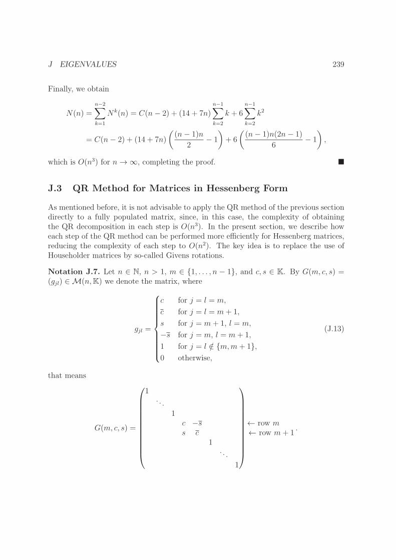
J EIGENVALUES 239
Finally, we obtain
N(n) =n−2∑
k=1
Nk(n) = C(n− 2) + (14 + 7n)n−1∑
k=2
k + 6n−1∑
k=2
k2
= C(n− 2) + (14 + 7n)
((n− 1)n
2− 1
)+ 6
((n− 1)n(2n− 1)
6− 1
),
which is O(n3) for n→∞, completing the proof. �
J.3 QR Method for Matrices in Hessenberg Form
As mentioned before, it is not advisable to apply the QR method of the previous sectiondirectly to a fully populated matrix, since, in this case, the complexity of obtainingthe QR decomposition in each step is O(n3). In the present section, we describe howeach step of the QR method can be performed more efficiently for Hessenberg matrices,reducing the complexity of each step to O(n2). The key idea is to replace the use ofHouseholder matrices by so-called Givens rotations.
Notation J.7. Let n ∈ N, n > 1, m ∈ {1, . . . , n − 1}, and c, s ∈ K. By G(m, c, s) =(gjl) ∈M(n,K) we denote the matrix, where
gjl =
c for j = l = m,
c for j = l = m+ 1,
s for j = m+ 1, l = m,
−s for j = m, l = m+ 1,
1 for j = l /∈ {m,m+ 1},0 otherwise,
(J.13)
that means
G(m, c, s) =
1. . .
1c −ss c
1. . .
1
← row m← row m+ 1
.
J EIGENVALUES 240
Lemma J.8. Let n ∈ N, n > 1, m ∈ {1, . . . , n − 1}, and c, s ∈ K. Let G(m, c, s) =(gjl) ∈M(n,K) be as in Not. J.7.
(a) If |c|2+ |s|2 = 1, then G(m, c, s) is unitary (in this case, G(m, c, s) is a special caseof what is known as a Givens rotation).
(b) If A = (ajl) ∈ M(n,K) is in Hessenberg form with a21 = · · · = am,m−1 = 0,am+1,m 6= 0,
c :=a√
|a|2 + |b|2, s :=
b√|a|2 + |b|2
, a := amm, b := am+1,m, (J.14)
and B = (bjl) := G(m, c, s)∗A, then B is still in Hessenberg form, but with b21 =· · · = bm,m−1 = bm+1,m = 0. Moreover, |c|2 + |s|2 = 1. Rows m + 2 through n areidentical in A and B.
Proof. (a): G(m, c, s) is unitary, since
(c −ss c
)(c s−s c
)=
(|c|2 + |s|2 cs− scsc− cs |c|2 + |s|2
)= Id,
implying G(m, c, s)G(m, c, s)∗ = Id.
(b): Clearly, |c|2 + |s|2 = 1. Due to the form of G(m, c, s)∗, G(m, c, s)∗A can onlyaffect rows m and m + 1 of A (all other rows are the same in A and B). As A is inHessenberg form with a21 = · · · = am,m−1 = 0, this further implies that columns 1through m− 1 are also the same in A and B, implying B to be in Hessenberg form withb21 = · · · = bm,m−1 = 0 as well. Finally,
bm+1,m = −s amm + c am+1,m =−ba+ ab√|a|2 + |b|2
= 0,
thereby establishing the case. �
The idea of each step of the QR method for matrices in Hessenberg form is to transformA(k) into A(k+1) by a sequence of n − 1 unitary similarity transformations via Givensrotations Gk1, . . . , Gk,n−1. The Gkm are chosen such that the sequence
A(k) =: A(k,1) 7→ A(k,2) := G∗k1A
(k,1)
7→ . . . 7→ Rk := A(k,n) := G∗k,n−1A
(k,n−1)
transforms A(k) into an upper triangular matrix Rk:
J EIGENVALUES 241
Lemma J.9. If A(k) ∈ M(n,K) is a matrix in Hessenberg form, n ∈ N, n ≥ 2,A(k,1) =: A(k), and, for each m ∈ {1, . . . , n− 1},
A(k,m+1) := G∗kmA
(k,m), (J.15)
Gkm = Id for a(k)m+1,m = 0, otherwise Gkm = G(m, c, s) with c, s defined as in (J.14),
except with a := a(k,m)mm and b := a
(k)m+1,m, then each A(k,m) is in Hessenberg form, a
(k,m)21 =
· · · = a(k,m)m,m−1 = 0, and rows m + 1 through n are identical in A(k,m) and in A(k). In
particular, Rk := A(k,n) is an upper triangular matrix.
Proof. This is just Lem. J.8(b) combined with a straightforward induction on m. �
Algorithm J.10 (QR Method for Matrices in Hessenberg Form). Given A ∈M(n,K)in Hessenberg form, n ∈ N, n ≥ 2, we define the following algorithm for the computationof a sequence (A(k))k∈N of matrices inM(n,K): Let A(1) := A. For each k ∈ N, A(k+1)
is obtained from A(k) by a sequence of n− 1 unitary similarity transformations:
A(k) =: B(k,1) 7→ B(k,2) := G∗k1B
(k,1)Gk1
7→ . . . 7→ A(k+1) := B(k,n) := G∗k,n−1B
(k,n−1)Gk,n−1, (J.16a)
where the Gkm, m ∈ {1, . . . , n − 1}, are defined as in Lem. J.9. To obtain Gkm, one
needs to know a(k,m)mm and a
(k)m+1,m. However, as it turns out, one does not actually have
to compute the matrices A(k,m) explicitly, since, letting
∀m∈{1,...,n−1}
C(k,m) := G∗kmB
(k,m), (J.16b)
one has (see Th. J.11(c) below)
∀m∈{1,...,n−2}
c(k,m)m+1,m+1 = a
(k,m+1)m+1,m+1, c
(k,m)m+2,m+1 = a
(k)m+2,m+1. (J.16c)
Thus, when computing B(k,m+1) for (J.16a), one computes C(k,m) first and stores theelements in (J.16c) to be available to obtain Gk,m+1.
Theorem J.11. Let A ∈ M(n,K) be in Hessenberg form, n ∈ N, n ≥ 2. Let thematrices A(k), A(k,m), B(k,m), and C(k,m) be defined as in Alg. J.10.
(a) The QR method for matrices in Hessenberg form as defined in Alg. J.10 is, indeed,a QR method as defined in Alg. 7.18, i.e. (7.37) holds for the A(k). In particular,Alg. J.10 preserves the eigenvalues (with multiplicities) of A and Th. 7.22 applies(also cf. Rem. 7.23(a)).

J EIGENVALUES 242
(b) Each C(k,m) and each A(k) is in Hessenberg form.
(c) Let m ∈ {1, . . . , n − 1}. Then all columns with indices m + 1 through n of thematrices C(k,m) and A(k,m+1) are identical (in particular, (J.16c) holds true).
Proof. Step 1: Assuming A(k) to be in Hessenberg form, we show that each C(k,m),m ∈ {1, . . . , n− 1}, is in Hessenberg form as well, (c) holds, and A(k+1) is in Hessenbergform: Let m ∈ {1, . . . , n− 1}. According to the definition in Lem. J.9,
A(k,m+1) = G∗km · · ·G∗
k1A(k).
Thus, according to (J.16a),
C(k,m) = G∗kmB
(k,m) = G∗kmG
∗k,m−1 · · ·G∗
k1A(k)Gk1 · · ·Gk,m−1
= A(k,m+1)Gk1 · · ·Gk,m−1. (J.17)
If a matrix Z ∈ M(n,K) is in Hessenberg form with zl+1,l = zl+2,l+1 = 0, then rightmultiplication by Gkl only affects columns l, l + 1 of Z and rows 1, . . . , l + 1 of Z. AsA(k,m+1) is in Hessenberg form with a
(k,m+1)21 = · · · = a
(k,m+1)m+1,m = 0 by Lem. J.9, (J.17)
implies C(k,m) is in Hessenberg form with columns m, . . . , n of C(k,m) and A(k,m+1) beingidentical. As A(k+1) = C(k,n−1)Gk,n−1, and Gk,n−1 only affects columns n − 1 and n ofC(k,n−1), A(k+1) must also be in Hessenberg form, concluding Step 1.
Step 2: Assuming A(k) to be in Hessenberg form, we show (7.37) to hold for A(k) andA(k+1): According to (J.16a),
A(k+1) = G∗k,n−1 · · ·G∗
k1A(k)Gk1 · · ·Gk,n−1 = RkQk, (J.18a)
where
Rk = G∗k,n−1 · · ·G∗
k1A(k), Qk := Gk1 · · ·Gk,n−1, A(k) = Qk Rk. (J.18b)
As Rk is upper triangular by Lem. J.9 and Qk is unitary (as it is the product of unitarymatrices), we have proved that (7.37) holds and, thereby, completed Step 2.
Finally, since A(1) is in Hessenberg form by hypothesis, using Steps 1 and 2 in aninduction on k concludes the proof of the theorem. �
Remark J.12. In the situation of Alg. J.10 it takes O(n2) arithmetic operations totransform A(k) into A(k+1) (see the proof of Th. J.6(c) for a list of admissible arithmeticoperations): One has to obtain the n− 1 Givens rotations Gk1, . . . , Gk,n−1 using (J.14),and one also needs the adjoint n−1 Givens rotations. As the number of nontrivial entriesin the Gkm is always 4 and, thus, independent of n, the total of arithmetic operations
K MINIMIZATION 243
to obtain the Gkm is NG(n) = O(n). Since each C(k,m) is in Hessenberg form, rightmultiplication with Gkm only affects at most an (m+2)× 2 submatrix, needing at mostC(m+2) arithmetic operations, C ∈ N. The result differs from a Hessenberg matrix atmost in one element, namely the element with index (m+ 2,m), i.e. left multiplicationof the result with G∗
k,m+1 only affects at most an 2× (n−m) submatrix, needing at mostC(n −m) arithmetic operations (this is also consistent with the very first step, whereone computes G∗
k1A(k) with A(k) in Hessenberg form). Thus, the total is at most
NG(n) + (n− 1)C(n−m+ 1 +m+ 2) = NG(n) + (n− 1)C(n+ 3),
which is O(n2) for n→∞.
K Minimization
K.1 Golden Section Search
The goal of this section is to provide a derivative-free algorithm for one-dimensionalminimization problems
min f(t), f : I −→ R, I ⊆ R, (K.1)
that is worst-case optimal in the same way the bisection method is worst-case optimal forroot-finding problems. Let us emphasize that one-dimensional minimization problemsalso often occur as subproblems, so-called line searches in multi-dimensional minimiza-tion: One might use a derivative-based method to determine a descent direction u atsome point x for some objective function J : X −→ R, that means some u ∈ X suchthat the auxiliary objective function
f : [0, a[−→ R, f(t) := J(x+ tu) (K.2)
is known to be decreasing in some neighborhood of 0. The line search then aims tominimize J on the line segment {x+tu : t ∈ [0, a[}, i.e. to perform the (one-dimensional)minimization of f .
Recall the bisection algorithm for finding a zero of a one-dimensional continuous functionf : [a, b] −→ R, defined on some interval [a, b] ⊆ R, a < b, with f(a) < 0 < f(b): In eachstep, one has an interval [an, bn], an < bn, with f(an) < 0 < f(bn), and one evaluatesf at the midpoint cn := (an + bn)/2, choosing [an, cn] as the next interval if f(cn) > 0and [cn, bn] if f(cn) < 0. If f is continuous, then the boundary points of the intervalsconverge to a zero of f . Choosing the midpoint is worst-case optimal in the sense that,without further knowledge on f , any other choice for cn might force one to choose the

K MINIMIZATION 244
larger of the two subintervals for the next step, which would then have length biggerthan (bn − an)/2.As we will see below, golden section search is the analogue of the bisection algorithmfor minimization problems, where the situation is slightly more subtle. First, we haveto address the problem of bracketing a minimum: For the bisection method, by theintermediate value theorem, a zero of the continuous function f is bracketed if f(a) <f(b) (or f(a) > f(b)). However, to bracket the min of a continuous function f , we needthree points a < b < c, where
f(b) = min{f(a), f(b), f(c)}. (K.3)
Definition K.1. Let I ⊆ R be an interval, f : I −→ R. Then (a, b, c) ∈ I3 is called aminimization triplet for f if, and only if, a < b < c and (K.3) holds.
—
Clearly, if f is continuous, then (K.3) implies f to have (at least one) global min in ]a, b[.Thus, the problem of bracketing a minimum is to determine a minimization triplet forf , where one has to be aware that the problem has no solution if f is strictly increasingor strictly decreasing. Still, we can formulate the following algorithm:
Algorithm K.2 (Bracketing a Minimum). Let f : I −→ R be defined on a nontrivialinterval I ⊆ R, m := inf I, M := sup I. We define a finite sequence (a1, a2, . . . , aN),N ≥ 3, of distinct points in I via the following recursion: For the first two points choosea < b in the interior of I. Set
a1 := a, a2 := b, σ := 1 if f(b) ≤ f(a),
a1 := b, a2 := a, σ := −1 if f(b) > f(a).(K.4)
If the algorithm has not been stopped in the pevious step (i.e. if 2 ≤ n < N), then settn := an + 2σ|an − an−1| and
an+1 :=
tn if tn ∈ I,M if tn > M , M ∈ I,(an +M)/2 if tn > M , M /∈ I,m if tn < m, m ∈ I,(m+ an)/2 if tn < m, m /∈ I.
(K.5)
Stop the iteration (and set N := n + 1) if at least one of the following conditionsis satisfied: (i) f(an+1) ≥ f(an), (ii) an+1 ∈ {m,M}, (iii) an+1 /∈ [amin, amax] (whereamin, amax ∈ I are some given bounds), (iv) n+1 = nmax (where nmax ∈ N is some givenbound).

K MINIMIZATION 245
Remark K.3. (a) Since (K.4) guarantees f(a1) ≥ f(a2), condition (i) plus an induc-tion shows
f(a1) ≥ f(a2) > · · · > f(aN−1).
(b) If Alg. K.2 terminates due to condition (i), then (a) implies (aN−2, aN−1, aN) (forσ = 1) or (aN , aN−1, aN−2) (for σ = −1) to be a minimization triplet for f .
(c) If Alg. K.2 terminates due to conditions (ii) – (iv) (and (i) is not satisfied), then themethod has failed to find a minimization triplet for f . One then has three options:(a) abort the search (after all, a minimization triplet for f might not exist and aNis a good candidate for a local min), (b) search on the other side of a1, (c) continuethe original search with adjusted bounds (if possible).
—
Given a minimization triplet (a, b, c) for some function f , we now want to evaluate f atx ∈]a, b[ or at x ∈]b, c[ to obain a new minimization triplet (a′, b′, c′), where c′−a′ < c−a.Moreover, the strategy for choosing x should be worst-case optimal.
Lemma K.4. Let I ⊆ R be an interval, f : I −→ R. If (a, b, c) ∈ I3 is a minimizationtriplet for f , then so are the following triples:
(a, x, b) for a < x < b and f(b) ≥ f(x), (K.6a)
(x, b, c) for a < x < b and f(b) ≤ f(x), (K.6b)
(a, b, x) for b < x < c and f(b) ≤ f(x), (K.6c)
(b, x, c) for b < x < c and f(b) ≥ f(x). (K.6d)
Proof. All four cases are immediate. �
While Lem. K.4 shows the forming of new, smaller triplets to be easy, the questionremains of how to choose x. Given a minimization triplet (a, b, c), the location of b is afraction w of the way between a and c, i.e.
w :=b− ac− a, 1− w =
c− bc− a. (K.7)
We will now assume w ≤ 12– if w > 1
2, then one can make the analogous (symmetric)
argument, starting from c rather than from a (we will come back to this point below).The new point x will be an additional fraction z toward c,
z :=x− bc− a . (K.8)

K MINIMIZATION 246
If one chooses the new minimization triplet according to (K.6), then its length l is
l =
w (c− a) for a < x < b and f(b) ≥ f(x),
(1− (w + z)) (c− a) for a < x < b and f(b) ≤ f(x),
(w + z) (c− a) for b < x < c and f(b) ≤ f(x),
(1− w) (c− a) for b < x < c and f(b) ≥ f(x).
(K.9)
For the moment, consider the case b < x < c. As we assume no prior knowledge aboutf , we have no control over which of the two choices we will have to make to obtain thenew minimization triplet, i.e., if possible, we should make the last two factors in frontof c− a in (K.9) equal, leading to w + z = 1− w or
z = 1− 2w. (K.10)
If we were to choose x between a and b, then it could occur that l = (1−(w+z)) > 1−w(note z < 0 in this case), that means this choice is not worst-case optimal. Togetherwith the symmetric argument for w > 1
2, this means we always need to put x in the
larger of the two subintervals. While (K.10) provides a formula for determining z interms of w, we still have the freedom to choose w. If there is an optimal value for w,then this value should remain constant throughout the algorithm – it should be thesame for the old triplet and for the new triplet. This leads to
w =x− bc− b
(K.8)=
z(c− a)c− b
(K.7)=
z
1− w, (K.11)
which, combined with (K.10), yields
w2 − 3w + 1 = 0 ⇔ w =3±√5
2. (K.12)
Fortunately, precisely one of the values of w in (K.12) satisfies 0 < w < 12, namely
w =3−√5
2≈ 0.38, 1− w =
√5− 1
2≈ 0.62. (K.13)
Then 1−ww
= 1+√5
2is the value of the golden ratio or golden section, which gives the
following Alg. K.5 its name. Together with the symmetric argument for w > 12, we can
summarize our findings by stating that the new point x should be a fraction of w = 3−√5
2
into the larger of the two subintervals (where the fraction is measured from the centralpoint of the triplet):

K MINIMIZATION 247
Algorithm K.5 (Golden Section Search). Let I ⊆ R be a nontrivial interval, f : I −→R. Assume that (a, b, c) ∈ I3 is a minimization triplet for f . We define the followingrecursive algorithm for the computation of a sequence of minimization triplets for f :Set (a1, b1, c1) := (a, b, c). Given n ∈ N and a minimization triplet (an, bn, cn), set
xn :=
{bn + w(cn − bn) if cn − bn ≥ bn − an,bn − w(bn − an) if cn − bn < bn − an,
w :=3−√5
2, (K.14)
and choose (an+1, bn+1, cn+1) according to (K.6) (in practise, one will stop the iterationif cn − an < ǫ, where ǫ > 0 is some given bound).
Lemma K.6. Consider Alg. K.5.
(a) The value of f(bn) decreases monotonically, i.e. f(bn+1) ≤ f(bn) for each n ∈ N.
(b) With the possible exception of one step, one always has
cn+1 − an+1 ≤ q (cn − an), where q :=1
2+α
2≈ 0.69, α :=
3−√5
2. (K.15)
(c) One has
x := limn→∞
an = limn→∞
bn = limn→∞
cn, {x} =⋂
n∈N[an, cn]. (K.16)
Proof. (a) clearly holds, since each new minimization triplet is chosen according to(K.6).
(b): As, according to (K.14), xn is always chosen in the larger subinterval, it suffices toconsider the case w := bn−an
cn−an≤ 1
2. If w = α, then (K.9) and (K.10) guarantee
cn+1 − an+1 = (w + z)(cn − an) = (1− w)(cn − an) < q(cn − an).
Moreover, due to (K.11), if w = α (or w = 1 − α) has occurred once, then w = α orw = 1 − α will hold for all following steps. Let w 6= α, w ≤ 1
2. If (an+1, bn+1, cn+1) =
(bn, xn, cn), then (K.15) might not hold, but w = α holds in the next step, i.e. (K.15) doeshold for all following steps. Thus, it only remains to consider the case (an+1, bn+1, cn+1)= (an, bn, xn). In this case,
cn+1 − an+1
cn − an=xn − ancn − an
=bn − ancn − an
+xn − bncn − an
= w +xn − bncn − bn
cn − bncn − an
= w + α(1− w) = α + (1− α)w ≤ α + (1− α)12= q,

K MINIMIZATION 248
establishing the case.
(c): Clearly, [an+1, cn+1] ⊆ [an, cn] for each n ∈ N. Applying an induction to (K.15)yields
∀n∈N
cn+1 − an+1 ≤ qn−1(c1 − a1),
where the exponent on the right-hand side is n − 1 instead of n due to the possibleexception in one step. Since q < 1, this means limn→∞(cn−an) = 0, proving (K.16). �
Definition K.7. Let I ⊆ R be an interval, f : I −→ R. We call f locally monotoneif, and only if, for each x ∈ I, there exists ǫ > 0 such that f is monotone (increasing ordecreasing) on I∩]x− ǫ, x] and monotone on I ∩ [x, x+ ǫ[.
Example K.8. The function
f : R −→ R, f(x) :=
{x sin 1
xfor x 6= 0,
0 for x = 0,
is an example of a continuous function that is not locally monotone (clearly, f is notmonotone in any interval ]− ǫ, 0] or [0, ǫ[, ǫ > 0).
Theorem K.9. Let I ⊆ R be a nontrivial interval and assume f : I −→ R to becontinuous and locally monotone in the sense of Def. K.7. Consider Alg. K.5 and letx := limn→∞ bn (cf. Lem. K.6(c)). Then f has a local min at x.
Proof. The continuity of f implies f(x) = limn→∞ f(bn). Then Lem. K.6(a) implies
f(x) = inf{f(bn) : n ∈ N}. (K.17)
If f does not have a local min at x, then
∀n∈N
∃yn∈I
(yn ∈]an, cn[ and f(yn) < f(x)
). (K.18)
If an < yn < x, then f(an) > f(yn) < f(x), showing f is not monotone in [an, x].Likewise, if x < yn < cn, then f(x) > f(yn) < f(cn), showing f is not monotonein [x, cn]. Thus, there is no ǫ > 0 such that f is monotone on both I∩]x − ǫ, x] andI ∩ [x, x+ ǫ[, in contradiction to the assumption that f be locally monotone. �
K.2 Nelder-Mead Method
The Nelder-Mead method of [NM65] is a method for minimization in Rn, i.e. for anobjective function f : Rn −→ R. It is also known as the downhill simplex method or

K MINIMIZATION 249
the amoeba method. The method has nothing to do with the simplex method of linearprogramming (execpt that both methods make use of the geometrical structure calledsimplex).
The Nelder-Mead method is a derivative-free method that is simple to implement. Itis an example of a method that seems to perform quite well in practise, even thoughthere are known examples, where it will fail, and, in general, the related convergencetheory available in the literature remains quite limited. Here, we will merely presentthe algorithm together with its heuristics, and provide some relevant references to theliterature.
Recall that a (nondegenerate) simplex in Rn is the convex hull of n+1 points x1, . . . , xn+1
∈ Rn such that the points x2 − x1, . . . , xn+1 − x1 are linearly independent. If ∆ =conv{x1, . . . , xn+1}, then x1, . . . , xn+1 are called the vertices of ∆.
The idea of the Nelder-Mead method is to construct a sequence (∆k)k∈N,
∆k = conv{xk1, . . . , xkn+1} ⊆ Rn, (K.19)
of simplices such that the size of the ∆k converges to 0 and the value of f at the verticesof the ∆k decreases, at least on average. To this end, in each step, one finds the vertexv, where f is largest and either replaces v by a new vertex (by moving it in the directionof the centroid of the remaining vertices, see below) or one shrinks the simplex.
Algorithm K.10 (Nelder-Mead). Given f : Rn −→ R, n ∈ N, we provide a recursionto obtain a sequence of simplices (∆k)k∈N as in (K.19):
Initialization: Choose x11 ∈ Rn \ {e1, . . . , en} (the initial guess for the desired min of f),and set
∀i∈{1,...,n}
x1i+1 := x11 + δi ei, (K.20)
where the ei denote the standard unit vectors, and the δi > 0 are initialization param-eters that one should try to adapt to the (conjectured) characteristic length scale (orscales) of the considered problem.
Iteration Step: Given ∆k, k ∈ N, sort the vertices such that (K.19) holds with
f(xk1) ≤ f(xk2) · · · ≤ f(xkn+1). (K.21)
According to the following rules, we will either replace (only) xkn+1 or shrink the simplex.In preparation, we compute the centroid of the first n vertices, i.e.
x :=1
n
n∑
i=1
xki , (K.22a)

K MINIMIZATION 250
and the search direction u for the new vertex,
u := x− xkn+1. (K.22b)
One will now apply precisely one of the following rules (1) – (4) in decreasing priority(i.e. rule (j) can only be used if none of the conditions for rules (1) – (j − 1) applied):
(1) Reflection: Compute the reflected point
xr := x+ µr u = xkn+1 + (µr + 1) u (K.23a)
and the corresponding valuefr := f(xr), (K.23b)
where µr > 0 is the reflection parameter (µr = 1 being a common setting). If
f(xk1) ≤ fr < f(xkn), (K.23c)
then replace xkn+1 with xr to obtain the new simplex ∆k+1. Heuristics: As f is largestat xkn+1, one reflects the point through the hyperplane spanned by the remainingvertices hoping to find smaller values on the other side. If one, indeed, finds asufficiently smaller value (better than the second worst), then one takes the newpoint, except if the new point has a smaller value than all other vertices, in whichcase, one tries to go even further in that direction by applying rule (2) below.
(2) Expansion: Iff(xr) < f(xk1) (K.24a)
(i.e. (K.23c) does not hold and xr is better than all xki ), then compute the expandedpoint
xe := x+ µe u = xkn+1 + (µe + 1) u, (K.24b)
where µe > µr is the expansion parameter (µe = 2 being a common setting). If
f(xe) < fr, (K.24c)
then replace xkn+1 with xe to obtain the new simplex ∆k+1. If (K.24c) does not hold,then, as in (1), replace xkn+1 with xr to obtain ∆k+1. If neither (K.23c) nor (K.24a)holds, then continue with (3) below. Heuristics: If xr has the smallest value so far,then one hopes to find even smaller values by going further in the same direction.
(3) Contraction: If neither (K.23c) nor (K.24a) holds, then
fr ≥ f(xkn). (K.25a)

K MINIMIZATION 251
In this cases, compute the contracted point
xc := x+ µc u = xkn+1 + (µc + 1) u, (K.25b)
where −1 < µc < 0 is the contraction parameter (µc = −12being a common setting).
Iff(xc) < f(xkn+1), (K.25c)
then replace xkn+1 with xc to obtain the new simplex ∆k+1. Heuristics: If (K.25a)holds, then xr would still be the worst vertex of the new simplex. If the new vertexis to be still the worst, then it should at least be such that it reduces the volume ofthe simplex. Thus, the contracted point is chosen between xkn+1 and x.
(4) Reduction: If (K.25a) holds and (K.25c) does not hold, then we have failed to find abetter vertex in the direction u. We then shrink the simplex around the best pointxk1 by setting xk+1
1 := xk1 and
∀i∈{2,...,n+1}
xk+1i := xk1 + µs (x
ki − xk1), (K.26)
where 0 < µs < 1 is the shrink parameter (µs = 12being a common setting).
Heuristics: If f increases by moving from the worst point in the direction of thebetter points, then that indicates the simplex being too large, possibly containingseveral local mins. Thus, we shrink the simplex around the best point, hoping tothereby improve the situation.
Remark K.11. Consider Alg. K.10.
(a) Clearly, all simplices ∆k, k ∈ N, are nondegenerate: For ∆1 this is guaranteed bychoosing x11 /∈ {e1, . . . , en}; for k > 1, this is guaranteed since (1) – (3) choosethe new vertex not in conv{xk1, . . . , xkn} (note {xkn+1 + µ(x − xkn+1) : µ ∈ R} ∩conv{xk1, . . . , xkn} = {x}), and xk2 − xk1, . . . , x
kn+1 − xk1 are linearly independent in
(4).
(b) (1) – (3) are designed such that the average value of f at the vertices decreases:
1
n+ 1
n+1∑
i=1
f(xk+1i ) <
1
n+ 1
n+1∑
i=1
f(xki ). (K.27)
However, if (4) occurs, then (K.27) can fail to hold.
(c) As mentioned above, even though Alg. K.10 seems to perform well in practise, onecan construct examples, where it will converge to points that are not local minima

REFERENCES 252
(see, e.g., [Kel99, Sec. 8.1.3]). Some positive results regarding the convergence ofAlg. K.10 can be found in [Kel99, Sec. 8.1.2] and [LRWW98]. In general, multidi-mensional minimization is not an easy task, and it is not uncommon for algorithmsto converge to wrong points. It is therefore recommended in [PTVF07, pp. 503-504]to restart the algorithm at a point that it claimed to be a minimum (also see [Kel99,Sec. 8.1.4] regarding restarts of Alg. K.10).
References
[Alt06] Hans Wilhelm Alt. Lineare Funktionalanalysis, 5th ed. Springer-Verlag,Berlin, 2006 (German).
[Blu68] L.I. Bluestein. A linear filtering approach to the computation of the dis-crete Fourier transform. Northeast Electronics Research and EngineeringMeeting Record 10 (1968), 218–219.
[Bos13] Siegfried Bosch. Algebra, 8th ed. Springer-Verlag, Berlin, 2013 (Ger-man).
[Bra77] Helmut Brass. Quadraturverfahren. Studia Mathematica, Vol. 3, Van-denhoeck & Ruprecht, Gottingen, Germany, 1977, in German.
[Cia89] Philippe G. Ciarlet. Introduction to numerical linear algebra and opti-mization. Cambridge Texts in Applied Mathematics, Cambridge UniversityPress, Cambridge, UK, 1989.
[Deu11] Peter Deuflhard. Newton Methods for Nonlinear Problems. SpringerSeries in Computational Mathematics, Vol. 35, Springer, Berlin, Germany,2011.
[DH08] Peter Deuflhard and Andreas Hohmann. Numerische Mathematik1, 4th ed. Walter de Gruyter, Berlin, Germany, 2008 (German).
[FH07] Roland W. Freund and Ronald H.W. Hoppe. Stoer/Bulirsch: Nu-merische Mathematik 1, 10th ed. Springer, Berlin, Germany, 2007 (Ger-man).
[GK99] Carl Geiger and Christian Kanzow. Numerische Verfahren zurLosung unrestringierter Optimierungsaufgaben. Springer-Verlag, Berlin,Germany, 1999 (German).
REFERENCES 253
[HB09] Martin Hanke-Bourgeois. Grundlagen der Numerischen Mathematikund des Wissenschaftlichen Rechnens, 3rd ed. Vieweg+Teubner, Wies-baden, Germany, 2009 (German).
[Heu08] Harro Heuser. Lehrbuch der Analysis Teil 2, 14th ed. Vieweg+Teubner,Wiesbaden, Germany, 2008 (German).
[HH92] G. Hammerlin and K.-H. Hoffmann. Numerische Mathematik, 3rd ed.Grundwissen Mathematik, Vol. 7, Springer-Verlag, Berlin, 1992 (German).
[Kel99] C.T. Kelley. Iterative Methods for Optimization. SIAM, Philadelphia,USA, 1999.
[LRWW98] J.C. Lagarias, J.A. Reeds, M.H. Wright, and P.E. Wright. Con-vergence Properties of the Nelder-Mead Simplex Method in Low Dimensions.SIAM J. Optim. 9 (1998), No. 1, 112–147.
[NM65] J.A. Nelder and R. Mead. A simplex method for function minimization.Comput. J. 7 (1965), 308–313.
[OR70] J.M. Ortega and W.C. Rheinboldt. Iterative Solution of NonlinearEquations in Several Variables. Computer Science and Applied Mathemat-ics, Academic Press, New York, 1970.
[Phi09] P. Philip. Optimal Control of Partial Differential Equations. LectureNotes, Ludwig-Maximilians-Universitat, Germany, 2009, available in PDFformat at http://www.math.lmu.de/~philip/publications/lectureNot
es/philipPeter_OptimalControlOfPDE.pdf.
[Phi16a] P. Philip. Analysis I: Calculus of One Real Variable. Lecture Notes, LMUMunich, 2015/2016, AMS Open Math Notes Ref. # OMN:202109.111306,available in PDF format athttps://www.ams.org/open-math-notes/omn-view-listing?listingId=111306.
[Phi16b] P. Philip. Analysis II: Topology and Differential Calculus of Several Vari-ables. Lecture Notes, LMU Munich, 2016, AMS Open Math Notes Ref. #OMN:202109.111307, available in PDF format athttps://www.ams.org/open-math-notes/omn-view-listing?listingId=111307.
[Phi16c] P. Philip. Ordinary Differential Equations. Lecture Notes, Ludwig-Maximilians-Universitat, Germany, 2016, available in PDF format athttp://www.math.lmu.de/~philip/publications/lectureNotes/philipPeter_ODE.pdf.

REFERENCES 254
[Phi17] P. Philip. Analysis III: Measure and Integration Theory of Several Vari-ables. Lecture Notes, LMU Munich, 2016/2017, AMS Open Math NotesRef. # OMN:202109.111308, available in PDF format athttps://www.ams.org/open-math-notes/omn-view-listing?listingId=111308.
[Phi19a] P. Philip. Linear Algebra I. Lecture Notes, Ludwig-Maximilians-Universitat, Germany, 2018/2019, AMS Open Math Notes Ref. #OMN:202109.111304, available in PDF format athttps://www.ams.org/open-math-notes/omn-view-listing?listingId=111304.
[Phi19b] P. Philip. Linear Algebra II. Lecture Notes, Ludwig-Maximilians-Univer-sitat, Germany, 2019, AMS Open Math Notes Ref. # OMN:202109.111305,available in PDF format athttps://www.ams.org/open-math-notes/omn-view-listing?listingId=111305.
[Pla10] Robert Plato. Numerische Mathematik kompakt, 4th ed. Vieweg Verlag,Wiesbaden, Germany, 2010 (German).
[PTVF07] W.H. Press, S.A. Teukolsky, W.T. Vetterling, and B.P. Flan-
nery. Numerical Recipes. The Art of Scientific Computing, 3rd ed. Cam-bridge University Press, New York, USA, 2007.
[QSS07] Alfio Quarteroni, Riccardo Sacco, and Fausto Saleri. NumericalMathematics, 2nd ed. Texts in Applied Mathematics, Vol. 37, Springer-Verlag, Berlin, 2007.
[RSR69] L.R. Rabiner, R.W. Schafer, andC.M. Rader. The chirp z-transformalgorithm and its application. Bell Syst. Tech. J. 48 (1969), 1249–1292.
[Rud87] W. Rudin. Real and Complex Analysis, 3rd ed. McGraw-Hill Book Com-pany, New York, 1987.
[Sco11] L. Ridgway Scott. Numerical Analysis. Princeton University Press,Princeton, USA, 2011.
[SK11] H.R. Schwarz and N. Kockler. Numerische Mathematik, 8th ed.Vieweg+Teubner Verlag, Wiesbaden, 2011 (German).
[Str08] Gernot Stroth. Lineare Algebra, 2nd ed. Berliner Studienreihe zurMathematik, Vol. 7, Heldermann Verlag, Lemgo, Germany, 2008 (German).
[SV01] J. Saranen and G. Vainikko. Periodic Integral and PseudodifferentialEquations with Numerical Approximation. Springer, Berlin, 2001.

REFERENCES 255
[Wer11] D. Werner. Funktionalanalysis, 7th ed. Springer-Verlag, Berlin, 2011(German).
[Yos80] K. Yosida. Functional Analysis, 6th ed. Grundlehren der mathematischenWissenschaften, Vol. 123, Springer-Verlag, Berlin, 1980.