numerical validation and refinement of empirical rock mass modulus
TRANSCRIPT

8/11/2019 Numerical Validation and Refinement of Empirical Rock Mass Modulus
http://slidepdf.com/reader/full/numerical-validation-and-refinement-of-empirical-rock-mass-modulus 1/263
NUMERICAL VALIDATION AND REFINEMENT OF EMPIRICAL
ROCK MASS MODULUS ESTIMATION
by
Colin David Hume
A thesis submitted to the Department of Geological Sciences & Geological Engineering
In conformity with the requirements for
the degree of Master of Science

8/11/2019 Numerical Validation and Refinement of Empirical Rock Mass Modulus
http://slidepdf.com/reader/full/numerical-validation-and-refinement-of-empirical-rock-mass-modulus 2/263
Abstract
A sound understanding of rock mass characteristics is critical for the engineering prediction of
tunnel stability and deformation both during construction and post-excavation. The rock mass
modulus of deformation is a necessary input parameter for many numerical analysis methods to
describe the constitutive behavior of a rock mass. Tests for determining this parameter directly by
in situ test methods are inherently difficult, time consuming and expensive, and these challenges
are more problematic when dealing with tunnels in weaker, softer rock masses where errors in
modulus (stiffness) estimation have a profound impact on closure predictions. In addition, rock
masses with modest structure can be candidate sites for highly sensitive structures such as nuclear
waste repository tunnels. For these generally stiffer rock masses, the correct modulus assessment
is essential for prediction of thermal response during the service life of the tunnel.
Numerous empirical relationships based on rock mass classification schemes have been
developed to determine rock mass deformation modulus in response to these issues. The
empirical relationship provided by Hoek & Diederichs (2006) based on Geological Strength
Index (GSI) has been determined from a database of in situ test data describing a wide range of
k i h GSI l h 25 d l h 80 Wi hi hi f li i

8/11/2019 Numerical Validation and Refinement of Empirical Rock Mass Modulus
http://slidepdf.com/reader/full/numerical-validation-and-refinement-of-empirical-rock-mass-modulus 3/263
Acknowledgements
This work has been made possible through the financial contributions of the Natural Sciences and
Research Council of Canada (NSERC). I would also like to acknowledge the department of
Geological Sciences and Geological Engineering at Queen’s University, which has also provided
financial support towards the completion of this research.
My most sincere appreciation goes to my thesis advisor, Dr. Mark Diederichs for his inspiration
and full commitment to this work, and having a big hand in furthering my academic and
professional career.
I would like to acknowledge the help and support of my friends and colleagues Matt Lato, Matt
Perras and Ehsan Ghazvinian, as well as everyone else in our Geomechanics group. A special
thanks to Dr. Jean Hutchinson who has always been very helpful and for having mentioned this
opportunity to me initially.
I owe great thanks to my parents Bill and Judy Hume for their support and encouragement in all
aspects of my life regardless of what path I have chosen.
The immense love and support of my incredible wife Kathy Kalenchuk has been significant to the
l i f hi MS O li l Sh ld h h j h i

8/11/2019 Numerical Validation and Refinement of Empirical Rock Mass Modulus
http://slidepdf.com/reader/full/numerical-validation-and-refinement-of-empirical-rock-mass-modulus 4/263
Table of Contents
Abstract ............................................................................................................................................ ii
Acknowledgements ......................................................................................................................... iii
List of Symbols and Acronyms ................................................................................................... xviii
Chapter 1 Introduction ..................................................................................................................... 1
1.1 Background ............................................................................................................................ 1
1.1.1 Rock Mass Classification ................................................................................................ 2
1.1.2 Estimation of the Rock Mass Modulus of Deformation (Erm) ........................................ 3
1.2 Research Objectives ............................................................................................................... 5
1.2.1 Numerical Assessments of the Hoek-Diederichs Empirical Rock Mass Modulus of
Deformation Formula ............................................................................................................... 5
1.2.2 FEM Numerical Model Representation of GSI Rock Mass Classification System ........ 7
1.2.3 Joint Input Parameter Calibration from Block Models ................................................... 8
1.3 Summary of Findings ............................................................................................................. 8
1.4 Thesis Structure ..................................................................................................................... 9
1.5 References ............................................................................................................................ 11
Chapter 2 Rock Mass Classification Systems and their Application to Numerical Analysis ........ 13
2.1 Rock Mass Classification Systems ...................................................................................... 13
2.1.1 General .......................................................................................................................... 13
2.1.2 Rock Quality Designation (RQD) ................................................................................. 14
2 1 3 Rock Mass Rating System (RMR) 16

8/11/2019 Numerical Validation and Refinement of Empirical Rock Mass Modulus
http://slidepdf.com/reader/full/numerical-validation-and-refinement-of-empirical-rock-mass-modulus 5/263
2.1.6.2 Application and Limitations ................................................................................... 35
2.1.6.3 GSI Input Parameter Quantification ...................................................................... 36
2.2 Strength and Stiffness Parameter Estimation Methods Related to Tunnel Convergence .... 39
2.2.1 Generalized Hoek-Brown (GHB) Strength Criterion Parameters from GSI ................. 40
2.2.1.1 Disturbance Factor D ............................................................................................. 40
2.2.2 Erm Estimation ............................................................................................................... 40
2.2.3 Analytical Solutions to Problems in Rock Mechanics .................................................. 41
2.2.3.1 Circular Opening in an Infinite Elastic Medium .................................................... 41
2.2.3.2 Circular Opening in Inelastic Material ................................................................... 43
2.2.3.3 Ground Reaction Curve ......................................................................................... 44
2.3 Problem Statement ............................................................................................................... 45
2.4 References ............................................................................................................................ 46
Chapter 3 The Finite Element Method in Numerical Analysis ...................................................... 49
3.1 Background .......................................................................................................................... 49
3.2 Methodology ........................................................................................................................ 49
3.2.1 Elasticity Models .......................................................................................................... 51
3.2.2 Plasticity Models ........................................................................................................... 52
3.2.3 Discontinuity Representation in FEM ........................................................................... 55
3.2.3.1 General ................................................................................................................... 55
3.2.3.2 Joint Stiffness ......................................................................................................... 55
3.2.3.3 Joint Strength ......................................................................................................... 58
3 3 T l Ad M d lli i Pl S i FEM 62

8/11/2019 Numerical Validation and Refinement of Empirical Rock Mass Modulus
http://slidepdf.com/reader/full/numerical-validation-and-refinement-of-empirical-rock-mass-modulus 6/263
4.2.2 Isotropy and Anisotropy ............................................................................................... 74
4.3 Numerical Model Representation of the Modelling GSI Spectrum ..................................... 74
4.3.1 Rock Mass Structure ..................................................................................................... 74
4.4 Modelling Input Parameters ................................................................................................. 76
4.4.1 Stiffness Parameters ...................................................................................................... 77
4.4.1.1 Intact Rock ............................................................................................................. 77
4.4.1.2 Discontinuities ....................................................................................................... 78
4.4.1.3 Equivalent Rock Mass as a Continuum ................................................................. 83
4.4.2 Strength Parameters ...................................................................................................... 84
4.4.2.1 Intact Rock Parameters .......................................................................................... 84
4.4.2.2 Strength of Discontinuities..................................................................................... 85
4.4.2.3 Equivalent Rock Mass as a Continuum ................................................................. 88
4.5 Block Models ....................................................................................................................... 88
4.5.1 General .......................................................................................................................... 88
4.5.2 Boundary Conditions .................................................................................................... 89
4.5.2.1 External Boundaries ............................................................................................... 91
4.5.3 Joints ............................................................................................................................. 92
4.5.4 Sensitivity Analysis ...................................................................................................... 92
4.5.4.1 Scale Sensitivity ..................................................................................................... 92
4.5.4.2 Loading Method ..................................................................................................... 94
4.5.4.3 Initial Joint Deformation ........................................................................................ 95
4 5 4 4 O i i f J i 95

8/11/2019 Numerical Validation and Refinement of Empirical Rock Mass Modulus
http://slidepdf.com/reader/full/numerical-validation-and-refinement-of-empirical-rock-mass-modulus 7/263
Chapter 5 Results of Block Models ............................................................................................. 104
5.1 Introduction ........................................................................................................................ 104
5.2 Sensitivity Analysis ........................................................................................................... 105
5.2.1 Scale Sensitivity .......................................................................................................... 105
5.2.2 Loading Method .......................................................................................................... 108
5.2.3 Joint Orientation .......................................................................................................... 109
5.3 Final Analysis .................................................................................................................... 112
5.3.1 "Intact" Joint Structure (Models A1, A2 and A3) ....................................................... 114
5.3.2 "Blocky" Joint Structure (Models B1, B2, B3, B4 and B5) ........................................ 116
5.3.3 "Very Blocky" Joint Structure (Models C1, C2, C3, C4 and C5) ............................... 119
5.3.4 "Blocky/Disturbed/Seamy" Joint Structure (Models D1, D2, D3, D4 and D5) .......... 122
5.4 Discussion of Results ......................................................................................................... 124
5.4.1 General Observations .................................................................................................. 124
5.4.2 Results in Higher Quality Rock Mass (Greater than GSI 70) ..................................... 125
5.4.3 Results in Poorer Quality Rock Masses (less than GSI 35) ........................................ 126
5.5 References .......................................................................................................................... 128
Chapter 6 Results of Tunnel Models............................................................................................ 129
6.1 Introduction ........................................................................................................................ 129
6.2 Sensitivity Analysis ........................................................................................................... 129
6.2.1 Size of Jointed Rock Mass .......................................................................................... 129
6.2.2 Width of Representative Boundary ............................................................................. 131
6 2 3 M d l S 132

8/11/2019 Numerical Validation and Refinement of Empirical Rock Mass Modulus
http://slidepdf.com/reader/full/numerical-validation-and-refinement-of-empirical-rock-mass-modulus 8/263
6.4 Discussion of Results ......................................................................................................... 145
6.4.1 Higher Quality Rock Masses (GSI > 55) .................................................................... 145
6.4.2 Medium Quality Rock Masses (GSI 35-45)................................................................ 146
6.4.3 Poor Quality Rock Masses (GSI < 35) ........................................................................ 147
6.5 Conclusion ......................................................................................................................... 149
6.6 References .......................................................................................................................... 150
Chapter 7 Discussions and Conclusions ...................................................................................... 151
7.1 Summary of Findings ......................................................................................................... 151
7.2 Discussion .......................................................................................................................... 152
7.2.1 Representative Behaviour of Erm in FEM Analysis .................................................... 152
7.2.2 Proposed Corrections for Generalized Hoek-Diederichs for Tunnelling Applications
............................................................................................................................................. 153
7.3 Recommendations for Future Work ................................................................................... 162
7.4 Conclusion ......................................................................................................................... 163
7.5 References .......................................................................................................................... 163
Appendix A FEM Model Interpret Automation .......................................................................... 164
A.1 Overview ........................................................................................................................... 164
A.2 Comparisons of Block Model Values Interpolated using the Macro Versus Values
Extracted from Phase2 Interpret ............................................................................................... 164
A.3 Comparisons of Tunnel Model Values Interpolated using the Macro Versus Values
Extracted from Phase2 Interpret ............................................................................................... 166
A di B Di l S d h M C d 169

8/11/2019 Numerical Validation and Refinement of Empirical Rock Mass Modulus
http://slidepdf.com/reader/full/numerical-validation-and-refinement-of-empirical-rock-mass-modulus 9/263
List of Tables
Table 2-1: RMR 76 and RMR 89 Classification Parameters and Ratings after Bieniawski (1976,
1989) and Hoek et al. (1995) ......................................................................................................... 18
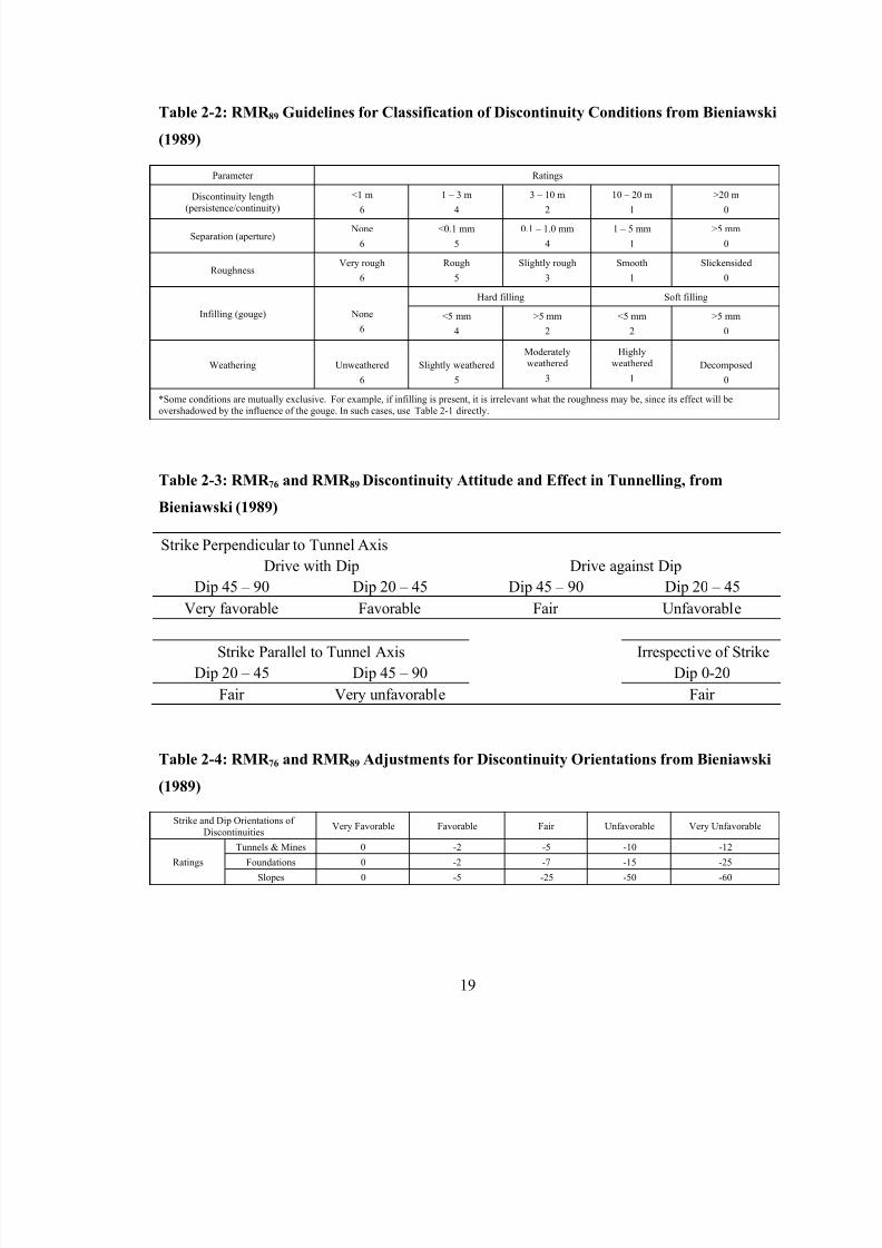
Table 2-2: RMR 89 Guidelines for Classification of Discontinuity Conditions from Bieniawski
(1989) ............................................................................................................................................. 19
Table 2-3: RMR 76 and RMR 89 Discontinuity Attitude and Effect in Tunnelling, from Bieniawski
(1989) ............................................................................................................................................. 19
Table 2-4: RMR 76 and RMR 89 Adjustments for Discontinuity Orientations from Bieniawski
(1989) ............................................................................................................................................. 19
Table 2-5: RMR 76 and RMR 89 Rock Mass Classes and their Meaning after Bieniawski (1976,
1989) .............................................................................................................................................. 20
Table 2-6: Description and parameter ratings of the Q-System from Barton et al. (1974) ............ 22
Table 2-7: Additional Notes on the Use of Table 2-7 from Barton et al. (1974) ........................... 26
Table 2-8: Suggested values for ESR from Barton et al. (1974) ................................................... 27
Table 2-9: Joint size and continuity factor (jL) from Palmstrøm (1995) ....................................... 29
Table 2-10: The joint alteration factor (jA) from Palmstrøm (1995) ............................................. 30
Table 2-11: Characterization of the smoothness factor (js) from Palmstrøm (1995) ..................... 31
Table 2-12: Characterization of the waviness factor (jw) from Palmstrøm (1995) ....................... 31
Table 2-13: Classification of RMi from Palmstrøm (1995) ........................................................... 32
Table 2-14: JA ratings from Cai et al. (2004) ................................................................................. 39
Table 4-1: Elastic properties for intact rock used in the Block and Tunnel Models 78

8/11/2019 Numerical Validation and Refinement of Empirical Rock Mass Modulus
http://slidepdf.com/reader/full/numerical-validation-and-refinement-of-empirical-rock-mass-modulus 10/263
Table 6-2: Matrix of tunnel model runs and associated abbreviated terms for the different stress
and strength regimes .................................................................................................................... 133
Table 6-3: Varied tunnel wall displacements calculated in models with plastic joints and
perfectly-plastic intact rock depending on the structure of jointed rock mass ............................. 137
Table A-1: Comparison of data processing times for obtaining total displacement data from one
block model computed Phase2 numerical models of "Blocky" structure. .................................... 165
Table A-2: Comparison of data processing times for obtaining total displacement data from one
tunnel model computed Phase
2
numerical models of "Very Blocky" structure. .......................... 168

8/11/2019 Numerical Validation and Refinement of Empirical Rock Mass Modulus
http://slidepdf.com/reader/full/numerical-validation-and-refinement-of-empirical-rock-mass-modulus 11/263
List of Figures
Figure 1-1: Conceptualization of the FEM representation of a tunnel. (Top Left) Tunnel
construction from Hoek (2007) (Top Right) – FEM numerical model (Bottom Left) – Sample
stress-strain behaviour in FEM model (Bottom Right) – Sample strength of rock mass in FEM
model ............................................................................................................................................... 2
Figure 1-2: Input parameters used for rock mass classification systems from Hutchinson &
Diederichs (1996)............................................................................................................................. 3
Figure 1-3: In situ testing methods for Erm: (Left) Plate jack from Hoek & Diederichs (2006);
(Right) Schematic of a PJT and a PLT from Palmstrøm & Singh (2001) ....................................... 4
Figure 1-4: (Left) General GSI rock mass classification chart after Marinos et al. (2005); (Right)
Data plot of Simplified Hoek-Diederichs equation from Hoek & Diederichs (2006) ..................... 6
Figure 1-5: Ranges of GSI and the number of in situ tests contained within the Taiwanese and
Chinese dataset used in the derivation of the Generalized Hoek-Diederichs empirical relationship ......................................................................................................................................................... 7
Figure 2-1: The measurement and calculation of RQD from Hoek et al. (1995) .......................... 15
Figure 2-2: Sample core for calculation of RQD including lost core segments ............................ 15
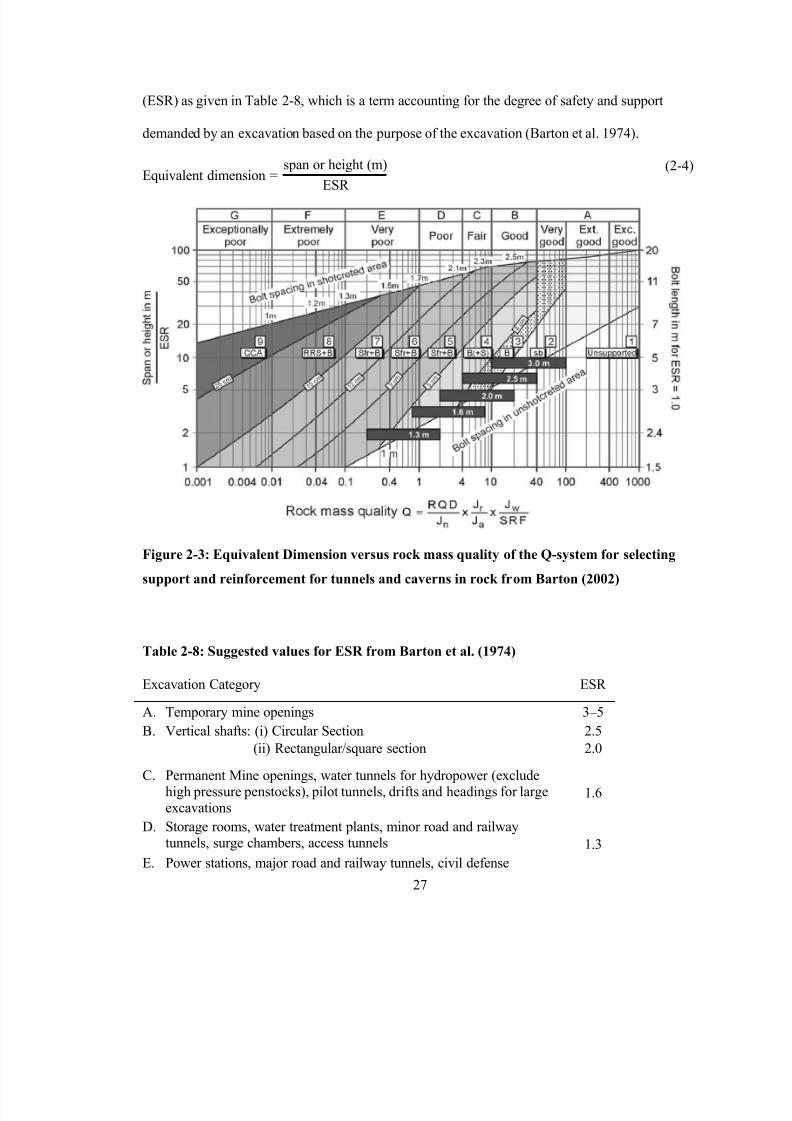
Figure 2-3: Equivalent Dimension versus rock mass quality of the Q-system for selecting support
and reinforcement for tunnels and caverns in rock from Barton (2002) ........................................ 27
Figure 2-4: Conceptual model of the components of the RMi classification system from
Palmstrøm (1995) .......................................................................................................................... 29
Figure 2-5: GSI classification chart from Marinos et al (2005) 34

8/11/2019 Numerical Validation and Refinement of Empirical Rock Mass Modulus
http://slidepdf.com/reader/full/numerical-validation-and-refinement-of-empirical-rock-mass-modulus 12/263
Figure 3-3: Classic post-failure characteristics for rock masses (a) Strain hardening (b) Elastic
perfectly plastic (c) Strain softening (d) Elastic-brittle .................................................................. 53
Figure 3-4: Four-noded "Goodman Joint Element" after Goodman et al. (1968) .......................... 56
Figure 3-5: Discontinuity curves with K n and K s values for (Left) Normal Stress vs. Closure
(Right) Shear Stress vs. Shear Displacement ................................................................................. 57
Figure 3-6: Block sketches of joint behaviour, under (Left) low normal stress leading to dilation
and (Right) high normal stress leading to shearing through asperities .......................................... 59
Figure 3-7: JRC values for 10cm scale roughness profiles from Hoek et al. (1995) ..................... 61
Figure 3-8: Material Softening Method. Dashed lines represent the stress path of the softened
material of the tunnel face, and the ground reaction curve represents the surrounding rock mass,
after Vlachopoulos (2009). ............................................................................................................ 63
Figure 3-9: Average Pressure Reduction Method. Dashed lines represent the stress path of the
internal pressure of the tunnel, and the ground reaction curve represents the rock mass, after
Vlachopoulos (2009). ..................................................................................................................... 64
Figure 3-10: LDP example relating tunnel wall displacements to the distance from the face from
Vlachopoulos & Diederichs (2009) ............................................................................................... 65
Figure 4-1: Stress-Strain curve of a rock mass undergoing loading and subsequent unloading - (1)
Initial tangent modulus (2) elastic tangent modulus (3) Recovery modulus (4) Erm from Hoek &
Diederichs (2006)........................................................................................................................... 71
Figure 4-2: Conceptual diagram for the post-processing of: (Left) The block model to obtain
stress and strain for the back calculation of Erm and (Right) The tunnel model to obtain an average
f h l di l h b d d b i l l 73

8/11/2019 Numerical Validation and Refinement of Empirical Rock Mass Modulus
http://slidepdf.com/reader/full/numerical-validation-and-refinement-of-empirical-rock-mass-modulus 13/263
Figure 4-7: Relationship between Jr of the Q-System and JRC for 20cm and 1m samples from
Hoek et al. (1995) .......................................................................................................................... 87
Figure 4-8: Sample block model geometry used in the block model analysis ............................... 89
Figure 4-9: Barton-Bandis strength criterion in τ – σn space, with joint planes for joints in model
and Mohr circles for appropriate stress states ................................................................................ 91
Figure 4-10: Scale sensitivity of Block Models (a) Smallest scale (b) Standard scale models used
for all block models (c) Medium-Large scale model (d) Largest scale model .............................. 93
Figure 4-11: Aspect ratio sensitivity in jointed block models (Left) 1:1 aspect ratio of jointed rockmass (Middle) 1.5:1 aspect ratio (Right) 2:1 aspect ratio .............................................................. 94
Figure 4-12: Joint orientation sensitivity in the "Very Blocky" model. Orientations of the joint
sets, with respect to the horizontal are as follows: (a) 30°, -30° and 90° (the base case used for all
"Very Blocky" structure models); (b) 15°, -45° and 75°; (c) 0°, -60° and 60°; (d) -15°, -75° and
45° .................................................................................................................................................. 96
Figure 4-13: A tunnel model at 1/4 symmetry ............................................................................... 97
Figure 4-14: Tunnel models for (Left) Very Blocky Jointed Rock mass (Right) Equivalent
Continuum Model .......................................................................................................................... 99
Figure 4-15: Jointed rock mass zone sizes extending from tunnel boundary. (Left) 3 tunnel
diameters (Centre) 5 tunnel diameters (Right) 8 tunnel diameters .............................................. 100
Figure 4-16: Model symmetry (Left) Full tunnel model (Right, Top) Half symmetry model
(Right, Bottom) Quarter symmetry model ................................................................................... 101
Figure 5-1: Summary of models covering the modelling GSI spectrum used for the block model
l i f M i l (2005) 105

8/11/2019 Numerical Validation and Refinement of Empirical Rock Mass Modulus
http://slidepdf.com/reader/full/numerical-validation-and-refinement-of-empirical-rock-mass-modulus 14/263
Figure 5-5: Results for load method sensitivity of distributed loads vs. nodal displacements along
the top boundary of the model. .................................................................................................... 108
Figure 5-6: Results of sensitivity analysis for given joint set orientations (in degrees), for "Very
Good" joint surface conditions (GSI 65). .................................................................................... 109
Figure 5-7: Results of sensitivity analysis for given joint set orientations (in degrees), for "Good"
joint surface conditions (GSI 55). ................................................................................................ 110
Figure 5-8: Results of sensitivity analysis for given joint set orientations (in degrees), for "Fair"
joint surface conditions (GSI 45). ................................................................................................ 110
Figure 5-9: Results of sensitivity analysis for given joint set orientations (in degrees), for "Poor"
joint surface conditions (GSI 35). ................................................................................................ 111
Figure 5-10: Results of sensitivity analysis for given joint set orientations (in degrees), for "Very
Poor" joint surface conditions (GSI 25). ...................................................................................... 111
Figure 5-11: Plot of modulus of deformation vs. GSI for the Generalized Hoek-Diederichs
equation and those back calculated from the block models (Top) Using a standard scale for Erm
(Bottom) Using a logarithmic scale for Erm. ................................................................................ 113
Figure 5-12: Conceptual model of the stress-strain curve for block models, and the differences in
Erm calculated for elastic joint models vs. plastic joint models. ................................................... 114
Figure 5-13: Results of model A1 (GSI 90) using elastic and plastic joint properties. ............... 115
Figure 5-14: Results of model A2 (GSI 80) using elastic and plastic joint properties. ............... 115
Figure 5-15: Results of model A3 (GSI 70) using elastic and plastic joint properties. ............... 116
Figure 5-16: Results of model B1 (GSI 75) using elastic and plastic joint properties. ................ 117
Fi 5 17 R l f d l B2 (GSI 65) i l i d l i j i i 117

8/11/2019 Numerical Validation and Refinement of Empirical Rock Mass Modulus
http://slidepdf.com/reader/full/numerical-validation-and-refinement-of-empirical-rock-mass-modulus 15/263
Figure 5-28: Results of model D3 (GSI 35) using elastic and plastic joint properties. ............... 123
Figure 5-29: Results of model D4 (GSI 25) using elastic and plastic joint properties. ............... 124
Figure 5-30: Results of model D5 (GSI 15) using elastic and plastic joint properties. ............... 124
Figure 6-1: Internal support pressure vs. average total tunnel wall displacements for models with
varying extent of the jointed rock mass, in terms of the number of tunnel diameters extending
from the tunnel wall boundary, for elastic joints (infinite strength). ........................................... 130
Figure 6-2: Internal support pressure vs. average total tunnel wall displacements for models with
varying extent of the jointed rock mass, in terms of the number of tunnel diameters extendingfrom the tunnel wall boundary, for joints with the Barton-Bandis shear strength criterion. ....... 130
Figure 6-3: Results for varying width of representative boundary in models, with joint shear
strength defined by the Barton-Bandis shear strength criterion. .................................................. 132
Figure 6-4: Results of sensitivity of model symmetry for models with elastic joint properties and
plastic joint properties. ................................................................................................................. 133
Figure 6-5: Summary of final tunnel wall displacements predicted in models with elastic joint and
elastic intact rock models compared to displacements predicted from the Carranza-Torres (2004)
analytical solution with elastic-only displacements. .................................................................... 135
Figure 6-6: Summary of final tunnel wall displacements predicted in models with plastic joint and
plastic intact rock properties compared to displacements predicted from the fully plastic
Carranza-Torres (2004) analytical solution ................................................................................. 136
Figure 6-7: Results for models of high intact rock strength in a 35 MPa hydrostatic stress field
(S1D1). ......................................................................................................................................... 137
Fi 6 8 R l f d l f hi h i k h i 20 MP h d i fi ld

8/11/2019 Numerical Validation and Refinement of Empirical Rock Mass Modulus
http://slidepdf.com/reader/full/numerical-validation-and-refinement-of-empirical-rock-mass-modulus 16/263
Figure 6-13: Results for models of low intact rock strength in a 35 MPa hydrostatic stress field
(S3D1). ......................................................................................................................................... 143
Figure 6-14: Results for models of low intact rock strength in a 20 MPa hydrostatic stress field
(S3D2). ......................................................................................................................................... 144
Figure 6-15: Results for models of low intact rock strength in a 5 MPa hydrostatic stress field
(S3D3). ......................................................................................................................................... 145
Figure 6-16: Comparison of yielding between a jointed rock mass model of "Very Blocky"
structure and "Very Poor" discontinuity surface conditions and the equivalent continuum model.(Left) Extent of yielded joint elements in a jointed rock mass model with plastic joints (Right)
Extent of yielded material elements in an equivalent plastic continuum model. ......................... 149
Figure 7-1: Stress/Strain response of a rock sample undergoing load for (i) Hard rock (ii) Soft
rock. Region 'A' is the non-linear portion due to initial closure of internal voids or micro cracks,
'B' is the linear elastic response to the loading of the sample, and 'C' is the inelastic portion of the
curve associated with the yield stress of the sample. ................................................................... 155
Figure 7-2: Proposed Generalized Hoek-Diederichs modification for Tunnels (Left) Erm vs GSI
plot using a correction factor Ce of Eq. (7-2) with D = 0 (Right) Erm vs GSI plot for Generalized
Hoek-Diederichs equation with D = 0. ........................................................................................ 157
Figure 7-3: Ratio of Erm predicted from correction equation (7-1) to the Generalized Hoek-
Diederichs estimation vs. GSI, with modifications of the exponent in Eq. (7-2) (Left) Using a
value of 0.5 (Right) Using a value of 0.6 ..................................................................................... 158
Figure 7-4: Proposed Generalized Hoek-Diederichs modification for Tunnels (Left) Erm vs GSI
l i i f f E (7 5) i h D 0 (Ri h ) E GSI l f G li d

8/11/2019 Numerical Validation and Refinement of Empirical Rock Mass Modulus
http://slidepdf.com/reader/full/numerical-validation-and-refinement-of-empirical-rock-mass-modulus 17/263
From Erm estimated using Eq. (7-4) (Right) From Erm estimated using original Generalized Hoek-
Diederichs equation reproduced from Figure 6-5. ....................................................................... 161

8/11/2019 Numerical Validation and Refinement of Empirical Rock Mass Modulus
http://slidepdf.com/reader/full/numerical-validation-and-refinement-of-empirical-rock-mass-modulus 18/263
List of Symbols and Acronyms
a Hoek-Brown Variable Coefficient
c Cohesion
Ce Hoek-Diederichs Correction Factor
D Disturbance Factor
D RMi Parameter Calculated from the Joint Condition Factor
DIANE Discontinuous, Inhomogeneous, Anisotropic and Non-Elastic
Erm Rock Mass modulus of deformation
Ei Young’s Modulus of Elasticity
FEM Finite Element Method
GHB Generalized Hoek-Brown Failure Criterion
Gi Intact Shear Modulus
Grm Rock Mass Shear Modulus
GSI Geological Strength Index system for classification of rock masses
jA Joint Surface Alteration
J J i Al i N b

8/11/2019 Numerical Validation and Refinement of Empirical Rock Mass Modulus
http://slidepdf.com/reader/full/numerical-validation-and-refinement-of-empirical-rock-mass-modulus 19/263
JRC Joint Roughness Coefficient
js Joint Small Scale Smoothness Factor
Js Joint Small-Scale Smoothness Factor
jw Large Scale Joint Plane Waviness Factor
Jw Joint Water Reduction Factor
Jw Joint Large-Scale Waviness Factor
K n Joint Normal Stiffness
K s Joint Shear Stiffness
LDP Longitudinal Displacement Profile
m b Hoek-Brown Reduced Value of the Material Constant mi
mi Hoek-Brown Material Constant for Intact Rock
MR Modulus Ratio
PDE Partial Differential Equation
pi Internal Support Pressure
p0 Hydrostatic Pressure
PJT Plate Jacking Test

8/11/2019 Numerical Validation and Refinement of Empirical Rock Mass Modulus
http://slidepdf.com/reader/full/numerical-validation-and-refinement-of-empirical-rock-mass-modulus 20/263
s Hoek-Brown Material Constant
SRF Stress Reduction Factor
u Joint Undulation
UCS Unconfined compressive strength
Ur Radial Inward Convergence
V b Average Block Volume
ν Poisson’s Ratio
RQD Rock Quality Designation
ε Strain
ϕ Joint Friction Angle
ϕr Residual Friction Angle
σ1 Major principal stresss
σ3 Minor principal stress
σci Unconfined compressive strength of intact rock
σn Normal Stress
σrr Radial Stress

8/11/2019 Numerical Validation and Refinement of Empirical Rock Mass Modulus
http://slidepdf.com/reader/full/numerical-validation-and-refinement-of-empirical-rock-mass-modulus 21/263
Chapter 1
Introduction
1.1 Background
Numerical modelling programs have proven to be very useful tools for engineers to model the
complex behaviour of a rock mass undergoing some form of field stress change induced by the
excavation of an underground opening or tunnel. As more reliance is placed on the output of
numerical simulation for the design of the excavation sequencing, reinforcement and support
requirements, it is critical that careful consideration be given to the input parameters. The model
input parameters are obtained from results of lab testing, geotechnical site investigations or
derived by empirical methods. Current day computing resources are too limited to be able to
process all relevant information collected in a detailed site geotechnical investigation. In order to
properly analyze the problem domain, a representative behaviour of the rock mass is assumed by
assigning representative values to the input parameters. At their fundamental level, most Finite
Element Method (FEM) numerical analysis programs require representative input parameters that
describe the strength and deformability of the rock mass (Figure 1-1).

8/11/2019 Numerical Validation and Refinement of Empirical Rock Mass Modulus
http://slidepdf.com/reader/full/numerical-validation-and-refinement-of-empirical-rock-mass-modulus 22/263
can then be used in the design for the excavation methods, as well as the support and
reinforcement requirements for the tunnel.

8/11/2019 Numerical Validation and Refinement of Empirical Rock Mass Modulus
http://slidepdf.com/reader/full/numerical-validation-and-refinement-of-empirical-rock-mass-modulus 23/263
rock conditions likely to occur between respective sites. Rock mass classification systems
combine such parameters to quantitatively describe a given rock mass (Figure 1-2). Four
different rockmass classification systems have been defined that are applicable for tunnelling
applications, including the Rock Mass Quality (Q) system, the Rock Mass Rating (RMR), the
Geological Strength Index (GSI) and the Rock Mass Index (RMi) system. Each have their merits
based on the specific case studies that were used for their initial conception. The quantitative
information that these systems provide can be used in order to predict the anticipated response of
a rock mass with respect to the tunnelling excavation.

8/11/2019 Numerical Validation and Refinement of Empirical Rock Mass Modulus
http://slidepdf.com/reader/full/numerical-validation-and-refinement-of-empirical-rock-mass-modulus 24/263
Erm is a representative parameter commonly used in FEM programs, which describes the ratio of
stress to corresponding strain during loading of a rock mass, and includes both elastic and
inelastic behaviour. A site-specific determination of Erm is usually conducted by compressional
testing methods in exploratory adits (Figure 1-3), such as the Plate Jacking Test (PJT), the Plate
Loading Test (PLT) and the Radial Jacking Test (Bieniawski 1978, Palmstrøm & Singh 2001).
These tests are difficult to conduct, require a significant amount of time and are very expensive.
Consequently, they are seldom conducted in most civil and mining engineering projects related to
underground excavations.

8/11/2019 Numerical Validation and Refinement of Empirical Rock Mass Modulus
http://slidepdf.com/reader/full/numerical-validation-and-refinement-of-empirical-rock-mass-modulus 25/263
As an alternative to direct testing methods, Erm can be estimated from empirical
relationships from the quantitative output of engineering rock mass classification systems.
Numerous such relationships have been proposed for rock mass classification systems such as Q
(Barton 2002), RMR (Bieniawski 1978, Serafim & Pereira 1983), GSI (Hoek et al. 2002, Sonmez
et al. 2004, Hoek & Diederichs 2006) and RMi (Palmstrøm & Singh 2001). These relationships
were derived on the basis of curve fitting to case histories, and it is important to note that they
assume that the rock mass is isotropic. This is not usually always the case, as situations exist
such as laminated rock for which the rockmass behaves in an anisotropic fashion. Nonetheless,
these types of relationships can still effectively be used.
1.2
Research Objectives
1.2.1
Numerical Assessments of the Hoek-Diederichs Empirical Rock Mass Modulus of
Deformation Formula
The Generalized Hoek-Diederichs Empirical formula (Hoek & Diederichs 2006) for rock mass
modulus of deformation estimation using the GSI rock mass classification system was derived
from a large database of in situ measurements from China and Taiwan (Figure 1-4).
The Generalized Hoek-Diederichs empirical relationship is based on a sigmoid function

8/11/2019 Numerical Validation and Refinement of Empirical Rock Mass Modulus
http://slidepdf.com/reader/full/numerical-validation-and-refinement-of-empirical-rock-mass-modulus 26/263
(2008) suggests relationships between Erm and GSI are unlikely to be reliable for values of GSI
less than 30.
Figure 1-4: (Left) General GSI rock mass classification chart after Marinos et al. (2005);
(Right) Data plot of Simplified Hoek-Diederichs equation from Hoek & Diederichs (2006)

8/11/2019 Numerical Validation and Refinement of Empirical Rock Mass Modulus
http://slidepdf.com/reader/full/numerical-validation-and-refinement-of-empirical-rock-mass-modulus 27/263
range of rock mass quality is tested over several combinations of stress regimes and different
strengths of the intact rock.
Figure 1-5: Ranges of GSI and the number of in situ tests contained within the Taiwanese
and Chinese dataset used in the derivation of the Generalized Hoek-Diederichs empirical
relationship
1.2.2
FEM Numerical Model Representation of GSI Rock Mass Classification System
The 2-dimensional FEM program Phase² 7.0 (Rocscience Inc. 2010) is used for this research in

8/11/2019 Numerical Validation and Refinement of Empirical Rock Mass Modulus
http://slidepdf.com/reader/full/numerical-validation-and-refinement-of-empirical-rock-mass-modulus 28/263
Surface conditions are controlled by varying the joint normal and joint shear stiffness parameters
as well as their strength universally.
The FEM numerical model development undertaken for this research was historically
very difficult, if not impossible, due to the lack of ample computer processing capabilities and the
reduced functionality of the FEM programs themselves. Recent developments in FEM numerical
modelling programs have enhanced the joint network generation and simplified the mesh
generation process, which has been important to the timely generation and computation of the
numerical models for this research. This point is significant when conducting parametric analysis
to calibrate the joints within the models, as the joint networks dominate the behaviour of the rock
mass. Therefore it is essential to correctly assign their properties.
1.2.3
Joint Input Parameter Calibration from Block Models
In order to calibrate the methodology for the assignment of joint properties, simple block models
are created in the form of an unconfined compressive strength (UCS) test in Phase2. It is assumed
that the Hoek-Diederichs empirical relationship is correct for the 40-80 GSI range as discussed in
Section 1.2.1, and the calibration is achieved by ensuring a back-calculated value for Erm from the
stress and strain in the block model is the same for this GSI range as the empirically determined

8/11/2019 Numerical Validation and Refinement of Empirical Rock Mass Modulus
http://slidepdf.com/reader/full/numerical-validation-and-refinement-of-empirical-rock-mass-modulus 29/263
to generate rock masses of varying quality based on a GSI characterization between 40-80 that
show a deformational response very similar to an empirically-estimated, GSI – based Erm value by
calibrating the normal and shear stiffness parameters. These parameters, when applied to higher
quality, non-persistent block models show a stiffer response than an empirically estimated, GSI-
based representative Erm value on the basis of the Hoek-Diederichs empirical relationship. In
poorer quality rock masses, the block models show a considerably softer response.
The numerical analysis and closure predictions of a tunnel can differ when the rock mass
includes an explicit representation of the major discontinuities versus a representative, non-
jointed continuum rock mass with a reduced modulus. This research shows that the degree of
variation depends on both the stress regime resulting from the depth at which the tunnel is to be
excavated, as well as the strength of the intact rock between the major discontinuities. Models in
this analysis show that in stronger intact rock, larger tunnel displacements occur in poorer quality
rock masses when the discontinuities behave plastically than are predicted in the equivalent,
continuum based models. In contrast, the results show that in weaker intact rock, continuum
models overestimate the amount of tunnel closure in comparison to their jointed rock mass
equivalents. When both continuum and jointed models behave entirely elastically, in poor quality

8/11/2019 Numerical Validation and Refinement of Empirical Rock Mass Modulus
http://slidepdf.com/reader/full/numerical-validation-and-refinement-of-empirical-rock-mass-modulus 30/263
presented in relevant sections and subsections. References used within each chapter are given in
full at the end of each chapter.
Chapter 2 reviews the concepts of rock mass classification systems and their significance
to tunnelling applications. Major and commonly used rock mass classification systems, which
include the Rock Quality Designation (RQD) (Deere 1968), Rock Mass Rating system (RMR)
(Bieniawski 1973, 1976, 1989), the Rock Mass Quality system (Q) (Barton et al. 1974), the Rock
Mass Index system (RMi) (Palmstrøm 1995) and the Geological Strength Index (GSI) (Hoek
1994, Hoek et al. 1995, Hoek & Marinos 2000, Marinos et al. 2005, Hoek et al. 2005), are
described according to their latest and most common versions. This is followed by a discussion
of how rock mass classification systems can be used for input parameter estimation in numerical
modelling programs. The chapter concludes with a discussion of analytical tools used for tunnel
closure prediction, their limitations, and the importance of numerical analysis for tunnel closure
predictions.
Chapter 3 provides a literature review of the theory of FEM numerical analysis. A brief
description of elasticity and plasticity models are discussed, as well as the numerical
representation of discontinuities in FEM models including their stiffness and strength properties.

8/11/2019 Numerical Validation and Refinement of Empirical Rock Mass Modulus
http://slidepdf.com/reader/full/numerical-validation-and-refinement-of-empirical-rock-mass-modulus 31/263
Chapter 5 presents the results of the sensitivity analysis and the results of the block
models that were used for the calibration of input parameters, as well as for the sensitivity
analysis. A discussion and interpretation on the results is included at the end.
Chapter 6 is a high-level overview of the results of all tunnel models, within the context
of the determined final tunnel wall closure. The meaning of the results is discussed as a
conclusion to this chapter.
A discussion and explanation of all modelling results is made in Chapter 7. Here a
proposed modification to the Generalized Hoek-Diederichs empirical relationship is made for
tunnelling applications. A summary of the major findings and suggested future work will also be
discussed.
1.5 References
Barton, N. (2002). Some New Q-Value Correlations to Assist in Site Characterisation and Tunnel
Design. Int J Rock Mech Mining Sci, 39(2), 185-216.
Barton, N., Lien, R., & Lunde, J. (1974). Engineering Classification of Rock Masses for the
Design of Tunnel Support. Rock Mech, 6, 183-236.
Bieniawski, Z. (1973). Engineering Classification of Jointed Rock Masses. The Civil Engineer in
South Africa, pp. 335-343.

8/11/2019 Numerical Validation and Refinement of Empirical Rock Mass Modulus
http://slidepdf.com/reader/full/numerical-validation-and-refinement-of-empirical-rock-mass-modulus 32/263
Hoek, E., & Diederichs, M. (2006). Empirical Estimation of Rock Mass Modulus. Int J Rock
Mech Mining Sci, 43(2), 203-215.
Hoek, E., & Marinos, P. (2000). GSI: A Geologically Friendly Tool for Rock Mass Strength
Estimation. Proc. GeoEng2000 Conference (pp. 1422-1446). Melbourne: Technomic publishers.
Hoek, E., Carranza-Torres, C., & Corkum, B. (2002). Hoek-Brown Failure Criterion - 2002
Edition. In R. Hammah, W. Bawden, J. Curran, & M. Telesnicki (Ed.), proceedings of the 5th
North American Rock Mechanics Symposium and the 17th Tunnelling Association of Canada
Conference, NARMS-TAC 2002. Toronto: University of Toronto Press.
Hoek, E., Kaiser, P., & Bawden, W. (1995). Support of Underground Excavations in Hard Rock.
Rotterdam: Balkema.
Hoek, E., Marinos, P., & Marinos, V. (2005). Characterisation and Engineering Properties of
Tectonically Undisturbed but Lithologically Varied Sedimentary Rock Masses. Int J Rock Mech
Mining Sci, 42, 277-285.
Hutchinson, J., & Diederichs, M. (1996). Cablebolting in Underground Mines. Richmond, British
Columbia, Canada: BiTech Publishers Ltd.
Marinos, P. (2010). Personal Communications.
Marinos, V., Marinos, P., & Hoek, E. (2005). The Geological Strength Index: Applications and
Limitations. Bull Eng Geol Environ, 64, 55-65.
Palmstrøm, A. (1995). RMi - A Rock Mass Characterization System for Rock Engineering
Purposes. University of Oslo, Norway.
Palmstrøm, A., & Singh, R. (2001). The Deformation Modulus of Rock Masses – Comparisons
Between In Situ Tests and Indirect Estimates Tunnelling Underground Space Technol 16(2)

8/11/2019 Numerical Validation and Refinement of Empirical Rock Mass Modulus
http://slidepdf.com/reader/full/numerical-validation-and-refinement-of-empirical-rock-mass-modulus 33/263

8/11/2019 Numerical Validation and Refinement of Empirical Rock Mass Modulus
http://slidepdf.com/reader/full/numerical-validation-and-refinement-of-empirical-rock-mass-modulus 34/263
Rock mass classification systems provide a framework for standardizing the data
collection mechanisms related to the geotechnical site investigation. This ensures that all relevant
data has been collected as efficiently and concisely as possible. The quantitative output provided
is then used for further empirical design such as the support requirements, excavation methods
and sequencing, or as input for use in numerical modelling programs. The latter is the subject of
this research.
2.1.2
Rock Quality Designation (RQD)
One of the earlier rock mass classification systems is the Rock Quality Designation (RQD) as
proposed by Deere et al. (1967) and Deere & Deere (1988), developed for estimation of rock
mass quality in situ from drill core logs. The RQD calculation is defined as a percentage of the
lengths of 10cm or greater intact core pieces in the total length of core (Figure 2-1). Artifacts of
the drilling process, such as core discing or drilling breaks should be ignored. The total length of
core also includes any sections of lost core (Figure 2-2).
RQD estimations are entirely dependent upon the orientation of the drill core. This can
especially be a problem in rock masses that are highly anisotropic with one dominant
discontinuity set such as bedding planes, for which core oriented parallel to the bedding planes

8/11/2019 Numerical Validation and Refinement of Empirical Rock Mass Modulus
http://slidepdf.com/reader/full/numerical-validation-and-refinement-of-empirical-rock-mass-modulus 35/263
Figure 2-1: The measurement and calculation of RQD from Hoek et al. (1995)

8/11/2019 Numerical Validation and Refinement of Empirical Rock Mass Modulus
http://slidepdf.com/reader/full/numerical-validation-and-refinement-of-empirical-rock-mass-modulus 36/263
Approaches to the estimation of RQD in the event where core is not available have also
been proposed. On the basis of the volumetric joint count (Jv) or the total number of joints per
m3, a theoretical correlation has been proposed by Palmstrøm (1982) for 3 or more joint sets as
follows:
RQ 33v (2-1)
where v is calculated on the basis of the true spacing for each of the major joint sets present. For
3 well defined joint sets with spacings of S1, S2 and S3 intersecting at right angles, Eq. (2-2) for v
is given as follows (Palmstrøm 1995):
v
S
S
S3
(2-2)
RQD is a simple means for providing a quantitative index of the structure of the rock
mass; however it does not provide a comprehensive description as other geological parameters
such as hydrological conditions, joint orientation and joint surface conditions are not included.
RQD is included as a key input parameter in other rock mass classification systems.
2.1.3
Rock Mass Rating System (RMR)
2.1.3.1
Description

8/11/2019 Numerical Validation and Refinement of Empirical Rock Mass Modulus
http://slidepdf.com/reader/full/numerical-validation-and-refinement-of-empirical-rock-mass-modulus 37/263
- Condition of discontinuities
- Groundwater conditions
- Orientation of discontinuities
The rock mass is first divided into a number of discrete regions, so that each region is
geologically and geomechanically similar. The information collected in the field on these six
parameters is assessed according to a relative weighting system on the basis of their respective
values. The first five parameters are assigned a non-negative weighting from Tables 2-1 and 2-2.
The sixth parameter is an adjustment accounting for the attitude of discontinuities with respect to
the engineering excavation, which is assigned a non-positive value from Tables 2-4 and 2-3. The
assessment of the last four parameters related to discontinuities is completed on the major
discontinuity set that will have the most influence on the stability of the application. If no major
set is identified, then the ratings for each set are averaged in the determination of the
classification parameter.

8/11/2019 Numerical Validation and Refinement of Empirical Rock Mass Modulus
http://slidepdf.com/reader/full/numerical-validation-and-refinement-of-empirical-rock-mass-modulus 38/263
Table 2-1: RMR 76 and RMR 89 Classification Parameters and Ratings after Bieniawski
(1976, 1989) and Hoek et al. (1995)
1
Strength of intact rock
material
Point-load strength index
>8 MPa
(RMR 76)
>10MPa
(RMR 89)
4-8 MPa
(RMR 76)
4-10 MPa
(RMR 89)
2-4 MPa 1-2 MPaUCS test preferred in
this range
Uniaxial Compressive
strength (RMR 76)>200 MPa
100 – 200
MPa50 – 100 MPa 25 – 50 MPa
10-25
MPa
3-10
MPa
1-3
MPa
Uniaxial compressive
strength (RMR 89)>250 MPa
100 – 250
MPa50 – 100 MPa 25 – 50 MPa
5-25
MPa
1-5
MPa
<1
MPa
Rating (RMR 76 and RMR 89) 15 12 7 4 2 1 0
2Drill core quality RQD (%) 90 – 100 75 – 90 50 – 75 25 – 50 <25
Rating (RMR 76 and RMR 89) 20 17 13 8 3
3Spacing of
Discontinuities
RMR 76 >3 m
1 – 3 m 0.3 – 1 m 50 – 300 mm <50 mm
Rating 30 25 20 10 5
RMR 89 >2 m 0.6 – 2 m 200 – 600 mm 60 – 200 mm <60 mm
Rating 20 15 10 8 5
4
Condition of
Discontinuities
(for RMR 89 see
additional Table 2-2)
RMR 76
Very roughsurfaces
Not continuous No Separation
Hard joint wallrock
Slightly roughsurfaces
Separation< 1 mm
Hard joint wallrock
Slightly roughsurfaces
Separation
< 1 mm
Soft joint wall rock
Slickensided surfacesor
Gouge < 5mm thickor Joints open
1-5mm
Continuous joints
Soft gouge > 5mm thick or
Joints open > 5mm
Continuous joints
Rating 25 20 12 6 0
RMR 89
Very roughsurfaces
Not continuous
No Separation
Unweateredwall rock
Slightly roughsurfaces
Separation
< 1 mm
Slightlyweathered wall
Slightly rough
surfaces
Separation < 1 mm
Highly weatheredwall
Slickensided surfacesor
Gouge < 5mm thickor Separation
1-5mm
continuous
Soft gouge > 5mm thick or
Separation > 5mm
Continuous
Rating 30 25 20 10 0
Inflow per 10m tunnel
length None <25 litres/min
25 – 125
litres/min>125 litres/min
Ratio:
0 0.0 – 0.2 0.2 – 0.5 >0.5
8/11/2019 Numerical Validation and Refinement of Empirical Rock Mass Modulus
http://slidepdf.com/reader/full/numerical-validation-and-refinement-of-empirical-rock-mass-modulus 39/263
Table 2-2: RMR 89 Guidelines for Classification of Discontinuity Conditions from Bieniawski
(1989)
Parameter Ratings
Discontinuity length
(persistence/continuity)
<1 m
6
1 – 3 m
4
3 – 10 m
2
10 – 20 m
1
>20 m
0
Separation (aperture) None
6
<0.1 mm
5
0.1 – 1.0 mm
4
1 – 5 mm
1
>5 mm
0
RoughnessVery rough
6
Rough
5
Slightly rough
3
Smooth
1
Slickensided
0
Infilling (gouge) None6
Hard filling Soft filling
<5 mm
4
>5 mm
2
<5 mm
2
>5 mm
0
Weathering Unweathered
6
Slightly weathered
5
Moderately
weathered
3
Highly
weathered
1
Decomposed
0
*Some conditions are mutually exclusive. For example, if infilling is present, it is irrelevant what the roughness may be, since its effect will be
overshadowed by the influence of the gouge. In such cases, use Table 2-1 directly.
Table 2-3: RMR 76 and RMR 89 Discontinuity Attitude and Effect in Tunnelling, from
Bieniawski (1989)
Strike Perpendicular to Tunnel Axis
Drive with Dip Drive against Dip
Dip 45 – 90 Dip 20 – 45 Dip 45 – 90 Dip 20 – 45
Very favorable Favorable Fair Unfavorable
Strike Parallel to Tunnel Axis Irrespective of Strike
Dip 20 – 45 Dip 45 – 90 Dip 0-20

8/11/2019 Numerical Validation and Refinement of Empirical Rock Mass Modulus
http://slidepdf.com/reader/full/numerical-validation-and-refinement-of-empirical-rock-mass-modulus 40/263
2.1.3.2 Applications and Limitations
The original 1973 form of the RMR system was limited to being applicable to tunnelling only,
because only 49 case histories were investigated by Bieniawski (1976, 1989). As more case
histories became available, the system was extended to include dam foundations, mining and
slopes. For the purposes of excavation and initial support recommendations however, the only
empirical design published is for tunnelling specific applications. Table 2-5 is used to classify the
rock mass and provides some strength and standup time estimations based on the classification.
The RMR tables illustrate the key differences between the RMR 76 and RMR 89 systems. When
using RMR as a basis for empirical rock mass parameters, such as deformation modulus, it is very
important to be aware of these modifications and their meaning to the application of interest.
Table 2-5: RMR 76 and RMR 89 Rock Mass Classes and their Meaning after Bieniawski
(1976, 1989)
ROCK MASS CLASSES DETERMINED FROM TOTAL RATINGS
Rating 10081 80 61 60 41 40 21 <20
Class no. I II III IV V
Description Very good rock Good rock Fair rock Poor rock Very poor rock
MEANING OF ROCK MASS CLASSES
Class no. I II III IV V
Average stand-up time 10 yr. for 5 m span 6 mo. for 4 m span 1 wk. for 3 m span 5h for 1.5 m span 10 min for 0.5 m span

8/11/2019 Numerical Validation and Refinement of Empirical Rock Mass Modulus
http://slidepdf.com/reader/full/numerical-validation-and-refinement-of-empirical-rock-mass-modulus 41/263
greater than 1000m, or where the ratio of the unconfined compressive strength (σci to the major
principal stress σ
is less than 4, the consideration of stress becomes important for mining
tunnels and chambers. These limitations have led to modifications to RMR specific to hard rock
mining, such as the Modified Rock Mass Rating (MRMR) system for asbestos mining in southern
Africa and the MBR (modified Basic RMR) system for U.S. copper mining (Bieniawski 1989,
Hoek et al. 1995).
2.1.4
Rock Mass Quality (Q)
2.1.4.1 Description
The Q-system of rock mass classification and support design was developed over the course of
1973 to 1974 from over 212 case records of tunnels from 1960-1973 in Scandinavia (Barton
1976, 2002). No changes have been made to its original 1974 form. It is comprised of six
parameters for use in the evaluation of a rock mass, combined into Eq. (2-3):
Q RQ
n
r
a
w
SR
(2-3)
where
RQD is the Rock Quality Designation

8/11/2019 Numerical Validation and Refinement of Empirical Rock Mass Modulus
http://slidepdf.com/reader/full/numerical-validation-and-refinement-of-empirical-rock-mass-modulus 42/263
is the relative effect of water, faulting, squeezing, swelling and the strength to stress ratio. The
information collected in the field on these six parameters is assessed according to a relative
weighting system on the basis of their respective values, which is summarized in Table 2-6 ϕr
represents the residual friction angle in this table. Some additional notes on the usage of this
table are provided in Table 2-7. The parameters are used to describe the key discontinuity on
which failure is most likely to initiate. This is an implicit consideration for orientation relative to
the excavation (Barton 1976).
Table 2-6: Description and parameter ratings of the Q-System from Barton et al. (1974)
1. ROCK QUALITY DESIGNATION (RQD)
Very poor 0 – 25 Note:
(i)
Where RQD is reported or
measured as < 10 (including
0) a nominal value of 10 is
used to evaluate Q in Eq. (1)
(ii)
RQD intervals of 5, i. e. 100,
95, 90, etc. are sufficiently
accurate
Poor 25 – 50
Fair 50 – 75
Good 75 – 90
Excellent 90 – 100
2. JOINT SET NUMBER (Jn)

8/11/2019 Numerical Validation and Refinement of Empirical Rock Mass Modulus
http://slidepdf.com/reader/full/numerical-validation-and-refinement-of-empirical-rock-mass-modulus 43/263

8/11/2019 Numerical Validation and Refinement of Empirical Rock Mass Modulus
http://slidepdf.com/reader/full/numerical-validation-and-refinement-of-empirical-rock-mass-modulus 44/263
Table 2-6: Description and parameter ratings of the Q-System from Barton et al. (1974)
H. Medium or low over-consolidation, softening,clay mineral fillings. (Continuous, < 5 mm in
thickness)
8.0 (12° – 16°)
J. Swelling clay fillings, i. e. montmorillonite
(Continuous, < 5 mm in thickness). Value of Ja
depends on percent of swelling clay-size particles,
and access to water etc.
8.0 – 12.0 (6° – 12°)
(c) No rock wall contact when sheared
K,L,M. Zones or bands of disintegrated orcrushed rock and clay (see G, or H, J for
description of clay condition)
6.0, 8.0 or8.0 – 12.0
(6° – 24°)
N. Zones or bands of silty- or sandy clay, small
clay fraction (non-softening)
5.0
O,P,R. Thick, continuous zones or bands of clay
(see G, H, J for description of clay condition)
10.0, 13.0 or
13.0 – 20.0
(6° – 24°)
5. JOINT WATER REDUCTION FACTOR (Jw) Approx. water
pressure
(kg/cm2)
A. Dry excavations or minor inflow, i. e.
< 5 l/min. locally
1.0 < 1 Note:
(i)
Factors C to F are crude
estimates. Increase Jw if
drainage measures are
installed
(ii)
Special problems caused byice formation are not
considered
B. Medium inflow or pressure occasional outwash
of joint fillings
0.66 1.0 – 2.5
C. Large inflow or high pressure in competentrock with unfilled joints
0.5 2.5 – 10.0
D. Large inflow or high pressure, considerable
outwash of joint fillings
0.33 2.5 – 10.0

8/11/2019 Numerical Validation and Refinement of Empirical Rock Mass Modulus
http://slidepdf.com/reader/full/numerical-validation-and-refinement-of-empirical-rock-mass-modulus 45/263
Table 2-6: Description and parameter ratings of the Q-System from Barton et al. (1974)
very loose surrounding rock (any depth)B. Single weakness zones containing clay, or
chemically disintegrated rock (depth of
excavation ≤ m
5.0
C. Single weakness zones containing clay, or
chemically disintegrated rock (depth of
excavation >50 m)
2.5
D. Multiple shear zones in competent rock
(clay free), loose surrounding rock (any depth)
7.5
E. Single shear zones in competent rock (clay
free depth of excavation ≤ m
5.0
F. Single shear zones in competent rock (clay
free) (depth of excavation >50 m)
2.5
G. Loose open joints, heavily jointed or "sugar
cube" etc. (any depth)
5.0
(b) Competent rock, rock stress problems
σcσ1 σtσ1 (ii)
For strongly anisotropic
stress field (if measured):
when ≤σ1σ3≤, reduce σc
and σt to 8 σc and 8 σt;
when σ1σ3>, reduce σc
and σt to σc and σt
where: σc = unconfined
compression strength, σt =
tensile strength (point load),σ1 and σ3 = major and minor
principal stresses
(iii)
Few case records available
h d h f
H. Low stress, near-
surface
> 200 > 13 2.5
J. Medium stress 200 – 10 13 – 0.66 1.0
K. High stress, very tight
structure (Usually
favourable to stability,
may be unfavourable towall stability)
10 – 5 0.66 – 0.33 0.5 – 2.0
L. Mild rock burst
(massive rock)
5 – 2.5 0.33 – 0.16 5 – 10

8/11/2019 Numerical Validation and Refinement of Empirical Rock Mass Modulus
http://slidepdf.com/reader/full/numerical-validation-and-refinement-of-empirical-rock-mass-modulus 46/263
Table 2-7: Additional Notes on the Use of Table 2-7 from Barton et al. (1974)
When making estimates of the rock mass quality (Q) the following guidelines should be followed, in
addition to the notes listed in Table 2-6:
1. When core is unavailable, RQD can be estimated from the number of joints per unit volume, in which
the number of joints per metre for each joint set are added. A simple relation can be used to convert this
number to RQD for the case of clay-free rock masses – see Eq. (2-1), where (RQD = 100 for Jv < 4.5)
2. The parameter Jn, representing the number of joint sets will often be affected by foliation, schistocity,
slatey cleavage or bedding etc. If strongly developed these parallel "joints" should obviously be counted as
a complete joint set. However, if there are few "joints" visible, or only occasional breaks in core due to
these features, then it will be more appropriate to count them as "random joints" when evaluating J n in
Table 2-6.
3. The parameters Jr and Ja (representing shear strength) should be relevant to the weakest significant joint
set or clay filled discontinuity in a given zone. However, if the joint set or discontinuity with the minimum
value of (Jr /Ja) is favourably oriented for stability, then a second, less favourably oriented joint set or
discontinuity may sometimes be of more significance, and its higher value of (J r /Ja) should be used when
evaluating Q from Eq. (2-3).
4. When a rock mass contains clay, the factor SRF appropriate to loosening loads should be evaluatedusing Table 2-6, 6 (a). In such cases the strength of the intact rock is of little interest. However, when
jointing is minimal and clay is completely absent, the strength of the intact rock may become the weakest
link, and the stability will then depend on the ratio of rock-stress/rock-strength Table 2-6, 6 (b). A strongly
anisotropic stress field is unfavourable to stability and is accounted for as in note (ii), Table 2-6, 6 (b).
n general the compressive and tensile strengths σc and σt) of the intact rock should be evaluated in the
direction that is unfavourable for stability. This is especially important in the case of strongly anisotropic
rocks. In addition, the test samples should be saturated if this condition is appropriate to present or future
in situ conditions. A very conservative estimate of strength should be made for those rocks that deterioratewhen exposed to moist or saturated conditions.
2 1 4 2 Application and Limitations
8/11/2019 Numerical Validation and Refinement of Empirical Rock Mass Modulus
http://slidepdf.com/reader/full/numerical-validation-and-refinement-of-empirical-rock-mass-modulus 47/263

8/11/2019 Numerical Validation and Refinement of Empirical Rock Mass Modulus
http://slidepdf.com/reader/full/numerical-validation-and-refinement-of-empirical-rock-mass-modulus 48/263
chambers, portals, intersections 1.0
F. Underground nuclear power stations, railway stations, sports and public facilities, factories 0.8
2.1.5
Rock Mass Index (RMi)
2.1.5.1
Description
RMi was compiled by Dr. Arild Palmstrøm for his PhD thesis in 1995. It is considered as a
general strength characterization of the structural material that a rock mass represents, so that it
may be used for the purposes of construction (Palmstrøm 1995, 1996a). The general strength
characterization is composed of four input parameters, and the consideration of faults, shear
zones and dykes should be considered separately (Palmstrøm 1996a):
- The size of the blocks delineated by joints (block volume)
- The strength of the block material (uniaxial compressive strength)
- The shear strength of the block faces (friction angle)
- The size and termination of the joints (length and continuity)
Conceptually, the four parameters representing the average condition of the rock mass are
combined directly and indirectly as shown in Figure 2-4 to estimate an RMi value.

8/11/2019 Numerical Validation and Refinement of Empirical Rock Mass Modulus
http://slidepdf.com/reader/full/numerical-validation-and-refinement-of-empirical-rock-mass-modulus 49/263
Figure 2-4: Conceptual model of the components of the RMi classification system from
Palmstrøm (1995)
The parameter JP is further broken down and defined by Eq. (2-6):
P √ jVb
(2-6)
where Vb is the average block volume, given in units of m3, is calculated from Eq. (2-8), and
j is the joint condition factor expressed in Eq. (2-7):
j j
jR
j
(2-7)
3j
(2-8)
where j jR and j are factors for joint length and continuity joint wall roughness and joint

8/11/2019 Numerical Validation and Refinement of Empirical Rock Mass Modulus
http://slidepdf.com/reader/full/numerical-validation-and-refinement-of-empirical-rock-mass-modulus 50/263
1 – 10 m medium Joint 1 2
10 – 30m long/large Joint 0.75 1.5
> 30 m very long/large filled joint or seam
*
0.5 1*Often a singularity, and should in these cases be treated separately.
Table 2-10: The joint alteration factor (jA) from Palmstrøm (1995)
A. Contact Between the Two Rock Wall Surfaces
Term Description jA
Clean joints
-Healed or "welded" joints
Softening, impermeable filling (quartz, epidote etc.) 0.75
-Fresh rock walls No coating or filling on joint surface, except staining 1
-Alteration of jointwall:
1 grade more altered The joint surface exhibits one class higher alteration thanthe rock
2
2 grades morealtered
The joint surface shows two classes higher alteration thanthe rock
4
Coating or thin filling
-Sand, silt, calcite etc. Coating of friction materials without clay 3
-Clay, chlorite, talc
etc.
Coating of softening and cohesive minerals 4
B. Filled Joints with Partial or No Contact Between the Rock Wall Surfaces

8/11/2019 Numerical Validation and Refinement of Empirical Rock Mass Modulus
http://slidepdf.com/reader/full/numerical-validation-and-refinement-of-empirical-rock-mass-modulus 51/263
Palmstrøm (1995) also further breaks down the jR parameter into the small scale
smoothness factor ( js) and the large scale planarity of the joint plane waviness factor ( jw) with
respect to the surfaces of the joints as the expression in Eq. (2-9). Tables 2-11 and 2-12 provide
the definitions for js and jw respectively.
jR jsjw (2-9)
Table 2-11: Characterization of the smoothness factor (js) from Palmstrøm (1995)
Term Description js
Very rough Near vertical steps and ridges occur with interlocking effect
on the joint surface. 3
Rough Some ridge and side-angle steps are evident; asperities are
clearly visible; discontinuity surface feels very abrasive (likesandpaper grade approx.< 30).
2
Slightly rough Asperities on the discontinuity surfaces are distinguishable
and can be felt (like sandpaper grade approx. 30 - 300). 1.5
Smooth Surface appears smooth and feels so to the touch (smootherthan sandpaper grade approx. 300).
1
Polished Visual evidence of polishing exists, or very smooth surface asis often seen in coatings of chlorite and specially talc.
0.75
Slickensided Polished and often striated surface that results from frictionalong a fault surface or other movement surface.
0.6 – 1.5
Table 2-12: Characterization of the waviness factor (jw) from Palmstrøm (1995)

8/11/2019 Numerical Validation and Refinement of Empirical Rock Mass Modulus
http://slidepdf.com/reader/full/numerical-validation-and-refinement-of-empirical-rock-mass-modulus 52/263
rock to characterize strength. The classification of RMi is given in Table 2-13. In his second
paper, Palmstrøm (1996b) discusses three practical applications of the RMi. One usage is for the
estimation of the material constants 'm' and 's' of the Hoek-Brown Failure Criterion. The second
application discussed therein is for the assessment of stability and rock support in underground
excavations. A third application discussed is to assist with providing a means for quantifying the
New Austrian Tunnelling Method (NATM) classification, by the estimation of rock mass input
parameters and the selection of the NATM class on the basis of the JP parameter.
Table 2-13: Classification of RMi from Palmstrøm (1995)
Characterization RMi Value
(MPa)Term for RMi Term related to rock mass strength
Extremely low Extremely weak < 0.001
Very low Very weak 0.001 – 0.01
Low Weak 0.01 – 0.1
Moderately high Moderately strong 0.1 – 1
High Strong 1 – 10
Very high Very strong 10 – 100
Extremely high Extremely strong > 100

8/11/2019 Numerical Validation and Refinement of Empirical Rock Mass Modulus
http://slidepdf.com/reader/full/numerical-validation-and-refinement-of-empirical-rock-mass-modulus 53/263
The need for rock mass classification in increasingly difficult ground conditions came to
light from tunnelling projects in Greece (Marinos et al. 2005), and the present form of the general
chart for the estimation of GSI (Figure 2-5) is a modification of the initial chart to include such
poor quality rock masses. In addition, some extensions to the general GSI chart have been made
for rock masses that cannot be considered by the general form of the GSI chart. These are not
presented here but include the GSI for heterogeneous rock masses such as flysch (Hoek &
Marinos 2000), tectonically undisturbed sedimentary rocks such as confined or fissile molasse
(Hoek et al. 2005) and graphitic phyllite (Hoek & Marinos 2009).

8/11/2019 Numerical Validation and Refinement of Empirical Rock Mass Modulus
http://slidepdf.com/reader/full/numerical-validation-and-refinement-of-empirical-rock-mass-modulus 54/263

8/11/2019 Numerical Validation and Refinement of Empirical Rock Mass Modulus
http://slidepdf.com/reader/full/numerical-validation-and-refinement-of-empirical-rock-mass-modulus 55/263
2.1.6.2 Application and Limitations
The GSI system was developed for the purpose of obtaining rock mass properties, rather than
providing a recommendation for the estimation of support and reinforcement of excavations. The
quantitative classification obtained from a GSI assessment is used as input into empirically
derived equations that estimate rock mass properties for use in numerical modelling or analytical
solutions. Software programs such as RocLab and Phase2 (Rocscience) are examples of such
analytical and numerical solutions respectively that incorporate the GSI value for the estimation
of rock mass properties.
The GSI input parameters of structure and surface conditions are assessed qualitatively,
by using the concise engineering geology descriptions provided in Figure 2-5. A qualitative
approach to input data has drawbacks, however. It relies upon the level of experience of the
engineer assessing the rock mass, and as such may lead to differing ranges for GSI for the same
rock mass on this basis. This has led to the development of quantification of the input parameters
which is discussed later in this chapter.
In their paper, Marinos et al. (2005) discuss the functions of GSI and the limits of
applicability. In summary, GSI is based on an assumption that the rock mass, at least at the scale

8/11/2019 Numerical Validation and Refinement of Empirical Rock Mass Modulus
http://slidepdf.com/reader/full/numerical-validation-and-refinement-of-empirical-rock-mass-modulus 56/263
2.1.6.3 GSI Input Parameter Quantification
The GSI system has been in active use for many years, and includes concise descriptions for the
two input parameters of structure and surface conditions related to the discontinuities. There is
however, no measurable or quantitative value to these input parameters. The interpreted GSI
range for a given rock mass is therefore entirely dependent upon the level of experience of the
engineer or geologist. In order to render the system more objective, quantification of the two
input parameters have been proposed (Cai et al. 2004, Sonmez & Ulusay 1999).
The derivation of the model input parameters used in this research will be discussed in
Chapter 4. A portion of this methodology is based on the GSI input parameter quantification
proposed by Cai et al. (2004), which is presented in Figure 2-6. Included in this Figure are the
descriptions for structure as they differ slightly from, but agree with, the definitions in Figure 2-5.
The two parameters related to the discontinuities of structure and surface conditions are expressed
in terms of block volume V b (and joint spacing) and the joint condition factor () respectively.

8/11/2019 Numerical Validation and Refinement of Empirical Rock Mass Modulus
http://slidepdf.com/reader/full/numerical-validation-and-refinement-of-empirical-rock-mass-modulus 57/263
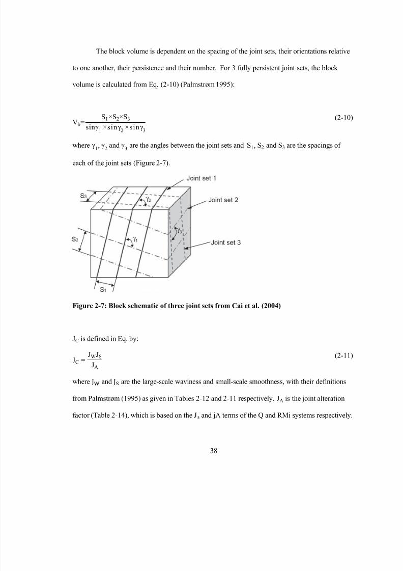
8/11/2019 Numerical Validation and Refinement of Empirical Rock Mass Modulus
http://slidepdf.com/reader/full/numerical-validation-and-refinement-of-empirical-rock-mass-modulus 58/263
The block volume is dependent on the spacing of the joint sets, their orientations relative
to one another, their persistence and their number. For 3 fully persistent joint sets, the block
volume is calculated from Eq. (2-10) (Palmstrøm 1995):
V bSSS3
sin
sin
sin3
(2-10)
where , and 3 are the angles between the joint sets and S, S and S3 are the spacings of
each of the joint sets (Figure 2-7).
Figure 2-7: Block schematic of three joint sets from Cai et al. (2004)

8/11/2019 Numerical Validation and Refinement of Empirical Rock Mass Modulus
http://slidepdf.com/reader/full/numerical-validation-and-refinement-of-empirical-rock-mass-modulus 59/263
Table 2-14: JA ratings from Cai et al. (2004)
Term Description JA
Rock Wall Contact
Clean joints
Healed or "welded" joints
(unweathered)
Softening, impermeable filling (quartz, epidote etc.) 0.75
Fresh rock walls (unweathered) No coating or filling on joint surface, except for staining 1
Alteration of joint wall: slightly
to moderately weathered
The joint surface exhibits one class higher alteration than the
rock
2
Alteration of joint wall: highly
weathered
The joint surface shows two classes higher alteration than the
rock
4
Coating or thin filling
Sand, silt, calcite etc. Coating of frictional materials without clay 3
Clay, chlorite, talc etc. Coating of softening and cohesive minerals 4
Filled joints with partial or no
contact between the rock wall
surfaces
Sand, silt, calcite, etc. Filling of frictional material without clay 4
Compacted clay materials "Hard" filling of softening and cohesive materials 6
Soft clay materials Medium to low over-consolidation of filling 8
Swelling clay materials Filling material exhibits swelling properties 8-12
2.2
Strength and Stiffness Parameter Estimation Methods Related to Tunnel
Convergence

8/11/2019 Numerical Validation and Refinement of Empirical Rock Mass Modulus
http://slidepdf.com/reader/full/numerical-validation-and-refinement-of-empirical-rock-mass-modulus 60/263

8/11/2019 Numerical Validation and Refinement of Empirical Rock Mass Modulus
http://slidepdf.com/reader/full/numerical-validation-and-refinement-of-empirical-rock-mass-modulus 61/263
Singh (2001) and Hoek & Diederichs (2006) as a reference to some of these relationships. A first
example is the relationship proposed by Serafim & Pereira (1983) from the RMR system and is
given by Eq. (2-16) in units of GPa, based on many results of cases of RMR < 50:
Erm RMR (2-16)
This relationship has a physical drawback in that it predicts a rock mass modulus higher
than intact stiffness for high RMR values. A second example, which a key component of this
research, is that given by Hoek & Diederichs (2006) on the basis of GSI. The Generalized Hoek-
Diederichs empirical relationship is based on a sigmoid function and is given by:
Erm Ei
eGS
(2-17)
where Ei is the intact Young’s Modulus and is the disturbance factor as described in Section
2.2.1.1.
2.2.3 Analytical Solutions to Problems in Rock Mechanics
Closed-form solution techniques to problems in rock mechanics are limited to simple materials
and in the case of underground excavations, simple excavation geometries. The analytical
solution techniques are those that form a mathematical relationship between the stresses and

8/11/2019 Numerical Validation and Refinement of Empirical Rock Mass Modulus
http://slidepdf.com/reader/full/numerical-validation-and-refinement-of-empirical-rock-mass-modulus 62/263
X and Y axes respectively and that σ > σ3 > , the solution to the state of stress around the
opening is given by in Eqs. (2-18), (2-19) and (2-20) (Jaeger et al. 2007):
σrr σσ3
a
r
σσ3
a
r
3 a
r cosθ
(2-18)
σθθ σσ3 a
r
σσ3 3 a
r
cos θ (2-19)
σrθ σσ3
a
r
3 a
r sinθ
(2-20)
where σrr is the stress normal to the circular boundary, σθθ is the stress tangent to the circular
boundary, σrθ is the shear stress acting normal to the plane of the thin plate and a and r are the
radius of the circular opening and radial distance from the centre respectively (Figure 2-8). The
radial inward convergence, Ur at any point along the boundary of the tunnel (r = a) can be found
from the following equation:
σθθ (2 21)

8/11/2019 Numerical Validation and Refinement of Empirical Rock Mass Modulus
http://slidepdf.com/reader/full/numerical-validation-and-refinement-of-empirical-rock-mass-modulus 63/263
Figure 2-8: Conceptual sketch of the circular opening in an infinite elastic medium
In the simple case for a hydrostatic stress field po σ
σ3 > , the mathematical
solutions to the stresses are given in Eqs. (2-22), (2-23) and (2-24):
a (2-22)
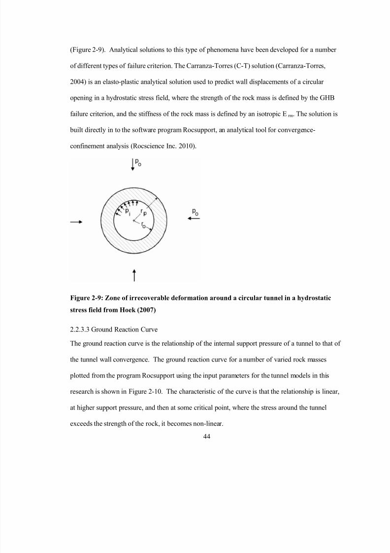
8/11/2019 Numerical Validation and Refinement of Empirical Rock Mass Modulus
http://slidepdf.com/reader/full/numerical-validation-and-refinement-of-empirical-rock-mass-modulus 64/263

8/11/2019 Numerical Validation and Refinement of Empirical Rock Mass Modulus
http://slidepdf.com/reader/full/numerical-validation-and-refinement-of-empirical-rock-mass-modulus 65/263
Figure 2-10: Ground reaction curve for rock masses at different values of GSI
2.3
Problem Statement
Faced with the problem of tunnel convergence, closed-form analytical tools are a useful means

8/11/2019 Numerical Validation and Refinement of Empirical Rock Mass Modulus
http://slidepdf.com/reader/full/numerical-validation-and-refinement-of-empirical-rock-mass-modulus 66/263
necessary to account for the effect of discontinuities in the overall rock mass behaviour. For this
reason, the Finite Element Method (FEM) numerical analysis, with the ability to explicitly
represent joints is used for this analysis.
2.4 References
Barton, N. (1976). Recent Experiences with the Q-System of Tunnel Support Design. Exploration
for rock engineering, proc. of the symp. 1, pp. 107-117. Cape Town: A.A. Balkema.
Barton, N. (2002). Some New Q-Value Correlations to Assist in Site Characterisation and Tunnel
Design. Int J Rock Mech Mining Sci, 39(2), 185-216.
Barton, N., Lien, R., & Lunde, J. (1974). Engineering Classification of Rock Masses for the
Design of Tunnel Support. Rock Mech, 6, 183-236.
Bieniawski, Z. (1973, Dec.). Engineering Classification of Jointed Rock Masses. The Civil
Engineer in South Africa, pp. 335-343.
Bieniawski, Z. (1976). Rock mass classifications in rock engineering. In Z. Bieniawski (Ed.),
Exploration for rock engineering, proc. of the symp. 1, pp. 97-106. Cape Town: A.A. Balkema.
Bieniawski, Z. (1978). Determining Rock Mass Deformability: Experience from Case Histories.
Int J Rock Mech Mining Sci & Geomechy Abstr, 15(5), 237-247.
Bieniawski, Z. (1989). Engineering Rock Mass Classifications. New York: Wiley.
Cai, M., Kaiser, P., Uno, H., Tasaka, Y., & Minami, M. (2004). Estimation of Rock Mass
Deformation Modulus and Strength of Jointed Hard Rock Masses using the GSI System. Int J
R k M h Mi i S i 41 3 19

8/11/2019 Numerical Validation and Refinement of Empirical Rock Mass Modulus
http://slidepdf.com/reader/full/numerical-validation-and-refinement-of-empirical-rock-mass-modulus 67/263
Hoek, E. (2007). Practical Rock Engineering.
Hoek, E. & Marinos, P. (2009). Tunnelling in Overstressed Rock. In I. Vrkljan (Ed.), Proc Eurock
Symp.
Hoek, E., & Diederichs, M. (2006). Empirical Estimation of Rock Mass Modulus. Int J Rock
Mech Mining Sci, 43(2), 203-215.
Hoek, E., & Marinos, P. (2000). GSI: A Geologically Friendly Tool for Rock Mass Strength
Estimation. Proc. GeoEng2000 Conference (pp. 1422-1446). Melbourne: Technomic publishers.
Hoek, E., Carranza-Torres, C., & Corkum, B. (2002). Hoek-Brown Failure Criterion - 2002Edition. In R. Hammah, W. Bawden, J. Curran, & M. Telesnicki (Ed.), proceedings of the 5th
North American Rock Mechanics Symposium and the 17th Tunnelling Association of Canada
Conference, NARMS-TAC 2002. Toronto: University of Toronto Press.
Hoek, E., Kaiser, P., & Bawden, W. (1995). Support of Underground Excavations in Hard Rock.
Rotterdam: Balkema.
Hoek, E., Marinos, P., & Marinos, V. (2005). Characterisation and Engineering Properties ofTectonically Undisturbed but Lithologically Varied Sedimentary Rock Masses. Int J Rock Mech
Mining Sci, 42, 277-285.
Jaeger, J., Cook, N., & Zimmerman, R. (2007). Fundamentals of Rock Mechanics (Fourth ed.).
Malden: Blackwell Publishing Ltd.
Marinos, V., Marinos, P., & Hoek, E. (2005). The geological strength index: applications and
limitations. Bull Eng Geol Environ, 64, 55-65.
Palmstrøm, A. (1982). The Volumetric Joint Count - A Useful and Simple Measurement of the
Degree of Rock Jointing Proc 4th Congress Int Assn Engineering Geology Delhi: 221 228

8/11/2019 Numerical Validation and Refinement of Empirical Rock Mass Modulus
http://slidepdf.com/reader/full/numerical-validation-and-refinement-of-empirical-rock-mass-modulus 68/263
Rocscience Inc. (2010). RocSupport Reference Documentation. Toronto, Ontario, Canada.
Serafim, J., & Pereira, J. (1983). Consideration of the Geomechanical Classification of
Bieniawski. Proc Int Symp Eng Geol Underground Construction, I, pp. 33-44.
Sonmez, H., & Ulusay, R. (1999). Modifications to the Geological Strength Index (GSI) and their
Applicability to Stability of Slopes. Int J Rock Mech Mining Sci, 36, 743-760.

8/11/2019 Numerical Validation and Refinement of Empirical Rock Mass Modulus
http://slidepdf.com/reader/full/numerical-validation-and-refinement-of-empirical-rock-mass-modulus 69/263
Chapter 3
The Finite Element Method in Numerical Analysis
3.1 Background
Closed-form methods for the calculation of stresses, displacements and failure of a rock mass
surrounding an underground excavation such as a tunnel become increasingly difficult with the
addition of complexity to the geometry and characteristics of the rock mass. The ability of most
Finite Element Method (FEM) solutions to model discontinuous, inhomogeneous, anisotropic and
non-elastic (DIANE) rock masses has made it a favorable choice for numerical analysis. In
addition to complex geometries, some FEM applications have the ability to explicitly represent
discontinuities within a rock mass, and incorporate their mechanical properties in to the numerical
solution of rock mass behaviour. FEM analysis is limited to simple behaviour and small
deformations, as it is not capable of capturing large deformations such as block detachment or
block rotation because of the requirement for the modelled rock mass or materials to be
continuous. Joints can be represented by special elements but small scale separation across the
joint is simulated by a reduction in the normal stiffness of the joint and not by actual

8/11/2019 Numerical Validation and Refinement of Empirical Rock Mass Modulus
http://slidepdf.com/reader/full/numerical-validation-and-refinement-of-empirical-rock-mass-modulus 70/263
interconnected by a fixed number of points (termed nodes) that store the values to the solution (or
approximated solution) of each given element (Figure 3-1). The assemblage of elements in the
domain is termed the mesh, of whose density plays a major role in the computation of the
solution.
Figure 3-1: FEM discretization of domain into triangular elements
The approximation to the solution of the PDE for each element is then made, by first
approximating the displacements over each element (ue) through a series of functions (the shape
functions, i) from the displacements at the nodes, as defined by the geometry of the element.
This formulation is expressed in Eq. (3-1), where M is the number of nodes in the element.
∑M (3-1)

8/11/2019 Numerical Validation and Refinement of Empirical Rock Mass Modulus
http://slidepdf.com/reader/full/numerical-validation-and-refinement-of-empirical-rock-mass-modulus 71/263
K e∫ BT
V
BdV (3-2)
Each element’s stiffness and displacements are assembled in a global system of
equilibrium equations of the form Ku = F, expressed in Eq. (3-3):
∑[K ije ]{u j
e}
i
∑f ie
i
(3-3)
where {u je} is the vector for the nodal value of displacements and f ie is the vector for body forces
and boundary conditions respectively. The displacements for all the nodes in the mesh are solved
for simultaneously by the evaluation of Eq. (3-3), from which the stresses and strains can be
evaluated. Most FEM software applications include both elastic and plastic models for the
relationship of the stresses and strains (Jing 2003, Pande et al. 1990).
3.2.1
Elasticity Models
The elastic model in FEM analysis is usually considered to be linear, for which the constitutive
relationship between the incremental stresses and incremental strains remain constant. At a basic
level, elastic properties can be considered as isotropic, meaning they do not vary with direction.

8/11/2019 Numerical Validation and Refinement of Empirical Rock Mass Modulus
http://slidepdf.com/reader/full/numerical-validation-and-refinement-of-empirical-rock-mass-modulus 72/263
Figure 3-2: Anisotropy of a rock mass. (Left) Orthotropic rock mass (Right) Transversely
isotropic rock mass.
The elasticity model used in this research, in so far as the modelled rock material goes, is
that of isotropy. The constitutive matrix of equation (3-2) above, for the 2-dimensional
plane-strain case, takes the general form:
Eνν ν ν
ν ν
ν
(3-4)
where E and ν are Young’s Modulus and Poisson’s Ratio respectively
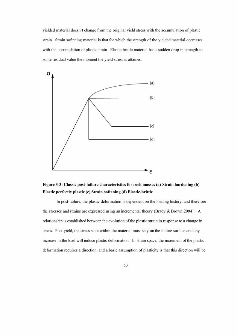
8/11/2019 Numerical Validation and Refinement of Empirical Rock Mass Modulus
http://slidepdf.com/reader/full/numerical-validation-and-refinement-of-empirical-rock-mass-modulus 73/263
yielded material doesn’t change from the original yield stress with the accumulation of plastic
strain. Strain softening material is that for which the strength of the yielded material decreases
with the accumulation of plastic strain. Elastic brittle material has a sudden drop in strength to
some residual value the moment the yield stress is attained.

8/11/2019 Numerical Validation and Refinement of Empirical Rock Mass Modulus
http://slidepdf.com/reader/full/numerical-validation-and-refinement-of-empirical-rock-mass-modulus 74/263
normal to a surface defined by the plastic potential function Q, which is a scalar function of
stresses. This is known as the flow rule, as given in Eq. (3-5):
{ε p} ̇ Q
σ (3-5)
where {ε p} ̇ is the plastic strain increment vector and is a non-negative constant of
proportionality that may vary over the load history. The flow rule is said to be associated if Q
F, and non-associated in the case where Q F. The plastic deformation may then change the
shape of or move the failure surface to a different stress state. A hardening or softening rule is
then required, to specify how the yield function changes with the addition of plastic strain (Pande
et al. 1990).
The goal of plasticity is to establish a relationship between the stresses and the total
strains, which is related by the elasto-plastic constitutive matrix [ep] for the consideration of
both the elastic and plastic strain. The derivation of the [ep] is made on the basis of the
additivity postulate in Eq. (3-6), which states that the total strain is a result of both the elastic and
plastic strain:
ε {ε p} εe (3-6)

8/11/2019 Numerical Validation and Refinement of Empirical Rock Mass Modulus
http://slidepdf.com/reader/full/numerical-validation-and-refinement-of-empirical-rock-mass-modulus 75/263
3.2.3
Discontinuity Representation in FEM
3.2.3.1 General
In the consideration of the FEM numerical representation of a rock mass, it is necessary to also
include the major discontinuities present and their contribution to the overall strength and
deformability, as they will dominate the behaviour of the rock mass. Some of the mechanical
properties of discontinuities, which are relevant to this research, include (Goodman et al. 1968):
- They have little or no resistance to a net tension force
- They have some deformability in the normal direction, but high resistance in compression
- Under high confining pressures the shear strength is governed by the strength properties
of the asperities as the adjacent walls shear through them
- They can deform in shear, at shear stresses below the shear strength
3.2.3.2
Joint Stiffness
One such major development to incorporating the joint element mathematically into FEM
analysis is the well-known four-node line element of zero thickness of length L (Figure 3-4),
alternatively termed the "Goodman Joint Element" (Jing 2003). The constitutive model follows a
linear relationship, where the elastic properties are expressed in terms of joint normal (K n) and

8/11/2019 Numerical Validation and Refinement of Empirical Rock Mass Modulus
http://slidepdf.com/reader/full/numerical-validation-and-refinement-of-empirical-rock-mass-modulus 76/263
Figure 3-4: Four-noded "Goodman Joint Element" after Goodman et al. (1968)
The node pairs (1,4) and (2,3) initially have identical coordinates in the local coordinate
system. The vector w is the relative displacement of the top segment to the bottom segment of
the element, given in Eq. (3-7):
w ws
wn ws
topws
bottom
wntop
wn bottom
(3-7)
K n and K s are then used to relate the vector of forces P to the relative displacement vector using
the constitutive relationship of Eq. (3-8):
P K s K n ws
wn (3-8)

8/11/2019 Numerical Validation and Refinement of Empirical Rock Mass Modulus
http://slidepdf.com/reader/full/numerical-validation-and-refinement-of-empirical-rock-mass-modulus 77/263
whose non-zero terms are each expressed as a function of K n and K s. The local joint element
stiffness is then assembled to the global finite element stiffness matrix.
The K n and K s parameters in this research for FEM analysis are constants, meaning their
values do not change as a function of stress. In reality, it has been observed that both parameters
will follow a non-linear loading path, as demonstrated by Bandis et al. (1983). Figure 3-5 shows
the different components of the normal stress vs. closure and shear stress vs. shear displacement
in terms of the initial normal stiffness (K ni), the initial shear stiffness (K si), the tangent K n and K s,
and the secant normal stiffness (K n,secant) and secant peak shear stiffness (K s,secant (peak)) for a
discontinuity. As convention in this research, the terms K n and K s used throughout, refer to the
secant normal and secant peak shear stiffness respectively as defined on these curves.

8/11/2019 Numerical Validation and Refinement of Empirical Rock Mass Modulus
http://slidepdf.com/reader/full/numerical-validation-and-refinement-of-empirical-rock-mass-modulus 78/263
displacements (Kulhawy 1975). This lab method, as well as using triaxial compression testing,
have been demonstrated and compared to in situ tests by Rosso (1976). In the event where in situ
loading test data is unavailable, Barton (1972) gave an empirical relationship for the estimation of
K n for one joint set on the basis of known values for Ei, Erm and the spacing of the joints (L) in
Eq. (3-10):
Erm
Ei
K n
K nEi
(3-10)
The equation assumes the loading is perpendicular to the joint set. By similar analogy for
K s, if values are known for the intact shear modulus of rock (Gi) and the shear modulus of the
rock mass (Grm), then it may be estimated from Eq. (3-11), which is after Karzulovic, et al.
(2009):
K s GrmGi
GiGrm (3-11)
Another relationship as provided by Kulhawy (1975), assuming the stiffness of the
discontinuity is related directly to equivalent elastic parameters, K s is related to K n empirically
using Eq. (3-12):
K s K n
(3-12)

8/11/2019 Numerical Validation and Refinement of Empirical Rock Mass Modulus
http://slidepdf.com/reader/full/numerical-validation-and-refinement-of-empirical-rock-mass-modulus 79/263
In the consideration of a natural joint surface in situ, it is never as smooth as the
conditions of laboratory testing used for the determination of ϕ. One major issue with the Mohr-
Coulomb failure criterion is that ϕ depends on σn, as observation of natural discontinuities show a
curved failure envelope. At low values of σn along rough joint surfaces, the shear displacement
will occur in response to one block riding up along the asperities of the other, resulting in a value
for ϕ to be greater and leading to dilation. At some point when the value of σn is high enough,
shearing will begin to occur through the asperities of the intact rock, reducing ϕ to the angle of
friction of the intact rock (Figure 3-6).
Figure 3-6: Block sketches of joint behaviour, under (Left) low normal stress leading to

8/11/2019 Numerical Validation and Refinement of Empirical Rock Mass Modulus
http://slidepdf.com/reader/full/numerical-validation-and-refinement-of-empirical-rock-mass-modulus 80/263
Each of the parameters is obtained from established field testing methods and is
independent of σn The field estimation for R can be done using a carpenter’s comb on the
joint surface, and comparing it with the 10cm scale profile shown in Figure 3-7. Field
estimations for JCS can be made using a Schmidt hammer to the exposed joint wall and
converting the index value to compressive strength. ϕr is obtained empirically from residual tilt
tests following the methodology described in (Barton & Choubey 1977).
The Barton-Bandis criterion is limited to discontinuities of geological origin, meaning the
formulation does not apply to rock joints where there is significant infill preventing direct
rock/rock contact of the rock walls. The reasoning provided by the authors in the original
formulation is that the mechanical behaviour of the joint will be governed by the filling material,
and therefore requires specialized and separate formulations (Barton 1973, Barton & Choubey
1977).

8/11/2019 Numerical Validation and Refinement of Empirical Rock Mass Modulus
http://slidepdf.com/reader/full/numerical-validation-and-refinement-of-empirical-rock-mass-modulus 81/263

8/11/2019 Numerical Validation and Refinement of Empirical Rock Mass Modulus
http://slidepdf.com/reader/full/numerical-validation-and-refinement-of-empirical-rock-mass-modulus 82/263
3.3
Tunnel Advance Modelling in Plane-Strain FEM
3.3.1
General
The excavation of a tunnel within a rock mass forms a complex influence on the stress regime
and internal displacements associated with the boundary of the tunnel in 3 dimensions. The
advancing face of the tunnel will provide an inherent support for the excavation initially, which is
known as the apparent support pressure. This is gradually reduced as the face advances. It has
been observed that deformation as a result of tunnel excavation occurs in the rock mass 1/2 of the
tunnel diameter distance ahead of the face, is 1/3 of the total closure at the face itself and is at a
maximum level at a distance of 1 ½ diameters behind the face (Hoek 1998). Two common
methods for the 2-dimensional FEM plane-strain simulation of this process are the material
softening method and the field stress vector or average pressure reduction method.
3.3.2
Material Softening Method
The material softening method (Figure 3-8) emulates the advance of a tunnel, by successively
replacing the tunnel face in the FEM model with a de-stressed, softer material and allowing the

8/11/2019 Numerical Validation and Refinement of Empirical Rock Mass Modulus
http://slidepdf.com/reader/full/numerical-validation-and-refinement-of-empirical-rock-mass-modulus 83/263

8/11/2019 Numerical Validation and Refinement of Empirical Rock Mass Modulus
http://slidepdf.com/reader/full/numerical-validation-and-refinement-of-empirical-rock-mass-modulus 84/263
hydrostatic, surface tractions along the boundary of the excavation must be calculated and applied
to each boundary element of the excavation, such that it is opposite in direction to the associated
field stress tractions acting on that element.

8/11/2019 Numerical Validation and Refinement of Empirical Rock Mass Modulus
http://slidepdf.com/reader/full/numerical-validation-and-refinement-of-empirical-rock-mass-modulus 85/263
3.3.4
Longitudinal Displacement Profile
While the concept of a plane-strain simulation for tunnel advance discussed in the previous two
sections is important, in order to have any practical meaning in tunnel support design it is
necessary to correlate the associated tunnel wall deformations and internal pressures to an actual
physical location along the tunnel axis away from the face (Vlachopoulos & Diederichs 2009).
The longitudinal displacement profile (LDP) is a method for calibrating this relationship, which is
an equation relating the tunnel wall closure to the distance from the tunnel face, as shown
graphically in Figure 3-10.

8/11/2019 Numerical Validation and Refinement of Empirical Rock Mass Modulus
http://slidepdf.com/reader/full/numerical-validation-and-refinement-of-empirical-rock-mass-modulus 86/263
tunnel as well as the current and maximum tunnel wall displacement. The latter three can be
determined from simple plane-strain FEM numerical analysis.
3.4 Phase2 Finite Element Analysis
Phase2 is a 2-dimensional, elasto-plastic FEM program used for the analysis of complex problems
in both rock and soil mechanics. A number of constitutive models for materials and joints, and
some support types and groundwater models are built-in to version 7. All constitutive models
used for this research are built in to the software directly. The analysis of 2-dimensional
problems is either performed under plane-strain or axisymmetric conditions (Rocscience Inc.
2010).
A key element of the program is the ability to specify joint sets to the model via the joint
network functionality. The sets can be generated over 2 dimensions using a number of statistical
or deterministic means. This functionality has been the major contributing factor to the selection
of Phase2 for the modelling used in this research. The emulation of the "Goodman joint element",
specifically for the densest of joint models in this research, required a significant amount of
processing and computer resources for the initial model construction and computation. While it
was possible to mesh and solve these models, post-processing was not possible or was

8/11/2019 Numerical Validation and Refinement of Empirical Rock Mass Modulus
http://slidepdf.com/reader/full/numerical-validation-and-refinement-of-empirical-rock-mass-modulus 87/263
tunnel to be equal in magnitude and opposite in direction to the field stress acting on the
boundary (Rocscience Inc., 2010).
3.5 References
Bandis, S., Lumsden, A., & Barton, N. (1983). Fundamentals of Rock Joint Deformation. Int J
Rock Mech Mining Sci & Geomech Abstr, 20(6), 249-268.
Barton, N. (1972). A Model Study of Rock-Joint Deformation. Int J Rock Mech Mining Sci &
Geomech Abstr, 9, 579-602.
Barton, N. (1973). Review of a New Shear-Strength Criterion for Rock Joints. Eng Geol, 7(4),
287-332.
Barton, N. (1976). The Shear Strength of Rock and Rock Joints. Int J Rock Mech Mining Sci &
Geomech Abstr, 13(9), 255-279.
Barton, N., & Bandis, S. (1990). Review of Predictive Capabilities of JRC-JCS Model in
Engineering Practice. In N. Barton, & O. Stephansson (Ed.), Rock joints, Proc Int Symp on RockJoints, Loen, Norway (pp. 603-610). Rotterdam: A.A. Balkema.
Barton, N., & Choubey, V. (1977). The Shear Strength of Rock Joints in Theory and Practice.
Rock Mech Rock Eng, 10(1), 1-54.
Brady, B., & Brown, E. (2004). Rock Mechanics for Underground Mining. Dordrecht: Kluwer
Academic Publishers.
Goodman, R., Taylor, R., & Brekke, L. (1968). A Model for the Mechanics of Jointed Rock.
ASCE Journal of the Soil Mech and Found Div, 94(SM3), 637-659.

8/11/2019 Numerical Validation and Refinement of Empirical Rock Mass Modulus
http://slidepdf.com/reader/full/numerical-validation-and-refinement-of-empirical-rock-mass-modulus 88/263
Kulhawy, F. (1975). Stress Deformation Properties of Rock and Rock Discontinuities. Eng Geol,
9, 327-350.
Pande, G., Beer, G., & Williams, J. (1990). Numerical Methods in Rock Mechanics. Chichester,England: John Wiley & Sons Ltd.
Rocscience Inc. (2010). RocSupport reference documentation. Toronto, Ontario, Canada.
Rosso, R. (1976). A Comparison of Joint Stiffness Measurements in Direct Shear, Triaxial
Compression, and In Situ. Int J Rock Mech Mining Sci & Geomech Abstr, 13(6), 167-172.
Vlachopoulos, N. (2009). Back Analysis of a Tunnelling Case Study in Weak Rock of the Alpine
System in Northern Greece: Validation and Optimization of Design Analysis based on Ground
Characterization and Numerical Simulation. PhD. Thesis, Queen's University, Kingston.
Vlachopoulos, N., & Diederichs, M. (2009). Improved Longitudinal Displacement Profiles for
Convergence Confinement Analysis of Deep Tunnels. Rock Mech Rock Eng, 42(2), 131-146.

8/11/2019 Numerical Validation and Refinement of Empirical Rock Mass Modulus
http://slidepdf.com/reader/full/numerical-validation-and-refinement-of-empirical-rock-mass-modulus 89/263
Chapter 4
Numerical Modelling Method
For the numerical modelling verification of the Generalized Hoek-Diederichs empirical
relationship specific to tunnelling, a suite of models was constructed with the goal of comparing
the deformations in models with an explicit representation of joints, to continuum models where
the deformational characteristics of the joints and intact rock between them are represented by
Erm. The modelling analysis consists of two stages.
The first stage was the development of block models that resemble a standard unconfined
compressive strength (UCS) test, which was used to calibrate the parameters of the joints and
their structure (the spacing and number of discontinuity sets) used throughout the modelling
analysis. The calibration was performed by initially estimating the elastic K n and K s values for
the joints on the basis of their contribution to deformation in addition to Ei, and from the back-
calculation of an associated Erm from the displacements and stresses obtained in the model. A
framework is provided for the GSI characterization of the jointed model pertaining to the
discontinuity structure and surface conditions. Additional block models were run with inelastic

8/11/2019 Numerical Validation and Refinement of Empirical Rock Mass Modulus
http://slidepdf.com/reader/full/numerical-validation-and-refinement-of-empirical-rock-mass-modulus 90/263
over 3 different depths in order to evaluate the methodology in different strength and stress
regimes. The models were first run completely elastically, then run with perfectly plastic intact
rock and elastic joints, and run with perfectly plastic intact rock and inelastic joints. The purpose
of including inelastic joints in this stage as well as in the block models is to answer the question
as to whether slip along the joints is a deformation contribution included when Erm is estimated
using the Hoek-Diederichs method.
The two phases of the research are shown conceptually with respect to the typical stress-
strain curve of a rock mass undergoing loading and subsequent unloading in Figure 4-1. As the
calibration of the joints uses an estimated Erm in the form of block models where compressional
testing is performed (loading), and tunnel excavations create stress relief of the surrounding rock
mass, it is assumed that (4) and (3) in Figure 4-1 are identical.
4.1 Finite Element Analysis using Phase2
The software program Phase2 includes the "Goodman joint element", and Version 7 includes a
joint networking feature. This feature has the distinct advantage of providing the ability to
specify a 2-dimensional system of joints. Numerous deterministic and probabilistic algorithms
are available for the generation of the joint networks. The simplicity and efficiency of the

8/11/2019 Numerical Validation and Refinement of Empirical Rock Mass Modulus
http://slidepdf.com/reader/full/numerical-validation-and-refinement-of-empirical-rock-mass-modulus 91/263
Figure 4-1: Stress-Strain curve of a rock mass undergoing loading and subsequent
unloading - (1) Initial tangent modulus (2) elastic tangent modulus (3) Recovery modulus (4)
Erm from Hoek & Diederichs (2006).
The scope of this research is the numerical modelling of tunnels at significant depth.
This is considered to be a high compressional stress regime, in which the individual rock blocks

8/11/2019 Numerical Validation and Refinement of Empirical Rock Mass Modulus
http://slidepdf.com/reader/full/numerical-validation-and-refinement-of-empirical-rock-mass-modulus 92/263
which impede the accomplishment of this goal that include the scope of research and computer
resource limitations. As such, the term "modelling GSI spectrum", as is commonly referred to in
this thesis, is a subset of the general GSI chart (Figure 2-5) where the structure ranges from
"Intact or Massive" through to "Blocky/Disturbed/Seamy", and the surface conditions range from
"Very Good" through to "Very Poor".
4.2.1
Computer Resource Limitations
The Phase2 FEM program has been designed to run in a 32-bit processing environment. As a
consequence, the application is only capable of addressing, at most, 32 bits of memory space (232
bytes or 4GB), and is further reduced by as much as half of this because of the host operating
system requirements. In general terms, this means there is a theoretical limit on the size of the
model in terms of the number of elements and the degrees of freedom that can be analyzed using
this FEM code. This limitation has been observed when constructing the models for this
research, when increasing the joint density with respect to the equivalent structure in GSI. Within
Phase2 during the pre-processing phase (meshing), program instabilities were observed as the
memory requirements approached this theoretical limit. In order to address this issue, the tunnel
models were prepared by taking advantage of the symmetry of the jointed rock mass for each of

8/11/2019 Numerical Validation and Refinement of Empirical Rock Mass Modulus
http://slidepdf.com/reader/full/numerical-validation-and-refinement-of-empirical-rock-mass-modulus 93/263
memory limitations. As a result, a Microsoft® Excel® macro was programmed in order to obtain
specific data from the computed data files, for both the block and tunnel models. The source
code of this macro can be found in Appendix B. In reference to the block model shown in Figure
4-2 (left), the process for back-calculating Erm is as follows, for each stage in the model:
1. Interpolate the vertical displacements for n points along lines L1 and L2, and take the
average across each line Δdavg,L1 and Δdavg,L2)
2.
Obtain the strain by subtracting Δdavg,L2 from Δdavg,L1
3. Interpolate and average the vertical stress from points across the top line located just
above the boundary of the jointed rock mass
4. Display the results into a spreadsheet to calculate Erm for each stage
8/11/2019 Numerical Validation and Refinement of Empirical Rock Mass Modulus
http://slidepdf.com/reader/full/numerical-validation-and-refinement-of-empirical-rock-mass-modulus 94/263
Tunnel closure was also calculated via the macro for each stage of the excavation in the
tunnel models shown in Figure 4-2 (right), by finding all nodes and their associated total
displacements along the tunnel boundary and calculating their average.
4.2.2 Isotropy and Anisotropy
As was stated in Chapter 2, Erm estimation from the output of rock mass classification systems
assumes isotropic rock mass conditions. On the basis of the diagrams as provided in GSI, it is
clear that a rock mass whose structure is considered to be "Laminated/Sheared" will exhibit an
anisotropic response under load, at the scale of the tunnel application. Conditions that are highly
anisotropic, such as laminated ground, are considered to be a separate issue and are therefore
excluded from this research.
4.3 Numerical Model Representation of the Modelling GSI Spectrum
The methodology for representing a model equivalent within the modelling GSI spectrum
combines the input parameter quantification of the GSI system proposed by Cai, et al. (2004)
with the descriptions of the original GSI system from Hoek, et al. (2000). The degree of
blockyness, or structure of a rock mass, is determined based on the number of joint sets present
d h i i i l i h Th l i d h f h j i

8/11/2019 Numerical Validation and Refinement of Empirical Rock Mass Modulus
http://slidepdf.com/reader/full/numerical-validation-and-refinement-of-empirical-rock-mass-modulus 95/263
interlocking of rock pieces in the GSI system is represented numerically by increasing the number
of joint sets within the models, and/or decreasing the individual spacing of each joint set while
maintaining isotropy in the resulting rock mass.
The selection for the spacing of the joint sets was chosen so that the effective spacing of
all joint sets within the given model follows within the range suggested by Cai et al. (2004) for
spacing and block volume. The descriptions in both Cai et al. (2004) and Hoek & Marinos
(2000) for the rock mass structure are in terms of a 3-dimensional rock mass. However, the
analysis using Phase2 is a 2-dimensional plane-strain representation, and therefore this is
accommodated by assuming that one joint set is oriented parallel to the plane of representation,
with its spacing normal to this plane. Each of the four numerical representations of structure over
the modelling GSI spectrum is shown in Figures 4-3 and 4-4.

8/11/2019 Numerical Validation and Refinement of Empirical Rock Mass Modulus
http://slidepdf.com/reader/full/numerical-validation-and-refinement-of-empirical-rock-mass-modulus 96/263
Figure 4-4: Numerical representation of: (Left) Very Blocky rock mass – 3 joint sets with
0.5m spacing (Right) Blocky/Disturbed/Seamy rock mass – 4 joint sets with 0.3m spacing
4.4 Modelling Input Parameters
Chapter 2 presents a comprehensive review of rock mass classification systems, and how they can
be used for parameter estimation in finite element numerical analysis. The following section
details the assumptions made and the methodology used for the derivation of the key numerical
inputs used for this research. Each of the input parameters for stiffness and strength in this

8/11/2019 Numerical Validation and Refinement of Empirical Rock Mass Modulus
http://slidepdf.com/reader/full/numerical-validation-and-refinement-of-empirical-rock-mass-modulus 97/263
intact rock kept constant. In this sense the strength contribution to the displacements and stresses
found within the numerical analysis performed can be controlled, to further observe the stiffness
contribution.
4.4.1 Stiffness Parameters
4.4.1.1
Intact Rock
The methodology for the determination of the stiffness parameters defined in this section is
applicable to both the block and tunnel modelling analysis. For the Phase2 FEM analysis, the
intact rock is assumed to be isotropic, and therefore stiffness is represented by the Young’s
Modulus (Ei and Poisson’s ratio ) elastic properties of the rock material.
On the basis of the given rock type for each model, E i is estimated using σci and the
associated modulus ratio (MR) for the rock, using the following equation (Deere 1968, Hoek &
Diederichs 2006):
Ei MR σci (4-1)
Using the previously defined values for σci, the MR values were chosen along the same
lines as the engineering classification of intact rock on the basis of modulus ratio (Deere 1968).
T l t id f k hi h MR i i d t hi h t th k

8/11/2019 Numerical Validation and Refinement of Empirical Rock Mass Modulus
http://slidepdf.com/reader/full/numerical-validation-and-refinement-of-empirical-rock-mass-modulus 98/263
Table 4-1: Elastic properties for intact rock used in the Block and Tunnel Models
Block Models
MR Ei (MPa)
425 72250 0.25
Tunnel Models
Rock Strength MR Ei (MPa)
High 425 72250 0.25
Medium 250 18750 0.25
Low 100 2500 0.25
4.4.1.2
Discontinuities
As was described in Section 3.2.3.2, the joints in Phase2 are represented numerically as the
"Goodman joint element", where each element is defined in terms of a linear normal (K n) and
shear stiffness (K s) in accordance with the convention outlined in Section 3.2.3.2. Over the
modelling GSI spectrum, the representative values assumed for these properties will change as
the quality of the surface conditions of the discontinuities change. This has been the approach
applied to this study. The majority of the test data for the formulation of the Generalized Hoek-
Diederichs empirical relationship was derived in rock masses of GSI values ranging from 40-80

8/11/2019 Numerical Validation and Refinement of Empirical Rock Mass Modulus
http://slidepdf.com/reader/full/numerical-validation-and-refinement-of-empirical-rock-mass-modulus 99/263
quality of the rock masses for "Very Blocky" and "Blocky/Disturbed/Seamy". The resulting K n
and K s parameters used for all models are summarized in Table 4-2.
Figure 4-5: Fixed structure and varying surface conditions of GSI for K n and K s calibration
after Marinos et al. (2005)
Table 4 2: K and K values for varying surface conditions in models

8/11/2019 Numerical Validation and Refinement of Empirical Rock Mass Modulus
http://slidepdf.com/reader/full/numerical-validation-and-refinement-of-empirical-rock-mass-modulus 100/263
The empirical equation as given in Eq. (3-10) is generalized for n-joint sets of equal
spacing L, each oriented at some angle i with respect to the normal to the load applied. A
schematic for the i-th joint set is shown in Figure 4-6.

8/11/2019 Numerical Validation and Refinement of Empirical Rock Mass Modulus
http://slidepdf.com/reader/full/numerical-validation-and-refinement-of-empirical-rock-mass-modulus 101/263
K n E j σ
ε j
d
d
(4-3)
where F is the force normal to the joint set, A is the area of the joint and L is the spacing of the
joint set. ε j and d are the strain and total displacement over each joint in the joint set
respectively. Rearranging Eq. (4-3) to solve for the displacements in terms of F and K n, Eq. (4-4)
is then:
d K n
(4-4)
If the joint set is oriented at some angle with respect to the normal to the force F
(Figure 4-6), then the resulting displacement in the direction of the force becomes:
d n
K ncos
s
K s s in
cos
cosK n
cos
sin
cosK s
sin (4-5)
where ncos is the component of the force normal to the joint acting in the direction of F,
ssin is the component of the force tangent to the joint acting in the direction of F, and is the
area of the joint oriented at an angle . Substituting Eq. (4-5) into the total displacement term of
Eq. (4-3), and adjusting the spacing L to L' along the direction of the force F (Figure 4-6), the
rightmost term of Eq (4 2) can then be expressed in terms of both K and K (Eq (4 6)):

8/11/2019 Numerical Validation and Refinement of Empirical Rock Mass Modulus
http://slidepdf.com/reader/full/numerical-validation-and-refinement-of-empirical-rock-mass-modulus 102/263
Erm
Ei
cos cos K n
sin
K s
(4-7)
In order to generalize Eq. (4-7) for n-joint sets, let Jv be the volumetric joint count, which
is the sum of the number of joints per meter for all of the joint sets. This is shown in Eq. (4-8) to
be a summation of the inverse of the spacing for each joint set:
v
n
(4-8)
If Jv is the volumetric joint count, then 1/Jv = Le is the effective spacing for n-joint sets.
The accommodation for the effective spacing Le in Eq. (4-7) therefore results in Eq. (4-9), a
generalization of Eq. (3-10) for n-joint sets of equal spacing L, each oriented at some angle i
with respect to the normal to the load applied.
Erm
Ei
∑ cos i
cos iK ni
sin
iK si
n
i
(4-9)
Eq. (4-9) has been derived under the condition of isotropy, therefore each joint set is
assumed to have the same K n and K s values. The estimation of K n can then be expressed by
rearranging Eq. (4-9), and assuming that the values for Erm, Ei, , and K s are known.
h d lli l i i i d h h l i i f h di i i i

8/11/2019 Numerical Validation and Refinement of Empirical Rock Mass Modulus
http://slidepdf.com/reader/full/numerical-validation-and-refinement-of-empirical-rock-mass-modulus 103/263
different values for ν based on the degree of infill used in the relationship defined in Eq. (3-12).
They are based on reasonable values found in literature for the ranges given for infill materials
such as chlorite, talc, kaolinite and gypsum (Gercek 2007, Jackson et al. 1995, Wang et al. 2001,
Lama & Vutukuri 1978).
Table 4-3: Values for ν based on joint surface conditions used for the relationship between
K n and K s
Structure
Very Good, Good and Fair 0.25
Poor 0.30
Very Poor 0.35
The empirical estimation of
is then made by the substitution of Eq. (3-12) into Eq. (4-9), and
rearranging to form Eq. (4-10):
K n ErmEi
EiErm
∑cos i cos i sin
i νi
n
i
(4-10)
On the basis of GSI structure from "Intact or Massive" to "Blocky/Disturbed/Seamy", the
descriptions for the number of joint sets apply to a three-dimensional rock mass. It can be shown

8/11/2019 Numerical Validation and Refinement of Empirical Rock Mass Modulus
http://slidepdf.com/reader/full/numerical-validation-and-refinement-of-empirical-rock-mass-modulus 104/263
to use in the estimation of Erm from the Generalized Hoek-Diederichs empirical relationship as
given in Eq. (2-17). The disturbance factor D is assumed to be 0 in this case. This assumption is
possible because the research is focused on tunnelling applications where minimal disturbance is
expected to the rock during the excavation process. The values for GSI and Erm are summarized
in Tables 4-4 and 4-5, for the modelling GSI spectrum.
Table 4-4: Representative GSI for models over the modelling GSI spectrum
Very Good Good Fair Poor Very Poor
Intact 90 80 70 N/A N/A
Blocky 75 65 55 45 35
Very Blocky 65 55 45 35 25
Blocky/Disturbed/Seamy 55 45 35 25 15
Table 4-5: Representative Erm for models over the modelling GSI spectrum
Very Good Good Fair Poor Very Poor
Intact 69300 63600 52900 N/A N/A
Blocky 59000 45600 29500 16200 8200
Very Blocky 45600 29500 16200 8200 4300
Blocky/Disturbed/Seamy 29500 16200 8200 4300 2600
4.4.2
Strength Parameters

8/11/2019 Numerical Validation and Refinement of Empirical Rock Mass Modulus
http://slidepdf.com/reader/full/numerical-validation-and-refinement-of-empirical-rock-mass-modulus 105/263
separate value for mi and σci. The strength parameters given are assumptions of reasonable
values for the different rock types, as has been reported in literature (Hoek & Brown 1997, Hoek
& Marinos 2000).
Table 4-6 - Strength parameters for intact rock used in the block and tunnel models
Block Models
Strength Criterion
Generalized Hoek-
Brown
Peak Residual
ci
170 MPa
mi
29
mb
24
s
0.57
a
0.5
Dilation
0
mb
24
s
0.57
a
0.5
Tunnel Models
Strength Criterion
Generalized Hoek-
Brown
High Strength
Peak Residual
ci
170 MPa
mi
29
mb
24
s
0.57
a
0.5
Dilation
0
mb
24
s
0.57
a
0.5
Medium Strength
Peak Residual
ci
75 MPa
mi
17
mb
14
s
0.57
a
0.5
Dilation
0
mb
14
s
0.57
a
0.5

8/11/2019 Numerical Validation and Refinement of Empirical Rock Mass Modulus
http://slidepdf.com/reader/full/numerical-validation-and-refinement-of-empirical-rock-mass-modulus 106/263
given for surface conditions of the general GSI chart (Figure 2-5), and are within ranges to meet
the input parameter quantification for surface conditions used by Cai et al. (2004). As the
definitions and ratings for the terms W, S and in Eq. (2-11) are based on the ratings for the Q
and RMi systems, the relationships between these parameters and JRC, JCS and ϕr can be made.
For the JRC parameter, the term jwjs in Eq. (2-11) is equivalent to jR of the RMi system, which
is similar to Jr of the Q-system. Barton & Bandis (1990) reproduced a table (Figure 4-7) relating
Jr of the Q-system to JRC.
The JCS parameter is based on a combination of the degree of alteration interpreted from
definitions given surface conditions in the general GSI chart (Figure 2-5), and the jA/Ja terms of
the RMi and Q-systems respectively. As the strength of the joint walls is also dependent on the
strength of the intact rock, for the tunnel models JCS also varies with respect to the strength of
the intact rock. ϕr has been chosen to be within the ranges as suggested by Barton et. al. (1974)
given in Table 2-6. For all block and tunnel models for which the joint strength is defined by the
Barton-Bandis shear strength criterion, the strength parameters of the joints based on the GSI
surface conditions are given in Table 4-7.

8/11/2019 Numerical Validation and Refinement of Empirical Rock Mass Modulus
http://slidepdf.com/reader/full/numerical-validation-and-refinement-of-empirical-rock-mass-modulus 107/263
Figure 4-7: Relationship between Jr of the Q-System and JRC for 20cm and 1m samples
from Hoek et al. (1995)
Table 4-7: Joint shear strength parameters used in the block and tunnel models
Block models
Joint Surface Condition from GSI
Barton-Bandis Joint Shear Strength
Parameter
Very
GoodGood Fair Poor
Very
Poor

8/11/2019 Numerical Validation and Refinement of Empirical Rock Mass Modulus
http://slidepdf.com/reader/full/numerical-validation-and-refinement-of-empirical-rock-mass-modulus 108/263
4.4.2.3 Equivalent Rock Mass as a Continuum
The equivalent rock mass strength for the continuum based model is obtained by the estimation of
the GHB parameters from GSI, using the formulations provided in Section 2.2.1 along with the
GSI obtained from the characterization of the degree of blockyness and surface conditions for the
equivalent jointed models. The disturbance factor D is also assumed to be 0 as the intent of the
analysis is for simulation of a rock mass where minimal disturbance is expected to occur from the
excavation process. The rock mass strength is only applicable to those continuum models being
run plastically.
4.5 Block Models
4.5.1 General
The purpose of the construction of the block models is to calibrate the material and joint
parameters used for the tunnel modelling comparisons. Each model is set up in the form of a
UCS test, where a load is applied to the top of the model in the form of fixed displacements. The
theory behind this type of calibration is to determine the appropriate kinetics of the jointed
models under compression, in a simulated massive UCS test. The concept of the block model is
illustrated in Figure 4-8, and consists of the jointed rock mass between an elastic top and bottom

8/11/2019 Numerical Validation and Refinement of Empirical Rock Mass Modulus
http://slidepdf.com/reader/full/numerical-validation-and-refinement-of-empirical-rock-mass-modulus 109/263
Figure 4-8: Sample block model geometry used in the block model analysis
4.5.2 Boundary Conditions
Load has been applied in the form of fixed vertical node displacements along the top of each of
the block models Each model has been defined a specific load in order to ensure numerical

8/11/2019 Numerical Validation and Refinement of Empirical Rock Mass Modulus
http://slidepdf.com/reader/full/numerical-validation-and-refinement-of-empirical-rock-mass-modulus 110/263
amount Δdnv), the formula for Erm in basic terms of stress and strain in Eq. (4-11) is used as
follows:
Erm σ
ε (4-11)
where ε is the strain in the model in the vertical direction, given by Eq. (4-12):
ε dnv
dv
(4-12)
where dv is the total distance from the top of the model to the bottom of the model. Substituting
Eq. (4-12) into Eq. (4-11) and rearranging to solve for Δdnv:
dnv σ
Erm
dv (4-13)
The estimation of the stress was made by plotting the Barton-Bandis failure criterion in
shear stress vs. normal stress space, using the associated JRC, JCS and ϕr values for the "Very
Good" through to "Very Poor" surface conditions (Figure 4-9). Each joint set in the model was
then plotted using the origin of planes technique, where a line is plotted from the point equal to
the confinement stress of 0.1 MPa on the normal stress axis at an angle equal to the angle with
respect to the horizontal (counter-clockwise positive) of the joint set. The Mohr-Circle for the
stress state was then plotted such that the intersection of this circle with the least favourably

8/11/2019 Numerical Validation and Refinement of Empirical Rock Mass Modulus
http://slidepdf.com/reader/full/numerical-validation-and-refinement-of-empirical-rock-mass-modulus 111/263
Figure 4-9: Barton-Bandis strength criterion in τ – n space, with joint planes for joints in
model and Mohr circles for appropriate stress states
4 5 2 1 E t l B d i

8/11/2019 Numerical Validation and Refinement of Empirical Rock Mass Modulus
http://slidepdf.com/reader/full/numerical-validation-and-refinement-of-empirical-rock-mass-modulus 112/263
4.5.3
Joints
With the exception of the "Intact/Massive" structure models, all joint sets are fully persistent with
a varying degree of spacing, following the descriptions as shown in Figures 4-3 and 4-4. At the
intersection point between a joint and a boundary (joint or external boundary), the ends are
"open" in Phase2, meaning that it is represented by two nodes, which are free to move with
respect to each other. In the non-persistent "Intact/Massive" model, only the joint ends that
terminate within the rock mass are "closed", meaning that it is represented by one node, and
therefore relative movement cannot occur (Rocscience Inc. 2010).
4.5.4
Sensitivity Analysis
The goal of model sensitivity analysis is to determine the components of the model when varied
have influence on the results of the model. Varying every component of the numerical model and
a combination of each is impractical and unnecessary. By way of example in this study, the
sensitivity to the scale of a block model needs only to be demonstrated for one model within the
modelling GSI spectrum, i.e. a model with "Very Blocky" structure and "Fair" joint surface
conditions. It is assumed that the scale effect will apply to all other models within the GSI
spectrum. With respect to the block models, sensitivity to the scale of the model and to the

8/11/2019 Numerical Validation and Refinement of Empirical Rock Mass Modulus
http://slidepdf.com/reader/full/numerical-validation-and-refinement-of-empirical-rock-mass-modulus 113/263
Figure 4-10: Scale sensitivity of Block Models (a) Smallest scale (b) Standard scale models
used for all block models (c) Medium-Large scale model (d) Largest scale model
A variation on the scale sensitivity was also tested on the basis of the aspect ratio of the
jointed rock mass. All block models have assumed a 1:1 aspect ratio (vertical to horizontal) for

8/11/2019 Numerical Validation and Refinement of Empirical Rock Mass Modulus
http://slidepdf.com/reader/full/numerical-validation-and-refinement-of-empirical-rock-mass-modulus 114/263
Figure 4-11: Aspect ratio sensitivity in jointed block models (Left) 1:1 aspect ratio of jointed
rock mass (Middle) 1.5:1 aspect ratio (Right) 2:1 aspect ratio
4.5.4.2 Loading Method
The loading applied to the top of the models is achieved by fixing the nodal displacements, as

8/11/2019 Numerical Validation and Refinement of Empirical Rock Mass Modulus
http://slidepdf.com/reader/full/numerical-validation-and-refinement-of-empirical-rock-mass-modulus 115/263
4.5.4.3 Initial Joint Deformation
The initial joint deformation feature in Phase2 is an additional definition of the behaviour of the
joints in response to the initial field stress conditions of the model. If the feature is disabled for a
joint, this means that the initial force in the joint is in equilibrium with the state of stress in the
model. The joint will not deform unless an external stress disturbance is applied to the model,
such as an excavation or an external load. If the feature is enabled for a joint, this means the joint
has no initial force, and will deform in response to both the far field stresses in the model and by
an external stress disturbance (Rocscience Inc. 2010).
The joints in the models are assumed to be pre-existing prior to the load being applied (in
the case of the block models) or excavation being created (in the case of tunnel models), and are
therefore in equilibrium with the pre-existing stress field. As is expected, the jointed models have
shown a softer response when this option is enabled. Therefore, all the joints within the model
have been created with this option disabled so that no joint deformation occurs as a result of field
stresses.
4.5.4.4
Orientation of Joints
It has been assumed that the density of the joint sets and their relative orientation to one another

8/11/2019 Numerical Validation and Refinement of Empirical Rock Mass Modulus
http://slidepdf.com/reader/full/numerical-validation-and-refinement-of-empirical-rock-mass-modulus 116/263
Figure 4-12: Joint orientation sensitivity in the "Very Blocky" model. Orientations of the
joint sets, with respect to the horizontal are as follows: (a) 30°, -30° and 90° (the base case
used for all "Very Blocky" structure models); (b) 15°, -45° and 75°; (c) 0°, -60° and 60°; (d)
-15°, -75° and 45°
Each of the models shown in Figure 4-12 was run with both elastic-only joint properties
and plastically with the Barton-Bandis shear strength criterion. To avoid numerical instabilities
associated with excessive slippage along the steeply oriented joint sets in Figure 4-12 (b), (c) and
(d), a reduction the vertical load was necessary. The methodology for the determination of the
load for these models was described in Section 4.5.2.
4.6 Tunnel Models
4.6.1 General

8/11/2019 Numerical Validation and Refinement of Empirical Rock Mass Modulus
http://slidepdf.com/reader/full/numerical-validation-and-refinement-of-empirical-rock-mass-modulus 117/263
the external boundary. The boundary between the jointed rock mass and the continuum is
separated by the same frictionless joint interface as used for the block models, as shown in Figure
4-13. All models assume a hydrostatic stress field with no external loading conditions.

8/11/2019 Numerical Validation and Refinement of Empirical Rock Mass Modulus
http://slidepdf.com/reader/full/numerical-validation-and-refinement-of-empirical-rock-mass-modulus 118/263
Table 4-8: Different depths and associated hydrostatic stress levels for tunnel models
Model Depth Classification Depth (m) Hydrostatic Stress Field
Low Depth 200 5 MPa
Moderate Depth 750 20 MPa
High Depth 1300 35 MPa
To simulate the apparent support pressure provided by the tunnel face over time, the
material in the excavation is replaced by an internal support pressure using the field stress vector
functionality in Phase2, as described in Section 3.4. Models are built over 12 steps, with the first
step unexcavated, followed with the excavation of the tunnel and replacement by an internal
pressure equal in magnitude but opposite in direction to the field stress on the boundary, and a
reduction of this pressure down to zero over each subsequent step evenly over the course of 10
additional steps.
4.6.3
Jointed Model Representation vs. Continuum Model Representation
For each of the jointed rock mass models, an equivalent non-jointed rock mass model was
prepared using the same geometry and boundary conditions. A sample continuum model is
shown in Figure 4 14 Over the modelling GSI spectrum three "versions" of the jointed rock

8/11/2019 Numerical Validation and Refinement of Empirical Rock Mass Modulus
http://slidepdf.com/reader/full/numerical-validation-and-refinement-of-empirical-rock-mass-modulus 119/263
whether this is in fact the original consideration of the theory behind the Hoek-Diederichs
empirical relationship. Similarly, the equivalent continuum models are run with elastic properties
only, and with perfectly plastic material properties using the GHB failure criterion.
Figure 4-14: Tunnel models for (Left) Very Blocky Jointed Rock mass (Right) Equivalent
Continuum Model
4.6.4
Sensitivity Analysis
As in the case of the block models, sensitivity analysis is important for determining components

8/11/2019 Numerical Validation and Refinement of Empirical Rock Mass Modulus
http://slidepdf.com/reader/full/numerical-validation-and-refinement-of-empirical-rock-mass-modulus 120/263
to maximize a desired degree of accuracy while minimizing the time and computer restraints
imposed.
In the tunnel numerical models, the tunnel is surrounded by a zone of jointed rock mass
of finite extent, which is surrounded by a non-jointed, equivalent continuum zone to the external
boundary of the model (Figure 4-13). The size of this jointed rock mass zone was varied in terms
of the number of tunnel diameters it extends beyond the boundary of the tunnel, to determine the
effect on the displacements calculated on the tunnel wall. The material, joint properties and the
stress field was held constant for the analysis. With respect to the modelling GSI spectrum, a
jointed rock mass with "Very Blocky" structure and "Fair" surface conditions having zones
extending 3, 4, 5, 6, 7 and 8 tunnel diameters were considered (Figure 4-15).

8/11/2019 Numerical Validation and Refinement of Empirical Rock Mass Modulus
http://slidepdf.com/reader/full/numerical-validation-and-refinement-of-empirical-rock-mass-modulus 121/263
diameter rock mass zone, the width of the non-jointed zone was varied to 1/2, 1/3, 1/4 and 0 (no
zone) of this distance.
4.6.4.3 Model Symmetry
The use of boundaries in the numerical model provides a form of symmetry in the rock mass. It
is assumed that the joint structure in all of the models is sufficiently dense and favourably
oriented such that the reduction of the size of the model from a full tunnel with a surrounding
rock mass can be represented by half or a quarter of the domain. The reduction in the size of the
domain permits the computation of models which have significant joint density, namely the rock
mass with a "Blocky/Disturbed/Seamy" structure as described in Section 4.2. The results of a full
scale tunnel with a jointed rock mass extending 5 diameters from the excavation was compared to
the equivalent half and quarter symmetry, as shown in Figure 4-16.

8/11/2019 Numerical Validation and Refinement of Empirical Rock Mass Modulus
http://slidepdf.com/reader/full/numerical-validation-and-refinement-of-empirical-rock-mass-modulus 122/263
4.6.4.4 Sensitivity of the Mesh
The results of an FEM analysis can be shown to be directly related to the density and type of
mesh used. In all models, graded meshing was used for the analysis with the so called p-
convergence approach (Jing 2003) by using the higher order 6-noded triangles. The degrees-of-
freedom are increased thereby increasing the accuracy of the solution. The gradient of the mesh
was chosen on the basis of where the stress gradients are greatest in the model. For the tunnel
models, the greatest stress gradients expected are those at the interface joint between the jointed
rock mass and the equivalent continuum rock mass, and the area approximately two diameters out
from the tunnel wall.
4.7 References
Barton, N., & Bandis, S. (1990). Review of Predictive Capabilities of JRC-JCS Model inEngineering Practice. In N. Barton, & O. Stephansson (Ed.), Rock joints, Proc Int Symp on Rock
Joints, Loen, Norway (pp. 603-610). Rotterdam: A.A. Balkema.
Barton, N., Lien, R., & Lunde, J. (1974). Engineering Classification of Rock Masses for the
Design of Tunnel Support. Rock Mech, 6, 183-236.
Cai, M., Kaiser, P., Uno, H., Tasaka, Y., & Minami, M. (2004). Estimation of Rock Mass
Deformation Modulus and Strength of Jointed Hard Rock Masses using the GSI System. Int JRock Mech Mining Sci, 41, 3-19.

8/11/2019 Numerical Validation and Refinement of Empirical Rock Mass Modulus
http://slidepdf.com/reader/full/numerical-validation-and-refinement-of-empirical-rock-mass-modulus 123/263
Hoek, E., Kaiser, P., & Bawden, W. (1995). Support of Underground Excavations in Hard Rock.
Rotterdam: Balkema.
Jackson, R., Gorski, B., Gyenge, M., & Technology, C. C. (1995). Geotechnical properties of
rock: a data base of physical properties of Canadian rock including both intact and residual
strengths. Ottawa: Natural Resources Canada.
Jing, L. (2003). A review of techniques, advances and outstanding issues in numerical modelling
for rock mechanics and rock engineering. Int. J. Rock Mech. Min. Sci., 40, 283-353.
Kulhawy, F. (1975). Stress Deformation Properties of Rock and Rock Discontinuities. Eng Geol,
9, 327-350.
Lama, R., & Vutukuri, V. (1978). Handbook on Mechanical Properties of Rocks: Testing
Techniques and Results (Vol. II). Clausthal: Trans Tech Publications.
Marinos, V., Marinos, P., & Hoek, E. (2005). The Geological Strength Index: Applications and
Limitations. Bull Eng Geol Environ, 64, 55-65.
Rocscience Inc. (2010). Phase² 7.0.
Wang, Z., & Wang, H. C. (2001). Effective Elastic Properties of Solid Clays. Geophysics, 66(2),
428-440.

8/11/2019 Numerical Validation and Refinement of Empirical Rock Mass Modulus
http://slidepdf.com/reader/full/numerical-validation-and-refinement-of-empirical-rock-mass-modulus 124/263
Chapter 5
Results of Block Models
5.1 Introduction
Chapter 4 described the importance of the block models for calibrating the input parameters of
joint sets used in the tunnel models. The calibration is based on the assumption that the
Generalized Hoek-Diederichs empirical formula best approximates the in situ test data for rock
masses having a GSI range varying from 40 to 80. Calibration is achieved once the block models
of rock masses within this GSI range show a similar deformational response to the empirically
calculated value for Erm. The methodology is then applied to generate models of jointed rock
masses having a GSI outside this range for comparison, and subsequently used for the tunnel
modelling analysis.
A summary of the block models run for the entire modelling GSI spectrum is given in
Figure 5-1. The labeled model runs (i.e. A1, A2, A3, etc.) are referred to throughout this chapter
when discussing the modelling results. The modelling assessed captures a GSI ranging from 15
to 90, which is considered sufficient for most practical tunnelling projects. This chapter first

8/11/2019 Numerical Validation and Refinement of Empirical Rock Mass Modulus
http://slidepdf.com/reader/full/numerical-validation-and-refinement-of-empirical-rock-mass-modulus 125/263
Figure 5-1: Summary of models covering the modelling GSI spectrum used for the block
model analysis after Marinos et al. (2005).
5.2 Sensitivity Analysis
In all figures describing the stress versus strain relationships of the mod els, σv represents the
vertical stress or uniaxial load in the model, and εv represents the vertical strain in response to
this load Values for both σv and εv were interpolated using the Microsoft® Excel® macro as

8/11/2019 Numerical Validation and Refinement of Empirical Rock Mass Modulus
http://slidepdf.com/reader/full/numerical-validation-and-refinement-of-empirical-rock-mass-modulus 126/263
steeply dipping. A steeply dipping joint with respect to the load in an FEM model can lead to
numerical instabilities if the load is too excessive and the joint is allowed to fail (behaves
plastically). From Figures 5-2 and 5-3 it is seen that the size of the model has no significant
effect on the modulus using elastic and plastic joint properties. Minute differences in the vertical
strain εv) between the different scales is believed to be the result of small differences in the load,
as in these models the desired load is approximated by nodal displacement along the top of each
model. The sensitivity on the basis of aspect ratio is shown in Figure 5-4. Results of this analysis
show very similar results over the varied aspect ratios, both using elastic and plastic joint
properties. When slip is allowed on the joints (run plastically) it is observed that the trend for the
data of all models becomes non-linear at the yield stress calculated for the least favourable joint
set of the model. Figures 5-3 and 5-4 include this "predicted yield stress" calculated from the
methodology described in Chapter 4.
d h l i i l d d h h diff i h l d i h

8/11/2019 Numerical Validation and Refinement of Empirical Rock Mass Modulus
http://slidepdf.com/reader/full/numerical-validation-and-refinement-of-empirical-rock-mass-modulus 127/263
Based on these results it is concluded that the differences in the scales and aspect ratios chosen
for this analysis have no influence on the deformational response to the load applied.
Figure 5-3: Block model scale sensitivity analysis for plastic joints, using the following
dimensions of the jointed rock mass: Smallest Scale – 30m X 30m; Standard Scale – 45m X
45m; Medium-Large Scale – 60m X 60m; Largest Scale – 75m X 75m. Dashed line
represents the theoretical initial strain related to the confinement of 0.1 MPa.
5 2 2 L di M h d

8/11/2019 Numerical Validation and Refinement of Empirical Rock Mass Modulus
http://slidepdf.com/reader/full/numerical-validation-and-refinement-of-empirical-rock-mass-modulus 128/263
5.2.2
Loading Method
The method of loading the block models have been varied in order to determine if any effect on
the results is attributed to a difference in how the load is applied to the model. The first method
involves setting a staged, fixed amount of displacement to the top boundary nodes of the model.
The second method frees the top boundary nodes and applies a uniform stress (distributed load).
Results of models with a distributed load along the top vs. a nodal displacement are shown in
Figure 5-5. The model with plastic joints and a distributed load did not converge when the load
exceeded the maximum stress for the least favourable joint, as described in Section 4.5.2, and
therefore Figure 5-5 only shows the results for this model up to this maximum stress level. No
difference to Erm occurred as a result of the loading method. Based on these results it is
concluded that the nodal displacement boundary is the optimum loading method because
numerical stability during computation of the model was ensured.
5 2 3 J i t O i t ti

8/11/2019 Numerical Validation and Refinement of Empirical Rock Mass Modulus
http://slidepdf.com/reader/full/numerical-validation-and-refinement-of-empirical-rock-mass-modulus 129/263
5.2.3
Joint Orientation
The results for varying joint set orientations using models C1 through C5 are shown in Figures
5-6 to 5-10. The maximum load of the models changes as a result of the change in joint set
orientations; however the Erm response in these models does not. Included in each of these graphs
is a representative line whose slope is the Erm as given by the Hoek-Diederichs Generalized
formula for the associated GSI-characterization of the model. From these results it is concluded
that no significant differences in Erm occur given the respective orientation, in "Very Good" to
"Poor" joint surface conditions; however some differences are observed with the poorest of joint
surface conditions (Figure 5-10) with plastic joints. It is hypothesized in the weakest orientation
(the 0, -60, 60 orientation), that failure occurs in two joint sets concurrently as the vertical load in
the model exceeds their strength, representing the majority of the joints. In this case the majority
of the deformation is due to the slippage along two joint sets once failure has occurred on the
least favorable joint set, as opposed to the other orientations where only one joint has failed.
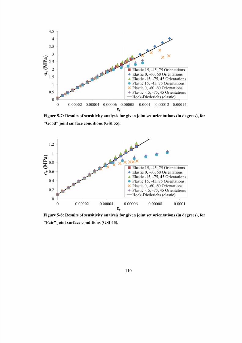
8/11/2019 Numerical Validation and Refinement of Empirical Rock Mass Modulus
http://slidepdf.com/reader/full/numerical-validation-and-refinement-of-empirical-rock-mass-modulus 130/263
Figure 5-7: Results of sensitivity analysis for given joint set orientations (in degrees), for
"Good" joint surface conditions (GSI 55).

8/11/2019 Numerical Validation and Refinement of Empirical Rock Mass Modulus
http://slidepdf.com/reader/full/numerical-validation-and-refinement-of-empirical-rock-mass-modulus 131/263
Figure 5-9: Results of sensitivity analysis for given joint set orientations (in degrees), for
"Poor" joint surface conditions (GSI 35).
5 3 Fi l A l i

8/11/2019 Numerical Validation and Refinement of Empirical Rock Mass Modulus
http://slidepdf.com/reader/full/numerical-validation-and-refinement-of-empirical-rock-mass-modulus 132/263
5.3 Final Analysis
The results of all the block models are summarized graphically in Figure 5-11 using both standard
and logarithmic scales for Erm to illustrate the difference between the empirical relationship and
the modelling results. The Erm data point for each elastic joint model has been back-calculated
from the slope of its associated numerical model stress and strain data. The data points for the
plastic joint models are labeled by the associated model runs from Figure 5-1. Models where the
joints behave plastically have a non-linear response, and therefore to estimate a back-calculated
value for Erm the slope of the secant to the stress vs. strain curve defined by the model data was
fitted to the point at which the non-linear portion becomes stable (when the rate of the increase in
strain doesn’t change with an increase in stress, Figure 5-12). The consequence of this approach
is that the Erm (plastic) will always be softer than Erm (elastic), because some amount of post-peak
behaviour of the joints is included in the Erm, and the models exhibit strain softening behaviour.
From Figure 5-11 it can be concluded that the models are stiffer than Hoek-Diederichs in the high
end of GSI, while softer in the low end of GSI.

8/11/2019 Numerical Validation and Refinement of Empirical Rock Mass Modulus
http://slidepdf.com/reader/full/numerical-validation-and-refinement-of-empirical-rock-mass-modulus 133/263
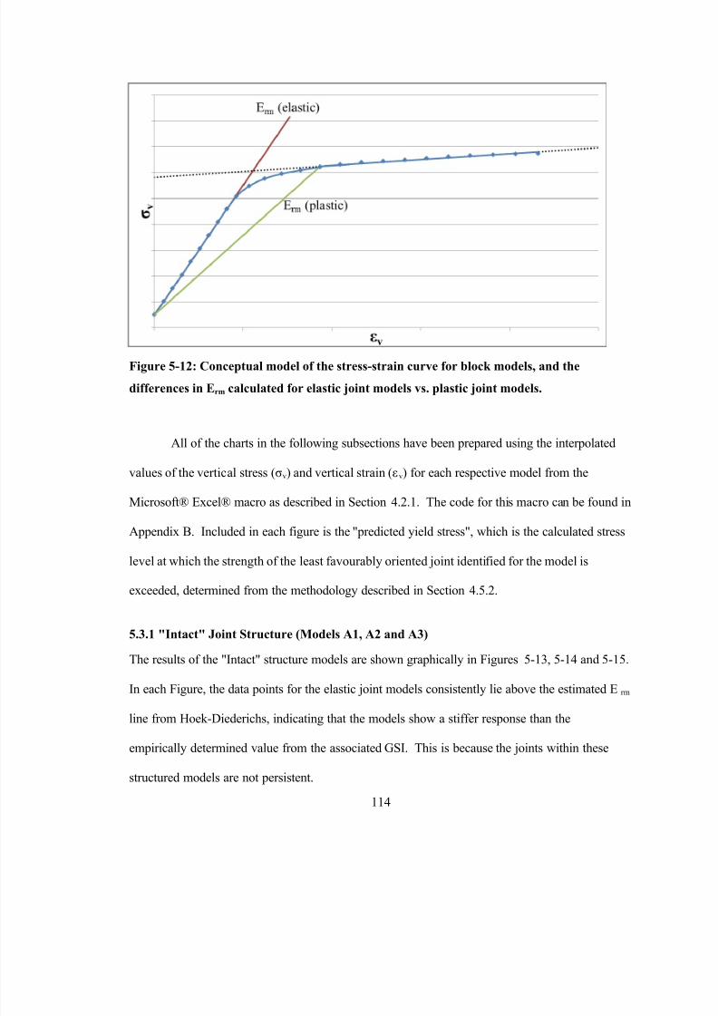
8/11/2019 Numerical Validation and Refinement of Empirical Rock Mass Modulus
http://slidepdf.com/reader/full/numerical-validation-and-refinement-of-empirical-rock-mass-modulus 134/263
The data points for the plastic joint models in each figure shows a divergence from the

8/11/2019 Numerical Validation and Refinement of Empirical Rock Mass Modulus
http://slidepdf.com/reader/full/numerical-validation-and-refinement-of-empirical-rock-mass-modulus 135/263
The data points for the plastic joint models in each figure shows a divergence from the
elastic joint models and becomes non-linear at the "Predicted Yield Stress" line, indicating that
the failure of the least favourable joint set with respect to the load, influences the deformational
response of the model.
Figure 5-13: Results of model A1 (GSI 90) using elastic and plastic joint properties.

8/11/2019 Numerical Validation and Refinement of Empirical Rock Mass Modulus
http://slidepdf.com/reader/full/numerical-validation-and-refinement-of-empirical-rock-mass-modulus 136/263
Figure 5-15: Results of model A3 (GSI 70) using elastic and plastic joint properties.
5.3.2
"Blocky" Joint Structure (Models B1, B2, B3, B4 and B5)
The results of the "Blocky" structured models are shown graphically in Figures 5-16 to 5-20.
Data points for the elastic joint models are very close to the line defined by the Hoek-Diederichs
empirical relationship for the associated GSI of the model. This was the desired effect because
the calibration was performed using the joint set structure of these models. The plastic joints in
all models have the same stiffness as the elastic joint models for stress levels below the

8/11/2019 Numerical Validation and Refinement of Empirical Rock Mass Modulus
http://slidepdf.com/reader/full/numerical-validation-and-refinement-of-empirical-rock-mass-modulus 137/263
Figure 5-16: Results of model B1 (GSI 75) using elastic and plastic joint properties.

8/11/2019 Numerical Validation and Refinement of Empirical Rock Mass Modulus
http://slidepdf.com/reader/full/numerical-validation-and-refinement-of-empirical-rock-mass-modulus 138/263
Figure 5-18: Results of model B3 (GSI 55) using elastic and plastic joint properties.

8/11/2019 Numerical Validation and Refinement of Empirical Rock Mass Modulus
http://slidepdf.com/reader/full/numerical-validation-and-refinement-of-empirical-rock-mass-modulus 139/263
Figure 5-20: Results of model B5 (GSI 35) using elastic and plastic joint properties.
5.3.3 "Very Blocky" Joint Structure (Models C1, C2, C3, C4 and C5)
The results of models with a GSI structure of "Very Blocky" are shown graphically in Figures
5-21 to 5-25. In the numerical models where the joints are not allowed to slip (behave
elastically), the data points lie on or above the empirically estimated Erm in the "Fair" to "Very
Good" quality surface conditions of models C3, C2 and C1. A noticeably softer response is seen
from the data points of both elastic and plastic joints in the models C4 and C5 representing the
poorest of joint surface conditions as compared to the empirical formula prediction. The point of

8/11/2019 Numerical Validation and Refinement of Empirical Rock Mass Modulus
http://slidepdf.com/reader/full/numerical-validation-and-refinement-of-empirical-rock-mass-modulus 140/263
Figure 5-21: Results of model C1 (GSI 65) using elastic and plastic joint properties.

8/11/2019 Numerical Validation and Refinement of Empirical Rock Mass Modulus
http://slidepdf.com/reader/full/numerical-validation-and-refinement-of-empirical-rock-mass-modulus 141/263
Figure 5-23: Results of model C3 (GSI 45) using elastic and plastic joint properties.

8/11/2019 Numerical Validation and Refinement of Empirical Rock Mass Modulus
http://slidepdf.com/reader/full/numerical-validation-and-refinement-of-empirical-rock-mass-modulus 142/263

8/11/2019 Numerical Validation and Refinement of Empirical Rock Mass Modulus
http://slidepdf.com/reader/full/numerical-validation-and-refinement-of-empirical-rock-mass-modulus 143/263
Figure 5-27: Results of model D2 (GSI 45) using elastic and plastic joint properties.

8/11/2019 Numerical Validation and Refinement of Empirical Rock Mass Modulus
http://slidepdf.com/reader/full/numerical-validation-and-refinement-of-empirical-rock-mass-modulus 144/263
Figure 5-29: Results of model D4 (GSI 25) using elastic and plastic joint properties.
Results of the block models show that the calibrated joint parameters in the jointed rock mass

8/11/2019 Numerical Validation and Refinement of Empirical Rock Mass Modulus
http://slidepdf.com/reader/full/numerical-validation-and-refinement-of-empirical-rock-mass-modulus 145/263
models produce an excellent correlation between the back-calculated values for E rm and the
empirically estimated value on the basis of a GSI quality ranging from 35-70 (Figure 5-11), when
the joints behave elastically. The models within this range include B2 to B5, C1 to C4 and D1 to
D3. The closest match out of all the varied structure of the block models are those of the
"Blocky" models. This was the desired result, as the Generalized Hoek-Diederichs empirical
equation was derived dominantly from in situ tests of similar quality of rock masses within this
range. It is generally observed that in poorer quality rock masses having a GSI < 35, the block
models show a softer response than the Erm predicted empirically, while in higher quality rock
masses (GSI > 70) the models show a stiffer response.
The Chinese and Taiwanese data set used in the original development of the Hoek-
Diederichs empirical relationship has limited data at both low- and high-end rock mass qualities.
Only 7% of the data was for higher quality rock masses (GSI 80 or higher), and only 13% of the
data was for lower quality rock masses (less than GSI 40). In this sense the mathematical
formula, derived from commercial curve fitting software (Hoek & Diederichs 2006) would
obviously favour the trend on the basis of the key 40-80 GSI range. This gives rise to a decreased
The "Intact" models A1, A2 and A3 are not fully persistent, as is the case in the other,

8/11/2019 Numerical Validation and Refinement of Empirical Rock Mass Modulus
http://slidepdf.com/reader/full/numerical-validation-and-refinement-of-empirical-rock-mass-modulus 146/263
denser joint models. The calibration of the joint stiffness properties, as described in Section
4.4.1.2, was performed assuming fully persistent joint sets. The simulated rock bridges between
the discontinuous joints increase the stiffness overall of the rock mass because the load is partly
carried across them.
The second reasoning theorized for the stiffer joint models may be related to the
problems associated with the in situ testing methods, as discussed by Hoek & Diederichs (2006).
Over 85% of the testing methods for the in situ Erm data used in the Generalized Hoek-Diederichs
formula involved Plate Tests (Hoek & Diederichs 2006). In situ methods, such as the PJT or PLT
methods, require the excavation to be present prior to performing the test. This excavation will
have an associated zone of influence, where the in situ rock is relaxed and potentially damaged as
a result of the excavation process. While it was assumed that the upper bound of the data set used
for the Generalized Hoek-Diederichs formula represented undisturbed, confined and undamaged
rock (Hoek & Diederichs 2006), for practical reasons it is not usually possible to install an
extensometer or measure deformation instantaneously following the excavation to avoid the
effects of relaxation near the excavation. The disturbance factor, D, has been created to account
results between the back-calculated value for Erm from numerical models and that estimated using

8/11/2019 Numerical Validation and Refinement of Empirical Rock Mass Modulus
http://slidepdf.com/reader/full/numerical-validation-and-refinement-of-empirical-rock-mass-modulus 147/263
the Generalized Hoek-Diederichs empirical equation, occurs in rock masses defined structurally
as "Blocky/Disturbed/Seamy" (models D3 to D5). Furthermore, the poorer the quality of the rock
mass, the greater this discrepancy becomes. The difference can be explained in terms of the
difficulty associated with determining Erm either in a lab setting or in situ in poor rock mass
quality.
In a lab setting, which is what the block models used in this analysis represent, the rock
mass is out of its natural in situ state even at the scale assumed in these models. As such the
sample no longer has the confinement of the rock mass acting on it. In the block model, no
confinement is applied laterally as the rock mass sample is compressed vertically. The additional
degree of freedom accommodates a greater localized strain in the rock mass, and consequently a
reduced modulus. In contrast, if the rock mass of an equivalent quality is confined as is the case
in an in situ test, this will reduce the amount of localized strain in the rock mass and therefore
increase the modulus. The effect is increased for poorer quality rock masses as the greater
amount of displacement can be accommodated due to the lack of confinement.
A second issue may be related to the rock mass characterization method used for the
A third factor contributing to the discrepancy between empirical and numerical results at

8/11/2019 Numerical Validation and Refinement of Empirical Rock Mass Modulus
http://slidepdf.com/reader/full/numerical-validation-and-refinement-of-empirical-rock-mass-modulus 148/263
poor rock mass quality is that the numerical models D1 to D5 are the densest models of all, and
with this increased model size the limitations of computer processing ability have been
encountered. The meshing of these models is of poorer quality relative to the less structurally
dense numerical models. Memory and computer processing limitations prevented the refinement
of the mesh by increasing the mesh resolution. The combination of this, along with the structure
defined by the relative orientations of joint sets in these models, resulted in a greater relative
number of elements with large aspect ratios with respect to the total number of elements as
compared to the "Intact/Massive", "Blocky" and "Very Blocky" structured models. This could
cause localized numerical instabilities during computation, therefore affecting the results. With
increased computer processing ability in the future it may be possible to refine the mesh further
so as to minimize the number of poor quality mesh elements.
5.5 References
Hoek, E., & Brown, E. (1997). Practical Estimates of Rock Mass Strength. Int J Rock Mech
Mining Sci, 34(8).
Hoek, E., & Diederichs, M. (2006). Empirical Estimation of Rock Mass Modulus. Int J Rock
Mech Mining Sci 43(2) 203-215
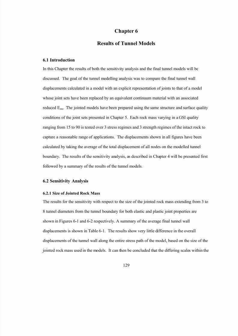
8/11/2019 Numerical Validation and Refinement of Empirical Rock Mass Modulus
http://slidepdf.com/reader/full/numerical-validation-and-refinement-of-empirical-rock-mass-modulus 149/263

8/11/2019 Numerical Validation and Refinement of Empirical Rock Mass Modulus
http://slidepdf.com/reader/full/numerical-validation-and-refinement-of-empirical-rock-mass-modulus 150/263
extending from the tunnel wall boundary, for joints with the Barton-Bandis shear strength

8/11/2019 Numerical Validation and Refinement of Empirical Rock Mass Modulus
http://slidepdf.com/reader/full/numerical-validation-and-refinement-of-empirical-rock-mass-modulus 151/263
criterion.
Table 6-1: Final tunnel wall displacements for models of varying sized jointed rock mass
Extent of
Jointed
Rock mass
(Diameters)
Total Final Average Displacement
(mm)
Elastic
Joints Plastic Joints
3 5.7 9.6
4 5.7 9.5
5 5.7 9.4
6 5.7 9.57 5.7 9.5
8 5.7 9.5
6.2.2
Width of Representative Boundary
The representative boundary separates the jointed rock mass from the external boundary of the
model, to avoid potential boundary effects arising from the joint networks intersecting the
external boundary. The results of sensitivity with respect to the width of this boundary, relative
to the size of the jointed rock mass, are shown in Figure 6-3. The boundary width has very little
effect on the displacements of the tunnel wall given by the model. At no internal pressure, a
maximum difference in the final average tunnel displacement of 6% occurs between the model
with no buffer zone and the model with a buffer zone 1/2 the width of the jointed rock mass. It is
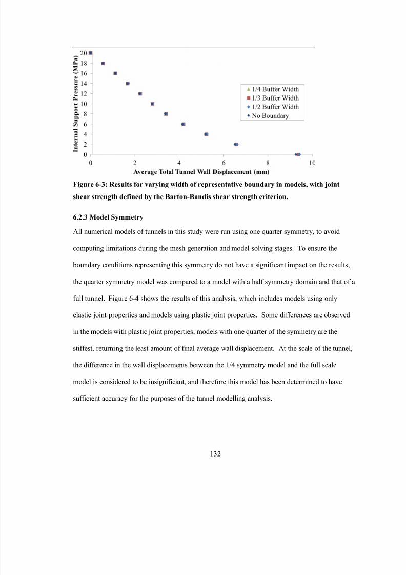
8/11/2019 Numerical Validation and Refinement of Empirical Rock Mass Modulus
http://slidepdf.com/reader/full/numerical-validation-and-refinement-of-empirical-rock-mass-modulus 152/263
Figure 6-3: Results for varying width of representative boundary in models, with joint
shear strength defined by the Barton-Bandis shear strength criterion.
6.2.3 Model Symmetry
All numerical models of tunnels in this study were run using one quarter symmetry, to avoid
computing limitations during the mesh generation and model solving stages. To ensure the
boundary conditions representing this symmetry do not have a significant impact on the results,
the quarter symmetry model was compared to a model with a half symmetry domain and that of a
full tunnel. Figure 6-4 shows the results of this analysis, which includes models using only

8/11/2019 Numerical Validation and Refinement of Empirical Rock Mass Modulus
http://slidepdf.com/reader/full/numerical-validation-and-refinement-of-empirical-rock-mass-modulus 153/263
Figure 6-4: Results of sensitivity of model symmetry for models with elastic joint properties
and plastic joint properties.
6.3
Tunnel Modelling Results
Results for all tunnel models, for both the jointed rock mass and equivalent continuum models are
presented in this section. The computed displacements for each model type included in the
analysis are compared over all combinations of stress and strength of the intact rock. This matrix
along with the associated abbreviated terms is given in Table 6-2.
Table 6-2: Matrix of tunnel model runs and associated abbreviated terms for the different
Torres (2004) (the C-T solution) is built directly in to the program Rocsupport (Rocscience Inc.

8/11/2019 Numerical Validation and Refinement of Empirical Rock Mass Modulus
http://slidepdf.com/reader/full/numerical-validation-and-refinement-of-empirical-rock-mass-modulus 154/263
2010) and was used for this analysis. To meaningfully compare elastic-only properties in Figure
6-5, the strength properties used in the C-T solution were set intentionally high to prevent any
failure of the rock material, so that all displacements predicted using this analytical solution are
only associated with Erm. In the figures of the proceeding subsections, this is referred to as C-T
(elastic). It will also be shown in the following subsections that the results predicted analytically
from the C-T solution are very similar to the equivalent elastic and plastic continuum FEM
models. In both Figures 6-5 and 6-6, the "% Difference" used for the vertical axis is determined
from the following equation:
ifference (d jdT)
averaged j, dT
(6-1)
where d j is the final average tunnel wall displacement predicted in the jointed rock mass model,
and d-T is the final wall displacement predicted using the C-T solution.
The results summarized in Figure 6-5 show that the majority of the displacements
predicted by a numerical model of a jointed rock mass are less than those predicted in an
equivalent analytical model using the C-T (elastic) solution. The only models with displacements

8/11/2019 Numerical Validation and Refinement of Empirical Rock Mass Modulus
http://slidepdf.com/reader/full/numerical-validation-and-refinement-of-empirical-rock-mass-modulus 155/263
Figure 6-5: Summary of final tunnel wall displacements predicted in models with elastic
joint and elastic intact rock models compared to displacements predicted from the
Carranza-Torres (2004) analytical solution with elastic-only displacements.
The rock mass strength properties used for the C-T solution presented in Figure 6-6 were
estimated using Eqs. (2-13), (2-14) and (2-15) (page 40) from the representative GSI and the
strength of the intact rock of the associated jointed rock mass model. In the figures of the

8/11/2019 Numerical Validation and Refinement of Empirical Rock Mass Modulus
http://slidepdf.com/reader/full/numerical-validation-and-refinement-of-empirical-rock-mass-modulus 156/263
Figure 6-6: Summary of final tunnel wall displacements predicted in models with plastic joint and plastic intact rock properties compared to displacements predicted from the fully
plastic Carranza-Torres (2004) analytical solution
6.3.1
Results of Models for S1D1
The results of all models run using the highest relative stress level and highest relative strength of
the intact rock are shown in Figure 6-7. In higher quality rock masses (higher than GSI 55),

8/11/2019 Numerical Validation and Refinement of Empirical Rock Mass Modulus
http://slidepdf.com/reader/full/numerical-validation-and-refinement-of-empirical-rock-mass-modulus 157/263
Figure 6-7: Results for models of high intact rock strength in a 35 MPa hydrostatic stress
field (S1D1).
Table 6-3: Varied tunnel wall displacements calculated in models with plastic joints and
perfectly-plastic intact rock depending on the structure of jointed rock mass
GSI Assigned
to Rock mass
Joint Structure in Model and
Total Final Average Displacement (mm)
Blocky Very Blocky Blocky/Disturbed/Seamy
35 17 228 104
45 9 26 24
6.3.2
Results of Models for S1D2

8/11/2019 Numerical Validation and Refinement of Empirical Rock Mass Modulus
http://slidepdf.com/reader/full/numerical-validation-and-refinement-of-empirical-rock-mass-modulus 158/263
Figure 6-8: Results for models of high intact rock strength in a 20 MPa hydrostatic stress
field (S1D2).
6.3.3
Results of Models for S1D3
The results of all models run using the lowest relative stress level and a high strength of intact
rock are given in Figure 6-9. As was the case with the previous two subsections discussing high
strength for intact rock, a large amount of displacement occurs when joints that behave plastically
are used in the model of poorer quality rock masses. The continuum-based models (including the
C-T results) predict similar displacements whether the rock behaves plastically or not, across the

8/11/2019 Numerical Validation and Refinement of Empirical Rock Mass Modulus
http://slidepdf.com/reader/full/numerical-validation-and-refinement-of-empirical-rock-mass-modulus 159/263
Figure 6-9: Results for models of high intact rock strength in a 5 MPa hydrostatic stress
field (S1D3).
6.3.4
Results of Models for S2D1
The results of all models run at the highest stress level with medium strength for intact rock are
displayed in Figure 6-10. It is seen from this figure that in high quality rock masses the
displacements are larger when determined from both elastic and plastic continuum models. In
poorer quality rock masses the jointed models with plastic joints show similar displacement to
equivalent continuum models. Elastically, jointed models show less displacement than their

8/11/2019 Numerical Validation and Refinement of Empirical Rock Mass Modulus
http://slidepdf.com/reader/full/numerical-validation-and-refinement-of-empirical-rock-mass-modulus 160/263
Figure 6-10: Results for models of medium intact rock strength in a 35 MPa hydrostatic
stress field (S2D1).
6.3.5
Results of Models for S2D2
The results of all models run at a moderate stress level and a medium strength of intact rock are
given in Figure 6-11. The greatest displacements occur in the poorest of rock masses when
represented with plastic joints. All non-jointed plastic continuum and plastic jointed models are
also in close agreement of one another over the lower quality GSI range (GSI 35 and lower). In
this stress and strength regime, the elastic joint models show the least amount of displacements

8/11/2019 Numerical Validation and Refinement of Empirical Rock Mass Modulus
http://slidepdf.com/reader/full/numerical-validation-and-refinement-of-empirical-rock-mass-modulus 161/263

8/11/2019 Numerical Validation and Refinement of Empirical Rock Mass Modulus
http://slidepdf.com/reader/full/numerical-validation-and-refinement-of-empirical-rock-mass-modulus 162/263
Figure 6-12: Results for models of medium intact rock strength in a 5 MPa hydrostatic
stress field (S2D3).
6.3.7
Results of Models for S3D1
Illustrated in Figure 6-13 are the results for all models run at the highest stress level and the
lowest strength of intact rock. In contrast to models shown previously, all continuum-based
elastic and plastic models consistently predict more displacement when compared to their
respective elastic and plastic jointed model. Furthermore, equivalent plastic continuum numerical
models with perfectly plastic material predict complete tunnel collapse (displacement equal to the

8/11/2019 Numerical Validation and Refinement of Empirical Rock Mass Modulus
http://slidepdf.com/reader/full/numerical-validation-and-refinement-of-empirical-rock-mass-modulus 163/263
Figure 6-13: Results for models of low intact rock strength in a 35 MPa hydrostatic stress
field (S3D1).
6.3.8 Results of Models for S3D2
Figure 6-14 shows the results of all models run at a medium relative stress level and the lowest
strength for the intact rock. There is a very little difference in predicted displacements in models
with elastic joints and elastic intact rock over the GSI range. This type of model is considered to
have the stiffest response within this strength and stress regime. In the poorest quality rock

8/11/2019 Numerical Validation and Refinement of Empirical Rock Mass Modulus
http://slidepdf.com/reader/full/numerical-validation-and-refinement-of-empirical-rock-mass-modulus 164/263
Figure 6-14: Results for models of low intact rock strength in a 20 MPa hydrostatic stress
field (S3D2).
6.3.9
Results of Models for S3D3
Results shown in Figure 6-15 are models that were run at the lowest stress level and the lowest
relative strength of intact rock. Representative models with no joints and plastic material
properties show larger displacements than their respective equivalent jointed rock mass models,
over the entire GSI range. In all models with plastic joints having a GSI quality of 35 or less, it

8/11/2019 Numerical Validation and Refinement of Empirical Rock Mass Modulus
http://slidepdf.com/reader/full/numerical-validation-and-refinement-of-empirical-rock-mass-modulus 165/263
Figure 6-15: Results for models of low intact rock strength in a 5 MPa hydrostatic stress
field (S3D3).
6.4 Discussion of Results
The results of this analysis show certain differences and similarities to predicted tunnel wall
displacements when the rock mass surrounding the tunnel is modelled using an explicit
representation of joints versus a representative continuum medium without joints. The
similarities occur in higher quality rock masses with high intact rock strength, and the differences
are found when both the quality of the rock mass and the intact rock strength are reduced. None
mass only deforms elastically, as confirmed by the results of the elastic models showing very

8/11/2019 Numerical Validation and Refinement of Empirical Rock Mass Modulus
http://slidepdf.com/reader/full/numerical-validation-and-refinement-of-empirical-rock-mass-modulus 166/263
similar results within this range.
As the strength of the intact rock is reduced, the displacements predicted in the
continuum-based models are greater than those shown in the models with a jointed rock mass at
this higher end of GSI. In this situation the jointed rock mass models do not necessarily deform
uniformly away from the tunnel excavation. When a tunnel is excavated the stress state is
redistributed to achieve a new state of equilibrium. In a numerical representation of a jointed
rock mass, this equilibration is achieved by the deformation of the joint elements preferentially,
as they are softer than the intact rock between them. It is theorized that the stress redistribution,
in the form of displacements, occurs in a smaller zone surrounding the tunnel for the jointed
models than does the continuum based models. As the quality of the rock mass is high, any
failure of the joints (slip) in models where joint strength is defined is localized, and is not the
cause of significant displacement. In reality, this is due to confinement acting on the joints in the
rock mass, which increases with distance away from the excavation.
Another explanation analogous to the aforementioned reasoning has already been
described in Chapter 5. To reiterate, the original formulation of the Generalized Hoek-Diederichs
Across all strength and stress regimes within the medium quality of rock masses (35-45 GSI), the

8/11/2019 Numerical Validation and Refinement of Empirical Rock Mass Modulus
http://slidepdf.com/reader/full/numerical-validation-and-refinement-of-empirical-rock-mass-modulus 167/263
jointed rock mass models show the greatest variance in calculated displacements, in some
instances by an order of magnitude for the same quality (i.e. GSI assigned value) of rock mass as
shown in Table 6-3. It is within this quality of rock mass where the strength of the joints begin to
govern the displacements in the models, as is evident from the fact that they differ significantly
from models where the joints behave elastically. Within the GSI rock mass classification system,
it is possible to have two rock masses with different structure and surface conditions for the
discontinuities, to have the same GSI rating. The models in this research show the amount of
displacement differs depending on the structure and surface conditions of the joints, regardless
whether they are of equivalent quality in terms of the GSI classification system. The theorized
explanation is because the larger displacements seen in the "Very Blocky" are a result of a
combination between the strength of the joints in the model, their density and orientation relative
to one another. The situation leads to an "optimal" condition for reduced block interlocking, and
while this model contains fewer joint sets than the "Blocky/Disturbed/Seamy" model, the degree
of interlocking may be insufficient to overcome the failure as a result of the weaker surface
conditions, leading to greater failure of the joint elements and larger displacements. The
In the poorest of quality rock masses, it can be concluded that rock mass strength is the dominant

8/11/2019 Numerical Validation and Refinement of Empirical Rock Mass Modulus
http://slidepdf.com/reader/full/numerical-validation-and-refinement-of-empirical-rock-mass-modulus 168/263
factor in the calculation of the displacements. The strength of the rock mass in the equivalent
plastic continuum models is estimated on the basis of the strength of intact rock of the jointed
rock mass model and its associated GSI. When the jointed rock mass models have high intact
rock strength, the associated estimated strength for equivalent plastic continuum models is such
that no significant failure occurs, resulting in less predicted displacements than the jointed rock
mass models.
Conversely, when the strength of intact rock in the jointed rock mass models is low, the
equivalent plastic continuum models show considerable failure and displacements due to the very
low estimated strength parameters. In this case, the jointed rock mass models are very similar to
the equivalent elastic continuum model results, rather than equivalent plastic continuum results.
A possible explanation for the significant differences in the displacements between plastic jointed
rock mass models and equivalent plastic continuum models is due to the unreliability associated
with estimating GSI using adjusted RMR values as discussed in Chapter 5. These results
therefore would appear to confirm the statement made by Marinos et al. (2005) that the
correlation of an adjusted RMR value with GSI, when used to provide input for the GHB
joints are very tight from the confinement and therefore have a response more similar to that of

8/11/2019 Numerical Validation and Refinement of Empirical Rock Mass Modulus
http://slidepdf.com/reader/full/numerical-validation-and-refinement-of-empirical-rock-mass-modulus 169/263
the intact rock between them. A confirmation of this reasoning pertaining to the strength is
shown in Figure 6-16, where the extent of the yielded zone in the jointed rock mass models is
found to be smaller than the equivalent continuum models.
Figure 6-16: Comparison of yielding between a jointed rock mass model of "Very Blocky"
structure and "Very Poor" discontinuity surface conditions and the equivalent continuum
model (Left) Extent of yielded joint elements in a jointed rock mass model with plastic
of a rock mass to the strength of an equivalent continuum rock mass is necessary in order to
di l i hi H l i b d hi h i d b l i

8/11/2019 Numerical Validation and Refinement of Empirical Rock Mass Modulus
http://slidepdf.com/reader/full/numerical-validation-and-refinement-of-empirical-rock-mass-modulus 170/263
discern a relationship. However, a correlation can be made which is presented subsequently in
Section 7.2.2 between the numerical representation of a fully elastic jointed rock mass and an
equivalent elastic continuum. It is therefore the view of this author that the deformation property
of Erm, when estimated empirically using the Hoek-Diederichs method for the purpose of the
FEM modelling of a tunnel, should not include the deformation contribution of slip along the
joints.
6.6 References
Marinos, V., Marinos, P., & Hoek, E. (2005). The Geological Strength Index: Applications and
Limitations. Bull Eng. Geol. Environ., 64, 55-65.
Chapter 7

8/11/2019 Numerical Validation and Refinement of Empirical Rock Mass Modulus
http://slidepdf.com/reader/full/numerical-validation-and-refinement-of-empirical-rock-mass-modulus 171/263
Discussions and Conclusions
This research has been focused on understanding the role of numerical modelling programs for
tunnel excavation analysis, and the representative input parameters that go into them. Specific to
FEM numerical analyses, input parameters that are used to define rock mass strength and
deformation can be estimated using empirical relationships with rock mass classification systems.
This research has concentrated on deformation parameter estimation using the empirical
relationship of Hoek & Diederichs (2006) between Erm and GSI.
7.1 Summary of Findings
A methodology has been proposed demonstrating that it is possible to calibrate the main
properties of discontinuities for a numerical model, in the form of UCS test block models as a
method to model the overall deformation in a rock mass consisting of an isotropic network of
joint systems. An approach has been proposed for the numerical generation of a rock mass based
on the structure and density of the major joint sets, as well as their surface conditions as
characterized by GSI.
variance in the predicted unsupported tunnel wall displacements. It was found that the degree of
i i t d i lit k (GSI 35 l ) h th j i t i th

8/11/2019 Numerical Validation and Refinement of Empirical Rock Mass Modulus
http://slidepdf.com/reader/full/numerical-validation-and-refinement-of-empirical-rock-mass-modulus 172/263
variance is most pronounced in poorer quality rock masses (GSI 35 or less) when the joints in the
jointed models behave plastically. When both the jointed models and the equivalent continuum
models are defined using elastic properties, the resulting displacements are greater in all
continuum models than the jointed models, suggesting the empirical relationship underestimates
Erm within this range. A modification to the empirical Hoek-Diederichs for tunnels is proposed to
deal with this underestimation specific to tunnelling applications.
7.2 Discussion
This research has been aimed at investigating rock mass deformation behaviour for tunnels using
FEM numerical analysis. The analysis performed assumes that overall behaviour of the rock
mass is dominantly controlled by the associated stiffness and strength parameters of the
discontinuities. For a FEM numerical model, the representative overall behaviour is described in
terms of an elastic component (i.e. the stiffness) and a strength component (i.e. the failure
envelope and post-yield parameters).
7.2.1
Representative Behaviour of Erm in FEM Analysis
Th d fi i i f E i l d b h l i d i l i b h i H i FEM
slip behaviour of the joints and other inelastic joint movement (i.e. dilation) should be handled by
th t ti t th it i d l ti fl l

8/11/2019 Numerical Validation and Refinement of Empirical Rock Mass Modulus
http://slidepdf.com/reader/full/numerical-validation-and-refinement-of-empirical-rock-mass-modulus 173/263
the representative strength criteria and plastic flow rules.
Chapter 5 presented the investigation of joint behaviour under loading conditions, and
whether the associated rock mass quality defined by their structure and surface conditions can be
accurately modeled with representative stiffness properties estimated empirically for a continuum
model. When slip is allowed to occur along joints within the FEM numerical models, the jointed
models show a softer response than the predicted Erm from the rock mass quality in terms of its
GSI. The non-linearity of the deformation when slip is allowed along the joints occurs at the
point where the strength of the least favourable joint is exceeded. This can be viewed as the yield
point of the jointed rock mass.
Chapter 6 investigated the unloading conditions of a tunnel excavation to see whether the
assumption that the representative Erm estimated from the Generalized Hoek-Diederichs formula
is valid. A large scatter is present in the displacement results between a jointed rock mass and an
equivalent continuum model when a plasticity model is used for the joint behaviour and in the
equivalent continuum model. It is suggested that this is an artifact of not having calibrated the
strength used for the joints with a representative strength of an equivalent rock mass.
relative movements of the intact rock between them. The in situ test for the determination of Erm
involves the creation of the excavated adit (an initial unloading of the rock mass) followed by the

8/11/2019 Numerical Validation and Refinement of Empirical Rock Mass Modulus
http://slidepdf.com/reader/full/numerical-validation-and-refinement-of-empirical-rock-mass-modulus 174/263
involves the creation of the excavated adit (an initial unloading of the rock mass), followed by the
application of the test to the rock mass (a subsequent loading to the rock mass). For a tunnel, the
goal is to estimate the rock mass behaviour during the initial unloading event, in order to
determine the support or reinforcement required. It is the results of this subsequent loading
during the PLT or PJT that are being used to describe the representative deformational behaviour
of the rock mass. However, the initial unloading of the rock mass changes it from its natural in
situ state and the test results are affected by this change. An example of the alteration includes
the re-alignment of the asperities of the discontinuities due to relative movements of the intact
rock during unloading.
Results from the tunnelling analysis have shown an underestimation of E rm as a
representative parameter for the elastic jointed rock mass numerical model, for rock masses
having a GSI characterization of 35 or less. Within this quality of rock mass, it has been shown
numerically that the extent of underestimation has an inverse relationship with the Young’s
modulus (Ei). Two complementary rationales are hypothesized in this regard.
The first explanation is related to issues associated with the lab determination of E i in soft
linear initially ('A' portion of curve (ii) in Figure 7-1), where the sample is undergoing closure of
this internal microstructure The extent of this closure is greater than in the case of the same rock

8/11/2019 Numerical Validation and Refinement of Empirical Rock Mass Modulus
http://slidepdf.com/reader/full/numerical-validation-and-refinement-of-empirical-rock-mass-modulus 175/263
this internal microstructure. The extent of this closure is greater than in the case of the same rock
sample found in situ, due to the confinement provided by the in situ stresses. The consequence,
with respect to the interpretation of the lab testing, is that a greater error will be associated with
respect to the differences in the internal microstructure of different samples in soft rock. In
harder rock this is less of a problem because there is a smaller percentage of microstructure
present in the sample, and because of its competency, it is less likely to be disturbed during the
recovery and preparation process. This is known as sampling error, and can result in the lab test
results for Ei to be less than the actual value of the rock in situ. Consequently, if the actual value
of Ei is greater than the lab result, so too must be the value for Erm, since these parameters are
directly proportional to one another in the Generalized Hoek-Diederichs empirical formula.

8/11/2019 Numerical Validation and Refinement of Empirical Rock Mass Modulus
http://slidepdf.com/reader/full/numerical-validation-and-refinement-of-empirical-rock-mass-modulus 176/263
The scaling factor as a function of Ei increases the estimated value for Erm over the
original formula both with a decrease in Ei as well as a decrease in GSI As both the GSI and the

8/11/2019 Numerical Validation and Refinement of Empirical Rock Mass Modulus
http://slidepdf.com/reader/full/numerical-validation-and-refinement-of-empirical-rock-mass-modulus 177/263
original formula both with a decrease in Ei as well as a decrease in GSI. As both the GSI and the
Ei are increased to more competent rock masses and harder intact rock respectively, Ce will trend
towards 1. This is a reflection on the results of this analysis, where the differences between the
displacements in the jointed models from those in the equivalent continuum models are gradually
reduced both as a function of increased competency of the rock mass and the Ei of the material.
This represents a conservative modification on the basis of the results found in this analysis. The
relative effect of Eq. (7-1) over Eq. (2-17) to the estimated Erm is plotted in log(Erm)-GSI space
for Ei values of 1, 2, 5, 10, 20, 50 and 100 GPa respectively in Figure 7-2.
Fi 7 2 P d G li d H k Di d i h difi ti f T l (L ft) E
The simple change results in decreased amount of correction in rock with low E i and in
low quality rock masses When plotted as a ratio to the estimated value for E predicted from

8/11/2019 Numerical Validation and Refinement of Empirical Rock Mass Modulus
http://slidepdf.com/reader/full/numerical-validation-and-refinement-of-empirical-rock-mass-modulus 178/263
low quality rock masses. When plotted as a ratio to the estimated value for Erm predicted from
the original Generalized Hoek-Diederichs equation against GSI (Figure 7-3), the differences over
a number of Ei become immediately apparent.
Figure 7-3: Ratio of Erm predicted from correction equation (7-1) to the Generalized Hoek-
Diederichs estimation vs. GSI, with modifications of the exponent in Eq. (7-2) (Left) Using a
value of 0.5 (Right) Using a value of 0.6
The second adjustment proposed in in Eq. (7-4) also considers a correction factor Ce,
however in Eq. (7-5) it is expressed as both a function of Ei and GSI.
included to reflect the greater displacements in the jointed rock mass model over the equivalent
continuum model when Ei was greatest and GSI was less than 35 The relative effect of Eq (7-4)

8/11/2019 Numerical Validation and Refinement of Empirical Rock Mass Modulus
http://slidepdf.com/reader/full/numerical-validation-and-refinement-of-empirical-rock-mass-modulus 179/263
continuum model, when Ei was greatest and GSI was less than 35. The relative effect of Eq. (7 4)
over Eq. (2-17) to the estimated Erm is plotted in log(Erm)-GSI space for Ei values of 1, 2, 5, 10,
20, 50 and 100 GPa respectively in Figure 7-4.
Figure 7-4: Proposed Generalized Hoek-Diederichs modification for Tunnels (Left) Erm vs
GSI plot using a correction factor of Eq. (7-5) with D = 0 (Right) Erm vs GSI plot for
Generalized Hoek-Diederichs equation with D = 0.
It is noted that the original development of the Hoek-Diederichs empirical formula in Eq.
(2-17) was calibrated for loading (Diederichs, 2011), and it must be emphasized that the Eqs.
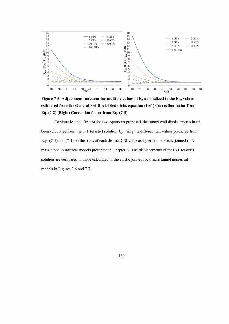
8/11/2019 Numerical Validation and Refinement of Empirical Rock Mass Modulus
http://slidepdf.com/reader/full/numerical-validation-and-refinement-of-empirical-rock-mass-modulus 180/263
Figure 7-5: Adjustment functions for multiple values of Ei, normalized to the Erm values
estimated from the Generalized Hoek-Diederichs equation (Left) Correction factor from
Eq. (7-2) (Right) Correction factor from Eq. (7-5).
To visualize the effect of the two equations proposed, the tunnel wall displacements have
been calculated from the C-T (elastic) solution, by using the different Erm values predicted from
Eqs. (7-1) and (7-4) on the basis of each distinct GSI value assigned to the elastic jointed rock
mass tunnel numerical models presented in Chapter 6. The displacements of the C-T (elastic)
solution are compared to those calculated in the elastic jointed rock mass tunnel numerical
models in Figures 7-6 and 7-7.

8/11/2019 Numerical Validation and Refinement of Empirical Rock Mass Modulus
http://slidepdf.com/reader/full/numerical-validation-and-refinement-of-empirical-rock-mass-modulus 181/263
Figure 7-6: Final tunnel wall displacements predicted in models with elastic joint and elastic
intact rock models compared to displacements predicted from the C-T (elastic) solution
(Left) From Erm estimated using Eq. (7-1) (Right) From Erm estimated using original
Generalized Hoek-Diederichs equation reproduced from Figure 6-5.
7.3 Recommendations for Future Work
The equivalent continuum tunnel models prepared in this research have assumed that the

8/11/2019 Numerical Validation and Refinement of Empirical Rock Mass Modulus
http://slidepdf.com/reader/full/numerical-validation-and-refinement-of-empirical-rock-mass-modulus 182/263
q p p
parameters for rock mass strength, as defined by the Generalized Hoek-Brown failure criterion,
are correctly estimated on the basis of the relevant GSI value assigned to the respective jointed
rock mass models. As the focus of this research was equating the cumulative deformation of the
joint networks within the jointed rock mass models to Erm, no work was done to explore how the
plastic deformation along the joints relate to the post-peak plastic flow of the rock mass strength.
Future work should explore this concept to obtain a more accurate representative model of the
full extent of joint behaviour. With reference to the poorer quality rock mass tunnel models, this
would involve determining the zonal extent of the rock mass for which strength in the equivalent
plastic continuum rock mass applies, from the extent of yielding found in the jointed rock mass
models.
The joint normal and joint shear stiffness parameters assigned to the jointed rock mass in
both the block and tunnel have been calibrated using a specific Ei, and do not vary in the tunnel
models with respect to the different strength regimes of the intact rock. The modifications to the
Generalized Hoek-Diederichs empirical formula are purposely conservative in this regard, as in
The effect of persistence of the discontinuities in the numerical models with respect to
this research has been described in Section 5.3.1. It should also be mentioned that the degree of

8/11/2019 Numerical Validation and Refinement of Empirical Rock Mass Modulus
http://slidepdf.com/reader/full/numerical-validation-and-refinement-of-empirical-rock-mass-modulus 183/263
g
persistence controls the degree of interlock of the rock blocks between the discontinuities, and an
incorporation of persistence in to the calibration of the joint parameters would be a logical choice
for future work.
7.4 Conclusion
Numerical modelling is an important tool for the engineering design of underground excavations.
Given the fact that most current numerical modelling software packages provide very robust
functionality, it is important that the user understand the functionality that is best suited to their
problem of interest, as well as the input data that goes into them. Limitations on the complexity
of the models and computer processing power require that representative behaviour from
representative input parameters be assumed within the numerical analysis. The FEM analysis
presented in this research emphasizes these important concepts, by including discussions on the
theory of elasticity and plasticity in a FEM numerical modelling context.
7.5
References

8/11/2019 Numerical Validation and Refinement of Empirical Rock Mass Modulus
http://slidepdf.com/reader/full/numerical-validation-and-refinement-of-empirical-rock-mass-modulus 184/263

8/11/2019 Numerical Validation and Refinement of Empirical Rock Mass Modulus
http://slidepdf.com/reader/full/numerical-validation-and-refinement-of-empirical-rock-mass-modulus 185/263
A.3 Comparisons of Tunnel Model Values Interpolated using the Macro Versus
Values Extracted from Phase2 Interpret

8/11/2019 Numerical Validation and Refinement of Empirical Rock Mass Modulus
http://slidepdf.com/reader/full/numerical-validation-and-refinement-of-empirical-rock-mass-modulus 186/263
Figure A-3: Support pressure versus Total Tunnel Wall Displacements for S1D3 elastic
jointed tunnel models of "Very Blocky" and "Very Poor" quality (GSI 25), comparing
values obtained from the macro and using Phase2 Interpret.

8/11/2019 Numerical Validation and Refinement of Empirical Rock Mass Modulus
http://slidepdf.com/reader/full/numerical-validation-and-refinement-of-empirical-rock-mass-modulus 187/263
Figure A-4: Support pressure versus Total Tunnel Wall Displacements for S1D3 tunnel
models with plastic joints and plastic intact rock of "Very Blocky" and "Very Poor" quality
(GSI 25), comparing values obtained from the macro and using Phase2 Interpret.

8/11/2019 Numerical Validation and Refinement of Empirical Rock Mass Modulus
http://slidepdf.com/reader/full/numerical-validation-and-refinement-of-empirical-rock-mass-modulus 188/263
Figure A-6: Support pressure versus Total Tunnel Wall Displacements for S3D1 tunnel
models with plastic joints and plastic intact rock of "Very Blocky" and "Very Poor" quality
(GSI 25), comparing values obtained from the macro and using Phase2 Interpret.
Table A-2: Comparison of data processing times for obtaining total displacement data from
one tunnel model computed Phase2 numerical models of "Very Blocky" structure.
Data Processing Method Total Data Processing Time (average
in minutes)

8/11/2019 Numerical Validation and Refinement of Empirical Rock Mass Modulus
http://slidepdf.com/reader/full/numerical-validation-and-refinement-of-empirical-rock-mass-modulus 189/263
Dim allText As StringDim lFD As FileDialogDim fileFilter As FileDialogFilters
Dim oApp As Object
Dim isFEZFile As BooleanDim fileItem As VariantDim folderName As Variant
Dim curText As String, stextBackup As String

8/11/2019 Numerical Validation and Refinement of Empirical Rock Mass Modulus
http://slidepdf.com/reader/full/numerical-validation-and-refinement-of-empirical-rock-mass-modulus 190/263
170
g, p g
''''''''''!!!!!!!!!!!!DATA STRUCTURES USED!!!!!!!!!!!!!'''''''''''''''''''''------------------------------------------------------------------------
'theQueryPoints[q][7] - For storing information regarding q query points |'----------------------|-------------------------------------------------'theQueryPoints[i][0] | The Element the i-th point is contained in |
'----------------------|------------------------------------------------|'theQueryPoints[i][1] | The X coordinate of the i-th point |'----------------------|------------------------------------------------|
'theQueryPoints[i][2] | The Y coordinate of the i-th point |
'----------------------|------------------------------------------------|'theQueryPoints[i][3] | The node number if the point falls on a node, |' | 0 otherwise |
'----------------------|------------------------------------------------|'theQueryPoints[i][j] | j=4,5,6 corresponding to the nodes of the sub |' | triangle the point is contained in |
'----------------------|------------------------------------------------|'------------------------------------------------------------------------
'allNodes[n][3] - For storing information regarding all the nodes |'----------------------|-------------------------------------------------'allNodes[i][0] | The node number |
'----------------------|------------------------------------------------|'allNodes[i][1] | The x-coordinate of the node |'----------------------|------------------------------------------------|
'allNodes[i][2] | The y-coordinate of the node |'----------------------|------------------------------------------------|'------------------------------------------------------------------------
'allElements[n][8] - For storing information regarding all the elements |'----------------------|-------------------------------------------------
'allElements[i][j] | j=1,2,3,4,5,6 corresponding the node numbers of|' | the element |'----------------------|------------------------------------------------|
'allElements[i][7] |0 - a material element; 1 - a joint element |
'----------------------|------------------------------------------------|'------------------------------------------------------------------------
'nodeElementList[qn][40] - For each node n associated with determining |
' q query points (qn nodes), each element the |
' node is common to. |'----------------------|------------------------------------------------|'nodeElementList[ni][0]|the node number |
'----------------------|------------------------------------------------|
'nodeElementList[ni][j]|j = 1 to 39, the element list the node is common|' |to. |'----------------------|------------------------------------------------|
'queryNodes[qn][40] - nodes associated with the query (subset of allnodes) |
8/11/2019 Numerical Validation and Refinement of Empirical Rock Mass Modulus
http://slidepdf.com/reader/full/numerical-validation-and-refinement-of-empirical-rock-mass-modulus 191/263
171
'----------------------|------------------------------------------------|'queryNodes[ni][0] |the re-coded node number for fast processing |
'----------------------|------------------------------------------------|'queryNodes[ni][1] |the node number as per the file |
'----------------------|------------------------------------------------|'queryNodes[ni][2] |the x-coordinate of the node |'----------------------|------------------------------------------------|
'queryNodes[ni][3] |the y-coordinate of the node |'----------------------|------------------------------------------------|
'queryElements[qe][8] - elements associated with the query (subset of |
' allelements) |
'----------------------|------------------------------------------------|'queryElements[ei][0] |the re-coded element number for fast processing |'----------------------|------------------------------------------------|
'queryElements[ei][1] |the element number as per the file |'----------------------|------------------------------------------------|'queryElements[ei][j] |j = 2 to 7, the node number as coded in |
' | queryNodes[ni][0] for faster processing |'----------------------|------------------------------------------------|
'queryElements[ei][3] |the y-coordinate of the node |'----------------------|------------------------------------------------|
'nodeXDisplacements[qn][sn] - The x-direction displacement value for each |
' node associated with the query (qn nodes), at |' each stage for sn stages. |
'nodeYDisplacements[qn][sn] - The y-direction displacement value for each |
' node associated with the query (qn nodes), at |' each stage for sn stages. |
'nodeXStresses[qn][sn] - The averaged, x-direction stress at each node |
' associated with the query (qn nodes), averaged from|' the values of the given nodal value associated with|
' each of its shared elements. |'nodeYStresses[qn][sn] - As above, for the y-direction stress |'nodeXYStresses[qn][sn]- As above, for the shear stress |
' EACH OF THE 5 HAVE THE FOLLOWING STRUCTURE (defined as ds) |
'----------------------|------------------------------------------------|'ds[ni][0] |the node number as coded in queryNodes[ni][0] |'----------------------|------------------------------------------------|
'ds[ni][j] |j = 1 to sn - the value for the given j-th stage|
'----------------------|------------------------------------------------|
Application.StatusBar = "Ready"Application.StatusBar = "Opening the file"

8/11/2019 Numerical Validation and Refinement of Empirical Rock Mass Modulus
http://slidepdf.com/reader/full/numerical-validation-and-refinement-of-empirical-rock-mass-modulus 192/263
172
'initialize variablesstartOfNodes = False
isFEZFile = Falsenumstages = ActiveWorkbook.Sheets(DATASPREADSHEETNAME).Range("B6").Value
dataStartColumn = ActiveWorkbook.Sheets(DATASPREADSHEETNAME).Cells(8, 2).Value
fullFilename = ""
lineStrPos = 0totalNodes = 0curNodeIndex = 0
startOfNodes = False
startOfElements = FalsestartOfJointElements = Falsecurelementindex = 0
curJointElementIndex = 0startOfNodes = FalsestartOfElements = False
startOfJointElements = FalsestartOfTunnelWall = False
numInfiniteNodes = 0curInfiniteNode = 0numInfiniteElements = 0
curInfiniteElement = 0numQueryPoints = 0maxNumQueryPoints = 0
ReDim theQueryPoints(0, 0) As Variant
If Len(ActiveWorkbook.Sheets(DATASPREADSHEETNAME).Cells(171, dataStartColumn).Value) > 0 ThenfullFilename = Mid(ActiveWorkbook.Sheets(DATASPREADSHEETNAME).Cells(171, dataStartColumn).Value, 1, Len(ActiveWorkbook.Sheets(DATASPREADSHEETNAME).Cells(171,
dataStartColumn).Value) - 3) + "fez"'always put the date in row 169
If (Len(ActiveWorkbook.Sheets(DATASPREADSHEETNAME).Cells(169, dataStartColumn).Value) > 0) Then
'compare this date to the file'stheSpreadsheetDate = CDate(ActiveWorkbook.Sheets(DATASPREADSHEETNAME).Cells(169, dataStartColumn).Value)If (DateDiff("s", theFileDate, theSpreadsheetDate) = 0) Then
Exit Sub
End If
End If
Else'Display the file dialog to choose the fez/fea file
Set lFD = Application.FileDialog(msoFileDialogOpen)i h l

8/11/2019 Numerical Validation and Refinement of Empirical Rock Mass Modulus
http://slidepdf.com/reader/full/numerical-validation-and-refinement-of-empirical-rock-mass-modulus 193/263
173
With lFD
Set fileFilter = .FiltersWith fileFilter
.Clear
.Add "Phase2 FEA or FEZ File", "*.fea, *.fez"End With
.ShowfullFilename = .SelectedItems(1)
End With
End If
'On Error GoTo tryFEAFiletheFileDate = FileDateTime(fullFilename)
GoTo pleaseContinuetryFEAFile:
fullFilename = Mid(fullFilename, 1, Len(fullFilename) - 3) + "fea"theFileDate = FileDateTime(fullFilename)
pleaseContinue:
ActiveWorkbook.Sheets(DATASPREADSHEETNAME).Cells(169, d ataStartColumn).Value = theFileDate
' check if this is a FEZ file, then we have to uncompress itSet oApp = CreateObject("Shell.Application")If (LCase(Mid(fullFilename, Len(fullFilename) - 2, 3)) = "fez") Then
'extract all R?? files, these are all that are being processd (only stresses and displacements)isFEZFile = True
'rename temporarily to a zip file to extract the files Name fullFilename As Mid(fullFilename, 1, Len(fullFilename) - 3) + "zip"fullFilename = Mid(fullFilename, 1, Len(fullFilename) - 3) + "zip"
DocurStrPos = lineStrPos + 1lineStrPos = InStr(curStrPos, fullFilename, "\")
Loop While (lineStrPos > 0)folderName = Mid(CStr(fullFilename), 1, curStrPos - 1)
For Each fileItem In oApp.Namespace(fullFilename).items
If (LCase(fileItem) Like "*.fea") Or (LCase(fileItem) Like "*.r*") Then
oApp.Namespace(folderName).CopyHere _oApp.Namespace(fullFilename).items.Item(CStr(fileItem)), YES_ALL
End If
Nextf llFil Mid(f llFil 1 L (f llFil ) 3) "f "

8/11/2019 Numerical Validation and Refinement of Empirical Rock Mass Modulus
http://slidepdf.com/reader/full/numerical-validation-and-refinement-of-empirical-rock-mass-modulus 194/263
174
fullFilename = Mid(fullFilename, 1, Len(fullFilename) - 3) + "fea"End If
Set oFSO = CreateObject("Scripting.FileSystemObject")
Application.StatusBar = " Creating nodes - 0%"
Set oFS = oFSO.OpenTextFile(fullFilename)'get all text from the fea file
allText = oFS.ReadAll
DoEvents
curPos = 1
stringPos = 0stringPos = InStr(stringPos + 1, allText, Chr(13))maxline = oFS.Line
oFS.Close
numstages = 0While (lineIndex <= (maxline - 1)) And (stringPos > 0) ' loop through the file
sText = Replace(Mid(allText, curPos, (stringPos - (curPos - 1))), Chr(10), "")
curPos = stringPos + 1stringPos = InStr(curPos, allText, Chr(13))lineIndex = lineIndex + 1
If ((Len(sText) > 1)) Then
If (numstages = 0) And (InStr(1, sText, "stages:") > 0) Then'parse out the number of stages in the file
numstages = CInt(Mid(sText, 9, Len(sText) - 9))End If
If (InStr(1, sText, "joint1 =") > 0) Then
'parse out the elastic and strength properties for the main joint sets in the model
curStrPos = 1
lineStrPos = InStr(curStrPos, sText, " ")
While (lineStrPos > 0)curText = Mid(sText, curStrPos, lineStrPos - curStrPos)
If (curText = "Ks:") Then 'KscurStrPos = lineStrPos + 1lineStrPos = InStr(curStrPos, sText, " ")
If (lineStrPos > 0) Thenli St P li St P

8/11/2019 Numerical Validation and Refinement of Empirical Rock Mass Modulus
http://slidepdf.com/reader/full/numerical-validation-and-refinement-of-empirical-rock-mass-modulus 195/263
175
lineStrPos = lineStrPosElse
lineStrPos = Len(sText)End If
curText = Mid(sText, curStrPos, lineStrPos - curStrPos)
ActiveWorkbook.Sheets(DATASPREADSHEETNAME).Cells(168, dataStartColumn).Value = "Ks"
ActiveWorkbook.Sheets(DATASPREADSHEETNAME).Cells(168, dataStartColumn + 1).Value = curTextEnd If
If (curText = "Kn:") Then 'Kn
curStrPos = lineStrPos + 1lineStrPos = InStr(curStrPos, sText, " ")If (lineStrPos > 0) Then
lineStrPos = lineStrPosElse
lineStrPos = Len(sText)
End IfcurText = Mid(sText, curStrPos, lineStrPos - curStrPos)
ActiveWorkbook.Sheets(DATASPREADSHEETNAME).Cells(167, dataStartColumn).Value = "Kn"ActiveWorkbook.Sheets(DATASPREADSHEETNAME).Cells(167, dataStartColumn + 1).Value = curText
End If
If (curText = "Jrcjo:") Then 'JRC
curStrPos = lineStrPos + 1lineStrPos = InStr(curStrPos, sText, " ")If (lineStrPos > 0) Then
lineStrPos = lineStrPosElse
lineStrPos = Len(sText)End IfcurText = Mid(sText, curStrPos, lineStrPos - curStrPos)
ActiveWorkbook.Sheets(DATASPREADSHEETNAME).Cells(166, dataStartColumn).Value = "JRC"ActiveWorkbook.Sheets(DATASPREADSHEETNAME).Cells(166, dataStartColumn + 1).Value = curText
End If
If (curText = "Jcsjo:") Then 'JCScurStrPos = lineStrPos + 1lineStrPos = InStr(curStrPos, sText, " ")
If (lineStrPos > 0) Then
lineStrPos = lineStrPosElse
lineStrPos = Len(sText)
End IfcurText = Mid(sText curStrPos lineStrPos curStrPos)

8/11/2019 Numerical Validation and Refinement of Empirical Rock Mass Modulus
http://slidepdf.com/reader/full/numerical-validation-and-refinement-of-empirical-rock-mass-modulus 196/263
176
curText = Mid(sText, curStrPos, lineStrPos - curStrPos)
ActiveWorkbook.Sheets(DATASPREADSHEETNAME).Cells(165, dataStartColumn).Value = "JCS"
ActiveWorkbook.Sheets(DATASPREADSHEETNAME).Cells(165, dataStartColumn + 1).Value = curTextEnd If
If (curText = "Arjo:") Then 'phi-residualcurStrPos = lineStrPos + 1lineStrPos = InStr(curStrPos, sText, " ")
If (lineStrPos > 0) Then
lineStrPos = lineStrPosElse
lineStrPos = Len(sText)
End IfcurText = Mid(sText, curStrPos, lineStrPos - curStrPos)
ActiveWorkbook.Sheets(DATASPREADSHEETNAME).Cells(164, dataStartColumn).Value = "Phi_R"ActiveWorkbook.Sheets(DATASPREADSHEETNAME).Cells(164, dataStartColumn + 1).Value = curText
End If
curStrPos = lineStrPos + 1
lineStrPos = InStr(curStrPos, sText, " ")Wend
End If
If (InStr(1, sText, "nodes:") > 0) And (InStr(1, sText, "total:") > 0) Then'obtain the number of nodes, set flag that we a re in the node section of the file
startOfNodes = TruecurStrPos = InStr(1, sText, "total:") + 7lineStrPos = Len(sText)
totalNodes = CLng(Mid(sText, curStrPos, (lineStrPos - curStrPos))) - 4sText = Replace(Mid(allText, curPos, (stringPos - (curPos - 1))), Chr(10), "")curPos = stringPos + 1stringPos = InStr(curPos, allText, Chr(13))
lineIndex = lineIndex + 1
ReDim allnodes(totalNodes, 3) As VariantEnd If
End If ' end of Len(sText) > 1
If ((Len(sText) > 1)) And (InStr(1, sText, "elements:") > 0) And (InStr(1, sText, "total:") > 0) Then'get number of material elements and set flags we're in the material elements section

8/11/2019 Numerical Validation and Refinement of Empirical Rock Mass Modulus
http://slidepdf.com/reader/full/numerical-validation-and-refinement-of-empirical-rock-mass-modulus 197/263
177
get number of material elements and set flags we re in the material elements sectionstartOfElements = True
startOfNodes = FalsecurStrPos = InStr(1, sText, "total:") + 7
lineStrPos = Len(sText)totalElements = CLng(Mid(sText, curStrPos, (lineStrPos - curStrPos)))sText = Replace(Mid(allText, curPos, (stringPos - (curPos - 1))), Chr(10), "")
curPos = stringPos + 1stringPos = InStr(curPos, allText, Chr(13))lineIndex = lineIndex + 1
ReDim allNonJointElements(totalElements, 7) As LongEnd If
'Processing for the infinite elementsIf ((Len(sText) > 1)) And startOfElements And (InStr(1, sText, "nodes:") > 0) And (Len(sText) < 10) Then
'preserve this position
curPosBackup = curPosstringPosBackup = stringPos
'move to the next linesText = Replace(Mid(allText, curPos, (stringPos - (curPos - 1))), Chr(10), "")
curPos = stringPos + 1stringPos = InStr(curPos, allText, Chr(13))lineIndex = lineIndex + 1
'loop through to count how many nodes there are
While (InStr(1, sText, "infinites:") = 0)If (Len(sText) > 1) Then
numInfiniteNodes = numInfiniteNodes + 1
End IfsText = Replace(Mid(allText, curPos, (stringPos - (curPos - 1))), Chr(10), "")curPos = stringPos + 1stringPos = InStr(curPos, allText, Chr(13))
Wend
ReDim infiniteNodes(numInfiniteNodes, 3) As VariantcurInfiniteNode = 0
'restore the position to the start of the nodescurPos = curPosBackupstringPos = stringPosBackup
'move to the next linesText = Replace(Mid(allText curPos (stringPos - (curPos - 1))) Chr(10) "")
8/11/2019 Numerical Validation and Refinement of Empirical Rock Mass Modulus
http://slidepdf.com/reader/full/numerical-validation-and-refinement-of-empirical-rock-mass-modulus 198/263
178
sText Replace(Mid(allText, curPos, (stringPos - (curPos - 1))), Chr(10), )curPos = stringPos + 1
stringPos = InStr(curPos, allText, Chr(13))lineIndex = lineIndex + 1
While (InStr(1, sText, "infinites:") = 0)
If (Len(sText) > 1) Then
'get the node number, it is the first p ortion of the string
curStrPos = 1
lineStrPos = InStr(1, sText, " ")'we have already seen the finite nodes, therefore curNodeIndex is alread y at the proper positioninfiniteNodes(curInfiniteNode, 0) = CLng(Mid(sText, curStrPos, lineStrPos))
'parse the x-coordinate of the nodecurStrPos = InStr(lineStrPos + 1, sText, ":") + 2
lineStrPos = InStr(curStrPos, sText, " ")nodeX = CDbl(Mid(sText, curStrPos, (lineStrPos - curStrPos)))
'parse the y-coordinate of the nodecurStrPos = InStr(lineStrPos + 1, sText, ":") + 2
lineStrPos = Len(sText)nodeY = CDbl(Mid(sText, curStrPos, (lineStrPos - curStrPos)))
infiniteNodes(curInfiniteNode, 1) = nodeXinfiniteNodes(curInfiniteNode, 2) = nodeY
'this should be in order, starting with allnodes(0,0) = "node 4", allnodes(1,0) = "node 5" ...curInfiniteNode = curInfiniteNode + 1
Application.StatusBar = " Creating nodes - obtaining the infinite boundary nodes"DoEvents
End IfsText = Replace(Mid(allText, curPos, (stringPos - (curPos - 1))), Chr(10), "")curPos = stringPos + 1stringPos = InStr(curPos, allText, Chr(13))
lineIndex = lineIndex + 1
Wend
If (InStr(1, sText, "infinites:") > 0) Then
'preserve this positioncurPosBackup = curPosstringPosBackup = stringPos
'in the infinite elements on the boundary'move to the next line

8/11/2019 Numerical Validation and Refinement of Empirical Rock Mass Modulus
http://slidepdf.com/reader/full/numerical-validation-and-refinement-of-empirical-rock-mass-modulus 199/263
179
move to the next linesText = Replace(Mid(allText, curPos, (stringPos - (curPos - 1))), Chr(10), "")
curPos = stringPos + 1stringPos = InStr(curPos, allText, Chr(13))
lineIndex = lineIndex + 1
While (InStr(1, sText, "rockinf") > 0)If (Len(sText) > 1) Then
numInfiniteElements = numInfiniteElements + 1
End If
'move to the next linesText = Replace(Mid(allText, curPos, (stringPos - (curPos - 1))), Chr(10), "")curPos = stringPos + 1
stringPos = InStr(curPos, allText, Chr(13))WendReDim infiniteElements(numInfiniteElements, 7) As Long
curInfiniteElement = 0
'restore the position to the start of the nodescurPos = curPosBackupstringPos = stringPosBackup
'move to the next linesText = Replace(Mid(allText, curPos, (stringPos - (curPos - 1))), Chr(10), "")curPos = stringPos + 1
stringPos = InStr(curPos, allText, Chr(13))lineIndex = lineIndex + 1
While (InStr(1, sText, "rockinf") > 0)
If (Len(sText) > 1) ThencurStrPos = 1lineStrPos = InStr(1, sText, " ")
infiniteElements(curInfiniteElement, 0) = CLng(Mid(sText, curStrPos, lineStrPos)) ' element number
curStrPos = InStr(lineStrPos, sText, "[") + 1
lineStrPos = InStr(curStrPos, sText, ",")
8/11/2019 Numerical Validation and Refinement of Empirical Rock Mass Modulus
http://slidepdf.com/reader/full/numerical-validation-and-refinement-of-empirical-rock-mass-modulus 200/263
stringPos = InStr(curPos, allText, Chr(13))lineIndex = lineIndex + 1ReDim allJointElements(totalJointElements, 7) As Long
End If
If (ActiveWorkbook.Sheets(DATASPREADSHEETNAME).Cells(9, 2).Value = "Tunnel Wall") Then
If ((Len(sText) > 1)) ThenIf (InStr(1, sText, "type: ""stage""") > 0) Then

8/11/2019 Numerical Validation and Refinement of Empirical Rock Mass Modulus
http://slidepdf.com/reader/full/numerical-validation-and-refinement-of-empirical-rock-mass-modulus 201/263
181
( ( , , yp g ) )startOfTunnelWall = True
startOfJointElements = False'move forward to the first line of the points
stringPos = InStr(curPos, allText, Chr(13))curPos = stringPos + 1lineIndex = lineIndex + 1
stringPos = InStr(curPos, allText, Chr(13))curPos = stringPos + 1lineIndex = lineIndex + 1
sText = Replace(Mid(allText, curPos, (stringPos - (curPos - 1))), Chr(10), "")
curPos = stringPos + 1stringPos = InStr(curPos, allText, Chr(13))lineIndex = lineIndex + 1
End IfEnd If
End If
If (ActiveWorkbook.Sheets(DATASPREADSHEETNAME).Cells(9, 2).Value = "Tunnel Wall") And _
startOfTunnelWall And Len(sText) > 1 ThenstartPoints = False'back up the position in the filecurPosBackup = curPos
stringPosBackup = stringPosstextBackup = sText'first do a dry walkthrough the file to see how many discretizations there are on the tunnel boundary
While (InStr(1, sText, "discretizations end:") = 0)If (Not startPoints) And (InStr(1, sText, "num points:") > 0) Then
startPoints = True
'advancesText = Replace(Mid(allText, curPos, (stringPos - (curPos - 1))), Chr(10), "")
curPos = stringPos + 1stringPos = InStr(curPos, allText, Chr(13))lineIndex = lineIndex + 1
End IfIf (InStr(1, sText, "dpoint array end:") > 0) Then
startPoints = FalseEnd If
If startPoints ThencurStrPos = 1lineStrPos = InStr(1, sText, ": ")
curStrPos = lineStrPos + 1
lineStrPos = InStr(curStrPos, sText, ",")'x-coordinate of the boundarydiscrX = CDbl(Mid(sText, curStrPos, lineStrPos - curStrPos))

8/11/2019 Numerical Validation and Refinement of Empirical Rock Mass Modulus
http://slidepdf.com/reader/full/numerical-validation-and-refinement-of-empirical-rock-mass-modulus 202/263
182
curStrPos = lineStrPos + 1
lineStrPos = Len(sText)
'y-coordinate of the boundarydiscrY = CDbl(Mid(sText, curStrPos, lineStrPos - curStrPos))
'Check to make sure that this point is on the boundary...curDist = Sqr(discrX ^ 2 + discrY ^ 2)
numQueryPoints = numQueryPoints + 1
End If
sText = Replace(Mid(allText, curPos, (stringPos - (curPos - 1))), Chr(10), "")
curPos = stringPos + 1stringPos = InStr(curPos, allText, Chr(13))lineIndex = lineIndex + 1
Wend
'now initialize the array with the maximum amount of points that ar e possible - note there may be multiple instances of the'"stage" or "excavation" definition section in the file therefore we preserve the array and the position in the array using'maxnumquerypoints which should be at the position from the previous iteration
'ReDim Preserve theQueryPoints(numQueryPoints, 5) As Variant'copy the points to a temp query pointsErase workingQueryPoints
ReDim workingQueryPoints(numQueryPoints, 5) As Variant
On Error GoTo notInitializedYet
For i = 0 To UBound(theQueryPoints)
For j = 0 To 4workingQueryPoints(i, j) = theQueryPoints(i, j)
Next Next
notInitializedYet:
numQueryPoints = maxNumQueryPoints
curPos = curPosBackupstringPos = stringPosBackupsText = stextBackup
While (InStr(1, sText, "discretizations end:") = 0)If (Not startPoints) And (InStr(1, sText, "num points:") > 0) Then

8/11/2019 Numerical Validation and Refinement of Empirical Rock Mass Modulus
http://slidepdf.com/reader/full/numerical-validation-and-refinement-of-empirical-rock-mass-modulus 203/263
183
startPoints = True
'advancesText = Replace(Mid(allText, curPos, (stringPos - (curPos - 1))), Chr(10), "")
curPos = stringPos + 1stringPos = InStr(curPos, allText, Chr(13))lineIndex = lineIndex + 1
End IfIf (InStr(1, sText, "dpoint array end:") > 0) Then
startPoints = False
End If
If startPoints ThencurStrPos = 1
lineStrPos = InStr(1, sText, ": ")curStrPos = lineStrPos + 1lineStrPos = InStr(curStrPos, sText, ",")
'x-coordinate of the boundary
discrX = CDbl(Mid(sText, curStrPos, lineStrPos - curStrPos))
curStrPos = lineStrPos + 1
lineStrPos = Len(sText)
'y-coordinate of the boundary
discrY = CDbl(Mid(sText, curStrPos, lineStrPos - curStrPos))
'make sure first that we don't a lready have this point...
seenPoint = False'Check to make sure that this point is on the boundary...
curDist = Sqr(discrX ^ 2 + discrY ^ 2)
For lTunnelWallIndex = LBound(workingQueryPoints) To numQueryPoints - 1curDist = Sqr((workingQueryPoints(lTunnelWallIndex, 1) - discrX) ^ 2 + (workingQueryPoints(lTunnelWallIndex, 2) - discrY) ^ 2)If (curDist < EPSILON) Then
seenPoint = True
Exit For

8/11/2019 Numerical Validation and Refinement of Empirical Rock Mass Modulus
http://slidepdf.com/reader/full/numerical-validation-and-refinement-of-empirical-rock-mass-modulus 204/263
allnodes(curNodeIndex, 1) = nodeXallnodes(curNodeIndex, 2) = nodeY
'this should be in order, starting with allnodes(0,0) = "node 4", allnodes(1,0) = "node 5" ...
curNodeIndex = curNodeIndex + 1Application.StatusBar = " Creating nodes - " + CStr(Int(curNodeIndex / totalNodes * 100)) + "%"DoEvents
End If
f ( Of l A d ( ( ) 1)) h

8/11/2019 Numerical Validation and Refinement of Empirical Rock Mass Modulus
http://slidepdf.com/reader/full/numerical-validation-and-refinement-of-empirical-rock-mass-modulus 205/263
185
If (startOfElements And (Len(sText) > 1)) Then
curStrPos = 1lineStrPos = InStr(1, sText, " ")
allNonJointElements(curelementindex, 0) = CLng(Mid(sText, curStrPos, lineStrPos)) ' element number
curStrPos = InStr(lineStrPos, sText, "[") + 1
lineStrPos = InStr(curStrPos, sText, ",")allNonJointElements(curelementindex, 1) = Mid(sText, curStrPos, (lineStrPos - curStrPos)) 'node 1 of element
curStrPos = lineStrPos + 1
lineStrPos = InStr(curStrPos, sText, ",")allNonJointElements(curelementindex, 2) = Mid(sText, curStrPos, (lineStrPos - curStrPos)) 'node 2 of element
curStrPos = lineStrPos + 1lineStrPos = InStr(curStrPos, sText, ",")allNonJointElements(curelementindex, 3) = Mid(sText, curStrPos, (lineStrPos - curStrPos)) 'node 3 of element
curStrPos = lineStrPos + 1lineStrPos = InStr(curStrPos, sText, ",")allNonJointElements(curelementindex, 4) = Mid(sText, curStrPos, (lineStrPos - curStrPos)) 'node 4 of element
curStrPos = lineStrPos + 1lineStrPos = InStr(curStrPos, sText, ",")allNonJointElements(curelementindex, 5) = Mid(sText, curStrPos, (lineStrPos - curStrPos)) 'node 5 of element
curStrPos = lineStrPos + 1lineStrPos = InStr(curStrPos, sText, "]")
allNonJointElements(curelementindex, 6) = Mid(sText, curStrPos, (lineStrPos - curStrPos)) 'node 6 of element
curelementindex = curelementindex + 1Application.StatusBar = " Creating elements - " + CStr(Int(curelementindex / totalElements * 100)) + "%"DoEvents
End If
If (ActiveWorkbook.Sheets(DATASPREADSHEETNAME).Cells(9, 2).Value <> "Tunnel Wall") ThenIf (startOfJointElements And InStr(1, sText, "joint_tractions") > 0) Then
GoTo endofnodeandelements
End IfElse
If (startOfJointElements And InStr(1, sText, "joint_tractions") > 0) Then
startOfJointElements = False
End IfEnd IfIf (startOfJointElements And (Len(sText) > 1)) Then
curStrPos = 1lineStrPos = InStr(1, sText, " ")llJ i tEl t ( J i tEl tI d 0) CL (Mid( T t St P li St P ))

8/11/2019 Numerical Validation and Refinement of Empirical Rock Mass Modulus
http://slidepdf.com/reader/full/numerical-validation-and-refinement-of-empirical-rock-mass-modulus 206/263
186
allJointElements(curJointElementIndex, 0) = CLng(Mid(sText, curStrPos, lineStrPos))
curStrPos = InStr(lineStrPos, sText, "[") + 1
lineStrPos = InStr(curStrPos, sText, ",")allJointElements(curJointElementIndex, 1) = Mid(sText, curStrPos, (lineStrPos - curStrPos))
curStrPos = lineStrPos + 1lineStrPos = InStr(curStrPos, sText, ",")allJointElements(curJointElementIndex, 2) = Mid(sText, curStrPos, (lineStrPos - curStrPos))
curStrPos = lineStrPos + 1lineStrPos = InStr(curStrPos, sText, ",")allJointElements(curJointElementIndex, 3) = Mid(sText, curStrPos, (lineStrPos - curStrPos))
curStrPos = lineStrPos + 1lineStrPos = InStr(curStrPos, sText, ",")
allJointElements(curJointElementIndex, 4) = Mid(sText, curStrPos, (lineStrPos - curStrPos))
curStrPos = lineStrPos + 1lineStrPos = InStr(curStrPos, sText, ",")allJointElements(curJointElementIndex, 5) = Mid(sText, curStrPos, (lineStrPos - curStrPos))
curStrPos = lineStrPos + 1lineStrPos = InStr(curStrPos, sText, "]")
allJointElements(curJointElementIndex, 6) = Mid(sText, curStrPos, (lineStrPos - curStrPos))
curJointElementIndex = curJointElementIndex + 1
Application.StatusBar = " Creating Joint elements - " + CStr(Int(curJointElementIndex / totalJointElements * 100)) + "%"DoEvents
End If
Wend
endofnodeandelements:
'combine non-joint elements and joint elements to the main arrayReDim allelements((totalElements + totalJointElements + numInfiniteElements), 8) As Long
For i = 0 To (totalElements - 1)For j = 0 To 6
allelements(i, j) = allNonJointElements(i, j)
Next
allelements(i, 7) = 0 ' 0 is for a 6 noded triangle element NextFor curelementindex = 0 To (totalJointElements - 1)
For j = 0 To 6allelements(i, j) = allJointElements(curelementindex, j)
N t

8/11/2019 Numerical Validation and Refinement of Empirical Rock Mass Modulus
http://slidepdf.com/reader/full/numerical-validation-and-refinement-of-empirical-rock-mass-modulus 207/263
187
Next
allelements(i, 7) = 1 ' 1 is for a 6 noded joint element
i = i + 1 Next
For curelementindex = 0 To (numInfiniteElements - 1)
For j = 0 To 6allelements(i, j) = infiniteElements(curelementindex, j)
Next
allelements(i, 7) = 1 ' 1 is for a 6 noded joint element
i = i + 1 Next'check for infinite nodes
If (numInfiniteNodes > 0) Then'copy to tempReDim tempNodes(totalNodes + numInfiniteNodes, 3) As Variant
For i = 0 To (totalNodes - 1)
For j = 0 To 3tempNodes(i, j) = allnodes(i, j)
Next Next
For curNodeIndex = 0 To (numInfiniteNodes - 1)For j = 0 To 3
tempNodes(i, j) = infiniteNodes(curNodeIndex, j)
Nexti = i + 1
Next
Erase allnodesReDim allnodes(totalNodes + numInfiniteNodes, 3) As Variant
For i = 0 To (totalNodes + numInfiniteNodes - 1)For j = 0 To 3
allnodes(i, j) = tempNodes(i, j)
Next NextErase tempNodes
End If
totalNodes = totalNodes + numInfiniteNodes

8/11/2019 Numerical Validation and Refinement of Empirical Rock Mass Modulus
http://slidepdf.com/reader/full/numerical-validation-and-refinement-of-empirical-rock-mass-modulus 208/263
ActiveWorkbook.Sheets(DATASPREADSHEETNAME).Cells(4, 6).Value, _ActiveWorkbook.Sheets(DATASPREADSHEETNAME).Cells(5, 6).Value, _ActiveWorkbook.Sheets(DATASPREADSHEETNAME).Cells(6, 6).Value, _
ActiveWorkbook.Sheets(DATASPREADSHEETNAME).Cells(7, 6).Value, "Stress"
End IfIf ActiveWorkbook.Sheets(DATASPREADSHEETNAME).Cells(1, 10).Value = "Y" Then
findMoreQueryPoints theQueryPoints, ActiveWorkbook.Sheets(DATASPREADSHEETNAME).Cells(2, 10).Value, _ActiveWorkbook.Sheets(DATASPREADSHEETNAME).Cells(3, 10).Value, _ActiveWorkbook Sheets(DATASPREADSHEETNAME) Cells(4 10) Value

8/11/2019 Numerical Validation and Refinement of Empirical Rock Mass Modulus
http://slidepdf.com/reader/full/numerical-validation-and-refinement-of-empirical-rock-mass-modulus 209/263
189
ActiveWorkbook.Sheets(DATASPREADSHEETNAME).Cells(4, 10).Value, _
ActiveWorkbook.Sheets(DATASPREADSHEETNAME).Cells(5, 10).Value, _
ActiveWorkbook.Sheets(DATASPREADSHEETNAME).Cells(6, 10).Value, "disp3"
findMoreQueryPoints theQueryPoints, ActiveWorkbook.Sheets(DATASPREADSHEETNAME).Cells(2, 12).Value, _ActiveWorkbook.Sheets(DATASPREADSHEETNAME).Cells(3, 12).Value, _
ActiveWorkbook.Sheets(DATASPREADSHEETNAME).Cells(4, 12).Value, _ActiveWorkbook.Sheets(DATASPREADSHEETNAME).Cells(5, 12).Value, _ActiveWorkbook.Sheets(DATASPREADSHEETNAME).Cells(6, 12).Value, "disp4"
End If
'Now find all the relative displacements and stresses for each of the nodes
If ActiveWorkbook.Sheets(DATASPREADSHEETNAME).Cells(9, 2).Value <> "Tunnel Wall" Then
assignElementsToQueryPoints theQueryPoints, allelements, allnodes, nodeExclusionList, -1End If
'queryelements - first two columns are the new and old element numbers, followed by 6 nodes, plus 1 more node just in'case we have query points that a re on nodes, multiplied by 2 due to points being on shared boundaries...
ReDim queryElements((UBound(theQueryPoints)) * 2, 8) As Long ' *2 because worst case scenario every point is on an element segment...
'querynodes - first two columns are the new and old node numbers, followed by X and Y coordinates
ReDim queryNodes(UBound(theQueryPoints) * 7 * 2, 4) As Variant
getElementsAndNodesSubsets theQueryPoints, allelements, allnodes, queryElements, queryNodes, nodeElementList, stressNodeElementList
're-initialize based on the number of nodes relevant to the queriesReDim nodeXStresses(UBound(queryNodes), numstages) As VariantReDim nodeXDisplacements(UBound(queryNodes), numstages) As VariantReDim nodeYStresses(UBound(queryNodes), numstages) As Variant
ReDim nodeYDisplacements(UBound(queryNodes), numstages) As Variant
ReDim nodeXYStresses(UBound(queryNodes), numstages) As Variant
assignStressesAndDisplacements fullFilename, queryNodes, nodeXStresses, nodeXDisplacements, nodeYStresses, nodeYDisplacements, nodeXYStresses, numstages, totalNodes, queryElements,
nodeElementList, stressNodeElementList
calculateStressesAndDisplacementsAtPoints_LinearSubTriangle theQueryPoints, queryElements, queryNodes, nodeXStresses, nodeXDisplacements, nodeYStresses, nodeYDisplacements,
nodeXYStresses, numstages, fullFilename
If (isFEZFile) Then

8/11/2019 Numerical Validation and Refinement of Empirical Rock Mass Modulus
http://slidepdf.com/reader/full/numerical-validation-and-refinement-of-empirical-rock-mass-modulus 210/263
190
If (isFEZFile) Then
'remove all the extracted files, and recode back to a *fez file
On Error Resume NextKill fullFilenameKill Mid(fullFilename, 1, Len(fullFilename) - 4) + ".r*"On Error GoTo 0
Name Mid(fullFilename, 1, Len(fullFilename) - 3) + "zip" As Mid(fullFilename, 1, Len(fullFilename) - 3) + "fez"End If
'clear all the data structures
Erase theQueryPointsErase queryElementsErase nodeXStresses
Erase nodeXDisplacementsErase nodeYStressesErase nodeXYStresses
Erase nodeYDisplacements
Erase queryNodesErase nodeElementListErase allnodesErase allJointElements
Erase allNonJointElementsErase allelements
Application.StatusBar = "Finished."
End Sub
Sub deriveLinearTriangleShapeFunctions(ByRef pqueryNodes As Variant, ByRef pcurelement As Long, ByRef pqueryPoints As Variant , ByVal pqueryPointIndex As Long, ByRef p1x As Double,ByRef p2x As Double, ByRef p3x As Double)
'Calculates nodal weighting for a point inside an element on the basis of the shape functions for the element (linear element)' 3-node Triangle Shape function weighting interpolation' N1 N3' *---------------*
' \ /

8/11/2019 Numerical Validation and Refinement of Empirical Rock Mass Modulus
http://slidepdf.com/reader/full/numerical-validation-and-refinement-of-empirical-rock-mass-modulus 211/263
i = pqueryNodes(lnodeIndex, 3)haven3 = True
End If
If haven1 And haven2 And haven3 Then
Exit ForEnd If
Next
'calculate the determinant

8/11/2019 Numerical Validation and Refinement of Empirical Rock Mass Modulus
http://slidepdf.com/reader/full/numerical-validation-and-refinement-of-empirical-rock-mass-modulus 212/263
192
px = pqueryPoints(pqueryPointIndex, 1)
py = pqueryPoints(pqueryPointIndex, 2)DETA_Over_2 = ((a * e * i) + (b * f * g) + (c * d * h) - ( _
(a * f * h) + (b * d * i) + (c * e * g))) / 2
If (Abs(DETA_Over_2) < EPSILON) Then'THE ELEMENT IS A LINE, DO SOME DIFFERENT LOGIC
p1x = 0
p2x = 0
p3x = 0Else
'THE ELEMENT IS A TRIANGLE, INTERPOLATE.
p1x = (((e * i) - (h * f)) + ((f - i) * px) + ((h - e) * py)) / (2 * DETA_Over_2) p2x = (((h * c) - (b * i)) + ((i - c) * px) + ((b - h) * py)) / (2 * DETA_Over_2) p3x = (((b * f) - (e * c)) + ((c - f) * px) + ((e - b) * py)) / (2 * DETA_Over_2)
End If
End Sub
Function deriveValueFromLineShapeFunction(ByRef pStressorDispArray As Variant, ByRef pqueryNodes As Variant, ByRef pqueryPoints As Variant, _
ByRef pqueryelements As Variant, _ByVal pqueryPointsIndex As Long, ByVal pstageIndex As Long, ByVal pcurelement As Long) As Double
'Calculates the weight functions on the basis of the shape functions of a 3 node line segment (quadratic element)' returns the calculated value based on those values found in the pStressorDispArray array'Assumes that points N1, N2 and N3 have been populated a lready (triangle shape function procedure has been called already
'N1 N2 N3'*-------*-------*
Dim i, j As LongDim curNode, commonNode, queryElementsIndex As LongDim cumulativeValue, nodeValueSum As Double
Dim n1x As Double, px As Double, py As Double, n1y As Double, n2x As Double, n2y As Double, n3x As Double, n3y As Double, n4x As Double, n4y As Double, n5x As Double, n5y As Double,n6x As Double, n6y As Double
Dim lelIndex, lnodeIndex, n1, n2, n3, n4, n5, n6 As LongDim wn1, wn2, wn3 As Double
For lelIndex = LBound(pqueryelements) To UBound(pqueryelements)If (pqueryelements(lelIndex, 1) = pcurelement) Then
Exit For
End If
Next
'note:
'assumes the numbering is as follows for a joint element'n2 n5 n1

8/11/2019 Numerical Validation and Refinement of Empirical Rock Mass Modulus
http://slidepdf.com/reader/full/numerical-validation-and-refinement-of-empirical-rock-mass-modulus 213/263
193
' *-----*-----*
' *-----*-----*'n3 n6 n4
'nodesn1x = pqueryNodes(pqueryelements(lelIndex, 2), 2)n1y = pqueryNodes(pqueryelements(lelIndex, 2), 3)
n2x = pqueryNodes(pqueryelements(lelIndex, 3), 2)
n2y = pqueryNodes(pqueryelements(lelIndex, 3), 3)n3x = pqueryNodes(pqueryelements(lelIndex, 6), 2)n3y = pqueryNodes(pqueryelements(lelIndex, 6), 3)
n1 = pqueryNodes(pqueryelements(lelIndex, 2), 1)n2 = pqueryNodes(pqueryelements(lelIndex, 3), 1)
n3 = pqueryNodes(pqueryelements(lelIndex, 6), 1)
n4 = pqueryNodes(pqueryelements(lelIndex, 5), 1)n5 = pqueryNodes(pqueryelements(lelIndex, 4), 1)n6 = pqueryNodes(pqueryelements(lelIndex, 7), 1)
'common nodesn4x = pqueryNodes(pqueryelements(lelIndex, 5), 2)n4y = pqueryNodes(pqueryelements(lelIndex, 5), 3)
n5x = pqueryNodes(pqueryelements(lelIndex, 4), 2)n5y = pqueryNodes(pqueryelements(lelIndex, 4), 3)n6x = pqueryNodes(pqueryelements(lelIndex, 7), 2)
n6y = pqueryNodes(pqueryelements(lelIndex, 7), 3)
px = pqueryPoints(pqueryPointsIndex, 1) py = pqueryPoints(pqueryPointsIndex, 2)' the matrix is now assigned
'first of all, assign the nodal weightswn1 = (Sqr((px - n2x) ^ 2 + (py - n2y) ^ 2) * Sqr((px - n3x) ^ 2 + (py - n3y) ^ 2)) / (Sqr((n1x - n2x) ^ 2 + (n1y - n2y) ^ 2) * Sqr((n1x - n3x) ^ 2 + (n1y - n3y) ^ 2))wn2 = (Sqr((px - n1x) ^ 2 + (py - n1y) ^ 2) * Sqr((px - n3x) ^ 2 + (py - n3y) ^ 2)) / (Sqr((n2x - n1x) ^ 2 + (n2y - n1y) ^ 2) * Sqr((n2x - n3x) ^ 2 + (n2y - n3y) ^ 2))wn3 = (Sqr((px - n1x) ^ 2 + (py - n1y) ^ 2) * Sqr((px - n2x) ^ 2 + (py - n2y) ^ 2)) / (Sqr((n3x - n1x) ^ 2 + (n3y - n1y) ^ 2) * Sqr((n3x - n2x) ^ 2 + (n3y - n2y) ^ 2))
'derive the shape functions on the basis of a line segment' n1x multiplies with node at array position 2,' n2x multiplies with node at array position 3, etc.
' Therefore, find what node is at array position 2 and assign the n1x multiplier accordingly based on what their "relative" nodal number is (i.e. N1, N2 or N3). Do the same for position 3,...,7
accordingly
If (n1x - n2x) * (n1x - n3x) > 0 Then
If ((px - n2x) * (px - n3x) / (n1x - n2x) * (n1x - n3x)) < 0 Thenwn1 = wn1 * (-1)
End If

8/11/2019 Numerical Validation and Refinement of Empirical Rock Mass Modulus
http://slidepdf.com/reader/full/numerical-validation-and-refinement-of-empirical-rock-mass-modulus 214/263
194
ElseIf (n1y - n2y) * (n1y - n3y) > 0 Then
If ((py - n2y) * (py - n3y) / (n1y - n2y) * (n1y - n3y)) < 0 Thenwn1 = wn1 * (-1)
End IfEnd If
If (n2x - n1x) * (n2x - n3x) > 0 ThenIf ((px - n1x) * (px - n3x) / (n2x - n1x) * (n2x - n3x)) < 0 Then
wn2 = wn2 * (-1)
End IfElseIf (n2y - n1y) * (n2y - n3y) > 0 Then
If ((py - n1y) * (py - n3y) / (n2y - n1y) * (n2y - n3y)) < 0 Then
wn2 = wn2 * (-1)End If
End If
cumulativeValue = 0
'N1 node number determination'Now determine the common nodes
curNode = n1
If (Abs(n4x - n1x) < EPSILON And _
Abs(n4y - n1y) < EPSILON) Then ' this is a double check just to make sure...commonNode = n4
ElseIf (Abs(n2x - n1x) < EPSILON And _
Abs(n2y - n1y) < EPSILON) ThencommonNode = n2
ElseIf (Abs(n3x - n1x) < EPSILON And _Abs(n3y - n1y) < EPSILON) Then
commonNode = n3
ElseIf (Abs(n5x - n1x) < EPSILON And _Abs(n5y - n1y) < EPSILON) Then
commonNode = n5ElseIf (Abs(n6x - n1x) < EPSILON And _
Abs(n6y - n1y) < EPSILON) Then
commonNode = n6End If
'Find the current node and the common node at the same time, take their averages, and multiply them by the N1 weight factornodeValueSum = 0For i = 2 To 7
' first find the index of this element...For queryElementsIndex = 0 To UBound(pqueryelements)If (pqueryelements(queryElementsIndex, 1) = pqueryPoints(pqueryPointsIndex, 0)) Then

8/11/2019 Numerical Validation and Refinement of Empirical Rock Mass Modulus
http://slidepdf.com/reader/full/numerical-validation-and-refinement-of-empirical-rock-mass-modulus 215/263
195
If (pqueryNodes(pqueryelements(queryElementsIndex, i), 1) = curNode) Then
nodeValueSum = nodeValueSum + pStressorDispArray(pqueryNodes(pqueryelements(queryElementsIndex, i), 0), pstageIndex)End IfIf (pqueryNodes(pqueryelements(queryElementsIndex, i), 1) = commonNode) Then
nodeValueSum = nodeValueSum + pStressorDispArray(pqueryNodes(pqueryelements(queryElementsIndex, i), 0), pstageIndex)
End IfExit For
End If
Next
Next
'add this to the cumulativeValue
cumulativeValue = cumulativeValue + (wn1 * (nodeValueSum / 2))
'N2 node number determination
'Now determine the common nodescurNode = n2
If (Abs(n3x - n2x) < EPSILON And _
Abs(n3y - n2y) < EPSILON) Then ' this is a double check just to make sure...commonNode = n3
ElseIf (Abs(n1x - n2x) < EPSILON And _
Abs(n1y - n2y) < EPSILON) ThencommonNode = n1
ElseIf (Abs(n4x - n2x) < EPSILON And _
Abs(n4y - n2y) < EPSILON) ThencommonNode = n4
ElseIf (Abs(n5x - n2x) < EPSILON And _Abs(n5y - n2y) < EPSILON) Then
commonNode = n5
ElseIf (Abs(n6x - n2x) < EPSILON And _Abs(n6y - n2y) < EPSILON) Then
commonNode = n6End If
'Find the current node and the common node at the same time, take their averages, and multiply them by the N1 weight factornodeValueSum = 0For i = 2 To 7
For queryElementsIndex = 0 To UBound(pqueryelements)
If (pqueryelements(queryElementsIndex, 1) = pqueryPoints(pqueryPointsIndex, 0)) ThenIf (pqueryNodes(pqueryelements(queryElementsIndex, i), 1) = curNode) Then
nodeValueSum = nodeValueSum + pStressorDispArray(pqueryNodes(pqueryelements(queryElementsIndex, i), 0), pstageIndex)
End IfIf (pqueryNodes(pqueryelements(queryElementsIndex, i), 1) = commonNode) Then
nodeValueSum = nodeValueSum + pStressorDispArray(pqueryNodes(pqueryelements(queryElementsIndex, i), 0), pstageIndex)

8/11/2019 Numerical Validation and Refinement of Empirical Rock Mass Modulus
http://slidepdf.com/reader/full/numerical-validation-and-refinement-of-empirical-rock-mass-modulus 216/263
196
End If
Exit ForEnd If
Next Next
'add this to the cumulativeValuecumulativeValue = cumulativeValue + (wn2 * (nodeValueSum / 2))
'N3 node number determination
'Now determine the common nodescurNode = n3
If (Abs(n6x - n3x) < EPSILON And _Abs(n6y - n3y) < EPSILON) Then ' this is a double check just to make sure...commonNode = n6
ElseIf (Abs(n1x - n3x) < EPSILON And _
Abs(n1y - n3y) < EPSILON) ThencommonNode = n1
ElseIf (Abs(n4x - n3x) < EPSILON And _Abs(n4y - n3y) < EPSILON) Then
commonNode = n4ElseIf (Abs(n5x - n3x) < EPSILON And _
Abs(n5y - n3y) < EPSILON) Then
commonNode = n5ElseIf (Abs(n2x - n3x) < EPSILON And _
Abs(n2y - n3y) < EPSILON) Then
commonNode = n2End If
'Find the current node and the common node at the same time, take their averages, and multiply them by the N1 weight factornodeValueSum = 0
For i = 2 To 7For queryElementsIndex = 0 To UBound(pqueryelements)If (pqueryelements(queryElementsIndex, 1) = pqueryPoints(pqueryPointsIndex, 0)) Then
If (pqueryNodes(pqueryelements(queryElementsIndex, i), 1) = curNode) Then
nodeValueSum = nodeValueSum + pStressorDispArray(pqueryNodes(pqueryelements(queryElementsIndex, i), 0), pstageIndex)
End IfIf (pqueryNodes(pqueryelements(queryElementsIndex, i), 1) = commonNode) Then
nodeValueSum = nodeValueSum + pStressorDispArray(pqueryNodes(pqueryelements(queryElementsIndex, i), 0), pstageIndex)
End If
Exit ForEnd If
Next Next'add this to the cumulativeValue
l i l l i l ( 3 * ( d l S / 2))

8/11/2019 Numerical Validation and Refinement of Empirical Rock Mass Modulus
http://slidepdf.com/reader/full/numerical-validation-and-refinement-of-empirical-rock-mass-modulus 217/263
197
cumulativeValue = cumulativeValue + (wn3 * (nodeValueSum / 2))
deriveValueFromLineShapeFunction = cumulativeValue
End Function
Function interpolateFromLinearShape(ByRef calcArray As Variant, ByVal pn1 As Double, ByVal pn2 As Double, ByVal pn3 As Double , ByRef pqueryNodes As Variant, ByRef pqueryPoints AsVariant, ByVal pqueryPointsIndex As Long, ByVal paj As Long) As Double
Dim n1Index, n2Index, n3Index, lnodeIndex As Long
n1Index = -1n2Index = -1
n3Index = -1For lnodeIndex = 0 To UBound(pqueryNodes)
If pqueryPoints(pqueryPointsIndex, 5) = pqueryNodes(lnodeIndex, 1) Then 'N1
n1Index = lnodeIndex
ElseIf pqueryPoints(pqueryPointsIndex, 6) = pqueryNodes(lnodeIndex, 1) Then 'N2n2Index = lnodeIndex
ElseIf pqueryPoints(pqueryPointsIndex, 7) = pqueryNodes(lnodeIndex, 1) Then 'N3n3Index = lnodeIndex
End IfIf n1Index >= 0 And n2Index >= 0 And n3Index >= 0 Then
Exit For
End If Next
interpolateFromLinearShape = (pn1 * calcArray(pqueryNodes(n1Index, 0), paj) + _
pn2 * calcArray(pqueryNodes(n2Index, 0), paj) + _ pn3 * calcArray(pqueryNodes(n3Index, 0), paj)) * (-1)
End Function
Function getCommonPointsAverage(ByRef pStressOrDisp As Variant, ByVal pNodeListString As String, ByRef pqueryNodes As Variant, ByVal pstageIndex As Long) As DoubleDim ucmn As Double
Dim numPointsToAverage, curPos, stringPos, queryNodeIndex, curNode As Long
ucmn = 0numPointsToAverage = 0
curPos = 1stringPos = 1Do
stringPos = InStr(curPos, pNodeListString, ",")If stringPos = 0 Then
curNode = Mid(pNodeListString, curPos, Len(pNodeListString))
El

8/11/2019 Numerical Validation and Refinement of Empirical Rock Mass Modulus
http://slidepdf.com/reader/full/numerical-validation-and-refinement-of-empirical-rock-mass-modulus 218/263
198
Else
curNode = Mid(pNodeListString, curPos, stringPos - curPos)End IfFor queryNodeIndex = LBound(pqueryNodes) To UBound(pqueryNodes)
If (Not (IsEmpty(pqueryNodes(queryNodeIndex, 1)))) And pqueryNodes(queryNodeIndex, 1) = curNode Then
'should already be averaged for this node at this pointucmn = ucmn + pStressOrDisp(pqueryNodes(queryNodeIndex, 0), pstageIndex) * (-1)Exit For
End If
NextnumPointsToAverage = numPointsToAverage + 1curPos = stringPos + 1
Loop While (stringPos > 0)ucmn = ucmn / numPointsToAverage
getCommonPointsAverage = ucmn
End Function
Sub calculateStressesAndDisplacementsAtPoints_LinearSubTriangle(ByRef pqueryPoints As Variant, ByRef pqueryelements As Variant, ByRef pqueryNodes As Variant, ByRef pnodeXStresses As
Variant, ByRef pnodeYStresses As Variant, ByRef pnodeXDisplacements As Variant, ByRef pnodeYDisplacements As Variant, ByRef pnodeXYStresses As Variant, ByVal pnumstages As Long,ByVal pFileName As String)
Dim sigma1 As Double, ux As Double, uy As Double, sx As Double, sy As Double, sxy As Double, shapeCheck As Double, uxAddAvg As Double, uyAddAvg As DoubleDim ux3AddAvg As Double, ux4AddAvg As Double, lateralStrain As DoubleDim lptsToAverage3 As Long, lptsToAverage4 As Long
Dim ux3 As Double, ux4 As DoubleDim workux As Double, workuy As Double, worksx As Double, worksy As Double, worksxy As Double
Dim queryPointsIndex As Long, stageindex As Long, lptsToAverage As Long, lstressPtsToAverage As Long, lwrkPtsToAverage As LongDim n1x As Double, n1y As Double, n2x As Double, n2y As Double, n3x As Double, n3y As DoubleDim colIndex As Long, rowindex As Long, dataPlotRowIndex As Long, dataPlotColIndex As Long, curPos As Long, stringPos As Long, curElement As Long
'used for output of the file as a hyperlink to the spreadsheetDim modFileName As StringDim maxPoints As LongDim verticalStrain As Double, poisson As Double
'used to determine the height difference between the two displacement segments, for strain calculation
Dim ldSegmentHeightDifference As Double, ldSegmentWidthDifference
ux3AddAvg = 0
ux4AddAvg = 0
ldSegmentHeightDifference = ActiveWorkbook.Sheets(DATASPREADSHEETNAME).Cells(3, 4). Value - ActiveWorkbook.Sheets(DATASPREADSHEETNAME).Cells(2, 2).ValueIf (ActiveWorkbook.Sheets(DATASPREADSHEETNAME).Cells(1, 10).Value = "Y") Then
ldSegmentWidthDifference = ActiveWorkbook.Sheets(DATASPREADSHEETNAME).Cells(2, 12).Value - ActiveWorkbook.Sheets(DATASPREADSHEETNAME).Cells(2, 10).Value
End If
lI d 3

8/11/2019 Numerical Validation and Refinement of Empirical Rock Mass Modulus
http://slidepdf.com/reader/full/numerical-validation-and-refinement-of-empirical-rock-mass-modulus 219/263
199
colIndex = 3
dataPlotColIndex = ActiveWorkbook.Sheets(DATASPREADSHEETNAME).Cells(8, 2).ValuedataPlotRowIndex = 171modFileName = Mid(pFileName, 1, Len(pFileName) - 1) + "z"ActiveWorkbook.Sheets(DATASPREADSHEETNAME).Select
ActiveWorkbook.Sheets(DATASPREADSHEETNAME).Cells(dataPlotRowIndex, dataPlotColIndex).SelectActiveWorkbook.Sheets(DATASPREADSHEETNAME).Hyperlinks.Add Anchor:=Selection, Address:= _
modFileName, TextToDisplay:= _
modFileName
dataPlotRowIndex = dataPlotRowIndex + 1If (ActiveWorkbook.Sheets(DATASPREADSHEETNAME).Cells(9, 2).Value = "Tunnel Wall") Then
maxPoints = maxNumQueryPoints - 1
ElsemaxPoints = UBound(pqueryPoints) - 1
End If
For stageindex = 1 To pnumstages
rowindex = 325ux3AddAvg = 0ux4AddAvg = 0ux3 = 0
ux4 = 0ActiveWorkbook.Sheets(DATASPREADSHEETNAME).Cells(rowindex, colIndex).Value = "Stage " + CStr(stageindex)rowindex = rowindex + 1
ActiveWorkbook.Sheets(DATASPREADSHEETNAME).Cells(rowindex, colIndex).Value = "Sigma 1"ActiveWorkbook.Sheets(DATASPREADSHEETNAME).Cells(rowindex, colIndex + 1).Value = "SXX"ActiveWorkbook.Sheets(DATASPREADSHEETNAME).Cells(rowindex, colIndex + 2).Value = "SYY"
ActiveWorkbook.Sheets(DATASPREADSHEETNAME).Cells(rowindex, colIndex + 3).Value = "UX"ActiveWorkbook.Sheets(DATASPREADSHEETNAME).Cells(rowindex, colIndex + 4).Value = "UY"
ActiveWorkbook.Sheets(DATASPREADSHEETNAME).Cells(rowindex, colIndex + 5).Value = "Total" + Chr(13) + "Displacement"rowindex = rowindex + 1
'Go through each data point and calculate the stresses and displacements at the points, and output the results into the spreadsheetIf (ActiveWorkbook.Sheets(DATASPREADSHEETNAME).Cells(1, 4) = "N" And ActiveWorkbook.Sheets(DATASPREADSHEETNAME).Cells(1, 6) = "N") Then
For queryPointsIndex = LBound(pqueryPoints) To maxPointsApplication.StatusBar = "Resolving stresses and displacements: Stage " + CStr(stageindex) + " for point number: " + CStr(queryPointsIndex)
DoEvents
If Len(pqueryPoints(queryPointsIndex, 3)) = 0 Then
curPos = 1
stringPos = 1
lptsToAverage = 0sx = 0sy = 0
sxy = 0ux = 0uy = 0
Do ' we loop as the point may be on an element segment and therefore we take the average value between both (or more) elements from their shape functions

8/11/2019 Numerical Validation and Refinement of Empirical Rock Mass Modulus
http://slidepdf.com/reader/full/numerical-validation-and-refinement-of-empirical-rock-mass-modulus 220/263
200
Do we loop as the point may be on an element segment, and therefore we take the average value between both (or more) elements from their shape functions
stringPos = InStr(curPos, pqueryPoints(queryPointsIndex, 0), ",")If (stringPos > 0) Then
curElement = CLng(Mid(pqueryPoints(queryPointsIndex, 0), curPos, stringPos - curPos))Else
curElement = CLng(Mid(pqueryPoints(queryPointsIndex, 0), curPos, Len(pqueryPoints(queryPointsIndex, 0)) - curPos + 1))End If
deriveLinearTriangleShapeFunctions pqueryNodes, curElement, pqueryPoints, queryPointsIndex, n1x, n2x, n3x
'n1x, n2x and n3x are implicitly calculated in deriveLinearTriangleShapeFunctionsshapeCheck = Round(n1x + n2x + n3x, 10)
If (Abs(shapeCheck) > EPSILON) Then
'determine sx,sy and sxy summed from each of the nodes based on their relative weighting
sx = sx + interpolateFromLinearShape(pnodeXStresses, n1x, n2x, n3x, pqueryNodes, pqueryPoints, queryPointsIndex, stageindex)sy = sy + interpolateFromLinearShape(pnodeYStresses, n1x, n2x, n3x, pqueryNodes, pqueryPoints, queryPointsIndex, stageindex)sxy = sxy + interpolateFromLinearShape(pnodeXYStresses, n1x, n2x, n3x, pqueryNodes, pqueryPoints, queryPointsIndex, stageindex)uy = uy + interpolateFromLinearShape(pnodeYDisplacements, n1x, n2x, n3x, pqueryNodes, pqueryPoints, queryPointsIndex, stageindex)
ux = ux + interpolateFromLinearShape(pnodeXDisplacements, n1x, n2x, n3x, pqueryNodes, pqueryPoints, queryPointsIndex, stageindex)Else
'Do the line shape function weighting to get n1x, n2x, ... , n6x, based on the nodal numbers that make up n1, n2 and n3. Need to pass the query nodes to determine which is which
sx = sx + deriveValueFromLineShapeFunction(pnodeXStresses, pqueryNodes, pqueryPoints, pqueryelements, queryPointsIndex, stageindex, curElement)sy = sy + deriveValueFromLineShapeFunction(pnodeYStresses, pqueryNodes, pqueryPoints, pqueryelements, queryPointsIndex, stageindex, curElement)sxy = sxy + deriveValueFromLineShapeFunction(pnodeXYStresses, pqueryNodes, pqueryPoints, pqueryelements, queryPointsIndex, stageindex, curElement)
uy = uy + deriveValueFromLineShapeFunction(pnodeYDisplacements, pqueryNodes, pqueryPoints, pqueryelements, queryPointsIndex, stageindex, curElement)ux = ux + deriveValueFromLineShapeFunction(pnodeXDisplacements, pqueryNodes, pqueryPoints, pqueryelements, queryPointsIndex, stageindex, curElement)
End IfcurPos = stringPos + 1
lptsToAverage = lptsToAverage + 1Loop While (stringPos > 0)
' now take their average
sx = sx / lptsToAverage
sy = sy / lptsToAveragesxy = sxy / lptsToAverageuy = uy / lptsToAverage
ux = ux / lptsToAverage
Else ' this point is on a node, so we obtain the average values of each stress factor for the "common node" at this pointsx = getCommonPointsAverage(pnodeXStresses, pqueryPoints(queryPointsIndex, 3), pqueryNodes, stageindex)sy = getCommonPointsAverage(pnodeYStresses, pqueryPoints(queryPointsIndex, 3), pqueryNodes, stageindex)
sxy = getCommonPointsAverage(pnodeXYStresses, pqueryPoints(queryPointsIndex, 3), pqueryNodes, stageindex)ux = getCommonPointsAverage(pnodeXDisplacements, pqueryPoints(queryPointsIndex, 3), pqueryNodes, stageindex)uy = getCommonPointsAverage(pnodeYDisplacements, pqueryPoints(queryPointsIndex, 3), pqueryNodes, stageindex)

8/11/2019 Numerical Validation and Refinement of Empirical Rock Mass Modulus
http://slidepdf.com/reader/full/numerical-validation-and-refinement-of-empirical-rock-mass-modulus 221/263
201
End If
'now assign sigma1
sigma1 = ((sx + sy) / 2) + (Sqr((sx - sy) ^ 2 + (4 * sxy ^ 2))) / 2
ActiveWorkbook.Sheets(DATASPREADSHEETNAME).Cells(rowindex, colIndex).Value = sigma1
ActiveWorkbook.Sheets(DATASPREADSHEETNAME).Cells(rowindex, colIndex + 1).Value = sxActiveWorkbook.Sheets(DATASPREADSHEETNAME).Cells(rowindex, colIndex + 2).Value = syActiveWorkbook.Sheets(DATASPREADSHEETNAME).Cells(rowindex, colIndex + 3).Value = ux
ActiveWorkbook.Sheets(DATASPREADSHEETNAME).Cells(rowindex, colIndex + 4).Value = uyActiveWorkbook.Sheets(DATASPREADSHEETNAME).Cells(rowindex, colIndex + 5).Value = Sqr(ux ̂ 2 + uy ̂ 2)
rowindex = rowindex + 1
Next
ActiveWorkbook.Sheets(DATASPREADSHEETNAME).Cells(rowindex, colIndex + 2).FormulaR1C1 = "=round(average(R[-" + CStr(UBound(pqueryPoints) - 1) + "]C[0]:R[-1]C[0]),6)"ActiveWorkbook.Sheets(DATASPREADSHEETNAME).Cells(rowindex, colIndex + 4).FormulaR1C1 = "=average(R[-" + CStr(UBound(pqueryPoints) - 1) + "]C[0]:R[-1]C[0])"
ActiveWorkbook.Sheets(DATASPREADSHEETNAME).Cells(rowindex, colIndex + 5).FormulaR1C1 = "=average(R[-" + CStr(UBound(pqueryPoints) - 1) + "]C[0]:R[-1]C[0])"ActiveWorkbook.Sheets(DATASPREADSHEETNAME).Cells(dataPlotRowIndex, dataPlotColIndex) = ActiveWorkbook.Sheets(DATASPREADSHEETNAME).Cells(rowindex, colIndex +
2).Value
ActiveWorkbook.Sheets(DATASPREADSHEETNAME).Cells(dataPlotRowIndex, dataPlotColIndex + 1) = (ActiveWorkbook.Sheets(DATASPREADSHEETNAME).Cells(rowindex, colIndex+ 5).Value)
ElseIf ActiveWorkbook.Sheets(DATASPREADSHEETNAME).Cells(1, 4) = "Y" And ActiveWorkbook.Sheets(DATASPREADSHEETNAME).Cells(1, 6) = "N" Then
'DELTA THE AVERAGE DISPLACEMENT ALONG BOTH SEGMENTS, AND DIVIDE BY 15lptsToAverage = 0
For queryPointsIndex = LBound(pqueryPoints) To maxPointsIf (pqueryPoints(queryPointsIndex, 4) = "disp1") Then
Application.StatusBar = "Resolving stresses and displacements: Stage " + CStr(stageindex) + " for point number: " + CStr(queryPointsIndex)
DoEventsIf Len(pqueryPoints(queryPointsIndex, 3)) = 0 Then
curPos = 1
stringPos = 1
lptsToAverage = 0
ux = 0
uy = 0
Do ' we loop as the point may be on an element segment, and therefore we take the average value between both (or more) elements from their shape functionsstringPos = InStr(curPos, pqueryPoints(queryPointsIndex, 0), ",")If (stringPos > 0) Then
curElement = CLng(Mid(pqueryPoints(queryPointsIndex, 0), curPos, stringPos - curPos))Else
curElement = CLng(Mid(pqueryPoints(queryPointsIndex, 0), curPos, Len(pqueryPoints(queryPointsIndex, 0)) - curPos + 1))
End If

8/11/2019 Numerical Validation and Refinement of Empirical Rock Mass Modulus
http://slidepdf.com/reader/full/numerical-validation-and-refinement-of-empirical-rock-mass-modulus 222/263
202
End If
deriveLinearTriangleShapeFunctions pqueryNodes, curElement, pqueryPoints, queryPointsIndex, n1x, n2x, n3x
'n1x, n2x and n3x are implicitly calculated in deriveLinearTriangleShapeFunctionsshapeCheck = Round(n1x + n2x + n3x, 10)
If (Abs(shapeCheck) > EPSILON) Then
uy = uy + interpolateFromLinearShape(pnodeYDisplacements, n1x, n2x, n3x, pqueryNodes, pqueryPoints, queryPointsIndex, stageindex)
ux = ux + interpolateFromLinearShape(pnodeXDisplacements, n1x, n2x, n3x, pqueryNodes, pqueryPoints, queryPointsIndex, stageindex)Else
'Do the line shape function weighting to get n1x, n2x, ... , n6x, based on the nodal numbers that make up n1, n2 and n3. Need to pass the query nodes to determine which is which
uy = uy + deriveValueFromLineShapeFunction(pnodeYDisplacements, pqueryNodes, pqueryPoints, pqueryelements, queryPointsIndex, stageindex, curElement)ux = ux + deriveValueFromLineShapeFunction(pnodeXDisplacements, pqueryNodes, pqueryPoints, pqueryelements, queryPointsIndex, stageindex, curElement)
End If
curPos = stringPos + 1lptsToAverage = lptsToAverage + 1
Loop While (stringPos > 0)
' now take their averageuy = uy / lptsToAverageux = ux / lptsToAverage
Else ' this point is on a node, so we obtain the average values of each stress factor for the "common node" at this point
ux = getCommonPointsAverage(pnodeXDisplacements, pqueryPoints(queryPointsIndex, 3), pqueryNodes, stageindex)uy = getCommonPointsAverage(pnodeYDisplacements, pqueryPoints(queryPointsIndex, 3), pqueryNodes, stageindex)
End If
ActiveWorkbook.Sheets(DATASPREADSHEETNAME).Cells(rowindex, colIndex + 3).Value = uxActiveWorkbook.Sheets(DATASPREADSHEETNAME).Cells(rowindex, colIndex + 4).Value = uyActiveWorkbook.Sheets(DATASPREADSHEETNAME).Cells(rowindex, colIndex + 5).Value = Sqr(ux ̂ 2 + uy ̂ 2)
rowindex = rowindex + 1
ux = 0uy = 0lptsToAverage = 0
ElseIf pqueryPoints(queryPointsIndex, 4) = "disp2" Then
lptsToAverage = lptsToAverage + 1If Len(pqueryPoints(queryPointsIndex, 3)) = 0 Then
curPos = 1stringPos = 1lwrkPtsToAverage = 0

8/11/2019 Numerical Validation and Refinement of Empirical Rock Mass Modulus
http://slidepdf.com/reader/full/numerical-validation-and-refinement-of-empirical-rock-mass-modulus 223/263
203
workux = 0workuy = 0Do ' we loop as the point may be on an element segment, and therefore we take the average value between both (or more) elements from their shape functions
stringPos = InStr(curPos, pqueryPoints(queryPointsIndex, 0), ",")
If (stringPos > 0) ThencurElement = CLng(Mid(pqueryPoints(queryPointsIndex, 0), curPos, stringPos - curPos))
Else
curElement = CLng(Mid(pqueryPoints(queryPointsIndex, 0), curPos, Len(pqueryPoints(queryPointsIndex, 0)) - curPos + 1))
End IfderiveLinearTriangleShapeFunctions pqueryNodes, curElement, pqueryPoints, queryPointsIndex, n1x, n2x, n3x
'n1x, n2x and n3x are implicitly calculated in deriveLinearTriangleShapeFunctionsshapeCheck = Round(n1x + n2x + n3x, 10)
If (Abs(shapeCheck) > EPSILON) Then
sx = sx + interpolateFromLinearShape(pnodeXStresses, n1x, n2x, n3x, pqueryNodes, pqueryPoints, queryPointsIndex, stageindex)sy = sy + interpolateFromLinearShape(pnodeYStresses, n1x, n2x, n3x, pqueryNodes, pqueryPoints, queryPointsIndex, stageindex)sxy = sxy + interpolateFromLinearShape(pnodeXYStresses, n1x, n2x, n3x, pqueryNodes, p queryPoints, queryPointsIndex, stageindex)
workuy = workuy + interpolateFromLinearShape(pnodeYDisplacements, n1x, n2x, n3x, pqueryNodes, p queryPoints, queryPointsIndex, stageindex)workux = workux + interpolateFromLinearShape(pnodeYDisplacements, n1x, n2x, n3x, pqueryNodes, pqueryPoints, queryPointsIndex, stageindex)
Else
'Do the line shape function weighting to get n1x, n2x, ... , n6x, based on the nodal numbers that make up n1, n2 and n3. Need to pass the query nodes to determine which is whichworkuy = workuy + deriveValueFromLineShapeFunction(pnodeYDisplacements, pqueryNodes, pqueryPoints, pqueryelements, queryPointsIndex, stageindex, curElement)workux = workux + deriveValueFromLineShapeFunction(pnodeXDisplacements, pqueryNodes, pqueryPoints, pqueryelements, queryPointsIndex, stageindex, curElement)
sx = sx + deriveValueFromLineShapeFunction(pnodeXStresses, pqueryNodes, pqueryPoints, pqueryelements, queryPointsIndex, stageindex, curElement)sy = sy + deriveValueFromLineShapeFunction(pnodeYStresses, pqueryNodes, pqueryPoints, pqueryelements, queryPointsIndex, stageindex, curElement)
sxy = sxy + deriveValueFromLineShapeFunction(pnodeXYStresses, pqueryNodes, pqueryPoints, pqueryelements, queryPointsIndex, stageindex, curElement)End If
curPos = stringPos + 1lwrkPtsToAverage = lwrkPtsToAverage + 1
Loop While (stringPos > 0)
' now take their average
workuy = workuy / lwrkPtsToAverageworkux = workux / lwrkPtsToAveragesx = sx / lwrkPtsToAverage
sy = sy / lwrkPtsToAverage
sxy = sxy / lwrkPtsToAverage
' now add this average to the running total of the displacements
uy = uy + workuyux = ux + workux
Else ' this point is on a node, so we obtain the average values of each stress factor for the "common node" at this point

8/11/2019 Numerical Validation and Refinement of Empirical Rock Mass Modulus
http://slidepdf.com/reader/full/numerical-validation-and-refinement-of-empirical-rock-mass-modulus 224/263
204
Else this point is on a node, so we obtain the average values of each stress factor for the common node at this point
sx = getCommonPointsAverage(pnodeXStresses, pqueryPoints(queryPointsIndex, 3), pqueryNodes, stageindex)sy = getCommonPointsAverage(pnodeYStresses, pqueryPoints(queryPointsIndex, 3), pqueryNodes, stageindex)sxy = getCommonPointsAverage(pnodeXYStresses, pqueryPoints(queryPointsIndex, 3), pqueryNodes, stageindex)ux = ux + getCommonPointsAverage(pnodeXDisplacements, pqueryPoints(queryPointsIndex, 3), pqueryNodes, stageindex)
uy = uy + getCommonPointsAverage(pnodeYDisplacements, pqueryPoints(queryPointsIndex, 3), pqueryNodes, stageindex)
End If
sx = 0
sy = 0sxy = 0sigma1 = 0
lstressPtsToAverage = 0lptsToAverage = 0lptsToAverage3 = 0
ElseIf pqueryPoints(queryPointsIndex, 4) = "disp3" Then 'determine Poisson's ratio
If Len(pqueryPoints(queryPointsIndex, 3)) = 0 Then
curPos = 1stringPos = 1
lwrkPtsToAverage = 0lptsToAverage3 = lptsToAverage3 + 1workux = 0
Do ' we loop as the point may be on an element segment, and therefore we take the average value between both (or more) elements from their shape functionsstringPos = InStr(curPos, pqueryPoints(queryPointsIndex, 0), ",")If (stringPos > 0) Then
curElement = CLng(Mid(pqueryPoints(queryPointsIndex, 0), curPos, stringPos - curPos))Else
curElement = CLng(Mid(pqueryPoints(queryPointsIndex, 0), curPos, Len(pqueryPoints(queryPointsIndex, 0)) - curPos + 1))End IfderiveLinearTriangleShapeFunctions pqueryNodes, curElement, pqueryPoints, queryPointsIndex, n1x, n2x, n3x
'n1x, n2x and n3x are implicitly calculated in deriveLinearTriangleShapeFunctionsshapeCheck = Round(n1x + n2x + n3x, 10)
If (Abs(shapeCheck) > EPSILON) Then
workux = workux + interpolateFromLinearShape(pnodeXDisplacements, n1x, n2x, n3x, pqueryNodes, pqueryPoints, queryPointsIndex, stageindex)Else
'Do the line shape function weighting to get n1x, n2x, ... , n6x, based on the nodal numbers that make up n1, n2 and n3. Need to pass the query nodes to determine which is which
workux = workux + deriveValueFromLineShapeFunction(pnodeXDisplacements, pqueryNodes, pqueryPoints, pqueryelements, queryPointsIndex, stageindex, curElement)
End IfcurPos = stringPos + 1
lwrkPtsToAverage = lwrkPtsToAverage + 1Loop While (stringPos > 0)
' now take their average

8/11/2019 Numerical Validation and Refinement of Empirical Rock Mass Modulus
http://slidepdf.com/reader/full/numerical-validation-and-refinement-of-empirical-rock-mass-modulus 225/263
205
g
workux = workux / lwrkPtsToAverage
' now add this average to the running total of the displacementsux3 = ux3 + workux
Else ' this point is on a n ode, so we obtain the average values of each stress factor for the "common node" at this point
ux3 = ux3 + getCommonPointsAverage(pnodeXDisplacements, pqueryPoints(queryPointsIndex, 3), pqueryNodes, stageindex)
End Ifsx = 0
sy = 0sxy = 0sigma1 = 0
lptsToAverage4 = 0
ElseIf pqueryPoints(queryPointsIndex, 4) = "disp4" Then 'determine Poisson's ratioIf Len(pqueryPoints(queryPointsIndex, 3)) = 0 Then
curPos = 1stringPos = 1lwrkPtsToAverage = 0
lptsToAverage4 = lptsToAverage4 + 1workux = 0Do ' we loop as the point may be on an element segment, and therefore we take the average va lue between both (or more) elements from th eir shape functions
stringPos = InStr(curPos, pqueryPoints(queryPointsIndex, 0), ",")If (stringPos > 0) Then
curElement = CLng(Mid(pqueryPoints(queryPointsIndex, 0), curPos, stringPos - curPos))Else
curElement = CLng(Mid(pqueryPoints(queryPointsIndex, 0), curPos, Len(pqueryPoints(queryPointsIndex, 0)) - curPos + 1))
End IfderiveLinearTriangleShapeFunctions pqueryNodes, curElement, pqueryPoints, queryPointsIndex, n1x, n2x, n3x
'n1x, n2x and n3x are implicitly calculated in deriveLinearTriangleShapeFunctions
shapeCheck = Round(n1x + n2x + n3x, 10)
If (Abs(shapeCheck) > EPSILON) Thenworkux = workux + interpolateFromLinearShape(pnodeXDisplacements, n1x, n2x, n3x, pqueryNodes, pqueryPoints, queryPointsIndex, stageindex)
Else
'Do the line shape function weighting to get n1x, n2x, ... , n6x, based on the nodal numbers that make up n1, n2 and n3. Need to pass the query nodes to determine which is whichworkux = workux + deriveValueFromLineShapeFunction(pnodeXDisplacements, pqueryNodes, pqueryPoints, pqueryelements, queryPointsIndex, stageindex, curElement)
End IfcurPos = stringPos + 1lwrkPtsToAverage = lwrkPtsToAverage + 1
Loop While (stringPos > 0)

8/11/2019 Numerical Validation and Refinement of Empirical Rock Mass Modulus
http://slidepdf.com/reader/full/numerical-validation-and-refinement-of-empirical-rock-mass-modulus 226/263
206
p ( g )
' now take their averageworkux = workux / lwrkPtsToAverage
' now add this average to the running total of the displacementsux4 = ux4 + workux
Else ' this point is on a node, so we obtain the average values of each stress factor for the "common node" at this point
ux4 = ux4 + getCommonPointsAverage(pnodeXDisplacements, pqueryPoints(queryPointsIndex, 3), pqueryNodes, stageindex)
End Ifsx = 0sy = 0
sxy = 0
sigma1 = 0lstressPtsToAverage = 0
ElseuxAddAvg = ux / lptsToAverage
uyAddAvg = uy / lptsToAverageExit For
End If
NextActiveWorkbook.Sheets(DATASPREADSHEETNAME).Cells(rowindex, colIndex + 2).FormulaR1C1 = "=round(average(R[-" + CStr(UBound(pqueryPoints) - 1) + "]C[0]:R[-1]C[0]),6)"ActiveWorkbook.Sheets(DATASPREADSHEETNAME).Cells(rowindex, colIndex + 4).FormulaR1C1 = "=average(R[-" + CStr(UBound(pqueryPoints) - 1) + "]C[0]:R[-1]C[0])"
ActiveWorkbook.Sheets(DATASPREADSHEETNAME).Cells(dataPlotRowIndex, dataPlotColIndex) = ActiveWorkbook.Sheets(DATASPREADSHEETNAME).Cells(rowindex, colIndex +2).Value
verticalStrain = (ActiveWorkbook.Sheets(DATASPREADSHEETNAME).Cells(rowindex, colIndex + 4).Value - uyAddAvg) / ldSegmentHeightDifferenceActiveWorkbook.Sheets(DATASPREADSHEETNAME).Cells(dataPlotRowIndex, dataPlotColIndex + 1) = verticalStrainIf (ActiveWorkbook.Sheets(DATASPREADSHEETNAME).Cells(1, 10).Value = "Y") Then
ux3AddAvg = ux3 / lptsToAverage3ux4AddAvg = ux4 / lptsToAverage4lateralStrain = Abs(ux3AddAvg - ux4AddAvg) / ldSegmentWidthDifference
poisson = lateralStrain / verticalStrain
ActiveWorkbook.Sheets(DATASPREADSHEETNAME).Cells(dataPlotRowIndex, dataPlotColIndex + 1) = poisson
ux3AddAvg = 0ux4AddAvg = 0
End If
ElseIf ActiveWorkbook.Sheets(DATASPREADSHEETNAME).Cells(1, 4) = "Y" And ActiveWorkbook.Sheets(DATASPREADSHEETNAME).Cells(1, 6) = "Y" Then
'DELTA THE AVERAGE DISPLACEMENT ALONG BOTH SEGMENTS, AND DIVIDE BY THE HEIGHT DIFFERENCE BETWEEN THE SEGMENTSlptsToAverage = 0For queryPointsIndex = LBound(pqueryPoints) To maxPoints
If (pqueryPoints(queryPointsIndex, 4) = "disp1") ThenApplication.StatusBar = "Resolving stresses and displacements: Stage " + CStr(stageindex) + " for point number: " + CStr(queryPointsIndex)DoEvents
If Len(pqueryPoints(queryPointsIndex, 3)) = 0 Then

8/11/2019 Numerical Validation and Refinement of Empirical Rock Mass Modulus
http://slidepdf.com/reader/full/numerical-validation-and-refinement-of-empirical-rock-mass-modulus 227/263
207
curPos = 1stringPos = 1lptsToAverage = 0
ux = 0uy = 0
Do ' we loop as the point may be on an element segment, and therefore we take the average value between both (or more) elements from their shape functions
stringPos = InStr(curPos, pqueryPoints(queryPointsIndex, 0), ",")If (stringPos > 0) Then
curElement = CLng(Mid(pqueryPoints(queryPointsIndex, 0), curPos, stringPos - curPos))
ElsecurElement = CLng(Mid(pqueryPoints(queryPointsIndex, 0), curPos, Len(pqueryPoints(queryPointsIndex, 0)) - curPos + 1))
End If
deriveLinearTriangleShapeFunctions pqueryNodes, curElement, pqueryPoints, queryPointsIndex, n1x, n2x, n3x
'n1x, n2x and n3x are implicitly calculated in deriveLinearTriangleShapeFunctionsshapeCheck = Round(n1x + n2x + n3x, 10)
If (Abs(shapeCheck) > EPSILON) ThenIf (stageindex = 2) Then
stageindex = stageindex
End Ifuy = uy + interpolateFromLinearShape(pnodeYDisplacements, n1x, n2x, n3x, pqueryNodes, pqueryPoints, queryPointsIndex, stageindex)ux = ux + interpolateFromLinearShape(pnodeXDisplacements, n1x, n2x, n3x, pqueryNodes, pqueryPoints, queryPointsIndex, stageindex)
Else'Do the line shape function weighting to get n1x, n2x, ... , n6x, based on the nodal numbers that make up n1, n2 and n3. Need to pass the query nodes to determine which is which
uy = uy + deriveValueFromLineShapeFunction(pnodeYDisplacements, pqueryNodes, pqueryPoints, pqueryelements, queryPointsIndex, stageindex, curElement)ux = ux + deriveValueFromLineShapeFunction(pnodeXDisplacements, pqueryNodes, pqueryPoints, pqueryelements, queryPointsIndex, stageindex, curElement)
End IfcurPos = stringPos + 1lptsToAverage = lptsToAverage + 1
Loop While (stringPos > 0)
' now take their averageuy = uy / lptsToAverageux = ux / lptsToAverage
Else ' this point is on a node, so we obtain the average values of each stress factor for the "common node" at this pointux = getCommonPointsAverage(pnodeXDisplacements, pqueryPoints(queryPointsIndex, 3), pqueryNodes, stageindex)
uy = getCommonPointsAverage(pnodeYDisplacements, pqueryPoints(queryPointsIndex, 3), pqueryNodes, stageindex)End If
ActiveWorkbook.Sheets(DATASPREADSHEETNAME).Cells(rowindex, colIndex + 3).Value = ux

8/11/2019 Numerical Validation and Refinement of Empirical Rock Mass Modulus
http://slidepdf.com/reader/full/numerical-validation-and-refinement-of-empirical-rock-mass-modulus 228/263
208
ActiveWorkbook.Sheets(DATASPREADSHEETNAME).Cells(rowindex, colIndex + 4).Value = uyActiveWorkbook.Sheets(DATASPREADSHEETNAME).Cells(rowindex, colIndex + 5).Value = Sqr(ux ̂ 2 + uy ̂ 2)
rowindex = rowindex + 1
ux = 0uy = 0lptsToAverage = 0
ElseIf pqueryPoints(queryPointsIndex, 4) = "disp2" Then
If Len(pqueryPoints(queryPointsIndex, 3)) = 0 Then
curPos = 1stringPos = 1lwrkPtsToAverage = 0
lptsToAverage = lptsToAverage + 1
workux = 0workuy = 0Do ' we loop as the point may be on an element segment, and therefore we take the average value between both (or more) elements from their shape functions
stringPos = InStr(curPos, pqueryPoints(queryPointsIndex, 0), ",")
If (stringPos > 0) ThencurElement = CLng(Mid(pqueryPoints(queryPointsIndex, 0), curPos, stringPos - curPos))
Else
curElement = CLng(Mid(pqueryPoints(queryPointsIndex, 0), curPos, Len(pqueryPoints(queryPointsIndex, 0)) - curPos + 1))End IfderiveLinearTriangleShapeFunctions pqueryNodes, curElement, pqueryPoints, queryPointsIndex, n1x, n2x, n3x
'n1x, n2x and n3x are implicitly calculated in deriveLinearTriangleShapeFunctions
shapeCheck = Round(n1x + n2x + n3x, 10)
If (Abs(shapeCheck) > EPSILON) Then
workuy = workuy + interpolateFromLinearShape(pnodeYDisplacements, n1x, n2x, n3x, pqueryNodes, p queryPoints, queryPointsIndex, stageindex)workux = workux + interpolateFromLinearShape(pnodeXDisplacements, n1x, n2x, n3x, pqueryNodes, pqueryPoints, queryPointsIndex, stageindex)
Else
'Do the line shape function weighting to get n1x, n2x, ... , n6x, based on the nodal numbers that make up n1, n2 and n3. Need to pass the query nodes to determine which is which
workuy = workuy + deriveValueFromLineShapeFunction(pnodeYDisplacements, pqueryNodes, pqueryPoints, pqueryelements, queryPointsIndex, stageindex, curElement)workux = workux + deriveValueFromLineShapeFunction(pnodeXDisplacements, pqueryNodes, pqueryPoints, pqueryelements, queryPointsIndex, stageindex, curElement)
End If
curPos = stringPos + 1lwrkPtsToAverage = lwrkPtsToAverage + 1
Loop While (stringPos > 0)
' now take their averageworkuy = workuy / lwrkPtsToAverage
workux = workux / lwrkPtsToAverage

8/11/2019 Numerical Validation and Refinement of Empirical Rock Mass Modulus
http://slidepdf.com/reader/full/numerical-validation-and-refinement-of-empirical-rock-mass-modulus 229/263
209
' now add this average to the running total of the displacementsuy = uy + workuyux = ux + workux
Else ' this point is on a node, so we obtain the average values of each stress factor for the "common node" at this point
ux = ux + getCommonPointsAverage(pnodeXDisplacements, pqueryPoints(queryPointsIndex, 3), pqueryNodes, stageindex)
uy = uy + getCommonPointsAverage(pnodeYDisplacements, pqueryPoints(queryPointsIndex, 3), pqueryNodes, stageindex)
End Ifsx = 0sy = 0
sxy = 0
sigma1 = 0lstressPtsToAverage = 0lptsToAverage3 = 0
ElseIf pqueryPoints(queryPointsIndex, 4) = "disp3" Then 'determine Poisson's ratio
If Len(pqueryPoints(queryPointsIndex, 3)) = 0 Then
curPos = 1
stringPos = 1lwrkPtsToAverage = 0lptsToAverage3 = lptsToAverage3 + 1
workux = 0Do ' we loop as the point may be on an element segment, and therefore we take the average value between both (or more) elements from their shape functions
stringPos = InStr(curPos, pqueryPoints(queryPointsIndex, 0), ",")If (stringPos > 0) Then
curElement = CLng(Mid(pqueryPoints(queryPointsIndex, 0), curPos, stringPos - curPos))
ElsecurElement = CLng(Mid(pqueryPoints(queryPointsIndex, 0), curPos, Len(pqueryPoints(queryPointsIndex, 0)) - curPos + 1))End IfderiveLinearTriangleShapeFunctions pqueryNodes, curElement, pqueryPoints, queryPointsIndex, n1x, n2x, n3x
'n1x, n2x and n3x are implicitly calculated in deriveLinearTriangleShapeFunctionsshapeCheck = Round(n1x + n2x + n3x, 10)
If (Abs(shapeCheck) > EPSILON) Then
workux = workux + interpolateFromLinearShape(pnodeXDisplacements, n1x, n2x, n3x, pqueryNodes, p queryPoints, queryPointsIndex, stageindex)Else
'Do the line shape function weighting to get n1x, n2x, ... , n6x, based on the nodal numbers that make up n1, n2 and n3. Need to pass the query nodes to determine which is which
workux = workux + deriveValueFromLineShapeFunction(pnodeXDisplacements, pqueryNodes, pqueryPoints, pqueryelements, queryPointsIndex, stageindex, curElement)
End If
curPos = stringPos + 1

8/11/2019 Numerical Validation and Refinement of Empirical Rock Mass Modulus
http://slidepdf.com/reader/full/numerical-validation-and-refinement-of-empirical-rock-mass-modulus 230/263
210
lwrkPtsToAverage = lwrkPtsToAverage + 1Loop While (stringPos > 0)
' now take their average
workux = workux / lwrkPtsToAverage
' now add this average to the running total of the displacements
ux3 = ux3 + workux
Else ' this point is on a node, so we obtain the average values of each stress factor for the "common node" at this point
ux3 = ux3 + getCommonPointsAverage(pnodeXDisplacements, pqueryPoints(queryPointsIndex, 3), pqueryNodes, stageindex)
End If
sx = 0
sy = 0sxy = 0sigma1 = 0lptsToAverage4 = 0
ElseIf pqueryPoints(queryPointsIndex, 4) = "disp4" Then 'determine Poisson's ratioIf Len(pqueryPoints(queryPointsIndex, 3)) = 0 Then
curPos = 1stringPos = 1lwrkPtsToAverage = 0
lptsToAverage4 = lptsToAverage4 + 1workux = 0
Do ' we loop as the point may be on an element segment, and therefore we take the average value between both (or more) elements from their shape functionsstringPos = InStr(curPos, pqueryPoints(queryPointsIndex, 0), ",")If (stringPos > 0) Then
curElement = CLng(Mid(pqueryPoints(queryPointsIndex, 0), curPos, stringPos - curPos))ElsecurElement = CLng(Mid(pqueryPoints(queryPointsIndex, 0), curPos, Len(pqueryPoints(queryPointsIndex, 0)) - curPos + 1))
End If
deriveLinearTriangleShapeFunctions pqueryNodes, curElement, pqueryPoints, queryPointsIndex, n1x, n2x, n3x
'n1x, n2x and n3x are implicitly calculated in deriveLinearTriangleShapeFunctionsshapeCheck = Round(n1x + n2x + n3x, 10)
If (Abs(shapeCheck) > EPSILON) Thenworkux = workux + interpolateFromLinearShape(pnodeXDisplacements, n1x, n2x, n3x, pqueryNodes, pqueryPoints, queryPointsIndex, stageindex)
Else
'Do the line shape function weighting to get n1x, n2x, ... , n6x, based on the nodal numbers that make up n1, n2 and n3. Need to pass the query nodes to determine which is whichworkux = workux + deriveValueFromLineShapeFunction(pnodeXDisplacements, pqueryNodes, pqueryPoints, pqueryelements, queryPointsIndex, stageindex, curElement)
End If

8/11/2019 Numerical Validation and Refinement of Empirical Rock Mass Modulus
http://slidepdf.com/reader/full/numerical-validation-and-refinement-of-empirical-rock-mass-modulus 231/263
211
curPos = stringPos + 1lwrkPtsToAverage = lwrkPtsToAverage + 1
Loop While (stringPos > 0)
' now take their averageworkux = workux / lwrkPtsToAverage
' now add this average to the running total of the displacements
ux4 = ux4 + workux
Else ' this point is on a node, so we obtain the average values of each stress factor for the "common node" at this point
ux4 = ux4 + getCommonPointsAverage(pnodeXDisplacements, pqueryPoints(queryPointsIndex, 3), pqueryNodes, stageindex)
End If
sx = 0sy = 0sxy = 0sigma1 = 0
lstressPtsToAverage = 0ElseIf pqueryPoints(queryPointsIndex, 4) = "Stress" Then
lstressPtsToAverage = lstressPtsToAverage + 1Application.StatusBar = "Resolving stresses and displacements: Stage " + CStr(stageindex) + " for point number: " + CStr(queryPointsIndex)DoEvents
If Len(pqueryPoints(queryPointsIndex, 3)) = 0 Then
curPos = 1stringPos = 1
lwrkPtsToAverage = 0
worksx = 0worksy = 0
worksxy = 0
Do ' we loop as the point may be on an element segment, and therefore we take the average value between both (or more) elements from their shape functionsstringPos = InStr(curPos, pqueryPoints(queryPointsIndex, 0), ",")If (stringPos > 0) Then
curElement = CLng(Mid(pqueryPoints(queryPointsIndex, 0), curPos, stringPos - curPos))
ElsecurElement = CLng(Mid(pqueryPoints(queryPointsIndex, 0), curPos, Len(pqueryPoints(queryPointsIndex, 0)) - curPos + 1))
End If
deriveLinearTriangleShapeFunctions pqueryNodes, curElement, pqueryPoints, queryPointsIndex, n1x, n2x, n3x
'n1x, n2x and n3x are implicitly calculated in deriveLinearTriangleShapeFunctions
shapeCheck = Round(n1x + n2x + n3x, 10)

8/11/2019 Numerical Validation and Refinement of Empirical Rock Mass Modulus
http://slidepdf.com/reader/full/numerical-validation-and-refinement-of-empirical-rock-mass-modulus 232/263
212
If (Abs(shapeCheck) > EPSILON) Then
If stageindex = 2 Then
stageindex = stageindexEnd Ifworksx = worksx + interpolateFromLinearShape(pnodeXStresses, n1x, n2x, n3x, pqueryNodes, pqueryPoints, queryPointsIndex, stageindex)
worksy = worksy + interpolateFromLinearShape(pnodeYStresses, n1x, n2x, n3x, pqueryNodes, pqueryPoints, queryPointsIndex, stageindex)
worksxy = worksxy + interpolateFromLinearShape(pnodeXYStresses, n1x, n2x, n3x, pqueryNodes, pqueryPoints, queryPointsIndex, stageindex)Else
'Do the line shape function weighting to get n1x, n2x, ... , n6x, based on the nodal numbers that make up n1, n2 and n3. Need to pass the query nodes to determine which is which
worksx = worksx + deriveValueFromLineShapeFunction(pnodeXStresses, pqueryNodes, pqueryPoints, pqueryelements, queryPointsIndex, stageindex, curElement)worksy = worksy + deriveValueFromLineShapeFunction(pnodeYStresses, pqueryNodes, pqueryPoints, pqueryelements, queryPointsIndex, stageindex, curElement)worksxy = worksxy + deriveValueFromLineShapeFunction(pnodeXYStresses, pqueryNodes, pqueryPoints, pqueryelements, queryPointsIndex, stageindex, curElement)
End If
curPos = stringPos + 1lwrkPtsToAverage = lwrkPtsToAverage + 1
Loop While (stringPos > 0)' now take their average
worksx = worksx / lwrkPtsToAverageworksy = worksy / lwrkPtsToAverageworksxy = worksxy / lwrkPtsToAverage
' now add this average to the running total of the stressessx = sx + worksx
sy = sy + worksysxy = sxy + worksxy
Else ' this point is on a node, so we obtain the average values of each stress factor for the "common node" at this pointsx = sx + getCommonPointsAverage(pnodeXStresses, pqueryPoints(queryPointsIndex, 3), pqueryNodes, stageindex)
sy = sy + getCommonPointsAverage(pnodeYStresses, pqueryPoints(queryPointsIndex, 3), pqueryNodes, stageindex)sxy = sxy + getCommonPointsAverage(pnodeXYStresses, pqueryPoints(queryPointsIndex, 3), pqueryNodes, stageindex)
End If
ElseExit For
End If
Next
ActiveWorkbook.Sheets(DATASPREADSHEETNAME).Cells(rowindex, colIndex + 2).FormulaR1C1 = "=round(average(R[-" +
CStr(ActiveWorkbook.Sheets(DATASPREADSHEETNAME).Cells(5, 2).Value) + "]C[0]:R[-1]C[0]),6)"ActiveWorkbook.Sheets(DATASPREADSHEETNAME).Cells(rowindex, colIndex + 4).FormulaR1C1 = "=average(R[-" +
CStr(ActiveWorkbook.Sheets(DATASPREADSHEETNAME).Cells(5, 2).Value) + "]C[0]:R[ -1]C[0])"
uxAddAvg = ux / lptsToAverage

8/11/2019 Numerical Validation and Refinement of Empirical Rock Mass Modulus
http://slidepdf.com/reader/full/numerical-validation-and-refinement-of-empirical-rock-mass-modulus 233/263
213
uyAddAvg = uy / lptsToAveragesx = sx / lstressPtsToAveragesy = sy / lstressPtsToAveragesxy = sxy / lstressPtsToAverage
'now assign sigma1sigma1 = sigma1 + ((sx + sy) / 2) + (Sqr((sx - sy) ^ 2 + (4 * sxy ^ 2))) / 2
ActiveWorkbook.Sheets(DATASPREADSHEETNAME).Cells(dataPlotRowIndex, dataPlotColIndex) = sy
verticalStrain = (uyAddAvg - ActiveWorkbook.Sheets(DATASPREADSHEETNAME).Cells(rowindex, colIndex + 4).Value) / ldSegmentHeightDifferenceActiveWorkbook.Sheets(DATASPREADSHEETNAME).Cells(dataPlotRowIndex, dataPlotColIndex + 1) = verticalStrain
If (ActiveWorkbook.Sheets(DATASPREADSHEETNAME).Cells(1, 10).Value = "Y") Thenux3AddAvg = ux3 / lptsToAverage3ux4AddAvg = ux4 / lptsToAverage4
lateralStrain = Abs(ux3AddAvg - ux4AddAvg) / ldSegmentWidthDifference
poisson = verticalStrain / lateralStrainActiveWorkbook.Sheets(DATASPREADSHEETNAME).Cells(dataPlotRowIndex, dataPlotColIndex + 1) = poissonux3AddAvg = 0ux4AddAvg = 0
End If
End If
dataPlotRowIndex = dataPlotRowIndex + 1colIndex = colIndex + 6
Next
End Sub
Sub assignStressesAndDisplacements(ByVal pFileName As String, ByRef pqueryNodes As Variant, ByRef pnodeXStresses As Variant, ByRef pnodeYStresses As Variant, ByRef pnodeXDisplacements As Variant, ByRef pnodeYDisplacements As Variant, ByRef pnodeXYStresses As Variant, ByVal pnumstages As Integer, ByVal pNumNodes As Long, ByRef pqueryelements
As Variant, ByRef pNodeElementList As Variant, ByRef pstressNodeElementList)
Dim stageindex As IntegerDim oFSO
Dim oFS
Dim lineText As StringDim queryNodeIndex As LongDim stressNodeIndex, lineIndex As Long
Dim stringPos, curPos As LongDim allText As StringDim largeArray
Dim numSharedNodesToAverage, curNode As Long
8/11/2019 Numerical Validation and Refinement of Empirical Rock Mass Modulus
http://slidepdf.com/reader/full/numerical-validation-and-refinement-of-empirical-rock-mass-modulus 234/263
214
Dim i, elnumberIndexInFile, elementToFind, elementToFindRelPos, curElement, nodeElementIndex, maxline As Long
elementToFind = 0
Set oFSO = CreateObject("Scripting.FileSystemObject")'initialize the node numbers for the stresses and displacements nodesFor queryNodeIndex = LBound(pqueryNodes) To UBound(pqueryNodes)
pnodeXStresses(queryNodeIndex, 0) = pqueryNodes(queryNodeIndex, 0) pnodeXDisplacements(queryNodeIndex, 0) = pqueryNodes(queryNodeIndex, 0) pnodeYStresses(queryNodeIndex, 0) = pqueryNodes(queryNodeIndex, 0)
pnodeYDisplacements(queryNodeIndex, 0) = pqueryNodes(queryNodeIndex, 0) pnodeXYStresses(queryNodeIndex, 0) = pqueryNodes(queryNodeIndex, 0)
Next
stressNodeIndex = 0' Set up the x and y coordinates
For stageindex = 1 To pnumstages
Application.StatusBar = "Obtaining stresses and displacements from stage " + CStr(stageindex)
'first the displacements
If stageindex < 10 Then pFileName = Mid(pFileName, 1, Len(pFileName) - 4) + ".r0" + CStr(stageindex)
Else
pFileName = Mid(pFileName, 1, Len(pFileName) - 4) + ".r" + CStr(stageindex)End If
lineIndex = 0Application.StatusBar = "Obtaining stresses and displacements from stage " + CStr(stageindex) + " - Opening file " + pFileName
Set oFS = oFSO.OpenTextFile(pFileName)
allText = oFS.ReadAll
DoEvents
Application.StatusBar = "Obtaining stresses and displacements from stage " + CStr(stageindex) + " - Parsing Text"
maxline = oFS.Line
ReDim largeArray(maxline) As StringcurPos = 1stringPos = 0
stringPos = InStr(stringPos + 1, allText, Chr(13))
While (lineIndex <= (maxline - 1)) And (stringPos > 0)
'initialize the array of lines from the text file

8/11/2019 Numerical Validation and Refinement of Empirical Rock Mass Modulus
http://slidepdf.com/reader/full/numerical-validation-and-refinement-of-empirical-rock-mass-modulus 235/263
215
largeArray(lineIndex) = Mid(allText, curPos, (stringPos - (curPos - 1)))curPos = stringPos + 1stringPos = InStr(curPos, allText, Chr(13))lineIndex = lineIndex + 1
Wend
DoEvents
stringPos = 0curPos = 1
'close the file before proceedingoFS.Close
queryNodeIndex = 0While Not IsEmpty(pqueryNodes(queryNodeIndex, 0))
'advance to line in the file where the node is
elnumberIndexInFile = 6 + pqueryNodes(queryNodeIndex, 1)lineText = largeArray(elnumberIndexInFile)stringPos = 1
curPos = 1
'advance to the node number
While (Mid(lineText, curPos, 1) = " ") Or (Mid(lineText, curPos, 1) = Chr(10))curPos = curPos + 1
Wend
stringPos = InStr(curPos, lineText, " ")
curNode = CLng(Mid(lineText, curPos, (stringPos - curPos)))
'the nodes are always in the files, however the elements are not....
'see if this is in the query n odes
Application.StatusBar = "Obtaining stresses and displacements from stage " + CStr(stageindex) + "-Displacements: " + CStr(Int(queryNodeIndex / (UBound(pqueryNodes) - 1) * 100)) + "%"DoEventslineIndex = lineIndex + 1
'FOR DISPLACEMENTS ASSUMES THE FOLLOWING FILE FORMAT
'in the displacement section, each line has the general form:
'node#<--->ux<--->uy
'where <---> is an arbitrary number of spaces between each field
If (curNode = pqueryNodes(queryNodeIndex, 1)) Then
P i P 1

8/11/2019 Numerical Validation and Refinement of Empirical Rock Mass Modulus
http://slidepdf.com/reader/full/numerical-validation-and-refinement-of-empirical-rock-mass-modulus 236/263
216
curPos = stringPos + 1'advance to uxWhile (Mid(lineText, curPos, 1) = " ") Or (Mid(lineText, curPos, 1) = Chr(10))
curPos = curPos + 1
WendstringPos = InStr(curPos, lineText, " ")
pnodeXDisplacements(pqueryNodes(queryNodeIndex, 0), stageindex) = CDbl(Mid(lineText, curPos, (stringPos - curPos)))
curPos = stringPos + 1
'advance to uyWhile (Mid(lineText, curPos, 1) = " ") Or (Mid(lineText, curPos, 1) = Chr(10))
curPos = curPos + 1
Wend
stringPos = Len(lineText) pnodeYDisplacements(pqueryNodes(queryNodeIndex, 0), stageindex) = CDbl(Mid(lineText, curPos, (stringPos - curPos)))
End If
queryNodeIndex = queryNodeIndex + 1
Wend
' now see if there are any remaining nodes that are not assigned stress - due to the fact that the query was on the point
For stressNodeIndex = LBound(pnodeXStresses) To UBound(pnodeXStresses)If Not IsEmpty(pnodeXStresses(stressNodeIndex, 0)) Then
If (IsEmpty(pnodeXStresses(stressNodeIndex, stageindex))) Then
elnumberIndexInFile = pNumNodes + 16
numSharedNodesToAverage = 0 pnodeXStresses(stressNodeIndex, stageindex) = 0
pnodeYStresses(stressNodeIndex, stageindex) = 0
pnodeXYStresses(stressNodeIndex, stageindex) = 0'find the node in the all elements structure'pqueryNodes(pnodeXStresses(stressNodeIndex, 0), 1)
'find the associated elements at this node
For nodeElementIndex = 1 To 40If (Not IsEmpty(pNodeElementList(pnodeXStresses(stressNodeIndex, 0), nodeElementIndex))) Then
'advance to the line in file where the element is foundelementToFind = CLng(pNodeElementList(pnodeXStresses(stressNodeIndex, 0), nodeElementIndex))
elementToFindRelPos = elementToFind

8/11/2019 Numerical Validation and Refinement of Empirical Rock Mass Modulus
http://slidepdf.com/reader/full/numerical-validation-and-refinement-of-empirical-rock-mass-modulus 237/263
217
elnumberIndexInFile = ((elementToFind - 1) * 7) + p NumNodes + 16
If (elnumberIndexInFile >= UBound(largeArray)) Then
'and the line defining the element will be 7 back from the last lineelnumberIndexInFile = (UBound(largeArray) - 7)
'check if the last line is an empty one
If (Len(largeArray(UBound(largeArray))) = 0) ThenelnumberIndexInFile = elnumberIndexInFile - 1
End If
'elementToFindRelPos = elnumberIndexInFile
End If
lineText = largeArray(elnumberIndexInFile)stringPos = 1curPos = 1
'advance to the element numberWhile (Mid(lineText, curPos, 1) = " ") Or (Mid(lineText, curPos, 1) = Chr(10))
curPos = curPos + 1
WendstringPos = InStr(curPos, lineText, " ")curElement = CLng(Mid(lineText, curPos, (stringPos - curPos)))
If curElement > elementToFind Then
'seek backwards, based on the difference due to missing elements in the fileelementToFindRelPos = elementToFindRelPos - (curElement - elementToFind) 'note we are now using elementToFind as a relative index in the file...elnumberIndexInFile = ((elementToFindRelPos - 1) * 7) + pNumNodes + 16
If (elnumberIndexInFile > UBound(largeArray)) Then
'need to back up, element by elementelnumberIndexInFile = (UBound(largeArray) - 7)'check if the last line is an empty one
If (Len(largeArray(UBound(largeArray))) = 0) Then

8/11/2019 Numerical Validation and Refinement of Empirical Rock Mass Modulus
http://slidepdf.com/reader/full/numerical-validation-and-refinement-of-empirical-rock-mass-modulus 238/263
'EXCLUDE JOINT NODES FROM STRESS CALCULATIONS!!!!!If (InStr(1, lineText, "Joint") = 0) Then
'loop until we find the node
For i = (elnumberIndexInFile + 1) To (elnumberIndexInFile + 7)
DoEventslineText = largeArray(i)stringPos = 1
curPos = 1
'advance to the element number
While (Mid(lineText, curPos, 1) = " ") Or (Mid(lineText, curPos, 1) = Chr(10))
curPos = curPos + 1

8/11/2019 Numerical Validation and Refinement of Empirical Rock Mass Modulus
http://slidepdf.com/reader/full/numerical-validation-and-refinement-of-empirical-rock-mass-modulus 239/263
219
curPos = curPos + 1Wend
stringPos = InStr(curPos, lineText, " ")
curNode = CLng(Mid(lineText, curPos, (stringPos - curPos)))
'determine if this is the node so desired
If curNode = pqueryNodes(pnodeXStresses(stressNodeIndex, 0), 1) Then
curPos = stringPos + 1'advance to sxxWhile (Mid(lineText, curPos, 1) = " ") Or (Mid(lineText, curPos, 1) = Chr(10))
curPos = curPos + 1WendstringPos = InStr(curPos, lineText, " ")
'sxx
pnodeXStresses(stressNodeIndex, stageindex) = pnodeXStresses(stressNodeIndex, stageindex) + CDbl(Mid(lineText, curPos, (stringPos - curPos)))curPos = stringPos + 1'advance to syyWhile (Mid(lineText, curPos, 1) = " ") Or (Mid(lineText, curPos, 1) = Chr(10))
curPos = curPos + 1WendstringPos = InStr(curPos, lineText, " ")
'syy pnodeYStresses(stressNodeIndex, stageindex) = pnodeYStresses(stressNodeIndex, stageindex) + CDbl(Mid(lineText, curPos, (stringPos - curPos)))curPos = stringPos + 1
'advance to sxyWhile (Mid(lineText, curPos, 1) = " ") Or (Mid(lineText, curPos, 1) = Chr(10))
curPos = curPos + 1WendstringPos = InStr(curPos, lineText, " ")
'sxy
pnodeXYStresses(stressNodeIndex, stageindex) = pnodeXYStresses(stressNodeIndex, stageindex) + CDbl(Mid(lineText, curPos, (stringPos - curPos)))
numSharedNodesToAverage = numSharedNodesToAverage + 1
Exit For
End If Next
End If
End If
End If
Next
'take the average of common n odesIf (numSharedNodesToAverage > 0) Then
pnodeXStresses(stressNodeIndex, stageindex) = pnodeXStresses(stressNodeIndex, stageindex) / numSharedNodesToAverage
pnodeYStresses(stressNodeIndex stageindex) = pnodeYStresses(stressNodeIndex stageindex) / numSharedNodesToAverage

8/11/2019 Numerical Validation and Refinement of Empirical Rock Mass Modulus
http://slidepdf.com/reader/full/numerical-validation-and-refinement-of-empirical-rock-mass-modulus 240/263
220
pnodeYStresses(stressNodeIndex, stageindex) = pnodeYStresses(stressNodeIndex, stageindex) / numSharedNodesToAverage pnodeXYStresses(stressNodeIndex, stageindex) = pnodeXYStresses(stressNodeIndex, stageindex) / numSharedNodesToAverageEnd If
End IfEnd If
Next
Next
End SubSub getElementsAndNodesSubsets(ByRef pqueryPoints As Variant, ByRef pallelements As Variant, ByRef pallnodes As Variant, ByRef p queryelements As Variant, ByRef pqueryNodes As Variant,ByRef pNodeElementList As Variant, ByRef pstressNodeElementList As Variant)
Dim queryIndex, elementIndex, nodeIndex, elementNodeIndex, nodeCount, sharedElementCount, queryIndexCount As LongDim curPos As Long, stringPos As Long, curNode As Long, maximumInd As LongDim foundInExisting As Boolean
' go through each of the query points and determine the subsets and recode the numbers for efficiencynodeCount = 0queryIndexCount = 0
If (ActiveWorkbook.Sheets(DATASPREADSHEETNAME).Cells(9, 2).Value = "Tunnel Wall") ThenmaximumInd = maxNumQueryPoints - 1
Else
maximumInd = UBound(pqueryPoints) - 1End If
For queryIndex = LBound(pqueryPoints) To maximumIndIf (pqueryPoints(queryIndex, 0) <> "0") Then
curPos = 1
stringPos = 1
Do
stringPos = InStr(curPos, pqueryPoints(queryIndex, 0), ",")
'parse out the element number from the point listIf (stringPos > 0) Then
elementIndex = CLng(Mid(pqueryPoints(queryIndex, 0), curPos, stringPos - curPos)) - 1
Else
elementIndex = CLng(Mid(pqueryPoints(queryIndex, 0), curPos, Len(pqueryPoints(queryIndex, 0)) - curPos + 1)) - 1End If
If ((elementIndex + 1) = CLng(pallelements(elementIndex, 0))) Then
'this is the element, set the old and new element codings
pqueryelements(queryIndexCount, 0) = queryIndexCount 'new element numbering
pqueryelements(queryIndexCount 1) = elementIndex + 1 'element numbering

8/11/2019 Numerical Validation and Refinement of Empirical Rock Mass Modulus
http://slidepdf.com/reader/full/numerical-validation-and-refinement-of-empirical-rock-mass-modulus 241/263
221
pqueryelements(queryIndexCount, 1) = elementIndex + 1 element numbering
' code the nodesFor elementNodeIndex = 1 To 6
nodeIndex = pallelements(elementIndex, elementNodeIndex) - 4If pallelements(elementIndex, elementNodeIndex) = CLng(pallnodes(nodeIndex, 0)) Then
If nodeCount >= UBound(pqueryNodes) Then
ReDim Preserve pqueryNodes(nodeCount + 7, 4) As Variant
End If
pqueryNodes(nodeCount, 0) = nodeCount 'new node numbering
pqueryNodes(nodeCount, 1) = CLng(pallnodes(nodeIndex, 0)) ' element numbering pqueryNodes(nodeCount, 2) = pallnodes(nodeIndex, 1) pqueryNodes(nodeCount, 3) = pallnodes(nodeIndex, 2)
pqueryelements(queryIndexCount, 1 + elementNodeIndex) = nodeCount
nodeCount = nodeCount + 1End If NextqueryIndexCount = queryIndexCount + 1
End IfcurPos = stringPos + 1
Loop While (stringPos > 0)
End If
Next
'now, if the query point does not have an element, it means that the point is on a node(s), so obtain those nodes. The index of this is not the sameFor queryIndex = LBound(pqueryPoints) To maximumInd
If (pqueryPoints(queryIndex, 0) = 0) And Len(pqueryPoints(queryIndex, 3)) > 0 Then ' the point is defined by node(s) only, obtain all nodes necessary
'parse out the comma delimited string
curPos = 1
Do
stringPos = InStr(curPos, pqueryPoints(queryIndex, 3), ",")
If (stringPos > 0) ThencurNode = CLng(Mid(pqueryPoints(queryIndex, 3), curPos, (stringPos - curPos)))
Else
curNode = CLng(Mid(pqueryPoints(queryIndex, 3), curPos, Len(pqueryPoints(queryIndex, 3)) - curPos + 1))
End If
'attempt to see if the node is a lready in the list of query nodes
foundInExisting = False
For nodeIndex = LBound(pqueryNodes) To UBound(pqueryNodes)
If (CLng(pqueryNodes(nodeIndex, 1)) = curNode) Then 'we already have the data point, so don't get it again
foundInExisting = TrueE it F

8/11/2019 Numerical Validation and Refinement of Empirical Rock Mass Modulus
http://slidepdf.com/reader/full/numerical-validation-and-refinement-of-empirical-rock-mass-modulus 242/263
222
foundInExisting TrueExit ForEnd If
Next
If (Not foundInExisting) Then'find the appropriate node information in "all nodes"
For nodeIndex = LBound(pallnodes) To UBound(pallnodes) - 1
If curNode = CLng(pallnodes(nodeIndex, 0)) Then pqueryNodes(nodeCount, 0) = nodeCount pqueryNodes(nodeCount, 1) = CLng(pallnodes(nodeIndex, 0))
pqueryNodes(nodeCount, 2) = pallnodes(nodeIndex, 1) pqueryNodes(nodeCount, 3) = pallnodes(nodeIndex, 2)nodeCount = nodeCount + 1
Exit ForEnd If
Next
End If
curPos = stringPos + 1
Loop While (stringPos > 0)End If
Next
'now for each query node, find a ll elements that it belongs to, the ordering is by node for faster run time later on (direct lookups rather than searches)ReDim pNodeElementList(UBound(pqueryNodes), 40) As Variant ' Note - a node shared between 40 elements is a bit excessive, but need to be sure'pNodeElementList[i][0] - the node number of the ith node
'pNodeElementList[i][j], where j>0 - the jth common element that the ith node belongs to
Application.StatusBar = "Obtaining the node element list "For nodeIndex = LBound(pqueryNodes) To UBound(pqueryNodes)
'go through the element list and find this node
Application.StatusBar = "Obtaining the node element list: " + CStr(Round(nodeIndex / UBound(pqueryNodes) * 100, 1)) + "%"
sharedElementCount = 0If Not IsEmpty(pqueryNodes(nodeIndex, 1)) Then
pNodeElementList(nodeIndex, sharedElementCount) = pqueryNodes(nodeIndex, 1) ' USING THE ACTUAL NUMBERING AS DEFINED IN THE FILE!!!!
For elementIndex = LBound(pallelements) To UBound(pallelements)For elementNodeIndex = 1 To 6
If pallelements(elementIndex, elementNodeIndex) = pqueryNodes(nodeIndex, 1) Then
sharedElementCount = sharedElementCount + 1 pNodeElementList(nodeIndex, sharedElementCount) = pallelements(elementIndex, 0)
Exit For
End IfN t

8/11/2019 Numerical Validation and Refinement of Empirical Rock Mass Modulus
http://slidepdf.com/reader/full/numerical-validation-and-refinement-of-empirical-rock-mass-modulus 243/263
223
End If Next Next
End If
DoEvents Next
End Sub
Sub assignElementsToQueryPoints(ByRef pqueryPoints As Variant, ByRef pallelements As Variant, ByRef pallnodes As Variant, ByRef pnodeExclusionList As Variant, ByVal pIndexAtRecursionCallAs Long)
'Recursive function to determine the elements in the FEM for which each point defined by pquerypoints lies within'Finds the closest node to the given point, and runs through each element the node is common to in order'to determine if the point is within the element
'For each query point, finds the material element that it belongs to
Dim nodeNum() As StringDim elementList(), anodeExclusionList() As VariantDim theIndex, i, recursionInd, maximumInd, j, elementListIndex, curelementindex, nodeNumIndex, curNodeIndex, excludeListItem, numExclNodes As Long
Dim curDist, minDist, nodeX, nodeY As DoubleDim excludeNode, nodeEqualsPoint As Boolean
elementListIndex = 0
'initialize the loop variables based on whether this is a recursive call or notrecursionInd = 0
maximumInd = UBound(pqueryPoints) - 1If (ActiveWorkbook.Sheets(DATASPREADSHEETNAME).Cells(9, 2).Value = "Tunnel Wall") Then
maximumInd = maxNumQueryPoints
End If
If (pIndexAtRecursionCall >= 0) Then' we only want to loop for the query point that requires recursion - let the caller handle the rest of the points
recursionInd = pIndexAtRecursionCall
maximumInd = recursionIndEnd If
Application.StatusBar = "Assigning Elements to Query Points"
For i = recursionInd To maximumIndIf (IsEmpty(pqueryPoints(i, 0)) Or (pqueryPoints(i, 0) = "0")) Then 'for the recursive call
'Assumes a 200x200 grid. The maximum size of the models are less than 100 x 100 mminDist = Sqr(200 ^ 2 + 200 ^ 2)
Application.StatusBar = "Assigning Elements to Query Points - Finding element for p oint " + CStr(i + 1)DoEvents

8/11/2019 Numerical Validation and Refinement of Empirical Rock Mass Modulus
http://slidepdf.com/reader/full/numerical-validation-and-refinement-of-empirical-rock-mass-modulus 244/263
224
Application.StatusBar Assigning Elements to Query Points Finding element for p oint CStr(i 1)DoEvents
nodeNumIndex = 0
'reinitializeReDim nodeNum(nodeNumIndex) As String
'find the closest node that is not within the list of nodes to excludeexcludeNode = FalsecurNodeIndex = 0
nodeEqualsPoint = False
For curNodeIndex = 0 To (UBound(pallnodes) - 1)
'check if the node is in the exclusion list
If (pnodeExclusionList(0) <> "") ThenFor excludeListItem = 0 To UBound(pnodeExclusionList)
If pallnodes(curNodeIndex, 0) = CLng(pnodeExclusionList(excludeListItem)) Then
excludeNode = TrueExit For
End If
Next
End If
If (Not excludeNode) Then
nodeX = pallnodes(curNodeIndex, 1)nodeY = pallnodes(curNodeIndex, 2)
'calculate the absolute distance to this node from the query pointcurDist = Sqr((nodeX - pqueryPoints(i, 1)) ^ 2 + (n odeY - pqueryPoints(i, 2)) ^ 2)
'if the distance equals 0, then we don't even interpolate, we just use the node itself...If curDist < EPSILON Then
If (Len(pqueryPoints(i, 3)) > 0) Then ' build a string of nodes
pqueryPoints(i, 3) = pqueryPoints(i, 3) + "," + CStr(pallnodes(curNodeIndex, 0))
Else pqueryPoints(i, 3) = CStr(pallnodes(curNodeIndex, 0))
End If
pqueryPoints(i, 0) = "0"nodeEqualsPoint = True
Else
If Abs(curDist - minDist) < EPSILON Then' this node is the same distance away as a previously found node but we still may want

8/11/2019 Numerical Validation and Refinement of Empirical Rock Mass Modulus
http://slidepdf.com/reader/full/numerical-validation-and-refinement-of-empirical-rock-mass-modulus 245/263
225
( ) this node is the same distance away as a previously found node, but we still may want' to use it as at this point we don't know what element this point is inReDim Preserve nodeNum(nodeNumIndex + 1) As String
nodeNum(nodeNumIndex) = pallnodes(curNodeIndex, 0)nodeNumIndex = nodeNumIndex + 1
End If
If curDist < minDist Then'overwrite the list of nodes to use for evaluating which element the point is contained in,'because we found the closest node so far
minDist = curDistnodeNumIndex = 0ReDim nodeNum(nodeNumIndex + 1) As String
nodeNum(nodeNumIndex) = pallnodes(curNodeIndex, 0)nodeNumIndex = nodeNumIndex + 1
End If
End If
End IfexcludeNode = False
Next
If (Not nodeEqualsPoint) Then
elementListIndex = 0ReDim elementList(0) As Variant
'we now should have a set of nodes, and so find the elementFor nodeNumIndex = LBound(nodeNum) To (UBound(nodeNum) - 1)
'go through material elements until this node is found
If nodeNum(nodeNumIndex) > 0 Then
For curelementindex = LBound(pallelements) To UBound(pallelements)For j = 1 To 6
If (pallelements(curelementindex, j) = nodeNum(nodeNumIndex)) Then
' found the element, but from node sharing there may be more elements so find th e rest of themReDim Preserve elementList(elementListIndex + 1) As VariantelementList(elementListIndex) = pallelements(curelementindex, 0)
elementListIndex = elementListIndex + 1
Exit For
End If
Next Next
End If
Next

8/11/2019 Numerical Validation and Refinement of Empirical Rock Mass Modulus
http://slidepdf.com/reader/full/numerical-validation-and-refinement-of-empirical-rock-mass-modulus 246/263
226
' find the element such that P is contained within it pqueryPoints(i, 0) = findContainingElement(elementList, pallelements, pallnodes, pqueryPoints(i, 1), pqueryPoints(i, 2))
If (pqueryPoints(i, 0) = "0") Then ' element was not found
'add the current nearest nodes to the exclusion list, and recursively call this function again
numExclNodes = UBound(pnodeExclusionList) + UBound(nodeNum)If (numExclNodes) > 0 Then
ReDim Preserve anodeExclusionList(numExclNodes) As Variant
theIndex = 0
If UBound(pnodeExclusionList) > 0 Then
'add the exclusion list from the previous recursion ca llFor theIndex = 0 To UBound(pnodeExclusionList) - 1
anodeExclusionList(theIndex) = pnodeExclusionList(theIndex) Next
End If
If UBound(nodeNum) > 0 Then'add the set of nodes found in this recursion call
For j = 0 To UBound(nodeNum) - 1anodeExclusionList(j + theIndex) = nodeNum(j)
Next
End If
'make the recursion callassignElementsToQueryPoints pqueryPoints, pallelements, pallnodes, anodeExclusionList, i
'clean up
Erase anodeExclusionListEnd If
Else
'if this is a 6 noded triangle implementation, find the subtriangle for linear interpolation of a 6 noded triangle
findElementSubTriangle pqueryPoints, i, pallelements, pallnodesEnd If
End If 'not nodeEqualsPoint check
End If
Next
End Sub
Sub findElementSubTriangle(ByRef pqueryPoints As Variant, ByVal pi As Long, ByRef pa llelements As Variant, ByRef pallnodes As Variant)'Finds the subtriangle within the 6 noded triangle that the point belongs to
'subtriangles
' *' * *

8/11/2019 Numerical Validation and Refinement of Empirical Rock Mass Modulus
http://slidepdf.com/reader/full/numerical-validation-and-refinement-of-empirical-rock-mass-modulus 247/263
227
' * *' * *
' *********' * * * *' * * * *
' * * * *
' *****************Dim nodeIndex As IntegerDim curElement As Long
Dim cornerNX, cornerNY, midNX1, midNX2, midNY1, midNY2 As DoubleDim foundSubTriangle As Boolean
' go through each corner node, and determine if the line segment between the point and the corner node goes through the' segment defined by the two midside nodes of the subtriangle
' If the point is spread between two elements (on an element boundary), picks the first element set in the structure.
foundSubTriangle = False
If (InStr(1, pqueryPoints(pi, 0), ",") > 0) ThencurElement = CLng(Mid(pqueryPoints(pi, 0), 1, InStr(1, pqueryPoints(pi, 0), ",") - 1)) - 1
Else
curElement = CLng(pqueryPoints(pi, 0)) - 1End If
For nodeIndex = 1 To 5 Step 2
cornerNX = pallnodes(pallelements(curElement, nodeIndex) - 4, 1)cornerNY = pallnodes(pallelements(curElement, nodeIndex) - 4, 2)If nodeIndex = 1 Then
midNX1 = pallnodes(pallelements(curElement, 2) - 4, 1)
midNY1 = pallnodes(pallelements(curElement, 2) - 4, 2)midNX2 = pallnodes(pallelements(curElement, 6) - 4, 1)midNY2 = pallnodes(pallelements(curElement, 6) - 4, 2)
If Not doPointsIntersect(pqueryPoints(pi, 1), cornerNX, pqueryPoints(pi, 2), cornerNY, midNX1, midNX2, midNY1, midNY2) Then pqueryPoints(pi, 5) = pallelements(curElement, nodeIndex) pqueryPoints(pi, 6) = pallelements(curElement, 2)
pqueryPoints(pi, 7) = pallelements(curElement, 6)
foundSubTriangle = TrueExit For
End If
ElseIf nodeIndex = 3 ThenmidNX1 = pallnodes(pallelements(curElement, 4) - 4, 1)
midNY1 = pallnodes(pallelements(curElement, 4) - 4, 2)midNX2 = pallnodes(pallelements(curElement, 2) - 4, 1)
midNY2 = pallnodes(pallelements(curElement, 2) - 4, 2)

8/11/2019 Numerical Validation and Refinement of Empirical Rock Mass Modulus
http://slidepdf.com/reader/full/numerical-validation-and-refinement-of-empirical-rock-mass-modulus 248/263
228
p (p ( , ) , )If Not doPointsIntersect(pqueryPoints(pi, 1), cornerNX, pqueryPoints(pi, 2), cornerNY, midNX1, midNX2, midNY1, midNY2) Then
pqueryPoints(pi, 5) = pallelements(curElement, nodeIndex)
pqueryPoints(pi, 6) = pallelements(curElement, 4) pqueryPoints(pi, 7) = pallelements(curElement, 2)foundSubTriangle = True
Exit For
End IfElse ' should be 5
midNX1 = pallnodes(pallelements(curElement, 6) - 4, 1)
midNY1 = pallnodes(pallelements(curElement, 6) - 4, 2)midNX2 = pallnodes(pallelements(curElement, 4) - 4, 1)midNY2 = pallnodes(pallelements(curElement, 4) - 4, 2)
If Not doPointsIntersect(pqueryPoints(pi, 1), cornerNX, pqueryPoints(pi, 2), cornerNY, midNX1, midNX2, midNY1, midNY2) Then pqueryPoints(pi, 5) = pallelements(curElement, nodeIndex)
pqueryPoints(pi, 6) = pallelements(curElement, 6) pqueryPoints(pi, 7) = pallelements(curElement, 4)foundSubTriangle = True
Exit ForEnd If
End If
NextIf Not foundSubTriangle Then
' the point is in the middle subtriangle (no corner nodes)
pqueryPoints(pi, 5) = pallelements(curElement, 2) pqueryPoints(pi, 6) = pallelements(curElement, 4)
pqueryPoints(pi, 7) = pallelements(curElement, 6)End If
End Sub
Sub findQueryPointsCircle(ByRef pqueryPoints As Variant, ByVal pradius As Double, ByVal pnumpoints As Long)
Dim i, totalPoints As Long
Dim xPoint, yPoint As Double
totalPoints = (pnumpoints * 4) - 3
ReDim pqueryPoints(totalPoints, 4) As Variant
totalPoints = 0
For i = 0 To pnumpoints - 1yPoint = Round(pradius * Cos((90 - ((90 / (pnumpoints - 1)) * i)) * Excel.WorksheetFunction.pi / 180), 2)xPoint = Round(pradius * Sin((90 - ((90 / (pnumpoints - 1 )) * i)) * Excel.WorksheetFunction.pi / 180), 2)
pqueryPoints(totalPoints, 1) = xPoint pqueryPoints(totalPoints, 2) = yPoint
pqueryPoints(totalPoints, 0) = 0 ' haven't assigned the elements yet

8/11/2019 Numerical Validation and Refinement of Empirical Rock Mass Modulus
http://slidepdf.com/reader/full/numerical-validation-and-refinement-of-empirical-rock-mass-modulus 249/263
229
pq y ( , ) g y pqueryPoints(totalPoints, 3) = ""totalPoints = totalPoints + 1
Next
For i = 1 To pnumpoints - 1
yPoint = pradius * Sin((90 - ((90 / (pnumpoints - 1)) * i)) * Excel.WorksheetFunction.pi / 180)xPoint = pradius * Cos((90 - ((90 / (pnumpoints - 1)) * i)) * Excel.WorksheetFunction.pi / 180) * (-1)
pqueryPoints(totalPoints, 1) = xPoint
pqueryPoints(totalPoints, 2) = yPoint pqueryPoints(totalPoints, 0) = 0 ' haven't assigned the elements yet pqueryPoints(totalPoints, 3) = ""
totalPoints = totalPoints + 1 Next
For i = 1 To pnumpoints - 1yPoint = pradius * Cos((90 - ((90 / (pnumpoints - 1)) * i)) * Excel.WorksheetFunction.pi / 180) * (-1)
xPoint = pradius * Sin((90 - ((90 / (pnumpoints - 1)) * i)) * Excel.WorksheetFunction.pi / 180) * (-1) pqueryPoints(totalPoints, 1) = xPoint pqueryPoints(totalPoints, 2) = yPoint
pqueryPoints(totalPoints, 0) = 0 ' haven't assigned the elements yet pqueryPoints(totalPoints, 3) = ""totalPoints = totalPoints + 1
Next
For i = 1 To pnumpoints - 1yPoint = pradius * Sin((90 - ((90 / (pnumpoints - 1)) * i)) * Excel.WorksheetFunction.pi / 180) * (-1)
xPoint = pradius * Cos((90 - ((90 / (pnumpoints - 1)) * i)) * Excel.WorksheetFunction.pi / 180)
pqueryPoints(totalPoints, 1) = xPoint pqueryPoints(totalPoints, 2) = yPoint pqueryPoints(totalPoints, 0) = 0 ' haven't assigned the elements yet
pqueryPoints(totalPoints, 3) = ""
totalPoints = totalPoints + 1 Next
End Sub
Sub findQueryPointsTunnelStageBoundary(ByRef pqueryPoints As Variant, ByRef pallnodes As Variant)Dim i As Long, j As Long, maximumIndDim xPoint As Double, yPoint As Double, curDist As Double, distOfExistingNode As Double, originX As Double, originY As Double
Dim theRadius As DoubleDim nodePointExists As Boolean
'initializeIf (ActiveWorkbook.Sheets(DATASPREADSHEETNAME).Cells(9, 2).Value = "Tunnel Wall") Then
maximumInd = maxNumQueryPoints - 1

8/11/2019 Numerical Validation and Refinement of Empirical Rock Mass Modulus
http://slidepdf.com/reader/full/numerical-validation-and-refinement-of-empirical-rock-mass-modulus 250/263
230
yElse
maximumInd = UBound(pqueryPoints) - 1
End IfFor j = LBound(pqueryPoints) To maximumInd
pqueryPoints(j, 3) = 0
Next
originX = ActiveWorkbook.Sheets(DATASPREADSHEETNAME).Cells(10, 2).ValueoriginY = ActiveWorkbook.Sheets(DATASPREADSHEETNAME).Cells(11, 2).ValuetheRadius = ActiveWorkbook.Sheets(DATASPREADSHEETNAME).Cells(12, 2).Value + 1 ' take it out 1m to be sure
For i = LBound(pallnodes) To UBound(pallnodes)xPoint = CDbl(pallnodes(i, 1))yPoint = CDbl(pallnodes(i, 2))
Application.StatusBar = "Obtaining node numbers for query points: " + CStr(Round(i / UBound(pallnodes) * 100, 1)) + "%"DoEvents
'attempt to speed this up by only ensuring nodes a re within a given radius from the origin, a ssuming the origin is at coordinate 0,0.curDist = Sqr((xPoint - originX) ^ 2 + (yPoint - originY) ^ 2)If (curDist < theRadius) Then
For j = LBound(pqueryPoints) To maximumInd
pqueryPoints(j, 0) = "0"curDist = Sqr((xPoint - pqueryPoints(j, 1)) ^ 2 + (yPoint - pqueryPoints(j, 2)) ^ 2)
If (pqueryPoints(j, 3) = 0) ThenIf (curDist < EPSILON) Then ' this is the point
'assign the point and move on
pqueryPoints(j, 3) = pallnodes(i, 0)Exit For
End If
End If
NextEnd If
Next
End Sub
Sub findQueryPointsArc(ByRef pqueryPoints As Variant, ByVal pradius As Double, ByRef pallnodes As Variant)Dim i As LongDim pointTally As Long
Dim xPoint, yPoint, curDist, distOfExistingNode As DoubleDim originX, originY As Double
Dim nodeArray() As Long
8/11/2019 Numerical Validation and Refinement of Empirical Rock Mass Modulus
http://slidepdf.com/reader/full/numerical-validation-and-refinement-of-empirical-rock-mass-modulus 251/263
231
Dim nodePointExists As Boolean
originX = ActiveWorkbook.Sheets(DATASPREADSHEETNAME).Cells(10, 2).ValueoriginY = ActiveWorkbook.Sheets(DATASPREADSHEETNAME).Cells(11, 2).Value
pointTally = 0
For i = LBound(pallnodes) To UBound(pallnodes)
xPoint = CDbl(pallnodes(i, 1))yPoint = CDbl(pallnodes(i, 2))nodePointExists = False
curDist = Sqr((xPoint - originX) ^ 2 + (yPoint - originY) ^ 2)
If (Abs(curDist - pradius) < MAXRADIUSTOLERANCE) Then
' check if we've seen this "point" alreadyFor j = 0 To pointTally - 1
distOfExistingNode = Sqr((xPoint - pallnodes(nodeArray(j) - 4, 1)) ^ 2 + (yPoint - pallnodes(nodeArray(j) - 4, 2)) ^ 2)If (Abs(distOfExistingNode < EPSILON)) Then
nodePointExists = True
Exit ForEnd If
Next
If Not nodePointExists Then pointTally = pointTally + 1ReDim Preserve nodeArray(pointTally) As Long
nodeArray(pointTally - 1) = pallnodes(i, 0)End If
End If
Next
'first go through all the nodes and determine which lye on the boundary...ReDim pqueryPoints(pointTally, 4) As Variant
For i = 0 To pointTally - 1
pqueryPoints(i, 1) = pallnodes(nodeArray(i) - 4, 1) pqueryPoints(i, 2) = pallnodes(nodeArray(i) - 4, 2)
Next
End SubSub findMoreQueryPoints(ByRef poriginalQueryPoints As Variant, ByVal startX As Double, ByVal startY As Double, ByVal endX As Double, ByVal endY As Double, ByVal pnumpoints As Integer,ByVal pQualifier As String)
Dim m, b, ldelta, slopeRadiansAngle As DoubleDim incrementedY, incrementedX, magDist, rootX1, rootX2 As DoubleDim lpointIndex, j As Integer
Dim adisc, bdisc, cdisc As DoubleDim lnumOrigPoints As Long
Dim workingQueryPoints As Variant

8/11/2019 Numerical Validation and Refinement of Empirical Rock Mass Modulus
http://slidepdf.com/reader/full/numerical-validation-and-refinement-of-empirical-rock-mass-modulus 252/263
232
Dim thisNumPoints As Long
'find the linear equation - y = mx + b
incrementedY = startY
incrementedX = startXlnumOrigPoints = UBound(poriginalQueryPoints)thisNumPoints = pnumpoints
pnumpoints = pnumpoints + lnumOrigPointsReDim workingQueryPoints(pnumpoints, 5) As Variant
'populate the points from the original query
For lpointIndex = 0 To UBound(poriginalQueryPoints) - 1For j = 0 To 4
workingQueryPoints(lpointIndex, j) = poriginalQueryPoints(lpointIndex, j)
Next Next
If (endX - startX) = 0 Then'vertical line: divide Y by the number of pointsldelta = endY - startY
While (lpointIndex < pnumpoints)
workingQueryPoints(lpointIndex, 1) = incrementedXworkingQueryPoints(lpointIndex, 2) = incrementedYworkingQueryPoints(lpointIndex, 0) = 0
workingQueryPoints(lpointIndex, 3) = ""
workingQueryPoints(lpointIndex, 4) = pQualifierlpointIndex = lpointIndex + 1incrementedY = incrementedY + (ldelta / (thisNumPoints - 1))
Wend
ElseIf (endY - startY) = 0 Then'horizontal lineldelta = endX - startX
While (lpointIndex < pnumpoints)workingQueryPoints(lpointIndex, 1) = incrementedXworkingQueryPoints(lpointIndex, 2) = incrementedY
workingQueryPoints(lpointIndex, 0) = 0workingQueryPoints(lpointIndex, 3) = ""workingQueryPoints(lpointIndex, 4) = pQualifier
lpointIndex = lpointIndex + 1incrementedX = incrementedX + (ldelta / (thisNumPoints - 1))
WendEl
8/11/2019 Numerical Validation and Refinement of Empirical Rock Mass Modulus
http://slidepdf.com/reader/full/numerical-validation-and-refinement-of-empirical-rock-mass-modulus 253/263
233
Elsem = (endY - startY) / (endX - startX)
'find the slope angle, in radiansslopeRadiansAngle = Atn(m)'find the absolute distance of each increment
magDist = (Sqr((endX - startX) ^ 2 + (endY - startY) ^ 2)) / (thisNumPoints - 1)
' find the x component
While lpointIndex < pnumpoints
workingQueryPoints(lpointIndex, 1) = incrementedXworkingQueryPoints(lpointIndex, 2) = incrementedYworkingQueryPoints(lpointIndex, 0) = 0
workingQueryPoints(lpointIndex, 3) = ""workingQueryPoints(lpointIndex, 4) = pQualifier
If (endX > startX) And (endY > startY) Then'increment XincrementedX = incrementedX + (magDist * Cos(slopeRadiansAngle))
incrementedY = incrementedY + (magDist * Sin(slopeRadiansAngle))'increment Y
ElseIf (endX < startX) And (endY > startY) Then
'increment XincrementedX = incrementedX - (magDist * Cos(slopeRadiansAngle))incrementedY = incrementedY - (magDist * Sin(slopeRadiansAngle))
'increment YElseIf (endX < startX) And (endY < startY) Then
'increment XincrementedX = incrementedX - (magDist * Cos(slopeRadiansAngle))incrementedY = incrementedY - (magDist * Sin(slopeRadiansAngle))
'increment Y
Else'increment XincrementedX = incrementedX + (magDist * Cos(slopeRadiansAngle))
incrementedY = incrementedY + (magDist * Sin(slopeRadiansAngle))
'increment YEnd IflpointIndex = lpointIndex + 1
Wend
End If'copy it all back
Erase poriginalQueryPointsReDim poriginalQueryPoints(pnumpoints, 8) As VariantFor lpointIndex = 0 To UBound(workingQueryPoints) - 1
For j = 0 To 4 poriginalQueryPoints(lpointIndex, j) = workingQueryPoints(lpointIndex, j)
NextN t

8/11/2019 Numerical Validation and Refinement of Empirical Rock Mass Modulus
http://slidepdf.com/reader/full/numerical-validation-and-refinement-of-empirical-rock-mass-modulus 254/263
234
Next
End SubSub findQueryPoints(ByRef pqueryPoints As Variant, ByVal startX As Double, ByVal startY As Double, ByVal endX As Double, ByVal endY As Double, ByVal pnumpoints As Integer)
Dim m, b, ldelta, slopeRadiansAngle As Double
Dim incrementedY, incrementedX, magDist, rootX1, rootX2 As Double
Dim lpointIndex As IntegerDim adisc, bdisc, cdisc As Double
'find the linear equation - y = mx + b
incrementedY = startYincrementedX = startX
ReDim pqueryPoints(pnumpoints, 8) As Variant
If (endX - startX) = 0 Then
'vertical line: divide Y by the number of pointsldelta = endY - startYlpointIndex = 1
While (lpointIndex <= pnumpoints) pqueryPoints(lpointIndex - 1, 1) = incrementedX pqueryPoints(lpointIndex - 1, 2) = incrementedY
pqueryPoints(lpointIndex - 1, 0) = 0 pqueryPoints(lpointIndex - 1, 3) = ""
pqueryPoints(lpointIndex - 1, 4) = "disp1"lpointIndex = lpointIndex + 1incrementedY = incrementedY + (ldelta / (pnumpoints - 1))
Wend
ElseIf (endY - startY) = 0 Then'horizontal lineldelta = endX - startX
lpointIndex = 1While (lpointIndex <= pnumpoints)
pqueryPoints(lpointIndex - 1, 1) = incrementedX
pqueryPoints(lpointIndex - 1, 2) = incrementedY
pqueryPoints(lpointIndex - 1, 0) = 0 pqueryPoints(lpointIndex - 1, 3) = "" pqueryPoints(lpointIndex - 1, 4) = "disp1"
lpointIndex = lpointIndex + 1incrementedX = incrementedX + (ldelta / (pnumpoints - 1))
Wend
Elsem = (endY - startY) / (endX - startX)
'find the slope angle, in radiansslopeRadiansAngle Atn(m)
8/11/2019 Numerical Validation and Refinement of Empirical Rock Mass Modulus
http://slidepdf.com/reader/full/numerical-validation-and-refinement-of-empirical-rock-mass-modulus 255/263
235
slopeRadiansAngle = Atn(m)'find the absolute distance of each increment
magDist = (Sqr((endX - startX) ^ 2 + (endY - startY) ^ 2)) / (pnumpoints - 1)' find the x componentlpointIndex = 1
While lpointIndex <= pnumpoints pqueryPoints(lpointIndex - 1, 1) = incrementedX pqueryPoints(lpointIndex - 1, 2) = incrementedY
pqueryPoints(lpointIndex - 1, 0) = 0 pqueryPoints(lpointIndex - 1, 3) = "" pqueryPoints(lpointIndex - 1, 4) = "disp1"
If (endX > startX) And (endY > startY) Then'increment X
incrementedX = incrementedX + (magDist * Cos(slopeRadiansAngle))incrementedY = incrementedY + (magDist * Sin(slopeRadiansAngle))'increment Y
ElseIf (endX < startX) And (endY > startY) Then'increment XincrementedX = incrementedX - (magDist * Cos(slopeRadiansAngle))
incrementedY = incrementedY - (magDist * Sin(slopeRadiansAngle))'increment Y
ElseIf (endX < startX) And (endY < startY) Then
'increment XincrementedX = incrementedX - (magDist * Cos(slopeRadiansAngle))
incrementedY = incrementedY - (magDist * Sin(slopeRadiansAngle))'increment Y
Else
'increment X
incrementedX = incrementedX + (magDist * Cos(slopeRadiansAngle))incrementedY = incrementedY + (magDist * Sin(slopeRadiansAngle))'increment Y
End If

8/11/2019 Numerical Validation and Refinement of Empirical Rock Mass Modulus
http://slidepdf.com/reader/full/numerical-validation-and-refinement-of-empirical-rock-mass-modulus 256/263
ElsecontainedElement = CStr(pelementList(elListIndex))
End If
End IfEnd If
Next
If Len(containedElement) > 0 ThenfindContainingElement = containedElementExit Function
End IfFor elListIndex = 0 To (UBound(pelementList) - 1)
'Special case - if the element in question is a joint element, check if the point is on the segment that defines the jointIf (pallelements(pelementList(elListIndex) - 1 7) = 1) Then ' this is a joint - only check if the point is along the joint segment

8/11/2019 Numerical Validation and Refinement of Empirical Rock Mass Modulus
http://slidepdf.com/reader/full/numerical-validation-and-refinement-of-empirical-rock-mass-modulus 257/263
237
If (pallelements(pelementList(elListIndex) - 1, 7) = 1) Then this is a joint - only check if the point is along the joint segment' find nodes corresponding to min and max x and y, then check if point (pX,pY) is along this joint segment
maxDist = 0curDist = 0
For i = 1 To 6
For j = 1 To 6If (j <> i) Then
curDist = Sqr((pallnodes(pallelements(pelementList(elListIndex) - 1, j) - 4, 1) - pallnodes(pallelements(pelementList(elListIndex) - 1, i) - 4, 1)) ^ 2 + _
(pallnodes(pallelements(pelementList(elListIndex) - 1, j) - 4, 2) - pallnodes(pallelements(pelementList(elListIndex) - 1, i) - 4, 2)) ^ 2)If (curDist >= maxDist) Then
node1 = pallnodes(pallelements(pelementList(elListIndex) - 1, i) - 4, 0)
node2 = pallnodes(pallelements(pelementList(elListIndex) - 1, j) - 4, 0)maxDist = curDist
End IfEnd If
Next Next'we now have node1 and node2
If isOnSegment2(px, py, pallnodes(node1 - 4, 1), pallnodes(node1 - 4, 2), _ pallnodes(node2 - 4, 1), pallnodes(node2 - 4, 2)) Then
findContainingElement = CStr(pelementList(elListIndex))Exit Function
End If
Else ' this is a triangular mesh element
hasIntersection = False 'until proven otherwise
'for each node i of element a, define segment (P, i)'nodes of pallElements proceed in a counterclockwise direction, starting from pa llElements(n,1) through pallElements(n,7), therefore
'segments are pallElements(n,1)-->pallElements(n,2), pallElements(n,2)-->pallElements(n,3), ..., pallElements(n,7)-->pallElements(n,1)

8/11/2019 Numerical Validation and Refinement of Empirical Rock Mass Modulus
http://slidepdf.com/reader/full/numerical-validation-and-refinement-of-empirical-rock-mass-modulus 258/263
If (Not hasIntersection) And (nodeIndex = 7) Then'we have proved that every P,i combination does not cross any segment j,k of the element, therefore it is contained in this element' one final check on this - see if this is a joint element, in which we need to validate if the point p is on the segment defined for the element. If it is, then this is the element, otherwise,
' keep looking
If (pallelements(pelementList(elListIndex) - 1, 7) = 1) Then' this is a joint element, determine if the point is on the segment' find 2 nodes along this line such that their distance is the maximum distance between 2 nodes (at most 21 loops through)
maxDist = 0For i = 1 To 6
For j = 1 To 6
If (i <> j) ThencurDist = Sqr((pallnodes(pallelements(pelementList(elListIndex) - 1, i) - 4, 1) - _
pallnodes(pallelements(pelementList(elListIndex) - 1, j) - 4, 1)) ^ 2 + _(pallnodes(pallelements(pelementList(elListIndex) - 1, i) - 4, 2) -

8/11/2019 Numerical Validation and Refinement of Empirical Rock Mass Modulus
http://slidepdf.com/reader/full/numerical-validation-and-refinement-of-empirical-rock-mass-modulus 259/263
239
(pallnodes(pallelements(pelementList(elListIndex) 1, i) 4, 2) _ pallnodes(pallelements(pelementList(elListIndex) - 1, j) - 4, 2)) ^ 2)
If (curDist > maxDist) ThenmaxDisti = i
maxDistj = j
End IfEnd If
Next
NextonSegment = FalseonSegment = onSegment Or (isOnSegment2(px, py, pallnodes(pallelements(pelementList(elListIndex) - 1, maxDisti) - 4, 1), _
pallnodes(pallelements(pelementList(elListIndex) - 1, maxDisti) - 4, 2), _ pallnodes(pallelements(pelementList(elListIndex) - 1, maxDistj) - 4, 1), _
pallnodes(pallelements(pelementList(elListIndex) - 1, maxDistj) - 4, 2)))If onSegment Then
containedElement = CStr(pelementList(elListIndex))
Exit ForEnd If
Else
containedElement = CStr(pelementList(elListIndex))Exit For
End If
End IfEnd If
Next
If Len(containedElement) = 0 Then
findContainingElement = "0"
ElsefindContainingElement = containedElement
End If
End Function
Function doPointsIntersect(ByVal x1l1 As Double, ByVal x2l1 As Double, ByVal y1l1 As Double, ByVal y2l1 As Double, ByVal x1l2 As Double, ByVal x2l2 As Double, ByVal y1l2 As Double,ByVal y2l2 As Double) As Boolean
'Determines if two line segments intersect with one another in 2D spaceDim theyIntersect As Boolean
Dim m1, m2, b1, b2, X, Y As Double

8/11/2019 Numerical Validation and Refinement of Empirical Rock Mass Modulus
http://slidepdf.com/reader/full/numerical-validation-and-refinement-of-empirical-rock-mass-modulus 260/263
240
theyIntersect = False'line segment 1: (x1l1,y1l1) (x2l1,y2l1)'line segment 2: (x1l2,y1l2) (x2l2,y2l2)
'check for 2 vertical linesIf ((x2l1 - x1l1) = 0) And ((x2l2 - x1l2) = 0) Then
doPointsIntersect = theyIntersectExit Function
End If
If (x2l1 - x1l1) = 0 Then'special case- this is a vertical line, so just determine the intersection point by substituting X into the equation of the other line
X = x1l1'find the slope of line 2m2 = (y2l2 - y1l2) / (x2l2 - x1l2)
'find b of line 2 b2 = y1l2 - (m2) * (x1l2)'substitute X into the equation to get Y
Y = (m2) * X + b2'see if Y is between y1 and y2 of line 1, and if X is on line 2
If (Y >= y1l1 And Y <= y2l1) And isOnSegment(X, x1l2, x2l2) ThentheyIntersect = True
End If
ElseIf (x2l2 - x1l2) = 0 Then
'special case- this is a vertical line, so just determine the intersection point by substituting X into the equation of the other lineX = x1l2'find the slope of line 1
m1 = (y2l1 - y1l1) / (x2l1 - x1l1)
'find b of line 1, b = y-mx b1 = y1l1 - (m1) * (x1l1)'substitute X into the equation to get Y
Y = (m1) * X + b1
'see if Y is between y1 and y2 of line 2, and check to see if X it is on line 1If isOnSegment(Y, y1l2, y2l2) And isOnSegment(X, x1l1, x2l1) Then
theyIntersect = True
End IfElse ' default case
'find the slope of line 1
m1 = (y2l1 - y1l1) / (x2l1 - x1l1)'find the slope of line 2
m2 = (y2l2 - y1l2) / (x2l2 - x1l2)'find b of line 1, b = y-mx

8/11/2019 Numerical Validation and Refinement of Empirical Rock Mass Modulus
http://slidepdf.com/reader/full/numerical-validation-and-refinement-of-empirical-rock-mass-modulus 261/263
241
, y b1 = y1l1 - (m1) * (x1l1)
'find b of line 2 b2 = y1l2 - (m2) * (x1l2)
'parallel check
If (m1 - m2) = 0 ThendoPointsIntersect = theyIntersectExit Function
End If
'determine X
X = (b2 - b1) / (m1 - m2)'solve for Y
Y = m1 * (X) + b1'Now ensure that (X,Y) is on b oth segments l1 and l2.theyIntersect = isOnSegment2(X, Y, x1l1, y1l1, x2l1, y2l1) And isOnSegment2(X, Y, x1l2, y1l2, x2l2, y2l2)
End If
doPointsIntersect = theyIntersect
End Function
Function isOnSegment2(ByVal px As Double, ByVal py As Double, _ByVal x1 As Double, ByVal y1 As Double, _ByVal x2 As Double, ByVal y2 As Double) As Boolean
Dim crossProduct As Double
crossProduct = ((py - y1) * (x2 - x1)) - ((px - x1) * (y2 - y1))
isOnSegment2 = (-EPSILON < crossProduct And _crossProduct < EPSILON) And _
(Excel.WorksheetFunction.Min(x1, x2) <= px And _
px <= Excel.WorksheetFunction.Max(x1, x2)) And _(Excel.WorksheetFunction.Min(y1, y2) <= py And _ py <= Excel.WorksheetFunction.Max(y1, y2))
End Function
Function isOnSegment(ByVal px As Double, ByVal x1 As Double, ByVal x2 As Double) As Boolean
Dim onSegment As Boolean

8/11/2019 Numerical Validation and Refinement of Empirical Rock Mass Modulus
http://slidepdf.com/reader/full/numerical-validation-and-refinement-of-empirical-rock-mass-modulus 262/263
242
Dim t As Double
onSegment = False
If ((x2 - x1) <> 0) Then
'Solve for the parametric equationt = (px - x1) / (x2 - x1)If ((t >= 0) And (t <= 1)) Then
onSegment = True
End If
Else ' this needs to be rounded due to floating point errorsIf ((Round(x2, 10) = Round(px, 10)) And (Round(x1, 10) = Round(px, 10))) Then
'the point is on the horizontal/vertical lineonSegment = True
End If
End If
isOnSegment = onSegment
End Function
Function GetColumn(cellcont As String) As StringGetColumn = Range(cellcont).Column
End Function
Function GetFormula(cell As Range) As String
GetFormula = cell.Formula
End Function
Function GetCellValue(addressString As String) As String
GetCellValue = Range(addressString).Value
End Function

8/11/2019 Numerical Validation and Refinement of Empirical Rock Mass Modulus
http://slidepdf.com/reader/full/numerical-validation-and-refinement-of-empirical-rock-mass-modulus 263/263