numerical study on thermal comfort-a case study … study on thermal comfort-a case study using...
TRANSCRIPT
International Journal of Recent advances in Mechanical Engineering (IJMECH) Vol.4, No.2, May 2015
DOI : 10.14810/ijmech.2015.4212 121
Numerical Study on Thermal Comfort-A Case Study Using Taguchi Method
Sheetal Kumar Jain1, Manish Dadhich2, Vikas Sharma2, Sanjay Kumar Sharma2,
Dhirendra Agarwal3, Rahul Gupta4
1Apex Institute Of Engineering and Technology, Jaipur, Rajasthan, India 2Grob Design Pvt. Ltd., Jaipur, Rajasthan, India 3FET Agra College, Agra, Uttar Pradesh, India
4Global Institute of Technology, Jaipur
Abstract:
Thermal comfort is the major factor responsible for the refinement of ventilation of an office. Installation
of fans inside the room greatly affects the overall air circulation of the room. The effect of Evaporative
cooling with internal fans is simulated under various conditions for an office building located in Jaipur,
Rajasthan (India). Thermal comfort parameters are used for analysis: Cooling air speed. CFD studies
were carried out by using the ANSYS FLUENT 14.5 to find the effect of inlet air speed, presence of heat
source inside the building. For analysis, turbulence model (k-Ɛ model) was used. Under radiation model,
Rosseland model was used. Boundary conditions are given for the inlet, internal fans and outlet. All
experiments are designed using Taguchi methods and orthogonal array methods to get better overall
results.
Keywords:
CFD, Thermal Comfort, Internal Fans, Cooling Speed
Introduction:
Botheration about indoor air quality and human comfort has intensified the research to increase
the Potential of natural ventilation to cool and ventilate buildings especially in temperate climates
like Jaipur in Rajasthan. In these areas natural ventilation is not enough to achieve the desired
room temperature. In many developed countries, a part of the primary energy use goes towards
maintaining a pleasant indoor environment.
Air conditioning, evaporative cooling, blowers and internal fans are various devices installed in a
building to maintain room temperature [1], [2] & [3]. In present study, evaporative coolers along
with internal fans have been used to increase the thermal comfort and quality of air inside the
building [4], [9] & [10]. Evaporative cooling is simply the reduction in temperature resulting
from the evaporation of a liquid, which removes latent heat from the surface from which
evaporation takes place [5], [6]. This process is employed in industrial and domestic cooling
systems. Simulations were carried out through CFD analysis. CFD studies have been
benchmarked against small scale laboratory experiments, wind tunnel studies, full-scale tests, and
zone modelling software [7], [8].
Dr. Taguchi of Nippon Telephones and Telegraph Company, Japan has developed a method
based on orthogonal array experiments which gives much reduced variance for the experiment
with optimum settings of control parameters. Orthogonal Arrays provide a set of well balanced
(minimum) experiments and Dr. Taguchi's Signal-to-Noise ratios (S/N), which are log functions
International Journal of Recent advances in Mechanical Engineering (IJMECH) Vol.4, No.2, May 2015
122
of desired output, serve as objective functions for optimization, help in data analysis and
prediction of optimum results. Taguchi method is useful for tuning the process for best results. In
the present study, taguchi method has been used to obtain the best set of experiments from
various cases having variable values of parameters.
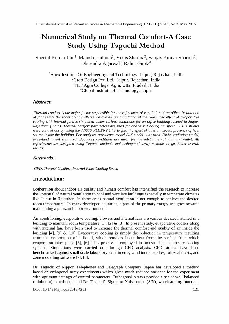
In present study CFD simulation was carried out for four cases of design of office as shown in
figure. Main focus was on air inlet boundary condition of office. In this study a window area 21
inch x 21 inch was used for air inlet conditions based on desert cooler cross section. Office walls
are assumed to be made by brick wall material with insulation at proper places of vertical external
walls. Thickness of walls are assumed 9 inch. Internal partition was made of Aluminium frame
with glass sheets.
Fig 1: Office building under consideration for simulation
Abbreviations and Acronyms:
F13- location of point under fan 1 at 3 feet.
F15- - location of point under fan 1 at 5 feet.
F23- location of point under fan 2 at 3 feet
F25- location of point under fan 2 at 5 feet
F33- location of point under fan 3 at 3 feet
F35- location of point under fan 3 at 5 feet
SN ratio- signal to noise ratio.
Experimental:
CFD modelling Computational fluid dynamics (CFD) is a branch of science which predicts the fluid flow, heat
and mass transfer, chemical reactions, and any other related physical phenomenon. CFD solves
various governing equations for conservation of mass, momentum, energy, turbulence and
International Journal of Recent advances in Mechanical Engineering (IJMECH) Vol.4, No.2, May 2015
123
various other transport state equations. The CFD modelling is done on ANSYS FLUENT 14.5.
CFD modelling solves the mass momentum and energy equations by dividing the solution
domain into many computational cells. CFD modelling provides more accurate results than other
techniques. The Bousinessq assumption was applied to represent the buoyancy force, and the
renormalization group, (RNG) and k-ε model was employed to approximate turbulence. Gan
implemented a parametric investigation of airflow rates in a three-dimensional Trombe wall using
the RNG k-ε model. Basically there are three steps in CFD modelling as follows:
A. Pre-processing:
The major steps involved in pre processing are:
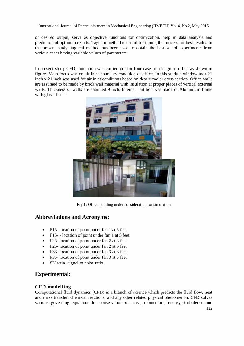
Geometrical details – First of all geometry of the office building was created using Autodesk
Inventor 2014 (a CAD software). The length of the building 35ft. The width of the building 30ft.
The height of the building is 10ft. The figure is shown below.
Fig. 2: Geometrical representation of office building
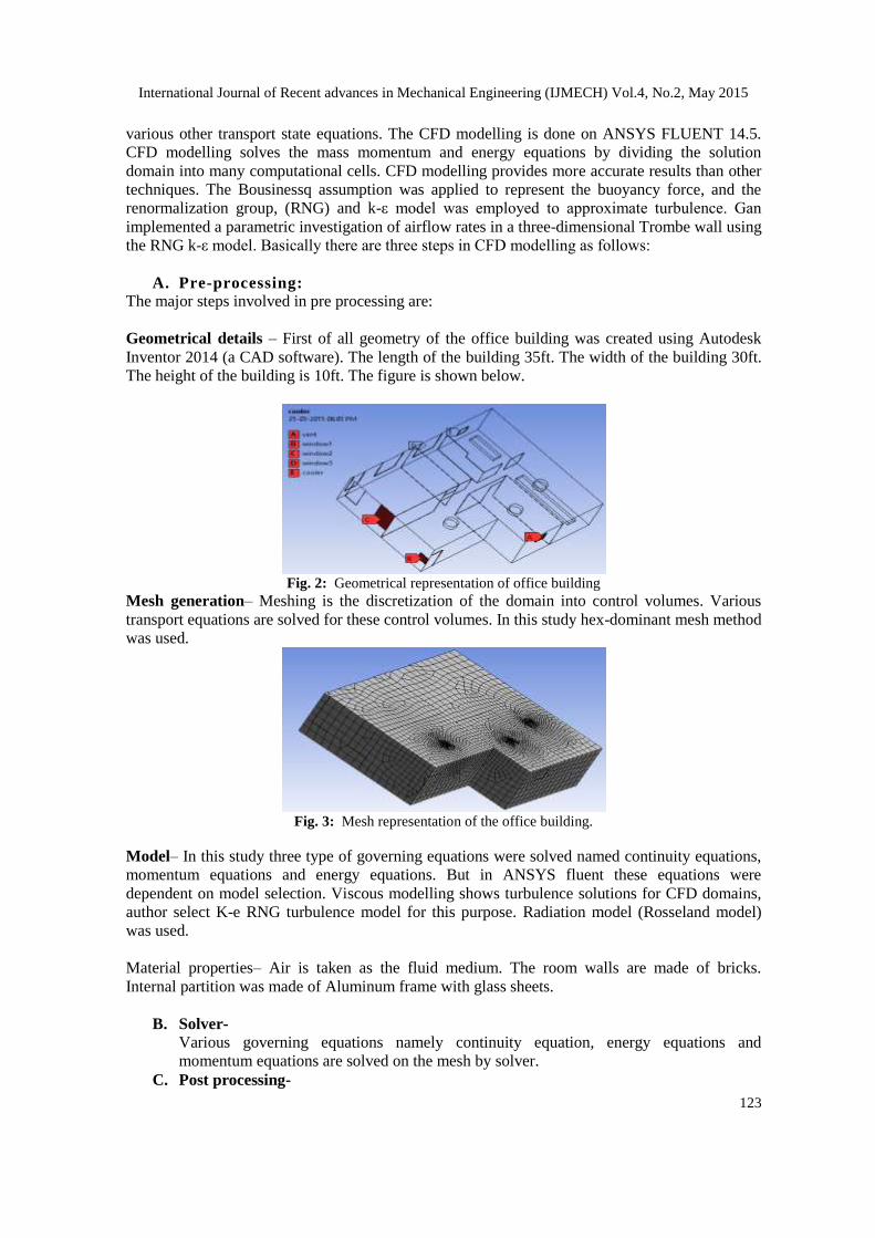
Mesh generation– Meshing is the discretization of the domain into control volumes. Various
transport equations are solved for these control volumes. In this study hex-dominant mesh method
was used.
Fig. 3: Mesh representation of the office building.
Model– In this study three type of governing equations were solved named continuity equations,
momentum equations and energy equations. But in ANSYS fluent these equations were
dependent on model selection. Viscous modelling shows turbulence solutions for CFD domains,
author select K-e RNG turbulence model for this purpose. Radiation model (Rosseland model)
was used.
Material properties– Air is taken as the fluid medium. The room walls are made of bricks.
Internal partition was made of Aluminum frame with glass sheets.
B. Solver-
Various governing equations namely continuity equation, energy equations and
momentum equations are solved on the mesh by solver.
C. Post processing-
International Journal of Recent advances in Mechanical Engineering (IJMECH) Vol.4, No.2, May 2015
124
Under post processing, contours, streamlines and graphs are used to infer the results.
Numerical Simulation and Problem Identification:
According to ANSYS CFD 14.5, it is a complete suite of perfect tools for simulating, analyzing,
optimizing and validating machining products used by various industries. This software addresses
the broadest range of manufacturing issues and design geometry types associated with machining
processes.
There are three stages of the simulation in CFD. The first stage of a Finite Volume (FV) method
based simulation is called “pre-process”. This can be performed by using either the simulation
software itself or one of the Computer-Aided Design (CAD) computer programs such as
Autodesk Inventor, and Auto-cad. The geometric model is then meshed using triangular mesh
elements (automatic mesh generation).To finish this first stage, it is required to set the process
conditions into the simulation software. In the second stage of a simulation process, various
governing equations are performed and applied to a model analysis. The last stage of a FVM
simulation is called “post-process”, where the experience of the analyst is required to extract the
reliable and most important information from multiples coloured contour results offered by the
simulation software Pre-process is very important for the efficiency of the simulation model.
Hence, it must be thoroughly analyzed on the part geometry and its conditions as described in the
following section.
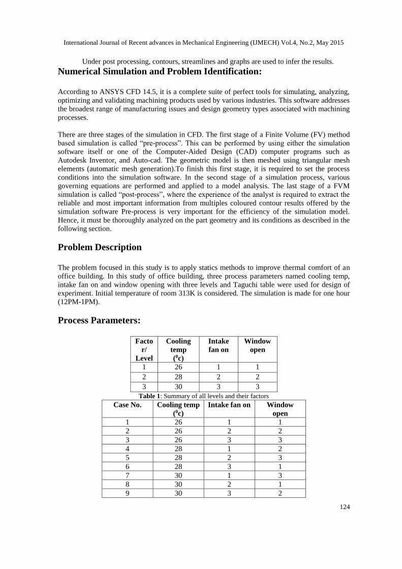
Problem Description
The problem focused in this study is to apply statics methods to improve thermal comfort of an
office building. In this study of office building, three process parameters named cooling temp,
intake fan on and window opening with three levels and Taguchi table were used for design of
experiment. Initial temperature of room 313K is considered. The simulation is made for one hour
(12PM-1PM).
Process Parameters:
Facto
r/
Level
Cooling
temp
(0c)
Intake
fan on
Window
open
1 26 1 1
2 28 2 2
3 30 3 3
Table 1: Summary of all levels and their factors
Case No. Cooling temp
(0c)
Intake fan on Window
open
1 26 1 1
2 26 2 2
3 26 3 3
4 28 1 2
5 28 2 3
6 28 3 1
7 30 1 3
8 30 2 1
9 30 3 2
International Journal of Recent advances in Mechanical Engineering (IJMECH) Vol.4, No.2, May 2015
125
Table 2: orthogonal array Taguchi Table
Results and Discussions
Results are shown for the different cases for temperature and velocity with time which are
simulated by CFD.
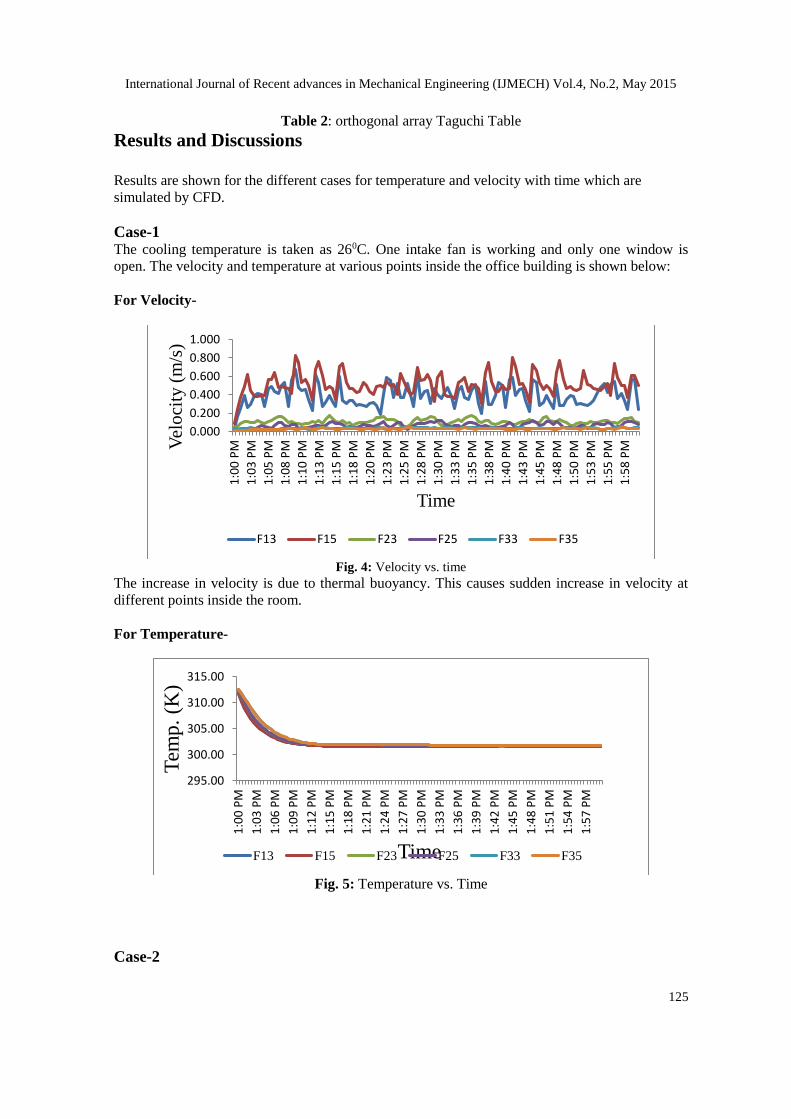
Case-1 The cooling temperature is taken as 260C. One intake fan is working and only one window is
open. The velocity and temperature at various points inside the office building is shown below:
For Velocity-
Fig. 4: Velocity vs. time
The increase in velocity is due to thermal buoyancy. This causes sudden increase in velocity at
different points inside the room.
For Temperature-
Fig. 5: Temperature vs. Time
Case-2
0.000
0.200
0.400
0.600
0.800
1.000
1:0
0 P
M
1:0
3 P
M
1:0
5 P
M
1:0
8 P
M
1:1
0 P
M
1:1
3 P
M
1:1
5 P
M
1:1
8 P
M
1:2
0 P
M
1:2
3 P
M
1:2
5 P
M
1:2
8 P
M
1:3
0 P
M
1:3
3 P
M
1:3
5 P
M
1:3
8 P
M
1:4
0 P
M
1:4
3 P
M
1:4
5 P
M
1:4
8 P
M
1:5
0 P
M
1:5
3 P
M
1:5
5 P
M
1:5
8 P
MVel
oci
ty (
m/s
)
Time
F13 F15 F23 F25 F33 F35
295.00
300.00
305.00
310.00
315.00
1:0
0 P
M
1:0
3 P
M
1:0
6 P
M
1:0
9 P
M
1:1
2 P
M
1:1
5 P
M
1:1
8 P
M
1:2
1 P
M
1:2
4 P
M
1:2
7 P
M
1:3
0 P
M
1:3
3 P
M
1:3
6 P
M
1:3
9 P
M
1:4
2 P
M
1:4
5 P
M
1:4
8 P
M
1:5
1 P
M
1:5
4 P
M
1:5
7 P
M
Tem
p.
(K)
TimeF13 F15 F23 F25 F33 F35
International Journal of Recent advances in Mechanical Engineering (IJMECH) Vol.4, No.2, May 2015
126
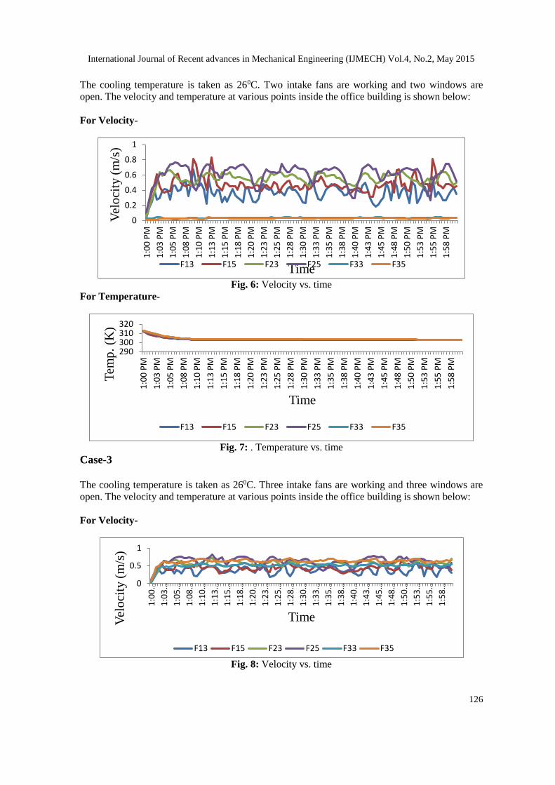
The cooling temperature is taken as 260C. Two intake fans are working and two windows are
open. The velocity and temperature at various points inside the office building is shown below:
For Velocity-
Fig. 6: Velocity vs. time
For Temperature-
Fig. 7: . Temperature vs. time
Case-3
The cooling temperature is taken as 260C. Three intake fans are working and three windows are
open. The velocity and temperature at various points inside the office building is shown below:
For Velocity-
Fig. 8: Velocity vs. time
0
0.2
0.4
0.6
0.8
11
:00
PM
1:0
3 P
M
1:0
5 P
M
1:0
8 P
M
1:1
0 P
M
1:1
3 P
M
1:1
5 P
M
1:1
8 P
M
1:2
0 P
M
1:2
3 P
M
1:2
5 P
M
1:2
8 P
M
1:3
0 P
M
1:3
3 P
M
1:3
5 P
M
1:3
8 P
M
1:4
0 P
M
1:4
3 P
M
1:4
5 P
M
1:4
8 P
M
1:5
0 P
M
1:5
3 P
M
1:5
5 P
M
1:5
8 P
M
Vel
oci
ty (
m/s
)
TimeF13 F15 F23 F25 F33 F35
290300310320
1:0
0 P
M
1:0
3 P
M
1:0
5 P
M
1:0
8 P
M
1:1
0 P
M
1:1
3 P
M
1:1
5 P
M
1:1
8 P
M
1:2
0 P
M
1:2
3 P
M
1:2
5 P
M
1:2
8 P
M
1:3
0 P
M
1:3
3 P
M
1:3
5 P
M
1:3
8 P
M
1:4
0 P
M
1:4
3 P
M
1:4
5 P
M
1:4
8 P
M
1:5
0 P
M
1:5
3 P
M
1:5
5 P
M
1:5
8 P
M
Tem
p.
(K)
Time
F13 F15 F23 F25 F33 F35
0
0.5
1
1:00…
1:03…
1:05…
1:08…
1:10…
1:13…
1:15…
1:18…
1:20…
1:23…
1:25…
1:28…
1:30…
1:33…
1:35…
1:38…
1:40…
1:43…
1:45…
1:48…
1:50…
1:53…
1:55…
1:58…
Vel
oci
ty (
m/s
)
Time
F13 F15 F23 F25 F33 F35
International Journal of Recent advances in Mechanical Engineering (IJMECH) Vol.4, No.2, May 2015
127
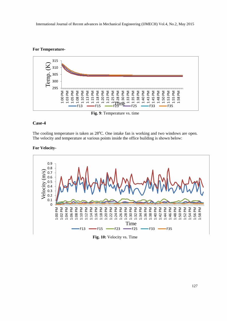
For Temperature-
Fig. 9: Temperature vs. time
Case-4
The cooling temperature is taken as 280C. One intake fan is working and two windows are open.
The velocity and temperature at various points inside the office building is shown below:
For Velocity-
Fig. 10: Velocity vs. Time
295
300
305
310
3151
:00
PM
1:0
3 P
M
1:0
5 P
M
1:0
8 P
M
1:1
0 P
M
1:1
3 P
M
1:1
5 P
M
1:1
8 P
M
1:2
0 P
M
1:2
3 P
M
1:2
5 P
M
1:2
8 P
M
1:3
0 P
M
1:3
3 P
M
1:3
5 P
M
1:3
8 P
M
1:4
0 P
M
1:4
3 P
M
1:4
5 P
M
1:4
8 P
M
1:5
0 P
M
1:5
3 P
M
1:5
5 P
M
1:5
8 P
M
Tem
p.
(K)
TimeF13 F15 F23 F25 F33 F35
00.10.20.30.40.50.60.70.80.9
1:0
0 P
M
1:0
2 P
M
1:0
4 P
M
1:0
6 P
M
1:0
8 P
M
1:1
0 P
M
1:1
2 P
M
1:1
4 P
M
1:1
6 P
M
1:1
8 P
M
1:2
0 P
M
1:2
2 P
M
1:2
4 P
M
1:2
6 P
M
1:2
8 P
M
1:3
0 P
M
1:3
2 P
M
1:3
4 P
M
1:3
6 P
M
1:3
8 P
M
1:4
0 P
M
1:4
2 P
M
1:4
4 P
M
1:4
6 P
M
1:4
8 P
M
1:5
0 P
M
1:5
2 P
M
1:5
4 P
M
1:5
6 P
M
1:5
8 P
M
Vel
oci
ty (
m/s
)
TimeF13 F15 F23 F25 F33 F35
International Journal of Recent advances in Mechanical Engineering (IJMECH) Vol.4, No.2, May 2015
128
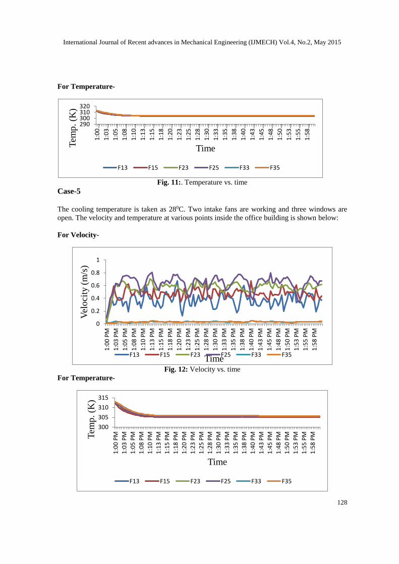
For Temperature-
Fig. 11:. Temperature vs. time
Case-5
The cooling temperature is taken as 280C. Two intake fans are working and three windows are
open. The velocity and temperature at various points inside the office building is shown below:
For Velocity-
Fig. 12: Velocity vs. time
For Temperature-
290300310320
1:00…
1:03…
1:05…
1:08…
1:10…
1:13…
1:15…
1:18…
1:20…
1:23…
1:25…
1:28…
1:30…
1:33…
1:35…
1:38…
1:40…
1:43…
1:45…
1:48…
1:50…
1:53…
1:55…
1:58…
Tem
p.
(K)
Time
F13 F15 F23 F25 F33 F35
0
0.2
0.4
0.6
0.8
1
1:0
0 P
M
1:0
3 P
M
1:0
5 P
M
1:0
8 P
M
1:1
0 P
M
1:1
3 P
M
1:1
5 P
M
1:1
8 P
M
1:2
0 P
M
1:2
3 P
M
1:2
5 P
M
1:2
8 P
M
1:3
0 P
M
1:3
3 P
M
1:3
5 P
M
1:3
8 P
M
1:4
0 P
M
1:4
3 P
M
1:4
5 P
M
1:4
8 P
M
1:5
0 P
M
1:5
3 P
M
1:5
5 P
M
1:5
8 P
M
Vel
oci
ty (
m/s
)
TimeF13 F15 F23 F25 F33 F35
300
305
310
315
1:0
0 P
M
1:0
3 P
M
1:0
5 P
M
1:0
8 P
M
1:1
0 P
M
1:1
3 P
M
1:1
5 P
M
1:1
8 P
M
1:2
0 P
M
1:2
3 P
M
1:2
5 P
M
1:2
8 P
M
1:3
0 P
M
1:3
3 P
M
1:3
5 P
M
1:3
8 P
M
1:4
0 P
M
1:4
3 P
M
1:4
5 P
M
1:4
8 P
M
1:5
0 P
M
1:5
3 P
M
1:5
5 P
M
1:5
8 P
MTem
p.
(K)
Time
F13 F15 F23 F25 F33 F35
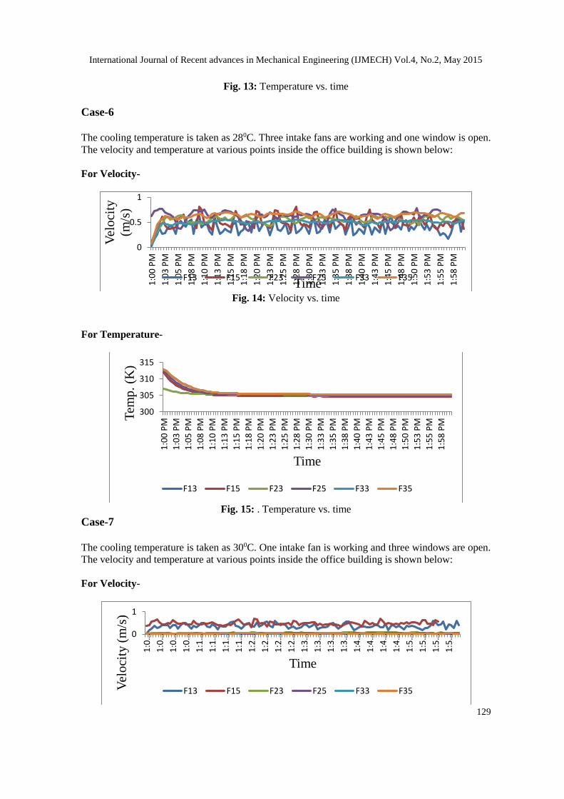
International Journal of Recent advances in Mechanical Engineering (IJMECH) Vol.4, No.2, May 2015
129
Fig. 13: Temperature vs. time
Case-6
The cooling temperature is taken as 280C. Three intake fans are working and one window is open.
The velocity and temperature at various points inside the office building is shown below:
For Velocity-
Fig. 14: Velocity vs. time
For Temperature-
Fig. 15: . Temperature vs. time
Case-7
The cooling temperature is taken as 300C. One intake fan is working and three windows are open.
The velocity and temperature at various points inside the office building is shown below:
For Velocity-
0
0.5
1
1:0
0 P
M
1:0
3 P
M
1:0
5 P
M
1:0
8 P
M
1:1
0 P
M
1:1
3 P
M
1:1
5 P
M
1:1
8 P
M
1:2
0 P
M
1:2
3 P
M
1:2
5 P
M
1:2
8 P
M
1:3
0 P
M
1:3
3 P
M
1:3
5 P
M
1:3
8 P
M
1:4
0 P
M
1:4
3 P
M
1:4
5 P
M
1:4
8 P
M
1:5
0 P
M
1:5
3 P
M
1:5
5 P
M
1:5
8 P
M
Vel
oci
ty
(m/s
)
TimeF13 F15 F23 F25 F33 F35
300
305
310
315
1:0
0 P
M
1:0
3 P
M
1:0
5 P
M
1:0
8 P
M
1:1
0 P
M
1:1
3 P
M
1:1
5 P
M
1:1
8 P
M
1:2
0 P
M
1:2
3 P
M
1:2
5 P
M
1:2
8 P
M
1:3
0 P
M
1:3
3 P
M
1:3
5 P
M
1:3
8 P
M
1:4
0 P
M
1:4
3 P
M
1:4
5 P
M
1:4
8 P
M
1:5
0 P
M
1:5
3 P
M
1:5
5 P
M
1:5
8 P
M
Tem
p.
(K)
Time
F13 F15 F23 F25 F33 F35
0
1
1:0…
1:0…
1:0…
1:0…
1:1…
1:1…
1:1…
1:1…
1:2…
1:2…
1:2…
1:2…
1:3…
1:3…
1:3…
1:3…
1:4…
1:4…
1:4…
1:4…
1:5…
1:5…
1:5…
1:5…
Vel
oci
ty (
m/s
)
Time
F13 F15 F23 F25 F33 F35
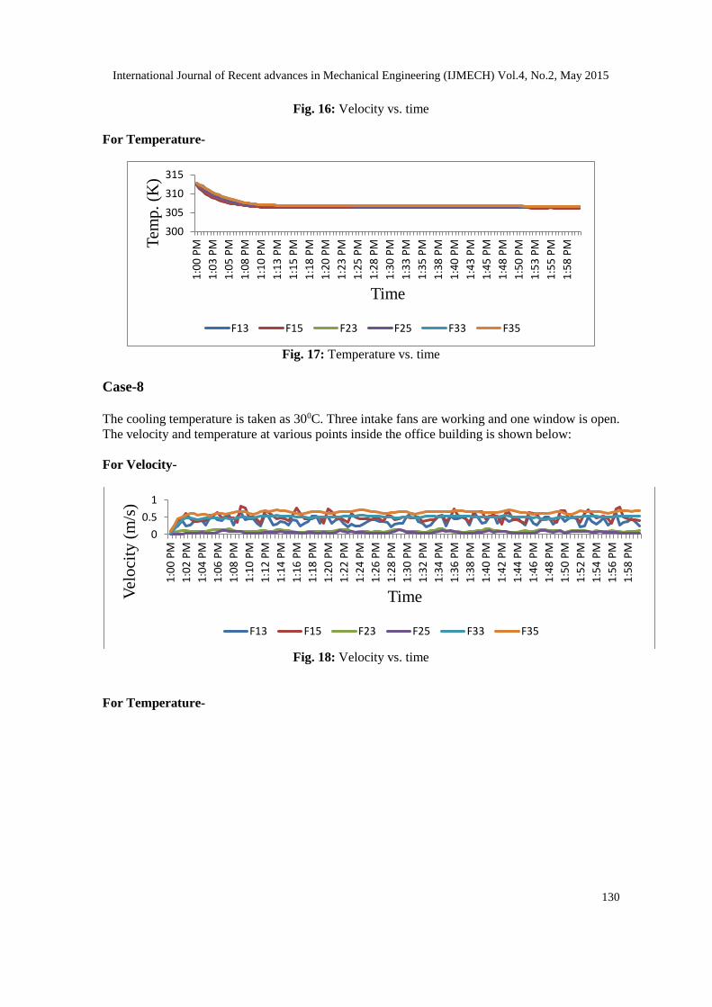
International Journal of Recent advances in Mechanical Engineering (IJMECH) Vol.4, No.2, May 2015
130
Fig. 16: Velocity vs. time
For Temperature-
Fig. 17: Temperature vs. time
Case-8
The cooling temperature is taken as 300C. Three intake fans are working and one window is open.
The velocity and temperature at various points inside the office building is shown below:
For Velocity-
Fig. 18: Velocity vs. time
For Temperature-
300
305
310
315
1:0
0 P
M
1:0
3 P
M
1:0
5 P
M
1:0
8 P
M
1:1
0 P
M
1:1
3 P
M
1:1
5 P
M
1:1
8 P
M
1:2
0 P
M
1:2
3 P
M
1:2
5 P
M
1:2
8 P
M
1:3
0 P
M
1:3
3 P
M
1:3
5 P
M
1:3
8 P
M
1:4
0 P
M
1:4
3 P
M
1:4
5 P
M
1:4
8 P
M
1:5
0 P
M
1:5
3 P
M
1:5
5 P
M
1:5
8 P
MTem
p.
(K)
Time
F13 F15 F23 F25 F33 F35
0
0.5
1
1:0
0 P
M
1:0
2 P
M
1:0
4 P
M
1:0
6 P
M
1:0
8 P
M
1:1
0 P
M
1:1
2 P
M
1:1
4 P
M
1:1
6 P
M
1:1
8 P
M
1:2
0 P
M
1:2
2 P
M
1:2
4 P
M
1:2
6 P
M
1:2
8 P
M
1:3
0 P
M
1:3
2 P
M
1:3
4 P
M
1:3
6 P
M
1:3
8 P
M
1:4
0 P
M
1:4
2 P
M
1:4
4 P
M
1:4
6 P
M
1:4
8 P
M
1:5
0 P
M
1:5
2 P
M
1:5
4 P
M
1:5
6 P
M
1:5
8 P
M
Vel
oci
ty (
m/s
)
Time
F13 F15 F23 F25 F33 F35
International Journal of Recent advances in Mechanical Engineering (IJMECH) Vol.4, No.2, May 2015
131
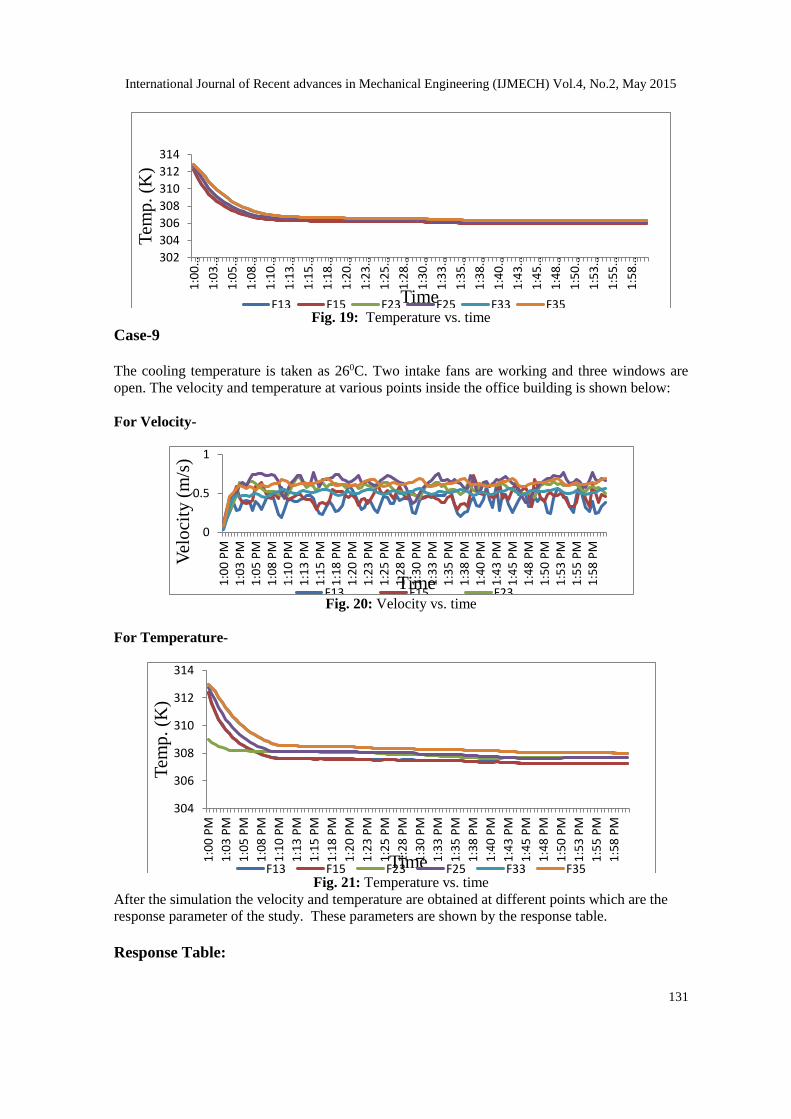
Fig. 19: Temperature vs. time
Case-9
The cooling temperature is taken as 260C. Two intake fans are working and three windows are
open. The velocity and temperature at various points inside the office building is shown below:
For Velocity-
Fig. 20: Velocity vs. time
For Temperature-
Fig. 21: Temperature vs. time
After the simulation the velocity and temperature are obtained at different points which are the
response parameter of the study. These parameters are shown by the response table.
Response Table:
302
304
306
308
310
312
314
1:00…
1:03…
1:05…
1:08…
1:10…
1:13…
1:15…
1:18…
1:20…
1:23…
1:25…
1:28…
1:30…
1:33…
1:35…
1:38…
1:40…
1:43…
1:45…
1:48…
1:50…
1:53…
1:55…
1:58…
Tem
p.
(K)
TimeF13 F15 F23 F25 F33 F35
0
0.5
1
1:0
0 P
M1
:03
PM
1:0
5 P
M1
:08
PM
1:1
0 P
M1
:13
PM
1:1
5 P
M1
:18
PM
1:2
0 P
M1
:23
PM
1:2
5 P
M1
:28
PM
1:3
0 P
M1
:33
PM
1:3
5 P
M1
:38
PM
1:4
0 P
M1
:43
PM
1:4
5 P
M1
:48
PM
1:5
0 P
M1
:53
PM
1:5
5 P
M1
:58
PM
Vel
oci
ty (
m/s
)
TimeF13 F15 F23
304
306
308
310
312
314
1:0
0 P
M
1:0
3 P
M
1:0
5 P
M
1:0
8 P
M
1:1
0 P
M
1:1
3 P
M
1:1
5 P
M
1:1
8 P
M
1:2
0 P
M
1:2
3 P
M
1:2
5 P
M
1:2
8 P
M
1:3
0 P
M
1:3
3 P
M
1:3
5 P
M
1:3
8 P
M
1:4
0 P
M
1:4
3 P
M
1:4
5 P
M
1:4
8 P
M
1:5
0 P
M
1:5
3 P
M
1:5
5 P
M
1:5
8 P
M
Tem
p.
(K)
TimeF13 F15 F23 F25 F33 F35
International Journal of Recent advances in Mechanical Engineering (IJMECH) Vol.4, No.2, May 2015
132
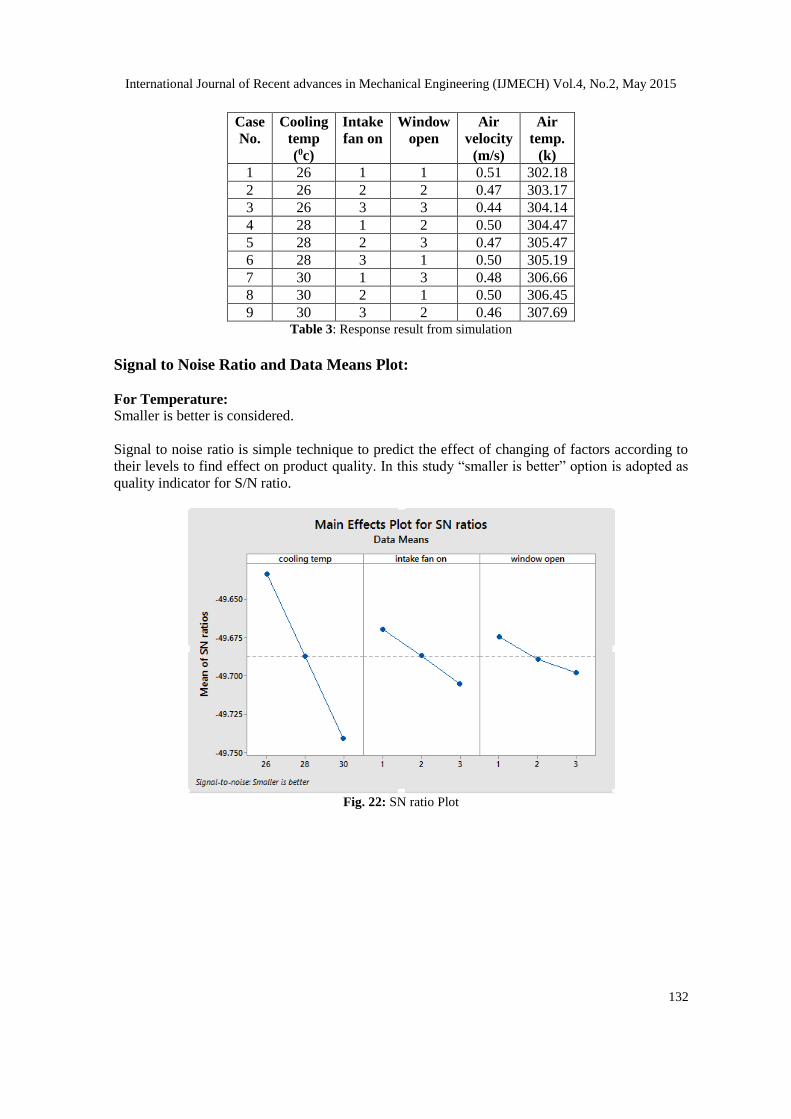
Case
No.
Cooling
temp
(0c)
Intake
fan on
Window
open
Air
velocity
(m/s)
Air
temp.
(k)
1 26 1 1 0.51 302.18
2 26 2 2 0.47 303.17
3 26 3 3 0.44 304.14
4 28 1 2 0.50 304.47
5 28 2 3 0.47 305.47
6 28 3 1 0.50 305.19
7 30 1 3 0.48 306.66
8 30 2 1 0.50 306.45
9 30 3 2 0.46 307.69 Table 3: Response result from simulation
Signal to Noise Ratio and Data Means Plot:
For Temperature:
Smaller is better is considered.
Signal to noise ratio is simple technique to predict the effect of changing of factors according to
their levels to find effect on product quality. In this study “smaller is better” option is adopted as
quality indicator for S/N ratio.
Fig. 22: SN ratio Plot
International Journal of Recent advances in Mechanical Engineering (IJMECH) Vol.4, No.2, May 2015
133
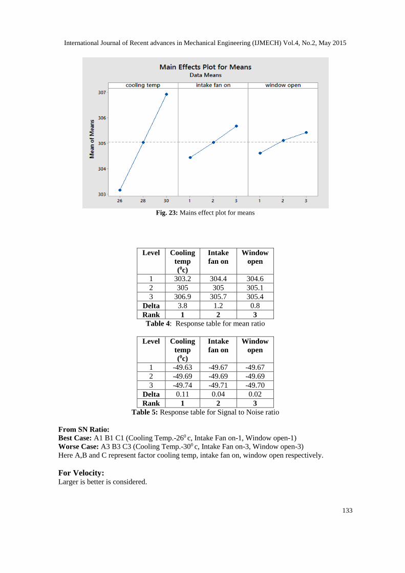
Fig. 23: Mains effect plot for means
Level Cooling
temp
(0c)
Intake
fan on
Window
open
1 303.2 304.4 304.6
2 305 305 305.1
3 306.9 305.7 305.4
Delta 3.8 1.2 0.8
Rank 1 2 3
Table 4: Response table for mean ratio
Level Cooling
temp
(0c)
Intake
fan on
Window
open
1 -49.63 -49.67 -49.67
2 -49.69 -49.69 -49.69
3 -49.74 -49.71 -49.70
Delta 0.11 0.04 0.02
Rank 1 2 3
Table 5: Response table for Signal to Noise ratio
From SN Ratio:
Best Case: A1 B1 C1 (Cooling Temp.-260 c, Intake Fan on-1, Window open-1)
Worse Case: A3 B3 C3 (Cooling Temp.-300 c, Intake Fan on-3, Window open-3)
Here A,B and C represent factor cooling temp, intake fan on, window open respectively.
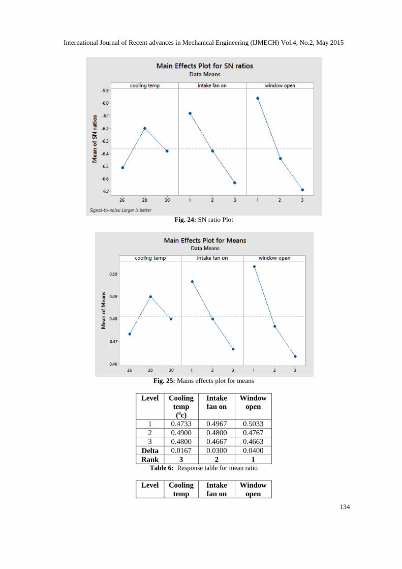
For Velocity: Larger is better is considered.
International Journal of Recent advances in Mechanical Engineering (IJMECH) Vol.4, No.2, May 2015
134
Fig. 24: SN ratio Plot
Fig. 25: Mains effects plot for means
Level Cooling
temp
(0c)
Intake
fan on
Window
open
1 0.4733 0.4967 0.5033
2 0.4900 0.4800 0.4767
3 0.4800 0.4667 0.4663
Delta 0.0167 0.0300 0.0400
Rank 3 2 1 Table 6: Response table for mean ratio
Level Cooling
temp
Intake
fan on
Window
open

International Journal of Recent advances in Mechanical Engineering (IJMECH) Vol.4, No.2, May 2015
135
(0c)
1 -6.513 -6.081 -5.963
2 -6.200 -6.379 -6.441
3 -6.380 -6.632 -6.688
Delta 0.313 0.551 0.725
Rank 3 2 1
Table 7: Response table for Signal to Noise ratio
From SN Ratio:
Best Case: A2 B1 C1 (Cooling Temp.-280 c, Intake Fan on-1, Window open-1)
Worse Case: A1 B3 C3 (Cooling Temp.-260 c, Intake Fan on-3, Window open-3)
Here A,B and C represent factor cooling temp, intake fan on, window open respectively.
Conclusion:
A good agreement is observed by the CFD analysis of an office building using Taguchi method.
It has been observed from all the graphs that the temperature is uniformly decrease but in velocity
there is continuously variation. There were three levels and three factors. In total, nine cases were
simulated and it is concluded that the best case for the thermal comfort of the building according
to temperature is when the cooling temperature is 260C, and only one window is open and only
one intake fan is on. Also from the response table above, it is concluded that the cooling
temperature is the important factor among other factors for thermal comfort and best case
according to velocity is when the cooling temperature is 280c, and only one intake fan & one
window open.
Future Scope More convenient design tools and software can be used for this study which can provide the
better thermal comfort results. Fuzzy logic can be used in this study which can provide comfort at
minimum energy use. Ergonomics can be taken into consideration which determines
metabolic heat production, an essential requirement and the assessment of thermal
comfort.
References:
[1] Al-Rashidi Khaled, Loveday Dennis and Al-Mutawa Nawaf Impact of ventilation modes on
carbon dioxide concentration levels in Kuwait classrooms [Journal] // Energy and Buildings.
- 2012. - Vol. 87. - pp. 540-549.
[2] Barbason Mathieu and Reiter Sigrid Coupling building energy simulation and computational
fluid dynamics: Application to a two-storey house in a temperate climate [Journal] //
Building and Environment. - 2014. - Vol. 75. - pp. 30-39.
[3] Borge-Diez David [et al.] Passive climatization using a cool roof and natural ventilation for
internally displaced persons in hot climates: Case study for Haiti [Journal] // Building and
Environment. - 2013. - Vol. 59. - pp. 116-126.
[4] Caciolo Marcello [et al.] Development of a new correlation for single-sided natural
ventilation adapted to leeward conditions [Journal] // Energy and Buildings. - 2013. - Vol.
60. - pp. 372-382.
International Journal of Recent advances in Mechanical Engineering (IJMECH) Vol.4, No.2, May 2015
136
[5] Zhang Lin, T.T. Chow, C.F. Tsang, 9 November 2005, Effect of door opening on the
performance of displacement ventilation in a typical office building.
[6] Fan Jianhua, Hviid Christian Anker and Honglu Yang Performance analysis of a new design
of office diffuse ceiling ventilation system [Journal] // Energy and Buildings. - 2013. - Vol.
59. - pp. 73-81.
[7] Gloriant François [et al.] Modeling a triple-glazed supply-air window [Journal] // Building
and Environment. - 2014. - Vol. 84. - pp. 1-9.
[8] Hajdukiewicz Magdalena, Geron Marco and Keane Marcus M. Calibrated CFD simulation
to evaluate thermal comfort in a highly-glazed naturally ventilated room [Journal] //
Building and Environment. - 2013. - Vol. 70. - pp. 73-89.
[9] Hirano Tomoko [et al.] A study on a porous residential building model in hot and humid
regions: Part 1—the natural ventilation performance and the cooling load reduction effect of
the building model [Journal] // Building and Environment. - 2006. - Vol. 41. - pp. 21-32.
[10 ]Cruz-Salas M.V., J.A.Castillo and G.Huelsz Experimental study on natural ventilation of a
room with a windward window and different wind exchanger [Journal] // Energy and
Buildings. - 2014. - Vol. 84. - pp. 458-465.