numerical studies of the klein-gordon-schrodinger˜ equations
TRANSCRIPT

NUMERICAL STUDIES OF THE
KLEIN-GORDON-SCHRODINGER
EQUATIONS
LI YANG
(M.Sc., Sichuan University)
A THESIS SUBMITTED
FOR THE DEGREE OF MASTER OF SCIENCE
DEPARTMENT OF MATHEMATICS
NATIONAL UNIVERSITY OF SINGAPORE
2006

Acknowledgements
I would like to thank my advisor, Associate Professor Bao Weizhu, who gave me
the opportunity to work on such an interesting research project, paid patient guid-
ance to me, reviewed my thesis and gave me much invaluable help and constructive
suggestions on it.
It is also my pleasure to express my appreciation and gratitude to Zhang Yanzhi,
Wang Hanquan, and Lim Fongyin, from whom I got valuable suggestions and great
help on my research project.
I would also wish to thank the National University of Singapore for her financial
support by awarding me the Research Scholarship during the period of my MSc
candidature.
My sincere thanks go to the Mathematics Department of NUS for its kind help
during my two-year study here.
Li Yang
June 2006
ii
Contents
Acknowledgements ii
Summary vi
List of Tables ix
List of Figures x
1 Introduction 1
1.1 Physical background . . . . . . . . . . . . . . . . . . . . . . . . . . . 1
1.2 The problem . . . . . . . . . . . . . . . . . . . . . . . . . . . . . . . . 2
1.3 Contemporary studies . . . . . . . . . . . . . . . . . . . . . . . . . . 3
1.4 Overview of our work . . . . . . . . . . . . . . . . . . . . . . . . . . . 5
2 Numerical studies of the Klein-Gordon equation 8
2.1 Derivation of the Klein-Gordon equation . . . . . . . . . . . . . . . . 8
2.2 Conservation laws of the Klein-Gordon equation . . . . . . . . . . . . 10
2.3 Numerical methods for the Klein-Gordon equation . . . . . . . . . . . 12
iii

Contents iv
2.3.1 Existing numerical methods . . . . . . . . . . . . . . . . . . . 13
2.3.2 Our new numerical method . . . . . . . . . . . . . . . . . . . 14
2.4 Numerical results of the Klein-Gordon equation . . . . . . . . . . . . 15
2.4.1 Comparison of different methods . . . . . . . . . . . . . . . . 15
2.4.2 Applications of CN-LF-SP . . . . . . . . . . . . . . . . . . . . 18
3 The Klein-Gordon-Schrodinger equations 26
3.1 Derivation of the Klein-Gordon-Schrodinger equations . . . . . . . . . 26
3.2 Conservation laws of the Klein-Gordon-Schrodinger equations . . . . 28
3.3 Dynamics of mean value of the meson field . . . . . . . . . . . . . . . 30
3.4 Plane wave and soliton wave solutions of KGS . . . . . . . . . . . . . 31
3.5 Reduction to the Schrodinger-Yukawa equations (S-Y) . . . . . . . . 32
4 Numerical studies of the Klein-Gordon-Schrodinger equations 34
4.1 Numerical methods for the Klein-Gordon-Schrodinger equations . . . 34
4.1.1 Time-splitting for the nonlinear Schrodinger equation . . . . . 36
4.1.2 Phase space analytical solver+time-splitting spectral discretiza-
tions (PSAS-TSSP) . . . . . . . . . . . . . . . . . . . . . . . . 36
4.1.3 Crank-Nicolson leap-frog time-splitting spectral discretizations
(CN-LF-TSSP) . . . . . . . . . . . . . . . . . . . . . . . . . . 40
4.2 Properties of numerical methods . . . . . . . . . . . . . . . . . . . . . 42
4.2.1 For plane wave solution . . . . . . . . . . . . . . . . . . . . . 42
4.2.2 Conservation and decay rate . . . . . . . . . . . . . . . . . . . 43
4.2.3 Dynamics of mean value of meson field . . . . . . . . . . . . . 45
4.2.4 Stability analysis . . . . . . . . . . . . . . . . . . . . . . . . . 49
4.3 Numerical results of the Klein-Gordon-Schrodinger equation . . . . . 52
4.3.1 Comparisons of different methods . . . . . . . . . . . . . . . . 52

Contents v
4.3.2 Application of our numerical methods . . . . . . . . . . . . . . 57
5 Application to the Schrodinger-Yukawa equations 70
5.1 Introduction to the Schrodinger-Yukawa equations . . . . . . . . . . . 70
5.2 Numerical method for the Schrodinger-Yukawa equations . . . . . . . 72
5.3 Numerical results of the Schrodinger-Yukawa equations . . . . . . . . 73
5.3.1 Convergence of KGS to S-Y in “nonrelativistic limit” regime . 73
5.3.2 Applications . . . . . . . . . . . . . . . . . . . . . . . . . . . . 74
6 Conclusion 78

Summary
In this thesis, we present a numerical method for the nonlinear Klein-Gordon equa-
tion and two numerical methods for studying solutions of the Klein-Gordon-Schrodinger
equations.We begin with the derivation of the Klein-Gordon equation (KG) which
describes scalar (or pseudoscalar) spinless particles, analyze its properties and present
Crank-Nicolson leap-frog spectral method (CN-LF-SP) for numerical discretization
of the nonlinear Klein-Gordon equation. Numerical results for the Klein-Gordon
equation demonstrat that the method is of spectral-order accuracy in space and
second-order accuracy in time and it is much better than the other numerical meth-
ods proposed in the literature. It also preserves the system energy, linear mo-
mentum and angular momentum very well in the discretized level. We continue
with the derivation of the Klein-Gordon-Schrodinger equations (KGS) which de-
scribes a system of conserved scalar nucleons interacting with neutral scalar mesons
coupled through the Yukawa interaction and analyze its properties. Two efficient
and accurate numerical methods are proposed for numerical discretization of the
Klein-Gordon-Schrodinger equations. They are phase space analytical solver+time-
splitting spectral method (PSAS-TSSP) and Crank-Nicolson leap-frog time-splitting
spectral method (CN-LF-TSSP). These methods are explicit, unconditionally sta-
ble, of spectral accuracy in space and second order accuracy in time, easy to extend
vi

Summary vii
to high dimensions, easy to program, less memory-demanding, and time reversible
and time transverse invariant. Furthermore, they conserve (or keep the same decay
rate of) the wave energy in KGS when there is no damping (or a linear damping)
term, give exact results for plane-wave solutions of KGS, and keep the same dy-
namics of the mean value of the meson field in discretized level. We also apply our
new numerical methods to study numerically soliton-soliton interaction of KGS in
1D and dynamics of KGS in 2D. We numerically find that, when a large damping
term is added to the Klein-Gordon equation, bound state of KGS can be obtained
from the dynamics of KGS when time goes to infinity. Finally, we extend our nu-
merical method, time-splitting spectral method (TSSP) to the Schrodinger-Yukawa
equations and present the numerical results of the Schrodinger-Yukawa equations in
1D and 2D cases.
The thesis is organized as follows: Chapter 1 introduces the physical background of
the Klein-Gordon equation and the Klein-Gordon-Schrodinger equations. We also
review some existing results of them and report our main results. In Chapter 2, the
Klein-Gordon equation, which describes scalar (or pseudoscalar) spinless particles,
is derived and its analytical properties are analyzed. The Crank-Nicolson leap-frog
spectral method for the nonlinear Klein-Gordon equation is presented and other
existing numerical methods are introduced. We also report the numerical results
of the nonlinear Klein-Gordon equation, i.e., the breather solution of KG, soliton-
soliton collision in 1D and 2D problems. In Chapter 3, the Klein-Gordon-Schrodinger
equations, describing a system of conserved scalar nucleons interacting with neutral
scalar mesons coupled through the Yukawa interaction, is derived and its analytical
properties are analyzed. In Chapter 4, two new efficient and accurate numerical
methods are proposed to discretize KGS and the properties of these two numerical
methods are studied. We test the accuracy and stability of our methods for KGS
with a solitary wave solution, and apply them to study numerically dynamics of a
plane wave, soliton-soliton collision in 1D with/without damping terms and a 2D

Summary viii
problem of KGS. In Chapter 5, we extend our methods to the Schrodinger-Yukawa
equations and report some numerical results of them. Finally, some conclusions
based on our findings and numerical results are drawn in Chapter 6.

List of Tables
2.1 Spatial discretization errors e(t) at time t = 1 for different mesh sizes
h under k = 0.001. . . . . . . . . . . . . . . . . . . . . . . . . . . . . 18
2.2 Temporal discretization errors e(t) at time t = 1 for different time
steps k under h = 1/16. . . . . . . . . . . . . . . . . . . . . . . . . . 18
2.3 Conserved quantities analysis: k = 0.001 and h = 1/16. . . . . . . . . 19
4.1 Spatial discretization errors e1(t) and e2(t) at time t = 2 for different
mesh sizes h under k = 0.0001. I: For γ = 0. . . . . . . . . . . . . . . 53
4.1 (cont’d): II: For γ = 0.5. . . . . . . . . . . . . . . . . . . . . . . . . . 54
4.2 Temporal discretization errors e1(t) and e2(t) at time t = 1 for differ-
ent time steps k. I: For γ = 0. . . . . . . . . . . . . . . . . . . . . . . 55
4.2 (cont’d): II. For γ = 0.5 and h = 1/4. . . . . . . . . . . . . . . . . . . 56
4.3 Conserved quantities analysis: k = 0.0001 and h = 18. . . . . . . . . . 56
5.1 Error analysis between KGS and its reduction S-Y: Errors are com-
puted at time t = 1 under h = 5/128 and k = 0.00005. . . . . . . . . 74
ix

List of Figures
2.1 Time evolution of soliton-soliton collision in Example 2.1. a): surface
plot; b): contour plot. . . . . . . . . . . . . . . . . . . . . . . . . . . 17
2.2 Time evolution of a stationary Klein-Gordon’s breather solution in
Example 2.2. a): surface plot; b): contour plot. . . . . . . . . . . . . 20
2.3 Circular and elliptic ring solitons in Example 2.3 (from top to bottom:
t = 0, 4, 8, 11.5 and 15). . . . . . . . . . . . . . . . . . . . . . . . . . 23
2.4 Collision of two ring solitons in Example 2.4 (from top to bottom :
t = 0, 2, 4, 6 and 8). . . . . . . . . . . . . . . . . . . . . . . . . . . . 24
2.5 Collision of four ring solitons in Example 2.5 (from top to bottom:
t = 0, 2.5, 5, 7.5 and 10). . . . . . . . . . . . . . . . . . . . . . . . . . 25
4.1 Numerical solutions of the meson field φ (left column) and the nucleon
density |ψ|2 (right column) at t = 1 for Example 1 with Type 1 initial
data in the “nonrelativistic” limit regime by PSAS-TSSP. ’-’: exact
solution given in (4.96), ‘+ + +’: numerical solution. I. With the
meshing strategy h = O(ε) and k = O(ε): (a) Γ0 = (ε0, h0, k0) =
(0.125, 0.25, 0.04), (b) Γ0/4, and (c) Γ0/16. . . . . . . . . . . . . . . . 58
x

List of Figures xi
4.1 (cont’d): II. With the meshing strategy h = O(ε) and k = 0.04-
independent of ε: (d) Γ0 = (ε0, h0) = (0.125, 0.25), (e) Γ0/4, and (f)
Γ0/16. . . . . . . . . . . . . . . . . . . . . . . . . . . . . . . . . . . . 59
4.2 Numerical solutions of the density |ψ(x, t)|2 and the meson field φ(x, t)
at t = 1 in the nonrelativistic limit regime by PSAS-TSSP with the
same mesh (h = 1/2 and k = 0.005). ’-’: ‘exact’ solution , ’+ + +’:
numerical solution. The left column corresponds to the meson field
φ(x, t): (a) ε = 1/2, (c) ε = 1/16. (e) ε = 1/128. The right column
corresponds to the density |ψ(x, t)|2: (b) ε = 1/2, (d) ε = 1/16. (f)
ε = 1/128. . . . . . . . . . . . . . . . . . . . . . . . . . . . . . . . . . 60
4.3 Numerical solutions for plane wave of KGS in Example 4.2 at time
t = 2 (left coumn) and t = 4 (right column). ’–’: exact solution given
in (4.96), ’+ + +’: numerical solution. (a): Real part of nucleon
filed Re(ψ(x, t)); (b): imaginary part of nucleon field Im(ψ(x, t));
(c): meson filed φ. . . . . . . . . . . . . . . . . . . . . . . . . . . . . 61
4.4 Numerical solutions of soliton-soliton collison in standard KGS in
Example 4.3 I: Nucleon density |ψ(x, t)|. . . . . . . . . . . . . . . . . 62
4.5 (cont’d): II. Meson field φ(x, t). . . . . . . . . . . . . . . . . . . . . . 63
4.6 Time evolution of nucleon density |ψ(x, t)|2 (left column) and me-
son field φ(x, t) (right column) for soliton-soliton collision of KGS in
Example 4.4 for different values of γ. . . . . . . . . . . . . . . . . . . 65
4.7 Time evolution of the Hamiltonian H(t) (‘left’) and mean value of
the meson field N(t) (‘right’) in Example 4.4 for different values of γ. 66
4.8 Time evolution of the Hamiltonian H(t) (‘left’) and mean value of
the meson field N(t) (‘right’) in Example 4.6 for different values of γ. 66
4.9 Numerical solutions of the nucleon density |ψ(x, y, t)|2 (right column)
and meson field φ(x, y, t) (left column) in Example 4.5 at t = 1. 1th
row: ε = 1/2; 2nd row: ε = 1/8; 3rd row : ε = 1/32. . . . . . . . . . . 67

List of Figures xii
4.10 Numerical solutions of the nucleon density |ψ(x, y, t)|2 (right column)
and meson field φ(x, y, t) (left column) in Example 4.5 at t = 2. 1th
row: ε = 1/2; 2nd row: ε = 1/8; 3rd row : ε = 1/32. . . . . . . . . . . 68
4.11 Surface plots of the nucleon density |ψ(x, y, t)|2 (left column) and
meson field φ(x, y, t) (right column) in Example 4.6 with γ = 0 at
different times. . . . . . . . . . . . . . . . . . . . . . . . . . . . . . . 69
5.1 Numerical results for different scales of the Xα term in Example 5.2,
i.e., α = 1,√
ε, ε, 0. a) and b) : small time t = 0.25, pre-break, a)
for ε = 0.05, b) for ε = 0.0125. c)-f): large time, t = 4.0, post-break.
c) for ε = 0.1, d) for ε = 0.05, e) for ε = 0.0375, f) ε = 0.025. . . . . . 76
5.2 Time evolution of the position density for Xα term at O(1) in Exam-
ple 5.2, i.e., α = 0.5, with ε = 0.025, h = 1/512 and k = 0.0005. a)
surface plot; b) pseudocolor plot. . . . . . . . . . . . . . . . . . . . . 77
5.3 Time evolution of the position density for attractive Hartree interac-
tion in Example 5.2. C = −1, α = 0.5, ε = 0.025, k = 0.00015. a)
surface plot; b) pseudocolor plot. . . . . . . . . . . . . . . . . . . . . 77

Chapter 1Introduction
In this chapter, we introduce the physical background of the nonlinear Klein-Gordon
equation (KG) and the Klein-Gordon-Schroding equations (KGS) and review some
existing analytical and numerical results of them and report our main results of
these two problems.
1.1 Physical background
The Klein-Gordon equation (or Klein-Fock-Gordon equation) is a relativistic version
of the Schrodinger equation, which describes scalar (or pseudoscalar) spinless parti-
cles. The Klein-Gordon equation was actually first found by Schodinger, before he
made the discovery of the equation that now bears his name. He rejected it because
he couldn’t make it fit the data (the equation doesn’t take into account the spin of
the electron); the way he found his equation was by making simplification in the
Klein-Gordon equation. Later, it was revived and it has become commonly accepted
that Klein-Gordon equation is the appropriate model to describe the wave function
of the particle that is charge-neutral, spinless and relativistic effects can’t be ignored.
It has important applications in plasma physics, together with Zakharov equation
describing the interaction of Langmuir wave and the ion acoustic wave in a plasma
1

1.2 The problem 2
[57], in astrophysics together with Maxwell equation describing a minimally cou-
pled charged boson field to a spherically symmetric space time [21], in biophysics
together with another Klein-Gordon equation describing the long wave limit of a
lattice model for one-dimensional nonlinear wave processes in a bi-layer [47] and so
on. Furthermore, Klein-Gordon equation coupled with Schrodinger equation (Klein-
Gordon-Schrodinger equations or KGS) is introduced in [54, 29] and it describes a
system of conserved scalar nucleons interacting with neutral scalar mesons coupled
through the Yukawa interaction. As is well known, KGS is not exactly integrable,
so the numerical study on it is very important.
1.2 The problem
One of the problems we will study numerically is the general nonlinear Klein-Gordon
equation (KG)
∂ttφ−∆φ + F (φ) = 0, x ∈ Rd, t > 0, (1.1)
φ(x, 0) = φ(0)(x), ∂tφ(x, 0) = φ(1)(x), x ∈ Rd, (1.2)
with the requirements
|∂tφ|, |∇φ| −→ 0, as |x| −→ ∞, (1.3)
where t is time, x is the spatial coordinate, the real-valued function φ(x, t) is the
wave function in relativistic regime, G′(φ) = F (φ).
The general form of (1.1) covers many different generalized Klein-Gordon equations
arising in various physical applications. For example: a) when F (φ) = ±(φ − φ3),
(1.1) is referred as the φ4 equation, which describes the motion of the system in
field theory [23]; b) when F (φ) = sin(φ), (1.1) becomes the well-known sine-Gordon
equation, which is widely used in physical world. It can be found in the motion of a
rigid pendulum attached to an extendible string [60], in rapidly rotating fluids [31],
in the physics of Josephson junctions and other applications [14, 49].

1.3 Contemporary studies 3
Another specific problem we study numerically is the Klein-Gordon-Schrodinger
(KGS) equations describing a system of conserved scalar nucleons interacting with
neutral scalar mesons coupled through the Yukawa interaction [54, 29]:
i ∂tψ + ∆ψ + φψ + iνψ = 0, x ∈ Rd, t > 0, (1.4)
ε2∂ttφ + γε∂tφ−∆φ + φ− |ψ|2 = 0, x ∈ Rd, t > 0, (1.5)
ψ(x, 0) = ψ(0)(x), φ(x, 0) = φ(0)(x), ∂tφ(x, 0) = φ(1)(x), x ∈ Rd; (1.6)
where t is time, x is the spatial coordinate, the complex-valued function ψ = ψ(x, t)
represents a scalar nucleon field, the real-valued function φ = φ(x, t) represents a
scalar meson field, ε > 0 is a parameter inversely proportional to the speed of light,
and γ ≥ 0 and ν ≥ 0 are two nonnegative parameters.
The general form of (1.4) and (1.5) covers many different generalized Klein-Gordon-
Schrodinger equations arising in many various physical applications. In fact, when
ε = 1, γ = 0 and ν = 0, it reduces to the standard KGS [29]. When ν > 0, a linear
damping term is added to the nonlinear Schrodinger equation (1.4) for arresting
blowup. When γ > 0, a damping mechanism is added to the Klein-Gordon equa-
tion (1.5). When ε → 0 (corresponding to infinite speed of light or ‘nonrelativistic’
limit regime) in (1.5), formally, we get the well-known Schrodinger-Yukawa (S-Y)
equations without (ν = 0) or with (ν > 0) a linear damping term:
i ∂tψ + ∆ψ + φψ + iνψ = 0, x ∈ Rd, t > 0, (1.7)
−∆φ + φ = |ψ|2, x ∈ Rd, t > 0. (1.8)
1.3 Contemporary studies
There was a series of mathematical study from partial differential equations for
the KG (1.1). J. Ginibre et al. [32] studied the Cauchy problem for a class of
nonlinear Klein-Gordon equations by a contraction method and proved the exis-
tence and uniqueness of strongly continuous global solutions in the energy space

1.3 Contemporary studies 4
H1(Rn)⊕
L2(Rn) for arbitrary space dimension n. In [68], Weder developed the
scattering theory for the Klein-Gordon equation and proved the existence and com-
pleteness of the wave operators, and invariance principle as well.
On the other hand, numerical methods for the nonlinear Klein-Gordon equation were
studied in the last fifty years. Strauss et al. [62] proposed a finite difference scheme
for the one-dimensional (1D) nonlinear Klein-Gordon equation, which is based on
radial coordinate and second-order central difference for the terms φtt and φrr. In
[40], Jimenez presented four explicit finite difference methods to integrate the non-
linear Klein-Gordon equation and compared the properties of these four numerical
methods. Numerical treatment for damped nonlinear Klein-Gordon equation, based
on variational method and finite element approach, is studied in [45, 65]. In [45],
Khalifa et al. established the existence and uniqueness of the solution and a nu-
merical scheme was developed based on finite element method. In [36], Guo et al.
proposed a Legendre spectral scheme for solving the initial boundary value problem
of the nonlinear Klein-Gordon equation, which also kept the conservation. There
are also some other numerical methods for solving it [44, 66]. In particular, the
Sine-Gordon equation is a typical example of the nonlinear Klein-Gordon equation.
There has been a considerable amount of recent discussions on computations of
sine-Gordon type solitons, in particular via finite difference and predictor-corrector
scheme [2, 18, 19], finite element approaches [2, 4], perturbation methods [48] and
symplectic integrators [52].
There was also a series of mathematical study from partial differential equations for
the KGS (1.4)-(1.5) in the last two decades. For the standard KGS, i.e. ε = 1,
γ = 0 and ν = 0, Fukuda and Tsutsumi [28, 29, 30] established the existence and
uniqueness of global smooth solutions, Biler [17] studied attractors of the system,
Guo [33] established global solutions, Hayashi and Von Wahl [37] proved the exis-
tence of global strong solution, Guo and Miao [34] studied asymptotic behavior of

1.4 Overview of our work 5
the solution, Ohta [56] studied the stability of stationary states for KGS. For plane,
solitary and periodic wave solutions of the standard KGS, we refer to [22, 38, 51, 67].
For dissipative KGS, i.e. ε = 1, γ > 0 and ν > 0, Guo and Li [35, 50], Ozawa and
Tsutsumi [58] studied attractor of the system and asymptotic smoothing effect of
the solution, Lu and Wang [53] found global attractors. For the nonrelativistic limit
of the Klein-Gordon equation, we refer to [15, 16, 64, 20].
In order to study effectively the dynamics and wave interaction of the KGS, espe-
cially in 2D & 3D, an efficient and accurate numerical method is one of the key
issues. However, numerical methods and simulation for the KGS in the literature
remain very limited. Xiang [69] proposed a conservative spectral method for dis-
cretizating the standard KGS and established error estimate for the method. Zhang
[70] studied a conservative finite difference method for the standard KGS in 1D. Due
to that both methods are implicit, it is a little complicated to apply the methods for
simulating wave interactions in KGS, especially in 2D & 3D. Usually very tedious
iterative method must be adopted at every time step for solving nonlinear system
in the above discretizations for KGS and thus they are not very efficient. In fact,
there was no numerical result for KGS based on their numerical methods in [69, 70].
To our knowledge, there is no numerical simulation results for the KGS reported
in the literature. Thus it is of great interests to develop an efficient, accurate and
unconditionally stable numerical method for the KGS.
1.4 Overview of our work
In this thesis, we propose a Crank-Nicolson leap-frog spectral discretization (CN-
LF-SP) for the nonlinear Klein-Gordon equation and we also present two differ-
ent numerical methods, i.e., phase space analytical solver+time-splitting spectral
discretization (PSAS-TSSP) and Crank-Nicolson leap-frog time-splitting spectral
discretization (CN-LF-TSSP) for the damped Klein-Gordon-Schrodinger equations.

1.4 Overview of our work 6
Our numerical method for the KG is based on discretizing spatial derivatives in
the Klein-Gordon equation (1.1) by Fourier pseudospectral method and then apply-
ing Crank-Nicolson/leap-frog for linear/nonlinear terms for time derivatives. The
key points in designing our new numerical methods for the KGS are based on: (i)
discretizing spatial derivatives in the Klein-Gordon equation (1.5) by Fourier pseu-
dospectral method, and then solving the ordinary differential equations (ODEs) in
phase space analytically under appropriate chosen transmission conditions between
different time intervals or applying Crank-Nicolson/leap-frog for linear/nonlinear
terms for time derivatives [12, 10]; and (ii) solving the nonlinear Schrodinger equa-
tion (1.4) in KGS by a time-splitting spectral method [63, 26, 5, 8, 9], which was
demonstrated to be very efficient and accurate and applied to simulate dynamics
of Bose-Einstein condensation in 2D & 3D [6, 7]. Our extensive numerical results
demonstrate that the methods are very efficient and accurate for the KGS. In fact,
similar techniques were already used for discretizing the Zakharov system [11, 12, 42]
and the Maxwell-Dirac system [10, 39].
This thesis consists of six chapters arranged as following. Chapter 1 introduces the
physical background of the Klein-Gordon equation and the Klein-Gordon-Schrodinger
equations. We also review some existing results of them and report our main re-
sults. In Chapter 2, the Klein-Gordon equation, which describes scalar (or pseu-
doscalar) spinless particles, is derived and its analytical properties are analyzed. The
Crank-Nicolson leap-frog spectral method for the nonlinear Klein-Gordon equation
is presented and other existing numerical methods are introduced. We also report
the numerical results of the nonlinear Klein-Gordon equation, i.e., the breather so-
lution of KG, soliton-soliton collision in 1D and 2D problems. In Chapter 3, the
Klein-Gordon-Schrodinger equations, describing a system of conserved scalar nucle-
ons interacting with neutral scalar mesons coupled through the Yukawa interaction,
is derived and its analytical properties are analyzed. In Chapter 4, two new efficient
and accurate numerical methods are proposed to discretize KGS and the properties

1.4 Overview of our work 7
of these two numerical methods are studied. We test the accuracy and stability of
our methods for KGS with a solitary wave solution, and apply them to study nu-
merically the dynamics of a plane wave, soliton-soliton collision in 1D with/without
damping terms and a 2D problem of KGS. In Chapter 5, we extend our methods to
the Schrodinger-Yukawa equations and report some numerical results of it. Finally,
some conclusions based on our findings and numerical results are drawn in Chapter
6.

Chapter 2Numerical studies of the Klein-Gordon
equation
In this chapter, the Klein-Gordon equation, which is the relativistic quantum me-
chanical equation for a free particle, is derived and its properties are analyzed.
We present the Crank-Nicolson leap-frog spectral discretization (CN-LF-SP) for the
nonlinear Klein-Gordon equation (1.1) with the periodic boundary conditions, show
the numerical simulations of (1.1) in 1D and 2D examples, and compare our method
with other existing numerical methods.
2.1 Derivation of the Klein-Gordon equation
This section is devoted to derive the Klein-Gordon equation. From elementary
quantum mechanics [60], we know that the Schrodinger equation for free particle is
i~∂
∂tφ =
P2
2mφ, (2.1)
where φ is the wave function, m is the mass of the particle, ~ is Planck’s constant,
and P = −i~∇ is the momentum operator.
The Schrodinger equation suffers from not being relativistically covariant, meaning
8
2.1 Derivation of the Klein-Gordon equation 9
that it does not take into account Einstein’s special relativity. It is natural to try
to use the identity from special relativity
E =√
P2c2 + m2c4 φ, (2.2)
for the energy (c is the speed of light); then, plugging into the quantum mechanical
momentum operator, yields the equation
i ~∂
∂tφ =
√(−i~∇)2c2 + m2c4 φ. (2.3)
This, however, is a cumbersome expression to work with because of the square root.
In addition, this equation, as it stands, is nonlocal. Klein and Gordon instead
worked with more general square of this equation (the Klein-Gordon equation for a
free particle), which in covariant notation reads
(¤2 + µ2)φ = 0, (2.4)
where µ = mc~ and ¤2 = 1
c2∂2
∂t2−∇2. This operator (¤2) is called as the d’Alember
operator. This wave equation (2.4) is called as the Klein-Gordon equation. It was
in the middle 1920’s by E. Schrodinger, as well as by O. Klein and W. Gordon, as a
candidate for the relativistic analog of the nonrelativistic Schrodinger equation for
a free particle.
In order to obtain a dimensionless form of the Klein-Gordon equation (2.4), we
define the normalized variables
t = µc t, x = µx. (2.5)
Then plugging (2.5) into (2.4) and omitting all ‘∼’, we get the following dimension-
less standard Klein-Gordon equation
∂ttφ−∆φ + φ = 0. (2.6)
For more general case, we consider the nonlinear Klein-Gordon equation
∂ttφ−∆φ + F (φ) = 0, (2.7)
where G(φ) =∫ φ
0F (φ) dφ.
2.2 Conservation laws of the Klein-Gordon equation 10
2.2 Conservation laws of the Klein-Gordon equa-
tion
There are at least three invariants in the nonlinear Klein-Gordon equation (1.1).
Theorem 2.1. The nonlinear Klein-Gordon equation (1.1) preserves the conserved
quantities. They are the energy
H(t) := H(φ(·, t)) =
∫
Rd
[1
2(∂tφ(x, t))2 +
1
2|∇φ(x, t)|2 + G(φ(x, t))
]dx
≡∫
Rd
[1
2(φ(1)(x))2 +
1
2|∇φ(0)(x)|2 + G(φ(0)(x))
]dx
:= H(0), t ≥ 0, (2.8)
the linear momentum
P(t) := P(φ(·, t)) =
∫
Rd
(∂tφ(x, t))(∇φ(x, t))dx
≡∫
Rd
φ(1)(x)(∇φ(0)(x))dx := P(0), t ≥ 0, (2.9)
and angular momentum
A(t) := A(φ(·, t)) =
∫
Rd
[x
(1
2(∂tφ(x, t))2 +
1
2(∇φ(x, t))2 + G(φ(x, t))∂tφ(x, t)
)
+t∂tφ(x, t)∇φ(x, t)
]dx
≡∫
Rd
[x
(1
2(φ(1)(x))2 +
1
2(∇φ(0)(x))2 + G(φ(0)(x)φ(1)(x))
)
+t φ(1)(x)∇φ(0)(x)
]dx
:= A(0), t ≥ 0. (2.10)
Proof. Multiplying (1.1) by φt, and integrating over Rd, we can get∫
Rd
∂
∂t
[1
2(φt)
2 +1
2|∇φ|2 + G(φ)
]dx−
∫
Rd
∇ · (∇φφt) dx = 0. (2.11)
From (2.11), noting (1.3), we can have the conservation of energy
d
dtH =
∫
Rd
∂
∂t
[1
2(φt)
2 +1
2|∇φ|2 + G(φ)
]dx = 0. (2.12)

2.2 Conservation laws of the Klein-Gordon equation 11
Multiplying (1.1) by ∇φ, and integrating over Rd, we can get
∫
Rd
(∇φφt)t dx−∫
Rd
∇[1
2(φt)
2 +1
2|∇φ|2 −G(φ)
]dx = 0. (2.13)
From (2.13), noting (1.3), we can obtain the conservation of linear momentum
d
dtP =
∫
Rd
(∇φφt)t dx = 0. (2.14)
Multiplying (1.1) by xφt, we get
xφt(φtt −∆φ + G(φ)) = 0. (2.15)
Multiplying (1.1) by t∇φ, we get
t∇φ(φtt −∆φ + G(φ)) = 0. (2.16)
Subtracting (2.15) by (2.16) and integrating over Rd, we can obtain
∫
Rd
[x
(1
2(φt)
2 +1
2|∇φ|2 + G(φ)φt
)+ tφt∇φ
]
t
dx
−∫
Rd
∇[(x · ∇φ)φt + t
(1
2(φt)
2 +1
2|∇φ|2 −G(φ)
)]dx = 0. (2.17)
From (2.17), noting (1.3), we can obtain the conservation of angular momentum
d
dtA =
∫
Rd
∂
∂t
[x
(1
2(φt)
2 +1
2(∇φ)2 + G(φ)φt
)+ tφt∇φ
]dx = 0. (2.18)
¤In one dimension case, the above conserved quantities become
H =
∫ ∞
−∞
[1
2(φt(x, t))2 +
1
2(φx(x, t))2 + G(φ(x, t))
]dx, (2.19)
P =
∫ ∞
−∞[φt(x, t)φx(x, t)] dx, (2.20)
A =
∫ ∞
−∞
[x
(1
2(φt(x, t))2 +
1
2(φx(x, t))2 + G(φ)φt(x, t)
)
+tφt(x, t)φx(x, t)
]dx. (2.21)
2.3 Numerical methods for the Klein-Gordon equation 12
2.3 Numerical methods for the Klein-Gordon equa-
tion
In this section, we review some existing numerical methods for the nonlinear Klein-
Gordon equation and present a new method for it. For simplicity of notation,
we shall introduce the methods in one spatial dimension (d = 1). Generalization
to d > 1 is straightforward by tensor product grids and the results remain valid
without modification. For d = 1, the problem becomes
∂ttφ− ∂xxφ + Flin(φ) + Fnon(φ) = 0, a < x < b, t > 0, (2.22)
φ(a, t) = φ(b, t), ∂xφ(a, t) = ∂xφ(b, t), t ≥ 0, (2.23)
φ(x, 0) = φ(0)(x), ∂tφ(x, 0) = φ(1)(x), a ≤ x ≤ b, t ≥ 0, (2.24)
where Flin(φ) represents the linear part of F (φ) and Fnon(φ) represents the nonlinear
part of it. As it is known in Section 2.2, the KG equation has the properties
H(t) =
∫ b
a
[1
2φt(x, t)2 +
1
2φx(x, t)2 + G(φ)
]dx = H(0), (2.25)
P (t) =
∫ b
a
[φt(x, t)φx(x, t)] dx = P (0), (2.26)
A(t) =
∫ b
a
[x
(1
2φt(x, t)2 +
1
2φx(x, t)2 + G(φ)φt(x, t)
)
+tφt(x, t)φx(x, t)
]dx = A(0). (2.27)
In some cases, the boundary condition (2.23) may be replaced by
φ(a, t) = φ(b, t) = 0, t ≥ 0. (2.28)
We choose the spatial mesh size h = ∆x > 0 with h = (b − a)/M for M being an
even positive integer, the time step being k = ∆t > 0 and let the grid points and
the time step be
xj := a + jh, j = 0, 1, · · · ,M ; tm := mk, m = 0, 1, 2 · · · . (2.29)
Let φmj be the approximation of φ(xj, tm).

2.3 Numerical methods for the Klein-Gordon equation 13
2.3.1 Existing numerical methods
There are several numerical methods proposed in the literature [3, 27, 41] for dis-
cretizing the nonlinear Klein-Gordon equation. We will review these numerical
schemes for it. The schemes are the following
A). This is the simplest scheme for the nonlinear Klein-Gordon equation and has
had wide use [27]:
φn+1j − 2φn
j + φn−1j
k2− φn
j+1 − 2φnj + φn
j−1
h2+ F (φn
j ) = 0,
j = 0, · · · ,M − 1, (2.30)
φn+1M = φn+1
0 , φn+1−1 = φn+1
M−1. (2.31)
The initial conditions are discretized as
φ0j = φ(0)(xj),
φ1j − φ−1
j
2k= φ(1)(xj), 0 ≤ j ≤ M − 1. (2.32)
B). This scheme was proposed by Ablowitz, Kruskal, and Ladik [3]:
φn+1j − 2φn
j + φn−1j
k2− φn
j+1 − 2φnj + φn
j−1
h2+ F (
φnj+1 + φn
j−1
2) = 0,
j = 0, · · · ,M − 1, (2.33)
φn+1M = φn+1
0 , φn+1−1 = φn+1
M−1. (2.34)
The initial conditions are discretized as
φ0j = φ(0)(xj),
φ1j − φ−1
j
2k= φ(1)(xj), 0 ≤ j ≤ M − 1. (2.35)
C). This scheme has been studied by Jimenez [41]:
φn+1j − 2φn
j + φn−1j
k2− φn
j+1 − 2φnj + φn
j−1
h2+
G(φnj+1)−G(φn
j−1)
φnj+1 − φn
j−1
= 0.
j = 0, · · · ,M − 1, (2.36)
φn+1M = φn+1
0 , φn+1−1 = φn+1
M−1. (2.37)
The initial conditions are discretized as
φ0j = φ(0)(xj),
φ1j − φ−1
j
2k= φ(1)(xj), 0 ≤ j ≤ M − 1. (2.38)

2.3 Numerical methods for the Klein-Gordon equation 14
The existing numerical methods are of second-order accuracy in space and second-
order accuracy in time. Our new method shown in the next section is of spectral-
order accuracy in space, which is much more accurate than them.
2.3.2 Our new numerical method
We discretize the Klein-Gordon equation (1.1) by using a pseudospectral method
for spatial derivatives, followed by application of a Crank-Nicolson/leap-frog method
for linear/nonlinear terms for time derivative.
φm+1j − 2φm
j + φm−1j
k2−Df
xx
[βφm+1
j + (1− 2β)φmj + βφm−1
j
]
+Flin
(βφm+1
j + (1− 2β)φmj + βφm−1
j
)+ Fnon(φ
mj ) = 0
j = 0, · · · ,M, m = 1, 2, · · · (2.39)
where 0 ≤ β ≤ 1/2 is a constant; Dfxx, a spectral differential operator approximation
of ∂xx, is defined as
DfxxU |x=xj
= −M/2−1∑
l=−M/2
µ2l (U)l e
iµl(xj−a), (2.40)
where (U)l, the Fourier coefficient of a vector U = (U0, U1, U2, · · · , UM)T with U0 =
UM , is defined as
(U)l =1
M
M−1∑j=0
Uj e−iµl(xj−a), µl =2πl
b− a, l = −M
2, · · · ,
M
2− 1. (2.41)
The initial condition (2.24) are discretized as
φ0j = φ0(xj),
φ1j − φ−1
j
2k= φ(1), j = 0, 1, 2, · · · ,M − 1. (2.42)
Remark 2.1. If the periodic boundary condition (2.23) is replaced by (2.28), then
the Fourier basis used in the above algorithm can be replaced by the sine basis. In
fact, the generalized nonlinear Klein Gordon equation (2.22) with the homogeneous
Dirichlet boundary condition (2.28) and initial condition (2.24) can be discretized

2.4 Numerical results of the Klein-Gordon equation 15
by
φm+1j − 2φm
j + φm−1j
k2−Ds
xx
[βφm+1
j + (1− 2β)φmj + βφm−1
j
]
+Flin
(βφm+1
j + (1− 2β)φmj + βφm−1
j
)+ Fnon(φ
mj ) = 0
j = 0, · · · ,M, m = 1, 2, · · · (2.43)
where Dfxx, a spectral differential operator approximation of ∂xx based on sine-basis,
is defined as
DsxxU |x=xj
= −M/2−1∑
l=−M/2
η2l (U)l sin(ηl(xj − a)), (2.44)
where (U)l, the sine coefficient of a vector U = (U0, U1, U2, · · · , UM)T with U0 =
UM = 0, is defined as
(U)l =2
M
M−1∑j=1
Uj sin(ηl(xj − a)), ηl =πl
b− a, l = 1, 2, · · · ,M − 1. (2.45)
2.4 Numerical results of the Klein-Gordon equa-
tion
In this section, we report numerical results of the nonlinear Klein-Gordon equation
with interaction of two solitary wave solutions in 1D to compare the accuracy and
stability of different methods described in the previous section. We also present
numerical examples including breather solution, soliton-soliton collisions in 1D, as
well as ring solitary solutions and soliton-soliton collisions in 2D to demonstrate the
efficiency and spectral accuracy of the Crank-Nicolson leap-frog spectral method
(CN-LF-SP) for the nonlinear Klein-Gordon equation.
2.4.1 Comparison of different methods
Example 2.1 The nonlinear Klein-Gordon equation with the interaction between
two solitary solutions in 1D, i.e., d = 1, F (φ) = sin(φ) in (1.1)-(1.2). The well-known
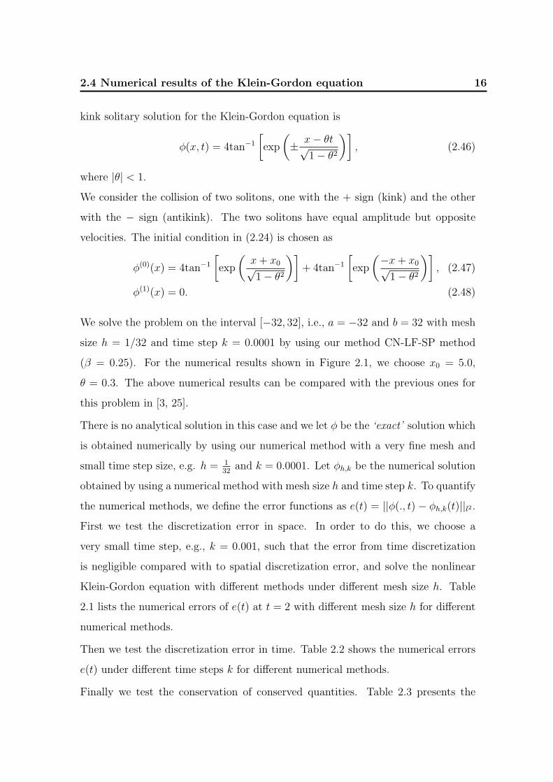
2.4 Numerical results of the Klein-Gordon equation 16
kink solitary solution for the Klein-Gordon equation is
φ(x, t) = 4tan−1
[exp
(± x− θt√
1− θ2
)], (2.46)
where |θ| < 1.
We consider the collision of two solitons, one with the + sign (kink) and the other
with the − sign (antikink). The two solitons have equal amplitude but opposite
velocities. The initial condition in (2.24) is chosen as
φ(0)(x) = 4tan−1
[exp
(x + x0√1− θ2
)]+ 4tan−1
[exp
(−x + x0√1− θ2
)], (2.47)
φ(1)(x) = 0. (2.48)
We solve the problem on the interval [−32, 32], i.e., a = −32 and b = 32 with mesh
size h = 1/32 and time step k = 0.0001 by using our method CN-LF-SP method
(β = 0.25). For the numerical results shown in Figure 2.1, we choose x0 = 5.0,
θ = 0.3. The above numerical results can be compared with the previous ones for
this problem in [3, 25].
There is no analytical solution in this case and we let φ be the ‘exact’ solution which
is obtained numerically by using our numerical method with a very fine mesh and
small time step size, e.g. h = 132
and k = 0.0001. Let φh,k be the numerical solution
obtained by using a numerical method with mesh size h and time step k. To quantify
the numerical methods, we define the error functions as e(t) = ||φ(., t)− φh,k(t)||l2 .First we test the discretization error in space. In order to do this, we choose a
very small time step, e.g., k = 0.001, such that the error from time discretization
is negligible compared with to spatial discretization error, and solve the nonlinear
Klein-Gordon equation with different methods under different mesh size h. Table
2.1 lists the numerical errors of e(t) at t = 2 with different mesh size h for different
numerical methods.
Then we test the discretization error in time. Table 2.2 shows the numerical errors
e(t) under different time steps k for different numerical methods.
Finally we test the conservation of conserved quantities. Table 2.3 presents the

2.4 Numerical results of the Klein-Gordon equation 17
a)
b)−30 −20 −10 0 10 20 300
5
10
15
20
25
30
35
40
45
50
x
t
Figure 2.1: Time evolution of soliton-soliton collision in Example 2.1. a): surface
plot; b): contour plot.
quantities at different times with mesh size h = 1/16 and time step k = 0.001 for
different numerical methods.
From Tables 2.1-2.3, we can draw the following observations: our numerical method
CN-LF-SP is of spectral-order accuracy in space discretization and second-order ac-
curacy in time. Finite difference methods (A, B and C) are of second-order accuracy
in space discretization. Moreover, CN-LF-SP with β = 1/2 or β = 1/4 are uncondi-
tionally stable, where CN-LF-SP with β = 0 is conditionally stable. However finite

2.4 Numerical results of the Klein-Gordon equation 18
Mesh h = 1.0 h = 1/2 h = 1/4
FDM A 0.131 4.659E-2 1.123E-2
FDM B 0.266 7.764E-2 1.986E-2
FDM C 0.173 5.608E-2 1.414E-2
CN-LF-SP (β = 0) 2.928E-2 5.037E-5 1.209E-7
CN-LF-SP (β = 1/4) 2.928E-2 5.033E-5 1.289E-7
CN-LF-SP (β = 1/2) 2.928E-2 5.030E-5 2.001E-7
Table 2.1: Spatial discretization errors e(t) at time t = 1 for different mesh sizes h
under k = 0.001.
Time Step k = 132
k = 164
k = 1128
k = 1256
k = 1512
CN-LF-SP(β = 0) - 9.057E-6 2.273E-6 5.843E-7 1.868E-7
CN-LF-SP(β = 1/4) 6.673E-5 1.668E-5 4.170E-6 1.044E-6 2.800E-7
CN-LF-SP(β = 1/2) 1.669E-4 4.173E-5 1.043E-5 2.606E-6 6.568E-7
Table 2.2: Temporal discretization errors e(t) at time t = 1 for different time steps
k under h = 1/16.
difference methods (A, B and C) are all conditionally stable in time. All of these
numerical methods conserve the energy H, the linear momentum P and angular
momentum A very well.
2.4.2 Applications of CN-LF-SP
Breather solution of the Klein-Gordon equation
Example 2.2 The nonlinear Klein-Gordon equation with a breather solution, i.e.,
we choose d = 1, F (φ) = sin(φ) in (1.1)-(1.2) and consider the problem on the
interval [a, b] with a = −40 and b = 40 with mesh size h = 5/256, time step
k = 0.001 and β = 0.25 for CN-LF-SP. The well-known breather solution is of the

2.4 Numerical results of the Klein-Gordon equation 19
Time H P A
FDM A 1.0 16.1640 0.0000 0.0000
2.0 16.1642 0.0000 0.0000
FDM B 1.0 16.1639 0.0000 0.0000
2.0 16.1639 0.0000 0.0000
FDM C 1.0 16.1641 0.0000 0.0000
2.0 16.1644 0.0000 0.0000
CN-LF-SP(β = 0) 1.0 16.1641 0.0000 0.0000
2.0 16.1644 0.0000 0.0000
CN-LF-SP(β = 1/4) 1.0 1.61641 0.0000 0.0000
2.0 16.1644 0.0000 0.0000
CN-LF-SP(β = 1/2) 1.0 1.61641 0.0000 0.0000
2.0 16.1644 0.0000 0.0000
Table 2.3: Conserved quantities analysis: k = 0.001 and h = 1/16.
form [49]
φ(x, t) = −4tan−1
[m√
1−m2
sin(t√
1−m2) + c2
cosh(mx + c1)
]. (2.49)
The initial condition is taken as φ(0)(x) = φ(x, 0), φ(1)(x) = φt(x, 0) in (2.49). In
the present example, we choose m = 0.5, c1 = 0, c2 = −10√
1−m2.
From the results shown in Figure 2.2, it is easy to see that they completely agree
with those presented in [25].
Ring solitary solution of the 2D Klein-Gordon equation
Example 2.3 The Klein-Gordon equation with a circular ring soliton solution in
2D case, i.e., we choose d = 2, F (φ) = sin(φ) in (1.1)-(1.2). The initial condition is

2.4 Numerical results of the Klein-Gordon equation 20
a)
b)−10 −5 0 5 10
0
5
10
15
20
25
30
x
t
Figure 2.2: Time evolution of a stationary Klein-Gordon’s breather solution in Ex-
ample 2.2. a): surface plot; b): contour plot.
taken as
φ(x, y, 0) = α tan−1[exp(3−
√x2 + y2)
], (2.50)
φt(x, y, 0) = 0, (x, y) ∈ R2, (2.51)
where α = 4.0 in our numerical simulation. We solve this problem on the rectangle
[−16, 16]2 with mesh size h = 1/16 and time step k = 0.001 by using our method
CN-LF-SP (β = 0.25). Figure 2.3 shows the surface plots of sin(φ/2) (left column)

2.4 Numerical results of the Klein-Gordon equation 21
and the contour plots of it (right column) at different times, i.e., t = 0, 4, 8, 11.5, 15.
The resolution is outstanding as compared with the existing numerical solutions
[4, 24]. It is found that the ring solitons shrink at the initial stage, but oscillations
and radiations begin to form and continue slowly as time goes on. This can be
clearly viewed in the contour plots.
Example 2.4 Two circular soliton-soliton collision in 2D of Klein Gordon equation,
i.e., we choose d = 2, F (φ) = sin(φ) in (1.1)-(1.2). The initial condition is taken as
φ(x, y, 0) = α tan−1{
exp[γ
(4−
√(x + 3)2 + (y + 7)2
)]}
+α tan−1{
exp[γ
(4−
√(x + 3)2 + (y + 17)2
)]}, (2.52)
φt(x, y, 0) = θ sech[γ
(4−
√(x + 3)2 + (y + 7)2
)]
+θ sech[γ
(4−
√(x + 3)2 + (y + 17)2
)], (x, y) ∈ R2,(2.53)
where α = 4.0, θ = 4.13, γ = 2.29 in our simulation. We solve this problem on the
rectangle [−30, 10] × [−27, 13] with mesh size h = 1/16 and time step k = 0.001
by using our method CN-LF-SP (β = 0.25). Numerical simulation presented in
Figure 2.4 is for sin(φ/2) at time t = 0, 2, 4, 6, 8, respectively. The solution shown
includes the extension across x = −10 and y = −7 by symmetry properties of the
problem [24]. Figure 2.4 demonstrates the collision between two expanding circular
ring solitons in which two smaller ring solitons bounding an annular region merge
into a large ring soliton. The simulated solution is again precisely consistent to
existing results [24]. Contour plots are given to show more clearly the movement
of solitons. Though minor disturbances can be observed in the middle of the nu-
merical solution, probably due to the transactions following the symmetry features
in computations, the overall simulation results match well with those described in
[19, 24] with satisfaction.
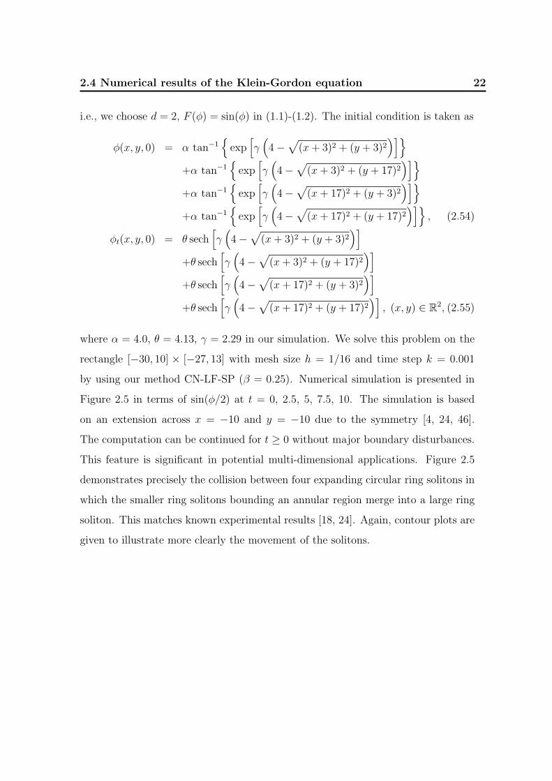
Example 2.5 The collision of four circular solitons in 2D of Klein Gordon equation,
2.4 Numerical results of the Klein-Gordon equation 22
i.e., we choose d = 2, F (φ) = sin(φ) in (1.1)-(1.2). The initial condition is taken as
φ(x, y, 0) = α tan−1{
exp[γ
(4−
√(x + 3)2 + (y + 3)2
)]}
+α tan−1{
exp[γ
(4−
√(x + 3)2 + (y + 17)2
)]}
+α tan−1{
exp[γ
(4−
√(x + 17)2 + (y + 3)2
)]}
+α tan−1{
exp[γ
(4−
√(x + 17)2 + (y + 17)2
)]}, (2.54)
φt(x, y, 0) = θ sech[γ
(4−
√(x + 3)2 + (y + 3)2
)]
+θ sech[γ
(4−
√(x + 3)2 + (y + 17)2
)]
+θ sech[γ
(4−
√(x + 17)2 + (y + 3)2
)]
+θ sech[γ
(4−
√(x + 17)2 + (y + 17)2
)], (x, y) ∈ R2, (2.55)
where α = 4.0, θ = 4.13, γ = 2.29 in our simulation. We solve this problem on the
rectangle [−30, 10] × [−27, 13] with mesh size h = 1/16 and time step k = 0.001
by using our method CN-LF-SP (β = 0.25). Numerical simulation is presented in
Figure 2.5 in terms of sin(φ/2) at t = 0, 2.5, 5, 7.5, 10. The simulation is based
on an extension across x = −10 and y = −10 due to the symmetry [4, 24, 46].
The computation can be continued for t ≥ 0 without major boundary disturbances.
This feature is significant in potential multi-dimensional applications. Figure 2.5
demonstrates precisely the collision between four expanding circular ring solitons in
which the smaller ring solitons bounding an annular region merge into a large ring
soliton. This matches known experimental results [18, 24]. Again, contour plots are
given to illustrate more clearly the movement of the solitons.

2.4 Numerical results of the Klein-Gordon equation 23
−15 −10 −5 0 5 10 15
−15
−10
−5
0
5
10
15
x
y
−15 −10 −5 0 5 10 15
−15
−10
−5
0
5
10
15
x
y
−15 −10 −5 0 5 10 15
−15
−10
−5
0
5
10
15
x
y
−15 −10 −5 0 5 10 15
−15
−10
−5
0
5
10
15
x
y
−15 −10 −5 0 5 10 15
−15
−10
−5
0
5
10
15
x
y
Figure 2.3: Circular and elliptic ring solitons in Example 2.3 (from top to bottom:
t = 0, 4, 8, 11.5 and 15).

2.4 Numerical results of the Klein-Gordon equation 24
−20 −10 0 10−30
−25
−20
−15
−10
−5
0
5
x
y
−20 −10 0 10−30
−25
−20
−15
−10
−5
0
5
x
y
−20 −10 0 10−30
−25
−20
−15
−10
−5
0
5
x
y
−20 −10 0 10−30
−25
−20
−15
−10
−5
0
5
x
y
−20 −10 0 10−30
−25
−20
−15
−10
−5
0
5
x
y
Figure 2.4: Collision of two ring solitons in Example 2.4 (from top to bottom : t = 0,
2, 4, 6 and 8).

2.4 Numerical results of the Klein-Gordon equation 25
−30 −20 −10 0−30
−25
−20
−15
−10
−5
0
5
x
y
−30 −20 −10 0−30
−25
−20
−15
−10
−5
0
5
x
y
−30 −20 −10 0−30
−25
−20
−15
−10
−5
0
5
x
y
−30 −20 −10 0−30
−25
−20
−15
−10
−5
0
5
x
y
−30 −20 −10 0−30
−25
−20
−15
−10
−5
0
5
x
y
Figure 2.5: Collision of four ring solitons in Example 2.5 (from top to bottom: t = 0,
2.5, 5, 7.5 and 10).

Chapter 3The Klein-Gordon-Schrodinger equations
In this chapter, the Klein-Gordon-Schrodinger equations describing a system of con-
served scalar nucleons interacting with neutral scalar mesons, are derived and its
analytical properties are analyzed.
3.1 Derivation of the Klein-Gordon-Schrodinger
equations
This section is devoted to derive the Klein-Gordon-Schrodinger equations. The
Lagrangian density of the dynamic system that describes the interaction between
the complex scalar nucleon field and real scalar meson field in one dimension (1D)
is
L = Lo + Lint
= i ~ψ∗ψt +~2
2mψ∗ψxx +
1
2(φ2
t − φ2x − µ2φ2) + g2φ|ψ|2, (3.1)
where ψ represents the complex scalar nucleon field, φ describes the real scalar me-
son field, g2φ|ψ|2 is the Yukawa interaction potential, and m, µ respectively describe
the mass of nucleon and mass of meson.
26

3.1 Derivation of the Klein-Gordon-Schrodinger equations 27
Since the Lagrangian of the whole system must satisfy the Euler-Lagrange equation
(that is, ∂∂ct
∂L∂( ∂η
∂ct)+ ∂
∂x∂L
∂( ∂η∂x
)− ∂L
∂η= 0). Then we can get the equations of motion of
the whole system.
Let η = ψ∗, we get the equation
i~ψt +~2
2mψxx + g2ψφ = 0. (3.2)
Let η = φ,we get another equation
¤φ + µ2φ− g2|ψ|2 = 0, (3.3)
where ¤ = 1c2
∂2
∂t2− ∂xx.
In general, we can obtain the equations of motion of the dynamic system in d-
dimension (d = 1, 2, 3).
i~ψt +~2
2m∇2ψ + g2ψφ = 0, (3.4)
¤φ + µ2φ− g2|ψ|2 = 0, (3.5)
where ¤ = 1c2
∂2
∂t2− ∇2. In order to obtain a dimensionless form of the KGS (3.4)-
(3.5), we define the normalized variables
t =~µ2
2mt, x = µx, (3.6)
ψ =g2√
2m
~µ2ψ, φ =
2mg2
~2µ2φ. (3.7)
Then defining
ε =~µ
2mc, (3.8)
and plugging (3.6)-(3.7) into (3.4)-(3.5), and then removing all ‘∼’, we get the
following dimensionless standard Klein-Gordon-Schrodinger equations
i ∂tψ + ∆ψ + φψ = 0, (3.9)
ε2∂ttφ−∆φ + φ− |ψ|2 = 0. (3.10)

3.2 Conservation laws of the Klein-Gordon-Schrodinger equations 28
Adding dissipative terms to (3.9), we can obtain the generalized Klein-Gordon-
Schrodinger equations
i ∂tψ + ∆ψ + φψ + iνψ = 0, (3.11)
ε2∂ttφ + γε∂tφ−∆φ + φ− |ψ|2 = 0. (3.12)
3.2 Conservation laws of the Klein-Gordon-Schrodinger
equations
Define the wave energy
D(t) := D(ψ(·, t)) =
∫
Rd
|ψ(x, t)|2 dx, t ≥ 0, (3.13)
and the Hamiltonian
H(t) =
∫
Rd
[1
2
(φ2(x, t) + ε2(∂tφ(x, t))2 + |∇φ(x, t)|2) + |∇ψ(x, t)|2
−|ψ(x, t)|2φ(x, t)]dx, t ≥ 0. (3.14)
Lemma 3.1. Suppose (ψ, φ) be the solution of the generalized Klein-Gordon-Schrodinger
equations (1.4)-(1.5), its wave energy and Hamiltonian has the following properties
d
dtD(t) =
d
dt
∫
Rd
|ψ(x, t)|2 dx = −2ν
∫
Rd
|ψ(x, t)|2 dx, t ≥ 0, (3.15)
d
dtH(t) =
d
dt
∫
Rd
[1
2
(φ2(x, t) + ε2(∂tφ(x, t))2 + |∇φ(x, t)|2) + |∇ψ(x, t)|2
−|ψ(x, t)|2φ(x, t)]dx
= −∫
Rd
[γε(∂tφ(x, t))2 + iν (∂tψ
∗(x, t)ψ(x, t)
−∂tψ(x, t)ψ∗(x, t))] dx, t ≥ 0. (3.16)
Proof. Multiplying (1.4) by ψ∗, the conjugate of ψ, we get
i ψtψ∗ + ∆ψψ∗ + φ|ψ|2 + i ν|ψ|2 = 0. (3.17)
Then taking the conjugate of (1.5) and multiplying it by ψ, we obtain
−i ψ∗t ψ + ψ∆ψ∗ + φ|ψ|2 − i ν|ψ|2 = 0. (3.18)

3.2 Conservation laws of the Klein-Gordon-Schrodinger equations 29
Subtracting (3.18) from (3.17) and then multiplying both sides by −i, we can get
ψtψ∗ + ψ∗t ψ + i (ψ∆ψ∗ − ψ∗∆ψ) + 2ν|ψ|2 = 0. (3.19)
Integrating over Rd, integration by parts, (3.19) leads to
d
dtD(t) =
d
dt
∫
Rd
|ψ(x, t)|2 dx = −2ν
∫
Rd
|ψ(x, t)|2 dx, t ≥ 0, (3.20)
which implies that D(t) preserves as a constant when ν = 0.
Multiplying (1.4) by ψ∗t , we get
i |ψt|2 + ∆ψψ∗t + φψψ∗t + i νψψ∗t = 0. (3.21)
Then taking the conjugate of (1.5) and multiplying it by ψt, we obtain
−i |ψt|2 + ψt∆ψ∗ + φψ∗ψt − i νψ∗ψt = 0. (3.22)
Adding (3.21) to (3.22), we can get
(ψ∆ψ∗t + ψt∆ψ∗) + φ(|ψ|2)t + i ν(ψψ∗t − ψ∗ψt) = 0 (3.23)
Integrating over Rd (3.19) leads to
∫
Rd
[(ψ∆ψ∗t + ψt∆ψ∗) + φ(|ψ|2)t + i ν(ψψ∗t − ψ∗ψt)
]dx = 0. (3.24)
Multiplying (1.5) by φt, and integrating over Rd, we can get
∫
Rd
[ε2φttφt + γε(φt)
2 −∆φφt + φφt − |ψ|2φt
]dx = 0 (3.25)
Noting (3.25), (3.24) and (3.20), we obtain
d
dtH(t) =
∫
Rd
[φφt + ε2φtφtt +∇φ · ∇φt + (|∇ψ|2 − |ψ|2φ)t
]dx
=
∫
Rd
[−γε(φt)2 + ∆φφt + |ψ|2φt +∇φ · ∇φt + (|∇ψ|2 − |ψ|2φ)t
]dx
=
∫
Rd
[∆φφt +∇φ · ∇φt] dx +
∫
Rd
[−(|ψ|2)tφ + (|∇ψ|2)t
]dx−
∫
Rd
γε(φt)2dx
= −∫
Rd
[γε(φt)
2 + i ν (ψtψ∗ − ψ∗t ψ)
]dx, t ≥ 0, (3.26)
3.3 Dynamics of mean value of the meson field 30
which implies that H(t) is decreasing if ν = 0 as time t is increasing and H(t)
preserves as a constant when ν = 0 and γ = 0. ¤From the above discussion, we find that when γ = 0 and ν = 0 in (1.4)-(1.5), the
KGS has at least two invariants.
Theorem 3.1. The generalized Klein-Gordon-Schrodinger equations (1.4)-(1.5) with
γ = ν = 0 preserve the conserved quantities. They are the wave energy
D(t) := D(ψ(·, t)) =
∫
Rd
|ψ(x, t)|2 dx ≡∫
Rd
|ψ(0)(x)|2 dx := D(0), t ≥ 0,
(3.27)
and the Hamiltonian
H(t) =
∫
Rd
[1
2
(φ2(x, t) + ε2(∂tφ(x, t))2 + |∇φ(x, t)|2) + |∇ψ(x, t)|2
−|ψ(x, t)|2φ(x, t)]dx
≡∫
Rd
[1
2
((φ(0)(x))2 + ε2(φ(1)(x))2 + |∇φ(0)(x)|2) + |∇ψ(0)(x)|2
−|ψ(0)(x)|2φ(0)(x)]dx
:= H(0), t ≥ 0. (3.28)
In one dimension case, the conserved quantities become
H =
∫ ∞
−∞
[1
2
(φ2(x, t) + ε2 (φt(x, t))2 + (φx(x, t))2) + |ψ(x, t)|2
−|ψ(x, t)|2φ(x, t)
]dx, (3.29)
A =
∫ ∞
−∞|ψ(x, t)|2 dx. (3.30)
3.3 Dynamics of mean value of the meson field
When ν = 0, the generalized KGS (1.4)-(1.5) collapses to
i ∂tψ + ∆ψ + φψ = 0, x ∈ Rd, t > 0, (3.31)
ε2∂ttψ + γε∂tφ−∆φ + φ− |ψ|2 = 0, x ∈ Rd, t > 0. (3.32)

3.4 Plane wave and soliton wave solutions of KGS 31
Define the mean value of the meson field as
N(t) := N(φ(·, t)) =
∫
Rd
φ(x, t) dx, t ≥ 0. (3.33)
Integrating (3.32) over Rd, integration by parts and noticing (3.27), we obtain
ε2N ′′(t) + γεN ′(t) + N(t) = D(0), t ≥ 0, (3.34)
with initial condition as
N(0) = N(φ(0)) :=
∫
Rd
φ(0)(x) dx, N ′(0) = N(φ(1)) :=
∫
Rd
φ(1)(x) dx. (3.35)
Denote
λ01 =
−γ +√
γ2 − 4
2ε, λ0
2 =−γ −
√γ2 − 4
2ε, λ0 =
−γ
2ε, β0 =
√4− γ2
2ε. (3.36)
Solving the ODE (3.34) with the initial data (3.35), we get the dynamics of the
mean value of the meson field when ν = 0:
(i) For γ > 2
N(t) = D(0)+N(φ(1))− λ0
2(N(φ(0))−D(0))
λ01 − λ0
2
eλ01t+
−N(φ(1)) + λ01(N(φ(0))−D(0))
λ01 − λ0
2
eλ02t;
(ii) for γ = 2
N(t) = D(0) +(N(φ(0))−D(0)
)eλ0t +
(N(φ(1) − λ0(N(φ(0))−D(0))
)teλ0t;
and (iii) for 0 ≤ γ < 2
N(t) = D(0)+eλ0t
[(N(φ(0))−D(0)
)cos(β0t) +
N(φ(1))− λ0(N(φ(0))−D(0))
β0
sin(β0t)
].
These immediately imply that limt→∞ N(t) = D(0) when γ > 0, and N(t) is a
periodic function with period T = 2επ when γ = 0.
3.4 Plane wave and soliton wave solutions of KGS
When d = 1, γ = 0, ν = 0, and ε = 1, the generalized KGS (1.4)-(1.5) collapses to
i ∂tψ + ∆ψ + φψ = 0, x ∈ R, t > 0, (3.37)
∂ttφ−∆φ + φ− |ψ|2 = 0, x ∈ R, t > 0, (3.38)

3.5 Reduction to the Schrodinger-Yukawa equations (S-Y) 32
which admits plane and soliton wave solutions.
Firstly, it is instructive to examine some explicit solutions to (3.37) and (3.38). The
initial data in (1.6) is chosen as
φ(0)(x) = d > 0, φ(1)(x) = 0, ψ(0)(x) =√
d exp
(i2πlx
b− a
), x ∈ R, (3.39)
with l an integer, and a, b and d constants, the KGS admits the plane wave solution
[22].
φ(x, t) = d, ψ(x, t) =√
d exp
[i
(2πlx
b− a− ωt
)], x ∈ R, t ≥ 0, (3.40)
where
ω =
(2πl
b− a
)2
− d.
Secondly, as it is well known, the standard KGS is not completely integrable. There-
fore the generalized KGS can not be exactly integrable either. However, it has
one-soliton solutions to (3.37) and (3.38) for d = 1, γ = 0, ν = 0 [38]
ψ±(x, t) = 3B sech2 (Bx + c±t) exp[i(d±x +
(4B2 − d2
±)t)]
, (3.41)
φ±(x, t) = 6B2 sech2 (Bx + c±t) , x ∈ R, t ≥ 0, (3.42)
where
c± = ±√
4B2 − 1
2ε, d± = ∓
√4B2 − 1
4B= − c±
2B,
with B ≥ 1/2 a constant.
Note that the phase in ψ oscillates as O(1ε). This exact solution is used in Chapter
4 to test the accuracy of our new numerical methods.
3.5 Reduction to the Schrodinger-Yukawa equa-
tions (S-Y)
In the ”nonrelativistic regime”, i.e., ε → 0 in (1.4)-(1.6), which corresponds to
infinite speed of light, we can obtain the well-known Schrodinger-Yukawa equations

3.5 Reduction to the Schrodinger-Yukawa equations (S-Y) 33
without (ν = 0) or with (ν > 0) a linear damping term:
i ∂tψ + ∆ψ + φψ + i νψ = 0, x ∈ Rd, t > 0, (3.43)
−∆φ + φ = |ψ|2, x ∈ Rd, t > 0. (3.44)
When ν = 0, the S-Y equations (1.7)-(1.8) is time reversible, time transverse invari-
ant, and preserves the following wave energy and Hamiltonian:
DSY =
∫
Rd
|ψ(x, t)|2 dx, (3.45)
HSY =
∫
Rd
[1
2
(φ2(x, t) + |∇φ(x, t)|2) + |∇ψ(x, t)|2 − |ψ(x, t)|2φ(x, t)
]dx.(3.46)
Similarly, letting ε → 0 in (3.28), we get formally the quadratic convergence rate
of the Hamiltonian from KGS with ν = γ = 0 to S-Y in the “nonrelativistic” limit
regime, i.e., 0 < ε ¿ 1:
H(t) =
∫
Rd
[1
2
(φ2(x, t) + |∇φ(x, t)|2) + |∇ψ(x, t)|2 − |ψ(x, t)|2φ(x, t)
]dx
+ε2
∫
Rd
(∂tφ(x, t))2 dx
≈ HSY + O(ε2). (3.47)
Our numerical results in Chapter 5 confirm this asymptotic result.

Chapter 4Numerical studies of the
Klein-Gordon-Schrodinger equations
In this Chapter, we present two accurate and efficient numerical schemes, phase
space analytical solver+time-splitting spectral method (PSAS-TSSP) and Crank-
Nicolson leap-frog time-splitting spectral method (CN-LF-TSSP) for the Klein-
Gordon-Schrodinger equations (1.4)-(1.5) with the periodic boundary conditions
and analyze the numerical properties for these two numerical methods. Then we
compare the accuracy and stability of different numerical methods for the Klein-
Gordon-Schrodinger equations with a solitary wave solution, and also present the
numerical results for plane waves, soliton-soliton collisions in 1D, 2D problems and
the generalized KGS with a damping term.
4.1 Numerical methods for the Klein-Gordon-Schrodinger
equations
In this section we present two new accurate and efficient numerical methods, i.e.,
phase space analytical+time-splitting spectral discretizations (PSAS-TSSP) and
34

4.1 Numerical methods for the Klein-Gordon-Schrodinger equations 35
Crank-Nicolson leap-frog spectral discretization (CN-LF-TSSP) for the Klein-Gordon-
Schrodinger equations (1.4)-(1.6) with the periodic boundary conditions.
For simplicity of notation, we shall introduce the method in 1D of the KGS with
periodic boundary conditions. Generalizations to higher dimensions are straightfor-
ward for tensor product grids and the results remain valid without modifications.
For d = 1, the problem becomes
i ∂tψ(x, t) + ∂xxψ + iνψ + φψ = 0, a < x < b, t > 0, (4.1)
ε2∂ttφ + εγ∂tφ− ∂xxφ + φ− |ψ|2 = 0, a < x < b, t > 0, (4.2)
ψ(a, t) = ψ(b, t), ∂xψ(a, t) = ∂xψ(b, t), t ≥ 0, (4.3)
φ(a, t) = φ(b, t), ∂xφ(a, t) = ∂xφ(b, t), t ≥ 0, (4.4)
ψ(x, 0) = ψ(0)(x), φ(x, 0) = φ(0)(x), ∂tφ(x, 0) = φ(1)(x), a ≤ x ≤ b. (4.5)
As it is well known, the above KGS in 1D has the following properties:
D(t) =
∫ b
a
|ψ(x, t)|2dx = e−2νt
∫ b
a
|ψ(0)(x)|2dx = e−2νtD(0), t ≥ 0. (4.6)
So when ν = 0, D(t) ≡ D(0), i.e., it is an invariant of the KGS. When ν > 0,
it decays to 0 exponentially. Furthermore, when ν = 0 and γ = 0, the KGS also
conserves the Hamiltonian:
H(t) =
∫ a
b
[1
2
(φ(x, t)2 + ε2(∂tφ(x, t))2 + (∂xφ(x, t))2
)+ |∂xψ(x, t)|2
−|ψ(x, t)|2φ(x, t)]dx ≡ H(0), t ≥ 0. (4.7)
In some cases, the periodic boundary conditions (4.3) and (4.4) may be replaced by
the homogeneous Dirichlet boundary conditions
ψ(a, t) = ψ(b, t) = 0, φ(a, t) = φ(b, t) = 0, t ≥ 0. (4.8)
We choose the spatial mesh size h = ∆x > 0 with h = (b − a)/M for M being an
even positive integer, the time step size being k = ∆t > 0 and let the grid points
and the time step be
xj := a + jh, j = 0, 1, · · · ,M ; tm := mk, m = 0, 1, 2, · · · .

4.1 Numerical methods for the Klein-Gordon-Schrodinger equations 36
Let ψmj and φm
j be the approximations of ψ(xj, tm) and φ(xj, tm), respectively. Fur-
thermore, let ψm and φm be the solution vector at time t = tm = mk with compo-
nents ψmj and φm
j , respectively.
4.1.1 Time-splitting for the nonlinear Schrodinger equation
From time t = tm and t = tm+1, the first NLS-type equation (4.1) is solved in two
splitting steps [5, 6, 8, 9, 63]. One solves first
i∂tψ + ∂xxψ = 0, (4.9)
for the time step of length k, followed by solving
i∂tψ + iνψ + φψ = 0, (4.10)
for the same time step. Equation (4.9) will be discretized in space by the Fourier
spectral method and integrated in time exactly. For each fixed x ∈ [a, b], integrating
(4.10) from time t = tm to t = tm+1 = tm + k, and then approximating the integral
on [tm, tm+1] via the trapezoidal rule [11, 12, 10], we obtain
ψ(x, tm+1) = exp
[∫ tm+1
tm
(−ν + iφ(x, τ)) dτ
]ψ(x, tm)
= exp
[−νk + ik
φ(x, tm) + φ(x, tm+1)
2
]ψ(x, tm), a ≤ x ≤ b. (4.11)
4.1.2 Phase space analytical solver+time-splitting spectral
discretizations (PSAS-TSSP)
The Klein-Gordon equation (4.2) in KGS is discretized by using a pseudospectral
method for spatial derivatives and then solving the ODEs in phase space analytically
under appropriate chosen transmission conditions between different time intervals.
From time t = tm to t = tm+1, assume
φ(x, t) =
M/2−1∑
l=−M/2
φml (t)eiµl(x−a), a ≤ x ≤ b, tm ≤ t ≤ tm+1, (4.12)

4.1 Numerical methods for the Klein-Gordon-Schrodinger equations 37
where µl = 2πlb−a
and φml (t) is the Fourier coefficient of lth mode. Plugging (4.12) into
(4.2) and noticing the orthogonality of the Fourier functions, we get the following
ODEs for m ≥ 0 and tm ≤ t ≤ tm+1:
ε2d2φml (t)
dt2+ εγ
dφml (t)
dt+ (µ2
l + 1)φml (t)− ˜(|ψ(tm)|2)l = 0, (4.13)
φml (tm) =
(φ(0))l, m = 0,
φm−1l (tm), m > 0,
l = −M
2, ...,
M
2− 1. (4.14)
For each fixed l (−M/2 ≤ l ≤ M/2− 1), equation (4.13) is a second-order ODE. It
needs two initial conditions such that the solution is unique. When m = 0 in (4.13)
and (4.14), we have the initial condition (4.14) and we can pose the other initial
condition for (4.13) due to the initial condition (4.5):
d
dtφ0
l (t0) =d
dtφ0
l (0) = (φ(1))l, l = −M
2, ...,
M
2− 1. (4.15)
Denote
λ1 =−γ +
√γ2 − 4(µ2
l + 1)
2ε, λ2 =
−γ −√
γ2 − 4(µ2l + 1)
2ε, β =
√4(µ2
l + 1)− γ2
2ε.
(4.16)
Then the solution of (4.13), (4.14) with m = 0 and (4.15) for l (−M/2 ≤ l < M/2)
and 0 ≤ t ≤ t1 is:
(i) For γ2 − 4(µ2l + 1) > 0
φ0l (t) =
˜(|ψ(0)|2)l
µ2l + 1
+ε√
γ2 − 4(µ2l + 1)
[(φ(1))l −
((φ(0))l −
˜(|ψ(0)|2)l
µ2l + 1
)λ2
]eλ1t
− ε√γ2 − 4(µ2
l + 1)
[(φ(1))l −
((φ(0))l −
˜(|ψ(0)|2)l
µ2l + 1
)λ1
]eλ2t; (4.17)
(ii) for γ2 − 4(µ2l + 1) = 0,
φ0l (t) =
˜(|ψ(0)|2)l
µ2l + 1
+
[(φ(0))l −
˜(|ψ(0)|2)l
µ2l + 1
+
((φ(1))l +
γ
2ε
((φ(0))l −
˜(|ψ(0)|2)l
µ2l + 1
))t
]e−
γt2ε ;
(4.18)

4.1 Numerical methods for the Klein-Gordon-Schrodinger equations 38
and (iii) for γ2 − 4(µ2l + 1) < 0
φ0l (t) = e−
γt2ε
[1
β
((φ(1))l +
γ
2ε((φ(0))l −
˜(|ψ(0)|2)l
µ2l + 1
)
)sin(βt)
+
((φ(0))l −
˜(|ψ(0)|2)l
µ2l + 1
)cos(βt)
]+
˜(|ψ(0)|2)l
µ2l + 1
. (4.19)
But when m > 0, we only have one initial condition (4.14). One can’t simply pose
the continuity between ddt
φml (t) and d
dtφm−1
l (t) across the time t = tm, because the
last term in (4.13) is usually different in two adjacent time intervals [tm−1, tm] and
[tm, tm+1]; i.e., ˜(|ψ(tm−1)|2)l 6= ˜(|ψ(tm)|2)l. Since our goal is to develop an explicit
scheme and we need to linearize the nonlinear term in (4.2) in our discretization
(4.13), in general,
d
dtφm−1
l (t−m) = limt→t−m
d
dtφm−1
l (t) 6= limt→t+m
d
dtφm
l (t) =d
dtφm
l (t+m),
m = 1, 2, ..., l = −M
2, ...,
M
2− 1. (4.20)
Unfortunately, we don’t know the jump ddt
φml (t+m) − d
dtφm−1
l (t−m) across the time
t = tm. In order to get a unique solution of (4.13) and (4.14) for m > 0, we pose
here an additional condition:
φml (tm−1) = φm−1
l (tm−1), l = −M
2, ...,
M
2− 1. (4.21)
The condition (4.21) is equivalent to posing that the solution φml (t) on the time
interval [tm, tm+1] of (4.13)-(4.14) is also continuous at the time t = tm−1. After a
simple computation, we get the solution of (4.13), (4.14) and (4.21) with m > 0 for
l (l = −M/2, ..., M/2− 1) and tm ≤ t ≤ tm+1:
(i) For γ2 − 4(µ2l + 1) > 0
φml (t) =
1
e−kλ1 − e−kλ2
[˜(|ψm|2)l
µ2l + 1
(e−kλ2 − 1) + φm−1l (tm−1)− φm−1
l (tm)e−kλ2
]eλ1(t−tm)
+1
e−kλ2 − e−kλ1
[˜(|ψm|2)l
µ2l + 1
(e−kλ1 − 1) + φm−1l (tm−1)− φm−1
l (tm)e−kλ1
]eλ2(t−tm)
+˜(|ψm|2)l
µ2l + 1
; (4.22)

4.1 Numerical methods for the Klein-Gordon-Schrodinger equations 39
(ii) for γ2 − 4(µ2l + 1) = 0
φml (t) =
[t− tm
k
(φm−1
l (tm)−˜(|ψm|2)l
µ2l + 1
+ e−kγ2ε
(˜(|ψm|2)l
µ2l + 1
− φm−1l (tm−1)
))
+φm−1l (tm)−
˜(|ψm|2)l
µ2l + 1
]e−
γ(t−tm)2ε +
˜(|ψm|2)l
µ2l + 1
; (4.23)
and (iii) for γ2 − 4(µ2l + 1) < 0
φml (t) = e−
γ(t−tm)2ε
[(φm−1
l (tm)−˜(|ψm|2)l
µ2l + 1
)(cos(β(t− tm)) + cot(βk) sin(β(t− tm)))
+e−γk2ε
(˜(|ψm|2)l
µ2l + 1
− φm−1l (tm−1)
)sin(β(t− tm))
sin(βk)
]+˜(|ψm|2)l
µ2l + 1
. (4.24)
From time t = tm to t = tm+1, we combine the splitting steps via the standard
Strang splitting [61, 5, 8]:
φm+1j =
M/2−1∑
l=−M/2
(φm+1)l eiµl(xj−a), (4.25)
ψ∗j =
M/2−1∑
l=−M/2
e−ikµ2l /2(ψm)l eiµl(xj−a),
ψ∗∗j = e−νk+ik(φmj +φm+1
j )/2 ψ∗j ,
ψm+1j =
M/2−1∑
l=−M/2
e−ikµ2l /2(ψ∗∗)l eiµl(xj−a), 0 ≤ j ≤ M − 1, m ≥ 0; (4.26)
where Ul, the Fourier coefficients of a vector U = (U0, U1, U2, · · · , UM)T with U0 =
UM , are defined as
Ul =1
M
M−1∑j=0
Uje−iµl(xj−a), l = −M
2, · · · ,
M
2− 1, (4.27)
and (i) for γ2 − 4(µ2l + 1) > 0
(φm+1)l =
ε(eλ1k−eλ2k)√γ2−4(µ2
l +1)(φ(1))l + ε(λ1eλ2k−λ2eλ1k)√
γ2−4(µ2l +1)
(φ(0))l m = 0
+
(ε(λ2eλ1k−λ1eλ2k)√
γ2−4(µ2l +1)
+ 1
)˜(|ψ(0)|2)l
µ2l +1
,
−e(λ1+λ2)k (φm−1)l + (eλ1k + eλ2k)(φm)l m ≥ 1
+(eλ1k − 1
) (eλ2k − 1
) ˜(|ψm|2)l
µ2l +1
;
(4.28)

4.1 Numerical methods for the Klein-Gordon-Schrodinger equations 40
(ii) for γ2 − 4(µ2l + 1) = 0
(φm+1)l =
(1 + γk2ε
)e−γk2ε (φ(0))l + ke−
γk2ε (φ(1))l m = 0
−((1 + γk
2ε)e−
γk2ε − 1
) ˜(|ψ(0)|2)l
µ2l +1
,
2e−kγ2ε (φm)l − e−
γkε (φm−1)l m ≥ 1
+(e−
γk2ε − 1
)2 ˜(|ψm|2)l
µ2l +1
;
(4.29)
and (iii) for γ2 − 4(µ2l + 1) < 0
(φm+1)l =
(cos(βk) + γ2βε
sin(βk))e−γk2ε (φ(0))l + sin(βk)
βe−
γk2ε (φ(1))l m = 0
−((cos(βk) + γ
2βεsin(βk))e−
γk2ε − 1
) ˜(|ψ(0)|2)l
µ2l +1
,
−e−γkε (φm−1)l + 2 cos(βk)e−
γk2ε (φm)l m ≥ 1
−(2 cos(βk)e−
γk2ε − e−
γkε − 1
) ˜(|ψm|2)l
µ2l +1
.
(4.30)
The initial conditions (4.5) are discretized as
ψ0j = ψ(0)(xj), φ0
j = φ(0)(xj), φ(1)j = φ(1)(xj), 0 ≤ j ≤ M. (4.31)
Note that the spatial discretization error of the above method is of spectral order
accuracy in h, and the time discretization error is demonstrated to be of second
order accuracy in k in section 4.3.1 from our numerical results.
4.1.3 Crank-Nicolson leap-frog time-splitting spectral dis-
cretizations (CN-LF-TSSP)
Another way to discretize the Klein-Gordon equation (4.2) in the KGS is by using
a pseudospectral method for spatial derivatives, followed by application of a Crank-
Nicolson/leap-frog method for linear/nonlinear terms for time derivatives:
ε2φm+1
j − 2φmj + φm−1
j
k2+ εγ
φm+1j − φm−1
j
2k−Df
xx
(βφm+1 + (1− 2β)φm + βφm−1)
)x=xj
+(βφm+1
j + (1− 2β)φmj + βφm−1
j
)− |ψmj |2 = 0, 0 ≤ j ≤ M, m ≥ 0, (4.32)

4.1 Numerical methods for the Klein-Gordon-Schrodinger equations 41
where 0 ≤ β ≤ 1/2 is a constant; Dfxx, a spectral differential operator approximation
of ∂xx, is defined as
DfxxU |x=xj
= −M/2−1∑
l=−M/2
µ2l Ul eiµl(xj−a). (4.33)
When β = 0 in (4.32), the discretization (4.32) to the equation (4.2) is explicit.
When 0 < β ≤ 1/2, the discretization is implicit, but can be solved explicitly. In
fact, suppose
φmj =
M/2−1∑
l=−M/2
(φm)leiµl(xj−a), j = 0, · · · ,M, m = 0, 1, .... (4.34)
Plugging (4.34) into (4.32) and using the orthogonality of the Fourier functions, we
obtain for m ≥ 1
ε2 (φm+1)l − 2(φm)l + (φm−1)l
k2+ εγ
(φm+1)l − (φm−1)l
2k− ˜(|ψm|2)l
+(µ2l + 1)
(β(φm+1)l + (1− 2β)(φm)l + β(φm−1)l
)= 0, 0 ≤ j ≤ M.(4.35)
Solving the above equation, we get
(φm+1)l =4ε2 + 2(2β − 1)(µ2
l + 1)k2
2k2β(µ2l + 1) + εγk + 2ε2
(φm)l −(
1− 2εγk
2k2β(µ2l + 1) + εγk + 2ε2
)(φm−1)l
+2k2
2k2β(µ2l + 1) + εγk + 2ε2
˜(|ψm|2)l, −M
2≤ l <
M
2, m ≥ 1. (4.36)
From time t = tm to t = tm+1, we combine the splitting steps via the standard
Strang splitting [61, 5, 8]:
φm+1j =
M/2−1∑
l=−M/2
(φm+1)l eiµl(xj−a), (4.37)
ψ∗j =
M/2−1∑
l=−M/2
e−ikµ2l /2 (ψm)l eiµl(xj−a),
ψ∗∗j = e−νk+ik(φmj +φm+1
j )/2 ψ∗j
ψm+1j =
M/2−1∑
l=−M/2
e−ikµ2l /2 (ψ∗∗)l eiµl(xj−a), 0 ≤ j ≤ M − 1, m ≥ 0. (4.38)
4.2 Properties of numerical methods 42
The initial conditions are discretized as
ψ0j = ψ(0)(xj), φ0
j = φ(0)(xj),φ1
j − φ−1j
2k= φ(1)(xj), 0 ≤ j ≤ M − 1. (4.39)
This implies that
(φ1)l =2ε2 + (2β − 1)(µ2
l + 1)k2
2 (ε2 + β(µ2l + 1)k2)
(φ(0))l +k (2k2β(µ2
l + 1)− εγk + 2ε2)
2 (ε2 + β(µ2l + 1)k2)
(φ(1))l
+k2
2 (ε2 + β(µ2l + 1)k2)
˜(|ψ(0)|2)l. (4.40)
Note that the spatial discretization error of the method is of spectral order accuracy
in h and the time discretization error is demonstrated to be second order accurate
in k in section 4.3.1 from our numerical results.
4.2 Properties of numerical methods
4.2.1 For plane wave solution
Choose the initial data in (4.3)-(4.4) as
φ(0) = d, φ(1) = 0, a < x < b, (4.41)
ψ(0) =√
d exp
(i2πrx
b− a
), a < x < b, (4.42)
then the generalized KGS (3.37)-(3.38) admits the plane wave solution (3.40). In
this case, our numerical method TSSP gives exact solution provided M ≥ 2(|r|+1).
Plugging (4.41)-(4.42) into (4.39), we get
φ−1j = φ1
j , (4.43)
ψ0j =
√d exp
(i2πrxj
b− a
), j = 0, 1, 2, · · · ,M − 1. (4.44)
and note (4.27), we also get
ψ0l =
√d eiµraδlr, l = −M
2, · · · ,
M
2− 1, (4.45)

4.2 Properties of numerical methods 43
with
δlr =
0, l 6= r,
1, l = r,µr =
2πr
b− a. (4.46)
Plugging (4.43), (4.44) and (4.45) into (4.37)-(4.38) with m = 1, we have
φ1j = φ0
j = d, (4.47)
ψ∗j =√
d eiµrxj e−ikµ2r/2, (4.48)
and
ψ∗∗j =√
d eiµrxj e−ikµ2r/2 e−νk+ikd =
√d eµrxj e−i(kµ2
r/2−kd), ν = 0. (4.49)
Then we obtain
ψ1j =
√d e−i(kµ2
r−kd−µra), ν = 0. (4.50)
By induction, we can obtain
φm+1j = d, (4.51)
ψm+1j =
√d e−i(tµ2
r−t d−µra), ν = 0, (4.52)
with
t = tm+1 = (m + 1)k, m = 1, 2, · · · . (4.53)
Here we use the identity
M−1∑j=0
ei2π(r−l)j/M =
0, r − l 6= nM,
M, r − l = nM.for n integer (4.54)
Thus in this case our numerical method TSSP really gives exact results provided
that the number of grid points M ≥ 2(|r|+ 1).
4.2.2 Conservation and decay rate
Define the usual l2-norm and mean value of a vector U = (U0, U1, ..., UM)T which is
a discretization of a periodic function U(x) on the interval [a, b] with Uj = U(xj)

4.2 Properties of numerical methods 44
(j = 0, 1, · · · ,M) as
||U ||l2 =
√√√√b− a
M
M−1∑j=0
|Uj|2, N(U) =b− a
M
M−1∑j=0
Uj . (4.55)
For the discretizations (4.25)-(4.26) and (4.37)-(4.38), we have the following result
for dynamics of wave energy in discretized level:
Theorem 4.1. The discretizations PSAS-TSSP(4.25)-(4.26) and CN-LF-TSSP (4.37)-
(4.38) for KGS possess the following properties:
||ψm||2l2 = e−2νtm||ψ0||2l2 = e−2νtm||ψ(0)||2l2 , m = 0, 1, 2, · · · . (4.56)
Proof. From (4.38) in the scheme TSSP, noting (4.27), we have
M
b− a||ψm+1||2l2 =
M−1∑j=0
∣∣ψm+1j
∣∣2 =M−1∑j=0
∣∣∣∣∣∣
M/2−1∑
l=−M/2
e−ikµ2l /2(ψ∗∗)le
iµl(xj−a)
∣∣∣∣∣∣
2
= M
M/2−1∑
l=−M/2
∣∣∣e−ikµ2l /2(ψ∗∗)l
∣∣∣2
= M
M/2−1∑
l=−M/2
∣∣∣(ψ∗∗)l
∣∣∣2
=1
M
M/2−1∑
l=−M/2
∣∣∣∣∣M−1∑j=0
ψ∗∗j e−iµl(xj−a)
∣∣∣∣∣
2
=M−1∑j=0
∣∣ψ∗∗j∣∣2
=M−1∑j=0
∣∣∣e−νk+ik(φmj +φm+1
j )/2ψ∗j∣∣∣2
= e−2νk
M−1∑j=0
∣∣ψ∗j∣∣2
= e−2νk
M−1∑j=0
∣∣∣∣∣∣
M/2−1∑
l=−M/2
e−kµ2l /2(ψ∗)le
iµl(xj−a)
∣∣∣∣∣∣
2
= e−2νkM
M/2−1∑
l=−M/2
∣∣∣e−iµ2l /2(ψ∗)l
∣∣∣2
= e−2νkM
M/2−1∑
l=−M/2
∣∣∣(ψ∗)l
∣∣∣2
=e−2νk
M
M/2−1∑
l=−M/2
∣∣ψ∗j e−iµl(xj−a)∣∣2 = e−2νk
M−1∑j=0
∣∣ψmj
∣∣2
=Me−2νk
b− a||ψm||2l2 = · · ·
=Me−2νtm+1
b− a||ψ0||2l2 , m ≥ 1. (4.57)

4.2 Properties of numerical methods 45
Thus, the equality (4.56) is proved. Here, we use the identities
M−1∑j=0
ei2π(k−l)j/M =
0, k − l 6= nM,
1, k − l = nM,for n integer, (4.58)
and
M/2−1∑
l=−M/2
ei2π(k−j)l/M =
0, k − j 6= nM,
1, k − j = nM,for n integer. (4.59)
¤
4.2.3 Dynamics of mean value of meson field
When ν = 0, for the discretization PSAS-TSSP (4.25)-(4.26), we have the following
results for dynamics of mean value of the meson field in discretized level:
Theorem 4.2. When ν = 0, the discretization PSAS-TSSP (4.25)-(4.26) for KGS
possesses the following property:
(i) when γ > 2
N(φm+1) = D(0) +N(φ(1))− λ0
2(N(φ(0))−D(0))
λ01 − λ0
2
eλ01tm+1
+−N(φ(1)) + λ0
1(N(φ(0))−D(0))
λ01 − λ0
2
eλ02tm+1 ; (4.60)
(ii) when γ = 2
N(φm+1) = D(0) +(N(φ(0))−D(0)
)eλ0tm+1
+(N(φ(1))− λ0
(N(φ(0))−D(0)
))tm+1e
λ0tm+1 ; (4.61)
and (iii) when 0 ≤ γ < 2
N(φm+1) = D(0) + eλ0tm+1
[ (N(φ(0))−D(0)
)cos(β0tm+1)
+N(φ(1))− λ0
(N(φ(0))−D(0)
)
β0
sin(β0tm+1)
]; (4.62)
where
D(0) = N(|ψ0|2) =b− a
M
M−1∑j=0
|ψ(0)(xj)|2. (4.63)

4.2 Properties of numerical methods 46
Proof. From (4.55), (4.25) and (4.27), noticing the orthogonality of the discrete
Fourier series, we have
N(φm+1) =b− a
M
M−1∑j=0
φm+1j =
b− a
M
M−1∑j=0
M/2−1∑
l=−M/2
(φm+1)leiµl(xj−a)
=b− a
M
M/2−1∑
l=−M/2
(φm+1)l
M−1∑j=0
eiµl(xj−a) = (b− a)(φm+1)0. (4.64)
Similarly, from (4.56) with ν = 0, we have
˜(|ψm+1|2)0 =1
M
M−1∑j=0
|ψm+1j |2 =
‖ψm+1‖2l2
b− a=‖ψ0‖2
l2
b− a= ˜(|ψ(0)|2)0, m ≥ 0.
(i) When γ > 2, denote p = eλ01k and q = eλ0
2k. From (4.28) and (4.16) with l = 0,
(3.36) and (4.65), we obtain
(φm+1)0 = −pq(φm−1)0 + (p + q)(φm)0 + (p− 1)(q − 1) ˜(|ψm|2)0
= −pq(φm−1)0 + (p + q)(φm)0 + (p− 1)(q − 1) ˜(|ψ(0)|2)0, m ≥ 1;(4.65)
(φ1)0 =p− q
λ01 − λ0
2
(φ(1))0 +λ0
1q − λ02p
λ01 − λ0
2
(φ(0))0 +
(1 +
λ02p− λ0
1q
λ01 − λ0
2
)˜(|ψ(0)|2)0. (4.66)
Rewrite (4.65), by induction, we obtain for m ≥ 1:
(φm+1)0 − p (φm)0 + (p− 1) ˜(|ψ(0)|2)0
= q((φm)0 − p (φm−1)0 + (p− 1) ˜(|ψ(0)|2)0
)
= qm((φ1)0 − p (φ(0))0 + (p− 1) ˜(|ψ(0)|2)0
). (4.67)
From (4.67), by induction again, we get
(φm+1)0 =m∑
r=0
[prqm−r
((φ1)0 − p (φ(0))0
)+ pr(qm−r − 1)(p− 1) ˜(|ψ(0)|2)0
]
+pm+1 (φ(0))0
=qm+1 − pm+1
q − p(φ1)0 +
qpm+1 − pqm+1
q − p(φ(0))0
+pm+1 − qm+1 + pqm+1 − qpm+1 + q − p
q − p˜(|ψ(0)|2)0. (4.68)

4.2 Properties of numerical methods 47
Combining (4.64), (4.68) and (4.66), noticing (4.65) and (4.55), we obtain
N(φm+1) =qm+1 − pm+1
q − p
[p− q
λ01 − λ0
2
N(φ(1)) +λ0
1q − λ02p
λ01 − λ0
2
N(φ(0))
+
(1 +
λ02p− λ0
1q
λ01 − λ0
2
)N(|ψ(0)|2)
]+
qpm+1 − pqm+1
q − pN(φ(0))
+pm+1 − qm+1 + pqm+1 − qpm+1 + q − p
q − pN(|ψ(0)|2)
=pm+1 − qm+1
λ01 − λ0
2
N(φ(1)) +λ0
1qm+1 − λ0
2pm+1
λ01 − λ0
2
N(φ(0))
+
(1− λ0
1qm+1 − λ0
2pm+1
λ01 − λ0
2
)N(|ψ(0)|2)
= N(|ψ(0)|2) +−N(φ(1)) + λ0
1(N(φ(0))−N(|ψ(0)|2))λ0
1 − λ02
eλ02tm+1
+N(φ(1))− λ0
2(N(φ(0))−N(|ψ(0)|2))λ0
1 − λ02
eλ01tm+1 . (4.69)
Thus (4.60) is a combination of (4.69) and (4.63).
(ii) When γ = 2, denote p = eλ0k. From (4.29) and (4.16) with l = 0, (3.36) and
(4.65), we obtain
(φm+1)0 = −p2(φm−1)0 + 2p (φm)0 + (p− 1)2 ˜(|ψm|2)0
= −p2(φm−1)0 + 2p (φm)0 + (p− 1)2 ˜(|ψ(0)|2)0, m ≥ 1; (4.70)
(φ1)0 = kp (φ(1))0 + (1− λ0k)p (φ(0))0 + (1− (1− λ0k)p) ˜(|ψ(0)|2)0. (4.71)
Rewrite (4.70), by induction, we obtain for m ≥ 1:
(φm+1)0 − p (φm)0 + (p− 1) ˜(|ψ(0)|2)0
= p((φm)0 − p (φm−1)0 + (p− 1) ˜(|ψ(0)|2)0
)
= pm((φ1)0 − p (φ(0))0 + (p− 1) ˜(|ψ(0)|2)0
). (4.72)

4.2 Properties of numerical methods 48
From (4.72), by induction again, we get
(φm+1)0 =m∑
r=0
[pm
((φ1)0 − p (φ(0))0
)+ pr(pm−r − 1)(p− 1) ˜(|ψ(0)|2)0
]
+pm+1 (φ(0))0
= (m + 1)pm (φ1)0 −mpm+1 (φ(0))0
+(1− pm+1 + (m + 1)(p− 1)pm
) ˜(|ψ(0)|2)0. (4.73)
Combining (4.64), (4.73) and (4.71), noticing (4.65) and (4.55), we obtain
N(φm+1) = (m + 1)pm[kpN(φ(1)) + (1− λ0k)pN(φ(0)) + (1− (1− λ0k)p) N(|ψ(0)|2)]
−mpm+1N(φ(0)) +[1− pm+1 + (m + 1)(p− 1)pm
]N(|ψ(0)|2)
= (m + 1)kpm+1N(φ(1)) + (1− (m + 1)λ0k) pm+1N(φ(0))
+[1− pm+1 + (m + 1)λ0kpm+1
]N(|ψ(0)|2)
= N(|ψ(0)|2) +[N(φ(0))−N(|ψ(0)|2)] eλ0tm+1
+[N(φ(1))− λ0
(N(φ(0))−N(|ψ(0)|2))] tm+1e
λ0tm+1 . (4.74)
Thus (4.61) is a combination of (4.74) and (4.63).
(iii) When 0 ≤ γ < 2, denote p = e(λ0+iβ0)k and q = e(λ0−iβ0)k. From (4.28) and
(4.16) with l = 0, (3.36) and (4.65), we obtain
(φm+1)0 = −pq(φm−1)0 + (p + q)(φm)0 + (p− 1)(q − 1) ˜(|ψm|2)0
= −pq(φm−1)0 + (p + q)(φm)0 + (p− 1)(q − 1) ˜(|ψ(0)|2)0, m ≥ 1; (4.75)
(φ1)0 =sin(β0k)eλ0k
β0
(φ(1))0 +
(cos(β0k)− λ0
β0
sin(β0k)
)eλ0k (φ(0))0
+
[1−
(cos(β0k)− λ0
β0
sin(β0k)
)eλ0k
]˜(|ψ(0)|2)0. (4.76)
Rewrite (4.75), by induction, we obtain for m ≥ 1:
(φm+1)0 − p (φm)0 + (p− 1) ˜(|ψ(0)|2)0
= q((φm)0 − p (φm−1)0 + (p− 1) ˜(|ψ(0)|2)0
)
= qm((φ1)0 − p (φ(0))0 + (p− 1) ˜(|ψ(0)|2)0
). (4.77)

4.2 Properties of numerical methods 49
From (4.77), by induction again, we get
(φm+1)0 =m∑
r=0
[prqm−r
((φ1)0 − p (φ(0))0
)+ pr(qm−r − 1)(p− 1) ˜(|ψ(0)|2)0
]
+pm+1 (φ(0))0
=qm+1 − pm+1
q − p(φ1)0 +
qpm+1 − pqm+1
q − p(φ(0))0
+pm+1 − qm+1 + pqm+1 − qpm+1 + q − p
q − p˜(|ψ(0)|2)0. (4.78)
Combining (4.64), (4.78) and (4.76), noticing (4.65) and (4.55), we obtain
N(φm+1) =qm+1 − pm+1
q − p
[ (1−
(cos(β0k)− λ0
β0
sin(β0k)
)eλ0k
)N(|ψ(0)|2)
+sin(β0k)eλ0k
β0
N(φ(1)) +
(cos(β0k)− λ0
β0
sin(β0k)
)eλ0kN(φ(0))
]
+qpm+1 − pqm+1
q − pN(φ(0)) +
pm+1 − qm+1 + pqm+1 − qpm+1 + q − p
q − pN(|ψ(0)|2)
= eλ0(m+1)k
(cos((m + 1)β0k)− λ0
β0
sin((m + 1)β0k)
)N(φ(0))
+
[1− eλ0(m+1)k
(cos((m + 1)β0k)− λ0
β0
sin((m + 1)β0k)
)]N(|ψ(0)|2)
+eλ0(m+1)k
(sin((m + 1)β0k)
β0
)N(φ(1))
= N(|ψ(0)|2) + eλ0tm+1
[ (N(φ(0))−N(|ψ(0)|2)) cos(β0tm+1)
+N(φ(1))− λ0
(N(φ(0))−N(|ψ(0)|2))
β0
sin(β0tm+1)
]. (4.79)
Thus (4.62) is a combination of (4.79) and (4.63). ¤
4.2.4 Stability analysis
By using the standard von Neumann analysis for the discretizetion PSAS-TSSP
(4.25)-(4.26) and CN-LP-TSSP (4.37)-(4.38), we have
Theorem 4.3. The discretization PSAS-TSSP (4.25)-(4.26) is unconditionally sta-
ble for any parameter value γ ≥ 0, time step k > 0 and mesh size h > 0. When

4.2 Properties of numerical methods 50
1/4 ≤ β ≤ 1/2 and γ = 0, the discretization CN-LP-TSSP (4.37)-(4.38) is uncon-
ditionally stable; and when 0 ≤ β < 1/4 and γ = 0, it is conditionally stable under
the stability condition
k ≤ 2hε√(1− 4β)(π2 + h2)
. (4.80)
Proof. For the discretization PSAS-TSSP (4.25)-(4.26), setting (|ψm|2)l = 0 and
plugging φm+1l = µφm
l = µ2φm−1l into (4.28), (4.29) and (4.30) with |µ| the amplifi-
cation factor, we obtain:
(i) When γ2 − 4(µ2l + 1) > 0, the characteristic equation for µ is
µ2 − (eλ1k + eλ2k)µ + e(λ1+λ2)k = 0. (4.81)
Solving the above equation, we have
µ1 = eλ1k, µ2 = eλ2k. (4.82)
Thus the amplification factor satisfies
Gl = max{|µ1|, |µ2|} = e−γ+√
γ2−4(µ2l+1)
2 ≤ 1, l = −M
2, ...,
M
2− 1. (4.83)
(ii) When γ2 − 4(µ2l + 1) = 0, the characteristic equation for µ is
µ2 − 2e−γk2 µ + e−γk = 0. (4.84)
Solving the above equation, we have
µ = e−γk2 .
Thus the amplification factor satisfies
Gl = |µ| = e−γk2 ≤ 1, l = −M
2, ...,
M
2− 1. (4.85)
(iii) When γ2 − 4(µ2l + 1) < 0, the characteristic equation for µ is
µ2 − 2 cos(βk)e−γk2 µ + e−γk = 0. (4.86)

4.2 Properties of numerical methods 51
Solving the above equation, we have
µ = e−γk2 [cos(βk)± i sin(βk)] . (4.87)
Thus the amplification factor satisfies
Gl = |µ| = e−γk2
√cos2(βk) + sin2(βk) = e−
γk2 ≤ 1, l = −M
2, ...,
M
2− 1. (4.88)
(4.83), (4.85) and (4.88), together with (4.56), imply that PSAS-TSSP is uncon-
ditionally stable for any time step k > 0, mesh size h > 0 and parameter values
γ ≥ 0.
Similarly for the discretization CN-LF-TSSP (4.37)-(4.38), noting (4.36), we have
the characteristic equation
µ2 − 2
(1− (µ2
l + 1)k2 + εγk
2k2β(µ2l + 1) + εγk + 2ε2
)µ + 1− 2εγk
2k2β(µ2l + 1) + εγk + 2ε2
= 0.
(4.89)
Solving the above equation, we obtain
µ = 1− (µ2l + 1)k2 + εγk
2k2β(µ2l + 1) + εγk + 2ε2
±√(
1− (µ2l + 1)k2 + εγk
2k2β(µ2l + 1) + εγk + 2ε2
)2
− 1 +2εγk
2k2β(µ2l + 1) + εγk + 2ε2
.
When 1/4 ≤ β ≤ 1/2 and γ = 0, we have
∣∣∣∣1−(µ2
l + 1)k2
2k2β(µ2l + 1) + 2ε2
∣∣∣∣ ≤ 1, k > 0.
Thus
µ = 1− (µ2l + 1)k2
2k2β(µ2l + 1) + 2ε2
± i
√1−
(1− (µ2
l + 1)k2
2k2β(µ2l + 1) + 2ε2
)2
.
This implies that the amplification factor satisfies
Gl = |µ| =√(
1− (µ2l + 1)k2
2k2β(µ2l + 1) + 2ε2
)2
+ 1−(
1− (µ2l + 1)k2
2k2β(µ2l + 1) + 2ε2
)2
= 1, l = −M/2, · · · ,M/2− 1.

4.3 Numerical results of the Klein-Gordon-Schrodinger equation 52
This, together with (4.56), implies that CN-LP-TSSP with 1/4 ≤ β ≤ 1/2 is un-
conditionally stable. On the other hand, when 0 ≤ β < 1/4 and γ = 0, we need the
stability condition∣∣∣∣1−
(µ2l + 1)k2
2k2β(µ2l + 1) + 2ε2
∣∣∣∣ ≤ 1, l = −M/2, · · · ,M/2− 1.
This implies that
k ≤ min−M/2≤l≤M/2−1
√4ε2
(1− 4β)(1 + µ2l )
=2hε√
(1− 4β)(π2 + h2).
Thus we get the stability condition (4.80). ¤
4.3 Numerical results of the Klein-Gordon-Schrodinger
equation
In this section, we will compare the accuracy and stability of different numerical
methods for the Klein-Gordon-Schrodinger equations with a solitary wave solution,
and also present the numerical results for plane waves, soliton-soliton collisions in
1D, 2D problems and the generalized KGS with a damping term.
4.3.1 Comparisons of different methods
Example 4.1. The standard KGS with a solitary wave solution in 1D, i.e., we
choose d = 1, ε = 1, ν = 0 in (1.4)-(1.6). The initial data in (1.6) is chosen as
ψ(0)(x) = ψ+(x, t = 0), φ(0)(x) = φ+(x, t = 0), (4.90)
φ(1)(x) = ∂tφ+(x, t = 0), x ∈ R; (4.91)
where ψ+ and φ+ are given in (3.41)-(3.42).
We present computations for two different regimes of acoustic speed, i.e., 1/ε.
Case I. O(1)-acoustic speed, i.e., ε = 1. In our computation, we take B = 1 in
(3.41)-(3.42) and solve the problem on the interval [−32, 32], i.e., a = −32 and

4.3 Numerical results of the Klein-Gordon-Schrodinger equation 53
Mesh h = 1.0 h = 1/2 h = 1/4
PSAS-TSSP e1 1.341 5.031E-3 9.006E-8
e2 1.056 8.342E-2 7.476E-7
CN-LF-TSSP e1 1.341 5.031E-3 8.418E-7
(β = 0) e2 1.056 8.342E-3 7.491E-7
CN-LF-TSSP e1 1.341 5.031E-3 9.327E-8
(β = 1/4) e2 1.056 8.342E-3 7.510E-7
CN-LF-TSSP e1 1.341 5.081E-3 1.140E-7
(β = 1/2) e2 1.056 8.342E-3 7.587E-7
Table 4.1: Spatial discretization errors e1(t) and e2(t) at time t = 2 for different
mesh sizes h under k = 0.0001. I: For γ = 0.
b = 32 with periodic boundary conditions. When γ = 0, the KGS admits the well-
known solitary wave solution (3.41)-(3.42) as exact solution. When γ > 0, there is
no analytical solution and we let ψ and φ be the ‘exact’ solutions which are obtained
numerically by using our numerical method with a very fine mesh and small time
step size, e.g. h = 132
and k = 0.0001. Let ψh,k and φh,k be the numerical solution
obtained by using a method with mesh size h and time step k. To quantify the
numerical methods, we define the error functions as
e1(t) = ||ψ(., t)− ψh,k(t)||l2 , e2(t) = ||φ(., t)− φh,k(t)||l2 ,e(t) =
||ψ(., t)− ψh,k(t)||l2||ψ(., t)||l2
+||φ(., t)− φh,k(t)||l2
||φ(., t)||l2=
e1(t)
||ψ(., t)||l2+
e2(t)
||φ(., t)||l2.
First we test the discretization error in space. In order to do this, we choose a
very small time step, e.g., k = 0.0001, such that the error from time discretization
is negligible compared to the spatial discretization error, and solve the KGS with
different methods under different mesh size h and γ. Table 4.1 lists the numerical
errors of e1(t) and e2(t) at t = 2 with different mesh sizes h and parameter values γ
for different numerical methods.
Then we test the discretization error in time. Table 4.2 shows the numerical errors

4.3 Numerical results of the Klein-Gordon-Schrodinger equation 54
Mesh h = 1.0 h = 1/2 h = 1/4
PSAS-TSSP e1 0.823 4.094E-3 1.127E-6
e2 0.715 3.324E-3 1.729E-6
CN-LF-TSSP e1 0.823 4.094E-3 1.612E-6
(β = 0) e2 0.715 3.324E-3 1.078E-6
CN-LF-TSSP e1 0.823 4.094E-3 1.625E-6
(β = 1/4) e2 0.715 3.324E-3 1.105E-6
CN-LF-TSSP e1 0.823 4.094E-3 1.622E-6
(β = 1/2) e2 0.715 3.324E-3 1.120E-6
Table 4.1: (cont’d): II: For γ = 0.5.
e1(t) and e2(t) at t = 1.0 under different time steps k and mesh sizes h for different
numerical methods.
Finally we test the conservation of conserved quantities. Table 4.3 presents the
quantities and numerical errors at different times with mesh size h = 18
and time
step k = 0.0001 for different numerical methods.
From Tables 4.1-4.2, we can draw the following observations: Our new numerical
methods PSAS-TSSP and CN-LF-TSSP are of spectral-order accuracy in space dis-
cretization and second-order accuracy in time. Moreover, PSAS-TSSP and CN-LP-
TSSP with β = 1/2 or β = 1/4 are unconditionally stable, where CN-LP-TSSP with
β = 0 is conditionally stable. Both numerical methods conserve the wave energy D
exactly and the Hamiltonian H very well (up to 8 significant digits). Furthermore,
these two methods are explicit, easy to program, less memory requirement, easy to
extend to 2D & 3D cases, and keep most properties of KGS in the discretized level.
In the following next section, we always use PSAS-TSSP for solving KGS.
Case II. “nonrelativistic limit” regime, i.e., 0 < ε ¿ 1. We choose B = 1 and γ = 0
in (3.41)-(3.42). Here we test the ε-resolution of different numerical methods when
ε → 0. Two types of initial data are chosen:

4.3 Numerical results of the Klein-Gordon-Schrodinger equation 55
h Error k = 125
k = 1100
k = 1400
k = 11600
PSAS-TSSP 14
e1 7.414E-3 4.728E-4 2.971E-5 1.861E-6
e2 2.409E-3 1.538E-4 9.681E-6 7.421E-7
18
e1 7.414E-3 4.728E-4 2.971E-5 1.859E-6
e2 2.409E-3 1.538E-4 9.672E-6 6.054E-7
CN-LF-TSSP 14
e1 7.935E-3 5.067E-4 3.185E-5 1.995E-6
(β = 0) e2 7.882E-4 5.086E-5 3.242E-5 4.738E-7
18
e1 7.935E-3 5.067E-4 3.185E-5 1.993E-6
e2 7.882E-4 5.086E-5 3.212E-6 2.013E-7
CN-LF-TSSP 14
e1 6.714E-3 4.269E-4 2.681E-5 1.680E-6
(β = 1/4) e2 5.690E-3 3.622E-4 2.275E-5 1.486E-6
18
e1 6.714E-3 4.269E-4 2.681E-5 1.678E-6
e2 5.690E-3 3.622E-4 2.274E-5 1.423E-6
CN-LF-TSSP 14
e1 6.737E-3 4.284E-4 2.690E-5 1.685E-6
(β = 1/2) e2 1.061E-2 6.752E-4 4.237E-5 2.686E-6
18
e1 6.737E-3 4.284E-4 2.690E-5 1.683E-6
e2 1.061E-2 6.752E-4 4.237E-5 2.651E-6
Table 4.2: Temporal discretization errors e1(t) and e2(t) at time t = 1 for different
time steps k. I: For γ = 0.
• Type 1. O(ε)-wavelength in the initial data, i.e., we choose the initial data as
(4.90)-(4.91) with ε.
• Type 2. O(1)-wavelength in the initial data, i.e., we choose the initial data as
ψ(x, 0) = ψ(0)(x) = sech(x + p)e−2i(x+p) + sech(x− p)e−2i(x−p),(4.92)
φ(x, 0) = φ(0)(x), ∂tψ(x, 0) = 0, −∞ < x < ∞, (4.93)
where φ(0) satisfies
−φ(0)xx (x) + φ(0)(x) = |ψ(0)(x)|2, −∞ < x < ∞. (4.94)

4.3 Numerical results of the Klein-Gordon-Schrodinger equation 56
Error k = 14
k = 18
k = 116
k = 132
k = 164
PSAS-TSSP e1 4.135E-1 7.965E-2 1.885E-2 4.694E-3 1.173E-3
e2 9.913E-2 2.287E-2 5.500E-3 1.364E-3 3.402E-4
CN-LF-TSSP e1 3.948E-1 7.120E-2 1.656E-2 4.117E-3 1.028E-3
(β = 0) e2 5.475E-2 1.246E-2 2.957E-3 7.322E-4 1.827e-4
CN-LF-TSSP e1 3.848E-1 5.956E-2 1.321E-2 3.272E-3 8.166E-4
(β = 1/4) e2 2.058E-1 5.011E-2 1.235E-2 3.079E-3 7.690E-4
CN-LF-TSSP e1 3.966E-1 5.948E-2 1.323E-2 3.283E-3 8.16E-4
(β = 1/2) e2 3.517E-1 8.874E-2 2.216E-2 5.541E-3 1.385E-3
Table 4.2: (cont’d): II. For γ = 0.5 and h = 1/4.
Time e D H
PSAS-TSSP 1.0 1.690E-8 12.0000000 11.7286127
2.0 2.672E-8 12.0000000 11.7286128
CN-LF-TSSP 1.0 6.556E-9 12.0000000 11.7286127
β = 0 2.0 2.211E-8 12.0000000 11.7286128
CN-LF-TSSP 1.0 2.163E-8 12.0000000 11.7286127
β = 1/4 2.0 4.342E-8 12.0000000 11.7286128
CN-LF-TSSP 1.0 2.473E-8 12.0000000 11.7286127
β = 1/2 2.0 4.815E-8 12.0000000 11.7286128
Table 4.3: Conserved quantities analysis: k = 0.0001 and h = 18.
We take p = 8 in (4.92). Figure 4.1 shows the numerical results of PSAS-TSSP at t =
1 when we choose the meshing strategy h = O(ε) and k = O(ε):Γ0 = (ε0, h0, k0) =
(0.125, 0.25, 0.04), Γ0/4, Γ0/16; and h = O(ε) and k = 0.04-independent of ε: Γ0 =
(ε0, h0) = (0.125, 0.25), Γ0/4, Γ0/16 for Type 1 initial data; and Figure 4.2 shows
similar results for Type 2 initial data. In addition, CN-LF-TSSP with β = 1/4 or
1/2 gives similar numerical results at the same meshing strategies.
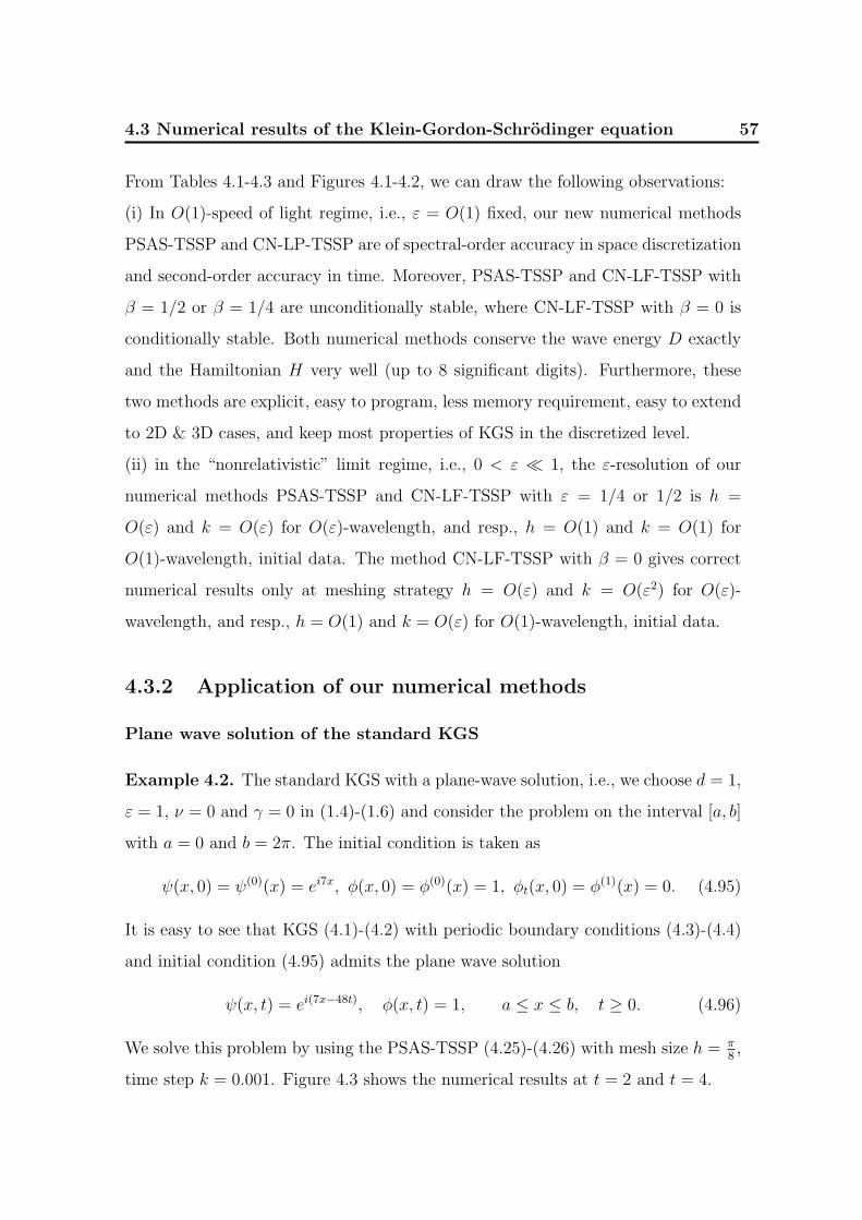
4.3 Numerical results of the Klein-Gordon-Schrodinger equation 57
From Tables 4.1-4.3 and Figures 4.1-4.2, we can draw the following observations:
(i) In O(1)-speed of light regime, i.e., ε = O(1) fixed, our new numerical methods
PSAS-TSSP and CN-LP-TSSP are of spectral-order accuracy in space discretization
and second-order accuracy in time. Moreover, PSAS-TSSP and CN-LF-TSSP with
β = 1/2 or β = 1/4 are unconditionally stable, where CN-LF-TSSP with β = 0 is
conditionally stable. Both numerical methods conserve the wave energy D exactly
and the Hamiltonian H very well (up to 8 significant digits). Furthermore, these
two methods are explicit, easy to program, less memory requirement, easy to extend
to 2D & 3D cases, and keep most properties of KGS in the discretized level.
(ii) in the “nonrelativistic” limit regime, i.e., 0 < ε ¿ 1, the ε-resolution of our
numerical methods PSAS-TSSP and CN-LF-TSSP with ε = 1/4 or 1/2 is h =
O(ε) and k = O(ε) for O(ε)-wavelength, and resp., h = O(1) and k = O(1) for
O(1)-wavelength, initial data. The method CN-LF-TSSP with β = 0 gives correct
numerical results only at meshing strategy h = O(ε) and k = O(ε2) for O(ε)-
wavelength, and resp., h = O(1) and k = O(ε) for O(1)-wavelength, initial data.
4.3.2 Application of our numerical methods
Plane wave solution of the standard KGS
Example 4.2. The standard KGS with a plane-wave solution, i.e., we choose d = 1,
ε = 1, ν = 0 and γ = 0 in (1.4)-(1.6) and consider the problem on the interval [a, b]
with a = 0 and b = 2π. The initial condition is taken as
ψ(x, 0) = ψ(0)(x) = ei7x, φ(x, 0) = φ(0)(x) = 1, φt(x, 0) = φ(1)(x) = 0. (4.95)
It is easy to see that KGS (4.1)-(4.2) with periodic boundary conditions (4.3)-(4.4)
and initial condition (4.95) admits the plane wave solution
ψ(x, t) = ei(7x−48t), φ(x, t) = 1, a ≤ x ≤ b, t ≥ 0. (4.96)
We solve this problem by using the PSAS-TSSP (4.25)-(4.26) with mesh size h = π8,
time step k = 0.001. Figure 4.3 shows the numerical results at t = 2 and t = 4.

4.3 Numerical results of the Klein-Gordon-Schrodinger equation 58
(a)−30 0 300
1
2
3
4
5
6
7
x−30 0 300
1
2
3
4
5
6
7
8
9
10
x
(b)−30 0 300
1
2
3
4
5
6
7
x−30 0 300
1
2
3
4
5
6
7
8
9
10
x
(c)−30 0 300
1
2
3
4
5
6
7
x−30 0 300
1
2
3
4
5
6
7
8
9
10
x
Figure 4.1: Numerical solutions of the meson field φ (left column) and the nucleon
density |ψ|2 (right column) at t = 1 for Example 1 with Type 1 initial data in the
“nonrelativistic” limit regime by PSAS-TSSP. ’-’: exact solution given in (4.96), ‘+
+ +’: numerical solution. I. With the meshing strategy h = O(ε) and k = O(ε):
(a) Γ0 = (ε0, h0, k0) = (0.125, 0.25, 0.04), (b) Γ0/4, and (c) Γ0/16.
From Figure 4.3, we can see that the PSAS-TSSP method for KGS really provides
the exact plane-wave solution of the KGS equations (4.1)-(4.5).
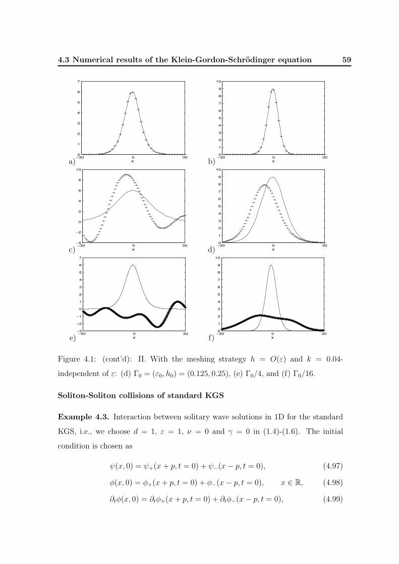
4.3 Numerical results of the Klein-Gordon-Schrodinger equation 59
a)−30 0 300
1
2
3
4
5
6
7
x b)−30 0 300
1
2
3
4
5
6
7
8
9
10
x
c)−30 0 30
−4
−2
0
2
4
6
8
10
x d)−30 0 300
1
2
3
4
5
6
7
8
9
10
x
e)−30 0 30
−3
−2
−1
0
1
2
3
4
5
6
7
x f)−30 0 300
1
2
3
4
5
6
7
8
9
10
x
Figure 4.1: (cont’d): II. With the meshing strategy h = O(ε) and k = 0.04-
independent of ε: (d) Γ0 = (ε0, h0) = (0.125, 0.25), (e) Γ0/4, and (f) Γ0/16.
Soliton-Soliton collisions of standard KGS
Example 4.3. Interaction between solitary wave solutions in 1D for the standard
KGS, i.e., we choose d = 1, ε = 1, ν = 0 and γ = 0 in (1.4)-(1.6). The initial
condition is chosen as
ψ(x, 0) = ψ+(x + p, t = 0) + ψ−(x− p, t = 0), (4.97)
φ(x, 0) = φ+(x + p, t = 0) + φ−(x− p, t = 0), x ∈ R, (4.98)
∂tφ(x, 0) = ∂tφ+(x + p, t = 0) + ∂tφ−(x− p, t = 0), (4.99)

4.3 Numerical results of the Klein-Gordon-Schrodinger equation 60
a) −40 0 40−0.1
0
0.1
0.2
0.3
0.4
0.5
0.6
0.7
b) −30 0 300
0.1
0.2
0.3
0.4
0.5
0.6
0.7
0.8
c) −30 0 30−0.1
0
0.1
0.2
0.3
0.4
d) −30 0 300
0.1
0.2
0.3
0.4
0.5
0.6
0.7
0.8
e) −30 0 30−0.05
0
0.1
0.2
0.3
0
0.4
0.5
f) −30 0 300
0.1
0.2
0.3
0.4
0.5
0.6
0.7
0.8
Figure 4.2: Numerical solutions of the density |ψ(x, t)|2 and the meson field φ(x, t)
at t = 1 in the nonrelativistic limit regime by PSAS-TSSP with the same mesh
(h = 1/2 and k = 0.005). ’-’: ‘exact’ solution , ’+ + +’: numerical solution. The
left column corresponds to the meson field φ(x, t): (a) ε = 1/2, (c) ε = 1/16. (e)
ε = 1/128. The right column corresponds to the density |ψ(x, t)|2: (b) ε = 1/2, (d)
ε = 1/16. (f) ε = 1/128.
where ψ± and φ± are defined as in (3.41) and (3.42), and x = ±p are initial locations
of the two solitons.

4.3 Numerical results of the Klein-Gordon-Schrodinger equation 61
a) 0 1 2 3 4 5 6
−1
−0.5
0
0.5
1
x
Re(ψ
(x,t)
)
0 1 2 3 4 5 6
−1
−0.5
0
0.5
1
x
Re(ψ
(x,t)
)
b)0 1 2 3 4 5 6
−1
−0.5
0
0.5
1
x
Im(ψ
(x,t)
)
0 1 2 3 4 5 6
−1
−0.5
0
0.5
1
x
Im(ψ
(x,t)
)
c)0 1 2 3 4 5 6
0
0.5
1
1.5
2
x
φ(x,t
)
0 1 2 3 4 5 60
0.5
1
1.5
2
x
φ(x,t
)
Figure 4.3: Numerical solutions for plane wave of KGS in Example 4.2 at time t = 2
(left coumn) and t = 4 (right column). ’–’: exact solution given in (4.96), ’+ + +’:
numerical solution. (a): Real part of nucleon filed Re(ψ(x, t)); (b): imaginary part
of nucleon field Im(ψ(x, t)); (c): meson filed φ.
We solve the problem in the interval [−40, 40], i.e., a = −40 and b = 40 with mesh
size h = 5/128 and time step k = 0.001 by using our method PSAS-TSSP, and take
p = 8 and B = 1. Figure 4.4 shows the values of |ψ(x, t)| and φ(x, t) at different
times. From Figure 4.4, the time t = 9.2 corresponds to the time when the two
solitons are at the same location and the time t = 18.5 corresponds to the time
when the collision is nearing completion (cf. Figure 4.4). From the figure we can
see that during the collision, waves are emitted, and that after the collision the two

4.3 Numerical results of the Klein-Gordon-Schrodinger equation 62
0
1
2
3
|ψ|t=0.0
0
1
2
3
|ψ|
t=7.8
0
1
2
3
4
5
|ψ|
t=8.8
0
1
2
3
4
5
|ψ|
t=9.2
0
1
2
3
|ψ|
t=10.2
0
1
2
3
|ψ|
t=11.2
−10 −5 0 5 100
1
2
3
x
|ψ|
t=12.5
−10 −5 0 5 100
1
2
3
x
|ψ|
t=18.5
Figure 4.4: Numerical solutions of soliton-soliton collison in standard KGS in Ex-
ample 4.3 I: Nucleon density |ψ(x, t)|.
solitons have a reduced peak value.
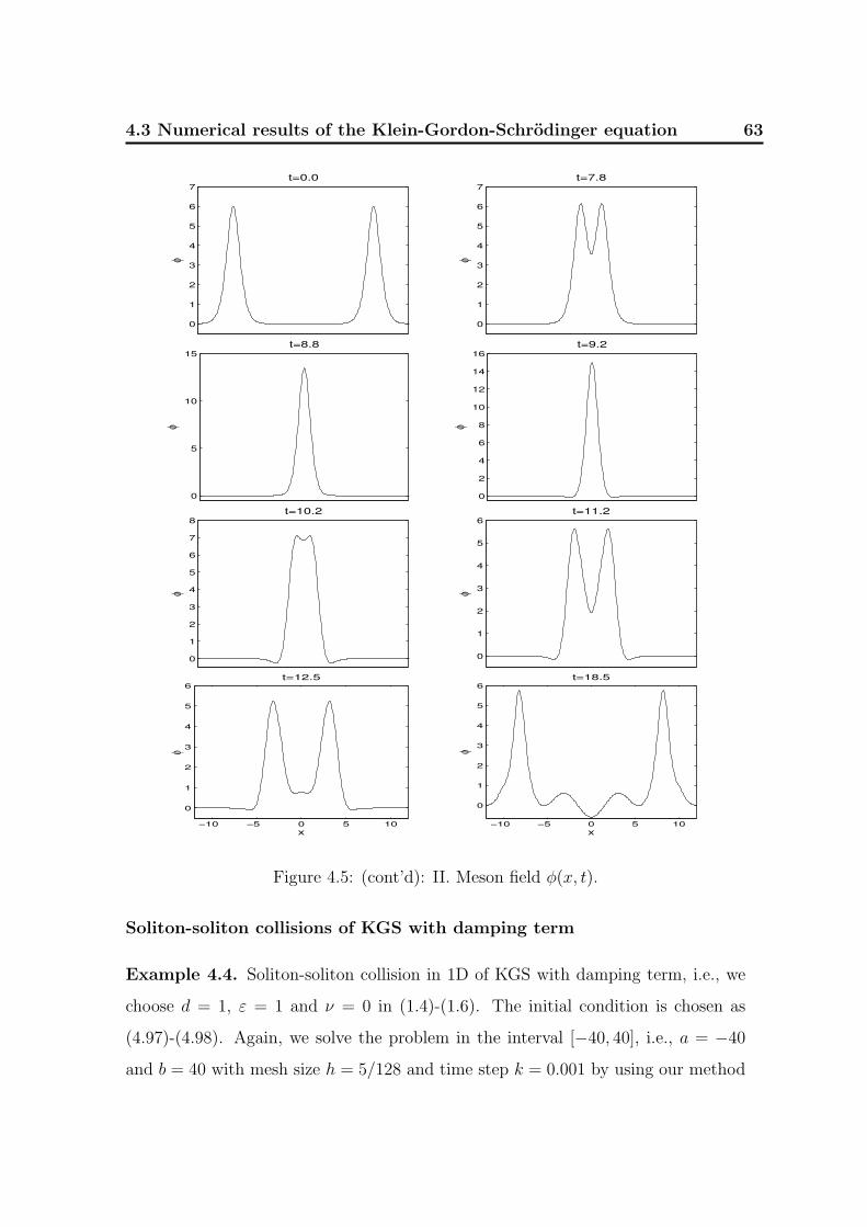
4.3 Numerical results of the Klein-Gordon-Schrodinger equation 63
0
1
2
3
4
5
6
7φ
t=0.0
0
1
2
3
4
5
6
7
φ
t=7.8
0
5
10
15
φ
t=8.8
0
2
4
6
8
10
12
14
16
φ
t=9.2
0
1
2
3
4
5
6
7
8
φ
t=10.2
0
1
2
3
4
5
6
φ
t=11.2
−10 −5 0 5 10
0
1
2
3
4
5
6
x
φ
t=12.5
−10 −5 0 5 10
0
1
2
3
4
5
6
x
φ
t=18.5
Figure 4.5: (cont’d): II. Meson field φ(x, t).
Soliton-soliton collisions of KGS with damping term
Example 4.4. Soliton-soliton collision in 1D of KGS with damping term, i.e., we
choose d = 1, ε = 1 and ν = 0 in (1.4)-(1.6). The initial condition is chosen as
(4.97)-(4.98). Again, we solve the problem in the interval [−40, 40], i.e., a = −40
and b = 40 with mesh size h = 5/128 and time step k = 0.001 by using our method

4.3 Numerical results of the Klein-Gordon-Schrodinger equation 64
PSAS-TSSP, and take p = 8 and B = 1. Figure 4.6 displays time evolution of
|ψ(x, t)|2 and φ(x, t) for different values of γ. Figure 4.7 shows time evolution of the
Hamiltonian H(t) and mean value of the meson field N(t) for different values of γ.
From Figures 4.6-4.7, we can draw the following conclusions: (i) When γ = 0, the
collision between two solitons seems quite elastic (cf. Figure 4.6 top row) although
there are some waves are emitted; when γ > 0 but small, damping effect can be
observed in the collision and the emission of the sound waves is inconspicuous; when
γ > 0 and large, a soliton wave which is a bound state of the KGS is generated
after the collision (cf. 4.6 3 last row). This observation seems new for the KGS. (ii).
When γ = 0, the Hamiltonian is conserved; when γ > 0, it decreases when time
increases and converges to a constant when time goes infty (cf. Figure 4.7 left).
(iii) When γ = 0, the mean value of the meson field changes periodically; where
it oscillates and decays when γ > 0 (cf. Figure 4.7 right). These agree very well
with the analytical results in section 2. (iv) The results here also demonstrate the
efficiency and high resolution of our numerical method for studying soliton-soliton
collision in KGS.
Soliton-soliton collisions of KGS in “nonrelativistic limit” regime
Example 4.5. Soliton-soliton collision in 1D of KGS in “nonrelativistic limit”
regime, i.e., we choose d = 1, γ = 0 and ν = 0 in (1.4)-(1.6). Let
ψ(0)(x) = sech(x + p)e−2i(x+p) + sech(x− p)e−2i(x−p), (4.100)
φ(0)(x) = −|sech(x + p)|2 − |sech(x− p)|2, x ∈ R. (4.101)
We solve the KGS (1.4)-(1.6) in one dimension with the initial conditions
ψKGS(x, 0) = ψ(0)(x), φKGS(x, 0) = φ(0)(x), ∂tφKGS(x, 0) = 0, x ∈ R, (4.102)
in the interval [−128, 128]. We take p = 16.0. Figures 4.9-4.10 show that there are
many oscillations when ε → 0, which are quite different from the numerical results
obtained by the different initial conditions (4.92)-(4.94).

4.3 Numerical results of the Klein-Gordon-Schrodinger equation 65
Figure 4.6: Time evolution of nucleon density |ψ(x, t)|2 (left column) and meson
field φ(x, t) (right column) for soliton-soliton collision of KGS in Example 4.4 for
different values of γ.

4.3 Numerical results of the Klein-Gordon-Schrodinger equation 66
a)0 5 10 15 20 25 30
−30
−20
−10
0
10
20
30
t
H
γ=0γ=0.1γ=1γ=4
b)0 5 10 15 20 25 30
23.999996
23.999998
24.000000
t
N(φ
)
γ=0γ=0.1γ=1γ=4
Figure 4.7: Time evolution of the Hamiltonian H(t) (‘left’) and mean value of the
meson field N(t) (‘right’) in Example 4.4 for different values of γ.
0 2 4 6 8 1031
31.5
32
32.5
33
33.5
34
34.5
35
35.5
36
t
H
γ=0γ=0.1γ=1γ=4
0 2 4 6 8 10−5
0
5
10
t
N(φ
)
γ=0γ=0.1γ=1γ=4
Figure 4.8: Time evolution of the Hamiltonian H(t) (‘left’) and mean value of the
meson field N(t) (‘right’) in Example 4.6 for different values of γ.
Solution of 2D standard KGS
Example 4.6. Dynamics of KGS in 2D, i.e., we choose d = 2, ν = 0 and ε = 1 in
(1.4)-(1.6). The initial condition is taken as
ψ(x, y, 0) =2
ex2+2y2 + e−(x2+2y2)ei5/ cosh(
√4x2+y2),
φ(x, y, 0) = e−(x2+y2), φt(x, y, 0) =e−(x2+y2)
2, (x, y) ∈ R2.

4.3 Numerical results of the Klein-Gordon-Schrodinger equation 67
−40 0 40−0.2
0
0.2
0.4
0.6
0.8
1
1.2
−30 0 300
0.1
0.2
0.3
0.4
−40 0 40
−0.4
−0.2
0
0.2
0.4
0.6
−30 0 300
0.1
0.2
0.3
0.4
0.5
−60 0 60
−0.4
−0.2
0
0.2
0.4
0.6
−30 0 300
0.2
0.4
Figure 4.9: Numerical solutions of the nucleon density |ψ(x, y, t)|2 (right column)
and meson field φ(x, y, t) (left column) in Example 4.5 at t = 1. 1th row: ε = 1/2;
2nd row: ε = 1/8; 3rd row : ε = 1/32.
We solve this problem on the rectangle [−64, 64]2 with mesh size h = 1/16 and time
step k = 0.001 by using our method PSAS-TSSP. Figure 4.11 shows the surface
plots of φ and |ψ|2 with γ = 0 at different times. Figure 4.8 depicts time evolution
of the Hamiltonian H(t) and mean value of the meson field N(t) for different values
of γ.
From Figures 4.8-4.11, we can draw the following conclusions: (i). When γ = 0,
the Hamiltonian is conserved; when γ > 0, it decreases when time increases and

4.3 Numerical results of the Klein-Gordon-Schrodinger equation 68
−40 0 40−0.2
0
0.2
0.4
0.6
0.8
−40 0 200
0.1
0.2
0.3
−40 0 40−0.4
−0.2
0
0.2
0.4
0.6
0.8
−40 0 200
0.2
0.4
−80 0 80−0.4
−0.2
0
0.2
0.4
−30 0 200
0.2
0.4
Figure 4.10: Numerical solutions of the nucleon density |ψ(x, y, t)|2 (right column)
and meson field φ(x, y, t) (left column) in Example 4.5 at t = 2. 1th row: ε = 1/2;
2nd row: ε = 1/8; 3rd row : ε = 1/32.
converges to a constant when time goes infinity (cf. Figure 4.8 left). (ii) When
γ = 0, the mean value of the meson field changes periodically; where it oscillates
and decays when γ > 0 (cf. Figure 4.8 right). These agree very well with the
analytical results in section 2. (iii) The results here also demonstrate the efficiency
and high resolution of our numerical method for studying dynamics of KGS in 2D
& 3D.

4.3 Numerical results of the Klein-Gordon-Schrodinger equation 69
−50
5
−5
0
50
0.2
0.4
0.6
0.8
1
x
t=0
y
Figure 4.11: Surface plots of the nucleon density |ψ(x, y, t)|2 (left column) and meson
field φ(x, y, t) (right column) in Example 4.6 with γ = 0 at different times.

Chapter 5Application to the Schrodinger-Yukawa
equations
In this chapter, we will extend our numerical method, time-splitting spectral method
(TSSP) to the Schrodinger-Yukawa equations and also present the numerical results
of the Schrodinger-Yukawa equations in 1D and 2D cases.
5.1 Introduction to the Schrodinger-Yukawa equa-
tions
The generalized Schrodinger-Yukawa equations are
i η∂tψ = −η2θ∆ψ + Cφψ − α|ψ| 2d ψ − i γψ + Vextψ, x ∈ Rd, t > 0, (5.1)
∆φ = −|ψ|2 + βφ, x ∈ Rd, t > 0, (5.2)
ψ(x, 0) = ψ(0)(x), φ(x, 0) = φ(0)(x), x ∈ Rd. (5.3)
where η is the scaled Planck constant, C > 0 is a fixed constant, α > 0, θ, β are real
parameters and Vext is a given external potential, for example a confining potential.
70

5.1 Introduction to the Schrodinger-Yukawa equations 71
When η = 1, θ = 12, α = 0, Vext = 0, β = 0, we can get the well-known Schrodinger-
Yukawa (S-Y) equations
i ∂tψ + ∆ψ + φψ + i νψ = 0, x ∈ Rd, t > 0, (5.4)
−∆φ + φ = |ψ|2, x ∈ Rd, t > 0; (5.5)
which can be also derived from (1.4) and (1.5) when ε → 0 (corresponding to infinite
speed of light or ‘nonrelativistic’ limit regime).
When θ = 12, γ = 0, β = 0, the system of (5.1) and (5.2) reduces to the well-known
Schrodinger-Poisson-Xα (S-P-Xα) model, which has been firstly derived in [1, 13] as
a local one particle approximation of the time dependent Hartree-Fock equations.
It describes the time evolution of electrons in a quantum model respecting the Pauli
principle in an approximate fashion. It reads
i η∂tψ = −η2
2∆ψ + Cφψ − α|ψ| 2d ψ + Vextψ, x ∈ Rd, t > 0, (5.6)
∆φ = −|ψ|2, x ∈ Rd, t > 0. (5.7)
It is an NLS with two nonlinear terms of different nature: the nonlocal Hartree
potential and a local power term, with focusing sign and an exponent that is sub-
critical for finite time blowup. Such “time dependent density functional theory”
models yield approximations of the time-dependent Hartree-Fock (TDHF) equa-
tions that are much easier to solve numerically: firstly, for large number of particles
N the system of coupled NLS of the TDHF system becomes too large, and secondly,
the exchange terms are very costly to calculate.

5.2 Numerical method for the Schrodinger-Yukawa equations 72
5.2 Numerical method for the Schrodinger-Yukawa
equations
For d = 1, the Schrodinger-Yukawa equations with periodic boundary conditions
can be written as
i η∂tψ = −η2θ∆ψ + Cφψ − α|ψ|2ψ − i νψ + Vextψ, a < x < b, t > 0 (5.8)
∆φ = −|ψ|2 + βφ, a < x < b, t > 0, (5.9)
ψ(a, t) = ψ(b, t), ∂xψ(a, t) = ∂xψ(b, t), t ≥ 0, (5.10)
φ(a, t) = φ(b, t), ∂xφ(a, t) = ∂xφ(b, t), t ≥ 0, (5.11)
ψ(x, 0) = ψ(0)(x), φ(x, 0) = φ(0)(x), a ≤ x ≤ b. (5.12)
The idea to construct the TSSP for the KGS (1.4)-(1.6) can be easily extended to
the Schrodinger-Yukawa equations (5.1)-(5.2). The details of the numerical scheme
are shown below. From time t = tm to t = tm+1, we use the Strang splitting formula:
φm+1j =
1M
∑−M/2≤l≤M/2−1
1µ2
l +β˜(|ψm|2)l eiµl(xj−a), β 6= 0,
1M
∑−M/2≤l≤M/2−1, l 6=0
1µ2
l +β˜(|ψm|2)l eiµl(xj−a), β = 0,
(5.13)
j = 0, 1, 2, · · · ,M − 1. (5.14)
ψ∗j =1
M
M/2−1∑
l=−M/2
e−iηµ2l k/2(ψm)le
iµl(xj−a), j = 0, 1, 2, · · · ,M − 1. (5.15)
ψ∗∗ =
e−i[C(φmj +φm+1
j )/2+Vext(xj)+α(e−2νk−1)|ψ∗j |2/2ν−i ν]k/ηψ∗j , ν 6= 0,
e−i[C(φmj +φm+1
j )/2+Vext(xj)−α|ψ∗j |2−i ν]k/ηψ∗j , ν = 0,(5.16)
j = 0, 1, 2, · · · ,M − 1. (5.17)
ψn+1j =
1
M
M/2−1∑
l=−M/2
eiηµ2l k/2(ψ∗∗)l e
iµl(xj−a), j = 0, 1, 2, · · · ,M − 1; (5.18)
where Ul (l = −M/2, · · · ,M/2 − 1), the Fourier coefficients of a vector U =
(U0, U1, · · · , UM)T with U0 = UM , are defined as
µl =2πl
b− a, Ul =
M−1∑j=0
Uj e−iµl(xj−a), l = −M
2, · · · ,
M
2− 1. (5.19)

5.3 Numerical results of the Schrodinger-Yukawa equations 73
5.3 Numerical results of the Schrodinger-Yukawa
equations
In this section, we study the convergence of KGS to S-Y in the ”nonrelativistic
limit” (0 < ε ¿ 1), where the parameter ε is inversely proportional to the acoustic
speed. We also present the numerical solution of the Schrodinger-Yukawa equations
in the 1D case.
5.3.1 Convergence of KGS to S-Y in “nonrelativistic limit”
regime
Example 5.1. Reduction from the Klein-Gordon-Schrodinger equations to the
Schrodinger-Yukawa equations, i.e., we choose d = 1, ν = 0 and γ = 0 in (1.4)-(1.6).
Let
ψ(0)(x) = sech(x + p)e−2i(x+p) + sech(x− p)e−2i(x−p), (5.20)
and φ(0)(x) satisfies
−φ(0)xx (x) + φ(0)(x) = −|ψ(0)(x)|2. (5.21)
We solve the KGS (1.4)-(1.6) in one dimension with the initial conditions
ψKGS(x, 0) = ψ(0)(x), φKGS(x, 0) = φ(0)(x), ∂tφKGS(x, 0) = 0, x ∈ R, (5.22)
and the S-Y (5.1)-(5.2) in one dimension with the initial condition
ψSY(x, 0) = ψ(0)(x). (5.23)
in the interval [−80, 80] with mesh size h = 5/128 and time step k = 0.00005. We
take p = 8. Let ψKGS and φKGS be the numerical solutions of the KGS (1.4)-(1.6),
ψSY and φSY be of the S-Y (5.1)-(5.2) by using PSAS-TSSP and TSSP respectively.
Table 5.1 shows the errors between the solutions of the KGS and its reduction S-Y
at time t = 1.0 under different ε.

5.3 Numerical results of the Schrodinger-Yukawa equations 74
ε = 1/4 ε/2 ε/4 ε/8
||φKGS − φSY||l2 0.357 3.26E-2 7.762E-3 1.809E-3
||ψKGS − ψSY||l2 3.261E-2 7.597E-3 1.399E-3 3.373E-4
|HKGS −HSY| 0.165 3.314E-2 8.721E-3 2.492E-3
Table 5.1: Error analysis between KGS and its reduction S-Y: Errors are computed
at time t = 1 under h = 5/128 and k = 0.00005.
From Table 5.1, we can see that the meson field φKGS, nucleon density |ψKGS|2, and
the Hamiltonian HKGS of the KGS (1.4)-(1.6) converge to φSY in l2-norm, ψSY in
l2-norm, HSY of the Schrodinger-Yukawa equations (5.1)-(5.2) quadratically when
ε → 0 .
5.3.2 Applications
Example 5.2. 1-D S-P-Xα model, i.e., we choose d = 1, ε = 1, θ = 1/2, Vext ≡ 0
and C = 1 in (5.1)-(5.2). Note that the local interaction term in (5.1) is the “focusing
cubic NLS interaction” in the case d = 1. The initial condition is hence taken the
same as in the simulations of [55]
ψ(x, t = 0) = AI(x)ei SI(x)/ε, x ∈ R, (5.24)
where AI(x) = e−x2, (SI(x))x = −tanh(x). Note that SI is such that the initial phase
is ”compressive”. This means that even the linear evolution develops caustics in
finite time. We solve this problem either on the interval x ∈ [−4, 4] or on x ∈ [−8, 8]
depending on the time for which the solution is calculated.
We present numerical results for four different regimes of α:
Case I. α = 0, i.e., Schrodinger-Poisson regime;
Case II. α = ε, i.e., Schrodinger-Poisson equation with O(ε) cubic nonlinearity;
Case III. α =√
ε, i.e., Schrodinger-Poisson equation with O(√
ε) cubic nonlinearity;

5.3 Numerical results of the Schrodinger-Yukawa equations 75
Case IV. α = 1, i.e., Schrodinger-Poisson equation with O(1) cubic nonlinearity.
Figure 5.1 displays comparisons of the position density n(x, t) = |ψ(x, t)|2 at fixed
time for the above different parameter regimes with different ε. Figure 5.2 plots
the evolution of the position density of the wave function for α = 1 and ε = 0.025.
Figure 5.3 shows the analogous results for the attractive Hartree integration, i.e.,
C = −1, α = 0.5 and ε = 0.025.
From Figure 5.1, we can see that before the break (part a) and b)), the result is
essentially independent of ε. After the break the behavior of the position density
n(x, t) changes substantially with respect to the different regimes of α. For α = 0
the solution stays smooth. For α = ε it also stays smooth, but it concentrates at
the origin. For α =√
ε a pronounced structure of peaks develop, they look like the
soliton structure typical for the NLS [43]. The number of peaks is doubled when ε is
halved. For α = 1, the number of peaks increases again and they occur at different
locations than that for α =√
ε.
We can see that the scaling α = O(√
ε) is critical in the sense that the solution has
a substantially behavior than for the smaller scales of α. Beyond this scaling, the
semiclassical limit can not be obtained by naive numerics.
Figure 5.3 is a test to see what happens if the Hartree potential is attractive instead
of repulsive, with all other parameters kept the same, i.e., Figure 5.2 and Figure 5.3
differ only by the sign of C. The resulting effect corresponds to the physical intuition
that the pattern of caustics that is typical for focusing NLS would be enhanced and
focused in physical space by an additional attractive force.

5.3 Numerical results of the Schrodinger-Yukawa equations 76
a)0 0.2 0.4 0.6 0.8 1 1.2
0
0.2
0.4
0.6
0.8
1
1.2
1.4
1.6
1.8
x
n(x)
Position Density at t=0.25,ε=0.05
α=1α=sqrt(ε)α=εα=0
b)0 0.2 0.4 0.6 0.8 1 1.2
0
0.2
0.4
0.6
0.8
1
1.2
1.4
1.6
1.8Position Density at t=0.25,ε=0.0125
x
n(x)
α=1α=sqrt(ε) α=ε α=0
c)0 1 2 3 4 5
0
0.5
1
1.5
2
2.5
3
3.5Position Density at t=4.0,ε=0.1
x
n(x)
α=1α=sqrt(ε)α=εα=0
d)0 1 2 3 4 5 6
0
0.5
1
1.5
2
2.5
3
3.5
4
4.5
5Position Density at t=4.0,ε=0.05
x
n(x)
α=1α=sqrt(ε)α=εα=0
e)0 1 2 3 4 5 6
0
1
2
3
4
5
6Position Density at t=4.0,ε=0.0375
x
n(x)
α=1α=sqrt(ε)α=εα=0
f)0 1 2 3 4 5 6
0
1
2
3
4
5
6Position Density at t=4.0,ε=0.025
x
n(x)
α=1α=sqrt(ε)α=εα=0
Figure 5.1: Numerical results for different scales of the Xα term in Example 5.2,
i.e., α = 1,√
ε, ε, 0. a) and b) : small time t = 0.25, pre-break, a) for ε = 0.05, b)
for ε = 0.0125. c)-f): large time, t = 4.0, post-break. c) for ε = 0.1, d) for ε = 0.05,
e) for ε = 0.0375, f) ε = 0.025.

5.3 Numerical results of the Schrodinger-Yukawa equations 77
x
t0 0.5 1
3.5
2.5
1.5
0.5
Figure 5.2: Time evolution of the position density for Xα term at O(1) in Example
5.2, i.e., α = 0.5, with ε = 0.025, h = 1/512 and k = 0.0005. a) surface plot; b)
pseudocolor plot.
a) b) x
t
0 0.2 0.4 0.6 0.80
0.5
1
1.5
2
2.5
3
3.5
4
Figure 5.3: Time evolution of the position density for attractive Hartree interaction
in Example 5.2. C = −1, α = 0.5, ε = 0.025, k = 0.00015. a) surface plot; b)
pseudocolor plot.

Chapter 6Conclusion
We began with the derivation of the Klein-Gordon equation (KG) which describes
scalar (or pseudoscalar) spinless particles and analyzed its properties and presented
Crank-Nicolson leap-frog spectral method (CN-LF-SP) for numerical discretization
of the nonlinear Klein-Gordon equation. Numerical results for the Klein-Gordon
equation demonstrated that the method is of spectral-order accuracy in space and
second-order accuracy in time and it is much better than the other numerical meth-
ods proposed in the literature. It also preserves the system energy, linear momentum
and angular momentum very well in the discretized level.
We continued with the derivation of the Klein-Gordon-Schrodinger equations (KGS)
which describes a system of conserved scalar nucleons interacting with neutral scalar
mesons coupled through the Yukawa interaction and analyzed its properties. Two
new and efficient numerical methods are proposed for numerical discretization of the
Klein-Gordon-Schrodinger equations. They are phase space analytical solver+time-
splitting spectral method (PSAS-TSSP) and Crank-Nicolson leap-frog time-splitting
spectral method (CN-LF-TSSP). These methods are explicit, unconditionally sta-
ble, of spectral accuracy in space and second order accuracy in time, easy to extend
to high dimensions, easy to program, less memory-demanding, and time reversible
and time transverse invariant. Furthermore, they conserve (or keep the same decay
78

79
rate of) the wave energy in KGS when there is no damping (or a linear damping)
term, give exact results for plane-wave solutions of KGS, and keep the same dynam-
ics of the mean value of the meson field in discretized level. We also applied our
new numerical methods to study numerically soliton-soliton interaction of KGS in
1D and dynamics of KGS in 2D. We numerically found that, when a large damping
term is added to the Klein-Gordon equation, bound state of KGS can be obtained
from the dynamics of KGS when time goes to infinity.
Finally, we extended our numerical method, time-splitting spectral method (TSSP)
to the Schrodinger-Yukawa equations and presented the numerical results of the
Schrodinger-Yukawa equations in 1D and 2D cases.
Bibliography
[1] M.J. Ablowitz and P.A. Clarkson, Solitons, nonlinear evolution equations and
inverse scattering, Cambridge University Press, London, 1991.
[2] M.J. Ablowitz, B.M. Herbst and C. Schober, On the numerical solution of the
sine-Gordon equation, J. Comput. Phys., 126 (1996), pp. 299-314.
[3] M.J. Ablowitz, M.D. Kruskal and J.F. Ladik, Solitary wave collisions, SIAM
J. Appl. Math., 36 (1979), pp. 428-437.
[4] J. Argyris, M. Haase and J.C. Heinrich, Finite element approximation to two-
dimensional sine-Gordon solitons, Comput. Methods Appl. Mech. Eng., 86
(1991), pp. 1-26.
[5] W. Bao and D. Jaksch, An explicit unconditionally stable numerical method
for solving damped nonlinear Schrodinger equations with a focusing nonlin-
earity, SIAM J. Numer. Anal., 41 (2003), pp. 1406-1426.
[6] W. Bao, D. Jaksch and P.A. Markowich, Numerical solution of the Gross-
Pitaevsikii equation for Bose-Einstein condensation, J. Comput. Phys., 187
(2003), pp. 318-342.
80

Bibliography 81
[7] W. Bao, D. Jaksch and P.A. Markowich, Three Dimensional Simulation of Jet
Formation in Collapsing Condensates, J. Phys. B: At. Mol. Opt. Phys., 37
(2004), pp. 329-343.
[8] W. Bao, S. Jin and P.A. Markowich, On time-splitting spectral approximations
for the Schrodinger equation in the semiclassical regime, J. Comput. Phys., 175
(2002), pp. 487-524.
[9] W. Bao, S. Jin and P.A. Markowich, Numerical study of time-splitting spectral
discretizations of nonlinear Schrodinger equations in the semiclassical regimes,
SIAM J. Sci. Comput., 25 (2003), pp. 27-64.
[10] W. Bao and X.G. Li, An efficient and stable numerical method for the Maxwell-
Dirac system, J. Comput. Phys., 199 (2004), pp. 663-687.
[11] W. Bao, F.F. Sun and G.W. Wei, Numerical methods for the generalized
Zakharov system, J. Comput. Phys., 190 (2003), pp. 201-228.
[12] W. Bao and F.F. Sun, Efficient and stable numerical methods for the gen-
eralized and vector Zakharov system, SIAM J. Sci. Comput., 26 (2005), pp.
1057-1088.
[13] C. Bardos, F. Golse and N.J. Mauser, Weak coupling limit of the N-particle
Schrodinger equation, Math. Analysis and Application, 7 (2000), pp. 275-293.
[14] A. Barone, F. Esposito, C.J. Magee and A.C. Scott, Theory and applications
of the sine-Gordon equation, Riv. Nuovo Cimento, 1 (1971), pp. 227-267.
[15] P. Bechouche, N.J. Mauser and S. Selberg, Non-relativistic limit of Klein-
Gordon-Maxwell, American J. of Math., 126 (2004), pp. 31-64.
[16] P. Bechouche, N.J. Mauser and S. Selberg, Nonrelativistic limit of Klein-
Gordon-Maxwell to Schrodinger-Poisson, preprint.

Bibliography 82
[17] P. Biler, Attractors for the system of Schrodinger and Klein-Gordon equations
with Yukawa coupling, SIAM J. Math. Anal., 21 (1990), pp. 1190-1212.
[18] J.G. Caputo, N. Flytzanis and Y. Gaididei, Split mode method for the el-
liptic 2D sine-Gordon equation: application to Josephson junction in overlap
geometry, Int. J. Mod. Phys. C, 9 (1998), pp. 301-323.
[19] P.L. Christiansen and P.S. Lomdahl, Numerical study of 2+1 dimensional sine-
Gordon solitons, Physica D, 2 (1981), pp. 482-494.
[20] R.J. Cirincione and P.R. Chernoff, Dirac and Klein-Gordon equations: con-
vergence of solutions in the nonrelativistic limit, Commun. Math. Phys., 79
(1981), pp. 33-46.
[21] C. Dariescu and M.A. Dariescu, Transition and regeneration rates in charged
boson stars via perturbative calculations, Int. Journal of Modern Phy. A, 20
(2005), pp. 2326-2330.
[22] A. Darwish and E.G. Fan, A series of new explicit exact solutions for the
coupled Klein-Gordon-Schrodinger equations, Chaos, Solitons & Fractals, 20
(2004), pp. 609-617.
[23] R.F. Dashen, B. Hasslacher and A. Neuveu, Nonperturbative methods and ex-
tended hadron models in field theory II. Two-dimensional model and extended
hadrons, Phys. Rev. D, 10 (1974), pp. 4130-4138.
[24] K. Djidjeli, W.G. Price and E.H. Twizell, Numerical solutions of a damped
sine-Gordon equation in two space variables, J. Eng. Math., 29 (1995), pp.
347-369.
[25] R.K. Dodd, J.C. Eilbeck, J.D. Gibbon and H.C. Morris, Solitons and nonlinear
wave equations, Academic Press, London, 1982.
[26] B. Fornberg and T.A. Driscoll, A fast spectral algorithm for nonlinear wave
equations with linear disperision, J. Comput. Phys. 155 (1999), pp. 456-467.

Bibliography 83
[27] F. Fucito, F. Marchesoni, E. Marinari, G. Parisi, L. Peliti, S. Ruffo and
A. Vulpiani, Approach to equilibrium in a chain of nonlinear oscillators, J.
Physique, 43 (1982), pp. 707-713.
[28] I. Fukuda and M. Tsutsumi, On the Yukawa-coupled Klein-Gordon-
Schrodinger equations in three space dimensions, Proc. Japan Acad., 51 (1975),
pp. 402-405.
[29] I. Fukuda and M. Tsutsumi, On coupled Klein-Gordon-Schrodinger equations
II, J. Math. Anal. Appl., 66 (1978), pp. 358-378.
[30] I. Fukuda and M. Tsutsumi, On coupled Klein-Gordon-Schrodinger equations
III, Math. Japan, 24 (1979), pp. 307-321.
[31] J.D. Gibbon, I.N. James and I.M. Moroz, The sine-Gordon equation as a model
for a rapidly rotating baroclinic fluid, Phys. Scripta, 20 (1979), pp. 402-408.
[32] J. Ginibre and G. Velo, The global Cauchy problem for the nonlinear Klein-
Gordon equation, Math. Z., 189 (1985), pp. 487-505.
[33] B.L. Guo, Global solution for some problem of a class of equations in interac-
tion of complex Schrodinger field and real Klein-Gordon field, Sci. China Ser.
A, 25 (1982), pp. 97-107.
[34] B.L. Guo and C.X. Miao, Asymptotic behavior of coupled Klein-Gordon-
Schrodinger equations, Sci. China Ser. A, 25 (1995), pp. 705-714.
[35] B.L. Guo and Y.S. Li, Attractor for dissipative Klein-Gordon-Schrodinger
equations in R3, J. Diff. Eq., 136 (1997), pp. 356-377.
[36] B.Y. Guo, X. Li and L. Vazquez, A Legendre spectral method for solving the
nonlinear Klein-Gordon equation, Comput. Appl. Math., 15 (1996), pp. 19-36.
[37] N. Hayashi and W. von Wahl, On the global strong solutions of coupled Klein-
Gordon-Schrodinger equations, J. Math. Soc. Jpn., 39 (1987), pp. 489-497.

Bibliography 84
[38] F.T. Hioe, Periodic solitary waves for two coupled nonlinear Klein-Gordon and
Schrodinger equations, J. Phys. A: Math. Gen., 36 (2003), pp. 7307-7330.
[39] Z. Huang, S. Jin, P.A. Markowich, C. Sparber and C. Zheng, A time-splitting
spectral scheme for the Maxwell-Dirac system, J. Comput. Phys., 208 (2005),
pp. 761–789.
[40] S. Jimenez and L. Vazquez, Analysis of four numerical shcemes for a nonlinear
Klein-Gordon equation, App. Math. Comput., 35 (1990), pp. 61-94.
[41] S. Jimenez, Comportamiento de Ciertas Cadenas de Osciladores No Lineales,
Ph.D. Thesis, Univ. Complutense de Madrid, Spain, 1988.
[42] S. Jin, P.A. Markowich and C. Zheng, Numerical simulation of a generalized
Zakharov system, J. Comput. Phys., 201 (2004), pp. 376–395.
[43] , S. Kamvissis, K.T.R. McLaughlin and P.D. Miller, Semiclassical soliton en-
sembles for the focusing nonlinear Schrodinger equation, Annals of Mathemat-
ics Studies 154, Princeton University Press, Princeton, 2003.
[44] D. Kaya, An implementation of the ADM for generalized one-dimensional
Klein-Gordon equation, Appl. Math. Comput., 166 (2005), pp. 426-433.
[45] M.E. Khalifa and M. Elgamal, A numerical solution to Klein-Gordon equation
with Dirichlet boundary condition, Appl. Math. Comput., 160 (2005), pp. 451-
475.
[46] A.Q.M. Khaliq, B. Abukhodair and Q. Sheng, A predictorCcorrector scheme
for the sine-Gordon equation, Numer. Methods Partial Differ. Eqns., 16 (2000),
pp. 133-146.
[47] K.R. Khusnutdinova and D.E. Pelinovsky, On the exchange of energy in cou-
pled Klein-Gordon equations, Wave Motion, 38 (2003), pp. 1-10.

Bibliography 85
[48] O.M. Kiselev, Perturbation of a solitarywave of the nonlinear KleinCGordon
equation, Siberian Math. J., 41 (2000), pp. 345-358.
[49] G.L. Lamb, Elements of soliton theory, Wiley, New York, 1980.
[50] Y. Li and B. Guo, Asymptotic smoothing effect of solutions to weakly dissiptive
Klein-Gordon-Schrodinger equations, J. Math. Annl. Appl., 282 (2003), pp.
256-265.
[51] X.Q. Liu and S. Jiang, Exact solutins of multi-component nonlinear
Schrodinger and Klein-Gordon equations, Appl. Math. Comp., 160 (2005),
pp. 875-880.
[52] X. Lu and R. Schmid, Symplectic integration of sine-Gordon type systems,
Math. Comput. Simul., 50 (1999), pp. 255-263.
[53] K.N. Lu and B.X. Wang, Global attractors for the Klein-Gordon-Schrodinger
equation in unbounded domains, J. Diff. Eq., 170 (2001), pp. 281-316.
[54] V.G. Makhankov, Dynamics of classical solitons (in non-integrable systems),
Phys. Lett. C, 35 (1978), pp. 1-128.
[55] P. Miller and S. Kamvissis, On the semiclassical limit of the focusing nonlinear
Schrodinger equation, Phys. Lett. A, 247 (1998), pp. 75-86.
[56] M. Ohta, Stability of stationary states for the coupled Klein-Gordon-
Schrodinger equations, Non. Anal., 27 (1996), pp. 455-461.
[57] T. Ozawa, K. Tsutaya and Y. Tsutsumi, Well-posedness in energy space for
the Cauchy problem of the Klein-Gordon-Zakharov equations with different
propagation speeds in three space dimensions, Math. Ann., 313 (1999), pp.
127-140.

Bibliography 86
[58] T. Ozawa, and Y. Tsutsumi, Asymptotic behaviour of solutions for the coupled
Klein-Gordon-Schrodinger equations, Adv. Stud. Pure Math., 23 (1994), pp.
295-305.
[59] A.C. Scott, Active and nonlinear wave propagation in electronics, Springer,
New York, 1978.
[60] R. Shankar, Principles of quantum mechanics, Kluwer Academic/Plenum Pub-
lishers, New York.
[61] G. Strang, On the construction and comparison of difference schemes, SIAM
J. Numer. Anal., 5 (1968), pp. 505-517.
[62] W.A. Strauss and L. Vazquez, Numerical solution of a nonlinear Klein-Gordon
equation, J. Comput. Phys., 28 (1978), pp. 271-278.
[63] T.R. Taha and M.J. Ablowitz, Analytical and numerical aspects of certain
nonlinear evolution equations,III. Numerical, nonlinear Schrodinger equation,
J. Comput. Phys., 55 (1984), pp. 203-230.
[64] K. Veselic, On the nonrelativistic limit of the bound states of the Klein-Gordon
equation, J. Math. Anal. Appl., 96 (1983), pp. 63-84.
[65] Q.F. Wang and D.Z. Cheng, Numerical solution of damped nonlinear Klein-
Gordon equations using variational method and finite element approach, Appl.
Math. Comput., 162 (2005), pp. 381-401.
[66] Y.H. Wang, B. Wang, High-order multi-symplectic schemes for the nonlinear
Klein-Gordon equation, Appl. Math. Comput., 166 (2005), pp. 608-632.
[67] M.L. Wang and Y.B. Zhou, The periodic wave solutions for the Klein-Gordon-
Schrodinger equations, Phys. Lett. A, 318 (2003), pp. 84-92.
[68] R.A. Weder, Scattering theory for the Klein-Gordon equation, J. Functional
Analysis, 27 (1978), pp. 100-117.

Bibliography 87
[69] X.M. Xiang, Spectral method for solving the system of equations of
Schrodinger-Klein-Gordon field, J. Comput. Appl. Math., 21 (1988), pp. 161-
171.
[70] L.M. Zhang, Convergence of a conservative difference scheme for a class of
Klein-Gordon-Schrodinger equations in one space dimension Appl. Math. Com-
put., 163 (2005), pp. 343-355.