numerical solution of sobolev partial differential...

SIAM J. NUMER. ANAL.Vol. 12, No. 3, June 1975

NUMERICAL SOLUTION OF $OBOLEV PARTIALDIFFERENTIAL EQUATIONS*

RICHARD E. EWING-

Abstract. Finite difference techniques can be applied to the numerical solution of the initial-boundary value problem in S for the semilinear Sobolev or pseudo-parabolic equation

(xiUt "-b b u q ru

where ai, bi, q and are functions of space and time variables, q is a boundedly differentiable functionof u, and S is an open, connected domain in [R". Under suitable smoothness conditions, the solution ofa Crank-Nicolson type of difference equation is shown to converge to u in the discrete L2-norm withan O((Ax) + (At)2) discretization error.

The numerical problem is reduced to the inversion of a certain matrix at each time level. For theproblem with constant coefficients in a two- or three-dimensional cube, a two-level iteration schemewith a Picard-type outer iteration and an alternating direction inner iteration is presented. For moregeneral operators and more general regions in N" for arbitrary n the same two-level scheme with a

successive overrelaxation inner iteration is discussed.

1. Introduction. The purpose of this paper is to consider the numericalsolution of certain partial differential equations with one time derivative appearingin the highest order terms. Equations of this type arise in many areas of mathe-matics and physics. They are used to study consolidation of clay [25], heat con-duction 2], homogeneous fluid flow in fissured material 13, shear in secondorder fluids 3], 18] and other physical models. In connection with nonsteadyflow of second order fluids, Ting I26] considers the initial-boundary value problemfor the equation

(1.1) pV 1/2aG + CVx., 0 <= x <= h, >= O,

with constant coefficients. For a discussion of several physical applications of thenonlinear problem, see I16.

In a Hilbert space setting, this type of equation is of the form

(1.2) u’(t) + Bu’(t) + Au(t) O, > O,

where A and B are various operators. Yosida used the equation (1.2) with B flAin his proof of the generation theorem for semigroups of operators [28]. The

equation (1.2) with B flA has also been used to approximate certain parabolicequations backward in time I13], [231. In I241, Showalter and Ting discuss theinitial-boundary value problem of the type (1.2) using Hilbert space techniques.Davis [6] and Showalter [21], [22] have also considered various mathematicalaspects of equations of this type. Ford [14] has considered some numerical aspectsof this type of problem.

* Received by the editors January 15, 1974.- Department of Mathematics, Oakland University, Rochester, Michigan 48063. This work was

supported in part by Texas Tech University and by the Center for Numerical Analysis at the Universityof Texas at Austin.

345

Dow

nloa

ded

11/0

9/15

to 1

65.9

1.11

2.14

6. R

edis

trib

utio

n su

bjec

t to

SIA

M li

cens

e or

cop

yrig

ht; s

ee h

ttp://

ww

w.s

iam

.org

/jour

nals

/ojs

a.ph

p

346 RICHARD E. EWING

In this paper we consider linear and semilinear initial-boundary valueproblems in S (0, T] of the form

(a)k=l Xk ak(x, t)u, + bk(X

(1.3)

(b)

(c)

where S

t)-u]}--qu=rut +h,

(xl,..’,x,)eS, O<t<_T,

u(x ,’.’, Xm, 0) f(x ,’", Xm), (X ,’’’, Xm) S,

U(X Xm t) g(X Xm t) (X X,,) e cS O< <= T,

is an open connected subset of Nm and t3S is the boundary of S. We laterdescribe smoothness assumptions and bounds on u and the coefficients above.Standard problems of this type have ai > 0, bi > 0 and r > 0. The backwardtime problems are given by ai > 0, bi < 0 and r > 0. The results of this paperhold for both time cases; however, as we shall see, most of the restrictions on Atcan be dropped when b > 0.

We note that if we limit the number of time levels in the difference equationapproximations to two, the time derivative in the highest order terms necessitatesthe use of implicit numerical schemes. Thus due to the increased rate of con-vergence over standard implicit schemes, we use the m-dimensional analogue ofthe Crank-Nicolson difference equation [5] to replace the differential problem.

In 2 we establish some special notation and present basic assumptionsneeded throughout the paper. In 3 we derive eigenvalue estimates for the prob-lems to be studied in 4 and 5 for fairly general domains and use these to obtainstability. Using the stability analysis and eigenvalue estimates, we derive con-vergence of the Crank-Nicolson difference schemes for the linear problems oftype (1.3) in 4 and for semilinear problems in 5. Finally in 6, we discuss thealgebraic problems for the Crank-Nicolson schemes of the previous sections. Wereduce the problem of convergence to the inversion of a matrix at each timelevel. In order to treat the nonlinear difference equations of 5, we present a pairof two-level iteration schemes. The first method, using an alternating directioninner iteration, applies to equations in a rectangular box with constant co-efficients for m 2 or m 3 and requires calculations of the order

(1.4) O((Ax) log (Ax)- 1)

at each step. The second method, using a successive overrelaxation inner iteration,applies to more general equations in more general regions for arbitrary rn andrequire calculations of the order

(.5) O((Ax)-m+ )at each step.

2. Preliminaries and notation. We shall require some special notation andassumptions. Let 11,12, "", lm be a basis of unit coordinate vectors in Nm. TOset up a finite difference equation, we fix a point (0, 0,.-., 0) and construct arectangular lattice whose nodes are x (x l, x2, "", Xm) such that

(2.1) Xk PkAXk, k 1,2, ..., m,Dow

nloa

ded

11/0

9/15

to 1

65.9

1.11

2.14

6. R

edis

trib

utio

n su

bjec

t to

SIA

M li

cens

e or

cop

yrig

ht; s

ee h

ttp://

ww

w.s

iam

.org

/jour

nals

/ojs

a.ph

p

SOBOLEV PARTIAL DIFFERENTIAL EQUATIONS 347

where Pk 0, +__ 1, +__2,..., and for each k, Axk is the mesh size in the directionlk. We define the average mesh size by

(2.2) Ax= Axmk=l

Two nodes with coordinates pAx and p’Axk are adjacent if ’= (P p,)2 1.The set of nodes in S such that all adjacent nodes belong to S U c3S is the interiorof S denoted Sh. All other nodes in S U c3S belong to the boundary of S U c3Sdenoted c3Sh. We assume S is connected. Also we must make the somewhatstringent assumption that c3Sh cS.

We consider the vector

(2.3) (P l, P2, Pm)

and use the notation for any function f,

(2.4a)

(2.4b)

(2.4c)

f f(plAxi p2Ax2, pmAxm),

f,, f(P 1Ax 1, p2Ax2 ,PmAXm, tn)

+1/2)1k,, f(paAxl "’", P- 1Axe_ 1, (P + 1/2)Axk, p+ 1Axe+ l,

PmAXm, tn)and similarly for f-(1/2)lk,n"

We shall not assume that At equals Axe; however, when we consider S asa cube we assume AXl Ax2 Axm. The standard Landau order notationwill be used. Iff is a function of several variables,

(2.5) f e Ca

(2.6a)

implies that all partial derivatives off of order not greater than fl are continuous.Now we present a list of basic difference formulas we shall use. The proofs

of these formulas follow from Taylor’s theorem.

c(a,),,+ li2 f,,

[(a,)<+(,/2)<,,,+ l/2(f<+h<,,, f,,,,)(a,)<-l/z,,<,.+ 1/2(,,, f-,.)]l(itx<)2 + O((Ax)2),

a< C f C"

(2.6b) f,,+ ,/, (L,,+, + L,,)/2 + O((At)z), f e C2

We shall use standard difference notations [9, pp. 2-4] as well as the notation

(2.7) (A:[a,, +,/2Axf.]), (Ax<[(a,), +li2AxLJL.k=l

Dow

nloa

ded

11/0

9/15

to 1

65.9

1.11

2.14

6. R

edis

trib

utio

n su

bjec

t to

SIA

M li

cens

e or

cop

yrig

ht; s

ee h

ttp://

ww

w.s

iam

.org

/jour

nals

/ojs

a.ph

p


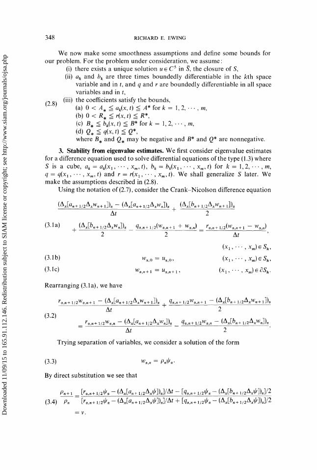
We now make some smoothness assumptions and define some bounds forour problem. For the problem under consideration, we assume:

(i) there exists a unique solution u C in , the closure of S,(ii) ak and bk are three times boundedly differentiable in the kth space

variable and in t, and q and r are boundedly differentiable in all spacevariables and in t,

(2.8) (iii) the coefficients satisfy the bounds,(a) 0 < A, <= a(x, t) <= A* for k 1, 2, ..., m,(b) 0 < R, <__ r(x, t) <__ R*,(c) B, _< bk(X, t) <= B* for k 1, 2, ..., m,(d) Q, q(x, t) <= Q*,where B, and Q, may be negative and B* and Q* are nonnegative.

3. Stability from eigenvalue estimates. We first consider eigenvalue estimatesfor a difference equation used to solve differential equations of the type (1.3) whereS is a cube, a a(x,..., x,,t), b bk(x,..., Xm,t) for k 1,2,..., m,q q(x,..., x,,, t) and r r(xa,..., x,,, t). We shall generalize S later. Wemake the assumptions described in (2.8).

Using the notation of (2.7), consider the Crank-Nicolson difference equation

(Axa,+ 1/2Axw,+ x]) (Ax[a,+ 1/2A,w,])At 2

(Ax[bn+l/2AxWn+l])+

(3.1a) (Ax[b. + 1/2AxWn)ot q=,.+ 1/2(Wa,n+ -- Wot,n) r=,.+ 1/2(Wot,n+ Wa,n)2 2 At

(3.1b)

(3.c)

(x, x,O e &,(x, ..., x) e &,(x ..., x,,) e c&.

Rearranging (3.1a), we have

(3.2)

r,.+ a/2w=,.+ (Ax[a.+ 1/2Axwn+ l)aAt + 2

q=,.+ 1/2Wot,n+ (A,,[b.+ /2Aw.+ 1])

r=,,+ /2w=,, (A,,[a,+ q=,.+ /zw,. (A,,[b.+ 1/2AxWn])aAt 2

Trying separation of variables, we consider a solution of the form

(3.3)

By direct substitution we see that

p.+, [r=,. + ,/20 -(k[a. + ,/2k.4,])=]/At [q=,.+ ,/2’= (Ax[b.+ ,/2AxO])]/2(3.4) [r=,,+ ,/20 -(A[a, + /2AxO])=]/At + [%,,+ ,/2 (Ax[b./ ,/2Ax0])]/2

Dow

nloa

ded

11/0

9/15

to 1

65.9

1.11

2.14

6. R

edis

trib

utio

n su

bjec

t to

SIA

M li

cens

e or

cop

yrig

ht; s

ee h

ttp://

ww

w.s

iam

.org

/jour

nals

/ojs

a.ph

p


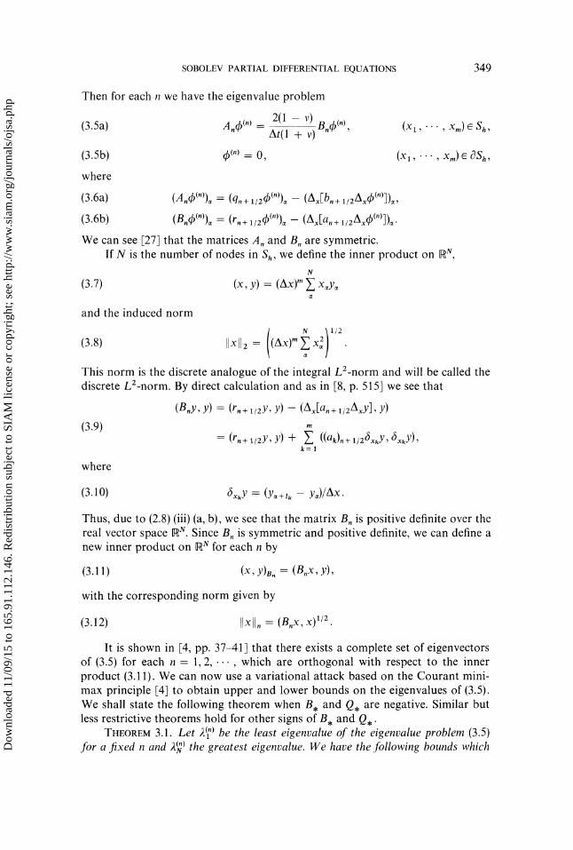
Then for each n we have the eigenvalue problem

(3.5a) A,dp(, 2(1 v)At(1 + v)

(3.5b)

where

(3.6a)

(3.6b)

Bn(n), (x1, Xm) e Sh,

dp (") O, (x ..., x,) e aSh,

(A,49(")) (q,+ 1/2(/)(n))a (A[b,+ /2A4)(")]),(B,qS(")) (r,+ i/2((n))a (A[a,+ i/2Ax(n)J)a.

We can see [27] that the matrices A, and B, are symmetric.If N is the number of nodes in Sh, we define the inner product on

N

(3.7) (x, y) (Ax) xy

and the induced norm

N 1/22Ilxl2 (mx)rn E Xo

This norm is the discrete analogue of the integral L2-norm and will be called thediscrete L2-norm. By direct calculation and as in [8, p. 515] we see that

(B,y, y) (r,,+ 1/2Y, Y) (A,[a,+ 1/2Axy], y)

(3.9)(r.+ 1/2Y, Y) -at- E ((ak).+ 1/2(xkY, (xkY),

k=l

where

(3.1 O) (5,y (y + y)/Ax

Thus, due to (2.8) (iii) (a, b), we see that the matrix B, is positive definite over thereal vector space NN. Since B, is symmetric and positive definite, we can define anew inner product on Nu for each n by

(3.11) (x, Y)n. (B,x, y),

with the corresponding norm given by

(3.12) x (B,x, X) 1/2

It is shown in [4, pp. 37-41] that there exists a complete set of eigenvectorsof (3.5) for each n 1, 2,-.., which are orthogonal with respect to the innerproduct (3.11). We can now use a variational attack based on the Courant mini-max principle [4] to obtain upper and lower bounds on the eigenvalues of (3.5).We shall state the following theorem when B, and Q, are negative. Similar butless restrictive theorems hold for other signs of B, and Q,.

THEOREM 3.1. Let 2(1") be the least eigenvalue of the eigenvalue problem (3.5)for a fixed n and 2 the greatest eigenvalue. We have the following bounds whichD

ownl

oade

d 11

/09/

15 to

165

.91.

112.

146.

Red

istr

ibut

ion

subj

ect t

o SI

AM

lice

nse

or c

opyr

ight

; see

http

://w

ww

.sia

m.o

rg/jo

urna

ls/o

jsa.

php


are uniform in n.

If [Q,[ _>_ (R,IB, I/A,),

(3.13)If ]Q,I < (R,IB,]/A,),

If Q* >= R,IB*[/A,,

If Q* < R,]B*[/A,,

Proof. First we note that as in (3.9),

(.14a)

and

(3.14b)

")_> Q,/R,.

2(") >= B,/A,.) <= O*/R,.),) <__ B*/A,.

(A,dp, 4)) (q,+ ,/2dP, 4)) + ((bk),+ 1/2(m,(,k=l

Therefore for b 4: 0, we see that (A,c, c)l(B,d?, ) is bounded below by

k=l

since Q, and B, are both negative. We note here that since the bounds (2.8) holdfor all t, the bound (3.15) holds for all n. Thus we can obtain uniform bounds onthe eigenvalues by considering the eigenvalue problem

(3.16a) Q, B, PA R, A, Ak=l =1

(3.16b) =0 if(xx,...,x)eOSh.

Therefore, by the Courant minimax principle and a special case of the minimaxtheorem [17, p. 181], we know that

(3.17) 2]") min ti),i= 1,...,N

where t) are the eigenvalues of (3.16). Consider the following rearrangement of(3.16a)"

(3.t8) 2 R-Q,k= A, B,

Since we are working on a cube, Axk Ax for k 1, 2, ..., m, we can let therange from to some M for k 1, 2, ..., m.

Standard arguments [9], [11] yield

4 PkAX(3.19) (Ax)------- sin2

Solving for p, we obtain

(3.20) p[Q, + B,(4/(Ax)2) sin2 (rCpkAX/2)

k=l

[ ]"R, / A,(4/(Ax)2) sin2(xpkAX/2)k=l

Dow

nloa

ded

11/0

9/15

to 1

65.9

1.11

2.14

6. R

edis

trib

utio

n su

bjec

t to

SIA

M li

cens

e or

cop

yrig

ht; s

ee h

ttp://

ww

w.s

iam

.org

/jour

nals

/ojs

a.ph

p


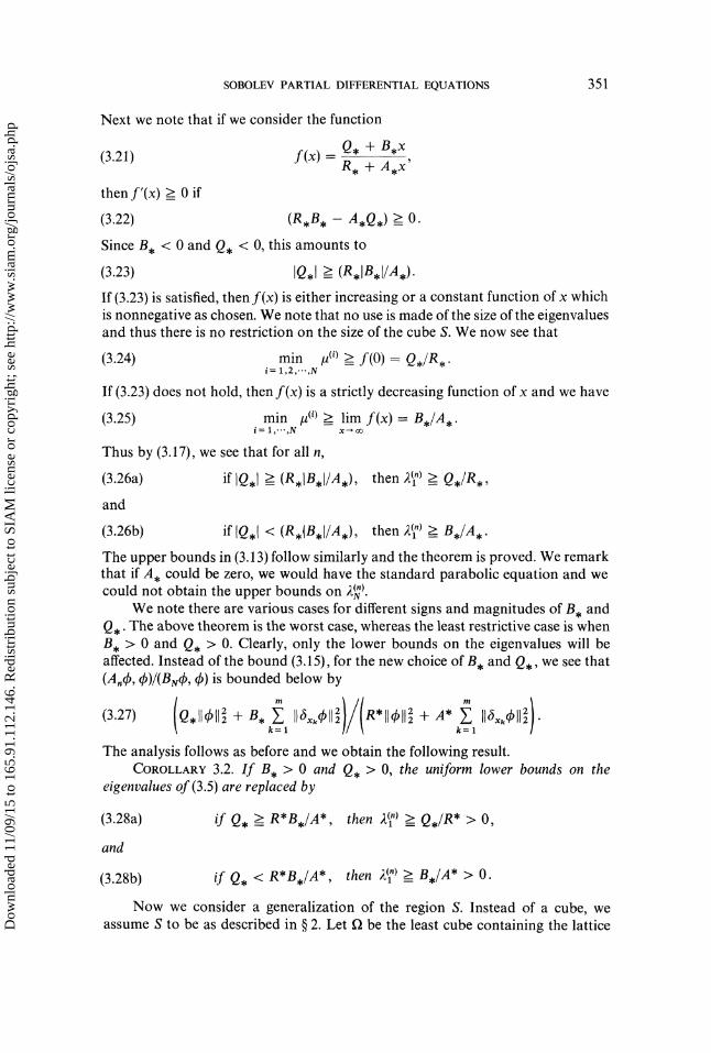
Next we note that if we consider the function

Q, + B,x(3.21) f(x)

R, + A,x’then f’(x) >= 0 if

(3.22) (R,B, A,Q,) >= O,

Since B, < 0 and Q, < 0, this amounts to

(3.23) IQ,I >- (R,IB, I/A,).If (3.23) is satisfied, then f(x) is either increasing or a constant function of x whichis nonnegative as chosen. We note that no use is made of the size of the eigenvaluesand thus there is no restriction on the size of the cube S. We now see that

(3.24) min /i) >__ f(0)= Q,/R,.1,2,...,N

If (3.23) does not hold, then f(x) is a strictly decreasing function of x and we have

(3.25) min /(0>__ lim f(x)= B,/A,.i= 1,-",N x

Thus by (3.17), we see that for all n,

(3.26a) if IO,I _-> (R,IB,I/A,), then 2")>_ Q,/R,,and

(3.26b) if 1(2,1 < (R,IB, I/A,), then 2]")>__ B,/A,.The upper bounds in (3.13) follow similarly and the theorem is proved. We remarkthat if A, could be zero, we would, have the standard parabolic equation and wecould not obtain the upper bounds on 2).

We note there are various cases for different signs and magnitudes of B, andQ,. The above theorem is the worst case, whereas the least restrictive case is whenB, > 0 and Q, > 0. Clearly, only the lower bounds on the eigenvalues will beaffected. Instead of the bound (3.15), for the new choice of B, and Q,, we see that(A,, )/(Budp, ) is bounded below by

(3.27) Q, IlqSll / B, IIx>ll e*ll>ll + A* IIx>ll=1 k=l

The analysis follows as before and we obtain the following result.COROLLARY 3.2. If B, > 0 and Q, > O, the uniform lower bounds on the

eigenvalues of (3.5) are replaced by

(3.28a) if Q, >= R*B,/A*, then 2x") >= Q,/R* > O,

and

(3.28b) if Q, < R*B,/A*, then ;t]") >- B,/A* > O.

Now we consider a generalization of the region S. Instead of a cube, weassume S to be as described in 2. Let f be the least cube containing the latticeD

ownl

oade

d 11

/09/

15 to

165

.91.

112.

146.

Red

istr

ibut

ion

subj

ect t

o SI

AM

lice

nse

or c

opyr

ight

; see

http

://w

ww

.sia

m.o

rg/jo

urna

ls/o

jsa.

php


nodes in S and on cS, and Of be its boundary. It is well known [20, p. 204] thatany matrix corresponding to the operators

(3.29)

Q*-B* Z A2, Q,-B, 2 A2, R*-A* 2 A2,k=l k=l k=l

andk=l

as applied to any lattice region, regardless of the ordering of the points, is sym-metric. Similarly, by direct substitution as in (3.9) we can see that the matricescorresponding to

(3.30) Q*-B* Z AZk and Q,-B, Z AxZkk=l k=l

are positive definite regardless of the ordering of the points. Thus we can orderthe points in Sh first and then order the other points in f. The resulting matricesfor the eigenvalue problem (3.16) will still be positive definite and symmetric asrequired. We can then obtain bounds for the eigenvalues in f as outlined above.Then applying a theorem concerning domination of eigenvalues 20, p. 164]successively on the lattice nodes in f but not in S, we shall retain the same uniformbounds on the eigenvalues for S as for f.

We shall next define the stability of (3.1) with respect to the sequence ofnorms given in (3.12). First we note that (3.2) is actually of the form

(3.31) (C,)w,,+ (D,)w,,where

(3.32a) (C,) r,,+ 1/2 (A:,[a.+ 1/2Ax ]) +At 2

and

(3.32b) (D,) r,,+ 1/2 (AEa.+ 1/2A:, ])

%,,,+ 1/2 (Ax[b,,+ 1/2Ax 3)

%,,,+ 1/2 (Ax[b.+ 1/2Ax ])At 2

and C, can be shown to be invertible with certain restrictions on At. As in [9,p. 42], equation (3.1) will be defined to be stable with respect to the sequence ofnorms given in (3.12) provided

(3.33) C-10,II, =< (1 / ,,,At), n 0, 1,...,

for all sufficiently small At, where 7 is a positive constant independent of Atand n.

it is well known that for the eigenvalue problem for (3.31) with eigenvaluesgiven by (3.4), since

(3.34) IIC21Dnll. =< max Iv",l,1,2,...,N

where N is the number of nodes in Sh, then (3.33) will be satisfied with 7 inde-pendent of At and n if we can get uniform, in n, estimates of the formD

ownl

oade

d 11

/09/

15 to

165

.91.

112.

146.

Red

istr

ibut

ion

subj

ect t

o SI

AM

lice

nse

or c

opyr

ight

; see

http

://w

ww

.sia

m.o

rg/jo

urna

ls/o

jsa.

php


(3.35) max Iv"’l + ZXti= l,...,N

for all sufficiently small At. Theorem 3.1 yields the estimate

(3.36)2(1 v)

-A1 -<_At(1 + v) -<- A2,

where v is given by (3.4) and

(3.37a) A1 IB, I/A,(3.37b) A(3.37c) A2 B*/A,(3.37d) A2 Q*/R,

if IQ,I < (R,IB, I/A,),if I,l (R,IB, I/A,),if Q* < (R,B*/A,),if O* ->_ (R,B*/A,),

when B, < 0 and Q, < 0. We first consider the properties of (1 v)/(1 + v).From properties of (1 v)/(1 + v), as in Part II of [12, one can easily see

that for

(3.38) At < 2(1 e)/A1

for some e > 0, where A1 is given in (3.37), we have

(3.39) -1 <v=< +TAtwhere , is independent of At and n. Also, we see that for the least restrictive case,where B, > 0 and Q, > 0, from Corollary 3.2, we have A > 0 as a lower boundfor (3.36). The resulting restriction on v from (3.36) is just

(3.40) Iv} <

for any choice of At > 0. Therefore, with the restriction (3.38) for the worst case,when B, < 0 and Q, < 0, and no restriction for the best case, (3.39) and (3.40)show (3.35) and thus (3.33) is satisfied. Thus (3.31) is stable with respect to thesequence of norms given in (3.12).

4. Convergence for linear equations. Consider the linear initial-boundaryvalue problem

=+ b u qu- ru,

u(x x, O) f(x x), (x Xm) S,

(4.1a)

(4.1b)

(4.1c)

with

U(X1, Xm, t) g(x x,,, t), (xl,’..,Xm) ecS, O<t<= T,

a a(x, x,,, t), b bk(Xl,... Xm, t),

q q(Xl, Xm, t), r r(xl, Xm, t)

satisfying (2.8) and S as defined in 2. Assume u satisfies (2.8). We now shall usethe results of 3 to prove L2 convergence of the solution of the Crank-Nicolsondifference equation (3.2) to the solution u of (4.1).D

ownl

oade

d 11

/09/

15 to

165

.91.

112.

146.

Red

istr

ibut

ion

subj

ect t

o SI

AM

lice

nse

or c

opyr

ight

; see

http

://w

ww

.sia

m.o

rg/jo

urna

ls/o

jsa.

php


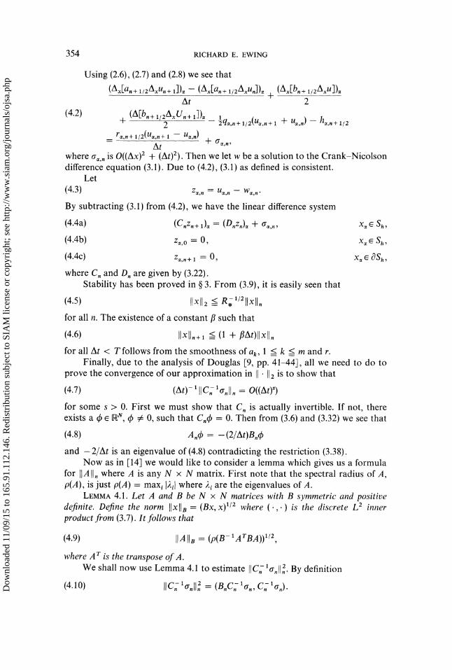
Using (2.6), (2.7) and (2.8) we see that

(Ax[a,+ 1/2Axu,+ 1]), (Ax[a,+ 1/2Axun])At 2

(A,[b. + i/2Axu])+

(4.2) (A[b, + 1/2AU,++ 2 q," +

r,,+ 1/2(b/e,n+ Ue,n)At +

where ,,, is O((Ax) + (At)2). Then we let w be a solution to the Crank-Nicolsondifference equation (3.1). Due to (4.2), (3.1) as defined is consistent.

Let(4.3) z,, u,, w,,.By subtracting (3.1) from (4.2), we have the linear difference system

(4.4a) (C,z,+ ) (D,z,) + a,,, x e Sh,

(4.4b) z,,o O, x e Sh,

(4.4c) z,,+ 0, x, e 0Sh,where C, and D, are given by (3.22).

Stability has been proved in 3. From (3.9), it is easily seen that

(4.5) I{xl12 _-< R, a/2l{xllfor all n. The existence of a constant fl such that

(4.6) Ilxll.+ (1 +for all At < T follows from the smoothness of ak, k m and r.

Finally, due to the analysis of Douglas [9, pp. 41-44], all we need to do toprove the convergence of our approximation in [[. 2 is to show that

(4.7) (At)- ’l] C- a,]], O((At))

for some s > 0. First we must show that C, is actually invertible. If not, thereexists a 4 e NN, 4 va 0, such that C,4 0. Then from (3.6) and (3.32) we see that

(4.8) A,cD (2/At)B,c

and -2 is an eigenvalue of (4.8)contradicting the restriction (3.38).Now as in [14] we would like to consider a lemma which gives us a formula

for ]]AII, where A is any N x N matrix. First note that the spectral radius of A,p(A), is just p(A) maxi ]2i1 where 2 are the eigenvalues of A.

LEMMA 4.1. Let A and B be N x N matrices with B symmetric and positivedefinite. Define the norm ]]xllB (Bx, x) 1/2 where (.,.)is the discrete L2 innerproduct from (3.7). It follows that

(4.9) IIA[I/ (p(B-1ATBA))I/2,

where A T is the transpose of A.We shall now use Lemma 4.1 to estimate [[C- la,[12,. By definition

(4.10)Dow

nloa

ded

11/0

9/15

to 1

65.9

1.11

2.14

6. R

edis

trib

utio

n su

bjec

t to

SIA

M li

cens

e or

cop

yrig

ht; s

ee h

ttp://

ww

w.s

iam

.org

/jour

nals

/ojs

a.ph

p


Since B.C is not necessarily symmetric, it would be hard to determineB.C 1112. However, since C. is symmetric, C- is symmetric,

and C[B,C[ is seen to be symmetric. Therefore, since the spectral radius of amatrix is a lower bound for any norm of the matrix [19, p. 13], we have that

(4.12)

Using separation of variables o estimate [IC B.I]., since C. B./t + ./2, wesee that

(4.13) B, XC,O (B,/At + A,/2)O.

Rearranging, we arrive at the eigenvalue problem

(4.14)

Theorem 3.1 gives the inequality from (3.36)

2 2(4.15) -A < < A2At

or

(4.16) 0 <l/At + A2/2 <= 2 <_

l/At- A1/2for the case where B, < 0 and Q, < 0. Choosing At to satisfy (3.38) we see that

At(4.17) 0 < A =<and 2 O(At). Thus we see that

(4.18) IIC-’B.II. O(At).

Then by Lemma 4.1, since C-1 is symmetric,

(4.19)

or

(4.20)

Lemma 4.1 also implies that

(4.21)

Note that

(4.22)

liB; lln p(B 1) liB/1{12.

(B,x, x)(x,x) (x,x)

(rn+ 112X x) -- E=I (a,+ 1]2(xkX (xkX) >= R,Dow

nloa

ded

11/0

9/15

to 1

65.9

1.11

2.14

6. R

edis

trib

utio

n su

bjec

t to

SIA

M li

cens

e or

cop

yrig

ht; s

ee h

ttp://

ww

w.s

iam

.org

/jour

nals

/ojs

a.ph

p


for x :/: 0. Then by the minimax principle [17, p. 181], the minimum eigenvalueof B, is bounded below by R,. Thus since the eigenvalues of B21 are reciprocalsof those of B,, we have the result

(4.23) IB-1 <= R2 .Thus combining (4.12), (4.18), (4.20) and (4.23) we have

22

(4.24)C BnC; < IIC B [[B

O((At):).

Finally, we see that by the Schwarz inequality, (4.2), and (4.24),

[C- lo’nll2n (Cff IBnCff 1o"n, O’n)

(4.25) < C21BnC; 2 Io’nlL(At)Z((Ax)2 + (At)2)2.

Thus,

(4.26) At--IC-lo’,1, O((Ax)2 + (At)2).

From (4.26), the analysis of Douglas [9, pp. 41-44] shows that

(4.27) IIz, ll, O((Ax)2 + (At)),and we have convergence in the I1" 2 of order O((Ax)2 + (At)2). We summarizethis result in the following theorem.

THEOREU 4.2. If B, < 0 and Q, < 0, under the restrictions on u, ak, bk, h,q and r indicated in (2.8), and with the restriction on At in (3.38), then the solution

of (3.1) converges to the solution of (4.1) in I1" 112. The rate of convergence is

o((Ax) + (At)2).COROLLARY 4.3. If B, > 0 and Q, > 0 the above result holds with no re-

striction on At > O.Similar results hold for other choices of B, and Q,.We have shown convergence in the discrete L2-norm. If multilinear inter-

polation is applied to the solution, the error in the integral L2-norm,

(fsf; 1/2

(4.28) IlullL= U2 dt dx

is also O((Ax)2 + (At)z) (see [7]).

5. Convergence for semilinear equations. Consider the semilinear initial-boundary value problem given by (4.1) with qu replaced by q, where

q q(xl, Xm, u, t).

For this case we need the added assumption that q is boundedly differentiable withrespect to u for all (x,..., Xm, t) in S x (0, T], -oe < u < oe. We thus assumethere are 0, and 0* satisfying

(5.1) Q, <= tgq/t?u <= Q*.Dow

nloa

ded

11/0

9/15

to 1

65.9

1.11

2.14

6. R

edis

trib

utio

n su

bjec

t to

SIA

M li

cens

e or

cop

yrig

ht; s

ee h

ttp://

ww

w.s

iam

.org

/jour

nals

/ojs

a.ph

p


As before, we shall have a consistent approximation if we define the Crank-Nicolson difference approximation to be

(/Xx[b.+ //xW.+(Ax[a,+ 1/2AxWn+ 1])e (Ax[a,+ 1/2AxWn])e +At 2

(A,[b,+ x/zAW,]), w,,+ + w,,(5.2a) + 2

q x,2

t,+ /2

r=,.+1 W,n] Xa e Sh,At

(5.2b) W=,o f, x= Sh,

(5.2C) W=,,+ g,,,+ 1, x= CSh.After a standard linearization using the mean value theorem, we see that theerror equation for the semilinear case is of the same form as that studied in 4.Just as before, we obtain the following theorem.

TnEOREM 5.1. If B, < 0 and , < O, under the restrictions on u, ak, bk, h,q and r indicated in (2.8), the added restriction that q has a bounded derivative withrespect to u for (xl ,"", x,, t) S (0, T] and < u < o, and the restrictionon At in (3.38), then the solution of the Crank-Nicolson difference approximation(5.2) converges to the solution u of (4.1), as modified, in the discrete L2-norm withdiscretization error of the form O((Ax) + (At)z).

COROLLARY 5.2. If B, > 0 and , > O, the above result holds with no re-striction on At > O.

Similar results hold for other choices of B, and Q,. Also, as in the previoussection, the above results can be extended to convergence in the integral Lz-norm (4.28) by multilinear interpolation [7].

6. Algebraic problem. Our original problem was to find a numerical approxi-mation v of the solution u to a problem like (4.1). We must now solve the algebraicproblem by showing how to determine a numerical approximation v, of thesolution w, of (5.2).

The method of solving the algebraic problem for (5.2) will be to reduce theproblem to the inversion of a certain matrix at each time level. Thus we will fixa At and consider a separate problem at each time level. If B, < 0 and Q, < 0,we have an eigenvalue problem which will force restrictions on the fixed At to bedescribed later.

In order to treat the nonlinear algebraic problem we shall use a two-leveliteration scheme. We present two schemes. The first utilizes a Picard-type outeriteration with an alternating direction inner iteration, while the second replacesthe inner iteration by an overrelaxation scheme. The first converges more rapidly,but applies to less general problems [27]. See part II of [12] for a more detailedaccount of this section.

First, let m 3, let S be a cube in 3 and consider the Crank-Nicolsondifference system (5.2) where ak a and bk b for k 1, 2, 3 with a and b con-stants. For each fixed n, we consider w,/l -= w a variable. Then for each fixedtime level, we have the problemD

ownl

oade

d 11

/09/

15 to

165

.91.

112.

146.

Red

istr

ibut

ion

subj

ect t

o SI

AM

lice

nse

or c

opyr

ight

; see

http

://w

ww

.sia

m.o

rg/jo

urna

ls/o

jsa.

php


(6.1a)

(6.1b)

where

(6.2a) Q(xe, %)

(6.2b) de,,

(Xl, X2, X3) Sh,

(X1, X2, X3) C OSh,

tn+l,

2(r.+ 1]2W)e -- 2Atq.+ 1/2(Xa, We)2a + bat

2a bat2a + bat A3we,

2(rn+ 1/2Wn)e2a + bat

and A3 is the 3-dimensional discrete Laplacian. Clearly d is independent ofw w,+ 1. We need upper and lower bounds for c3Q/cw. Using (2.8) and (5.1) weobtain

2R, + 2Q,At OQ 2R* + 2Q’At p(6.3) P 2a + bat< -w <

2a + bat

We thus consider solving the nonlinear algebraic equations (6.1) with the con-dition (6.3).

The problem (6.1)-(6.3) is now exactly in the form of the problem discussedby Douglas in [10] and in [11, pp. 59-60]. The outer iteration for the two-levelscheme is a Picard-type iteration [10], [11]. The inner, alternating direction,iteration and the parameter sequence needed to use it are given in [11]. Thefollowing theorem follows directly from the argument of [10].

THEOREM 6.1. Given p from (6.3), if p > 3z2 (the negative of the least eigen-value of the Laplace differential operator on S, the unit cube), the solution of theiteration process defined in [10], [11] converges to the solution of (6.1). The numberof calculations required to reduce the error in the solution by a factor of e is

(6.4) O((AX)- 3 log (Ax)- 1).

Now we want to consider the algebraic problem for more general operatorsfrom (4.1) as modified in {} 5. Replacing the inner iteration by a successive over-relaxation scheme, we are able to treat these more general operators. From (5.2)we consider, for S a cube in

(6.5)

(Ax[a,+l/2Axwn+l])eAt 2

(Ax[bn+l/2AxWn+l])e+

(rn+ 1/2Wn+ 1)eAt

+q XWe,n + nt- We

2t,+ 1/2 .qt_ C(xe, we,,, t,+ 1/2),

where C is independent of w,+ 1. For each n, as above, we let w,+ -= w and con-sider a separate problem. Fix n and consider

(6.6a) w Q(x,w) xe&,2

(6.6b) we ge,,+ 1, Xe - Sh’Dow

nloa

ded

11/0

9/15

to 1

65.9

1.11

2.14

6. R

edis

trib

utio

n su

bjec

t to

SIA

M li

cens

e or

cop

yrig

ht; s

ee h

ttp://

ww

w.s

iam

.org

/jour

nals

/ojs

a.ph

p


where

(6.7a) Q(x,, w) (r,,+ 1/2w)/At + q,,+ 1/2(Xa, Wa) + Co,n + 1,

(6.7b) C,+ 2

Clearly C is independent of w w/ . Thus from (2.8) and (5.1) we see that

R, t?Q R* Q,(6.8) P + O, < cw < At + P"

As before we consider a two-level iteration. The outer iteration is as before,while the inner iteration is a successive overrelaxation iteration [15], [273, [29].The outer iteration is actually of the form

{ IAx[an+ /2Ax] Ax[bn+ l/2Ax] A]w(k+ 1)}(6.9a) At +2

Q(x, w) Aw + , x S,

(6.9b) wk + 1) g, x e t?Sh,

where a is the residual at the end of the inner iteration. As in [10] it is not neces-sary that the linear equations be solved exactly.

Consider the convergence of w(k) to w. Let

(6.10) z)= w+l)_ w), k 1,2,....

Using (6.10) and the mean value theorem,

{ IAx[an+ I/2Ax] Ax[bn+ l/2Ax] Alztk’}At +2

(6.1 la)Q--wI,, w,*)z - Az - + - Xa Sh

(6.11 b) zk) O, x e C3Sh.

Separating variables, we have the eigenvalue problem

(6.12a) Etk vFdp, x, e Sh,

(6.12b) ck O, x e CSh,

where

(6.13a)

(6.13b)

(E4), (Ow(X,,W*)4)[Ax[a,.+__x_/zA,](F4)k At + Ax[b, + 1/2Ax]

Clearly E and F are symmetric matrices. We can define a consistent ordering andobtain an N x N matrix representation for F which is diagonally dominantD

ownl

oade

d 11

/09/

15 to

165

.91.

112.

146.

Red

istr

ibut

ion

subj

ect t

o SI

AM

lice

nse

or c

opyr

ight

; see

http

://w

ww

.sia

m.o

rg/jo

urna

ls/o

jsa.

php


[30], [32] and positive definite by restricting

(6.14) At < 2A,/[B,[if B, < 0. No such restriction is necessary if B, >__ 0.

Thus from 4, pp. 37-41], we know that (6.12) has a complete set of eigen-vectors which are orthogonal with respect to the inner product (FqS, q) as in (3.11),and we can apply the Courant minimax principle as before. As in part II of 12]we can get bounds on the eigenvalues of (6.12) by considering the eigenvalueproblem

zXcb Acb x e Sh,(6.15a) IQ AI 2 + 2

k=l

(6.15b) O, x Sh.As in 3, by rearranging the above eigenvalue problem and applying the

Courant minimax principle and a special case of the minimax theorem [17,p. 181], we have for a cube

(6.16) max Ivl < IQ AIi=1 N ([A,/At + B,/2](m 6)rt2 + A)’

where [Q A] is given by

(6.17) IQ- A] max {]Q, A], ]Q* A]}.

Thus from (6.11), (6.12) and (6.16), we see that

(6.18)

[Q A[ztk)ll2 <= ([A,/At + B,/2](m- 6)rt2 + A)

-+ (m- 6)7t2 + A-1

(() 2 + (- ) 2).

Thus letting

(6.19) p([A,/At + B,/2](m- 6)rc2 + A)

and requiring sufficient iterations on the inner iteration so that

(6.20) a{) [A,/At + B,/2] (m 1)2 pk+2 < l+p

we see that

(6.21) 2(k) [2 < /9 2(k- 1)[2 -}" Ok"

For convergence, it is necessary that

(6.22) IQ-AI < -+ mrc2 +A.

Dow

nloa

ded

11/0

9/15

to 1

65.9

1.11

2.14

6. R

edis

trib

utio

n su

bjec

t to

SIA

M li

cens

e or

cop

yrig

ht; s

ee h

ttp://

ww

w.s

iam

.org

/jour

nals

/ojs

a.ph

p


One sufficient condition is that

R, A, _,)(6.23) p - + Q, > -- + mzc2

Since R, > 0, this restriction can be met by taking At sufficiently small. Wenote that (6.23) will hold with no restriction on At if Q, >__ 0 and B, >__ 0.

Now consider the inner, SOR iteration. Each inner iteration consists ofapproximating the solution of an elliptic difference equation of the form (6.9) byan SOR method. After defining a consistent ordering, as in [30, p. 108], we canobtain a system of N linear equations in N unknowns where for i, j 1, 2, ..., Nwe have a system of the form

N

(6.24) ai,jv + dj O.j=l

As before, we see that C (ai,j) is positive definite under the restriction

(6.25) At < 2A,/[B,]with B, < 0 and with no restriction on At if B, __> 0.

Now we define the following iterative scheme for the elements of C. Usingsquare brackets to distinguish an index of the inner iteration from the outeriteration we have

(6.26) ,,k + 1] (co 1)vlk]j=l j=i+l

k_>_0, i= 1,2,...,N,

where vl1 is arbitrary, l, 2,..., N, and where

--ai,j/ai,i,(6.27) bi4= O,

and

:/: j,

i=j,

Equation (6.26) may be written in the form

(6.29)[klwhere vkl- (vkl, vtkl2 VN ), f- (fl rE, fN), f is fixed, and L denotes a

linear operator. Here co denotes the relaxation factor. Young 32] defines anoptimal relaxation factor, cob, in terms of the spectral norm/ of B (bi4) from(6.27). As shown in 32], it is better to overestimate cob. By restricting At as in(6.25) if necessary, we can obtain, as in I31], a rigorous upper bound for fi andthus a nontrivial upper bound coo for cob. With this upper bound coo as a re-laxation factor, the rate of convergence R(Lo will be of the same order as R(Lo).

As in 30], 32], we see that the number of cycles of SOR iteration sweepsrequired for each outer iteration is O((Ax)-1). Thus since the number of cal-culations per sweep is O((Ax)-m), we have the following result.

(6.28) C di/ai,i 1,2, N

Dow

nloa

ded

11/0

9/15

to 1

65.9

1.11

2.14

6. R

edis

trib

utio

n su

bjec

t to

SIA

M li

cens

e or

cop

yrig

ht; s

ee h

ttp://

ww

w.s

iam

.org

/jour

nals

/ojs

a.ph

p


THEOREM 6.2. By restricting At to satisfy (6.23) and (6.25) when B, < 0 andQ, < 0 and if (6.20) is satisfied, then the solution of the iteration process definedby (6.9) and (6.26)-(6.28) converges to the solution of (6.6). The number of cal-culations required to reduce the error in the solution by a factor of e is

(6.30) O((Ax)-t,, + 1)).COROLLARY 6.3. The above result holds with no restriction on At if B, > 0

and Q, > O.Similar results hold for other choices of B, and Q,. We note that since the

SOR iteration procedure does not require a rectangular region as does thealternating direction method, the region could be generalized to the arbitraryregion described in 2 as in [30].

REFERENCES

[1] G. BARENBLATT, I. ZHELTOV AND I. KOCHINA, Basic concepts in the theory ofseepage ofhomogeneousliquids in fissured rocks, J. Appl. Math. Mech., 24 (1960), pp. 1286-1303.

[2] P. J. CUES AND M. E. GURTIN, On a theory of heat conduction involving two temperatures, Z.Angew. Math. Phys., 19 (1968), pp. 614-627.

[3] B. D. COLEMAN AND W. NOEL, An approximation theorem for functionals, with applications to

continuum mechanics, Arch. Rational Mech. Anal., 6 (1960), pp. 355-370.[4] R. COURANT AND D. HILBERT, Methods of Mathematical Physics, vol. 1, Interscience, New

York, 1953.[5] J. CRANK AND R. NICOLSON, A practical methodfor numerical evaluation of solutions ofpartial

differential equations of heat-conduction type, Proc. Cambridge Philos. Soc., 43 (1947),pp. 50-67.

[6] P. L. DAVIS, A quasilinear parabolic and a related third order problem, J. Math. Anal. Appl., 40(1972), pp. 327-335.

[7] J. DOUGLAS, JR., On the relation between stability and convergence in the numerical solution oflinear parabolic and hyperbolic differential equations, J. Soc. Indust. Appl. Math., 4 (1956),pp. 20-37.

[8] -, The application of stability analysis in the numerical solution of quasi-linear parabolic

differential equations, Trans. Amer. Math. Soc., 89 (1958), pp. 484-518.[9] ., A survey of numerical methods for parabolic differential equations, Advances in Com-

puters, vol. II, Academic Press, New York, 1961.[10] -, Alternating direction iteration for mildly nonlinear elliptic difference equations, Numer.

Math., 3 (1961), pp. 92-98.[11], Alternating direction methods for three space variables, Ibid., 4 (1962), pp. 41-63.[12] R. E. EWlNt3, The numerical approximation of certain parabolic equations backward in time via

Sobolev equations, Doctoral thesis, Univ. of Texas at Austin, Austin, 1974.[13] , The approximation of certain parabolic equations backward in time by Sobolev equations,

SIAM J. Math. Anal., 6 (1975), pp. 283-294.[14] W. H. FORD, Numerical solution of pseudo-parabolic partial differential equations, Doctoral

thesis, Univ. of Illinois at Urbana-Champaign, Urbana, 1972.[15] S. P. FRANKEL, Convergence rates of iterative treatments ofpartial differential equations, Math.

Tables Aids. Comput., 4 (1950), pp. 65-75.[16] H. GAJEWSKI AND K. ZACHARIAS, Ztlr Starken Konvergenz des Galerkinverfahrens bei einer

Klasse Pseudoparabolischer Partialler Differentialgleichungen, Math. Nach., 47 (1970),pp. 365-376.

[17] P. R. HALMOS, Finite Dimensional Vector Spaces, Van Nostrand, Princeton, N.J., 1958.[18] R. HUILGOL, A second orderfluid of the differential type, Internat. J. Nonlinear Mech., 3 (1968),

pp. 471-482.[19] A. R. MITCHELL, Computational Methods in Partial Differential Equations, John Wiley, London,

1969.Dow

nloa

ded

11/0

9/15

to 1

65.9

1.11

2.14

6. R

edis

trib

utio

n su

bjec

t to

SIA

M li

cens

e or

cop

yrig

ht; s

ee h

ttp://

ww

w.s

iam

.org

/jour

nals

/ojs

a.ph

p


[20] W. E. MILNE, Numerical Solutions of Differential Equations, John Wiley, New York, 1953.[21] R. E. SHOWALTER, Weak solutions of nonlinear evolution equations of Sobolev-Galpern type, J.

Differential Equations, 11 (1972), pp. 252-265.[22] -, Partial differential equations of Sobolev-Galpern type, Pacific J. Math., 31 (1969), pp.

787-793.[23] --., Thefinal-value problem for evolution equations, J. Math. Anal. Appl., to appear.[24] R. E. SHOWALTER AND T. W. TING, Pseudo-parabolic partial differential equations, SIAM J.

Math. Anal., (1970), pp. 1-26.[25] D. TAYLOR, Research on Consolidation of Clays, Massachusetts Institute of Technology Press,

Cambridge, Mass., 1952.[26] T. W. TING, Certain non-steady flows of second order fluids, Arch. Rational Mech. Anal., 14

(1963), pp. 1-26.[27] R. S. VARGA, Matrix Iterative Analysis, Prentice-Hall, Englewood Cliffs, N.J., 1962.[28] K. YOSIDA, Functional Analysis, Die Grundlehren der Mathematischen Wissenschaften in Ein-

zeldarstellungen, 123, Springer-Verlag, Berlin-Heidelberg-New York, 1965.[29] DAWD M. YOUNG, Iterative methodsfor solvingpartial difference equations ofelliptic type, Doctoral

thesis, Harvard Univ., Cambridge, Mass., 1950.[30] ---, Iterative methods for solving partial difference equations of elliptic type, Trans. Amer.

Math. Soc., 76 (1954), pp. 92-111.[31] --, A bound for the optimum relaxation factor for the successive overrelaxation method,

Numer. Math., 16 (1971 ), pp. 408-413.[32] DAVID M. YOUNG AND ROBERT T. GREGORY, A Survey of Numerical Mathematics, vol. II,

Addison-Wesley, Reading, Mass., 1973.

Dow

nloa

ded

11/0

9/15

to 1

65.9

1.11

2.14

6. R

edis

trib

utio

n su

bjec

t to

SIA

M li

cens

e or

cop

yrig

ht; s

ee h

ttp://

ww

w.s

iam

.org

/jour

nals

/ojs

a.ph

p

numerical solution of sobolev partial differential...

Documents