numerical simulation of wind load on roof mounted solar panels · numerical simulation of wind load...

University of WindsorScholarship at UWindsor

Electronic Theses and Dissertations

2012

Numerical Simulation of Wind Load on RoofMounted Solar PanelsYuanming YuUniversity of Windsor

Follow this and additional works at: http://scholar.uwindsor.ca/etd

This online database contains the full-text of PhD dissertations and Masters’ theses of University of Windsor students from 1954 forward. Thesedocuments are made available for personal study and research purposes only, in accordance with the Canadian Copyright Act and the CreativeCommons license—CC BY-NC-ND (Attribution, Non-Commercial, No Derivative Works). Under this license, works must always be attributed to thecopyright holder (original author), cannot be used for any commercial purposes, and may not be altered. Any other use would require the permission ofthe copyright holder. Students may inquire about withdrawing their dissertation and/or thesis from this database. For additional inquiries, pleasecontact the repository administrator via email ([email protected]) or by telephone at 519-253-3000ext. 3208.

Recommended CitationYu, Yuanming, "Numerical Simulation of Wind Load on Roof Mounted Solar Panels" (2012). Electronic Theses and Dissertations. Paper218.

http://scholar.uwindsor.ca?utm_source=scholar.uwindsor.ca%2Fetd%2F218&utm_medium=PDF&utm_campaign=PDFCoverPages

http://scholar.uwindsor.ca/etd?utm_source=scholar.uwindsor.ca%2Fetd%2F218&utm_medium=PDF&utm_campaign=PDFCoverPages

http://scholar.uwindsor.ca/etd?utm_source=scholar.uwindsor.ca%2Fetd%2F218&utm_medium=PDF&utm_campaign=PDFCoverPages

http://scholar.uwindsor.ca/etd/218?utm_source=scholar.uwindsor.ca%2Fetd%2F218&utm_medium=PDF&utm_campaign=PDFCoverPages

mailto:[email protected]

i

Numerical Simulation of Wind Load on Roof Mounted Solar Panels

by

Yuanming Yu

A Thesis

Submitted to the Faculty of Graduate Studies through the Department of Mechanical,

Automotive and Materials Engineering in Partial Fulfillment of the Requirements for the

Degree of Master of Applied Science at the University of Windsor

Windsor, Ontario, Canada

2012

©2012 Yuanming Yu

ii

Numerical Simulation of Wind Load on Roof Mounted Solar Panels

by

Yuanming Yu

Approved By:

Dr. Shaohong Cheng, External Department Reader

Department of Civil and Environmental Engineering

Dr. David Ting, Department Reader

Department of Mechanical, Automotive and Materials Engineering

Dr. Ronald Barron, Co-Advisor

Department of Mathematics and Statistics and Department of Mechanical,

Automotive and Materials Engineering

Dr. Ram Balachandar, Co-Advisor

Department of Civil and Environmental Engineering and Department of Mechanical,

Automotive and Materials Engineering

Dr. N. Zamani, Committee Chair

Department of Mechanical, Automotive and Materials Engineering

iii

AUTHOR’S DECLARATION OF ORIGINALITY

I hereby certify that I am the sole author of this thesis and that no part of this

thesis has been published or submitted for publication.

I certify that, to the best of my knowledge, my thesis does not infringe upon

anyone’s copyright nor violate any proprietary rights and that any ideas, techniques,

quotations, or any other material from the work of other people included in my thesis,

published or otherwise, are fully acknowledged in accordance with the standard

referencing practices. Furthermore, to the extent that I have included copyrighted material

that surpasses the bounds of fair dealing within the meaning of the Canada Copyright

Act, I certify that I have obtained a written permission from the copyright owner(s) to

include such material(s) in my thesis and have included copies of such copyright

clearances to my appendix.

I declare that this is a true copy of my thesis, including any final revisions, as

approved by my thesis committee and the Graduate Studies office, and that this thesis has

not been submitted for a higher degree to any other University or Institution.

iv

ACKNOWLEDGEMENTS

I would never have been able to finish my thesis without the guidance of my

committee members, help from my colleagues, and supports from my family and wife.

Dr. Ting and Dr. Cheng presented a lot of interesting questions in the proposal

meeting, which pushed me to think deeper and wider. Many colleagues, especially Kohei,

gave me much help during my research period. I really appreciate their kind help.

I would like to take this opportunity to express my deepest gratitude to my

advisors, Dr. Barron and Dr. Balachandar for their great guidance, caring, patience and

providing me with an excellent research atmosphere. I also really want to thank the

Natural Sciences and Engineering Research Council (NSERC) and Polar Racking Inc. for

providing an NSERC Industrial Postgraduate Scholarship to carry out my research. I also

offer my thanks to the University of Windsor for providing me with Graduate

Assistantship opportunities during my graduate study period.

v

ABSTRACT

Seven RANS models (Spalart-Allmaras, k-ε, k-ω and their variants, Reynolds Stress

Model (RSM)), DES-SST and LES model have been used to predict the pressure

coefficient (Cp) distribution on a cube and the Cp difference of a canopy in an

atmospheric boundary layer flow. The simulation results show that k-ω-SST gives the

best prediction in both cases. The RSM also accurately predicts the Cp in the cube case.

The k-ω-SST and DES-SST models have been used to simulate the wind load on flat roof

mounted solar panels under similar flow conditions with different wind attack angles. The

simulation results demonstrate that both k-ω-SST and DES-SST give good prediction of

the drag force at all wind attack angles and reasonably good prediction of the lift force at

most wind attack angles. The k-ω-SST model has also been used to investigate the

change of wind load on solar panels with three different configurations.

vi

TABLE OF CONTENTS

Author’s Declaration of Originality…………………………………………..…..……..iii

Acknowledgements…………………………………………………………………..…..iv

Abstract…………………………………………………………………………………...v

List of Tables…………………………………………………..…………………………x

List of Figures…………………………………………………………………………….xi

Nomenclature…………………………………………………………………………….xv

CHAPTER 1

Introduction…………………………………………………………….………………….1

1.1 Methods to Determine Wind Loads on Solar Panels……...………………..................1

1.2 Flow around a Cubic Shaped Building……………………………………………….1

1.3 Previous Predictions of Pressure Distribution on a Cube Building…………………...2

1.4 Prediction of Wind Load on a Roof Mounted Solar Panel by Wind Tunnel Test…….3

1.5 Prediction of Wind Load on a Roof Mounted Solar Panel by CFD…………………..4

1.6 Conclusions…………………………………………………………………………....4

1.7 Objectives of the Thesis…………………………………………………………….…5

CHAPTER 2

Pressure Coefficient on a Cube in an Atmospheric Boundary Layer.........……………....6

2.1 Flow Problem Description…………………………………………………..………..6

2.2 Governing Equations………………………………………………………………….7

2.2.1 Reynolds Averaged Navier-Stokes (RANS)………………………….…….8

vii

2.2.2 Large Eddy Simulation (LES)……………………………………..…...…..8

2.2.3 Detached Eddy Simulation (DES)……………………………….…..……..9

2.3 Near-Wall Treatment………………………………………………..………...…..…10

2.4 Computational Domain and Test Cases…………………………………….….…….10

2.5 Boundary Conditions……………………………………………………….….…….12

2.6 Mesh Topology…………………………………………………………….…….…..13

2.7 Numerical Setup………………………………………………………………....…..14

2.8 Simulation Results……………………………………………………………..…….14

2.8.1 Cp Distribution in Vertical Symmetry Plane of the Cube……….…..….….14

2.8.2 Flow Pattern around the Cube………………………………………..…….18

2.8.3 Flow Recirculation Length……………………………………….….….…23

2.9 Discussion and Conclusions…………………………………………………..…..…23

CHAPTER 3

Wind Load on a Free Standing Roof in an Atmospheric Boundary Layer……………....25

3.1 Flow Problem Description……………………………………………………….......25

3.2 Governing Equations…………………………………………………………..….....27

3.3 Computational Domain…………………………………………………….….….....27

3.4 Boundary Conditions…………………………………………….………….…..…..28

3.5 Mesh Topology………………………………………………………..….……...….28

3.6 Numerical Setup……………………………………………………….…….…..….28

3.7 Simulation Results…………………………………………………….….…….…...29

viii

3.7.1 Wind Load on the Canopy Roof………………………………….…...…...29

3.7.2 Velocity Field around the Canopy……………………………….…..….....36

3.8 Discussion and Conclusions………………………………………………….….......38

CHAPTER 4

Mean and Peak Wind Load on Flat Roof Mounted Solar Panels in an Atmospheric

Boundary Layer (Basic Case)…………………………………………………......…......40

4.1 Flow Problem Description………………………………………………….…..…....40

4.2 Governing Equations…………………………………………….…….….....….…...42

4.3 Computational Domain ……………………………………………….….…..….…..43

4.4 Boundary Conditions…………………………………………………….…...….…..44

4.5 Mesh Topology……………………………………………………….…….....……..44

4.6 Numerical Setup……………………………………………………………….……..45

4.7 Simulation Results………………………………………………………….………..45

4.7.1 Area-averaged Pressure Coefficient Difference for the Solar Panels….…..45

4.7.2 Pressure Coefficient Difference for the Wind Deflector……………….….48

4.7.3 Drag Coefficient for the Solar Panel Assembly using k-ω-SST………..….50

4.7.4 Lift Coefficient for the Solar Panel Assembly using k-ω-SST…………….51

4.7.5 Mean Drag Coefficient for the Solar Panel Assembly using DES-SST…...51

4.7.6 Mean Lift Coefficient for the Solar Panel Assembly using DES-SST….....52

4.7.7 Peak Drag Coefficient for the Solar Panel Assembly using DES-SST……53

4.7.8 Peak Lift Coefficient for the Solar Panel Assembly using DES-SST……..54

ix

4.8 Discussion and Conclusions………………………………………………….….…55

CHAPTER 5

Mean Wind Load on Roof Mounted Solar Panel Arrays in an Atmospheric Boundary

Layer (Other Configurations)………………………………………………….….…….56

5.1 Simulation Results……………………………………………………….………….56

5.1.1 Drag Coefficient for the Solar Panel Assembly…………………..………56

5.1.2 Lift Coefficient for the Solar Panel Assembly……………….….………..58

5.2 Conclusions………………………………………………………….……….……..60

CHAPTER 6

Conclusions and Future Work……………………………………………….………….62

6.1 Conclusions……………………………………………………………..…………..62

6.2 Future Work………………………………………………………..………….……64

APPENDIX A

Turbulence Models……………………………………………………………………..65

APPENDIX B

Near-Wall Treatment…………………………………………………………………...76

References………………………………………………………………………..….….79

Vita Auctoris……………………………………………………………………………83

x

LIST OF TABLES

Table 2.1 Extent of computational domain (h: cube height)…………………………....10

Table 2.2 Flow recirculation length in the wake region (h: cube height)……………….23

xi

LIST OF FIGURES

Fig. 2-1 Comparison of experimental results and numerical prediction (k-ω-SST) at cube

location, without presence of the cube, (a) velocity profile; (b) turbulent kinetic energy...7

Fig. 2-2 Computational domain II (horizontal layout, not to scale)…………………..…11

Fig. 2.3 Computational domain II (cross-sectional layout, not to scale)……………...…11

Fig.2-4 Effect of computational domain size on Cp distribution……………………...…12

Fig 2-5 Tetrahedral mesh around the cube………………………………………………13

Fig. 2-6 Cp distribution at vertical symmetry plane from (a) k-ω standard and k-ω-SST

models; (b) Reynolds Stress Model (RSM) and Spalart-Allmaras (SA) model………....16

Fig. 2-7 Cp distribution at vertical symmetry plane from (a) k-ε standard, k-ε RNG and k-ε

Realizable models; (b) DES–SST and LES (dynamic Smagorinsky) models……….......17

Fig. 2-8 Streamtraces predicted by Spalart-Allmaras model, (a) vertical symmetry plane;

(b) horizontal plane at 0.125h…………………………………………………….….…..18

Fig. 2-9 Streamtraces predicted by k-ε standard model, (a) vertical symmetry plane;

(b) horizontal plane at 0.125h………………………………………………….…….…..19

Fig. 2-10 Streamtraces predicted by k-ε RNG model, (a) vertical symmetry plane; (b)

horizontal plane at 0.125h……………………………………………………………......19

Fig. 2-11 Streamtraces predicted by k-ε Realizable model, (a) vertical symmetry plane;

(b) horizontal plane at 0.125h………………………………………………….………...20

Fig. 2-12 Streamtraces predicted by k-ω standard model, (a) vertical symmetry plane;

(b) horizontal plane at 0.125h……………………………………………………….…...20

Fig. 2-13 Streamtraces predicted by k-ω-SST model, (a) vertical symmetry plane; (b)

horizontal plane at 0.125h…………………………………………….……………….....21

Fig. 2-14 Streamtraces predicted by Reynolds Stress Model, (a) vertical symmetry plane;

(b) horizontal plane at 0.125h……………………………..…………..............................21

xii

Fig. 2-15 Streamtraces predicted by DES-SST model, (a) vertical symmetry plane; (b)

horizontal plane at 0.125h……………………………………………………….….…...22

Fig. 2-16 Streamtraces predicted by LES (dynamic Smagorinsky), (a) vertical symmetry

plane; (b) horizontal plane at 0.125h……………………………………...…….….…....22

Fig. 3-1 Geometry of the canopy with 0o wind attack angle……………………….…....26

Fig. 3-2 Velocity profile near canopy location……………………………………...…...26

Fig. 3-3 Turbulence intensity profile in streamwise direction near canopy location…....26

Fig. 3-4 Computational domain (horizontal layout, not to scale)………………………..27

Fig. 3-5 Tetrahedral mesh around the canopy in cross-section layout……………...…...28

Fig. 3-6 ∆Cp at different wind attack angles predicted by RANS models (coarse mesh near the canopy)………………………………………..…………………………....…...30 Fig. 3-7 ∆Cp at different wind attack angles by RANS models (fine mesh near the canopy)

………………………………………………………………..……………….…….…....31

Fig. 3-8 ∆Cp at different wind attack angles by RSM, k-ε standard, RNG, Realizable

(coarse mesh near the canopy)………………………………………...…….….….….....32

Fig. 3-9 ∆Cp at different wind attack angles by RSM, k-ε standard, RNG, Realizable (fine

mesh near the canopy)……………………………………………….………….….…....33

Fig. 3-10 ∆Cp at different wind attack angles by DES-SST and LES (coarse mesh near the canopy)……………………………………….…………………………….…….…..….34 Fig. 3-11 Mean drag coefficient at different wind attack angles by DES-SST and LES

(coarse mesh near the canopy)……………………………………………………...…....35

Fig. 3-12 Mean lift coefficient at different wind attack angles by DES-SST and LES

(coarse mesh near the canopy)……………………….……………………………..…....35

Fig. 3-13 Peak drag coefficient at different wind attack angles by DES-SST and LES

(coarse mesh near the canopy)……………………………….……………..…………....36

xiii

Fig. 3-14 Peak lift coefficient at different wind attack angles by DES-SST and LES

(coarse mesh near the canopy)………………………………….………………….….…36

Fig. 3-15 Flow velocity vectors near the canopy at wind attack angle of 0o, predicted by

k-ω-SST…………………………………………………………………..….………..…37

Fig. 3-16 Pressure coefficient contours for top of plate e (left) and plate b (right)……...38

Fig. 3-17 Pressure coefficient contours for bottom of plate e (left) and plate b (right)….39

Fig. 4-1 Simulated solar panel layout on a square roof………………………………….41

Fig. 4-2 Velocity profile at location of the building, without presence of the building....42

Fig. 4-3 Turbulence intensity in streamwise direction at building location, without

presence of the building……………………………………………………………….....42

Fig. 4-4 Computational domain horizontal plan layout (not to scale)…………………...43

Fig. 4-5 Computational domain vertical plan layout (not to scale)……………………...44

Fig. 4-6 Vertical cross-sectional view of the fine mesh (2mm) around the corner solar

panel array………………………………………………………………………..….…..44

Fig. 4-7 Cp difference on the solar panel predicted by k-ω-SST……………………..….46

Fig. 4-8 Velocity vectors near the solar panels at 360o wind attack angle………………47

Fig. 4-9 Velocity vectors near the solar panels at 320o wind attack angle………………47

Fig. 4-10 Velocity vectors near the solar panels at 270o wind attack angle……………..48

Fig. 4-11 Velocity vectors near the solar panels at 180o wind attack angle……………..48

Fig. 4-12 Cp difference on the wind deflector predicted by k-ω-SST……………….…...49

Fig. 4-13 Drag coefficient for the solar panel assembly predicted by k-ω-SST……..…..50

Fig. 4-14 Lift coefficient for the solar panel assembly predicted by k-ω-SST……….….51

xiv

Fig. 4-15 Mean drag coefficient for the solar panel assembly predicted by DES-SST (with

coarse mesh)………………………………………………………………………....…..52

Fig. 4-16 Mean lift coefficient for the solar panel assembly predicted by DES (with

coarse mesh)……………………………………………………………………………..53

Fig. 4-17 Peak drag coefficient for the solar panel assembly predicted by DES (with

coarse mesh)………………………………………………………………….…..….…..54

Fig. 4-18 Peak lift coefficient for the solar panel assembly predicted by DES (with coarse

mesh)………………………………………………………………………………..…...54

Fig. 5-1 Drag coefficient for three configurations of the solar panel assembly…..….….57

Fig. 5-2 Velocity vector field at wind attack angle of 330o for vertical spacing of 6 inches

off the roof…………………………………………………………………………..…...58

Fig. 5-3 Velocity vector field at wind attack angle of 330o for vertical spacing at same

height as the parapet…………………………………………………………..….…..….58

Fig. 5-4 Lift coefficient for three configurations of the solar panel assembly……….….60

Fig. 5-5 Velocity vectors at wind attack angle of 210o for vertical spacing at the same

height as the parapet……………………………………………………………………..60

xv

NOMENCLATURE

𝐶𝜇 Constant, used to calculate dynamic turbulent viscosity

∆𝐶𝑝 Pressure coefficient difference

CD Mean drag coefficient

CL Mean lift coefficient

h Height of the cube or building

k Turbulent kinetic energy

kp Turbulent kinetic energy at node P

𝑙 The length scale of flow structure

𝑝 Static pressure

𝑝0 Reference pressure at ambient region

𝑝𝑇 Area averaged pressure at top surface

𝑝𝐵 Area averaged pressure at bottom surface

𝑇𝑖 Turbulent intensity

U Velocity magnitude

𝑈𝑝 Mean velocity in the near wall node P

𝑈∗ Nondimensional velocity

uref Reference velocity in streamwise direction

𝑢𝑖 Velocity components, where i = 1, 2, 3 indicates x, y, z directions

𝑢𝑧 Streamline velocity (x direction) at z coordinate location

𝑢𝑖′ Velocity fluctuation, where i = 1, 2, 3 indicates x, y, z directions

𝑥𝑖 Coordinates, where i = 1, 2, 3 indicates x, y, z directions

𝑦∗ Nondimensional distance from wall

yp Distance from wall to node P

xvi

𝑦+ Nondimensional distance

z z coordinate

𝑧𝑟𝑒𝑓 Reference height

𝛼 Exponent of power law or wind attack angle

𝛿𝑖𝑗 Kronecker delta (𝛿𝑖𝑗 = 1 𝑖𝑓 𝑖 = 𝑗 𝑎𝑛𝑑 𝛿𝑖𝑗 = 0 𝑖𝑓 𝑖 ≠ 𝑗)

𝜏𝑖𝑗 Reynolds stress tensor

𝜏𝑤 Wall shear stress

𝜌 Density of the fluid

𝜇 Dynamic viscosity of fluid

𝜇𝑡 Turbulent viscosity of the fluid

𝑣� Modified kinematic viscosity (Spalart-Allmaras)

𝜎𝑣� Constant = 2/3 (Spalart-Allmaras)

𝐶𝑏1 Constant = 0.1355 (Spalart-Allmaras)

𝐶𝑏2 Constant = 0.622 (Spalart-Allmaras)

𝐶𝑣1 Constant = 7.1 (Spalart-Allmaras)

Cw1 Constant for dissipation term (Spalart-Allmaras)

𝑓w Wall damping function, used in dissipation term (Spalart-Allmaras)

Ω� Component of the production term (Spalart-Allmaras)

Ω Magnitude of the vorticity (Spalart-Allmaras)

Ω𝑖𝑗 Rate-of-rotation tensor (Spalart-Allmaras)

𝑓𝑣1 Viscosity damping function, used to calculate 𝜇𝑡 (Spalart-Allmaras)

𝑓𝑣2 Wall damping function, used to calculate Ω� (Spalart-Allmaras)

𝛿𝑖𝑗 Kronecker delta (Spalart-Allmaras)

𝜅 von Karman constant = 0.4187 (Spalart-Allmaras)

xvii

𝜒 Ratio of modified kinematic viscosity to viscosity (Spalart-Allmaras)

𝐺𝑘 Production term of k equation (k-ε standard, RNG, Realizable, k-ω standard)

𝑌𝑘 Dissipation term of k equation (k-ε standard)

ε Turbulent energy dissipation rate per unit mass (k-ε)

𝐺𝜀 Production term of ε equation (k-ε standard)

𝑌𝜀 Dissipation term of ε equation (k-ε standard)

𝜎𝑘 Constant = 1.0, used in diffusion term in k equation (k-ε standard)

𝜎𝜀 Constant = 1.3, used in diffusion term in ε equation (k-ε standard)

S Modulus of mean rate-of-strain tensor (k-ε standard)

𝑆𝑖𝑗 Strain tensor (k-ε standard)

𝐶1𝜀 Constant, used in production term in ε equation (k-ε standard)

𝐶2𝜀 Constant, used in dissipation term in ε equation (k-ε standard)

𝛼𝑘 Constant = 1.39, used for diffusion term in equation of k (RNG)

𝜇𝑒𝑓𝑓 Effective viscosity (RNG)

𝛼𝜀 Constant = 1.39, used for diffusion term in equation of ε (RNG)

𝐶1𝜀 Constant for production term in equation of ε (RNG)

𝐶2𝜀∗ Constant for dissipation term in equation of ε (RNG)

𝐶2𝜀 Constant, used to find 𝐶2𝜀∗ (RNG)

𝐶𝜇 Constant = 0.0845, used in turbulent viscosity (RNG)

𝜂 Constant obtained from modulus of mean rate-of-strain tensor (RNG)

𝜂0 Constant = 4.377, used to find 𝐶2𝜀∗ (RNG)

𝛽 Constant = 0.012, used to find 𝐶2𝜀∗ (RNG)

𝐶𝜇 Constant for turbulent viscosity (Realizable)

𝑈∗ Constant, used to calculate 𝐶𝜇 (Realizable)

xviii

Ω𝑖𝑗 Mean rate-of-rotation tensor (Realizable)

ωk Angular velocity (Realizable)

𝜀𝑖𝑗𝑘 Permutation tensor (Realizable)

A0 Model constant = 4.04, used to find value of 𝐶𝜇 (Realizable)

𝐴𝑠 Model variable constant, used to find value of 𝐶𝜇 (Realizable)

𝐶1 Constant, used in production term of 𝜀 equation (Realizable)

𝐶2 Constant = 1.9, used in dissipation term of 𝜀 equation (Realizable)

𝜎𝑘 Constant = 1.0, used in diffusion term of k equation, (Realizable)

𝜎𝜀 Constant = 1.2, used in diffusion term of ε equation (Realizable)

𝜙 Constant angle, used to find 𝐴𝑠 (Realizable)

𝑊 Constant, related to strain tensor, used to find 𝜙 (Realizable)

�̃� Constant used to find W (Realizable)

𝜔 Specific dissipation rate

Γ𝑘 Constant of diffusion term of k equation (k-ω standard)

Γ𝜔 Constant in diffusion term of ω equation (k-ω standard)

𝜎𝑘 Constant = 2.0, used to find Γ𝑘, for incompressible and high Re flow (k-ω standard)

𝜎𝜔 Constant = 2.0, used to find Γ𝜔 , for incompressible and high Re flow (k-ω standard)

𝛼∗ Constant used to find 𝜇𝑡, equals 1 in high Re flow (k-ω standard)

𝛼∞∗ Constant used to find 𝛼∗, equals 1 for high Re flow (k-ω standard)

𝑅𝑒𝑡 Constant used to find 𝛼∗ (k-ω standard)

𝑅𝑘 Constant = 6.0, used to find 𝛼∗ for low Re flow (k-ω standard)

𝛼0∗ Constant = 𝛽𝑖3

, used to find 𝛼∗ for low Re flow (k-ω standard)

𝛽𝑖 Constant = 0.072 (k-ω standard)

xix

𝐺𝜔 Production term of ω equation (k-ω standard)

𝛼 Constant used in production term of ω equation, equals 1 for high Re flow (k-ω standard)

𝛼∞ Constant used to find 𝛼, equals 1 for high Re flow (k-ω standard)

𝑓𝛽∗ Constant, used to find dissipation term of k equation (k-ω standard)

𝑥𝑘 Constant, used to find 𝑓𝛽∗ (k-ω standard)

𝛽∗ Constant used to find dissipation term of k equation (k-ω standard)

𝛽∞∗ Constant = 0.09, used to find 𝛽∗ (k-ω standard)

𝑌𝜔 Dissipation term of the ω equation term (k-ω standard)

𝑓𝛽 Constant, used to find 𝑌𝜔 (k-ω standard)

𝑥𝜔 Constant, used to find 𝑓𝛽 (k-ω standard)

𝜁∗ Constant=1.5 (k-ω standard)

𝑅𝜔 Constant=2.95 (k-ω standard)

𝐹1 , 𝐹2 Blending functions used to find 𝜇𝑡, 𝜎𝑘, 𝜎𝜔 (k-ω-SST)

𝐺�𝑘 Turbulent kinetic energy production in the k equation (k-ω-SST)

𝛽∗ Constant = 0.09, used to find 𝐺�𝑘 (k-ω-SST)

𝐷𝜔 Cross-diffusion modification in the equation of ω (k-ω-SST)

𝛼∞ Constant, used to find 𝛼 (k-ω-SST)

σk Constant = 1, used to find diffusion term in k equation (k-ω-SST)

σω,1,σω,2 Constants, σω,1 = 2, σω,2 = 1.17, used to find 𝛼∞,1 (k-ω-SST)

𝛼∞,1 , 𝛼∞,2 Constants, used to find 𝛼∞ (k-ω-SST)

𝛽𝑖,1 , 𝛽𝑖,2 Constants, 𝛽𝑖,1 = 0.075, 𝛽𝑖,2 = 0.0828, used to find 𝛽, 𝛼∞,1, 𝛼∞,2 (k-ω-SST)

𝐶𝑖𝑗 Convection term in stress transport equation (RSM)

𝑃𝑖𝑗 Production term in stress transport equation (RSM)

Ω𝑖𝑗 Rotational term in stress transport equation (RSM)

xx

eijk Constant, equals 1, if i, j, k are different and in cyclic order, equals -1 in

anti-cyclic order, and equals zero, if two indices are same (RSM)

𝐷𝑖𝑗 Diffusion term in stress transport equation (RSM)

σk Constant = 0.82, used in diffusion term (RSM)

𝛷𝑖𝑗 Pressure strain term in stress transport equation (RSM)

𝜙𝑖𝑗,1 Low pressure strain term in equation of 𝛷𝑖𝑗 (RSM)

𝜙𝑖𝑗,2 Rapid pressure strain term in equation of 𝛷𝑖𝑗 (RSM)

𝜙𝑖𝑗,𝑤 Wall reflection term in equation of 𝛷𝑖𝑗 (RSM)

𝐶1 Constant = 1.8, used to find 𝜙𝑖𝑗,1 (RSM)

𝐶2 Constant = 0.6, used to find 𝜙𝑖𝑗,2 (RSM)

𝐶1′ , 𝐶2′ Constants, 𝐶1′ = 0.5, 𝐶2′ = 0.3, used to find 𝜙𝑖𝑗,𝑤 (RSM)

𝐶𝑠 Smagorinsky constant (LES)

𝐹𝐷𝐸𝑆 Constant, used in dissipation term of k equation (DES-SST)

Cdes Constant = 0.61, used to find 𝐹𝐷𝐸𝑆 (DES-SST)

𝐿𝑡 Turbulent length scale, used to find 𝐹𝐷𝐸𝑆 (DES-SST)

1

CHAPTER 1

Introduction

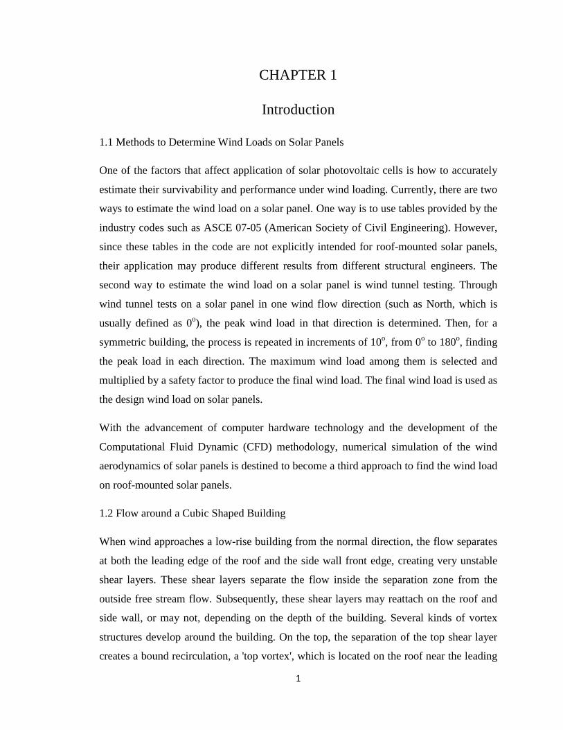
1.1 Methods to Determine Wind Loads on Solar Panels

One of the factors that affect application of solar photovoltaic cells is how to accurately

estimate their survivability and performance under wind loading. Currently, there are two

ways to estimate the wind load on a solar panel. One way is to use tables provided by the

industry codes such as ASCE 07-05 (American Society of Civil Engineering). However,

since these tables in the code are not explicitly intended for roof-mounted solar panels,

their application may produce different results from different structural engineers. The

second way to estimate the wind load on a solar panel is wind tunnel testing. Through

wind tunnel tests on a solar panel in one wind flow direction (such as North, which is

usually defined as 0o), the peak wind load in that direction is determined. Then, for a

symmetric building, the process is repeated in increments of 10o, from 0o to 180o, finding

the peak load in each direction. The maximum wind load among them is selected and

multiplied by a safety factor to produce the final wind load. The final wind load is used as

the design wind load on solar panels.

With the advancement of computer hardware technology and the development of the

Computational Fluid Dynamic (CFD) methodology, numerical simulation of the wind

aerodynamics of solar panels is destined to become a third approach to find the wind load

on roof-mounted solar panels.

1.2 Flow around a Cubic Shaped Building

When wind approaches a low-rise building from the normal direction, the flow separates

at both the leading edge of the roof and the side wall front edge, creating very unstable

shear layers. These shear layers separate the flow inside the separation zone from the

outside free stream flow. Subsequently, these shear layers may reattach on the roof and

side wall, or may not, depending on the depth of the building. Several kinds of vortex

structures develop around the building. On the top, the separation of the top shear layer

creates a bound recirculation, a 'top vortex', which is located on the roof near the leading

2

edge. This top vortex creates a high negative pressure zone on the roof. At the front of the

building, near the base of the windward wall, a horseshoe vortex is generated due to the

roughness of the floor and presence of the obstacle. Along both sides, a side vortex

occurs due to the flow separation at the sidewall leading edge, which originates from the

channel floor. At the back of the cube, an arch-shaped vortex develops, which is confined

by the side flow, top flow and leeward wall. When the wind is at an oblique angle, a

conic vortex develops due to the presence of the two roof edges. These highly unstable

vortices create the highest negative pressure on the roof [18]. Due to the existence of a

pressure gradient and roughness of the upstream terrain, winds are usually gusty and

unsteady. The peak pressure on the surface of a building created by gusty winds has an

important role on wind loading on the building, and the magnitude of the peak pressure

may be much higher than the mean value of the pressure [11].

1.3 Previous Predictions of Pressure Distribution on a Cube Building

Shuzo [31] has simulated natural boundary layer flow over a cube using the k-ε

turbulence model [14] with different boundary conditions and levels of mesh fineness. He

found that the turbulent kinetic energy in the separation region is over-estimated.

Richards [25] has reviewed the problem of flow around a cube in the Computational

Wind Engineering 2000 Conference Competition. Reynolds Averaged Navier-Stokes

(RANS) models, in particular k-ε standard, k-ε RNG [39] and k-ε MMK [34] were

implemented. On the windward and leeward face, both horizontal and vertical centreline

pressure match well with full scale data. However, on the roof, the numerical results

deviate significantly from full scale data. On the side face, the k-ε RNG performs better

than the other two models. The velocity field prediction is noticeably better than the

pressure prediction. Kӧse and Dick [12] used RANS models (k-ε standard, k-ω SST [20])

to predict the pressure coefficient distribution around a 6 m high building and compared

their results with experimental data. At both the windward face and leeward face on the

symmetry plane, the RANS models gave good prediction in pressure. However, at the

roof, the difference between numerical simulation and measurement is large. The

prediction of velocity field is reasonably good, except in the wake region.

3

Using Large Eddy Simulation (LES) of bluff body flow, Shah and Ferziger [29]

simulated fully developed channel flow around a cube, based on the experiments of

Martinuzzi and Tropea [18]. The mean velocity distribution contour at the symmetry

plane has good agreement with the experiment result. The time-averaged streamwise

turbulence also has a good match with experimental data. Unfortunately, no pressure

coefficient distribution was presented. Nozawa and Tamura [23] predicted the mean,

root-mean-square (RMS) and peak pressure coefficient distribution on a low-rise building

under natural boundary layer flow using LES with dynamic version [7] of the

Smagorinsky-Lilly subgrid model [15]. The Reynolds number based on building height

and upstream velocity at building height was 2x104 and the inlet fluctuation was

introduced from a separate LES simulation, based on the technique proposed by Lund et

al. [17]. Compared with experimental data, the mean pressure coefficient showed good

accuracy, the RMS value had a reasonable match except on the roof area near the leading

edge, and the peak value was within the range of full scale measurement.

Kӧse and Dick [12] used a Detached Eddy Simulation (DES) model with RANS model of

k-ω-SST [20] to predict flow over a cube at Reynolds number of 4x104 and 4x106. At the

lower Reynolds number, DES could predict the velocity field very accurately.

Unfortunately, there was no pressure coefficient comparison between DES and

experimental data. At the higher Reynolds number, 4x106, the DES model failed to

predict the pressure coefficient on the roof. Haupt et al. [10] used DES with the Spalart-

Allmarar (SA) option [33] and zonal DES [16] to simulate atmospheric boundary layer

flow over a cube with Reynolds number of 4x106. Both DES and zonal DES have the

capability to predict the pressure coefficient at the windward face and leeward face.

However, the pressure coefficient on the roof is not so good, although zonal DES gives

much better prediction than DES.

1.4 Prediction of Wind Load on a Roof Mounted Solar Panel by Wind Tunnel Test

Adrian [1,2] conducted wind tunnel tests on solar panel arrays installed on the roof of a

five-story building model. He found that a parapet greatly reduced the wind speed on

surface of the solar panels, while the turbulence intensity remains the same. The

difference between the measure of pressure with pneumatic average and calculated mean

4

pressure is negligible. The sheltering effect of the first row of solar panels and the

building itself on the second row of panels is significant. Graeme et al. [9] conducted a

parametrical study of the wind load change on flushed mounted solar panels on a flat roof

with the change of solar panel height and lateral distance. He found the change of vertical

distance from the solar panel to the roof (from 6 mm to 14 mm with scale of 100) and the

lateral distance between each panel (4 mm to 8 mm with the scale of 100) have only a

minor effect on the wind load, except at the roof leading edge.

1.5 Prediction of Wind Load on a Roof Mounted Solar Panel by CFD

Bronkhorst et al. [5] conducted three-dimensional CFD simulations with the k-ε RNG

model and the Reynolds Stress Model (RSM) [13]. The solar panel model was made in a

solid block with scale of 1:50 and tilt angle of 35o. The building is 30 m in breadth, 40 m

in depth and 10 m in height. A structured mesh was used in the simulation and, at the

computational domain inlet, atmospheric boundary layer velocity and turbulent intensity

profiles were implemented. After comparison with wind tunnel test results, the authors

found that the median pressure coefficient predicted by k-ε RNG had 39% difference with

the experiments, while the Reynolds Stress Model had a difference of 35%. In the wake

of the solar panel row, the agreement was even worse due to the incorrect prediction of

the separation zone. Zhou and Zhang [40] conducted a three-dimensional CFD simulation

using finite element software, ADINA, to investigate the difference between wind loads

on a roof with and without solar panels installed. They found that the wind load increased

significantly due to installation of the solar panels.

1.6 Conclusions

RANS models (k-ε RNG and k-ω-SST) and DES with a shear stress transport (SST) or

Spalart-Allmaras (SA) option can predict the pressure distribution at the windward face

and leeward face. However, the prediction on the roof is problematic. LES can accurately

predict the pressure distribution on the roof and it provides reasonable results for the

RMS value only when the Reynolds number is low. RANS models (k-ε RNG and RSM)

do not provide an accurate pressure distribution on roof-mounted solar panels.

5

1.7 Objectives of the Thesis

Based on a search of the literature, it appears that there are no studies on LES and DES

simulations of the wind load on roof-mounted solar panels, and no CFD simulations on

wind load prediction with a fully unstructured mesh. In the current thesis, due to

complexity of the geometry of solar panel arrays, a fully unstructured mesh will be

applied and investigated. Two validation cases and one industrially sponsored project will

be simulated. The two validation cases will be simulated using most of the well-known

RANS models, a DES model and an LES model. For the industrial project the k-ω-SST

model, which shows the best performance, and DES will be used to predict the wind load.

Finally, the wind loading on three solar panel configurations will be predicted by the k-ω-

SST model. These three configurations account for i) an increase in lateral distance (gap)

between solar panels from 0 to 2.5 inches, ii) elevation of the solar panel array by 6

inches off the roof, and iii) elevation of the solar panel array to the same level of a 2.5

foot installed parapet.

The first validation case concerns using RANS models, DES and LES to predict the

pressure coefficient distribution on a cube in an atmospheric boundary layer flow. Results

are compared with wind tunnel tests [31]. The second validation case uses these same

models to predict the mean wind load and peak wind load on a canopy under similar flow

conditions as the cube. The results from these simulations are compared with

experimental data of Ginger and Letchford [8]. The calculated peak force from the LES

and DES simulation results is based on the method of covariance integration [8].

6

CHAPTER 2

Pressure Coefficient on a Cube in an Atmospheric

Boundary Layer

2.1 Flow Problem Description

Shuzo [31] performed both wind tunnel tests and numerical simulations on the flow over

a cube with 200mm length. In numerical simulations of flow over surface-mounted

objects, it is important to ensure that the approaching flow accurately represents the

physical situation. The experimental results of Shuzo [31] and the simulation results from

the current study for the upstream velocity profile and turbulent intensity profile are

shown in Figures 2-1a and 2-1b, respectively. These figures show the velocity and

turbulent kinetic energy at the cube location, but without presence of the cube. In these

figures, h is cube height and uref is the velocity at cube height at the location of the cube.

The non-uniform unstructured mesh used in these calculations is able to accurately

capture the velocity all the way to the bed. However, there is noticeable disagreement

between the numerical simulation and wind tunnel data near the bed for the turbulent

kinetic energy. This is likely due to inaccuracies in both the experimental and numerical

methodologies, because of difficulties with near-bed measurements of turbulence and the

coarse mesh near the bed used in the simulation.

0.0

0.5

1.0

1.5

2.0

0.40 0.90 1.40

Expt. [31]

k-ω-SST (a)

z/h

u/uref

7

Fig. 2-1 Comparison of experimental results and numerical prediction (k-ω-SST) at cube

location, without presence of the cube, (a) velocity profile; (b) turbulent kinetic energy

2.2 Governing Equations

The equations that govern the unsteady flow of an incompressible fluid are [35]

𝜕𝑢𝑖𝜕𝑥𝑖

= 0 (2-1)

𝜌 𝜕𝑢𝑖𝜕𝑡

+ 𝜌 𝜕(𝑢𝑗𝑢𝑖)𝜕𝑥𝑗

= − 𝜕𝑝𝜕𝑥𝑖

+ 𝜕𝜕𝑥𝑖

(𝜇 𝜕𝑢𝑖𝜕𝑥𝑗

) (2-2)

where ui, p, ρ and µ denote the velocity components in the Cartesian coordinate system

xi , (i = 1, 2, 3), pressure, density and dynamic viscosity, respectively. Equations (2-1)

and (2-2) are the well-known Navier-Stokes (N-S) equations.

There are three ways to treat these equations for turbulent flows. One method, which

forms the basis for Reynolds Averaged Navier-Stokes Equations (RANS), is to perform

time-averaging. The second method uses a spatial filtering operation, which is the

methodology used for Large Eddy Simulation (LES). The third method is Direct

0.0

0.5

1.0

1.5

2.0

2.5

0.00 0.01 0.02 0.03 0.04

Expt. [31]

k-ω-SST (b)

8

Numerical Simulation (DNS). DNS is extremely computationally expensive and is not

considered in this thesis.

2.2.1 Reynolds Averaged Navier-Stokes (RANS)

If the N-S equations are time-averaged, second-order moment terms, which represent the

fluctuation of Reynolds stress, will arise in the equations. This procedure adds six new

unknowns, the Reynolds stresses, to the set of four equations above. Turbulence models

have been developed to close the time-averaged N-S equations. There are models based

on one equation, e.g., Spalart-Allmaras [32] (see eqn. (A-2) in Appendix A), and two

equations, e.g., k-ε standard developed by Launder and Spalding [14] (see eqns. (A-3),

(A-4)); RNG, renormalization group devise by Yakhot et al. [39] (see eqns. (A-5), (A-6));

Realizable, proposed by Shih et al. [30] (see eqns. (A-3), (A-7)); k-ω, proposed by

Wilcox [37] (see eqns. (A-8), (A-9)); k-ω-SST, devised by Menter [20] (see eqns. (A-10),

(A-11)). The Reynolds stresses are calculated based on the assumption that there exists an

analogy between the action of viscous stresses and Reynolds stresses on the mean flow,

which is referred to as the Boussinesq assumption (see eqn. (A-1)).

Both one equation and two equation models are referred to as turbulent viscosity models

and are based on the assumption that the turbulent viscosity is isotropic in space. This

assumption is not valid in many flow situations. To overcome this deficiency the

Reynolds Stress Model (RSM) (also called Differential Stress Model) proposed by

Launder et al. [13], has been developed (see eqn. (A-12)). This model uses a stress

transport equation for each component of the Reynolds stress tensor to solve the

anisotropic problem of the flow.

2.2.2 Large Eddy Simulation (LES)

The second method to close the N-S equations is to conduct a spatial filtering operation

on the N-S equation. Eddies larger than the filter space will be calculated while the

smaller eddies will be simulated by a subgrid-scale model. The characteristics of large

eddies are more problem dependent, which are primarily determined by the geometry of

the flow, while small eddies are more isotropic, and are suitable for modeling. This is the

essence of large eddy simulation (LES). LES falls between DNS and RANS in terms of

9

the fraction of the resolved scales. Though in theory it is possible to resolve the whole

spectrum of the turbulence scales using DNS, in the current stage of development, it is

impossible to conduct DNS for practical industrial use.

The Smagorinsky subgrid-scale (SGS) model, based on assumption of the Boussinesq

hypothesis, has been used in current research. The subgrid stresses are calculated by

equation (A-13).

The dynamic SGS model proposed by Germano et al. [7] is used to determine the SGS

stresses with two different filtering operations, with cutoff widths ∆1 and ∆2 (see eqn. (A-

14)). Since, in the case of bluff body flow problems this option usually gives better

simulation results [22], it is used in the current work.

Large Eddy Simulation (LES) need much more computing power than RANS models,

but it gives more accurate results than the RANS model in the case of bluff body flow

[22].

2.2.3 Detached Eddy Simulation (DES)

In the Detached Eddy Simulation (DES) approach, the unsteady RANS models are

employed in the boundary layer and the LES models is applied in the separated regions.

DES models have been specially designed to address high Reynolds number wall-

bounded flows, where the cost of computation is very high when using LES over the

entire flow field. The computational cost for DES is lower than LES but is higher than

RANS.

Fluent offers three types of RANS model for DES, the Spalart-Allmaras model, the k-ε

Realizable model and the k-ω-SST model. In the current research, k-ω-SST based DES

proposed by Menter et al. [20] will be used. The reason for choosing this model is that the

k-ω-SST model demonstrates relatively better prediction in the two validation cases.

10

2.3 Near-Wall Treatment

Traditionally, there are two approaches to model the near-wall flow region. One approach

is to use the “standard wall function”, which uses an empirical equation to “bridge” the

viscous layer to the outer layer, and the viscous region is not resolved [3]. Another

approach is to use a wall model near the wall [3], so the flow inside the three layers all

get resolved. The mesh near the viscous layer usually is very fine. Details of these models

can be found in Appendix B.

2.4 Computational Domain and Test Cases

Setting the size of the computational domain is not an easy or straightforward task.

Choosing the computational domain too large will waste computational resources and

time, while picking too small of a computational domain will give inaccurate solutions.

Three domain sizes are listed in Table 2-1. Domain II is recommended in the Best CFD

Performance Guide [6], domain I was reported by Köse and Dick [12] to give similar

simulation results as those from a much larger domain size, and domain III is considered

here to see whether this large domain will improve the simulation results. These three

domain sizes are used for the initial simulation with one of the RANS model, k-ω-SST,

which is selected due to the accuracy in the Cp prediction, to be demonstrated below.

Figures 2-2 and 2-3 show domain II layout in the horizontal plane and cross-section,

together with the boundary conditions imposed on the flow. From these initial tests with

the k-ω-SST model, after comparison with experimental data, it was determined that

domain II is the most suitable and therefore will be used for further simulations. The

simulation results of Cp on the symmetry plane of the cube are shown in Fig. 2-4.

Table 2.1 Extent of computational domain (h: cube height)

Domain # of cells

Upstream length

Downstream length

Lateral Vertical

I 220,000 3h 10h 3h 3h II 400,000 5h 20h 5h 5h III 850,000 5h 30h 10h 10h

11

Fig. 2-2 Computational domain II (horizontal layout, not to scale)

Fig. 2-3 Computational domain II (cross-sectional layout, not to scale)

5h h 5h

5h

h

Wall (no slip)

12

Fig.2-4 Effect of computational domain size on Cp distribution

2.5 Boundary Conditions

The velocity at the inlet is taken as

𝑢𝑧 = 𝑢𝑟𝑒𝑓( 𝑧𝑧𝑟𝑒𝑓

)𝛼 (2-3)

where 𝑢𝑧 , 𝑢𝑟𝑒𝑓 , 𝑧𝑟𝑒𝑓, 𝑧, 𝛼 are streamwise velocity component, reference velocity,

reference height, elevation and exponent, respectively. The turbulent kinetic energy and

dissipation rate are determined from

𝑘 = 32

(𝑢𝑟𝑒𝑓𝑇𝑖)2 (2-4)

𝜀 = 𝐶𝜇3/4 𝑘3/2

𝑙 (2-5)

where Cμ is a constant and Ti is the turbulence intensity, as recommended in the literature

[35]. The definition of specific dissipation rate and viscosity ratio are given by

𝜔 = 𝜀𝑘𝐶𝜇

(2-6)

-1.0

-0.5

0.0

0.5

1.0

0.0 1.0 2.0 3.0

Expt. [31]

k-ɷ-SST_domain_I

k-ɷ-SST_domain_II

k-ɷ-SST_domain_III

x/h

A

B

C

A B C

13

𝜇𝑡𝜇

= 𝜌𝜇𝐶𝜇

𝑘2

𝜀 (2-7)

For DES and LES, the inlet turbulence is generated using the vortex method [19]. The

downstream exit is specified as an outflow. The top surface, side surfaces, bottom surface

and cube surface are all considered as no-slip walls.

For k-ε standard, k-ε RNG, k-ε Realizable and Reynolds Stress Model, scalable wall

function [3] is used to avoid deterioration of the standard wall function when the mesh

cells gets too fine.

For LES, the Werner-Wengle wall function [36] is used to alleviate the strict fine mesh

requirement near the wall for high Reynolds number wall-bounded flows.

2.6 Mesh Topology

A tetrahedral mesh has been constructed to discretize the computational domain, using

Gambit 2.4. A tetrahedral mesh is not commonly used in the wind engineering literature

due to its lower efficiency of discretization of space compared with a structured mesh.

But it has the important advantage of flexibility. In this work a non-uniform unstructured

mesh has been used with a finer mesh implemented in regions of high gradients. The

mesh layout in the vertical symmetry plane for the present simulations is illustrated in Fig.

2-5. There are approximately 25 cells along each edge, with the total number of cells

reaching about 400,000.

Fig. 2-5 Tetrahedral mesh around the cube

14

2.7 Numerical Setup

For most of the RANS models (except RSM), third-order accuracy is used for spatial

discretization of the convection terms in both the momentum equations and turbulence

equations, while second-order accuracy is used for the pressure interpolation. The

solution algorithm uses pressure based, pressure-velocity coupling. For RSM, the second-

order upwind scheme is used for convection terms, while the solution algorithm uses

pressure based, segregated, SIMPLE [24]. For the LES and DES simulations, bounded

central differencing is used for momentum equations. The time discretization is implicit

second-order. The Courant-Friedrichs-Lewy number is around 5 for LES and around 10

for DES. The drag coefficient and a continuity equation residual less than 10-7 have been

used as the converge criteria.

2.8 Simulation Results

2.8.1 Cp Distribution in Vertical Symmetry Plane of the Cube

The pressure coefficient, Cp, is defined as

𝐶𝑝 = (𝑝−𝑝0)12𝜌𝑢𝑟𝑒𝑓

2 (2-8)

where p and p0 are static pressure and reference pressure, respectively. The simulation

results from each of the turbulence models are compared with experimental data of [31]

in Figs. 2-6, and 2-7.

a). Windward symmetry plane

The k-ω-SST model shows the best performance for the prediction of Cp on the front of

the cube, closely matching with experimental data as seen in Fig. 2-6a. The Reynolds

Stress Model ranks second, as illustrated in Fig. 2-6b. Although it could not predict the

Cp increase near the ground level, which is due to the effect of front wall recirculation,

for most of the front face, RSM yields a good overall prediction. The least accurate

prediction is the k-ω standard result which, as shown in Fig. 2-6a, over-predicts Cp by

four-fold. The second worst performance is k-ε standard (Fig. 2-7a), over-predicting Cp

by a factor of two. In fact, these models predict a Cp value much great than 1. The reason

15

for this will be discussed in section 2.8.2. The Spalart-Allmaras model (Fig. 2-6b), k-ε

RNG and k-ε Realizable (Fig. 2-7a) have similar performance., all of them predict the

correct shape of the Cp curve only slightly over-predict the Cp near the leading edge

region. Both DES-SST and LES (Fig. 2-7b) accurately predict Cp on the windward face,

although LES appears slightly closer to the experimental data.

b). Roof symmetry plane

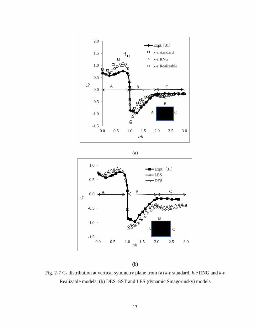
Considering only the roof portion of the cube, RSM has the best prediction of Cp, closely

matching the experimental data (Fig. 2-6b); k-ω-SST and k-ε RNG also both give good

prediction on the roof. The k-ɷ-SST model slightly under-predicts the suction pressure

near the leading edge, while k-ε RNG slightly over-predicts the suction pressure. The SA

model over-predicts the suction pressure near the leading edge and under-predicts it over

the main region. The k-ω standard, k-ε standard and k-ε Realizable fail to predict the Cp

on the roof; they significantly over-predict the suction pressure on the leading edge and

under-predict the suction pressure in the remaining region. Both DES-SST and LES

slightly over-predict the suction pressure on the roof, but still are in an acceptable range.

DES-SST results appear to be closer to the experimental data than LES.

c). Leeward symmetry plane

On the leeward side, the experimental Cp shows constant negative value (around -0.2)

from the top of the cube to ground level in the symmetry plane, while all the RANS

models show only a slight deviation from this constant value. In general, all the RANS

models not only have similar performance but also are very close to the experimental data.

Both DES and LES significantly over-predict the suction pressure along the leeward wall.

16

(a)

(b)

Fig. 2-6 Cp distribution at vertical symmetry plane from (a) k-ω standard and k-ω-SST

models; (b) Reynolds Stress Model (RSM) and Spalart-Allmaras (SA) model

-1.5

-1.0

-0.5

0.0

0.5

1.0

1.5

2.0

2.5

3.0

0.0 0.5 1.0 1.5 2.0 2.5 3.0

Expt. [31]

k-ɷ-SST

k-ɷ standard

-1.5

-1.0

-0.5

0.0

0.5

1.0

1.5

0.0 0.5 1.0 1.5 2.0 2.5 3.0

Expt. [31]RSMSA

17

(a)

(b)

Fig. 2-7 Cp distribution at vertical symmetry plane from (a) k-ε standard, k-ε RNG and k-ε

Realizable models; (b) DES–SST and LES (dynamic Smagorinsky) models

-1.5

-1.0

-0.5

0.0

0.5

1.0

1.5

2.0

0.0 0.5 1.0 1.5 2.0 2.5 3.0

Expt. [31]

k-ε standard

k-ε RNG

k-ε Realizable

Cp

-1.5

-1.0

-0.5

0.0

0.5

1.0

0.0 0.5 1.0 1.5 2.0 2.5 3.0

Expt. [31]LESDES

A

B

C

A B C

18

2.8.2 Flow Pattern around the Cube

The streamtraces pattern near the cube in the vertical symmetry plane and a horizontal

plane near the ground, predicted by the seven RANS models, DES-SST and LES, are

presented in Figs. 2-8 to 2-16. Most models have predicted the ring vortex, roof

separation bubble, side separation and wake recirculation, but the shapes and locations

are different from each other. As seen in Fig. 2-9a and Fig. 2-12a, both k-ε standard and

k-ω standard fail to predict the roof separation. This is the reason that the predicted Cp

from these models rises to a value greater than 1. The flow patterns from RANS models

are more symmetrical than those from DES-SST and LES. The reason for this may be

that the simulation times for the DES-SST and LES are not long enough. Since there is

no experimental information about the streamtraces pattern, one should be cautious to

speculate which model predicts the more realistic flow pattern. Nevertheless, based on

the Cp discussions above, it appears that the k-ω-SST provides the most reliable results

over the entire cube.

(a)

(b)

Fig. 2-8 Streamtraces predicted by Spalart-Allmaras model, (a) vertical symmetry plane;

(b) horizontal plane at 0.125h

19

(a)

(b)

Fig. 2-9 Streamtraces predicted by k-ε standard model, (a) vertical symmetry plane;


(a)

(b)

Fig. 2-10 Streamtraces predicted by k-ε RNG model, (a) vertical symmetry plane;


20

(a)

(b)

Fig. 2-11 Streamtraces predicted by k-ε Realizable model, (a) vertical symmetry plane;


(a)

(b)

Fig. 2-12 Streamtraces predicted by k-ω standard model, (a) vertical symmetry plane;


21

(a)

(b)

Fig. 2-13 Streamtraces predicted by k-ω-SST model, (a) vertical symmetry plane;


(a)

(b) Fig. 2-14 Streamtraces predicted by Reynolds Stress Model, (a) vertical symmetry plane;


22

(a)

(b)

Fig. 2-15 Streamtraces predicted by DES-SST model, (a) vertical symmetry plane;


(a)

(b)

Fig. 2-16 Streamtraces predicted by LES (dynamic Smagorinsky), (a) vertical symmetry

plane; (b) horizontal plane at 0.125h

23

2.8.3 Flow Recirculation Length

Unfortunately, there is no reported experimental data about the recirculation length for

the reattachment behind the cube. The flow recirculation length predicted by different

models has been summarized in Table 2.2. From this table, one can see that the

recirculation length predicted from the RANS models is larger than that from DES or

LES. This observation is consistent with information reported in the literature [27], where

the result from LES is closer to experimental data in the case of a square cylinder.

Table 2.2 Flow recirculation length in the wake region (h: cube height)

Model Recirculation length

Spalart-Allmaras 1.80h

k-ω standard 1.75h

k-ω-SST 2.25h

k-ε standard 1.63h

k-ε RNG 1.95h

k-ε Realizable 1.85h

Reynolds Stress 1.80h

DES-SST 1.35h

LES (Dynamic Smagorinsky) 1.50h

2.9 Discussion and Conclusions

As mentioned above, there is less information reported in the literature about numerical

simulations over cubes with unstructured meshes, for both RANS models and LES. The

main reasons may be the ineffective discretization of space with an unstructured mesh

and the general lack of familiarity of unstructured meshes in this type of application.

Nevertheless, through construction of the computational model and setting up of the mesh,

we have found that the unstructured mesh is much more flexible than a structured mesh.

However, successful implementation of an unstructured mesh requires good experience

using some important mesh parameters, such as cell growth rate, maximum cell size and

size function type, etc.

24

The simulation results from both DES-SST and LES are not as good as those from k-ω-

SST and RSM. This may be due to the fact that the mesh near the cube is still too coarse

for the LES case. Usually the y+ value required for LES is around 1 [22], which

consequently requires huge computing power for the high Reynolds number in the

current simulations. Although the Werner-Wengle wall function has been implemented, it

may be that the mesh is still too coarse to capture the near-wall region with the current

mesh methodology. For the DES case, the communication between the RANS model and

the LES model at the interface might be an issue affecting the prediction accuracy.

Computational domain size of type A is too small, and the boundary conditions will

greatly affect the simulation results on both the roof and leeward side of the cube. Type B,

which is recommended by the Best CFD Performance Guide [6], is acceptable for the

simulation results when compared with a larger domain size such as type C, since type C

domain will only slightly improve the results on the roof region, and does not change the

results on either the windward or leeward sides.

Amongst the RANS model mentioned in this chapter, both k-ω-SST and the Reynolds

Stress Model are the most suitable models to predict wind load on a building. They

accurately predict the pressure coefficient on the windward wall, the roof and on the

leeward wall. The Reynolds Stress Model needs much more computing power than the k-

ω-SST model. The k-ε standard, k-ε Realizable and k-ω standard are not suitable for bluff

body flow simulations. Spalart-Allmaras model and k-ε RNG give similar prediction

performance, and compare reasonably well with experimental data.

In this thesis, the velocity field obtained from the numerical simulations has not been

compared with experimental data. The velocity field predictions are usually more

accurate than the pressure field. However, for the current purpose, the pressure

distribution is more important than the velocity field in regards to the final objectives of

this thesis. It is also important to keep in mind that both the wind tunnel tests and the

numerical simulation are performed on scale models.

25

CHAPTER 3

Wind Load on a Free Standing Roof in an

Atmospheric Boundary Layer

The effects of turbulence modeling on the numerical simulation of wind load on a free

standing roof are investigated in this chapter. The main objective is to predict the wind

load on the mid-section of a free standing inclined roof, also referred to as a canopy,

under atmospheric boundary layer flow. Nine turbulence models are considered, seven

Reynolds-Averaged Navier-Stokes (RANS) equation models, Large-eddy Simulation

(LES) with dynamic Smagorinsky subgrid model and Detached Eddy Simulation (DES-

SST). The RANS models are Spalart-Allmaras (SA), k-ε standard, RNG and Realizable,

k-ω standard, k-ω-SST and Reynolds Stress Model (RSM). The difference in mean

pressure coefficient (Cp) across the roof, at different wind directions, obtained from each

RANS model with two levels of mesh fineness, has been compared with experimental

data.


For the current study, wind tunnel test data corresponding to an atmospheric boundary

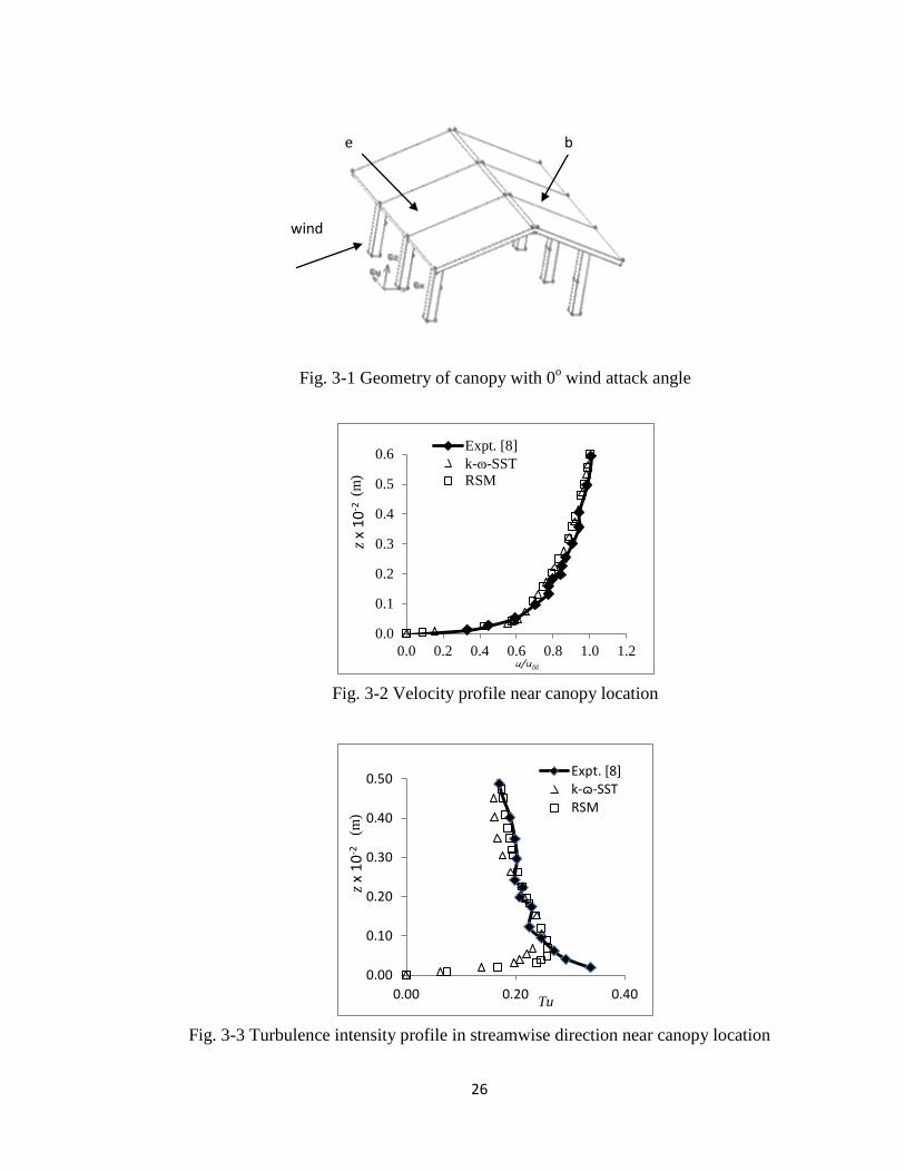
layer for a suburban terrain has been extracted from literature [8]. A schematic of the

flow problem is shown in Fig. 3-1. The full-scale dimension of the canopy is 30 m x 30 m,

with roof slope of 22.5o and support height of 10 m. The model scale in the numerical

model is the same as in the wind tunnel test, 1:100. Velocity and streamwise turbulence

intensity profiles at the location of the canopy, but without the presence of the canopy,

are shown in Fig. 3-2 and Fig. 3-3, respectively. For consistency with the experiments,

the velocity in Fig. 3-2 is normalized by the velocity at 60 m in real scale, u60.

Numerically simulated results from k-ω-SST and RSM have been included for

comparison.

26

Fig. 3-1 Geometry of canopy with 0o wind attack angle

Fig. 3-2 Velocity profile near canopy location

Fig. 3-3 Turbulence intensity profile in streamwise direction near canopy location

0.0

0.1

0.2

0.3

0.4

0.5

0.6

0.0 0.2 0.4 0.6 0.8 1.0 1.2

Expt. [8]k-ɷ-SST RSM

(m)

z x 1

0-2

0.00

0.10

0.20

0.30

0.40

0.50

0.00 0.20 0.40

Expt. [8]k-ɷ-SST RSM

Tu

z x 1

0-2

(m)

e

wind

b

27


The equations that govern the unsteady flow of an incompressible fluid are [35]


= 0 (3-1)



= − 𝜕𝑝𝜕𝑥𝑖

+ 𝜕𝜕𝑥𝑗


) (3-2)


xi , (i = 1, 2, 3), pressure, density and dynamic viscosity, respectively.

These equations are the same as those used in Chapter 2. A discussion of the turbulence

models used with these equations can be found in section 2.2 and a detailed description of

these models is given in Appendix A. Discussion of the wall treatment and

implementation of different models is provided in Appendix B.

3.3 Computational Domain

The horizontal and cross-section layouts of the computational domain are illustrated in

Fig. 3-4 and Fig. 3-5, respectively, where h is the height of the canopy support.

Fig. 3-4 Computational domain (horizontal layout, not to scale)

28


The boundary conditions associated with the flow over the canopy are identical to those

for flow over the cube building. These conditions are discussed in section 2.5 and

mathematically formulated as equations (2-3) to (2-7).

3.5 Mesh Topology

A tetrahedral mesh, with two levels of refinement, is used for the RANS models. For the

coarse mesh, the smallest cell size is around 15 mm in the region near the canopy, while

in the far region the cell size is around 70 mm, with total cell number of approximately

150,000. For the finer mesh, the smallest cell size is around 7 mm in the region close to

the canopy, with 70 mm cell size farther away, with a total of approximately 300,000

cells. The DES and LES models will only be implemented on the coarse mesh due to the

computational power limitation. The fine mesh (7 mm) in the vicinity of the canopy is

shown in Fig. 3-5.

Fig.3-5 Tetrahedral mesh around the canopy in the cross-section layout

3.6 Numerical Setup

The numerical setup for this problem is the same as that for the cube building in Chapter

2. Except for RSM, the convective terms in the RANS models are discretized with third-

order accuracy. Second-order accuracy is used for the pressure interpolation and the

29

solution algorithm uses pressure based, pressure-velocity coupling. For RSM, the second-

order upwind scheme is used for convection terms, while the solution algorithm uses

pressure based, segregated and SIMPLE [24]. Bounded central differencing is used for

momentum equations in the LES and DES simulations. The time discretization is implicit

second-order. The drag coefficient and a continuity equation residual less than 10-7 have

been used as the converge criteria.


3.7.1 Wind Load on the Canopy Roof

Throughout this chapter, the pressure coefficient refers to the area-averaged pressure

coefficient. The pressure coefficient difference on the middle section of the windward

roof, i.e., on plate e in Fig. 3-1, with wind attack angles from 0o to 180o, has been

predicted using the seven RANS models, as well as the DES-SST model and the LES

dynamic Smagorinsky model. The pressure coefficient difference, ∆Cp, is defined as the

difference between the pressure coefficient on the top surface and on the bottom surface

of the roof, that is

∆𝐶𝑝 = (𝑝𝑇−𝑝𝐵)12𝜌𝑢𝑟𝑒𝑓

2 (3-3)

where pT and pB are the area-averaged pressures on the top and bottom of the roof,

respectively. Positive ∆Cp means that the roof plate experiences a downward force, while

a negative ∆Cp indicates an upward force.

a). Simulation results from k-ω, k-ω-SST and Spalart-Allmaras (SA) model

The variations of ∆Cp on plate e, extracted from the coarse mesh simulations (15 mm cell

size around the canopy) using the k-ω standard, k-ω-SST and Spalart-Allmaras models,

are plotted in Fig. 3-6, demonstrating that the k-ω-SST and Spalart-Allmaras models have

much better accuracy than the k-ω standard model in the windward attack direction (from

0o to 90o). The k-ω-SST and SA simulation results at these wind attack angles display

good agreement with the experimental data of Ginger and Letchford [8], except for wind

in the 0o angle of attack direction. At leeward attack angles (from 90o to 180o), k-ω-SST

30

and SA show around 25% deviation from experimental data. The k-ω standard model

results are even less reliable, as seen in Fig. 3-6.

Fig. 3-6 ∆Cp at different wind attack angles predicted by RANS models (coarse mesh near the canopy)

With a finer mesh (7 mm cells around the canopy), k-ω-SST and SA models show no

improvement at windward attack angles. Figure 3-7 illustrates that, although the k-ω

standard model shows noticeable improvement, particularly at 0o, it still deviates much

more from experimental data compared to the other two models. On the leeward side, all

three models show obvious improvement only at 180o attack angle. Among these three

models, the k-ω-SST shows slightly better prediction than the SA model, and much better

than the k-ω standard model. It yields good prediction at wind attack angles from 30o up

to 90o, then starts to deviate from the experimental data from 90o and reaches maximum

deviation at 150o wind attack angle, after which the difference decreases. At 180o, the k-

ω-SST model gives good prediction of ∆Cp. In both levels of mesh refinement, all the

models show the correct ∆Cp prediction at 90o wind attack angle. As seen in Fig. 3-7,

-1.5

-1.0

-0.5

0.0

0.5

1.0

0 30 60 90 120 150 180

Expt. [8]

k-ɷ-SST

k-ɷ

SAΔC

p

αo

31

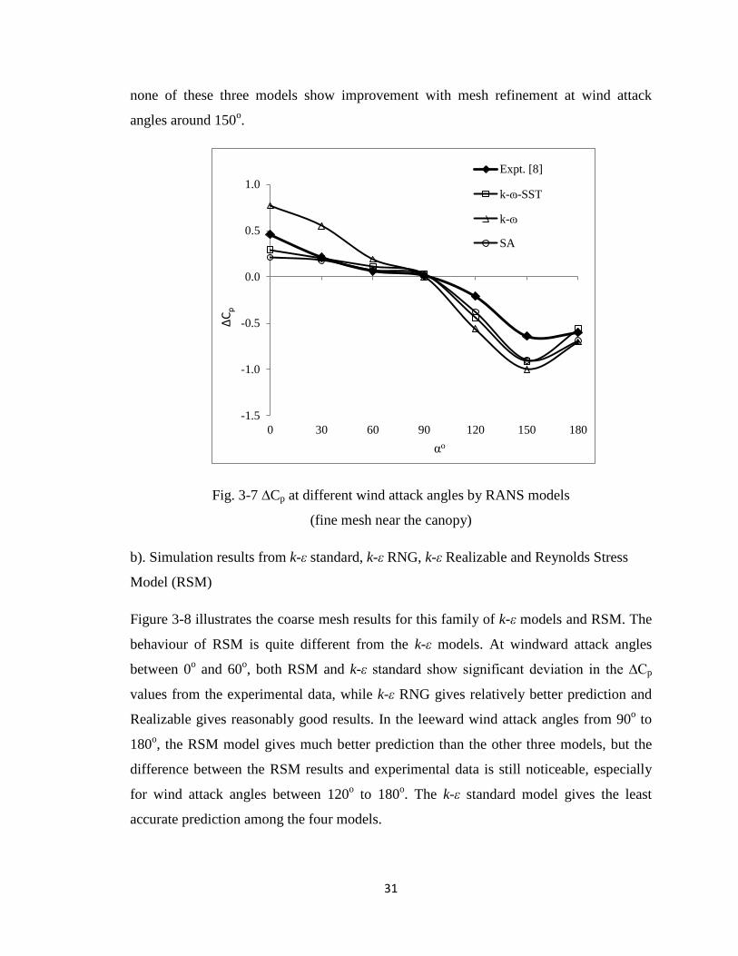
none of these three models show improvement with mesh refinement at wind attack

angles around 150o.

Fig. 3-7 ∆Cp at different wind attack angles by RANS models

(fine mesh near the canopy)

b). Simulation results from k-ε standard, k-ε RNG, k-ε Realizable and Reynolds Stress

Model (RSM)

Figure 3-8 illustrates the coarse mesh results for this family of k-ε models and RSM. The

behaviour of RSM is quite different from the k-ε models. At windward attack angles

between 0o and 60o, both RSM and k-ε standard show significant deviation in the ∆Cp

values from the experimental data, while k-ε RNG gives relatively better prediction and

Realizable gives reasonably good results. In the leeward wind attack angles from 90o to

180o, the RSM model gives much better prediction than the other three models, but the

difference between the RSM results and experimental data is still noticeable, especially

for wind attack angles between 120o to 180o. The k-ε standard model gives the least

accurate prediction among the four models.

-1.5

-1.0

-0.5

0.0

0.5

1.0

0 30 60 90 120 150 180

Expt. [8]

k-ɷ-SST

k-ɷ

SAΔC

p

αo

32


(coarse mesh near the canopy)

Using the finer mesh, there is no improvement in the simulation results of RSM for wind

direction from 0o to 60o. As seen in Fig. 3-9, k-ε RNG and k-ε Realizable improve at 30o

and 60o, but still deviate at 0o. None of these models can accurately capture the ∆Cp

variation with the change of wind attack angle. The simulation result of k-ε standard has

improved with the refined mesh. In leeward wind attack angles, the RSM results show

improvement only at 180o. The simulation results from k-ε RNG and k-ε Realizable do

not improve at any leeward wind attack angle. Figure 3-9 shows that the k-ε standard

simulation has improved slightly at wind attack angle of 180o.

-1.5

-1.0

-0.5

0.0

0.5

1.0

0 30 60 90 120 150 180

Expt. [8]

RSM

k-ε standard

RNG

Realizable

ΔCp

αo

33


(fine mesh near the canopy)

c). Simulation results from DES-SST and LES

Simulations with DES and LES were conducted only with the coarse mesh (cell size of

15 mm) due to limited computational power. From Fig. 3-10, it seems that neither DES

nor LES yields better results than the RANS models. In wind attack angles from 30o to

180o, LES does give a better prediction, especially at wind attack angle of 180o. But, at

wind attack angle of 0o, LES shows much more deviation from the experimental results

than DES-SST.

-1.5

-1.0

-0.5

0.0

0.5

1.0

0 30 60 90 120 150 180

Expt. [8]

RSM

k-ε

RNG

Realizable

ΔCp

αo

34

Fig. 3-10 ∆Cp at different wind attack angles by DES-SST and LES (coarse mesh near the canopy)

The ∆Cp difference on plates e and b can be used to determine the drag coefficient and lift

coefficient. Using the standard deviation of ∆Cp fluctuations, the peak drag and peak lift

can also be calculated by the covariance integration method [8].

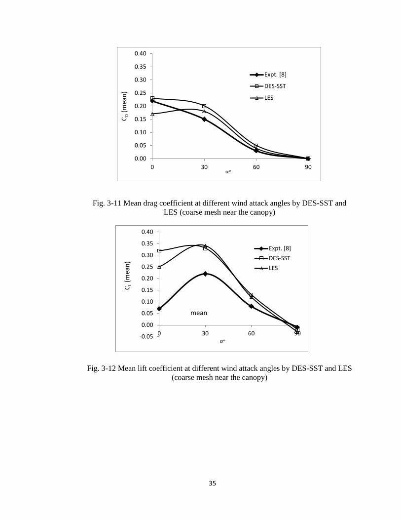
The area-averaged mean loads on plates e and b are illustrated in Fig. 3-11 and Fig. 3-12.

The drag coefficient is better predicted than the lift coefficient by both DES-SST and

LES, and LES performs better than DES-SST. For lift coefficient, the larger deviations

from the wind tunnel test results occur at wind attack angles between 0o and 45o.

For peak loads on plates e and b, shown in Fig. 3-13 and Fig. 3-14, the drag coefficient is

again more accurately predicted than lift coefficient, especially at wind attack angles

from 30o to 90o. The deviation from experimental data for both the peak drag and lift

coefficients at wind attack of 0o is seen in these figures.

-1.0

-0.5

0.0

0.5

1.0

0 30 60 90 120 150 180

Expt. [8]

DES-SST

LES

ΔCp

αo

35

Fig. 3-11 Mean drag coefficient at different wind attack angles by DES-SST and LES (coarse mesh near the canopy)

Fig. 3-12 Mean lift coefficient at different wind attack angles by DES-SST and LES (coarse mesh near the canopy)

0.00

0.05

0.10

0.15

0.20

0.25

0.30

0.35

0.40

0 30 60 90

Expt. [8]

DES-SST

LES

C D (m

ean)

-0.05

0.00

0.05

0.10

0.15

0.20

0.25

0.30

0.35

0.40

0 30 60 90

Expt. [8]DES-SSTLES

mean

C L (m

ean)

36

Fig. 3-13 Peak drag coefficient at different wind attack angles by DES-SST and LES (coarse mesh near the canopy)

Fig. 3-14 Peak lift coefficient at different wind attack angles by DES-SST and LES

(coarse mesh near the canopy)

3.7.2 Velocity Field around the Canopy

Figure 3-15 shows the velocity vector field in the central vertical plane of the canopy

from the k-ω-SST simulation at wind direction of 0o. The flow splits when it reaches the

0.0

0.1

0.2

0.3

0.4

0.5

0.6

0 30 60 90

Expt. [8]

DES-SST

LES

C D (p

eak)

0.0

0.1

0.2

0.3

0.4

0.5

0.6

0.7

0.8

0.9

0 30 60 90

Expt. [8]

DES-SST

LES

CL

(pea

k)

37

front end of the roof, some of the flow moving along the roof top surface without

separation at the top leading edge, while some of the flow separates at the bottom leading

edge due to the slope of the roof. On the roof top, the flow accelerates as it approaches

the roof ridge, and there is no separation occurring in the ridge region. As the air flows

along the top surface of the leeward roof, the flow speed decreases, and the flow

separates as it approaches the middle of the leeward roof.

Because of the shape of the canopy, there is a large counter-clockwise rotating circulation

bubble that forms under the canopy. A downward force and an upward force develop on

the windward roof and the leeward roof, respectively. The downward force comes from

two sources; one is from the direct contact flow along the top surface, which produces

positive pressure due to the slope of roof. The second contribution to the downward force

is due to the separated flow at the leading edge of the bottom surface. The upward force

also comes from two sources; one is the flow separation on the top surface near the lower

part of the leeward roof, the second is the reattachment flow near the lower part of the

bottom leeward roof.

Fig. 3-15 Flow velocity vectors near the canopy at wind attack angle of 0o,

predicted by k-ω-SST

38


As discussed in section 3.7, there are considerable discrepancies between the

experimental data and the computational results for all the turbulence models

implemented in this work. There is no uncertainty report by which to assess the validity

of the wind tunnel test results. Are the test results really representative of the true wind

load on this roof? In the experiments there were only a total of twelve pressure taps for

one section of roof, 10 m x 15 m in size, with six pressure taps evenly distributed on the

top surface and six pressure taps on the bottom surface. From the plots of pressure

coefficient contours on the plates e and b shown in Fig. 3-16 and Fig. 3-17, one can easily

observe that the pressure is not evenly distributed on the roof. Since, in the experiments,

there are no pressure taps near the edge and ridge regions of the roof, the area-averaged

loads calculated from the measurements may not be representative of the real wind loads.

This is the main reason for the difference between the numerical simulation and the wind

tunnel results.

Fig. 3-16 Pressure coefficient contours for top of plate e (left) and plate b (right)

39

Fig. 3-17 Pressure coefficient contours for bottom of plate e (left) and plate b (right)

The numerical simulations with different turbulence models produce results that vary

between each model and between the models and the wind tunnel test results. However,

these models show some common features. They all accurately predict the Cp difference

at wind attack angle of 90o (when wind attack angle is parallel to the roof ridge line).

They all show significant deviation from the wind tunnel results at wind attack angle of

150o. The smallest deviation is about 25%, which comes from the RSM and k-ω-SST

models. In windward attack angles (from 0o to 90o), k-ω-SST, k-ε RNG and SA models

show better prediction, while in leeward attack angles (from 90o to 180o), RSM shows

relatively better results. No model demonstrates good prediction at all wind attack angles.

The k-ω-SST model gives slightly better prediction results compared with the other

models. Neither DES-SST nor LES improved the simulation results in terms of mean

wind load. In the leeward direction, LES gives a slightly better prediction than the DES-

SST model. For both DES-SST and LES models, the drag prediction is better than the lift

prediction. For peak wind load, LES performs slightly better than DES-SST for both drag

and lift coefficient.

40

CHAPTER 4

Mean and Peak Wind Load on Flat Roof Mounted Solar Panels in

an Atmospheric Boundary Layer (Basic Case)

The two validation cases discussed in Chapters 2 and 3 have shown that both k-ω-SST

and RSM give better prediction of mean wind loading than other RANS models in bluff

body flow, and either DES-SST or LES can be used to simulate both the mean and peak

wind load. In this chapter, considering the building dimensions and the geometrical

complexity of solar panel arrays, only the k-ω-SST model will be used to predict the

mean wind load on solar panels, employing three levels of mesh fineness. DES-SST will

be used to predict both mean and peak wind load on the coarsest mesh due to

computational power limitations. Wind load will be predicted from these two models

with wind attack angles from 360o to 180o with increment angle of 30o. Additionally,

wind attack angles of 340o and 320o will be tested to disclose the wind load change at the

most critical wind attack angle of 330o (based on our simulations and wind tunnel test

results). Wind attack angle of 360o is defined as wind approaching the rear deflector in

the normal direction from the North. The solar panels face towards the South, and the

building is aligned in the North-South direction, as illustrated in Fig. 4-1.


The building is located in suburban terrain following the definition of ASCE 07 [4]

ground surface roughness and is categorized as low-rise type with dimensions of 45m x

45m x 9.1m. The roof of the building is covered with arrays of solar panels in the real

field situation. The size of a single solar panel is 1.6m x 1.0m with thickness around

50mm. A wind deflector with about 2mm thickness is attached at the back. The tilt angle

of the solar panel is 25o. Figure 4-1 shows a layout of 16 solar panels, concentrated in the

corner of the roof, one wind deflector and one solar panel makes one assembly. Only

these 16 panel assemblies are simulated in this study due to the computing power

limitations and only one corner panel will be monitored for wind load. Wind tunnel tests

41

have shown that the solar panel array at the roof corner experiences much more wind load

than in other regions on the roof.

In numerical simulations over surface-mounted objects, the velocity and turbulence

intensity continue to develop from the computational domain inlet to the building

location. From our simulation experience, it is known that the predicted changes in

velocity and intensity profiles depend on mesh style and numerical setup. In order to

obtain the correct profiles at the building location, a trial and error procedure has been

taken to determine the appropriate turbulent kinetic energy (k) and energy dissipation rate

(ε) at the computational domain inlet. Without the presence of the building, the velocity

profile and turbulence intensity profile at the building windward wall location from the k-

ω-SST simulation are shown in Figs. 4-2 and 4-3, respectively. Wind tunnel test results

provided by RWDI [28] have also been included for comparison. In Fig. 4-2, uref is the

reference velocity taken at five feet above the wind tunnel floor and near the building.

Fig. 4-1 Simulated solar panel layout on a square roof

Zoomed view

Solar panel assemblies (16 pieces)

42

Fig. 4-2 Velocity profile at location of the building, without presence of the building

Fig. 4-3 Turbulence intensity in streamwise direction at building location, without

presence of the building


The equations that govern the unsteady flow of an incompressible fluid are:


= 0 (4-1)



= − 𝜕𝑝𝜕𝑥𝑖

+ 𝜕𝜕𝑥𝑖


) (4-2)


xi (i = 1, 2, 3), pressure, density and dynamic viscosity, respectively.

These equations are the same as those used in Chapter 2. A discussion of the most

commonly used turbulence models for these equations can be found in section 2.2 and a

detailed description of these models is given in Appendix A. In the present study, only

0.00.20.40.60.81.01.21.41.6

0.0 0.5 1.0 1.5

RWDIk-ɷ-SST

u/uref

0.0

0.2

0.4

0.6

0.8

1.0

1.2

0.05 0.10 0.15 0.20 0.25 0.30

RWDIk-ɷ-SST

Tu

z x 1

0-2 (

m)

43

the k-ω-SST (eqns. A-10, A-11) and DES-SST (section A.3) models have been

implemented. Discussion of the wall treatment and implementation of different models is

provided in Appendix B.

4.3 Computational Domain

The extent of the computational domain in the lateral (y) direction is the same as the

distance between the wind tunnel side walls, which is equivalent to 2.5h, where h is the

building height. Upstream and downstream lengths are 5h and 20h respectively, while the

vertical extent is the same size as the wind tunnel, which is around at 7h. One can refer to

Fig. 4-4 for the horizontal layout of the computational domain, and Fig. 4-5 for the

vertical elevation layout. Boundary conditions are also included in these figures, where

all the walls are modeled as no-slip walls.

Fig. 4-4 Computational domain horizontal plan layout (not to scale)

5h 20h 5h

5h

2.5h

2.5

velocity inlet wall

wall

wall

wall wall

wall

outflow

x y

44

Fig. 4-5 Computational domain vertical plan layout (not to scale)


The boundary conditions associated with the flow over the solar panels are identical to

those for flow over the cube building. These conditions are discussed in section 2.5 and

mathematically formulated as equations (2-3) to (2-7). The solar panels themselves are

regarded as impermeable solid walls on which a no-slip condition is applied.

4.5 Mesh Topology

Three levels of mesh fineness of a tetrahedral mesh (2, 4 and 8mm cell size in regions

near the solar panels) are used for the k-ω-SST model, while only one level of coarse

mesh (8mm) is used for DES due to the limited computing power available. The number

of tetrahedral cells for the three levels of fineness are around one million, half million and

quarter million for the finest mesh, intermediate mesh and coarsest mesh, respectively.

Figure 4-6 shows the finest mesh (2mm) cross-section near the solar panel array.

Fig. 4-6 Vertical cross-sectional view of the fine mesh (2mm) around the corner solar

panel array

h

6.5h

wall

wall

x z

roof solar panel

wind deflector

wall

45

4.6 Numerical Setup

The numerical setup for this problem is the same as that for the cube building in Chapter

2. The convective terms in the k-ɷ-SST model are discretized with third-order accuracy.

Second-order accuracy is used for the pressure interpolation and the solution algorithm

uses pressure based, pressure-velocity coupling. Bounded central differencing is used for

the momentum equations in the DES simulations. The time discretization is implicit

second-order. The drag coefficient and a continuity equation residual less than 10-7 have

been used as the converge criteria.


Throughout this chapter, the pressure coefficient refers to the area-averaged pressure

coefficient. Similar to the analysis of the flow over a canopy discussed in Chapter 3, the

pressure coefficient difference, ∆Cp, is defined as the difference between the pressure

coefficient on the top surface and on the bottom surface of the solar panel or wind

deflector, that is

∆𝐶𝑝 = (𝑝𝑇−𝑝𝐵)12𝜌𝑢𝑟𝑒𝑓

2 (4-3)

where pT and pB are the area-averaged pressures on the top and bottom of the panels (or

deflectors), respectively. Positive ∆Cp means that the panels/deflectors experience a

downward force, while a negative ∆Cp indicates an upward force. Since the solar panels

and wind deflectors are at different positions with different slant angles, the wind load on

the solar panels and wind deflectors will be different with different wind attack angles. In

order to better understand the wind load on the solar panel assembly, it is better to

analyze the wind load on the solar panel and wind deflector separately.

4.7.1 Area-averaged Pressure Coefficient Difference for the Solar Panels

From the simulation results (Fig. 4-7), it can be seen that the largest Cp difference occurs

at around 320o, which agrees with the wind tunnel test results. Numerical simulations

from all three levels of cell refinement clearly predict the correct Cp difference trend with

wind attack angle. The simulation results from k-ω-SST with the fine mesh of 2mm are

46

almost identical to the results with cell size of 4mm. Around the critical wind attack angle

(320o), the simulation results with 8mm cell size deviate from the experimental data

much more compared to the results with cells of 2mm and 4mm. Nevertheless, the

numerical simulation of Cp with the fine mesh matches well with experimental data at

most wind attack angles, except for wind attack at around 320o, where the deviation from

experimental data is about 40%.

Fig. 4-7 Cp difference on the solar panel predicted by k-ω-SST

When the wind attack angle reduces from 360o to 320o (wind coming from the North and

shifting to the Northwest), the solar panel is subjected to more negative Cp difference (i.e.,

an increasingly upward wind load). This is because the shear layer gets closer to the solar

panel as the wind shifts from North to Northwest, which consequently increases the

velocity gradient. This can be seen from Fig. 4-8 and Fig. 4-9, which illustrate the

velocity vectors of the flow at wind attack angles of 360o and 320o, respectively. At wind

attack of 320o, the solar panel experiences its maximum upward wind load. After that, the

Cp difference increases (lifting force decreases) until a wind attack angle of 270o (West

wind), where the wind lifting force on the solar panel is around zero. At this position the

results are consistent with the canopy case discussed in Chapter 3. For a west wind, the

solar panel assembly is located inside a separation bubble, as observed from the velocity

field shown in Fig. 4-10. For wind attack angles between 270o and 210o (from West to

Southwest), the Cp difference remains around zero due to the location of the separation

-0.35-0.3

-0.25-0.2

-0.15-0.1

-0.050

0.050.1

0.15

180 210 240 270 300 330 360

RWDIcell 2mmcell 4mmcell 8mm

ΔCp

47

bubble. From 210o to 180o (wind attack from Southwest to south), the Cp difference

increases significantly. In this situation, the first row now functions as the last row and

the solar panel receives flow reattachment, as indicated in Fig. 4-11 which illustrates the

velocity vectors at wind attack of 180o.

Fig. 4-8 Velocity vectors near the solar panels at 360o wind attack angle


48



4.7.2 Pressure Coefficient Difference for the Wind Deflector

Due to the wind deflector position which is opposite to that of the solar panel relative to

the wind direction, the wind load on the wind deflector is quite different from that on the

solar panel. This is clear from a comparison of Fig. 4-7 and Fig. 4-12. In wind attack

angle of 360o, both the wind deflector and solar panel receive a slightly upward force

(negative pressure coefficient difference). Since the solar panel assembly is located inside

the separation bubble, the pressure differences between the top surface and bottom

surface are relatively small for both the solar panel and wind deflector. Figure 4-8 shows

49

the velocity vectors at wind attack angle of 360o. As the wind attack angle decreases from

360o to 340o (wind shifting from North towards Northwest), the pressure difference on

the wind deflector decreases slightly as the flow on the wind deflector does not change

much. Starting from wind attack angle of approximately 340o, the Cp difference across

the wind deflector increases dramatically until wind attack angle of 300o due to the direct

impact of the wind on the wind deflector, as seen in Fig. 4-9. At wind attack of 300o, the

Cp difference reaches its maximum. After that, the Cp difference decreases as the wind

attack angle reduces (wind shifting towards West) as the assembly starts to become

embedded into the separation bubble. The wind load remains nearly the same (close to

zero) for wind attack angles from 270o towards 210o because the solar panel assembly is

immerged in the separation bubble. Figure 4-10 illustrates the velocity vector field at

wind attack angle of 270o. As the wind continue to shift towards the South, the Cp

difference on the wind deflector slightly decreases until reaching a wind attack angle of

180o, where the wind deflector is in the location of its own flow wake region, as seen in

Fig. 4-11 for the velocity vectors at wind attack of 180o.

Comparing to the experimental data, the prediction of wind load on the wind deflector is

much better than on the solar panel, particularly around the critical wind attack angle.

Fig. 4-12 Cp difference on the wind deflector predicted by k-ω-SST

-0.2

-0.1

0

0.1

0.2

0.3

0.4

180 210 240 270 300 330 360


ΔCp

αo

50

4.7.3 Drag Coefficient for the Solar Panel Assembly using k-ω-SST

The wind load on the whole assembly (one solar panel and one wind deflector) is the

resultant force from both the wind deflector and the solar panel. Since the solar panel

surface area is much larger than the wind deflector surface area, the wind load from the

solar panel will make more contribution to the resultant wind load. The results are shown

in Fig. 4-13. The drag coefficient of the assembly is negative from wind attack angle of

360o to 320o due to the effect of the recirculation bubble on the roof. From wind attack

angle 320o to 340o, the drag coefficient increases dramatically and reach its maximum at

wind attack of 320o. The reason for this is that more flow impinges directly on both the

wind deflector and bottom side of the solar panel as the wind shifts from North to

Northwest. After 320o, the drag coefficient decreases significantly until the wind reaches

an angle of 270o. As the wind attack angle continues to shift, more flow loses direct

impact on the assembly. At wind attack between 270o and 210o, the drag coefficient is

close to 0, as more flow passes parallel to the assembly. After 210o, the drag coefficient

on the assembly increases again until 180o, since the frontal cross-section area of the

assembly increases again. The numerical simulation results for all three levels of cell

refinement match well with the experimental data.

Fig. 4-13 Drag coefficient for the solar panel assembly predicted by k-ω-SST

-0.05

0

0.05

0.1

0.15

0.2

180 210 240 270 300 330 360

RWDI

cell 2mm

cell 4mm

cell 8mm

C D

αo

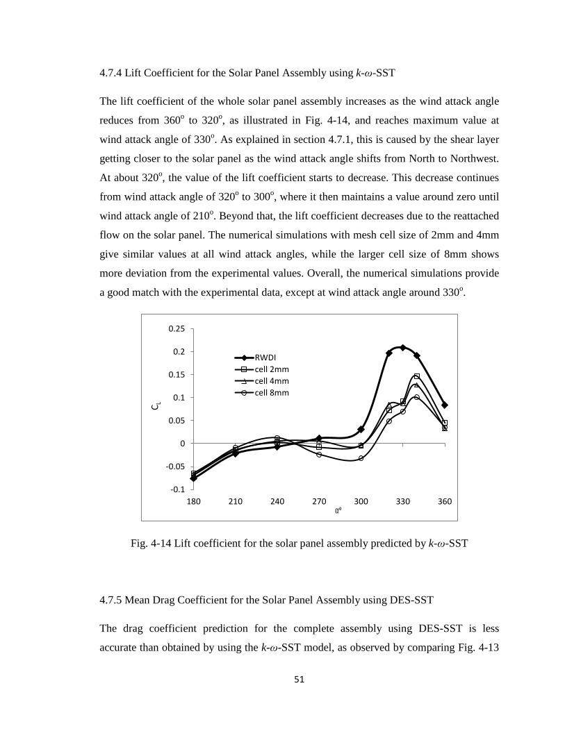
51

4.7.4 Lift Coefficient for the Solar Panel Assembly using k-ω-SST

The lift coefficient of the whole solar panel assembly increases as the wind attack angle

reduces from 360o to 320o, as illustrated in Fig. 4-14, and reaches maximum value at

wind attack angle of 330o. As explained in section 4.7.1, this is caused by the shear layer

getting closer to the solar panel as the wind attack angle shifts from North to Northwest.

At about 320o, the value of the lift coefficient starts to decrease. This decrease continues

from wind attack angle of 320o to 300o, where it then maintains a value around zero until

wind attack angle of 210o. Beyond that, the lift coefficient decreases due to the reattached

flow on the solar panel. The numerical simulations with mesh cell size of 2mm and 4mm

give similar values at all wind attack angles, while the larger cell size of 8mm shows

more deviation from the experimental values. Overall, the numerical simulations provide

a good match with the experimental data, except at wind attack angle around 330o.

Fig. 4-14 Lift coefficient for the solar panel assembly predicted by k-ω-SST

4.7.5 Mean Drag Coefficient for the Solar Panel Assembly using DES-SST

The drag coefficient prediction for the complete assembly using DES-SST is less

accurate than obtained by using the k-ω-SST model, as observed by comparing Fig. 4-13

-0.1

-0.05

0

0.05

0.1

0.15

0.2

0.25

180 210 240 270 300 330 360


C L

52

and Fig. 4-15. The predicted mean drag coefficient is in good agreement with the

experimental values for most wind attack angles, except at wind attack angles in the

range of 320o and 360o. This is likely due to the fact that the 8mm size mesh may be too

coarse for accurate simulation using the DES-SST model over the complete range of

wind directions.

Fig. 4-15 Mean drag coefficient for the solar panel assembly predicted by DES-SST

(with coarse mesh)

4.7.6 Mean Lift Coefficient for the Solar Panel Assembly using DES-SST

The mean lift coefficient prediction for DES-SST is also less accurate compared with the

prediction from k-ω-SST model, as seen from a comparison of Fig. 4-14 and Fig. 4-16. It

is clear from Fig. 4-15 and Fig. 4-16 that the drag is easier to predict with DES-SST than

the lift. It is also evident that the 8mm mesh is too coarse for an accurate DES-SST

simulation.

-0.1

-0.05

0

0.05

0.1

0.15

180 210 240 270 300 330 360

RWDI

cell 8mmC D

αo

53

Fig. 4-16 Mean lift coefficient for the solar panel assembly predicted by DES

(with coarse mesh)

4.7.7 Peak Drag Coefficient for the Solar Panel Assembly using DES-SST

The prediction of peak drag coefficient has a good match with experimental data except

at wind attack angle of 240o (see Fig. 4-17). The peak drag coefficient is caused by

fluctuations of the wind load. The deviation from experimental data is likely the result of

two main factors; one is that the mesh is too coarse, the second is that the turbulence

model itself may not accurately represent the complicated flow phenomena in the vicinity

of the solar panel assembly.

-0.1

-0.05

0

0.05

0.1

0.15

0.2

0.25

180 210 240 270 300 330 360

RWDI

cell 8mm

C L

αo

54

Fig. 4-17 Peak drag coefficient for the solar panel assembly predicted by DES

(with coarse mesh)

4.7.8 Peak Lift Coefficient for the Solar Panel Assembly using DES-SST

The prediction of the peak lift coefficient does not agree with the experimental results,

although the model does predict the correct trend of the peak lifting force, as seen in Fig.

4-18. The reasons for these inaccuracies are similar with prediction of the peak drag, as

explained above.

Fig. 4-18 Peak lift coefficient for the solar panel assembly predicted by DES

(with coarse mesh)

0.6

0.8

1

1.2

1.4

1.6

1.8

180 210 240 270 300 330 360

RWDI

cell 8mm

Peak

CD

αo

0

0.1

0.2

0.3

0.4

0.5

0.6

0.7

0.8

180 210 240 270 300 330 360

RWDI

cell 8mm

Peak

CL

αo

55


Even though there is no uncertainty analysis about wind tunnel test result, and the test

results should be viewed with some trepidation, we still can draw some conclusions from

the current study.

For drag coefficient prediction, the numerical simulation from k-ω-SST has a good match

with the experimental data at most wind attack angles, with three levels of cell fineness.

However, for lift coefficient, the simulation is not as good. The numerical simulation

results from cell sizes of 2mm and 4mm are similar, and closer to the experimental data

when compared with the results from the 8mm cell mesh, and the numerical simulation

has a good match with experimental data at all wind attack angles except 330o. There are

couple reasons why this occurs. First, the uncertainty level of the wind tunnel test results,

which has not been reported, is unknown. Second, one can question whether the number

of pressure taps used in the experiments are enough for capturing the essential flow

features (a total of six pressure taps for one solar panel, four in the top surface and two in

the bottom surface). Third, the quality of tetrahedral mesh may not be adequate enough to

ensure accurate simulation results. Finally, the capability of the turbulence model to

capture the key turbulence characteristics of this flow has to be considered.

DES did not improve the simulation results for the mean wind load compare with those

from k-ω-SST. The prediction of the peak drag matches well with experimental data,

except at wind attack angle of 240o, and the prediction of peak drag is much better than

the peak lift.

56

CHAPTER 5

Mean Wind Load on Roof Mounted Solar Panel Arrays in an

Atmospheric Boundary Layer (Other Configurations)

The solar panel basic case simulations performed in Chapter 4 have shown that both k-ω-

SST and DES-SST adequately predict the mean lift and drag coefficients at most wind

attack angles, and the maximum peak wind load from the DES-SST model occurs at

approximately the same location as the maximum mean wind load (around 330o).

Therefore, in this chapter, the k-ω-SST model is used to investigate wind load changes if

the configuration of the solar panel assembly is altered. Three configurations are

investigated: i) the solar panel lateral space is increased from 0.125 inches to 2.5 inches

(Case 1), ii) the solar panel vertical distance off the roof is increased by 6 inches (Case 2),

and iii) the vertical space between the solar panel and the roof is increased to the same

height (2.5 feet) as an installed parapet (Case 3).

The computational domain, boundary conditions and the numerical setup are the same as

in the basic case in Chapter 4. The mesh used for both Case 1 and Case 2 has cell size of

2 mm near the solar panel, with a total number of cells reaching around 1 million. For

Case 3, the simulations are carried out on a mesh with 6mm cell size near the solar panel

and parapet, with a total cell number of around 0.7 million.


5.1.1 Drag Coefficient for the Solar Panel Assembly

The effects of the modified configurations described above on the drag coefficient are

illustrated in Fig. 5-1.

a). (Case 1) Increase of the lateral space

As seen in Fig 5-1, increasing the solar panel lateral space by 2.5 inches does not change

the drag at most wind attack angles, except at angles between 360o to 330o, where the

drag shows a mild increase.

57

b). (Case 2) Increase of the vertical space off the roof

Increasing the vertical space between the solar panel and the roof significantly increases

the drag at wind attack angles of 360o to 300o, while there is negligible or no increase for

the remaining wind attack angles. This is due to the fact that an increase in the vertical

space causes more flow to directly impinge on the wind deflector, which subsequently

increases the drag. Figure 5-2 shows the velocity vectors around the assembly at wind

attack angle of 330o.

c). (Case 3) Increase of the vertical space to the same height as a parapet

Increasing the vertical spacing of the solar panel off the roof to the same level of the

parapet has a similar effect as Case 2. However, at wind attack angles from 360o to 320o,

the drag is slightly lower than in Case 2, while at wind attack angles from 270o to 180o,

the drag is a little higher than Case 2. The reason is same as in Case 2. Figure 5-3

illustrates the velocity vectors around the panel assembly and parapet at wind attack angle

of 330o.

Fig. 5-1 Drag coefficient for three configurations of the solar panel assembly

-0.05

0

0.05

0.1

0.15

0.2

0.25

0.3

180 210 240 270 300 330 360

basic casecase 1case 2case 3

C D

αo

58

Fig. 5-2 Velocity vector field at wind attack angle of 330o for vertical spacing of 6 inches

off the roof

Fig. 5-3 Velocity vector field at wind attack angle of 330o for vertical spacing at same

height as the parapet

5.1.2 Lift Coefficient for the Solar Panel Assembly

The effects of the modified configurations described above on the lift coefficient are

illustrated in Fig. 5-4.

a). (Case 1) Increase of the lateral space

Increasing the solar panel lateral space reduces the lift force significantly at wind attack

angles between 360o to 320o, while at the remaining wind attack angles, the effect is mild.

The reason for this may be that the pressure difference between the top surface and

59

bottom surface of both the solar panel and wind deflector decreases due to the ventilation

between them.

b). (Case 2) Increase of the vertical space between the solar panel and roof

Increasing the vertical space between the solar panel and roof has a similar effect on the

lift force as increasing the solar panel lateral space. It significantly reduces the lift force

for wind attack angles between 360o to 300o, while the effect on lift is minimal at the

remaining wind attack angles. Since an increase in vertical spacing causes more flow to

directly impinge on the wind deflector, this direct impact increases the drag force and at

the same time produces more downward force (reducing the lift force), consistent with

the velocity field for wind attack angle of 330o seen in Fig. 5-2.

c). (Case 3) Increase of the vertical space between the solar panel and roof to the same

height as a parapet

Increasing the vertical space between the solar panel and the roof to the same level as a

parapet reduces the lift force significantly at wind attack angles between 360o to 270o.

The same amount of lift force is maintained at wind attack angles from 270o to 240o, and

the lift force increases significantly at wind attack angles from 240o to 180o. The increase

in vertical space to the same level as the parapet causes more flow to directly impact on

the wind deflector and more flow reattaches onto the solar panel, subsequently causing an

increase in drag and a reduction in lift force on the assembly. The velocity vectors for this

case at wind attack angle of 330o are shown in Fig. 5-3. At a wind attack angle of 210o,

the flow is shielded by the parapet and the lift coefficient increases due to a recirculation

flow that develops near the parapet, as seen in Fig. 5-5.

60

Fig. 5-4 Lift coefficient for three configurations of the solar panel assembly

Fig. 5-5 Velocity vectors at wind attack angle of 210o for vertical spacing at the same

height as the parapet

5.2 Conclusions

Using the k-ω-SST model with the same setup as the basic case, results have been

obtained for three modified cases. Increasing the solar panel lateral spacing by 2.5 inches

does not increase the drag at most wind attack angles, except between wind attack angles

of 360o and 330o, where there is a mild drag increase. However, it will significantly

-0.25

-0.2

-0.15

-0.1

-0.05

0

0.05

0.1

0.15

0.2

180 210 240 270 300 330 360

basic case

case 1

case 2

case 3C L

αo

61

reduce the wind lift force between 360o and 320o. Increasing the solar panel vertical

spacing off the roof by 6 inches increases the drag dramatically for wind attack angles

from 360o to 300o, while it greatly reduces the lift force at these wind attack angles.

Installing the solar panel at the same height above the roof as a parapet increases the drag

significantly at wind attack angles from 360o to 300o, reduces the lift force for wind

attack angles from 360o to 270o and increases the lift force for 240o to 180o wind attack

angles.

62

CHAPTER 6

Conclusions and Future Work

6.1 Conclusions

In this thesis, the flow over a cube in an atmospheric boundary has been simulated using

different computational domains with the k-ω-SST turbulence model, and the most

computationally economic domain size has been identified. With this domain size, seven

RANS models, DES-SST and LES models have been tested to predict the pressure

coefficient (Cp) distribution. From comparison of simulation results with experimental

data, it was determined that the k-ω-SST and Reynolds Stress models give the best

prediction of pressure coefficient distribution on the vertical symmetrical plane, closely

matching with experimental data. The Spalart-Allmaras model, k-ε RNG and k-ε

Realizable models give reasonably good prediction, while the k-ε standard and k-ω

standard failed to predict the pressure coefficient distribution, especially on the roof and

windward face. Neither the DES-SST model nor the LES model with dynamic

Smagorinksy option gives better prediction of Cp, contrary to expectations. The reason

for this may be that the mesh is not fine enough close to the wall. The flow patterns

predicted by each model look similar at first sight, except for the k-ε standard and k-ω

standard, which fail to predict the rooftop flow separation bubble. However, when closely

scrutinized, these flow patterns exhibit some differences. In particular, the wake region

recirculation length predicted by the RANS models is longer than that from the DES-SST

and LES models, which is consistent with information reported in the literature.

The Cp difference across a canopy in an atmospheric boundary layer has also been

predicted with the above-mentioned models. Two levels of mesh fineness have been

implemented. No model shows superior prediction performance, but k-ω-SST

demonstrates relatively better prediction. Compared with the coarse mesh results, fine

mesh does improve the simulation results for all the RANS models at some wind attack

angles. The largest deviation from experimental data for the k-ω-SST model is at a wind

attack angle of 150o, which is around 30%. With the coarse mesh, the Cp difference has

been predicted using DES-SST and the LES model with Smagorinksy option. Either

63

model gives both mean and peak wind load. However, they do not demonstrate better

prediction of mean wind load than the k-ω-SST model. LES gives relatively better

prediction in Cp difference than the DES-SST model, but it requires more computing

power.

After simulation of the flow past a cube and the canopy flow with different models, the k-

ω-SST and DES-SST models have been selected to conduct simulation of the wind load

on roof mounted solar panels. Wind load on one of 16 solar panels in the corner of the

roof of a building is tracked. For the k-ω-SST model, three levels mesh fineness have

been used, while the coarsest mesh is used for the DES-SST. Simulation results show that

with the finest mesh, k-ω-SST can accurately predict the Cp difference on solar panels at

all wind attack angles except near 330o, while it gives a more accurate prediction for the

wind deflector at all wind attack angles. In terms of drag coefficient and lift coefficient

on the assembly, k-ω-SST gives more accurate prediction of drag than of lift. Compared

with the k-ω-SST model, DES-SST gives a less accurate prediction of both drag

coefficient and lift coefficient. The peak load prediction from DES-SST is good for drag

but not so good for lift when compared with experimental data. Both the DES-SST model

and experimental results show similar mean and peak wind load trends vs. wind attack

angle, which indicates that the mean wind load has a close relation with the peak wind

load.

Based on the close relationship of the mean and peak wind load, we use the k-ω-SST

model to disclose the wind load change with three different configurations, increasing the

lateral space from 0.125 inches to 2.5 inches (Case1), increasing the vertical space from 1

inch to 6 inches (Case 2), increasing the vertical space to the same height as a parapet

(Case 3). The simulations for Case 1 show that there is no drag change for most wind

attack angles except in the 360o to 330o range. However, it will significantly reduce the

wind lift force between 360o and 320o. For Case 2, the drag dramatically increases for

wind attack angles from 360o to 300o, while the lift force is greatly reduced at these wind

attack angles. For case 3, the drag increases significantly at wind attack angles from 360o

to 300o, while the lift force reduces for wind attack angles from 360o to 270o and

increases for 240o to 180o wind attack angles.

64

6.2 Future Work

On the basis of the analysis provided in this thesis, it is recommended that the mesh near

the walls and solar panel surfaces be refined to better predict the wind load using the k-ω-

SST, DES-SST and LES models. Tracking more solar panels near the roof corner will

give more information about wind load on solar panels. Finally, carefully conducted

experiments are warranted to provide more detailed data which can be used to validate

the CFD models.

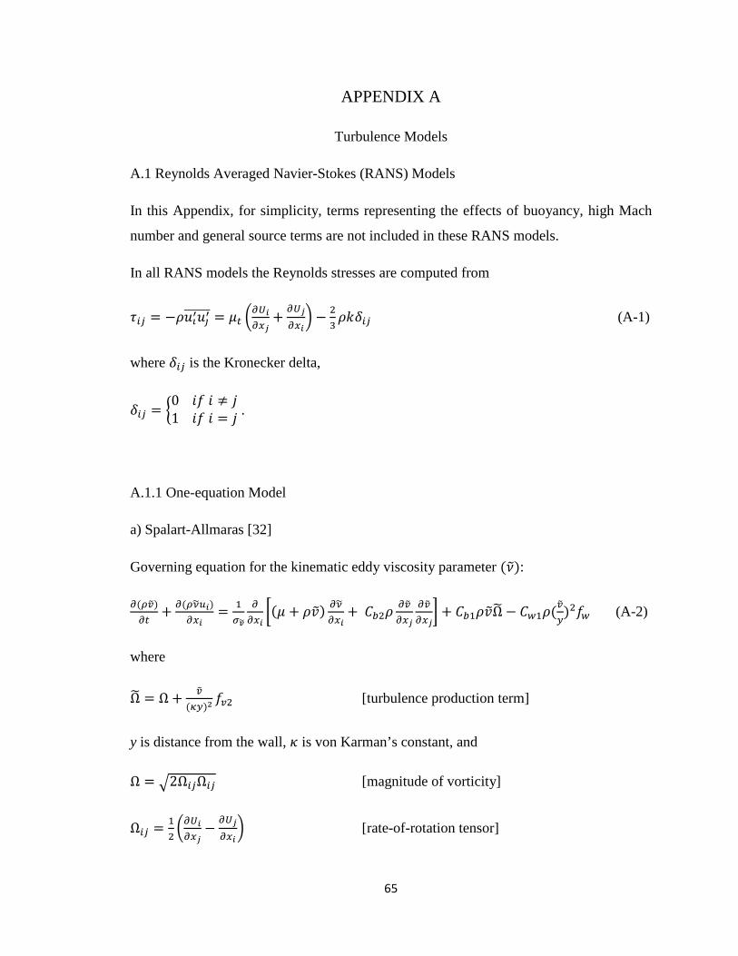
65

APPENDIX A

Turbulence Models

A.1 Reynolds Averaged Navier-Stokes (RANS) Models

In this Appendix, for simplicity, terms representing the effects of buoyancy, high Mach

number and general source terms are not included in these RANS models.

In all RANS models the Reynolds stresses are computed from

𝜏𝑖𝑗 = −𝜌𝑢𝚤′𝑢𝚥′�� = 𝜇𝑡 �𝜕𝑈𝑖𝜕𝑥𝑗

+ 𝜕𝑈𝑗𝜕𝑥𝑖� − 2

3𝜌𝑘𝛿𝑖𝑗 (A-1)

where 𝛿𝑖𝑗 is the Kronecker delta,

𝛿𝑖𝑗 = �0 𝑖𝑓 𝑖 ≠ 𝑗1 𝑖𝑓 𝑖 = 𝑗 .

A.1.1 One-equation Model

a) Spalart-Allmaras [32]

Governing equation for the kinematic eddy viscosity parameter (𝜈�):

𝜕(𝜌𝑣�)𝜕𝑡

+ 𝜕(𝜌𝜈�𝑢𝑖)𝜕𝑥𝑖

= 1𝜎𝑣�

𝜕𝜕𝑥𝑖

�(𝜇 + 𝜌𝑣�) 𝜕𝜈�𝜕𝑥𝑖

+ 𝐶𝑏2𝜌𝜕𝑣�𝜕𝑥𝑗

𝜕𝑣�𝜕𝑥𝑗� + 𝐶𝑏1𝜌𝑣�Ω� − 𝐶𝑤1𝜌(𝑣�

𝑦)2𝑓𝑤 (A-2)

where

Ω� = Ω + 𝑣�(𝜅𝑦)2

𝑓𝑣2 [turbulence production term]

y is distance from the wall, 𝜅 is von Karman’s constant, and

Ω = �2Ω𝑖𝑗Ω𝑖𝑗 [magnitude of vorticity]

Ω𝑖𝑗 = 12�𝜕𝑈𝑖𝜕𝑥𝑗

− 𝜕𝑈𝑗𝜕𝑥𝑖� [rate-of-rotation tensor]

66

𝑓𝑣2 = 𝑓𝑣2 �𝑣�𝑣�, 𝑓𝑤 = 𝑓𝑤(𝑣�/(Ω�𝜅2𝑦2) [wall-damping functions]

𝐶𝑤1 =𝐶𝑏1𝑘2

+1 + 𝐶𝑏2𝜎𝑣�

𝜇𝑡 = 𝜌𝜈�𝑓𝜈1 [turbulent viscosity]

𝑓𝑣1 = 𝜒3

𝜒3+𝐶𝑣13 [viscosity damping term]

𝜒 =𝑣�𝑣

Model constants are: 𝜎𝑣� = 23

, 𝜅 = 0.4187, 𝐶𝑏1 = 0.1355, 𝐶𝑏2 = 0.622, 𝐶𝑣1 = 7.1.

Since turbulent kinetic energy is not calculated in this model, the last term in equation

(A-1) is ignored when calculating the Reynolds stresses.

A.1.2 Two-equation Models

a) k-ε standard

Governing equations for turbulent kinetic energy (k) and dissipation rate (ε):

𝜕(𝜌𝑘)𝜕𝑡

+ 𝜕(𝜌𝑘𝑢𝑖)𝜕𝑥𝑖

= 𝜕𝜕𝑥𝑖

�(𝜇 + 𝜇𝑡𝜎𝑘

) 𝜕𝑘𝜕𝑥𝑖� + 𝐺𝑘 − 𝑌𝑘 (A-3)

𝜕(𝜌𝜀)𝜕𝑡

+ 𝜕(𝜌𝜀𝑢𝑖)𝜕𝑥𝑖

= 𝜕𝜕𝑥𝑖

�(𝜇 + 𝜇𝑡𝜎𝜀

) 𝜕𝜀𝜕𝑥𝑖� + 𝐺𝜀 − 𝑌𝜀 (A-4)

where

𝐺𝑘 = 𝜇𝑡𝑆2 [kinetic energy production term]

𝐺𝜀 = 𝐶1𝜀𝜀𝑘𝐺𝑘 [kinetic energy dissipation production term]

𝑆 = �2𝑆𝑖𝑗𝑆𝑖𝑗 [modulus of strain rate tensor]

67

𝑆𝑖𝑗 = 12

(𝜕𝑢𝑖𝜕𝑥𝑗

+ 𝜕𝑢𝑗𝜕𝑥𝑖

) [strain rate tensor]

𝑌𝑘 = 𝜌𝜀 [kinetic energy destruction term]

𝑌𝜀 = 𝐶2𝜀𝜀2

𝑘 [dissipation rate destruction term]

𝜇𝑡 = 𝜌𝐶𝜇𝑘2

𝜀 [turbulent viscosity]

Model constants are: 𝐶𝜇 = 0.09, 𝜎𝑘 = 1, 𝜎𝜀 = 1.3, 𝐶1𝜀 = 1.44, 𝐶2𝜀 = 1.92.

b) k-ε RNG

Governing equations for turbulent kinetic energy (k) and dissipation rate (ε):



= 𝜕𝜕𝑥𝑗

�𝛼𝑘𝜇𝑒𝑓𝑓𝜕𝑘𝜕𝑥𝑗� + 𝐺𝑘 − 𝜌𝜀 (A-5)


+ 𝜕(𝜌𝜀𝑢𝑖)𝜕𝑥𝑖

= 𝜕𝜕𝑥𝑗

�𝛼𝜀𝜇𝑒𝑓𝑓𝜕𝜀𝜕𝑥𝑗� + 𝐶1𝜀

𝜀𝑘𝐺𝑘 − 𝐶2𝜀∗ 𝜌

𝜀2

𝑘 (A-6)

where

𝜇𝑒𝑓𝑓 = 𝜇 + 𝜇𝑡 . [effective viscosity]

The turbulent kinetic energy production term Gk is the same as in equation (A-3).

For constant 𝐶2𝜀∗ , the scale elimination procedure following RNG theory is used

𝐶2𝜀∗ = 𝐶2𝜀 +𝐶𝜇𝜂3�1−

𝜂𝜂0�

1+𝛽𝜂3 where 𝜂 = 𝑘

𝜀 �2𝑆𝑖𝑗 . 𝑆𝑖𝑗 .

Model constants are: 𝐶𝜇 = 0.0845, 𝐶1𝜀 = 1.42, 𝐶2𝜀 = 1.68, 𝜂0 = 4.377, 𝛽 = 0.012,

and

𝛼𝑘 = 𝛼𝜀 = 1.39, for high Re flow.

68

c) k-ε Realizable

Governing equation for turbulent dissipation rate (ε):


+ 𝜕(𝜌𝜀𝑢𝑗)𝜕𝑥𝑗

= 𝜕𝜕𝑥𝑗

��𝜇 + 𝜇𝑡𝜎𝜀� 𝜕𝜀𝜕𝑥𝑗� + 𝜌𝐶1𝑆𝜀 − 𝜌𝐶2

𝜀2

𝑘+√𝜈𝜀 (A-7)

where 𝑆 is modulus of the strain rate tensor defined in the k-ε standard model. The

turbulent kinetic energy transport equation is the same as equation (A-3), except that the

model constants have changed.

The turbulent viscosity is calculated following the same procedure as the k-ε standard

model, but Cµ is a variable instead of a constant,

𝐶𝜇 = 1

𝐴0+𝐴𝑠𝑘𝑈∗𝜀

where 𝑈∗ = �𝑆𝑖𝑗𝑆𝑖𝑗 + 𝛺�𝑖𝑗𝛺�𝑖𝑗

and Ω�𝑖𝑗 = Ω𝑖𝑗 − 2𝜀𝑖𝑗𝑘𝜔𝑘, Ω𝑖𝑗 = Ω𝑖𝑗 − 𝜀𝑖𝑗𝑘𝜔𝑘,

where Ω𝑖𝑗 is the mean rate-of-rotation tensor viewed in a moving reference frame with

the angular velocity of ωk and 𝜀𝑖𝑗𝑘 is the permutation tensor. In these equations,

𝐴o = 4.04, 𝐶1 = max �0.43, 𝜂𝜂+5

� , 𝜂 = 𝑆 𝑘𝜀𝜎𝜀 , 𝐴𝑠 = √6𝑐𝑜𝑠𝜙

where 𝜙 = 13

cos−1(√6𝑊), 𝑊 = 𝑆𝑖𝑗𝑆𝑗𝑘𝑆𝑘𝑖�̃�3

, �̃� = �𝑆𝑖𝑗𝑆𝑖𝑗 , 𝑆𝑖𝑗 is strain rate tensor.

Model constants are: 𝐶1𝜀 = 1.44, 𝐶2 = 1.9, 𝜎𝑘 = 1.0, 𝜎𝜀 = 1.2.

d) k-ω standard

Governing equations for turbulent kinetic energy (k) and specific dissipation rate (ω):



= 𝜕𝜕𝑥𝑗

�Γ𝑘𝜕𝑘𝜕𝑥𝑗� + 𝐺𝑘 − 𝑌𝑘 (A-8)

𝜕(𝜌𝜔)𝜕𝑡

+ 𝜕(𝜌𝜔𝑢𝑖)𝜕𝑥𝑖

= 𝜕𝜕𝑥𝑗

�Γ𝜔𝜕𝜔𝜕𝑥𝑗� + 𝐺𝜔 − 𝑌𝜔 (A-9)

69

where Gk and 𝑌𝑘 are kinetic energy production and destruction terms, respectively.

and Gk is identical to that of governing equations of k-ε and its variants

Γ𝑘 = 𝜇 +𝜇𝑡𝜎𝑘

, Γ𝜔 = 𝜇 +𝜇𝑡𝜎𝜔

𝜇𝑡 = 𝛼∗ 𝜌𝑘𝜔

[turbulent viscosity for a low Re]

𝛼∗ = 𝛼∞∗ �𝛼0+∗

𝑅𝑒𝑡𝑅𝑘

1+𝑅𝑒𝑡𝑅𝑘

�

𝑅𝑒𝑡 = 𝜌𝑘𝜇𝜔

, 𝑅𝑘 = 6.0, 𝛼0∗ = 𝛽𝑖3

, 𝛽𝑖 = 0.072.

At high Reynolds number, 𝛼∗and 𝛼∞∗ are both taken to be 1.

𝐺𝜔 = 𝛼 𝜔𝑘𝐺𝑘 [specific dissipation rate production term]

𝛼 =𝛼∞𝛼∗

�𝛼0 + 𝑅𝑒𝑡

𝑅𝜔1 + 𝑅𝑒𝑡

𝑅𝜔

�

where 𝑅𝜔 = 2.95, α* and Ret are defined as above.

For high Re, 𝛼 and 𝛼∞ are both taken to be 1.

𝑌𝑘 = 𝜌𝛽∗𝑓𝛽∗𝑘𝜔 [kinetic energy destruction term]

where 𝑓𝛽∗ = 1+680𝑥𝑘2

1+400𝑥𝑘2 with

𝑥𝑘 = �1 𝑖𝑓 𝑥𝑘 > 01𝜔3

𝜕𝑘𝜕𝑥𝑗

𝜕𝜔𝜕𝑥𝑗

𝑖𝑓𝑥𝑘 ≤ 0 ,

𝛽∗ = 𝛽𝑖∗[1 + 𝜁∗𝐹(𝑀𝑡)] , where 𝜁∗ = 1.5 and 𝐹(𝑀𝑡) = 0 when in low Mach number

flow, and

70

𝛽𝑖∗ = 𝛽∞∗

⎝

⎜⎛

415 + �𝑅𝑒𝑡𝑅𝛽

�4

1 + �𝑅𝑒𝑡𝑅𝛽�4

⎠

⎟⎞

where 𝑅𝛽 = 8.0, 𝛽∞∗ = 0.09 and 𝑅𝑒𝑡 is calculated as above.

𝑌𝜔 = 𝜌𝛽𝑓𝛽𝜔2 [specific dissipation rate destruction term]

where 𝛽 is related to fluid Mach number, when in low Mach number, 𝛽 = 𝛽𝑖

𝑓𝛽 =1 + 70𝑥𝜔1 + 80𝑥𝜔

𝑥𝜔 = �Ω𝑖𝑗Ω𝑗𝑘S𝑘𝑖(𝛽∞∗ 𝜔)3 �

where Ski and Ω𝑖𝑗 are the strain rate tensor and rotation rate tensor, respectively. They are

calculated the same way as in the Spalart-Allmaras model and k-ε standard model.

For incompressible flow and high Re,

𝛽∗ = 𝛽𝑖∗, 𝛽𝑖∗ = 𝛽∞∗ .

Model constants are: 𝜎𝑘 = 2.0, 𝜎𝜔 = 2.0, 𝛼∞∗ = 1, 𝛼∞ = 0.52, 𝛼0 = 19

, 𝛽∞∗ = 0.09,

𝛽𝑖 = 0.072, 𝑅𝛽 = 8.0, 𝑅𝑘 = 6.0, 𝑅𝜔 = 2.95, 𝑀𝑡𝑜 = 0.25.

e) k-ω-SST

Governing equations for turbulent kinetic energy (k) and specific dissipation rate (ω):



= 𝜕𝜕𝑥𝑗

�Γ𝑘𝜕𝑘𝜕𝑥𝑗� + 𝐺�𝑘 − 𝑌𝑘 (A-10)

𝜕(𝜌𝜔)𝜕𝑡


= 𝜕𝜕𝑥𝑗

�𝛤𝜔𝜕𝑘𝜕𝑥𝑗� + 𝐺𝜔 − 𝑌𝜔 + 𝐷𝜔 (A-11)

71

Both diffusion coefficients Γ𝑘 and Γ𝜔 have the same form of those in k-ω standard model,

but the turbulent viscosity is computed from

𝜇𝑡 = 𝜌𝑘𝜔

1

𝑚𝑎𝑥� 1𝑎∗,𝑆𝐹2𝑎1𝜔� ,

where S is modulus of the strain rate tensor, and

𝜎𝑘 = 1𝐹1𝜎𝑘,1

+(1−𝐹1)𝜎𝑘,2

[Prandtl number]

𝜎𝜔 = 1𝐹1𝜎𝜔,1

+(1−𝐹1)𝜎𝜔,2

[Prandtl number]

𝑎∗ is a damping factor which is the same as in the k-ω standard model, and 𝐹1 , 𝐹2 are

blending functions.

𝐺𝜔 = 𝛼𝜈𝑡𝐺�𝑘, [production of specific dissipation rate]

𝐺�𝑘 = min(𝐺𝑘, 10𝜌𝛽∗𝑘𝜔) [production of kinetic energy]

𝛼 takes the same form as in the k-ω standard model, however 𝛼∞ in that model is

constant, while here it is variable, given by

𝛼∞ = 𝐹1𝛼∞,1 + (1 − 𝐹1)𝛼∞,2

where 𝛼∞,1 = 𝛽𝑖,1𝛽∞∗

− 𝜅12

𝜎𝜔,1�𝛽∞∗ , 𝛼∞,2 = 𝛽𝑖,2

𝛽∞∗− 𝜅12

𝜎𝜔,2�𝛽∞∗, and κ1 = 0.41.

In equations (A-10) and (A-11), the dissipation terms are defined as

𝑌𝑘 = 𝜌𝛽∗𝑘𝜔 [dissipation of k]

where 𝛽∗ is the same as in the k-ω standard model, and

𝑌𝜔 = 𝜌𝛽𝜔2 [dissipation of ω]

where 𝛽 is the same as in the k-ω standard model, in the equation of 𝛽, 𝛽i is obtained

from

72

𝛽𝑖 = 𝐹1𝛽𝑖,1 + (1 − 𝐹1)𝛽𝑖,2

𝐷𝜔 = 2(1 − 𝐹1)𝜌 1𝜔𝜎𝜔,2

𝜕𝑘𝜕𝑥𝑗

𝜕𝜔𝜕𝑥𝑗

, [cross-diffusion modification]

Model constants are: 𝜎𝑘 = 1.0, 𝜎𝜔,1 = 2.0, 𝜎𝜔,2 = 1.17, 𝛽∗ = 0.09, 𝛽𝑖,1 = 0.075,

𝛽𝑖,2 = 0.0828.

A.1.3 Reynolds Stress Model

Governing equations for the Reynolds stresses 𝑢𝚤′𝑢𝚥′�� (i,j = 1,2,3) are:

𝜕𝜕𝑡

(𝜌𝑢𝚤′𝑢𝚥′��) + 𝐶𝑖𝑗 = 𝑃𝑖𝑗 + 𝐷𝑖𝑗 − 𝜀𝑖𝑗 + Φ𝑖𝑗 + Ω𝑖𝑗 (A-12)

In these equations,

𝐶𝑖𝑗 = 𝜕𝜕𝑥𝑘

(𝜌𝑢𝑘𝑢𝚤′𝑢𝚥′��) [convection term of Reynolds stress transport]

𝑃𝑖𝑗 = −𝜌(𝑢𝚤′𝑢𝑘′�� 𝜕𝑈𝑗𝜕𝑥𝑘

+ 𝑢𝚥′𝑢𝑘′�� 𝜕𝑈𝑖𝜕𝑥𝑘

) [production term of Reynolds stress transport]

Ω𝑖𝑗 = −2𝜌Ω𝑘(𝑢𝚥′𝑢𝑚′��𝑒𝑖𝑘𝑚 + 𝑢𝚤′𝑢𝑚′��𝑒𝑗𝑘𝑚), [rotation term of Reynolds stress transport]

where ωk is the rotation vector; eijk equals 1 if i, j, k are different and in cyclic order,

equals -1 if indices are in anti-cyclic order, and equals zero if two indices are the same.

𝐷𝑖𝑗 = 𝜕𝜕𝑥𝑘

(𝜇𝑡𝜎𝑘

𝜕𝑢𝚤′𝑢𝚥′��

𝜕𝑥𝑘) [diffusion term of Reynolds stress transport]

where σk = 0.82 and

𝜇𝑡 = 𝜌𝐶𝜇𝑘2

𝜀 , with Cµ = 0.09, and

𝜀𝑖𝑗 = 23𝜀𝛿𝑖𝑗 [dissipation term of Reynolds stress transport]

where 𝛿𝑖𝑗 is the Kronecker delta.

73

𝛷𝑖𝑗 = 𝑝 �𝜕𝑢𝚤′

𝜕𝑥𝚥+

𝜕𝑢𝚥′

𝜕𝑥𝚤�

�� [pressure strain term of Reynolds stress transport]

In the classic approach, the pressure strain term is decomposed into three components

𝜙𝑖𝑗 = 𝜙𝑖𝑗,1 + 𝜙𝑖𝑗,2 + 𝜙𝑖𝑗,𝑤

where

𝜙𝑖𝑗,1 = −𝐶1𝜌𝜀𝑘�𝑢𝚤′𝑢𝚥′�� − 2

3𝛿𝑖𝑗𝑘� [slow pressure-strain term]

𝜙𝑖𝑗,2 = −𝐶2[�𝑃𝑖𝑗 + 𝐹𝑖𝑗 + 5𝐺𝑖𝑗/6 − 𝐶𝑖𝑗� −13𝛿𝑖𝑗(𝑃𝑘𝑘 + 5𝐺𝑘𝑘/6 − 𝐶𝑘𝑘)]

[rapid pressure-strain term]

𝜙𝑖𝑗,𝑤 = 𝐶1′𝜀𝑘�𝑢𝑘′ 𝑢𝑚′��𝑛𝑘𝑛𝑚𝛿𝑖𝑗 −

32𝑢𝚤′𝑢𝑘′��𝑛𝑗𝑛𝑘 −

32𝑢𝚥′𝑢𝑘′��𝑛𝑖𝑛𝑘�

𝐶𝑙𝑘32

𝜀𝑑

+𝐶21(𝜙𝑘𝑚,2𝑛𝑘𝑛𝑚𝛿𝑖𝑗 −32𝜙𝑖𝑘,2𝑛𝑗𝑛𝑘 −

32𝜙𝑗𝑘,2𝑛𝑖𝑛𝑘) 𝐶𝑙𝑘

32

𝜀𝑑 [wall reflection term]

where 𝐶1 = 1.8, 𝐶2 = 0.6, 𝐶1′ = 0.5, 𝐶2′ = 0.3, and

𝑛𝑘 is the 𝑥𝑘 component of the unit normal to the wall, d is the distance to the wall, and

𝐶𝑙 =𝐶𝜇3/4

𝜅 , with κ = 0.4187 and 𝐶𝜇 = 0.09.

The scalar dissipation rate ε is modeled similar with the k-ε standard model.

A.2 Large Eddy Simulation (LES)

Based on the Boussinesq hypothesis, the subgrid stresses are calculated from:

𝜏𝑖𝑗 = −2𝜇𝑆𝐺𝑆𝑆�̅�𝑗 + 13𝜏𝑘𝑘𝛿𝑖𝑗 (A-13)

where 𝜇𝑆𝐺𝑆 = 𝜌𝐿𝑠2�2𝑆�̅�𝑗𝑆�̅�𝑗, [subgrid viscosity]

74

𝑆�̅�𝑗 = 12

(𝜕𝑢�𝑖𝜕𝑥𝑗

+ 𝜕𝑢�𝑗𝜕𝑥𝑖

), [strain rate tensor for resolved scale]

𝐿𝑠 = min (𝜅𝑑,𝐶𝑠Δ) [mixing length for subgrid scales]

κ is the von Karman constant, d is distance to the closest wall and 𝐶𝑠 is the Smagorinsky

constant, which is not a universal constant.

Δ = 𝑉1/3 [local grid scale]

where V is computational cell volume.

In equation (A-13), the 𝜏𝑘𝑘 subgrid-scale stresses are not modeled. For incompressible

flow, terms involving 𝜏𝑘𝑘 can be added to the filtered pressure or simply neglected.

The dynamic subgrid-scale (SGS) model proposed by Germano et al. [7] determines the

SGS stress difference with two different filtering operations with cutoff widths ∆1 and ∆2,

𝜏𝑖𝑗(2) − 𝜏𝑖𝑗

(1) = 𝜌𝑢�𝚤𝑢�𝚥�� − 𝜌𝑢�𝑖𝑢�𝑗 (A-14)

where the bracketed superscripts (1) and (2) indicating filtering at cutoff widths ∆1 and

∆2, respectively.

In the case of bluff body flows, Germano’s SGS model usually gives better simulation

results [22]. This option is used in the current research.

Large Eddy Simulation (LES) needs much more computing power than RANS models,

but it gives more accurate results in the case of bluff body flows.

A.3 Detached Eddy Simulation (DES)

In the Detached Eddy Simulation (DES) approach, the unsteady RANS models are

employed in the boundary layer and LES is applied in the separated regions. DES models

have been specially designed to address high Reynolds number wall bounded flows,

where the cost of computation is very high when using LES. The computational cost for

DES is lower than LES but is higher than RANS. Fluent offers three types of RANS

75

model for DES, the Spalart-Allmaras model, the k-ε Realizable model and the k-ω-SST

model.

In the current research, the k-ω-SST based DES proposed by Menter et al. [20], has been

used.

The kinetic energy dissipation term in the transport equation is imbedded into the DES

model through the following formula:

𝑌𝑘 = 𝜌𝛽∗𝑘𝜔𝐹𝐷𝐸𝑆

where 𝐹𝐷𝐸𝑆 = max ( 𝐿𝑡𝐶𝑑𝑒𝑠∆𝑚𝑎𝑥

, 1) , 𝐶𝑑𝑒𝑠 = 0.61 , ∆𝑚𝑎𝑥 is maximum of the local grid

spacing ∆𝑥, ∆𝑦, ∆𝑧 and

𝐿𝑡 = √𝑘𝛽∗𝜔

[turbulent length scale]

which is used to define the RANS model, where k is turbulent kinetic energy, 𝜔 is

specific dissipation rate and 𝛽∗ = 0.09 for high Reynolds number incompressible flow.

76

APPENDIX B

Near-Wall Treatment

The presence of a wall not only greatly changes the mean flow to satisfy the no-slip

condition, but also dramatically influences the turbulent characteristics near the wall.

Near the wall, the mean velocity experiences a large gradient, and the fluctuations of the

flow in all three directions reduce from their peak value to zero at the wall surface due to

the damping effect of the wall. Among the three components, the streamwise fluctuation

has the highest peak value near the wall.

Numerous experiments demonstrate that the near-wall flow region can be subdivided into

three layers; the viscous layer, the buffer layer and the outer layer. Inside the viscous

layer, also called the laminar layer, the viscous force plays the dominant role. In the outer

layer, the turbulent Reynolds stresses have a major role, while in the buffer layer, both

viscous and turbulence forces share an equal role.

Traditionally, there are two approaches to model the near-wall flow region. One approach

is to use the “standard wall function”, which uses an empirical equation to “bridge” the

viscous layer to the outer layer, and the viscous region is not resolved [3]. This approach

saves computing cost, but the accuracy of the solution gets worse once the y* value

reaches 15, when the mesh near the wall gets refined. Another approach is to use a wall

model near the wall [3], so the flow inside the three layers all get resolved. The mesh near

the viscous layer is usually very fine in this case.

B.1 Standard Wall Function

The law-of-the-wall for mean velocity is

𝑈∗ = 1𝜅

ln (𝐸𝑦∗) (B-1)

where 𝑈∗ =𝑈𝑝𝐶𝜇

1/4𝑘𝑝1/2

𝜏𝑤/𝜌

and 𝑦∗ =𝜌𝐶𝜇

1/4𝑘𝑝1/2𝑦𝑝

𝜇 .

77

Here 𝜅 is the von Karman constant, equal to 0.4187, E = 0.793, 𝑈𝑝 is the mean velocity at

the near wall node P, kp is turbulent kinetic energy at node P, yp is the distance from the

wall to the node P and 𝜇 is the dynamic viscosity of the fluid. The y* value should be of

the order of 15 at the low end, and the high end value depends on the Reynolds number of

the flow.

In Fluent, once y* > 11, the log-law is employed. When y* < 11, the laminar strain-stress

relationship is used,

U* = y*.

B.2 Scalable Wall Functions

In Fluent, a scalable wall function has been introduced to avoid solution deterioration

when y* < 11 for a refined mesh. For y* > 11, the scalable wall function is identical to the

standard wall function. When y* < 11, a limiter is introduced,

𝑦�∗ = max(𝑦∗,𝑦𝑙𝑖𝑚𝑖𝑡∗ ), where 𝑦𝑙𝑖𝑚𝑖𝑡∗ = 11.

B.3 Enhanced Wall Treatment

Fluent combines the two-layer model with the so-called “enhanced wall function”, in

order to reach the goal of obtaining the accuracy of the two-layer model when 𝑦+ ≈

1, and not significantly reducing the accuracy of the standard wall function meshes. In

this approach, the whole computation domain is subdivided into a viscosity-affected

region and a fully-turbulent region. The demarcation of the two regions is determined by

a wall distance-based turbulent Reynolds number, Rey, which is defined as

𝑅𝑒𝑦 = 𝜌𝑦√𝑘𝜇

,

where y is the normal distance from the wall.

78

When 𝑅𝑒𝑦 > 𝑅𝑒𝑦∗ , where 𝑅𝑒𝑦∗ = 200, the k-ε or RSM is activated, when 𝑅𝑒𝑦 < 𝑅𝑒𝑦∗ , the

one-equation model of Wolfstein [3] is activated.

The law-of-the-wall has been modified as a single wall law for the entire wall region,

𝑢+ = 𝑒Γ𝑢𝑙𝑎𝑚+ + 𝑒1Γ𝑢𝑡𝑢𝑟𝑏+ , (B-2)

where the blending function Γ = −𝑎(𝑦+)4

1+𝑏𝑦+

and a = 0.01, b = 5.

𝑑𝑢+

𝑑𝑦+= 𝑒Γ 𝑑𝑢𝑙𝑎𝑚

+

𝑑𝑦++ 𝑒

1Γ𝑑𝑢𝑡𝑢𝑟𝑏

+

𝑑𝑦+

B.4 LES Near-Wall Treatment

When the mesh is fine enough to resolve the laminar sublayer, the wall shear stress is

obtained from the laminar stress-strain relationship,

𝑢�𝑢𝜏

= 𝜌𝑢𝜏𝑦𝜇

.

If the mesh is very coarse, then the law-of-the-wall is applied,

𝑢�𝑢𝜏

= 1𝜅𝑙𝑛𝐸(𝜌𝑢𝜏

𝜇).

If the first near-wall point lies in the buffer region, equation (B-2) can be used.

Another approach is to use the Werner and Wengle wall function [36]. When the cells at

the wall are not very fine, the following wall function can give better simulation results

than the two-layer wall model [3],

|𝜏𝑤| = 2𝜇�𝑢𝑝�Δ𝑧

, for �𝑢𝑝� ≤𝜇

2𝜌∆𝑧𝐴

21−𝐵 (B-3)

|𝜏𝑤| = 𝜌 �1−𝐵2𝐴1+𝐵1−𝐵( 𝜇

𝜌∆𝑧)1+𝐵 + 1+𝐵

𝐴( 𝜇𝜌∆𝑧

)𝐵�𝑢𝑝��2

1+𝐵, for �𝑢𝑝� ≥

𝜇2𝜌∆𝑧

𝐴2

1−𝐵

79

REFERENCES

[1] Adrian, R., Steady Wind Pressures on Solar Collectors on Flat-Roofed Buildings. J. of

Wind Eng. and Ind. Aerodyn., Vol. 23(1), pp. 249-258, 1985.

[2] Adrian, R., Wind Forces on Structures Supporting Solar Collectors. J. of Wind Eng.

and Ind. Aerodyn., Vol. 32(1), pp. 93-100, 1989.

[3] ANSYS Theory Guide, Release 13.0, pp. 121-122, 2010.

[4] ASCE 7-05 Minimum Design Loads for Buildings and Other Structures, American

Society of Civel Engineers, Jan, 2006, ISBN: 0784408092.

[5] Bronkhorst, A., Franke, J., Geurts, C., Bentum, C.V. and Grepinet, F., Wind Tunnel

and CFD Modelling of Wind Pressures on Solar Energy Systems on Flat Roofs. The Fifth

International Symposium on Computational Wind Engineering (CWE2010), Chapel Hill,

North Carolina, USA, May 23-27, 2010.

[6] Franke, J., Hellsten, A., Schlünzen, H. and Carissimo, B., Best Practice Guideline for

the CFD Simulation of Flows in the Urban Environment. COST Action 732, 2007.

[7] Germano, M., Piomelli, U., Moin, P. and Cabot, W.H., A Dynamic Subgrid Scale

Eddy Viscosity Model. Phys. Fluids A, Vol. 3, pp. 1760-1765, 1991.

[8] Ginger, G.D. and Letchford, C.W., Wind Load on Canopy Roofs. Research Report

Series, University of Queensland, Department of Civil Engineering, Vol. 132, pp. 1-74,

1991.

[9] Graeme, W., Wind Loads on Industrial Solar Panel Arrays and Supporting Roof

Structure. Wind and Structures, Vol. 4(6), pp. 481-494, 2001.

[10] Haupt, S.E., Zajaczkowski, F.J. and Peltier, L.J., Detached Eddy Simulation of

Atmospheric Flow about a Surface Mounted Cube at High Reynolds Number. J. of Fluids

Eng.,Vol. 133(3), 031002, 2011.

[11] Holmes, D.J., Wind Loading of Structures. Spon Press, London, 2001.

80

[12] Kӧse, D.A. and Dick, E., Prediction of the Pressure Distribution on a Cubical

Building with Implicit LES. J. of Wind Eng. and Ind. Aerodyn., Vol. 98, pp. 628-649,

2010.

[13] Launder, B.E., Reece, G.J. and Rodi, W., Progress in the Development of a

Reynolds-Stress Turbulence Closure. J. of Fluid Mech., Vol. 68(3), pp. 537-566, 1975.

[14] Launder, B.E. and Spalding, D.B., The Numerical Computation of Turbulent Flows.

Comput. Methods in Appl. Mech. Eng., Vol. 3, pp. 269-289, 1974.

[15] Lilly, D.K., On the Application of the Eddy Viscosity Concept in the Inertial Sub-

range of Turbulence. NCAR Report No. 123, 1966.

[16] Limon, S., Computation of Internal Separated Flows Using a Zonal Detached Eddy

Simulation Approach, Proceedings of IMECE 03, Paper No. IMECE 2003-43881, 2003.

[17] Lund, T.S., Wu, X. and Squires, K.D., Generation of Turbulent Inflow Data for

Spatially Developing Boundary Layer Simulations. J. of Comput. Phys., Vol. 140, pp.

233-258, 1998.

[18] Martinuzzi, R. and Tropea, C., The Flow around Surface-Mounted Prismatic

Obstacles Placed in a Fully Developed Flow. J. of Fluids Eng., Vol. 115, pp. 85-92, 1993.

[19] Mathey, F., Cokljat, D., Bertoglio, J.P., and Sergent, E., Specification of LES inlet

boundary condition using vortex method. In Hanjali, K., Nagano, Y., and Tummers, M.,

editors 4th Internaltional Symposium on Turbulence, Heat and Mass Transfer, Antalya,

Turkey. Begell House, Inc. 2003.

[20] Menter, F.R., Performance of Popular Turbulence Models for Attached and

Separated Adverse Pressure Gradient Flow. AIAA J., Vol. 30, pp. 2066-2072, 1992.

[21] Menter, F.R., Kuntz, M. and Langtry, R., Ten Years of Experience with the SST

Turbulence Model. In Hanjalic, K., Nagano, Y. and Tummers, M., Editors Turbulence,

Heat and Mass Transfer, 4, Begell House Inc., pp. 625-632, 2003.

81

[22] Murakami, S., Overview of Turbulence Models Applied in CWE-1997. 2nd

European & African Conference on Wind Engineering, Genova, Italy, 1997.

[23] Nozawa, K. and Tamura, T., Large Eddy Simulation of the Flow around a Low-Rise

Building Immersed in a Rough-Wall Turbulent Boundary Layer. J. of Wind Eng. and Ind.

Aerodyn., Vol. 90, pp. 1151-1162, 2002.

[24] Patankar, S.V., and Spalding, D. B., A Calculation Procedure for Heat, Mass and

Momentum Transfer in Three-dimensional Parabolic Flows, Int. J. Heat Mass Transfer,

15:1787-1806,1972.

[25] Richards, P., A 6m Cube in an Atmospheric Boundary Layer Flow, Part 2,

Computational Solutions. Wind and Structures, Vol. 5(2-4), pp. 177-192, 2002.

[26] Rodi, W., Experience with Two-Layer Models Combining the k-ε Models with a

One-equation Model near the Wall. AIAA Paper 91-0216, 1991.

[27] Rodi, W., Large-eddy Simulation of the Flow past Bluff Bodies: State-of-the-Art.

JSME International Journal, Series B, Fluids and Thermal Eng., Vol. 41(2), pp. 361-374,

1998.

[28] RWDI, Design Wind Pressure Study, Project #1010475, Apr. 2010.

[29] Shah, K.B. and Ferziger, J.H., A Fluid Mechanicians View of Wind Engineering:

Large Eddy Simulation of Flow past a Cubic Obstacle. J. of Wind Eng. and Ind. Aerodyn.,

Vol. 67-68, pp. 211-224, 1997.

[30] Shih, T.H., Liou, W.W., Shabbir, A., Yang, Z. and Zhou, J., A New k-ε Eddy-

Viscosity Model for High Reynolds Number Turbulent Flows- Model Development and

Validation. Computers & Fluids, Vol. 24(3), pp. 227-238, 1995.

[31] Shuzo, M., 3-D Numerical Simulation of Air Flow around a Cubic Model by Means

of the k-ε Model. J. of Wind Eng. and Ind. Aerodyn., Vol. 31(2), pp. 283-303, 1988.

[32] Spalart, P.R. and Allmaras, S.A., One-equation Turbulence Model for Aerodynamic

Flows. AIAA Paper 92-0439, 1992.

82

[33] Spalart, P.R., Jou, W.H., Strelets, M. and Allmaras, S.A., Comments on the

Feasibility of LES for Winds and on a Hybrid RANS/LES Approach. First AFOSR

International Conference on DNS/LES, Ruston, LA, 1997.

[34] Tsuchiya, M., Murakami, S., Mochida, A., Kondo, K. and Ishida, Y., Development

of a New k-ε Model for Flow and Pressure Fields around Bluff Body. J. of Wind Eng. and

Ind. Aerodyn., Vol. 67-68, pp. 169-182, 1997.

[35] Versteeg, H.K. and Malalasekera, W., An Introduction to Computational Fluid

Dynamics. Second Edition. Pearson Prentice Hall, 2007.

[36] Werner, H. and Wengle, H., Large-Eddy Simulation of Turbulent Flow over and

around a Cube in a Plate Channel. In Eighth Symposium on Turbulent Shear Flows,

Munich, Germany, 1991.

[37] Wilcox, D.C., Reassessment of the Scale-determining Equation for Advanced

Turbulence Models. AIAA J., Vol. 26(11), pp.1299-1310, 1988.

[38] Wolfshtein, M., The Velocity and Temperature Distribution of One-Dimensional

Flow with Turbulence Augmentation and Pressure Gradient. Int. J. of Heat Mass

Transfer, Vol. 12, pp. 301-318, 1969.

[39] Yakhot, V. and Orszag, S.A., Renormalization Group Analysis of Turbulence. J. of

Scientific Computing, Vol. 1(1), pp. 3-51, 1986.

[40] Zhou, Y. and Zhang, Q., Numerical Simulation of Wind Pressure Distribution on

Structure Roofs with Suspension Solar Panels. Advanced Materials Research, Vol. 163-

167, pp. 3943-3946, 2011.

83

VITA AUCTORIS

Yuanming Yu was born in 1968 in Zhejiang, China. He received the BSc in Mechanical

Engineering with specialization in shipbuilding process and its facilities from University

of Wuhan, Water Transportation Engineering in 1990. He received the BASc in

Mechanical Engineering with major in Automotive Engineering from University of

Windsor, Ontario, in 2009. He currently is a candidate for the Master of Applied Science

degree in Mechanical Engineering at University of Windsor with specialization in

Thermo-Fluid Mechanics, and expects to graduate in May 2012.

numerical simulation of wind load on roof mounted solar panels · numerical simulation of wind load...

Documents