numerical simulation of the gas-solid flow in a fluidized bed by discrete particle method with cfd

Pergamon Chemical Engineering Science, Vol. 52, No. 16, pp. 2785 2809, 1997 ,~c~ 1997 Elsevier Science Ltd. All rights reserved

Printed in Great Britain P I I : S0009-2509(97)00081-X 0009 2509/97 $15.00 +0.00

Numerical simulation of the gas-solid flow in a fluidized bed by combining discrete

particle method with computational fluid dynamics

B. H. Xu and A. B. Yu School of Materials Science and Engineering, The University of New South Wales,

Sydney 2052, Australia

(Received 1 November 1996; in revised form 23 January 1997; accepted 21 February 1997)

Abstract--The gas-solid flow in a fluidized bed is modelled by a combined approach of discrete particle method and computational fluid dynamics (DPM-CFD), in which the motion of individual particles is obtained by solving Newton's second law of motion and gas flow by the Navier-Stokes equation based on the concept of local average. The coupling between DPM and CFD is achieved directly by applying the principle of Newton's third law of motion to the discrete particle and continuum gas which are modelled at different length and time scales. The equations of motion for a system of particles are solved by a collision dynamic model developed in this work which, in conjunction with the predictor-corrector method, allows stiff particles (~ = 50,000 N m - i) to be used with a reasonable computational time step (1.5 x 10- 5 s) while conserving the energy and momentum. The gas-phase equations are solved by the conventional SIMPLE method facilitated with the Crank-Nicolson scheme to give the second order accuracy in the time discretization.

The proposed model shows its capacity of simulating the gas fluidization process realistically from a fixed to fully fluidized bed via an incipient fluidization stage. This is done by a series of numerical tests to reproduce the experimental procedures in determining the minimum fluidization velocity of 2400 particles (pp = 2700 kg m-3, D = 4 x 10-3 m) in a pseudo-three-dimensional central jet fluidized bed of dimensions 0.9 x 0.15 x 0.004 m. The hysteretic feature of bed pressure drop vs superficial gas velocity curve is obtained for the first time realistically from first principles, with the predicted minimum fluidization velocity in good agreement with experiment. It is demonstrated that the proposed model is able to capture the gas-solid flow features in a fluidized bed from the largest length and time scales relevant to the processing equipment down to the smallest ones relevant to the individual particles. © 1997 Elsevier Science Ltd

Keywords: Fluidization; gas-solid flow; numerical simulation; discrete particle method.

1. I N T R O D U C T I O N

Gas fluidization is observed when gas continuously upward flows through a bed of particles at an appropriate flow rate. The particles which are initially at rest, driven by the fluid drag force and the inter- particle forces from their neighbour particles, start to move and exhibit complex and intriguing flow patterns, which in turn greatly affects the gas flow. It is this mutual interaction between the discrete particles and continuum gas that provides an ideal environment for rapid heat and mass transfer, good mixing of solids and fast chemical reaction inside a fluidized bed. These features are very desirable for many industrial applications.

There have been intensive research activities in the area of gas fluidization over the past few decades (Davidson et al., 1985). The early efforts are mainly focused on the overall performance of fluidized beds, which is important to their reliable design and opera- tion. The macroscopic flow behaviour of both gas and solid phases has been well characterized in terms of flow regimes or types of fluidized powders (Geldart, 1973; Grace, 1986; Bi and Grace, 1995). Although a large amount of data have been accumulated from both laboratory experiment and plant practice, a comprehensive interpretation of these data is difficult, if not impossible, as the information obtained from an experiment is usually incomplete due to the limitation of measurement technique. In fact, by now

2785

2786 B. H. Xu and A. B. Yu

the information about the dynamic behaviour of discrete particles is very limited. To overcome this, various advanced techniques have been attempted recently, such as the use of positron emission particle tracking method to measure the three-dimensional velocity and trajectory of a single sample particle within a gas fluidized bed (Seville et al., 1995), and digital high-speed photography and image processing technique to determine the translational and rotational motion of two-dimensional discs within the interested area of a vibrating bed (Warr et al., 1994). However, to date, information on the transient forces acting on individual particles during fluidization is still unavailable. These forces are believed to be key factors responsible for the complex flow phenomena in a fluidized bed.

The gas-solid flow in a fluidized bed can be modelled at three different length and time scales: of the processing equipment, of the computational cell, and of the individual particles. Many correlations have been proposed to describe various performance of a fluidized bed at the processing equipment level, with the Ergun equation (1952) for the evaluation of the minimum fluidization velocity as a typical example. On the other hand, the modelling of the gas-solid flow at the computational cell level has been developed mainly on the basis of the local average technique of Anderson and Jackson (1967), where both gas and solid phases are treated as interpenet- rating continuum media while local mean variables instead of the point variables are used in the Navier-Stokes equation which is then solved by the computational fluid dynamics (CFD). This continuum approach can provide useful information about the gas-solid flow and has actually dominated the modelling of fluidization processes for years, as recently summarized by Gidaspow (1994). However, in addition to the difficulty of providing constitutive correlations for the inter-phase transfer of mass, momentum and energy within its continuum framework, this approach is unable to model the discrete flow characteristics of individual particles.

On the other hand, the so-called distinct element method (DEM) established by Cundall and Strack (1979), referred to as discrete particle method (DPM) when applied to granular systems, in which the motion of individual particles is obtained directly by solving Newton's second law of motion, has emerged to be an important tool in powder/particle technology research (Thornton, 1993). Previous work in this direction is mainly focused on the situations where fluid-particle interactions are not dominant. In the past few years, however, attempts have been made by a number of researchers to apply the DPM model to particle systems involving fluid-particle interactions. In particular, Tsuji et al. (1992) treated the fluid flow one-dimensionally to simulate the plug flow in a horizontal pipe, where the Ergun equation was used to give the fluid drag force acting on particles in a moving or stationary sector of pipe. A similar concept was adopted by Langston et al. (1996) in their simulation

of air assisted or retarded hopper flow. On the other hand, Jiang and Haft(1993) used a simple slab model to incorporate the momentum conservation for fluid phase to simulate the bed load transport by rivers, where the fluid drag force on individual grains was computed as if they were isolated in an undisturbed flow; Drake and Walton (1995) incorporated fluid drag force into the simulation of grain flow in an inclined chute by assuming that the fluid drag force was simply proportional to the square of the magnitude of the mean particle velocity. Obviously, as the reverse effect of particle motion on the fluid flow is not considered, these models are not suitable for the situations where the gas and solid flows are strongly coupled.

The direct incorporation of CFD into DPM to study the gas fluidization process so far has been attempted by Tsuji et al. (1993), and most recently by Hoomans et al. (1996). In their modelling, the gas flow is determined by the conventional continuum approach, giving information for calculating the fluid drag force acting on individual particles; the motion of individual particles is then obtained by solving Newton's second law of motion, giving information for determining the porosity from the coordinates of individual particles for the further evaluation of gas flow field. These authors have shown that this approach is very promising in simulating the gas fluidization process at the individual particle level. However, in addition to their oversimplified assumption of inviscid fluid for the gas-phase flow, a major drawback of the model proposed by Tsuji et al. (1993) is that only very soft particle (x = 800 N m- 1) can be used due to the difficulty of keeping the numerical solution stable, which introduces an unrealistically large displacement or overlap between the contacting particles and hence results in erroneous fluid drag and inter-particle forces. To avoid large overlaps, Hoo- mans et al. (1996) proposed a hard sphere model, in which the particle motion is computed based on the kinematics of hard sphere collision and the stiffness of a particle is therefore effectively chosen to be infinite. However, one major drawback of the hard sphere approach is that detailed information about inter-particle forces is greatly suppressed (Haft and Anderson, 1993), which, like the model of Tsuji et al., makes comprehensive understanding of the complex force- related fluidization phenomena impossible. Further- more, the coupling of DPM and CFD equations, which are actually developed on the basis of different length and time scales, has not been fully recognized as an important issue and correctly achieved in the above two models; this may prohibit the general application of this combined DPM-CFD approach.

The purpose of this paper is to rationalize this approach by presenting a detailed discussion of the theoretical and technical treatments to overcome the above noted problems. In particular, a collision dynamic model is developed to overcome the unrealistic softening treatment of particles in the work of Tsuji et al. (1993), which, in conjunction with the

Gas-solid flow

predictor-corrector method, allows stiff particles to be used with a reasonable computational time step while conserving the energy and momentum. The coupling between DPM and CFD is achieved directly by applying the principle of Newton's third law of motion to individual particles and continuum gas phase. The detailed information on the transient inter-particle forces can be readily obtained. The proposed model is validated by its realistic simulation results at various length and time scales from the processing equipment to individual particles.

2. T H E O R E T I C A L T R E A T M E N T

2.1. Discrete particle method A particle in a fluidized bed can have two types of

motion: translational and rotational, which are com- pletely determined by Newton's second law of motion. During its movement, the particle may collide with its neighbour particles or wall at the contact points and interact with the surrounding fluid, through which the momentum and energy are exchanged. Strictly speaking, this movement is affected not only by the forces and torques originated from its immediate neighbour particles and vicinal fluid but also the particles and fluids far away through the propagation of disturbance waves. The complexity of such a process has defied any attempts to model this problem analy- tically. Even for the numerical approach, proper assumptions have to be made in order that this problem can be solved effectively without an excess requirement for computer memory or expensive iter- ative procedure. Similar to the concept proposed by Cundall and Strack (1979), it is assumed here that this problem can be solved by choosing a numerical time step less than a critical value so that during a single time step the disturbance cannot propagate from the particle and fluid farther than its immediate neighbour particles and vicinal fluid. Then at all times the resultant forces on any particle can be determined exclusively from its interaction with the contacting particles and vicinal fluid,

Based on the above assumption, Newton's second law of motion is used to describe the motion of individual particles. Thus, at any time z, the equation governing the translational motion of particle i is

k, dvi=fy . i+ ~( f , . i j+ fd . i j )+mig (1) m i -~T

j = l

where m~ and vi are, respectively, the mass and velocity of particle i, and k~ is the number of particles in contact with this particle. The forces involved are: the fluid drag force, fy.~, gravitational force, mig, and inter-particle forces between particles i and j which include the contact force, fc.~j, and viscous contact damping force, fd.Zj- Because the true density of particle is usually much larger than that of gas, the buoyancy force acting on particle i has been ignored in eq. (1).

The gravitational and fluid drag forces act on the mass centre of particle i, whilst the inter-particle forces

in a fluidized bed 2787

act at the contact point between particles i and j, The inter-particle forces will generate a torque, T~ i, causing particle i to rotate. For a spherical particle of radius Ri, T o is given by T~j = R~ × fc.~j, where R~ is a vector running from the mass centre of the particle to the contact point (its magnitude equals to R~). Thus, the equation governing the rotational motion of particle i is

l.dO~i k. j = l

where o~ is the angular velocity, and I~ is the moment of inertia of particle i, given as I~ = Zsm~R~2.

To solve eqs (1) and (2), the forces involved need to be determined a priori. To demonstrate the principles of evaluating these forces, a collision between two particles i and j, as shown in Fig. 1, will be discussed. Here we define that two particles are in contact if the distance between their mass centres is less than the sum of their radii. The inter-particle forces involved in eq. (1) are determined from their normal and tangential components, represented, respectively, by f,,,aj and fa.,ij, and f,,ij and fat,ij for particle i.

2.1.1. Inter-particle forces. There are a number of models have been proposed for the evaluation of the inter-particle forces, which can probably be grouped into three categories: the linear model, the non-linear model, and the non-linear hysteretic model. Their main features and applications in the DPM simulation have been studied by Johnson (1985), Thornton and Yin (1991) and Walton (1993), among others. Generally speaking, a more sophisticated model can produce better results (e.g. see Saddet al., 1993; Lang- s t one t al., 1995). However, the linear contact force

"1- fdn'ji fct,ji "[- fdt

Fig. 1. Schematic illustration of the forces acting on colliding particles i and j.

2788

model is still widely used mainly due to its simplicity as well as reasonable accuracy (e.g. see Cundall and Strack, 1979; S a d d e t al., 1993; Haft and Anderson, 1993). Accordingly, the linear normal and tangential contact force models are used in the present study, so that

fc,.ij = - (tc,,i6,,ij)ni (3) and

f c t , i j = - - ( K t , i O t , i j ) t i (4)

where x,,i, 6,.ij and xt,~, 6~,ij are, respectively, the spring constant and displacement between particles i and j in normal and tangential directions, nl and t~ are, respectively, the unit vectors along the normal and tangential directions for particle i (Fig.2). If ]fct,ij[ > Ylj[ fcmij[, then sliding occurs, and the magnitude of the tangential force is given by the Coulomb friction law, preserving the sign obtained from eq. (4).

[f.,ij[ = - Tij[ f~.,ij[ (5)

where 7ij represents the coefficient of friction between particles i and j. The normal and tangential displacements in eqs (3) and (4) are determined from the

B. H. Xu and A. B. Yu

motion history of particles i and j. That is, their calculation is related to the collision dynamics of two particles as will be discussed in Section 2.1.3•

A system will eventually tend to be stat ionary as a result of the inelastic collisions between particles if no external energy is added to it. This mechanism can be simulated by introducing a viscous contact damping force to consume the system energy during the particle collisions (Cundall and Strack, 1979). The viscous contact damping forces for particle i along the normal and tangential directions are, respectively, given by

f dn . i j = - - r ln , i (V," n l ) n i ( 6 )

and

fd,,ij = -- ~h.i[-(V; ti)ti + (~i × Ri -- ~ j x Rj)] (7)

where r/.,i and rh,i are, respectively, the normal and tangential viscous contact damping coefficients of particle i, and v, is the velocity vector of particle i relative to j, defined as v, = vi - vj. If sliding occurs, then only friction damping is considered and viscous contact damping is vanished (Cundall and Strack, 1979).

(b)

Fig, 2. Relative positions between particles i and j before collision: (a) separated; (b) contacted.

2.1.2. Fluid dra9 force• As implied in eq. (1), the fluid-particle interaction force, i.e., the fluid drag force, should be determined on the individual particle basis. This force is dependent on not only the relative velocity of fluid and particle but also the presence of other surrounding particles (e.g. see Liang et al., 1996)• It is extremely difficult to determine this force theoretically. On the other hand, correlations have been well established for the evaluation of this force at either processing equipment or computat ional cell level (Ergun, 1952; Richardson and Zaki, 1954; Rowe, 1987). This force should be linked to the force at the individual particle level in some way. With this realiz- ation, Di Felice (1994) recently proposed an equation to calculate the fluid drag force acting on a single particle, which is applicable to both fixed and fluidized beds over the full practical range of particle Reynolds number. His equation is used in the present study, so that

fs,i = f fo , igi t (8)

where ~i is the porosi ty around particle i, taken as the porosi ty in a computat ional cell in which particle i is located. Here we define that a particle is located in a cell as long as its mass centre is in this cell. The fluid drag force on particle i in the absence of other particles, flo,i and the empirical coefficient, X, are, respectively, given by

flo,i = 0.5Cao.ips~R'Z,I ul - viI(ui - - Vi) (9)

and

I (1.5--1oglo Ree,i) 2] Z = 3.7 -- 0.65 exp (10)

Gas-solid flow

where ui is the fluid velocity in the computational cell, and Cao,i, the fluid drag coefficient, can be expressed as

Cao,i = (0.63 4.8 V (11)

and Rep, i is the particle Reynolds number defined as

2p fR i lu i - vll Rep.i (12)

/~f

where Ps and #s are the fluid density and viscosity, respectively.

2.1.3. Collision dynamics. The potential danger of false solutions from the time integration procedures with non-linear dynamics has been emphasized by Stewart (1992). In the past years, considerable efforts have been made to develop a numerical scheme by which the energy is identically conserved in the non- linear dynamics (Hughes, 1976; Hughes et al., 1978; Xie and Steven, 1994; Crisfield and Shi, 1994). How- ever, it appears that little attention has been given to the collision dynamics. Unlike the situations encoun- tered in other transient non-linear dynamic systems, the fast moving particles in a gas fluidized bed exhibit extremely complicated collision patterns: not only the collision points but also the collision partners change during the time evolution. In this case, the possibility for a particle to collide with its partner via a free fly path is high, which, if not considered properly, will introduce a fictitious elastic energy stored in the colliding particles. This problem can be effectively solved by means of a collision dynamic model described below.

For convenience, only a two-dimensional case is discussed here. But the method can be readily ex- tended to a three-dimensional case. We considered the movement of particle j relative to i within a time step AT. At the current time, the two particles are in contact. Two possibilities exist for the position of particle j relative to i at the previous time: the two particles are either separated [Fig. 2(a)] or contacted [Fig. 2(b)].

For the case where the two particles are separated prior to their collision, we first find out the position at which particle j just touches particle i. This can be done by backward moving particle j away from particle i along their relative velocity direction to a point at which the distance between their mass centres is just equal to the sum of their radii. Then the actual collision starts from that point so the time spent in the actual collision process, AT', will be less than AT. This actual collision time can be obtained by solving a quadratic equation, and its physically meaningful root is given by

(av x + bvr) + x/(av~ + bvy) 2 + v2(R 2 - L 2) AT'

(13)

where a = x j - x i , b = y j - y i , R = R ~ + R ~ , L =

J + b 2 and v,=lv~-vjl. Here (xi, Yl) and (x j, y j) are, respectively, the Cartesian coordinates of


particles i and j at the current time, vx and v r are, respectively, the components of the relative velocity vector, v,, along x and y directions. The incremental displacements in the normal and tangential directions due to the collision are, respectively,

A6, , i j = (V," n i ) A z ' (t4)

and

Af~t,ij = Iv r ' ti -'}- ((9 i x Ri - toj x R j ) . t i ] A z ' . (15)

These incremental displacements are then used to determine the displacements and the inter-particle contact forces. Similarly, for the case when the two particles keep in contact within one time step Az, the initial colliding point of particle j at the previous time is also found by backward moving particle j away from particle i along their relative velocity direction to a distance of Iv, lAz. Then the collision starts from that point, the incremental displacements in the normal and tangential directions during this time step are, respectively, given by

A g , , i j = (v r" n i ) A z (16)

and

A6t.ij = [v, ' ti + (toi x Ri - toj × R~)'ti] Az. (17)

2.2. Computational f luid dynamics In a gas fluidized bed, the presence of particles

provides impermeable boundaries which force gas to detour its path and flow through the interstitial gaps or voids among particles. Meanwhile the gas flow produces a fluid drag force which, together with the inter-particle forces, results in the motion of individual particles. This motion will in turn affect the gas flow. It is through this mutual interaction that the continuum gas and discrete particles exchange their momentum and energy. This interaction greatly com- plicates the gas flow patterns in a fluidized bed so that the point variables of gas phase vary rapidly in both space and time. It is difficult even for a modern super- computer to directly calculate these instantaneous point variables of gas phase with moving discrete boundaries when the number of particles considered is large (e.g. see Hu, 1996). An alternative way to solve this problem is the local average technique established by Anderson and Jackson (1967), in which these rapidly varying point variables are replaced by the local mean variables over a region which contains many particles but still small compared with the macroscopic variations from point to point in the system. This technique has been widely used in the continuum approach of modelling fluidization process (Gidas- pow, 1994).

According to this local average technique, the mass conservation and Navier-Stokes equations are expressed in terms of the local mean variables over the computational cell. Thus,

0~ ,9~ + v . (~u) = 0 (18)

2790

and

~(p:u)


0----~ + V'(pfeuu) = - eVp - F + V'(eF) + p:eg

(19)

where p, F and F are, respectively, the fluid pressure, volumetric fluid-particle interaction force and viscous stress tensor.

2.2.1. Constitutive correlation. For the sake of solving the fluid-phase momentum equation, the constitutive correlations for the volumetric fluid-particle interaction force and viscous stress tensor are required. Here the fluid viscous stress tensor in eq. (19) is given by an expression analogous to that for a New- tonian fluid (Anderson and Jackson, 1967). That is

r = [(/~r -zaP:)V'u]6x + #:[(Vu) +(Vu) -~3 (20)

where 6x is the Kronecker delta, and p} is the fluid bulk viscosity. Under the present simulation condition, the fluid bulk viscosity/~r can be neglected (Bird et al., 1960).

As the fluid drag force acting on each particle is known (see Section 2.1.2), according to Newton's third law of motion, the volumetric fluid-particle interaction force can be determined by

k

F --2i~=lfs'i (21) A V

where A V is the volume of a computational cell, and kc is the number of particles located in this cell.

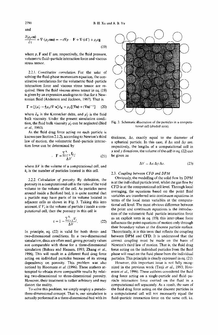
2.2.2. Calculation o f porosity. By definition, the porosity in a computational cell is the ratio of the void volume to the volume of the cell. As particles move around inside a fluidized bed, it is quite normal that a particle may have parts of its volume located in adjacent cells as shown in Fig. 3. Taking this into account, if Vi is the volume of particle i inside a computational cell, then the porosity in this cell is

e = 1 - - - 2 ~ l V i (22) AV

In principle, eq. (22) is valid for both three- and two-dimensional conditions. In a two-dimensional simulation, discs are often used, giving porosity values not comparable with those for a three-dimensional simulation (Bideau and Hansen, 1993; Zhang et al., 1996). This will result in a different fluid drag force acting on individual particles because of its strong dependency on porosity. This problem was also noticed by Hoomans et al. (1996). These authors attempted to obtain more comparable results by relat- ing two-dimensional to three-dimensional porosity. However, their treatment is rather arbitrary and may distort the reality.

To solve this problem, we simply employ a pseudo- three-dimensional concept. That is, our simulation is actually performed in a three-dimensional bed with its

Fig. 3. Schematic illustration of the particles in a computational cell (shaded area).

thickness, Az, exactly equal to the diameter of a spherical particle. In this case, if Ax and Ay are, respectively, the lengths of a computational cell in x and y directions, the volume of the cell in eq. (22) can be given as

AV = Ax Ay Az. (23)

2.3. Couplin9 between CFD and D P M Obviously, the modelling of the solid flow by DPM

is at the individual particle level, whilst the gas flow by CFD is at the computational cell level. Through local averaging, the equations based on the point fluid variables are transferred into continuum equations in terms of the local mean variables at the computational cell level. The most obvious difference between the point and continuum equations is the introduction of the volumetric fluid-particle interaction force as an explicit term in eq. (19); this inter-phase force influences the point equations of motion only through their boundary values at the discrete particle surface. Theoretically, it is this term that reflects the coupling between DPM and CFD. It is understood that the correct coupling must be made on the basis of Newton's third law of motion. That is, the fluid drag force acting on the individual particles from the fluid phase will react on the fluid phase from the individual particles. This principle is clearly expressed in eq. (21).

However, this important issue is not fully recognized in the previous work (Tsuji et aL, 1993; Hoo- mans et al., 1996). These authors considered the fluid drag force acting on a single-particle and fluid particle interaction force exerted on the fluid in a computational cell separately. As a result, the sum of the fluid drag force acting on the discrete particles in a computational cell will not necessarily equal the fluid-particle interaction force on the same cell, i.e.

Gas-solid flow

Newton's third law of motion is not satisfied. Theoret- ically their model is not correct.

In this work, the combination of DPM and CFD is numerically achieved as follows. At each time step, DPM will give information, such as the positions and velocities of individual particles, for the evaluation of porosity and volumetric fluid-particle interaction force in a computational cell by eq. (21). CFD will then use these data to determine the gas flow field which, by eq. (8), yields the fluid drag forces acting on individual particles. Incorporation of the resulting forces into DPM will produce information about the motion of individual particles for the next time step. This procedure clearly indicates that the description of the continuum gas and discrete particle flows in a fluidized bed should be obtained only when DPM and CFD are properly combined - - a fact that ex- plains why the present model is referred to as a DPM-CFD model.

2.4. Solut ion technique

The selection of appropriate numerical schemes for solving the DPM and CFD equations is very important as it not only affects the solution accuracy but also the efficient use of the computer resources. Since the governing equations in the DPM and CFD are different, different solution schemes have to be used.

The explicit time integration method is widely used to solve the translational and rotational motions of a system of discrete particles in the DPM simulations (e.g. see Cundall and Strack, 1979; Tsuji et al., 1993; Hoomans et al., 1996). The straightforward formula- tion without an excess requirement for computer memory is the main advantage of this method. How- ever, due to the constraint for numerical stability, the time step used for such a simulation should be very small. This is because particles do not detect the contact with others until they finish the movement in one time step. The displacements may be overesti- mated, which introduces fictitious elastic energy for particle collisions and hence leads to unrealistic re- suits. To avoid this problem, the so-called predictor- corrector method [Hughes, 1982) has been incorporated into the present simulation.

The equations involved in the predictor-corrector procedure are given below for solving eq. (1) and the similar equations can be developed for solving eq. (2).

For the predictor stage,

v~ = vi + At(1 - ~)ai (24)

r~ ---- r i + Arv i + 0.SAz2(1 - 2fl)ai (25)

and the force balance after predictor stage,

k,

mia~'=fs . i+ Z fPi i+fP. iJ)+mig • (26) j - 1

For the corrector stage,

v c = v~' + Ar ~a~' (27)

r~ = r~' + Az 2 fla~ (28)


where ai and ri are the acceleration and position vector of particle i, respectively, the superscripts, p and c, represent the values estimated at the predictor and corrector stages, ~t and fl are the Newmark parameters which control the accuracy and stability of the method (Newmark, 1959). For this work,

= 0.5 and fl = 0.25 are chosen to achieve consistency with a constant variation of velocity in a given time interval.

The conventional SIMPLE method (Patankar, 1980) is used to solve the equations for the fluid phase. The governing equations are discretized in finite volume form on a uniform, staggered grid. The second-order central difference scheme is used for the pressure gradient and divergence terms. The first- order up-wind scheme is used for the convection term and a second-order Crank-Nicolson scheme is used for the time derivative.

3. SIMULATION CONDITIONS

3.1. Boundary condit ions

The simulation conditions are similar to those of Tsuji et al. (1993) and Hoomans et al. (1996). The simulated fluidized bed consists of a rectangular container of dimension 0.9 × 0.15 × 0.004 m with a jet slot of 0.01 m in width at the centre of the bottom wall. The calculation domain along with the grid arrangements are shown in Fig. 4. The left, bottom and right walls as well as the top exit consist of the whole calculation domain boundaries. To study effectively the start-up stage of fluidization process, the height of the bed used in the present simulation is 0.9 m, much higher than those used in the previous simulations.

In the CFD simulation, as the finite-volume method is used, no nodes lie on the boundaries. The boundary values for fluid variables are set by inclu- ding an extra point outside of the boundary with a prescribed value. The value at the boundary is then obtained by averaging that point and the nearest point in the calculation domain. For the fluid velocity, the no-slip boundary condition applies to left, bottom and right walls and zero normal gradient condition to the top exit. At the central jet, a plug profile for fluid velocity is specified at a given value. For the porosity and pressure correction, the zero normal gradient condition applies along the boundaries. The pressure, which is obtained from the pressure correction at all interior points, is obtained on the boundaries by using a second-order extrapolation from the interior points.

In the DPM simulation, the inter-particle force models discussed in Section 2.1.1 are also applied to the collision between a particle and wall, with the corresponding wall properties used in the simulation. However, the wall is assumed to be so rigid that no displacement and movement result from this collision.

3.2. Select ion o f parameters

To solve the DPM and CFD equations, parameters involved must be specified a priori. Table 1 lists the parameters used in this simulation. Of particular im- portance is the determination of the computational


bed width=O. 15 m P, .

I

I

I i

i

!

!

I I i ! I I

r i

gas jet

Fig. 4. Calculation domain and grid arrangement for the present simulation.

time step and viscous contact damping coefficient, which are often determined with a large degree of empiricism in the literature. As discussed below, the present simulation uses a rather simple but effective method to determine these parameters.

3.2.1. Time step. As the magnitude of the length scale of D P M is much smaller than that of CFD, the time step used in the numerical simulation should be determined from the D P M constraints. Obviously, under the condition of conserving the energy during an elastic collision, the larger this time step, the more efficient use of the computer resource. This time step is here determined by simulating the dropping of a particle from a fixed height to a flat wall of the same properties. It is evident that the energy conservation is met if a particle can bounce back to its initial dropping height. The maximum time step giving such results can be found after a series of tests using different time steps; here a value of 1.5 × 10 -5 s is chosen under the present simulation conditions (see Table 1).

Although the above time step is determined from the situation of the collision between a particle and a fiat wall, it is also applicable to the collision between particles because the underlying mechanisms are essentially the same.

3.2.2. Viscous contact damping coefficient. The viscous contact damping coefficient is determined based on the mechanisms involved in an inelastic collision process. The magnitude of this damping should consume the energy at a realistic rate. As the collisions involved are actually a multi-collision dynamic process, it is extremely difficult to determine this coefficient theoretically. In this work, this parameter is determined from a number of numerical tests involving the collision of a particle with a flat wall, as described below.

Using the time step determined in Section 3.2.1, different viscous contact damping coefficients are tested. It is known that the right viscous contact damping coefficient should correctly reflect the energy loss after a collision, which can be measured by the

Table 1. Parameters used for the present simulation*

Solid phase Gas phase

Particle shape Spherical Viscosity,/~f Number of particles 2400 Density, p: Particle diameter, D 0.004 m Bed width Particle density, pp 2700 kg m- 3 Bed height Spring constant, ~¢, or ~:t 50,000 N m- 1 Bed thickness Friction coefficient, 7 0.3 Orifice width Viscous contact damping Cell width, Ax coefficient, q, or qt 0.15 Cell height, Ay

1.8x 10--s kgm- 1 s - l 1.205 kg m - 3 0.15m 0.9 m 0.004 m 10mm 10 mm 20 mm

* The wall properties such as to, ), and r/are the same as those for particles.

Gas solid flow in

coefficient of restitution, e, defined as

Vl e = - - (29a)

VO

or in terms of height

e = (29b)

where vo, ho, and vl, hi are, respectively, the velocities and the maximum heights of the particle before and after the collision. For the ideal case without energy loss (e = 1), the viscous damping coefficient should be equal to zero. In the present simulation, a realistic value of 0.9 is chosen for the coefficient of restitution. Corresponding to this value, the viscous damping coefficient is determined to be 0.15.

3.3. Initial conditions Initially, the fluid is at rest anywhere in the calcu-

lation domain with 2400 particles (D = 4 × 10 -3 m) inside. The initial particle configuration in the calculation domain is generated as follows. The container is divided into a set of small square cells with its length equal to the diameter of particles. Along the height of the container, each adjacent cell offsets a distance equal to the particle radius. Then 2400 particles are randomly positioned in these cells and allowed to fall down under gravity. The motion of particles is determined by the above developed model which has also taken into account the air flow as a result of particle dropping. A stable packing configuration is finally generated after sufficient time of simulation.

a fluidized bed 2793

A number of initial particle configurations have been generated in this way, giving slightly different packing structures. One of these packing processes is shown in Fig. 5; its final stage (t = 0.8 s) is used as the initial input data for the fluidization simulation. Regular packing structure is observed in some regions, which is mainly due to the wall effect (Jullien et al., 1993; Zhang et al., 1996). However, the packing structure as a whole is reasonably comparable with those measured (Bideau and Hansen, 1993).

Note that the initial input data for fluidization simulation should include not only the particle coordinates but also forces and torques which come with the positioning of particles in a packing process. Use of the particle coordinates alone will give different fluidization flow patterns, particularly at the initial stage. This suggests that the packing structures, constructed by other simulation techniques without considering the forces and torques, may not be so appropriate for realistic simulations.

4. RESULTS AND DISCUSSION

4.1. Relationship between bed pressure drop and superficial gas velocity

To test the validity of the proposed model, an attempt has been made to establish the relationship between the bed pressure drop and superficial gas velocity, Totally, 23 runs of simulation are carried out, corresponding to the cases with an increasing or decreasing superficial gas velocity. The cases corresponding to the increasing superficial gas velocity are simulated under the same boundary and initial conditions outlined in Section 3 with different gas jet

~ Time=0.00 (sec) 0.6 Tirne=0.20 (sec) 0.6 Time=0.80 (sec)

0,~ 0.4

0.,~ 0.2

0.(] 0.0

Fig. 5. Particle configurations at different times in a simulated packing process.

2794

velocities. The cases corresponding to the decreasing superficial gas velocity are simulated by successively decreasing the superficial gas velocity, with the final results at a higher velocity as the initial input data for the simulation at next (lower) velocity. All the simulations are carried out at a HP-735 workstation and about 9 h of CPU time are required to run for 1 s real time.

The superficial gas velocity, here as an alternative to the gas jet velocity, is defined as the total volumetric gas flow rate divided by the entire bed cross-sec- tional area. The bed pressure drop, Ap, is the gas pressure difference between the bottom and top along the symmetric line of the bed. Because bed pressure drop fluctuates with time, a representative mean value, A/~, over a period of time is required. A/~ is here evaluated by the following equation:

A/5 - ~ A p d r (30) T 2 - - 171

where zl and z2 are, respectively, the initial and final times for the calculation of mean pressure drop. Note that zl should be large enough to eliminate the effect of the start-up, and z2 can be the end time of a simulation.

Figure 6 shows the results, where four stages can be identified, i.e. a fixed bed stage (point A to B), fully fluidized bed stage (point C to D), incipient fluidization stage (point C to E) and defluidization stage (point E to F). The results are qualitatively in good agreement with those established in the literature (Davidson et al., 1985; Ishikura et al., 1986).

The fixed-bed stage actually relates to the gas flow in a packed bed. No obvious movement of particles is


observed at this stage. The bed pressure drop in- creases with increasing the superficial gas velocity until a critical point, G, is reached. After this point the bed pressure drop starts to decrease with increasing the superficial gas velocity. The small difference between the bed pressure drops at points G and B corresponds to the slight rearrangement of particles, resulting in an improved bed porosity.

The sharp decrease of bed pressure drop from point B to C reflects a significant change in particle configuration as a result of fluidization. As will be discussed in the following section, at the fully fluidized-bed stage, bubbles and slugs are generated continuously during the gas flow and particles move vigorously inside the bed. This stage is characterized by an al- most constant bed pressure drop. Starting from point C, it can extend up to the terminal velocity, although this is not attempted in the present study (note that a higher bed is required to accommodate particles at the start-up stage at a higher superficial gas velocity).

On the other hand, decreasing the superficial gas velocity from point C to E will yield an incipient fluidization stage. This will allow the minimum fluidization velocity (point E) to be determined, where a value of 1.8 m s- ~ is found. Interestingly, this value is very close to the value of 1.77 m s- ~ estimated from the well-known Wen and Yu correlation (1966). From point C to E, the bed pressure drop is essentially maintained at the same level as that of the fully fluidized-bed stage. The slugs and bubbles are still observed at this stage; however, its intensity is at- tenuated gradually from point C to E. The solid flow patterns at point E are shown in Fig. 7, indicating that at the minimum fluidization velocity, a gas bubble forms only at the jet region and the gas can readily

Q .

" o

3.0x10 4

7.0xl 0 3

2.0x10 3

6.0x10 2

0.0

. . . . I . . . . I ' ' ' ' I ' ' ' ' [ . . . . I . . . . I

- e Increasing vel°city I - - I I Decreasing velocity~ ~ 1 ~

, J , = I ~ , , , E ~ , , , I , , , ~ I , , , J I , h , , J . . . .

0.5 1.0 1.5 2.0 2.5 3.0

Superficial gas velocity (m/s)

Fig. 6. Bed pressure drop vs superficial gas velocity.

3.5

Gas-solid flow in a fluidized bed 2795

O.E Time=0.12 (sec I 0.6

O.Z 0.4

Time=0.22 (sec I Time=0.32 (sec) 0.6

0.4

Time=0.42 Isec~

v , v

Fig. 7. Particle configurations at point E (see Fig. 6) when superficial gas velocity is equal to minimum fluidization velocity.

2 . 0 x 1 0 4 ' ' i ' ' ' I I ' ' ' E I ' '

1.5X10 4

0 -

t - t

o 1"0x104

e n

5.0x10 a

O.OxlO ° 0 2 4 6 8 10

Time (sec)

Fig. 8. Bed pressure drop vs time when superficial gas velocity is equal to 2.8 m s- 1.

12

flow through the bed without resulting in a rigorous solid flow.

Further decreasing the superficial gas velocity from point E will give a defluidization stage, where no bubbles are generated. The bed pressure drop continuously decreases with decreasing superficial gas velocity. However, the curve does not coincide with

that at the fixed bed stage, because of different particle configurations.

The distinct hysteretic feature of the bed pressure drop vs superficial gas velocity is the most important fluidization characteristic for a powder. To date, this feature cannot be predicted by any models in the literature. The successful prediction of this feature


provides an important example to validate the proposed model.

4.2. Simulated fluidization behaviour The simulated fluidization behaviour will be dis-

cussed for a typical case at the fully fluidized bed stage when the gas jet velocity equals 42 m s ] (superficial gas velocity equals 2.8 m s- 1). Figure 8 shows a plot of bed pressure drop against time for this case. Two

regions are identified here: the start-up (z < 1 s) and stable fluidization stages. The maximum bed pressure drop at the start-up stage is much higher than that at the stable stage because of the need to overcome the inter-particle locking. After the start-up stage, the bed pressure drop fluctuates with time around a mean value given by eq. (30).

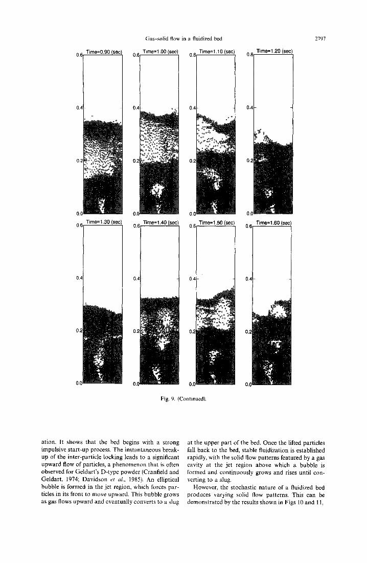
Figure 9 shows the simulated solid flow patterns at the early stage from the start-up to the stable fluidiz-

Time=0.10 ( s e c ) Time=0.20 (sec~ 0.6

0.4

0.2

0.0 Tirne=0.50 (see~ 0.6f Time=0.60 (sec)

o ° ° o o

0.4 ~

g

0.2 °

0.0

TirnP.=0.7f) (sec~

TimA=fl.40 (~t~3

Fig. 9. Particle configurations from the start-up stage to stable fluidization when superficial gas velocity is equal to 2.8 m s- 1.

0.6

0.E

Time=0.90 Isec~

Tirne=1.30 (sec~

Gas solid flow in a fluidized bed

0.6 Time=1,00 ( s e c ) Timo.=1.1i3 (go.e~

0.4

0.2

O.C

o~

~o ~%°°o:~.~

0.6

v . v

Time= 1.50 (sec)

Fig. 9. (Continued).

Time=l ~O ~.~An]

0.6 Time=1.60 (sec)

2797

ation. It shows that the bed begins with a strong impulsive start-up process. The instantaneous break- up of the inter-particle locking leads to a significant upward flow of particles, a phenomenon that is often observed for Geldart's D-type powder (Cranfield and Geldart, 1974; Davidson et al., 1985). An elliptical bubble is formed in the jet region, which forces particles in its front to move upward. This bubble grows as gas flows upward and eventually converts to a slug

at the upper part of the bed. Once the lifted particles fall back to the bed, stable fluidization is established rapidly, with the solid flow patterns featured by a gas cavity at the jet region above which a bubble is formed and continuously grows and rises until con- verting to a slug.

However, the stochastic nature of a fluidized bed produces varying solid flow patterns. This can be demonstrated by the results shown in Figs 10 and 11,

2798 B.H. Xu and A. B. Yu

0.6 Time=1.74 (sec) Tim~=l 7R/~An~ 0.6 Time=1.82 (sec

0.4 0,4

0.2 0.2

0.0 0.0

0.6

0.4

0.2

0.0

Time=1.90 (sec) Time=1.94 (sec) Time=l ~8 (s~'~.~ Time=2.02 (sec 0.6 0.E

0.4 0.4

0.2 0.2

0.0 0.0

Fig. 10. A typical example showing the 's-shape' flow path of a gas bubble when superficial gas velocity is equal to 2.8 m s - 1.

Gas-sol id flow in a fluidized bed 2799

0,6

0.6

Time=2.60 (sec) Timp.=2.AA (.qAc~

Time=2.84 (see

o.6[

I

I I

Time=2.78 (sec)

Tim~.=~ .qfl I.~'~.~ Tim~.='2 ~A/~p.n~ TimA=.q N 9 / ~

(a)

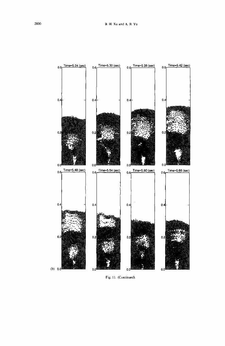
Fig, 11. Results showing different particle configurations in forming a slug when superficial gas velocity is equal to 2.8 m s - ~ at different times: (a) z = 2.6 to 3.02 s; (b) z = 5.24 to 5.66 s.


Time=5.24 (sec) 0.6 Time.=R .q13/.~Anl TImA=R ~ I.q,s~.l TimA=R 49 I~Anl

0.4

0.2

0.0

0.E Time=5.48 (sec)

0.4

0.2

(b) 0.0

Time.=.~.~0 (s~e3


0.6 Time=5.66 (sec

0.4

0.2

0.0

0.4

0.3

0.2

0.1

0.0 0.00 0.05 0.10 0.15


which correspond to different simulation times. In particular, Fig. 10 suggests that a bubble may flow following a 's-shape' path, and Fig. 11 indicates that slugging patterns can differ significantly.

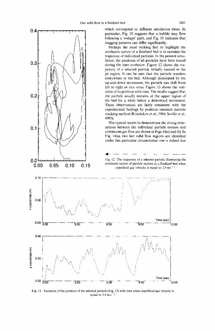
Perhaps the most striking fact to highlight the stochastic nature of a fluidized bed is to examine the trajectory of individual particles. In the present simulation, the positions of all particles have been traced during the time evolution. Figure 12 shows the trajectory of a selected particle initially located in the jet region. It can be seen that the particle wanders everywhere in the bed. Although dominated by the up-and-down movement, the particle can shift from left to right or vice versa. Figure 13 shows the variation of its position with time. The results suggest that the particle usually remains at the upper region of the bed for a while before a downward movement. These observations are fairly consistent with the experimental findings by positron emission particle tracking method (Kondukov et al., 1964; Seville et al.,

1995). The typical results to demonstrate the strong inter-

actions between the individual particle motion and continuum gas flow are shown in Figs 14(a) and (b). In Fig. 14(a), two fast solid flow regions are identified under this particular circumstance: one is indeed due

Fig. 12. The trajectory of a selected particle illustrating the stochastic nature of particle motion in a fluidized bed when

superficial gas velocity is equal to 2.8 m s- ~.

0.15 [

/ /

) 0.08 ""/ "/''

, J / /

j

i / , / I '/

I v

T ime (sec) 0 .00 0 .00 '3.00 '6.00' '9.00' ' ' 12.00

0.40

v

£ O

0.20

/ @

\ A I \ ,' " ," / I' '~, t

"\. ",\ J i \, i' / ' , \ i I

x, i \ ' \ \ i ~

T ime (see) 0 .00 0.~00 '3.00 ' '6.00 . . . . . 9 .00 . . . . 12.00

Fig. 13. Variation of the position of the selected particle (Fig. 12) with time when superficial gas velocity is equal to 2.Sins 1.


(a)

0.6 Time=7.32 (sec,

0.,4

0,. ~

0.C

Time=7 40 (.~e~.l

(b)

Time=7.32 (sec I O . ~ ' p . , t t l t t l l f T t ~

, , * t t t t ~ t T l l t t ~ p , , t ~ ? l t l l l ~ t t q ~ , , I I I I T I T ~ ? r ? ~ , , , t t t l l l ? l l ~ r , , , , , I I I I I T [ I I I , , , , t I t ? t IT [?TT~ , , , ~ r l l ? t f T t t l , , , , ~ ? I I ~ f T T I ] , , , , ~ ? I r ? t f l ? t f ,

0.~ [ ~ , , t t f / l ? t l t | ~ t t , t t I I t l t t l ~ l t

0.2

O . C l i m ~ ~ d

Time=7.40 (sec)

. . . . . , ~ l l l l l l . . . . . i t l ~ l l l . . . . . t l l l l l l

. . . . . . . . t T I l l l 0.4 , , l i l t I-

. . . . . . . . ~Itr

Tim~---7.44/~ecl

Fig. 14. Typical results when superficial gas velocity is equal to 2.8 m s - 1 demonstrating the distributions of (a) velocity of solid particles; (b) velocity of gas phase; (c) total forces (N); and (d) torques acting on

individual particles (N m).


0.6 Time=7.32 (s~ql

6E-1 5E-1 4E-1

2E-1 1E-1

Tim~==7 4.4 I¢~r%

(c)

0.6

0.4

05

0.( (d)

Time=7.32 (sec

3E-4 2E-4 2E-4 1E4 6E-5

0.E

v . v


Time=7.40 (sec~

7E-1 5E-1 4E-1 3E-1 1E-1


0

C L

0

E E

2.0

1.0

0.0 0

' I '

h i I I

2

r ' ' ' ' J ' ' ' ' I . . . . t

4 6 8 10 12 Time (sec)

Fig. 15. Maximum overlap ratio vs time when superficial gas velocity is equal to 2.8 m s-1.

to the gas dragging in the main stream [see Fig. 14(b)] and the other is due to the falling of the particles to fill in the vacant space. There is a big vortex developed corresponding to these two fast flow regions, which promotes solid mixing considerably. From Fig. 14(b), it can also be seen that the gas flows toward the regions of high porosity. This high preferential flow will lead to a strong non-uniform fluid drag force distribution inside the bed, which in turn will greatly affect the solid flow patterns.

As indicated in eq. (1), the motion of a particle is governed by the gravitational, fluid drag and inter- particle forces. These forces, except for the gravity, vary with time and position. Figures 14(c) and (d) show the results to highlight this point. It appears that the resultant force and torque acting on the individual particles are quite localized. In particular, the large forces usually occur in pairs, suggesting that the inter-particle force is more important than the fluid drag force in terms of their maxima. Examining the results with reference to the flow patterns shown in Figs 14(a) and (b), suggests that the fast flow of gas and particles in the jet region does not necessarily correspond to large forces acting on the individual particles. Information about the transient forces at the individual particle level is important to understanding the complicated fluidization phenomena such as particle attrition or breakage. Therefore, the proposed model provides an effective technique to enhance these studies.

The deformation of the particles during a collision can be measured by the ratio of the distance between the mass centres of two colliding particles to the sum of their radii. One minus this ratio is here defined as the overlap ratio. The maximum overlap ratio among

all the particles considered varies with time as shown in Fig. 15. There is also a strong peak corresponding to the start-up stage as identified from the bed pressure drop curve (Fig. 8). The maximum overlap ratio fluctuates with time. Except for a maximum value of 1.7% at the start-up stage, its value in the present simulation is well below 1%, indicating the effec- tiveness of the present approach. Small overlaps among particles are essential in order to obtain a realistic simulation of a fluidization process.

Figure 16 shows the solid flow patterns for the ideal case (q = 0 and 1' = 0), which differ from those for the corresponding non-ideal, realistic case (Fig. 9). It can be observed that after the start-up stage, a bubble is continuously generated at the jet region and then grows to convert to a slug, and particles scatter over the upper part of the bed. Interestingly, different from the non-ideal case as shown in Fig. 9, a bubble experi- ences its generation, growth and burst-out procedures before a new bubble is formed, and this cycle is quite stable as shown in Fig. 17. This difference indicates that material properties, as reflected by simulation parameters, affect fluidization behaviour. Therefore, realistic parameters should be chosen in order to obtain realistic simulated results.

5. CONCLUSIONS

A comprehensive understanding of the complex phenomena in a fluidized bed necessitates that this gas-solid two-phase flow system should be studied and modelled not only at the processing equipment and/or computational cell level but also at the individual particle level. For this purpose, a combined DPM-CFD model has been developed to simulate the

Gas solid flow in a fluidized bed 2805

0,( Time=O. 10 (sec I Time=0.30 (sec~ Time=0.40 (sec~

Time=f}.fiO (~en~ Tim~=O.RO I~t=~.'~ Time=0.70 ( ~ e c ~ Tim~=O.80 (~.n~

Fig. 16. Particle configurations from the start-up stage to stable fluidization when superficial gas velocity is equal to 2.8 m s-1 under ideal conditions (~/= 0 and 7 = 0).

2806 B . H . X u a n d A. B. Yu

0.6 Izime 0.90,sec, I ' o ° oo o

Ooo~°: ° ~O°o 0.4 -0 ooo , o

0.2

0.0

0.6 Time=l'30 (sec) Time=1.50 (aec~

TimP~=l 2N (AAP3

TimA:I tqi3 [~Ac.~

Fig. 16. (Cont inued) .

Gas solid flow in a fluidized bed 2807

2.0X10 4

1.0xl 0 4

8

m 5.0X10 3 I

O.OxlO ° 0 1 2 3 4

Time (sec)

Fig. 17. Bed pressure drop vs time when superficial gas velocity is equal to 2.8 m s i under ideal conditions (r/= 0 and 7 = 0).

gas-solid flow in a fluidized bed, in which the motion F of individual particles is obtained by solving Newton's second law of motion and the gas flow by the g Navier-Stokes equation based on the concept of local ho average. The coupling between the continuous gas flow and the discrete particle motion at different hi length and time scales is achieved directly by applying the principle of Newton's third law of motion to both I phases. The results presented in this work clearly kc indicate that this model can provide detailed realistic dynamic information in a fluidized bed at different ki levels from the processing equipment to the individual particle. This combined D P M - C F D approach will be very useful in elucidating the mechanisms governing the fluid-solid two-phase flow and studying the complex phenomena in such a flow system in a cost- effective way.

Acknowledgement The authors are grateful to the Department of Education,

Employment and Training (DEET) for financial support through the Overseas Postgraduate Research Scholarship (OPRS) scheme (to B. H. Xu), and Dr P. Zulli, Dr J. Truelove and Dr A. Brent of BHP Research for their interest and helpful discussion.

a

Cdo

D e

f ~o

N O T A T I O N

particle acceleration, m s-2 fluid drag coefficient on an isolated particle, dimensionless particle diameter, m coefficient of restitution, dimensionless force, N fluid drag force on an isolated particle. N

m

n

P Ap

r

R Re t

T II

¥

V

DO

Vl

AV X

Ax

Y Ay Az

volumetric fluid-particle interaction force, Nm-:~ gravitational acceleration, m s-2 maximum height of a particle before collision, m maximum height of a particle after collision, m moment of inertia of particle, kg m 2 number of particles in a computational cell, dimensionless number of particles in contact with particle i, dimensionless particle mass, kg unit vector along the normal direction pressure, Pa bed pressure drop, Pa mean bed pressure drop, Pa particle position vector, m particle radius, m Reynolds number, dimensionless unit vector along the tangential direction torque, N m fluid velocity, m s 1 particle velocity, m s- volume, m 3 particle velocity before collision, m s- 1 particle velocity after collision, m s- 1 volume of a computational cell, m 3 x coordinate of particle, m computational cell length in x direction, m y coordinate of particle, m computational cell length in y direction, m thickness of a pseudo-three-dimensional bed, m

2808

Greek letters Newmark parameter, dimensionless

fl Newmark parameter, dimensionless 6 displacement or overlap between two con-

tacting particles, m 6k Kronecker delta, dimensionless A~ incremental displacement, defined by eqs

(14)-(17), m porosity, dimensionless coefficient of friction, dimensionless

F fluid viscous stress tensor, kg m - i s -2 particle spring constant, N m 1

/~ shear viscosity, kg m- ~ s - /t' bulk viscosity, kg m- 1 s- ~/ coefficient of viscous contact damping,

kgs -1 p density, kg m- 3

time, s z~ initial time for calculation of mean pressure

drop, s 32 final time for calculation of mean pressure

drop, s A~ time step, s Az' actual collision time, s Z empirical coefficient defined by eq. (10), di-

mensionless co particle angular velocity, s

Subscripts c contact d damping f fluid phase i particle i ij between particle i and j j particle j ji between particle j and i n normal component p particle phase r relative t tangential component x x component y y component

Superscripts c corrector stage p predictor stage

REFERENCES

Anderson, T. B. and Jackson, R. (1967) A fluid mech- anical description of fluidized beds. I&EC Fundam. 6, 527-539.

Bi, H. T. and Grace, J. R. (1995) Flow regime diagra- ms for gas-solid fluidization and upward transport. Int. J. Multiphase Flow 21, 1229-1236.

Bideau, D. and Hansen, A. (eds) (1993) Disorder and Granular Media. Elsevier Science Publishers B. V., Amsterdam, The Netherlands.

Bird, R. B., Stewart, W. E. and Lightfood, E. N. (1960) Transport Phenomena. Wiley, New York.


Cranfield, R. R. and Geldart, D. (1974) Large particle fluidization. Chem. Engng Sci, 29, 935-947.

Crisfield, M. A. and Shi, J. (1994) A co-rotational element/time-integration strategy for non-linear dynamics. Int. J. Numer. Methods Engn 9 37, 1897- 1913.

Cundall, P. A. and Strack, O. D. L. (1979) A discrete numerical model for granular assemblies. Geotech- nique, 29, 47 65.

Davidson, J. F., Cliff, R. and Harrison, D. (eds), (1985) Fluidization, 2nd Edn. Academic Press, London, UK.

Di Felice, R. (1994) The voidage function for fluid- particle interaction systems. Int. J. Multiphase Flow 20, 153 159.

Drake, T. G. and Walton, O. R. (1995) Comparison of experimental and simulated grain flows. ASME J. Appl. Mech. 62, 131 135.

Ergun, S. (1952) Fluid flow through packed columns. Chem. Engng Prog. 48, 89-94.

Geldart, D. (1973) Types of gas fluidization. Powder Technol. 7, 285-292.

Gidaspow, D. (1994) Multiphase Flow and Fluidiza- tion. Academic Press, San Diego.

Grace, J. R. (1986) Contacting modes and behaviour classification of gas-solid and other two-phase sus- pensions. Can. J. Chem. Engng 64, 353-363.

Haft, P. K. and Anderson, R. S. (1993) Grain scale simulations of loose sedimentary beds: the example of grain-bed impacts in aeolian saltation. Sedimen- tology 40, 175 198.

Hoomans, B. P. B., Kuipers, J. A. M., Briels, W. J. and Van Swaaij, W. P. M. (1996) Discrete particle simulation of bubble and slug formation in a two-dimensional gas-fluidised bed: a hard-sphere approach. Chem. Engng Sci. 51, 99-118.

Hu, H. H. (1996) Direct simulation of flows of solid- liquid mixtures. Int. J. Multiphase Flow 22, 335-352.

Hughes, T. J. R. (1976) Stability, convergence and growth and decay of energy of the average acceleration method in nonlinear structural dynamics. Comput. Struct. 6, 313-324.

Hughes, T. J. R. (1982) Implicit-explicit finite element techniques for symmetric and nonsymmetric systems. In Recent Advances in Non-linear Computa- tional Mechanics, eds E. Hinton, D. R. J. Owen and C. Taylor, Chap. 9, pp. 255-267. Pineridge Press Limited, Swansea, U.K.

Hughes, T. J. R., Caughey, T. K. and Liu, W. K. (1978) Finite-element methods for nonlinear elas- todynamics which conserve energy. ASME J. Appl. Mech. 45, 366-370.

Ishikura, T., Shinohara, H. and Funatsu, K. (1986) Minimum spouting conditions for particle mixtures. In Encyclopedia of Fluid Mechanics, IV, ed. N. P. Cheremisinoff, Chap. 34, pp. 1077-1087. Gulf Publishing Company, Houston, TX, U.S.A.

Jiang, Z. and Haft, P. K. (1993) Multiparticle simulation methods applied to the micromechanics of bed load transport. Water Resour. Res. 29, 399-412.

Johnson, K. L. (1985) Contact Mechanics. Cambridge University Press, Cambridge, U.K.

Jullien, R., Meakin, P. and Pavlovitch, A, (1993) Growth of packings. In Disorder and Granular Me- dia, eds Bideau and Hansen, Chap. 4, pp. 103-131, Elsevier, Science Publishers B. V., Amsterdam, The Netherlands.

Gas-solid flow in a fluidized bed

Kondukov, N. B., Kornilaev, A. N., Skachko, I. M., Akhromenkov, A. A, and Kruglov, A. S. (1964) An investigation of the parameters of moving particles in a fluidized bed by a radioisotopic method. Int. Chem. Engng 4, 43-47.

Langston, P. A., Tiizi.in, U. and Heyes, D. M. (1995) Discrete element simulation of granular flow in 2D and 3D hoppers: dependence of discharge rate and wall stress on particle interactions. Chem. Engng Sci. 50, 967-987.

Langston, P. A., Tiizfin, U. and Heyes, D. M. (1996) Distinct element simulation of interstitial air effects in axially symmetric granular flows in hoppers. Chem. Engng Sci 51, 873-891.

Liang, S.-C., Hong, T. and Fan, L.-S. (1996) Effects of particle arrangements on the drag force of a particle in the intermediate flow regime. Int. J. Multiphase Flow 22, 285-306.

Newmark, N. M. (1959) A method of computation for structural dynamics. J. Engng Mech. Div. Proc. ASCE (EM3) 85, 67-94.

Patankar, S. V. (1980) Numerical Heat Transfer and Fluid Flow. Hemisphere, New York, U.S.A.

Richardson, J. F. and Zaki, W. N. (1954) Sedimenta- tion and fluidization: Part I. Trans. lnstn Chem. Engrs 32, 35-53.

Rowe, P. N. (1987) A convenient empirical equation for estimation of the Richardson-Zaki exponent. Chem. Engng Sci. 42, 2795-2796,

Sadd, M. H., Tai, Q. and Shukla, A. (1993) Contact law effects on wave propagation in particulate materials using distinct element modeling. Int. J. Non-linear Mech. 28, 251-265.

Seville, J. P. K., Simons, S. J. R., Broadbent, C. J., Martin, T. W., Parker, D. J. and Beynon, T. D.

2809

(1995) Particle velocities in gas-fluidised beds. In Fluidization VIII, pp. 319-326. Engineering Foun- dation, New York.

Stewart, I. (1992) Warning-handle with care! Nature, 355, 16-17.

Thornton, C. (ed.) (1993) Powders & Grains 93. A. A. Balkema, Rotterdam.

Thornton, C. and Yin, K. K. (1991) Impact of elastic spheres with and without adhesion. Powder Tech- nol. 65, 153-166.

Tsuji, Y., Kawaguchi, T. and Tanaka, T. (1993) Dis- crete particle simulation of two-dimensional fluidized bed. Powder Technol. 77, 79-87.

Tsuji, Y., Tanaka, T. and Ishida, T. (1992) Lagrangian numerical simulation of plug flow of cohesionless particles in a horizontal pipe. Powder Technol. 71, 239-250.

Walton, O. R. (1993) Numerical simulation of inclined chute flows of monodisperse, inelastic, frictional spheres. Mech. Mater. 16, 239-247.

Warr, S., Jacques, G. T. H. and Huntley, J. M. (1994) Tracking the translational and rotational motion of granular particles: use of high-speed photography and image processing. Powder Technol. 81, 41 56.

Wen, C. Y. and Yu, Y. H. (1966) A generalized method for predicting the minimum fluidization velocity. A.I.Ch.E.J. 12, 610-612.

Xie, Y. M. and Steven, G. P. (1994) Instability, chaos, and growth and decay of energy of time-stepping schemes for non-linear dynamic equations. Com- mun. Numer. Methods Engng 10, 393-401.

Zhang, Z. P., Yu, A. B. and Oakeshott, R. B. S. (1996) Effect of packing method on the randomness of disc packings. J. Phys. A: Math. Gen. 29, 2671-2685.

numerical simulation of the gas-solid flow in a fluidized bed by discrete particle method with cfd

Documents

gas flow

continuum gas

bed of particles

gassolid flow features

gas fluidization process

introduction gas fluidization

gasphase equations

motion of individual