Fourth International Symposium on Marine Propulsors smp’15, Austin, Texas, USA, June 2015

Numerical Simulation of Ship Hull Pressure Fluctuation Induced by Cavitation on Propeller with Capturing the Tip Vortex

Keita Fujiyama1

1 Software Engineering Department,

Software Cradle Co., Ltd., Osaka, JAPAN

ABSTRACT

For the designing of ship and propeller, the interaction of

them caused by cavitation is a very important factor and the

preliminary study is needed to explain phenomena for the

development. However, the experiment in the laboratory is

expensive and requires substantial time, which sometimes

makes the experiment difficult. Therefore, Computational

fluid dynamics (CFD) is expected to be an effective tool to

solve the problem in this field. This paper presents the

calculations of ship hull pressure fluctuation induced by

cavitation and the comparison of obtained calculation

results with the experimental data of the previous study. It

also explains the relationship between the pressure

fluctuation components and the cavitation phenomena.

Finally, we evaluated the accuracy and the potential of CFD

for the ship and propeller designing.

Keywords

Numerical Simulation, Cavitation, Pressure Fluctuation,

Tip Vortex

1 INTRODUCTION

The construction of ships has encountered some

environmental problems such as the greenhouse gas

emissions and the noise on marine life, and sought the

solutions including higher fuel efficiency of ships. To build

a "high-performance ship", developers must prepare many

development plans in the design phase, then, review and

choose the best one from them. However, conducting

experiments for all the plans costs huge and takes an

immense amount of time. For this reason, experiments are

done basically only for the final design. Therefore, the

importance of numerical simulations as helpful tools for the

designing process of ships is growing to overcome the

experimental difficulties.

The interaction between the wake of a ship and the rotation

of its propeller causes unsteady cavitation. The cavitation

causes the pressure fluctuation on a ship, which affects both

comfort on board and the fatigue strength of the ship

structure. In addition, there is a possibility that the noise

caused by the cavitation attacks the sea animals. To protect

them, the noise must be controlled and the regulation is now

being prepared. For these reasons, predicting unsteady

cavitation and pressure fluctuation on a ship hull in the

design phase is essential for developing ships.

The studies of the propeller cavitation in the wake of a ship

and the pressure fluctuation on a ship hull, using the

numerical simulations, have been presented by Kanemaru et

al. (2013) and Berger et al. (2013). Kanemaru et al. used the

extended panel method while Berger et al. used the finite

element method around the ship hull and the boundary

element method for the propeller in combination. Moreover,

Hasuike et al. (2011) and Sato et al. (2009) simulated

unsteady propeller-cavitation using CFD based on the finite

element method or the finite volume method. They applied

a non-uniform inflow condition with the distribution of the

wake to the calculation. On the other hand, Kawamura et al.

(2010) and Paik et al. (2013) simultaneously analyzed both

the ship hull and the propeller to calculate the cavitation. In

all these studies, the results show that the first component of

the blade passing frequency of the pressure fluctuation can

be predicted with a certain level of accuracy. However, the

amplitude of higher-level components of the frequency is

not predicted well. Konno et al. (2002) suggested that the

higher-level components of the frequency of the pressure

fluctuation are affected by collapse of the tip vortex

cavitation; however, there were less consideration for the tip

vortex cavitation in the aforementioned calculations.

In this paper, we used a model of a ship and its propeller in

combination to perform numerical simulations of unsteady

cavitation including the tip vortex cavitation. Then, we

compared the numerical results with the experimental

results presented by Kurobe et al. (1983) to examine the

relationships between the cavitation phenomena and the

pressure fluctuation on a ship hull. Lastly, we evaluated the

accuracy and the potential of CFD software as a cavitation

prediction tool used in design and development of ship hulls

and propellers.

2 NUMERICAL METHOD

All simulations in this paper were performed by the

SC/Tetra Version 11, which is the commercial navier-stokes

solver based on a finite volume method. In these

calculations, the combination of the compressibility two

phase one fluid model by Okuda et al. (1996) and the full

cavitation model by Singhal et al. (2002) was used as the

cavitation calculation method, and the SST-SAS model was

used as the turbulence model which is the effective method

for the transient cavitation analysis reported by our previous

paper (2012).

2.1 Cavitation Model

In this paper, relative motions between vapour and liquid

are neglected since the flows are assumed to be uniform. In

addition, a barotropic relation is used and the governing

equations of mass and momentum are formally the same as

those of the single phase flows.

Mixture density is described as follows:

𝜌 = ∑ 𝛼𝑁𝜌𝑁 (1)

where, N denotes phase and 𝛼 volume fraction. By using

this mixture density, mass and momentum conservation

equations are described as follows:

𝜕𝜌

𝜕𝑡+

𝜕𝜌𝑢𝑖

𝜕𝑥𝑖

= 0 (2)

𝜕𝜌𝑢𝑖

𝜕𝑡+

𝜕𝜌𝑢𝑖𝑢𝑗

𝜕𝑥𝑗

= −𝜕𝑃

𝜕𝑥𝑖

+𝜕𝜏

𝜕𝑥𝑗

(3)

where, 𝜏 indicates shear stress.

Cavitating flows are applied as compressible flows. Thus

the barotropic relation is employed to the equation of the

state. Mixture density containing a non-condensable gas can

be specified by mass fraction instead of volume fraction.

1

𝜌=

𝑌𝑣

𝜌𝑣

+𝑌𝑔

𝜌𝑔

+1 − 𝑌𝑣 − 𝑌𝑔

𝜌𝑙

(4)

where, 𝑌𝑣 and 𝑌𝑔 denote mass fraction of vapour and a non-

condensable gas, respectively. Mass fraction of a non-

condensable gas is assumed to be constant analysis

parameter. Density of the non-condensable gas is obtained

by the following equation.

𝜌𝑔 =

𝑃

𝑅𝑇 (5)

where, R is a gas constant of the non-condensable gas and

the flow field is assumed to be isothermal because

temperature T is also a constant.

Mass fraction of vapour is calculated by the transport

equation below.

𝜕𝜌𝑌𝑣

𝜕𝑡+

𝜕𝜌𝑢𝑖𝑌𝑣

𝜕𝑥𝑖

= 𝑅𝑒 − 𝑅𝑐 (6)

The right-hand side is source terms indicating evaporation

and condensation which are modelled by the full-cavitation

model by Singhal et al (2002).

𝑅𝑒 = 𝐶𝑒

√𝑘

𝜎𝜌𝑙𝜌𝑣√

2

3

𝑃𝑣 − 𝑃

𝜌𝑙

(1 − 𝑌𝑣 − 𝑌𝑔) (7)

𝑅𝑐 = 𝐶𝑐

√𝑘

𝜎𝜌𝑙𝜌𝑙√

2

3

𝑃 − 𝑃𝑣

𝜌𝑙

𝑌𝑣 (8)

where, k denotes turbulent kinetic energy, 𝜌𝑙 and 𝜌𝑣 density

of liquid and vapor, respectively, and surface tension

coefficient. In the full cavitation model, the effect of

turbulence is taken into account for the threshold of

pressure 𝑃𝑣, where evaporation occurs.

𝑃𝑣 = 𝑃𝑠 +

0.39𝜌𝑘

2 (9)

where, 𝑃𝑠 indicates the saturation pressure. The model

constants are 𝐶𝑒 = 0.02 and 𝐶𝑐 = 0.01.

2.2 SST-SAS Turbulence Model

The SST k-ω model developed by Menter (1993) solves the

two equations for k and ω with a zonal treatment the

conventional k-ω equations developed are solved in near-

wall regions, and they are shifted toward outer regions to

be equivalent to the k-ε model, which promises an accurate

and robust computation. Also, the concept of Shear-Stress

Transport avoids the over-estimate of eddy viscosity under

adverse pressure-gradients, and properly reproduces

complicated separation phenomena that the conventional

eddy viscosity models may fail to capture.

The SST model is suitable for the analysis of flow with

separation phenomena. However, as a general feature of

RANS models, to reproduce unsteady flow in the separation

zone are difficult. SST-SAS (Scale-Adaptive Simulation)

model by Egorov et al. (2008) is which is derived from the

SST model is proposed to solve the problem. The model reduces its eddy viscosity depending on the local length

scale of the turbulent flow, and this brings the similar results as that obtained by using RANS/LES hybrid models

such as DES. Specifically, the following additional source

term 𝑄𝑆𝐴𝑆 is added in the transport equation of ω to control

the production of the turbulence energy:

𝑄𝑆𝐴𝑆 = 𝑚𝑎𝑥 [𝜌𝜂2𝜅𝑆2 (

𝐿

𝐿𝑣𝑘)

2

− 𝐶2𝜌𝑘

𝜎𝛷𝑚𝑎𝑥 (

|𝛻𝜔|2

𝜔2,|𝛻𝑘|2

𝑘2) , 0]

(10)

The value 𝐿 in the above equation (10) is the modeled

length scale on the assumption of homogeneous turbulent flow, and the 𝐿𝑣𝑘 (von Karman length scale) is the length

3300 LWL=6687 12500

2800

2000

880

550420 (Unit: mm)Flow Liner

scale which is derived from the velocity gradients to indicate inhomogeneous nature of the turbulent flow. Those

are defined as follows:

𝐿 = √𝑘 (𝐶𝜇

14 ∙ 𝜔)⁄ (11)

𝐿𝑣𝑘 = 𝑚𝑎𝑥 [𝜅𝑆

|𝛻2𝑈|, 𝐶𝑠√𝜅𝜂2 (

𝛽

𝐶𝜇

− 𝛼)⁄ ∙ 𝛥] (12)

3 ANALYSIS CONDITIONS

3.1 Calculation Model Setup

All of the calculation setups are according to the

experiments conducted by Kurobe et al. (1983). Figure 1

shows the actual calculation region, which is the same size

as the large cavitation tunnel in NMRI (National Maritime

Research Institute in JAPAN). In the experiments, auxiliary

equipment called Flow Liner was installed to make the

velocity distribution of the model ship wake closer to the

real one. Therefore, the equipment was modeled in the

calculation to make it closer to the experiments.

The specifications of the ship are shown in Table 1 and

twelve points for pressure measurement are set on the

surface of the ship hull as shown in Figure 2. Figure 3

shows two types of propellers used in the calculation, i.e.,

HSP-II and CP-II, whose specifications are listed in Table

2.

3.1 Calculation Conditions

The mesh specifications for the calculation are listed in

Table 3 and Figure 4 shows the elements around the

propeller. The calculation mesh is characterized with the

fine elements around the tip vortex region which are

generated by using automated adaptive meshing. For

specific steps: 1. run a steady-state analysis of ship in the

behind-hull condition with coarse mesh, 2. use the result to

automatically generate finer mesh, actually required for

cavitation analysis, at the tip vortex region.

The propeller operating conditions are listed in Table 4. In

ship-cavitation-related experiments, the thrust coefficient KT

=T/0.5pn2D

4 (T: Thrust [N]) is adjusted to be a predefined

value by changing the inflow speed. Therefore, in this

calculation, an incompressible steady-state analysis with

non-cavitation was performed first and the inflow velocity

is adjusted so that KT is to be a predefined value. Then,

unsteady cavitation analyses were executed by using the

adjusted inflow boundary conditions. It was confirmed in

advance that there are almost no differences of the KT

values between calculations with non-cavitation and

cavitation conditions.

4 RESULTS AND DISCUSSION

4.1 Wake Distribution behind hull

Figure 5 shows the comparison of wake distributions

between the experiment and the calculation. The

distributions are measured or calculated on the propeller

Figure 1: Computational domain.

0.05D0.15D

0.1

D

Figure 2: Location of pressure measurement points.

HSP-II CP-II

Figure 3: Overviews of testing propellers.

Table 1: Model description.

Ship Name Seiunmaru(I)

Scale

LWL

1/16.293

6687 mm

Table 2: Propeller descriptions.

Propeller Name HSP-II CP-II

Diameter 220 mm 221 mm

Number of Blade 5 5

disk plane when the propeller was uninstalled. This result

shows that the thinning of the slow-velocity region which

may be caused by bilge vortices on the ship side was not

simulated well in the lower part of the propeller disc plane.

On the other hand, the velocity distribution was well

simulated in the upper part of the propeller, which is an

important region for the cavitation. Then, it is considered

that the cavitation analyses afterward can be done well.

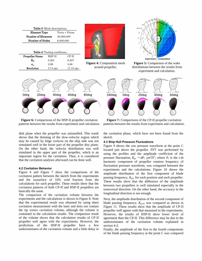
4.2 Cavitation Behavior

Figure 6 and Figure 7 show the comparisons of the

cavitation pattern between the sketch from the experiments

and the isosurface of 10% void fraction from the

calculations for each propeller. These results show that the

cavitation patterns of both CP-II and HSP-II propellers are

basically the same.

The comparison of the cavitation volume between the

experiments and the calculations is shown in Figure 8. Note

that the experimental result was obtained by using sheet

cavitation measurement with the laser and does not contain

the tip vortex cavitation volume, although the volume is

contained in the calculation results. The comparison result

of the volume shows that the calculation results of CP-II

propeller well agree with the experiments. However, the

predictions of the HSP-II propeller have a few

underestimates of the cavitation volume and a little delay in

the cavitation phase, which have not been found from the

sketch.

4.3 Ship Hull Pressure Fluctuations

Figure 9 shows the raw pressure waveform at the point C

located just above the propeller. FFT was performed by

using the profiles and the amplitude coefficient of the

pressure fluctuation, Kpi ＝Pi /n2D

2; where Pi is the i-th

harmonic component of propeller rotation frequency of

fluctuation pressure waveform, was compared between the

experiments and the calculations. Figure 10 shows the

amplitude distribution of the first component of blade

passing frequency, Kp5, for each position and each propeller.

These results show that the difference of the amplitude

between two propellers is well simulated especially in the

transversal direction. On the other hand, the accuracy in the

longitudinal direction is not enough.

Next, the amplitude distribution of the second component of

blade passing frequency, Kp10, was compared as shown in

Figure 11. These results show that the amplitude of CP-II

propeller well agrees with that measured in the experiments.

However, the results of HSP-II show lower level of

agreement than the CP-II. This difference may be due to the

underestimates of the cavitation volume explained in

section 4-2.

Finally, the amplitude of the first to the fourth components

of the blade passing frequency at the point C was compared

0.70.6 0.5 0.40.3

0.2

0.1

Experiment Computation

Figure 4: Computation mesh

around propeller.

Figure 5: Comparison of the wake

distributions between the results from

experiment and calculation.

0deg 20deg 40deg 60deg 80deg 340deg 0deg 20deg 40deg 60deg

Figure 6: Comparisons of the HSP-II propeller cavitation

patterns between the results from experiment and calculation.

Figure 7: Comparisons of the CP-II propeller cavitation

patterns between the results from experiment and calculation.

Table 3: Mesh descriptions.

Element Type Tetra + Prism

Number of Elements 30,000,000

Number of Nodes 6,000,000

Table 4: Testing conditions.

Propeller Name HSP-II CP-II

KT 0.201 0.207

sn 2.99 3.06

Revolution 17.5 rps 17.15 rps

as shown in Figure 12. The calculation results agree with

the experimental results for all the components in a certain

level, rather well for those of CP-II propellers. Therefore,

these results show that the calculation method can be used

to predict the wide range of frequency components of the

hull pressure fluctuation with high accuracy.

4.4 Wavelet Analysis of Pressure Fluctuations

To clarify the relationship between cavitation and pressure

fluctuation on the ship hull in detail, a discrete wavelet

transform was applied to the waveform of the pressure

fluctuation. A discrete wavelet transform is a method to

obtain amplitude information with the temporal resolution

in wider range of frequency than FFT. In this paper, Gabor

Wavelet, written in Eq. (13), was employed as the mother

wavelet for the transform.

𝜓(𝑡) =

1

√2𝜋𝜎2𝑒

−𝑡2

2𝜎2⁄𝑒𝑖𝜔𝑡 (13)

where ω is the angular rate corresponding to the frequency,

and σ is a parameter which affect the frequency resolution.

In this paper, σ = 8 was used.

0

1000

2000

3000

4000

-40 -20 0 20 40 60 80

Cav

ity

Vo

lum

e [

mm

3]

Propeller Angle [deg]

HSP-II HSP-II Exp CP-II CP-II Exp

Figure 8: Comparisons of the cavitation volumes between

the results from experiment and calculation.

Figure 9: The pressure fluctuation waveforms

by the calculation at the point C.

Kp

5K

p1

0

Figure 10: Amplitude distributions of pressure fluctuation.

(1st blade frequency component)

Figure 11: Amplitude distributions of pressure fluctuation.

(2nd blade frequency component)

Figure 12: Amplitude of pressure fluctuation at Point C.

Kp

5K

p1

0

Propeller Angle [deg]

Fre

qu

en

cy[H

z]

Pre

ssu

re [

Pa]

Kp5

Kp10

Kp15

Kp20

Kp25

36 0 36 0 36 0 36

Figure 13: The result of discrete wavelet transform of

pressure fluctuation on CP-II propeller at Point C.

HSP-II CP-II

Pre

ssu

re [

Pa]

0 Propeller Angle [deg] 72

Figure 13 shows the result of a discrete wavelet transform at

point C during the operation of CP-II propeller. In this

graph, the vertical axis indicates frequency component

while horizontal axis time. In this result, high level

amplitude regions such as Kp20 (4th component) and Kp25

(5th component) are around the propeller angle of 30

degrees. The regions are different from the region formed

from Kp5.

To explain the state of cavitation which induces these

higher level components, the distributions of Kp5 and Kp20

were drawn on the isosurface of the 10% void fraction

(Figure 14 and Figure 15). As shown in the figures, Kp5

component is mainly caused by generation and collapse of

the sheet cavitation on the propeller surface.

As for Kp20, the main factor is the collapse of the tip vortex

cavitation around the propeller angle of 30 degrees. The

results match the study suggested by the Konno et al. (2002)

that the higher components of pressure fluctuation are

caused by tip vortex cavitation bursting. In addition, it is

proved that a discrete wavelet transform is useful for

factorial analyses of the pressure fluctuation on the ship

hull.

5 CONCLUSIONS

The computational fluid analysis of the cavitation on the

propeller in the behind-hull condition was performed. From

the calculation result, unsteady cavitation and the pressure

fluctuation induced by the cavitation were evaluated, and

the following conclusions were obtained.

1) The simulation using CFD software achieves high

accuracy in prediction of the cavitation which occurs on the

blade surface and at the tip vortex region.

2) Because the CFD software well simulated unsteady

cavitation with high accuracy, wide range of component-

level of pressure fluctuation on a ship hull induced by the

cavitation was well calculated. This means that the

calculation using CFD software is an effective tool for ship

designing.

3) A discrete wavelet analysis of the calculated pressure

pulse showed that the tip vortex cavitation causes the high-

frequency component of pressure fluctuation. By using this

analysis method, the relationship between cavitation and

pressure fluctuation can be visualized, which will be applied

to more advanced design and development.

REFERENCES

Berger, S., Bauer, M., Druckenbrod, M., and Abdel-

Maksoud, M., (2013), “Investigation of Scale Effects on

Propeller-Induced Pressure Fluctuations by a

Viscous/Inviscid Coupling Approach”, Proc. Third

International Symposium on Marine Propulsors

Egorov, Y., and Menter, F., (2008), “Development and

Application of SST-SAS Turbulence Model in

DESIDER Project”, Advances in Hybrid RANS-LES

Modelling, 261-270

Fujiyama, K., Kim, J-H., Hitomi, D., and Irie, T., (2012),

“Numerical Analysis of Unsteady Cavitation

Phenomena by using RANS Based Methods (in

Japanese)”, Proc. the 16th Cavitation Symposium

Hasuike, N., Yamasaki, S., and Ando, J., (2011),

“Numerical and Experimental Investigation into

Propulsion and Cavitation Performance of Marine

Propeller”, Proc. the 4th International Conference on

Computational Methods in Marine Engineering

Kanemaru, T., and Ando, J., (2013), “Numerical analysis of

cavitating propeller and pressure fluctuation on ship

stern using a simple surface panel method “SQCM”,

Journal of Marine Science and Technology, 18(3), 294-

309

Kawamura, T., (2010), “Numerical Simulation of

Propulsion and Cavitation Performance of Marine

Propeller”, Proc. International Propulsion Symposium

Konno, A., Wakabayashi, K., Yamaguchi, H., Maeda, M.,

Ishii, N., Soejima, S. and Kimura, K., (2002),

“Generation Mechanism of Bursting Phenomena of

Propeller Tip Vortex Cavitation”, Journal of Marine

Science and Technology, 6(4), 181-192

Figure 15: Distributions of Kp20 component

on the 10% void fraction isosurface.

(2nd blade frequency component)

Figure 14: Distributions of Kp5 component

on the 10% void fraction isosurface.

(2nd blade frequency component)

Kurobe, Y., Ukon, Y., Koyama, K., and Makino, M.,

(1983), “Measurement of Cavity Volume and Pressure

Fluctuation on a Model of the Training Ship

‘SEIUNMARU’ with Reference to Full Scale

Measurement (in Japanese)”, SRI Report, 20(6), 395-

429

Menter, F., (1993), “Zonal Two Equation k-ω Turbulence

Models for Aerodynamic Flows”, AIAA 1993-2906

Okuda, K. and Ikohagi, T., (1996), “Numerical Simulation

of Collapsing Behavior of Bubble Clouds (in

Japanese)”, Trans. of JSME(B), 62(603), 3792-3797

Paik, K. J., Park, H-G., and Seo, J., (2013), “URANS

Simulations of Cavitation and Hull Pressure Fluctuation

for Marine Propeller with Hull Interaction”, Proc. Third

International Symposium on Marine Propulsors

Sato, K., Ohshima, A., Egashira, H., and Takano, S.,

(2009), “Numerical Prediction of Cavitation and

Pressure Fluctuation around Marine Propeller”, Proc. the

7th International Symposium on Cavitation

Singhal A. K., Athavale, M. M., Li, H., and Jiang, Y.,

(2002) “Mathematical basis and validation of the full

cavitation model”, Journal of Fluids Eng., 124(3), 617-

624

DISCUSSION

Question from Johan Bosschers

Thank you for your interesting presentation. This is one

of the few papers where the higher harmonic pressure due

to the collapse of cavitating tip vortex seems to be captured

by CFD. I have one remark on the diagram with the wavelet

transform: My experience is that the power in the signal is

better represented if you take the absolute value of the

wavelet coefficients of the Hilbert transform of the time

series. My question is also related with wavelet diagram:

how do these results compare to the results of the

measurements?

Authors’ Closure

Thank you for your observation. In this study, the

amplitudes of pressure fluctuations were compared with the

coefficients only by the FFT analyses, not by the wavelet

analyses. It is because the results of both the wavelet

coefficients and the raw waveform of pressure fluctuations

were not provided from experiments. For the qualitative

observation, this method is useful in its own way. However,

to use it at quantitative analysis, the method needs to be

improved and validated.