Numerical modelling of surcharge loadingOptimisation of surcharge loading to minimise long-term settlements in softsoil

Master’s thesis in Infrastructure and Environmental Engineering

DARKO ASANOVICVALDRIN QYRA

Department of Architecture and Civil EngineeringCHALMERS UNIVERSITY OF TECHNOLOGYMaster’s thesis 2017:85Gothenburg, Sweden 2017

Master’s thesis 2017:85

Numerical modelling of surcharge loading

Optimisation of surcharge loading to minimise long-term settlementsin soft soil

DARKO ASANOVICVALDRIN QYRA

Department of Architecture and Civil EngineeringDivision of Geology & Geotechnics

Chalmers University of TechnologyMaster’s thesis 2017:85

Gothenburg, Sweden 2017

Numerical modelling of surcharge loadingOptimisation of surcharge loading to minimise long-term settlements in soft soilDARKO ASANOVICVALDRIN QYRA

© DARKO ASANOVIC & VALDRIN QYRA, 2017.

Supervisor: Minna Karstunen, Department of Civil and Environmental EngineeringExaminer: Minna Karstunen, Department of Civil and Environmental Engineering

Master’s Thesis 2017:85Department of Architecture and Civil EngineeringDivision of Geology & GeotechnicsChalmers University of TechnologySE-412 96 GothenburgTelephone +46 31 772 1000

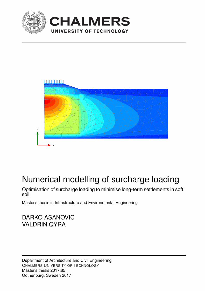
Cover: Visualisation of excess pore water pressure under ground improved embank-ment, constructed in Plaxis 2D.

Typeset in LATEXGothenburg, Sweden 2017

iii

Numerical modelling of surcharge loadingOptimisation of surcharge loading to minimise long-term settlements in soft soilDARKO ASANOVICVALDRIN QYRADepartment of Architecture and Civil EngineeringDivision of Geology & GeotechnicsChalmers University of Technology

AbstractThe purpose of this study was to investigate if secondary compression in soft soilscan be eliminated or minimised by optimisation of surcharge loading. The objec-tive was to perform a numerical analysis of ground improvement with surchargeloading in combination with vertical drains, in order to find the optimal design. Inthis study an embankment was numerically modelled on a homogeneous soft soillayer representative for clay found in Utby, Gothenburg. The numerical modellingwas performed in the software Plaxis 2D and Geosuite Settlement, where the mod-els Creep-SCLAY1S and Chalmersmodel with creep was assessed respectively. Theresults are presented through the analysis of long-term settlements of the embank-ment. Simulations results shows significant differences between the two software.For Creep-SCLAY1S the creep rates could be improved, although the improvementstarts to occur around 1300 years making it difficult to assess the method in practi-cal applications. The simulations in Creep-SCLAY1S also revealed that no swellingoccurred after unloading of surcharge. There is a suspicion regarding the modelformulation in Creep-SCLAY1S, and this due to no swelling was identified and totalsettlements were in general excessive. In Geosuite Settlement the creep could beimproved immediately after the unloading. In general, higher amount of surchargedid not prove to increase the creep improvement ratio in Geosuite. Although, higheramount of surcharge significantly improved the creep rates after unloading. It wasalso noted that the penetration depth of the drains could be reduced up to 40%in Creep-SCLAY1S without affecting the consolidation process. For Geosuite Set-tlement even small changes to the penetration length affected the consolidationprocess.

Keywords: Numerical modelling, Soft soil, Homogeneous soil, Embankment, Pre-fabricated vertical drains, Surcharge loading, Creep improvement ratio, Swelling,Creep-SCLAY1S, Geosuite Settlement.

iv

AcknowledgementsFirstly we would like to to thank our supervisor and examiner Prof. Minna Karstunen,for her guidance and expertise throughout the work. We are extremely grateful forthe opportunity to develop our knowledge in the field, and the opportunity to receivesupport and insights from the highly competent staff at the division of Geology &Geotechnics.

Secondly, we would like to thank the geotechnical staff at Norconsult AB who hasprovided us the practical knowledge concerning the software Geosuite Settlement.They have also showed great interest in our work and contributed with discussionsthat has widen our perspective of the subject.

Lastly, special regards goes out to both our families and friends that motivated andencouraged us on all levels in life, and shaped us to the individuals that we aretoday.

Darko Asanovic & Valdrin Qyra, Gothenburg, June 2017

vi

Contents

List of Figures x

List of Tables xii

Nomenclature xiii

1 Introduction 11.1 Background . . . . . . . . . . . . . . . . . . . . . . . . . . . . . . . . 11.2 Aim and objective . . . . . . . . . . . . . . . . . . . . . . . . . . . . 21.3 Limitations . . . . . . . . . . . . . . . . . . . . . . . . . . . . . . . . 21.4 Method . . . . . . . . . . . . . . . . . . . . . . . . . . . . . . . . . . 3

2 Theory 42.1 Terzaghi’s classical consolidation theory . . . . . . . . . . . . . . . . . 42.2 Secondary compression of soft soil . . . . . . . . . . . . . . . . . . . . 52.3 Relation between secondary compression and overconsolidation ratio . 62.4 Surcharge loading . . . . . . . . . . . . . . . . . . . . . . . . . . . . . 82.5 Prefabricated vertical drains . . . . . . . . . . . . . . . . . . . . . . . 102.6 Geosuite Settlement . . . . . . . . . . . . . . . . . . . . . . . . . . . 122.7 Creep-SCLAY1S . . . . . . . . . . . . . . . . . . . . . . . . . . . . . 142.8 Embankment design . . . . . . . . . . . . . . . . . . . . . . . . . . . 17

3 Method 183.1 General information . . . . . . . . . . . . . . . . . . . . . . . . . . . . 183.2 Embankment and soil geometry . . . . . . . . . . . . . . . . . . . . . 183.3 Simulations cases . . . . . . . . . . . . . . . . . . . . . . . . . . . . . 193.4 Simulations with Geosuite Settlement . . . . . . . . . . . . . . . . . . 203.5 Simulation with Creep-SCLAY1S model . . . . . . . . . . . . . . . . 21

4 Results 244.1 Simulation results from Geosuite Settlement . . . . . . . . . . . . . . 244.2 Simulation results from Creep-SCLAY1S . . . . . . . . . . . . . . . . 28

5 Conclusion 36

Bibliography 38

A Appendix I

viii

Contents

A.1 Derivation of improved permeability (keq) . . . . . . . . . . . . . . . . IA.2 Parameters needed for Chalmersmodel . . . . . . . . . . . . . . . . . IIA.3 Denotation of creep number, r . . . . . . . . . . . . . . . . . . . . . . IIIA.4 Parameters needed for Creep-SCLAY1S . . . . . . . . . . . . . . . . . IV

ix

List of Figures

1.1 Schematic outline of thesis. . . . . . . . . . . . . . . . . . . . . . . . . 3

2.1 Illustration of differences in Hypothesis A and B (Fatahi et al., 2013). 62.2 Creep rate deviation with OCR for β-value 27 (Leoni et al., 2008). . . 72.3 The effects on soil when surcharge loading is used (Almeida and Mar-

ques, 2013). . . . . . . . . . . . . . . . . . . . . . . . . . . . . . . . . 82.4 Effects of surcharging on the rate of secondary compression, Ladd

(1971) presented in Conroy et al. (2015). . . . . . . . . . . . . . . . . 92.5 Data collected from four different papers, results from Shannon Es-

tuary, and Ladd’s mean, upper and lower limit lines (Conroy et al.,2015). . . . . . . . . . . . . . . . . . . . . . . . . . . . . . . . . . . . 10

2.6 Schematic of the effects when combining surcharge load with andwithout vertical drains (Almeida and Marques, 2013). . . . . . . . . . 11

2.7 Illustration of the rheological model with combines phenomenas de-scribing the long term deformations in the soil (Alén, 1998). . . . . . 12

2.8 Validation of Chalmersmodel with laboratory test results (Claesson,2003). . . . . . . . . . . . . . . . . . . . . . . . . . . . . . . . . . . . 13

2.9 Relationship between creep number and vertical effective stress inChalmersmodel. . . . . . . . . . . . . . . . . . . . . . . . . . . . . . . 14

2.10 Illustration of the Creep-SCLAY1S model (Gras et al., 2015). . . . . . 15

3.1 Problem geometry, soil layers and generated mesh. . . . . . . . . . . . 193.2 Illustration of the three different cases simulated. . . . . . . . . . . . 20

4.1 Case II with unloading of AAOS after 2 year. Single drainage withPVDs at full penetration length. . . . . . . . . . . . . . . . . . . . . . 25

4.2 Case II with unloading of AAOS after 2 year. Double drainage withPVDs at full penetration length. . . . . . . . . . . . . . . . . . . . . . 25

4.3 Creep improvement ratio due to surcharge, derived from both drainageconditions in case II using the method proposed by Ladd (1971). . . . 26

4.4 Optimisation of penetration length of the PVDs for single drainage. . 274.5 Optimisation of penetration length of the PVDs for double drainage. 274.6 Results from case I, single- and double drainage conditions with and

without PVDs. . . . . . . . . . . . . . . . . . . . . . . . . . . . . . . 294.7 Case II with unloading of AAOS after 1 year. Single drainage with

PVDs at full penetration length. . . . . . . . . . . . . . . . . . . . . . 30

x

List of Figures

4.8 Case II with unloading of AAOS after 1 year. Double drainage withPVDs at full penetration length. . . . . . . . . . . . . . . . . . . . . . 30

4.9 Creep improvement ratio due to surcharge, derived from both drainageconditions in case II after 1300 years. . . . . . . . . . . . . . . . . . . 31

4.10 Horizontal displacements at embankment toe for different AAOS, caseII for SD conditions. . . . . . . . . . . . . . . . . . . . . . . . . . . . 32

4.11 Horizontal displacements at embankment toe for different AAOS, caseII for DD conditions. . . . . . . . . . . . . . . . . . . . . . . . . . . . 32

4.12 Optimisation of penetration length for single drainage. . . . . . . . . 334.13 Optimisation of penetration length for double drainage. . . . . . . . . 344.14 Horizontal displacements at embankment toe for single drainage when

optimising penetration length of the PVDs. . . . . . . . . . . . . . . . 354.15 Horizontal displacements at embankment toe for double drainage

when optimising penetration length of the PVDs. . . . . . . . . . . . 35

xi

List of Tables

3.1 Parameters needed in Chalmersmodel with creep addendum. . . . . . 213.2 Parameters needed for Creep-SCLAY1S-model used in Plaxis 2D. . . 223.3 Staged construction as loading for the embankment. . . . . . . . . . . 23

A.1 Calculation of improved permeability to represent the PVDs in the soil. IA.2 Parameters needed for sand layer using Janbu-sand model. . . . . . . IIA.3 Model parameters the clay layer using Chalmersmodel with creep

addendum. . . . . . . . . . . . . . . . . . . . . . . . . . . . . . . . . . IIA.4 Calculated parameters for Chalmersmodel with creep addendum. . . . IIIA.5 The additional initial stress state parameters for the soil layers. . . . IVA.6 Isotropic parameters used for the clay layer. . . . . . . . . . . . . . . IVA.7 Anisotropic parameters used for the clay layer. . . . . . . . . . . . . . IVA.8 Destructuration parameters used for the clay layer. . . . . . . . . . . IVA.9 Viscous parameters used for the clay layer. . . . . . . . . . . . . . . . IV

xii

Nomenclature

AbbrevationsAAOS Adjusted Amount of SurchargeCC Center to CenterCL Center LineCSR Constant Rate of StrainCSS Current Stress StateDD Double DrainageEOP End of Primary ConsoldationIL Incremental LoadingNCS Normally Consolidated SurfaceOCR Overconsolidation ratioPOP Pre Overburden PressurePV D Prefabricated Vertical DrainsSD Single DrainageU Degree of Consolidation

Greek Symbolsα Adhesion factorα0 Initial value of ααd Deviatoric fabric tensorβ Creep exponentχ Degree of bondingχ0 Initial value of χδ∗ Modified compression indexδ∗ Modified compression indexεpd Plastic deviatoric strainεpv Plastic volumetric strainη Stress ratio

xiii

Nomenclature

η0 Initial stress ratioγ Unit weight of soilγw Unit weight of water[kN/m3]γemb Unit weight of embankmentκ Slope of recompression curveκ∗ Modified swelling indexΛ Visco-plastic multiplierµ∗ Modified creep indexµ∗i Modified intrinsic creep indexω Absolute rate of rotation of yield surfaceωd Relative effectiveness of plastic strainσ′ Effective stress [kPa]σ′p Pre-consoldiation pressure [kPa]σ′vf Final effective stress [kPa]σ′vs Effective stress under surchargeτ Reference Timeξ Absolute rate of destructurationξd Relative effectiveness of destructuration rate

Roman Symbolse Rate of change of void ratioee Elastic rate of change of void ratioUh Average degree of horizontal consolidationa0 Stress factora1 Stress factorb1 Stress factorbo Stress factorCα Secondary compression indexCc Compression indexCh Coefficient of consolidation in horizontal direction [m2/year]Cs Swelling indexcv Coefficient of vertical consolidation [m2/year]de Equivalent drainange diamater [m]dw Diameter of drainec Rate of change of voids due to creep

xiv

Nomenclature

H Thickness [m]hf Height of embankment [m]hfs Height of surcharge [m]k Hydraulic conductivity [m/s]kh Hydraulic conductivity in horizontal direction [m/s]ks Hydraulic conductivity in smear zone [m/s]l Drainage length [m]M Compression modulus [kPa]M ′ Stress-dependent component modulus for stress ≥ σ′L

ML Component modulus between pre-consolidated pressure and σ′LMo Component modulus in over-consolidated statep′ Mean effective stress [kPa]p′p Size of normal consolidation surface in p’-q plane [kPa]p′eq Size of current stress surface in p’-q plane [kPa]p′mi Size of intrinsic yield curve in p’-q plane [kPa]p0 In-situ effective mean stress [kPa]qw Discharge capacity [l/s]R Time resistancer Creep numbert TimeTh Time factor in horizontal directionTv Time factor in vertical directionu Pore pressure [kPa]z Elevation head [m]

xv

1Introduction

This chapter provides a background to the study followed by the aim and objectives.Furthermore, the demarcations are specified and the method’s section gives a briefdescription of how the study was performed. Lastly, this chapter presents the outlineof the report.

1.1 Background

The urbanisation trend poses several construction challenges for engineers duringthe upcoming decades. More than half of the worlds population currently residesin urban areas (Kalmykova et al., 2015). By year 2050 an increase in populationof 20-30% is expected in the urban areas worldwide. In order to meet this trenda large share of the urban development still needs to be constructed (Swillingandand Robinson, 2013). In synergy with the growing population in cities, line infras-tructure connections between cities and other countries is crucial for establishing asustainable and attractive transport system. Gothenburg city is the second largestcity in Sweden that is currently undergoing major urbanisation. The city is locatedin the Western part of Sweden and has currently two large urban developmentsplanned, Älvstaden and Västsvenska paketet (Mehner, 2017). Urban areas locatedin coastal regions are facing difficulties in locating good quality sites for new de-velopment. Gothenburg is one of the cities that is geologically located in a areadominated by soft soils. Generally, soft soils are prone to settlements and stabilityissues that geotechnical engineers will be facing in the near future.

The properties of soft soil is determined by various factors, type of deposition andgeographic location of soil minerals has a large impact on the geotechnical charac-teristics. Glacial and postglacial clay deposits are common in the Nordic countries,Canada and Northern parts of the US. Soft soil deposits are often associated withlow shear strength and high sensitivity, where the sensitivity can exceed 50. Thevolcanic clay deposits in Mexico City are characterised by the high water contentand are highly compressible with large secondary compression. The Bangkok clay isgenerally uniform although intersection by fine cracks are present. The sensitivityis low and the compressibility of the clay is high (Knappett and Craig, 2012). In

1

1. Introduction

short, the characteristics of the soft soils deposits varies by location and should beanalysed separately for detailed information regarding soil properties.

Kansai International Airport is one example of a project initiated where new landhas been reclaimed. The project comprises of two islands, island I and II, locatedin Osaka Bay (Japan). The project has received large attention in geotechnical pa-pers due to its large scale and complexity. Both island I and II are continuouslysettling, predictions indicate that both will be under sea level by end of the thiscentury (Mesri and Funk, 2015). The difficulties with these large scale projects isusually the settlement predictions. Site investigations and laboratory consolidationtests has not proven to be give enough information for the settlement predictions.Secondary compression can also contribute significantly to the settlements even dur-ing the primary consolidation, although at end of the primary consolidation processsecondary compression is more evident (Puzrin et al., 2010).

Due to the complexity of fully understanding soft soil behaviour, researchers has pro-posed several constitutive models in order to receive more accurate settlement andstability predictions. One of the most recently proposed models is Creep-SCLAY1S,a model developed to predict the long-term settlements in soft sensitive clays. In ad-dition to the isotropic parameters, the model also takes into account the anisotropy,destructuration and viscosity of the soft soil. Numerical modelling enables advancedembankment designs to be analysed. The embankment will be modelled in Plaxis2D (using Creep-SCLAY1S as a model) and the commercial software Geosuite.

1.2 Aim and objective

The aim of this thesis is to investigate if secondary compression in soft soils canbe eliminated or minimised by optimisation of surcharge loading. The objective isto perform a numerical analysis of ground improvement with surcharge loading incombination with vertical drains, in order to find the optimal design.

1.3 Limitations

In this thesis a homogeneous clay layer has been analysed. The soil parameters arebased on the Utby clay and has earlier been derived and evaluated at Chalmers Uni-versity of Technology. The selected ground improvement methods are less commonin the Scandinavian countries and was particularly chosen for that reason.

2

1. Introduction

1.4 Method

After the problem identification the investigation proceeded with a literature reviewregarding surcharge loading, vertical drains and numerical modelling. Further on,a review of the Creep-SCLAY1S model and Geosuite Settlement was done in orderto understand how the models works and what parameters are included. Afterthe literature study was completed, a set of parameters was chosen to perform thesimulations in the numerical tools. Three different cases was set to realise the aimof the thesis, where several simulations was made to find the optimal solution ofsurcharge load and penetration depth of the drains. In the last part of this studyan analysis of the results and conclusion was conducted. Figure 1.1 schematicallysummarises the structure of this paper.

Problem identification

Literature review

Parameter setup

Simulations

Case Ⅰ

Case Ⅱ

Case Ⅲ

Analysis

Conclusion

Figure 1.1: Schematic outline of thesis.

3

2Theory

In the following sections, relevant literature and knowledge that concerns the mas-ter thesis is presented. Initially the consolidation theory of soft soils is presented,followed by the relevant ground improvement methods used in the thesis. Lastly,the theory for the constitutive models are presented.

2.1 Terzaghi’s classical consolidation theory

Primary consolidation is a time-dependent volumetric deformation of soils with lowpermeability. This occurs due to application of a load on the surface (i.e. change ineffective stress), which immediately results in an increase of pore water pressure andbuild up of excess pore water pressure in the soil. As a result, the hydraulic gradientincreases and as a consequence drainage of the pore water in the soil occurs, untilthe equilibrium is reached, with deformations keep developing in the soil (Knap-pett and Craig, 2012). The mathematical formulation for calculating the degreeof consolidation at any time t, was developed by Terzaghi (1943). The theory isvalid for one-dimensional consolidation calculations and is widely accepted. TheEquation 2.1 presents the formulation.

Tv = cvH2 · k (2.1)

where the Tv is the time factor in vertical direction, H is the thickness of the soillayer [m], k is the hydraulic conductivity [m/s]. The coefficient of consolidation invertical direction, cv [m2/s], is expressed as Equation 2.2.

cv = k ·Mγw

(2.2)

whereM represents the compression modulus [kPa] and γw is the unit weight of thewater [kN/m3].

The classical consolidation theory proposed by Terzaghi (1923) relies on the uniquerelationship between effective stress and time independent strain. Additionally, themodulus and the permeability of the soil is assumed to be constant with time.

4

2. Theory

Equations 2.3 & 2.4 presents the theory in two different formats,

∂u

∂t= M

γ

∂

∂z

(k · ∂u

∂z

)or (2.3)

∂u

∂t= cv

∂2u

∂z2 (2.4)

Equation 2.4 is based on several assumptions where the first assumes fully satu-rated and homogeneous soil. The strain and pore water flow is assumed to beone-dimensional and Darcy´s law is valid. The change in pore water pressure isequal to the change in effective stress, the equation also assumes that the pore wa-ter and soil particles are incompressible. The last assumption is that the strain isstrictly dependent on the effective stress.

2.2 Secondary compression of soft soil

Secondary compression, also known as creep, is generally studied via from one di-mensional consolidation tests conducted in the laboratory. The laboratory tests isusually presented in a time-compression curve where initial and primary consolida-tion can be obtained. The initial compression occurs due to a load is applied to thesoil and immediate settlements are detected. As mentioned, primary consolidationoccurs due to dissipation of excess pore water pressure and is therefore the driv-ing force that causes the settlements. In contrast, a clear definition of secondarycompression is yet not established and creep is still a challenge in geotechnical engi-neering. However, different theories has been presented to resolve the advancementof creep in soft soils.

One of the theories refer to the micro- and macro-fabric of the soft soils. Observa-tions of the anisotropic fabric of soft soils shows low internal porosity for the clayminerals (Navarro and Alonso, 2001). The range of the porosity varies within 10-100nm where water could be in a adsorbed state. The amount of adsorbed water isdetermined by the specific surface of the soil particles and is called microstructuralwater. The microstructural water has different properties from the free water inclay minerals when considering the aspects of structure and thermodynamics. Theconcept of this theory is to analyse the local water transfer from the mictrostructuralvoids to the macrostructurals voids of the soft soil body. Therefore, understandingchanges in volume over time in the microscale can provide knowledge of deformationsin the macroscale. However, until this equilibrium is reached, the long-term creepdeformation are continuously occurring (Navarro and Alonso, 2001). Other theoriespropose that creep to be dependent on various factors where chemical, geomicrobi-ological and mechanical processes has great effect (Mitchell and Soga, 2005).

Further implications follows when determining creep in practical applications, as indetermining the long-term settlements. These implications exists since disagreement

5

2. Theory

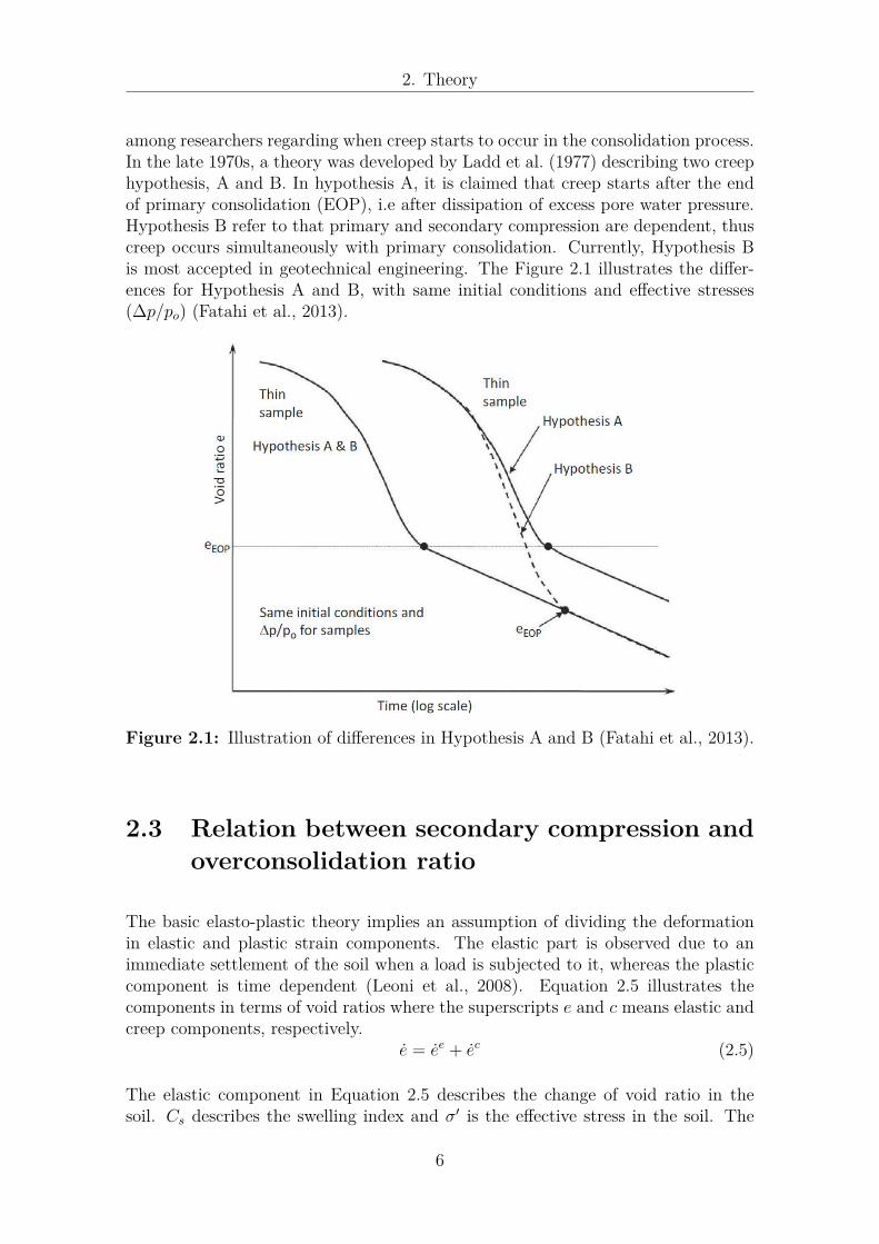
among researchers regarding when creep starts to occur in the consolidation process.In the late 1970s, a theory was developed by Ladd et al. (1977) describing two creephypothesis, A and B. In hypothesis A, it is claimed that creep starts after the endof primary consolidation (EOP), i.e after dissipation of excess pore water pressure.Hypothesis B refer to that primary and secondary compression are dependent, thuscreep occurs simultaneously with primary consolidation. Currently, Hypothesis Bis most accepted in geotechnical engineering. The Figure 2.1 illustrates the differ-ences for Hypothesis A and B, with same initial conditions and effective stresses(∆p/po) (Fatahi et al., 2013).

Figure 2.1: Illustration of differences in Hypothesis A and B (Fatahi et al., 2013).

2.3 Relation between secondary compression andoverconsolidation ratio

The basic elasto-plastic theory implies an assumption of dividing the deformationin elastic and plastic strain components. The elastic part is observed due to animmediate settlement of the soil when a load is subjected to it, whereas the plasticcomponent is time dependent (Leoni et al., 2008). Equation 2.5 illustrates thecomponents in terms of void ratios where the superscripts e and c means elastic andcreep components, respectively.

e = ee + ec (2.5)

The elastic component in Equation 2.5 describes the change of void ratio in thesoil. Cs describes the swelling index and σ′ is the effective stress in the soil. The

6

2. Theory

dot in seen in ee and σ notes the equation is time-dependent. The negative sign inEquation 2.6 follows from the conventional signs in soil mechanics where compressionis positive.

ee = − Csln 10

σ′

σ′(2.6)

The plastic component is due to the viscous behaviour of soft soil, and thereforethe deformations are time-dependent. Equation 2.7, also referred as the power law,illustrates the phenomena where Cα and Cc are the secondary compression indexand compression index, respectively, β is the creep exponent and τ is the referencetime.

ec = − Cατ ln 10

(σ′

σ′p

)βwith β = Cc − Cs

Cα(2.7)

The ratio (σ′/σ′p) is also referred as the inverse of the overconsolidated ratio (OCR).In Leoni et al. (2008), the relationship between creep rate and OCR with typicalcompression index values, which results into β=27, is demonstrated. In Figure 2.2the void ratio is plotted against the effective stress with different OCR-values.

Figure 2.2: Creep rate deviation with OCR for β-value 27 (Leoni et al., 2008).

As seen in Figure 2.2, the creep rate is very high for the case of OCR less than one.Moreover, the creep rate is high for soils with OCR values around one and almostnegligible for OCR higher than 1.3 (Leoni et al., 2008). This feature can potentiallybe exported in the design of surcharge loading in order to minimise or eliminatecreep deformations.

7

2. Theory

2.4 Surcharge loading

Generally, there are two types of issues addressed when poor soil quality is en-countered; stability and settlement problems. Therefore, different types of groundimprovement techniques are used to control these issues and to strengthen the soil.There are methods available to improve both the stability and control settlements.It should be stressed that the soil properties at different locations should be analysedindividually to find a suitable solution for ground improvement.

By applying a temporary surcharge load hfs in excess of the final construction loadshf the rate of settlement through primary consolidation is accelerated. Figure 2.3shows the procedure in detail, where the total theoretical settlements (∆hf ) areachieved significantly faster with higher surcharge load at the equal time (t1) (Almeidaand Marques, 2013).

Figure 2.3: The effects on soil when surcharge loading is used (Almeida and Mar-ques, 2013).

Unlike many other materials, soft soil experience significant volume changes undersurcharge load. When unloading the surcharge and then reloading with the con-struction load, the goal is to minimise the change in volume. This to reduce thepotential structural distresses in the future caused by the secondary compression inthe soil (Tewatia et al., 2007). In Figure 2.3 shows that at time t1 when the sur-charge is removed, the settlement stabilisation rate is accelerated and thereby thesecondary compression settlements are minimised. The removal of the surchargecan result in a rebound effect where the soil swells, however this phenomena is oftenneglected in the field (Almeida and Marques, 2013).

To achieve reduction in secondary compression by surcharge loading, the creep rateof Cα needs to be improved. As shown in Figure 2.4, this usually can be achievedafter removal of the higher surcharge load. The soil swells for a certain durationafter the surcharge has been removed. After the swelling ends the secondary com-pression resumes under a new constant effective stress. The secondary compression

8

2. Theory

tP = End of primary

tR = Removal of surcharge

tS = Start of secondary

εv

Log t

C1

1C’

Figure 2.4: Effects of surcharging on the rate of secondary compression, Ladd(1971) presented in Conroy et al. (2015).

now occurs at a lower rate of C ′α than it would without surcharge loading. This be-haviour proves that the longer time the surcharge loading is left in place, the moredrawn-out time for swelling is needed before secondary compression with a lowercompression rate continues Cα (Balasubramaniam et al., 2010). In the paper pre-sented by Balasubramaniam et al. (2010) recommendations are given for the degreeof consolidation (DOC) when preloading with and without PVDs. Generally, theDOC should be higher than 90% or even 95% in order to ensure that no primarysettlements are added to the secondary settlements, and thus contributing to higherpost-construction settlements.

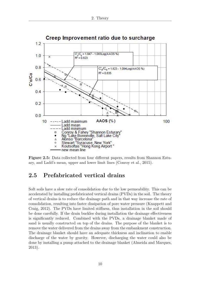
Recent work by Conroy et al. (2015) has investigated the required amount of sur-charge loading needed to improve the rate of secondary compression. The analysiswas based on the procedure of long term oedometer tests at various levels of sur-charge loading. The paper concluded that Ladd’s method, as cited in Conroy et al.(2015) may be used as a good estimate in design of embankments on soft soils. InEquation 2.8 the adjusted amount of surcharge can be calculated, where σ′vs is theeffective stress under surcharge, and σ′vf is the final effective stress after the sur-charge loading has been removed. Ladd (1971) discovered that the ratio of C ′α toCα is related to the level of surcharge loading applied to the soil. The relationshipbetween C ′α/Cα and the adjusted amount of surcharge, (AAOS) is presented in Fig-ure 2.5. As can be seen, higher amount of AAOS gives better creep improvementratios.

AAOS =σ′vs − σ′vfσ′vf

(2.8)

9

2. Theory

Figure 2.5: Data collected from four different papers, results from Shannon Estu-ary, and Ladd’s mean, upper and lower limit lines (Conroy et al., 2015).

2.5 Prefabricated vertical drains

Soft soils have a slow rate of consolidation due to the low permeability. This can beaccelerated by installing prefabricated vertical drains (PVDs) in the soil. The theoryof vertical drains is to reduce the drainage path and in that way increase the rate ofconsolidation, resulting into faster dissipation of pore water pressure (Knappett andCraig, 2012). The PVDs have limited stiffness, thus installation in the soil shouldbe done carefully. If the drain buckles during installation the drainage effectivenessis significantly reduced. Combined with the PVDs, a drainage blanket made ofsand is usually constructed on top of the drains. The purpose of the blanket is toremove the water delivered from the drains away from the embankment construction.The drainage blanket should have an adequate thickness and inclination to enabledischarge of the water by gravity. However, discharging the water could also bedone by installing a pump attached to the drainage blanket (Almeida and Marques,2013).

10

2. Theory

The theory of calculating the average degree of horizontal consolidation Uh in practi-cal applications with drains was introduced by Hansbo (1981). The formula assumesequal vertical strain and does not consider the vertical drainage of the natural soil.The last assumption may give unrealistic results for thin soft soil layers with drainagelayers both on top and bottom (Kirsch and Bell, 2013). It can be calculated at adepth, z, and at time, t, from 2.9,

Uh = 1− exp(− 8Th

µ

)(2.9)

where Th is the time factor for horizontal consolidation and µ is accounting for boththe smear and well resistance in the drain. The equations for Th and µ are presentedas:

Th = cht

d2e

, (2.10)

µ = ln ns

+ khks

ln(s)− 34 + π

2l2kh3qw

(2.11)

where ch represents the coefficient of consolidation in horizontal direction, de repre-sents the equivalent drainage diameter of the drain dependent on the c-c distance,and t is equal to time presented in Equation 2.10. In Equation 2.11, n = de

dw, where

dw is the diameter of the drain, s = dsdw

where ds is the diameter of the smear zone.The hydraulic conductivity values, kh and ks, shows the conductivity of the soilin horizontal plane and the smear zone respectively. The l parameter determinesthe drainage length and qw determines the discharge capacity of the vertical drains.The first part of the equation, including the constant −3

4 , accounts for the smearzone, whereas the second part presents the well resistance in the drain (Chai et al.,2001). In general the PVDs are combined with surcharge load to increase the rateof settlements in the natural subsoil. In some cases where the soft soil profile isthick with low permeability, it is reasonable to use the combination of the two soilimprovement methods (Brand and Brenner, 1981). In Figure 2.6 the enhanced effi-ciency of the vertical drains are schematically illustrated, proving that settlementsoccur at a faster pace.

Figure 2.6: Schematic of the effects when combining surcharge load with andwithout vertical drains (Almeida and Marques, 2013).

11

2. Theory

Figure 2.7: Illustration of the rheological model with combines phenomenas de-scribing the long term deformations in the soil (Alén, 1998).

2.6 Geosuite Settlement

The finite element engine used in Geosuite Settlement is based on the rheologicalmodel proposed by Alén (1998). The theory of the model is based on the classicalone-dimensional consolidation theory presented by Terzaghi (1923). Moreover, de-velopment and validation of the Chalmersmodel implemented in Geosuite have beendone when analysing creep in the soft soils. This simple model is governed by thethree phenomena; consolidation (A), elastic and plastic deformation (B) and creepdeformation (C). The consolidation process accounts for the pore water dissipationand also restricts the strain rate. Elastic and plastic strains in the soil are detectedby the model due to an increase of effective stress and the creep strain is occurringdue to a constant effective stress level over time. The Figure 2.7 below illustrates themodel with the different phenomenas. The combined effects of the three phenomenaon soil, considering the deformations with time, can be derived from Equation 2.12.

∂εz∂t

= − 1M· ∂u∂t

+ 1R

(2.12)

where M is the oedometer modulus of the soil, u is the pore water pressure, trepresents the time and R is the time resistance.

When considering the change in pore water pressure over time (∂u/∂t) similar equa-tion proposed in Terzaghis consolidations theory can be used, except from the creepaddendum. In Equation 2.13 the change in pore pressure with respect to time ispresented.

∂u

∂t= M · kz

γw

∂2u

∂z2 + 1R

(2.13)

where γw represents the unit weight of the water, k the permeability at differentdepth and the creep addendum is the ratio 1/R.

The settlements parameters in Geosuite Settlement are based on three compression

12

2. Theory

Figure 2.8: Validation of Chalmersmodel with laboratory test results (Claesson,2003).

resistance modulus; Mo, ML and M ′. These parameters are derived from constantrate of strain oedometer tests. Moreover, the results are validated in the manner thatthe σ′−M -diagram shown in figure 2.8 matches the CRS laboratory tests (SwedishStandard Institute, 1991). According to Claesson (2003), this method is more suit-able than the older Swedish practice when doing settlement calculations in soft soil.This due to that the Chalmersmodel does an adaption of the oedometer modulesaround the preconsolidation pressure from M0 to ML. This phenomena could beseen in Figure 2.8.

Further on, the stress factors ao and a1 could be set as 0.8 and 1.0 respectively. Inorder to calculate the oedometer modules, M, around the preconsolidation pressure,empirical formula’s have been denoted and they are illustrated in Equation 2.14.

M =

M0 if σ′v < a0σ

′c

M0 + (ML −M0) σ′v−a0σ′ca1σ′c−a0σ′c

if a0σ′c ≤ σ′v < a1σ

′c

ML if a1σ′c ≤ σ′v < σ′L

ML +M ′(σ′v − σ′L) if σ′v ≥ σ′L

(2.14)

Additionally, an extension was made to take the creep factor into account. Whenconsidering the creep supplement, five more parameters are needed to calculate thetime resistance R, which could be found in Equation 2.13. Similar to the oedometermodules, Claesson (2003) claims that the creep number, rs, is a better estima-tion when considering the creep behaviour of soft soil than secondary coefficient ofconsolidation, Cα. In Chalmersmodel, the creep number is denoted from the fourremaining parameters r0, r1, b0 and b1. The stress parameter b1 could be set toeither 1.0 or 1.1, although the most common value is 1.1. In Figure 2.9, the creepnumber is described according to Chalmersmodel and how it is calculated based on

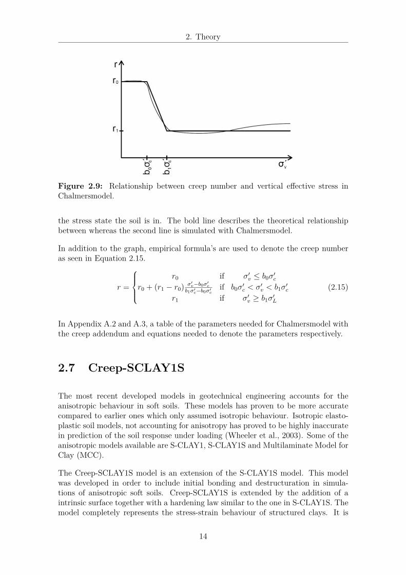
13

2. Theory

Figure 2.9: Relationship between creep number and vertical effective stress inChalmersmodel.

the stress state the soil is in. The bold line describes the theoretical relationshipbetween whereas the second line is simulated with Chalmersmodel.

In addition to the graph, empirical formula’s are used to denote the creep numberas seen in Equation 2.15.

r =

r0 if σ′v ≤ b0σ

′c

r0 + (r1 − r0) σ′v−b0σ′cb1σ′c−b0σ′c

if b0σ′c < σ′v < b1σ

′c

r1 if σ′v ≥ b1σ′L

(2.15)

In Appendix A.2 and A.3, a table of the parameters needed for Chalmersmodel withthe creep addendum and equations needed to denote the parameters respectively.

2.7 Creep-SCLAY1S

The most recent developed models in geotechnical engineering accounts for theanisotropic behaviour in soft soils. These models has proven to be more accuratecompared to earlier ones which only assumed isotropic behaviour. Isotropic elasto-plastic soil models, not accounting for anisotropy has proved to be highly inaccuratein prediction of the soil response under loading (Wheeler et al., 2003). Some of theanisotropic models available are S-CLAY1, S-CLAY1S and Multilaminate Model forClay (MCC).

The Creep-SCLAY1S model is an extension of the S-CLAY1S model. This modelwas developed in order to include initial bonding and destructuration in simula-tions of anisotropic soft soils. Creep-SCLAY1S is extended by the addition of aintrinsic surface together with a hardening law similar to the one in S-CLAY1S. Themodel completely represents the stress-strain behaviour of structured clays. It is

14

2. Theory

Figure 2.10: Illustration of the Creep-SCLAY1S model (Gras et al., 2015).

basically a rate dependent model that accounts for changes in fabric arrangementand bonding (Karstunen et al., 2013).

The intrinsic yield surface is denoted as p′mi, Current Stress Surface (CSS) as p′eqand Normal Consolidation Surface (NCS) as p′p, and are illustrated in Figure 2.10.Equation 2.16 is referred as the volumetric hardening law and accounts for theevolution of the volumetric creep strains. The p′p value specifies the size of NormalConsolidated Surface and is a boundary for the interval between the small andlarge creep strains. λ?i the modified compression index and κ? the modified swellingindex (Sivasithamparam et al., 2015).

∆p′p =p′p

λ?i − κ?∆εpv (2.16)

The inner ellipse specifies the Current Stress Surface and can be derived from Equa-tion 2.17, where it represents the current state of the effective stress (Sivasitham-param et al., 2015).

p′eq = p′2 + (q − αp′)2

(M2 − α2)p′ (2.17)

Grimstad et al. (2010) presented the visco-plastic multiplier which accounts for creepbehaviour in soft soils. The multiplier is presented in Equation 2.18 where µ?i is theintrinsic creep index and is usually derived from IL oedometer tests. Although, theterm (M2

c −α20)/(M2

c − η20) is added to the equation to provide correct creep strains

with the corresponding measured volumetric creep strain rate under Oedometer

15

2. Theory

conditions (Sivasithamparam et al., 2015).

Λ = µ?iτ

(peq

(1 + χ)p′mi

)λ?i−κ?

µ?i M2

c − α20

M2c − η2

0(2.18)

The Mc-value which denotes the critical state slope can be derived from triaxialcompression tests. The parameters α0 and η0 refers to the initial inclination ofthe yield surface and stress ratio corresponding to KO Consolidation, respectively.Including the visco-plastic multiplier the analysis can extend above the critical stateline and enter the dry side similarly to the MCC model. For overconsolidated soilsthis can in many cases result in a higher undrained shear strength. An associatedflow rule is assumed in the Creep-SCLAY1S model where creep strain rate is definedby the visco-plastic multiplier shown in Equation 2.19.

εcij = Λ∂p′eq∂σ′ij

(2.19)

The hardening laws similar to the S-CLAY1S model are as mentioned included inthe model, with the plastic strains are exchanged with creep strains. The firsthardening law represents the increased size of the intrinsic yield surface p′mi seen inEquation 2.20.

p′mi = vp′miλi − κ

εcv (2.20)

Although, the first hardening law in Equation 2.20 can be reduced to MCC-analysisfrom Equation 2.16 if destructuration is ignored. The second hardening law waspresented by Wheeler et al. (2003) and is presented in Equation 2.21. The hardeninglaw describes the change in the orientation of the yield surface, also known as therotational hardening law.

αd = ω

[(3η4 − αd

)⟨εcv⟩

+ ωd

(η

3 − αd)εcd

](2.21)

In the equation, η represents the stress ratio, ω and ωd are model constants. ω deter-mines the absolute rate of rotation of the yield surface, and ωd controls the relativeeffectiveness of plastic strains. The third hardening law considers the degradation ofinter-particle bonding with plastic straining. The bonding parameter χ is introducedand gets reduced to zero with an increase in plastic strains. Change in bonding χcan be derived from Equation 2.22.

dχ = ξ[(0− χ)|εcv|+ ξd(0− χ)εcd] = −ξχ(|εcv|+ ξddcd) (2.22)

The bonding paramter χ is dependent of the two soil properties, ε and εd which gov-erns the absolute rate of destructuration and relative effectiveness of plastic strainsduring bond degradation. In Creep-SCLAY1S the critical state M is included as a

16

2. Theory

function of a lode angle. The function for the critical state is given by Equation 2.23,m represents the ratio between critical state slope in extension and the critical statein compression.

M(θ) = Mc

( 2m4

1 +m4 + (1−m4) sin 3θα

) 14 (2.23)

2.8 Embankment design

The typical embankments constructed is Sweden are based on the guidelines pur-suant to the Transport Administration (Trafikverket). Embankments should bebuilt in the manner that no nearby construction is affected. Additionally, no com-promises should be taken which could impact the stability of the construction orthe embankment. If there is risk for environmental impact, embankments should beconstructed according to different categories described in Alm (2000).

The standardised road widths in Sweden for a 2 + 2 highway, can be designed basedon document Alm (2000). The following dimensions are assumed for the road widthin one direction, two lanes is equal to 7.5 meters, one verge of 3 meters, two outerhard strip edges of 0.5 meters. Summarising these, a total crown width should atleast be 11 meters.

Slopes in Sweden are usually 1:3, these slopes puts drivers at risk for overturning.Flatter slopes has been recommended, 1:4 to 1:6, and even flatter can reduces therisk of overturning significantly. High embankment heights can be built with bothsteeper or flatter inclinations depending on how much space can be allocated for theroad (Alm, 2000).

17

3Method

The third chapter is concerned with the methodology for this study. All relevantinformation regarding how the analysis was performed can be found in this chapter.Simulations was done in Geosuite Settlement and Plaxis 2D, where access was givento the yet commercially unavailable Creep-SCLAY1S model.

3.1 General information

The idealised embankment was analysed on Utby clay and is located in the out-skirts of Gothenburg. In general, the Utby clay shows similar characteristics withthe soft soils found in the Gothenburg region. Researchers at Chalmers Universityof Technology are currently using the Utby site for soil testing. The available lab-oratory tests for the Utby clay are Odeometer tests, both incremental loading (IL)and constant rate of strain (CRS), and triaxial tests. The laboratory tests have beenconducted from mini-block samples and piston samples and validation of the param-eters have been done for both types by Karlsson et al. (2016). In this thesis, datafor the two models used have been derived from the same IL tests extracted at eightmeters depth. The soil under the embankment was improved with prefabricatedvertical drains. The drains are assumed to be 100 mm wide and 4 mm thick. Thearrangement of the prefabricated vertical drains was set to a square pattern with 2m of centre-to-centre distance. To represent the PVDs in the clay, improvement ofpermeability accordingly to Chai et al. (2001) has been performed. The improve-ment of permeability is a simplification to assess PVDs in 1D- and 2D-analysis. InAppendix A.1 the calculations are presented. On top of the embankment surchargeloading was applied to increase the rate of primary consolidation, and thus increasethe undrained shear strength and minimise creep.

3.2 Embankment and soil geometry

The embankment was symmetric and therefore only the right half was analysed.The dimensions of the embankment was 14 meters wide, 2 meters high and it was

18

3. Method

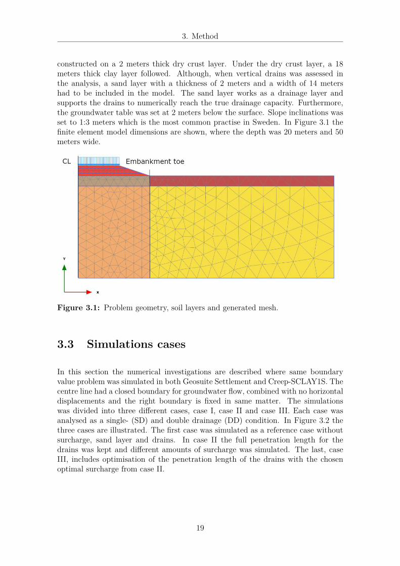
constructed on a 2 meters thick dry crust layer. Under the dry crust layer, a 18meters thick clay layer followed. Although, when vertical drains was assessed inthe analysis, a sand layer with a thickness of 2 meters and a width of 14 metershad to be included in the model. The sand layer works as a drainage layer andsupports the drains to numerically reach the true drainage capacity. Furthermore,the groundwater table was set at 2 meters below the surface. Slope inclinations wasset to 1:3 meters which is the most common practise in Sweden. In Figure 3.1 thefinite element model dimensions are shown, where the depth was 20 meters and 50meters wide.

Figure 3.1: Problem geometry, soil layers and generated mesh.

3.3 Simulations cases

In this section the numerical investigations are described where same boundaryvalue problem was simulated in both Geosuite Settlement and Creep-SCLAY1S. Thecentre line had a closed boundary for groundwater flow, combined with no horizontaldisplacements and the right boundary is fixed in same matter. The simulationswas divided into three different cases, case I, case II and case III. Each case wasanalysed as a single- (SD) and double drainage (DD) condition. In Figure 3.2 thethree cases are illustrated. The first case was simulated as a reference case withoutsurcharge, sand layer and drains. In case II the full penetration length for thedrains was kept and different amounts of surcharge was simulated. The last, caseIII, includes optimisation of the penetration length of the drains with the chosenoptimal surcharge from case II.

19

3. Method

Figure 3.2: Illustration of the three different cases simulated.

3.4 Simulations with Geosuite Settlement

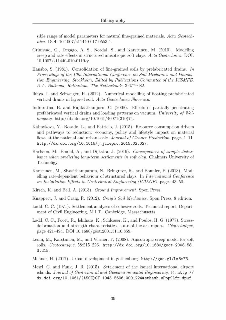
In Geosuite Settlement simulations was performed with the soil model called Chalmerswith creep addendum, and the permeability model log based strain. The parameterswere derived from the CRS-tests conducted from STII-piston samples. In Table 3.1a summary of the parameters needed for Chalmersmodel with creep addendum ispresented. The soil model used for the sand layer was Janbu-sand model. The pa-rameters used for the sand was assumed to some reasonable values. In Appendix A.2the parameters needed and used in Geosuite Settlement for the sand are presented.In Geosuite Settlement the embankment was simulated as a load and it was buildinstantly. On top of the embankment, various of surcharge loads was simulated.The surcharge load was consolidated for two years and then removed.

Division of the layers with respective parameters was set as illustrated in Table A.3.The unit weight of water was set as 10 kN/m3 and the bulk modulus as 2× 106

kN/m2. The embankment was simulated as a constant line load and the surchargeis simulated in same matter. The tolerance factor that determines the range of errorallowed was set as 0.0003 and maximum iteration per step was set to 1000.

20

3. Method

Table 3.1: Parameters needed in Chalmersmodel with creep addendum.

Term in the model Unit Explanationγ kN/m3 Unit weight of materialM0 kN/m2 Oedometer modulus at stress level > a0 σ

′c

ML kN/m2 Oedometer modulus at stress level between a1 σ′L

M ′ - Oedometer modulus at stress level < σ′La0 - Stress factor ≥ 1a1 - Stress factor ≤ 1σ′c kN/m2 Preconsolidation pressureσ′L kN/m2 Preconsolidation pressuretref year Reference time, often assumed to be -1 dayb0 - Stress factor ≥ 1b1 - Stress factor ≤ 1r0 - Creep number at stress state b0 σ

′c

r1 - Creep number at stress state b1 σ′c

3.5 Simulation with Creep-SCLAY1S model

The soil area below the embankment and sand layer represented the vertical drains.This area had a modified permeability during case II and III when the PVDs wasactive. Two types of PVDs were analysed, one set of floating PVDs and another onewhich covered the full depth of the soil. In order to perform the analysis in Plaxis2D using Creep-SCLAY1S as a model, a total of 14 parameters are needed, and ad-ditional initial stress state parameters. As mentioned, Creep-SCLAY1S model takesinto account the anisotropic, destructuration and viscous behaviour of the soil. Theparameters used in this thesis have been derived and validated by Amavasai (2016).In Table 3.2, a summary of the parameters are presented and in Appendix A.4 theused parameters are presented.

21

3. Method

Table 3.2: Parameters needed for Creep-SCLAY1S-model used in Plaxis 2D.

Parameter type Parameter name Parameter symbol

Isotropic

Modified swelling index κ∗Intrinsic compression index λ∗i

Poission’s ratio ν ′

Friction angle φ′

Stress ratio of critical state in compression Mc

Stress ratio of critical state in extension Me

AnisotropicInitial inclination of yield stress α0

Absolute effectiveness in rotational hardening ωRelative effectiveness in rotational hardening ωd

DestructurationInitial bonding χ0

Absolute rate of degradation ξRelative rate of degradation ξd

Viscous Intrinsic creep coefficient µ∗iReference time τd

Initial stress

Unit weight of material γ′

Pre-consolidation pressure σ′cLateral earth pressure at rest KNC

0Pre-overburden pressure POPOver-consolidation ratio OCR

Initial void ratio e0

The initial phase introduced in the simulations of the embankment in Plaxis 2Dis needed to represent the initial conditions in the field. The conditions neededto be analysed is the initial groundwater conditions and the initial effective stressstate. The procedure is referred as the K0 − procedure. After the initial phase thesimulations continued with the embankment construction. The embankment wasdivided into four construction stages, where 0.5 meters was constructed within a timeinterval of three days until the final height was reached. After each embankmentconstruction a consolidation phase of seven days was simulated, except from the lastconstruction stage where the final consolidation stage took place. Different surchargeloads was placed on the embankment after finalisation of the embankment. After399 days the surcharge load was removed, the embankment was left to consolidatefor approximately 3000 years. In Table 3.3 the different simulations phases arepresented.

22

3. Method

Table 3.3: Staged construction as loading for the embankment.

No Stage of construction Days Calculation type1 Initial phase (-) Ko-procedure2 0.5m embankment (+0.5m) 3 Consolidation3 Consolidation 7 Consolidation4 0.5m embankment (+1.0m) 3 Consolidation5 Consolidation 7 Consolidation6 0.5m embankment (+1.5m) 3 Consolidation7 Consolidation 7 Consolidation8 0.5m embankment (+2.0m) 3 Consolidation9 Surcharge loading 1 Consolidation10 Consolidation of surcharge 365 Consolidation11 Consolidation ∞ Consolidation

23

4Results

In this chapter simulation results combined with the discussion of the results forGeosuite Settlement and Creep-SCLAY1S are presented. The results follows thesimulation cases described earlier in the methodology chapter, found in Section 3.3.

4.1 Simulation results from Geosuite Settlement

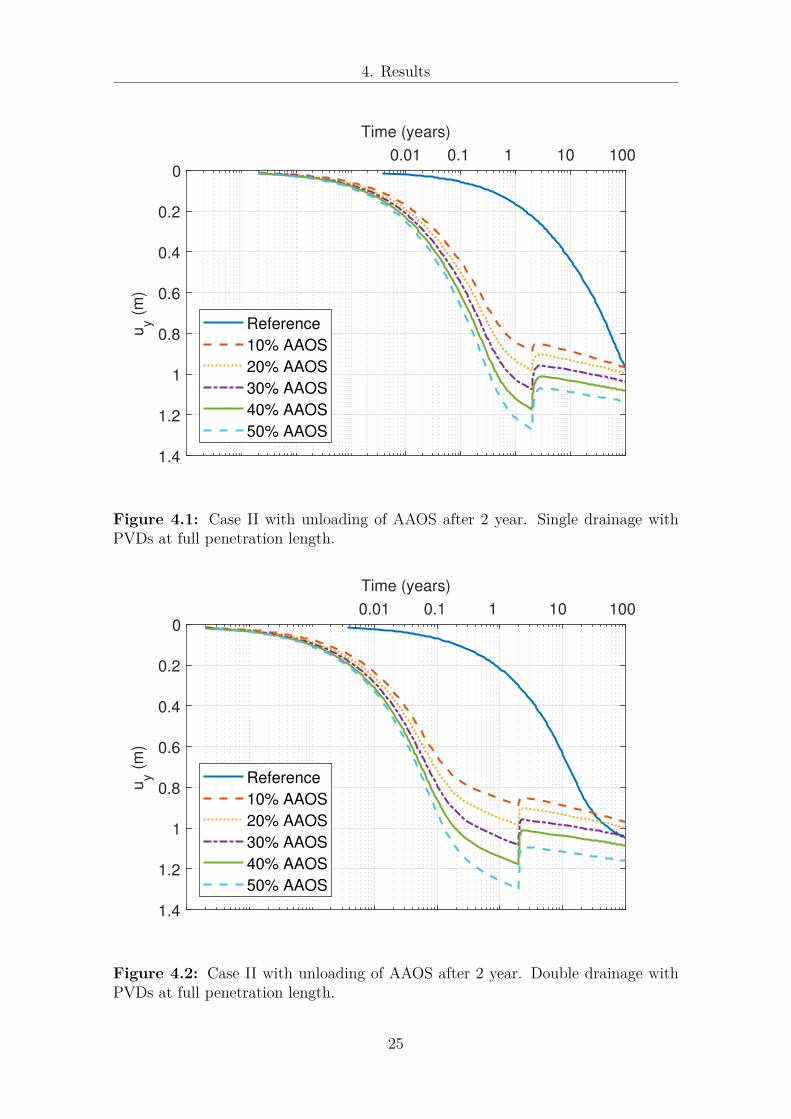
Figure 4.1 and 4.2 illustrates the results for single- and double drainage conditions forthe different surcharge loads. In Geosuite Settlement the surcharge was unloadedafter two years, and the expected swelling phenomena occurred. The referencesimulation for SD shows that the EOP is not reached until 100 years, althoughthat is not the case for the DD condition which reached EOP around 30 years.With ground improvements the single drainage condition reached EOP around 0.8years, and for the double drainage it was reached around 0.2 years. The EOPoccurred approximately four times faster for the double drainage condition comparedto the single drainage condition, which is in line with the theory. The correlationis most probably due to that Geosuite Settlement is based on the one-dimensionalconsolidation theory proposed by Terzaghi (1923). In general the settlements afterEOP are low, between 1-100 years the pure creep settlements was approximately15 cm for DD and 10 cm for SD. The low settlements follows the low creep ratesfrom the simulation results. The low creep rates are in line with Leoni et al. (2008),which stated that higher OCR than 1.3 had negligible creep rates. The figuresalso indicates unreasonably high swelling at higher AAOS. It is important to bearin mind that Geosuite Settlement is based on Hypothesis A where creep does notoccurs simultaneously with the primary consolidation. Models based on HypothesisA will have a significant reduction of the total settlements since the contribution ofcreep will start after EOP.

The creep evaluation for these simulations was performed with out any modificationof the original method presented by Ladd (1971). The results obtained from thecreep evaluation are presented in Figure 4.3. From Figure 4.3, it is evident thatnone of the drainage conditions correlates with Ladd’s mean line. The results fromSD and DD-drainage shows significantly lower creep improvement ratios compared to

24

4. Results

0.01 0.1 1 10 100

Time (years)

0

0.2

0.4

0.6

0.8

1

1.2

1.4

uy (

m)

Reference

10% AAOS

20% AAOS

30% AAOS

40% AAOS

50% AAOS

Figure 4.1: Case II with unloading of AAOS after 2 year. Single drainage withPVDs at full penetration length.

0.01 0.1 1 10 100

Time (years)

0

0.2

0.4

0.6

0.8

1

1.2

1.4

uy (

m)

Reference

10% AAOS

20% AAOS

30% AAOS

40% AAOS

50% AAOS

Figure 4.2: Case II with unloading of AAOS after 2 year. Double drainage withPVDs at full penetration length.

25

4. Results

10 20 30 40 50

AAOS (%)

0

0.2

0.4

0.6

0.8C

'/C

Single drainage

Double drainage

Ladd's mean

Single drainage mean

Double drainage mean

Figure 4.3: Creep improvement ratio due to surcharge, derived from both drainageconditions in case II using the method proposed by Ladd (1971).

Ladd’s mean line. This implies that the creep rates are expected to be lower duringthe embankments life time according to this analysis. Comparing the two drainageconditions, it can be seen that slightly lower creep improvement ratios are expectedfor double drainage condition, although, the results indicates that increasing AAOSwill not necessarily produce lower creep rate. Another reason could be that soilswith an OCR-value equal or higher than 1.3 has negligible creep rates as statedby Leoni et al. (2008), producing low creep improvement ratios.

The analysis from case II in Geosuite Settlement indicated similar results as inCreep-SCLAY1S. The penetration depth of the PVDs (case III) was also optimisedwith 20% AAOS. The results for case III are illustrated in Figure 4.4 and 4.5.Vertical displacements at centre line of the embankment are plotted against thetime for different penetration depths. The results for single drainage conditionspoint outs that penetration depth between L/H=0.3-0.8 has an impact on end ofprimary consolidation, thus the drain length could be reduced by 10% (L/H=0.9).Although, for double drainage the length of the PVDs could be reduced by 20%(L/H=0.8) without affecting end of primary consolidation. These results are in wellaccordance with results presented in Ikhya and Schweiger (2012), where drain lengthcould be reduced by 20% for the double drainage, and 10% for the single drainagecondition.

26

4. Results

0.01 0.1 1 10 100

Time (years)

0

0.2

0.4

0.6

0.8

1

uy (

m)

L/H = 0.3

L/H = 0.4

L/H = 0.5

L/H = 0.6

L/H = 0.7

L/H = 0.8

L/H = 0.9

L/H = 1

Figure 4.4: Optimisation of penetration length of the PVDs for single drainage.

0.01 0.1 1 10 100

Time (years)

0

0.2

0.4

0.6

0.8

1

uy (

m)

L/H = 0.3

L/H = 0.4

L/H = 0.5

L/H = 0.6

L/H = 0.7

L/H = 0.8

L/H = 0.9

L/H = 1

Figure 4.5: Optimisation of penetration length of the PVDs for double drainage.

27

4. Results

4.2 Simulation results from Creep-SCLAY1S

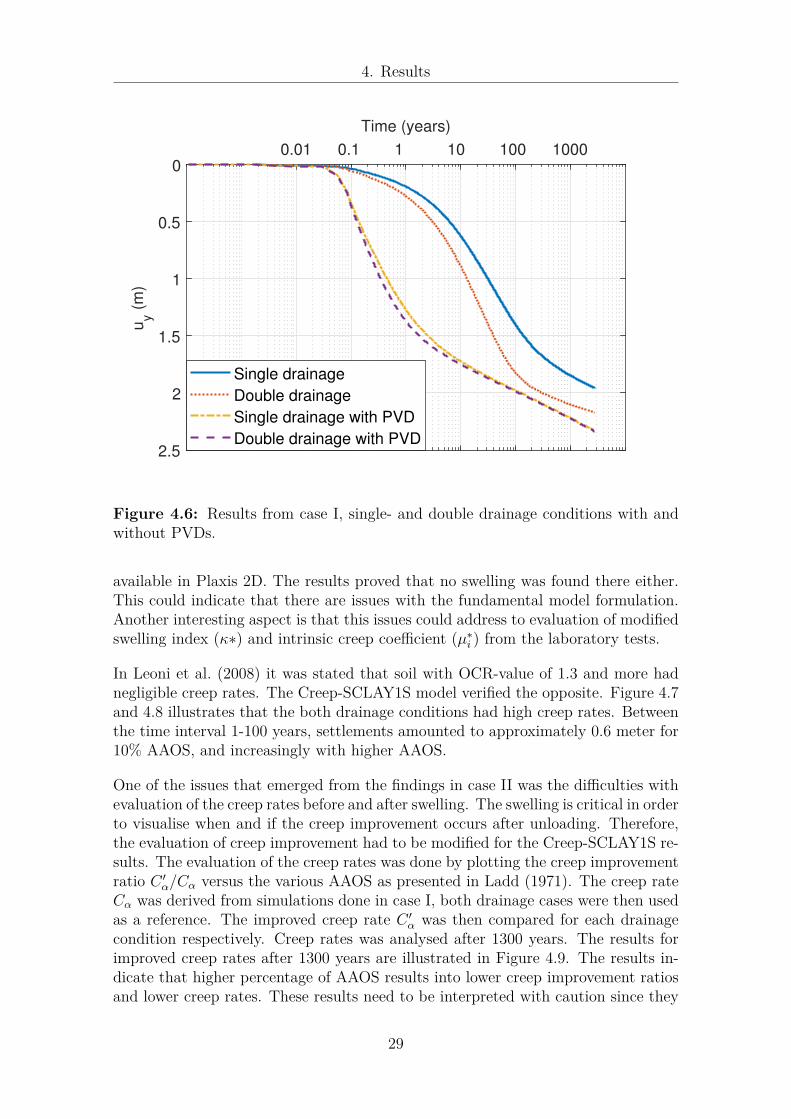
The first simulations were simulated to establish the reference cases for single (SD)-and double drainage (DD) conditions respectively. Case I is presented in Figure 4.6,consisting of single- and double drainage, with and without prefabricated verticaldrains (PVDs). SD and DD without PVDs has an end of primary consolidation(EOP) after approximately 100 and 300 years, respectively. In theory the doubledrainage condition should reach EOP four times faster than the single drainagecondition. In contrast, primary consolidation ends after approximately one yearfor both drainage conditions with PVDs. After 100 years the embankment withPVDs is predicted to settle up to two meters, resulting in equal level as the initialground surface. PVDs significantly improves the EOP and a large share of the totalsettlements has already occurred after one to three years. For the conditions withoutPVDs, large post construction settlements starts to occur after one year. Withoutground improvement that serviceability during the embankments life time (40 years)is most likely affected.

Another interesting aspect is that for the SD condition without PVDs high creeprates are produced. This is suggesting that even after 1000 years primary and sec-ondary consolidation is on-going. In general, better drainage conditions contributesto larger total settlements of the soil. The double drainage condition had a small im-provement on the EOP when PVDs at full depth was activated. The small differencein EOP for the drainage conditions is probably due to the performance of the drains.The change of improved clay layer acting as drains had high enough permeability,which made the drainage condition insignificant. Even in the case without groundimprovements the double drainage conditions did not reach four times faster EOP.This due to that the boundary value problem in this study had different conditionscompared to the ones mentioned earlier in the theory Section 2.1.

Figure 4.7 and 4.8 illustrates the optimisation results of different surcharge loadsfor the SD and DD conditions. The results indicates that a higher percentage ofadjusted amount of surcharge (AAOS) reduces the time for EOP and this becausea higher pore water pressure gradient increase the rate of consolidation. Comparingthe two drainage conditions it was noticed that EOP was occurring earlier for the DDcondition. Analysing the simulations done at 10% AAOS for both types of drainageconditions, it was proven that EOP for SD was reached after approximately threeyears whereas for the DD the EOP ended after approximately one year. Surprisingly,no swelling is predicted after unloading at various AAOS for both conditions. Asingle simulation was performed where the load was left in place for a longer time andwith a higher load than 50% AAOS, still no swelling occurred. This is suggesting thatthe intrinsic creep rates could be higher than any predicted swelling. This could bedue to the Creep-SCLAY1S model does not properly capture the swelling phenomenaafter unloading. Another reason may be that the Creep-SCLAY1S model is basedon Hypothesis B which was mentioned in Section 2.2, producing such extensivesettlements that even a swelling of small magnitude may remain unnoticed. Onesimulation, not presented in these results, was done in the Soft Soil Creep model,

28

4. Results

0.01 0.1 1 10 100 1000

Time (years)

0

0.5

1

1.5

2

2.5

uy (

m)

Single drainage

Double drainage

Single drainage with PVD

Double drainage with PVD

Figure 4.6: Results from case I, single- and double drainage conditions with andwithout PVDs.

available in Plaxis 2D. The results proved that no swelling was found there either.This could indicate that there are issues with the fundamental model formulation.Another interesting aspect is that this issues could address to evaluation of modifiedswelling index (κ∗) and intrinsic creep coefficient (µ∗i ) from the laboratory tests.

In Leoni et al. (2008) it was stated that soil with OCR-value of 1.3 and more hadnegligible creep rates. The Creep-SCLAY1S model verified the opposite. Figure 4.7and 4.8 illustrates that the both drainage conditions had high creep rates. Betweenthe time interval 1-100 years, settlements amounted to approximately 0.6 meter for10% AAOS, and increasingly with higher AAOS.

One of the issues that emerged from the findings in case II was the difficulties withevaluation of the creep rates before and after swelling. The swelling is critical in orderto visualise when and if the creep improvement occurs after unloading. Therefore,the evaluation of creep improvement had to be modified for the Creep-SCLAY1S re-sults. The evaluation of the creep rates was done by plotting the creep improvementratio C ′α/Cα versus the various AAOS as presented in Ladd (1971). The creep rateCα was derived from simulations done in case I, both drainage cases were then usedas a reference. The improved creep rate C ′α was then compared for each drainagecondition respectively. Creep rates was analysed after 1300 years. The results forimproved creep rates after 1300 years are illustrated in Figure 4.9. The results in-dicate that higher percentage of AAOS results into lower creep improvement ratiosand lower creep rates. These results need to be interpreted with caution since they

29

4. Results

0.01 0.1 1 10 100 1000 10000

Time (years)

0

0.5

1

1.5

2

2.5

3

3.5

uy (

m)

Reference

10% AAOS

20% AAOS

30% AAOS

40% AAOS

50% AAOS

Figure 4.7: Case II with unloading of AAOS after 1 year. Single drainage withPVDs at full penetration length.

0.01 0.1 1 10 100 1000 10000

Time (years)

0

0.5

1

1.5

2

2.5

3

3.5

uy (

m)

Reference

10% AAOS

20% AAOS

30% AAOS

40% AAOS

50% AAOS

Figure 4.8: Case II with unloading of AAOS after 1 year. Double drainage withPVDs at full penetration length.

30

4. Results

10 20 30 40 50

AAOS (%)

0

0.2

0.4

0.6

0.8

C'

/C

Single drainage

Double drainage

Ladd's mean

Single drainage mean

Double drainage mean

Figure 4.9: Creep improvement ratio due to surcharge, derived from both drainageconditions in case II after 1300 years.

only occur around 1300 years. Performing the same evaluation for another timeframe would produce different results. However, the results for double drainagecondition supports the procedure presented by Ladd (1971) that mimics the typicalloading regime for embankment constructions. The results for single drainage alsoindicates the expected behaviour, although the reduction of creep rate seems to belower with the incremental of AAOS.

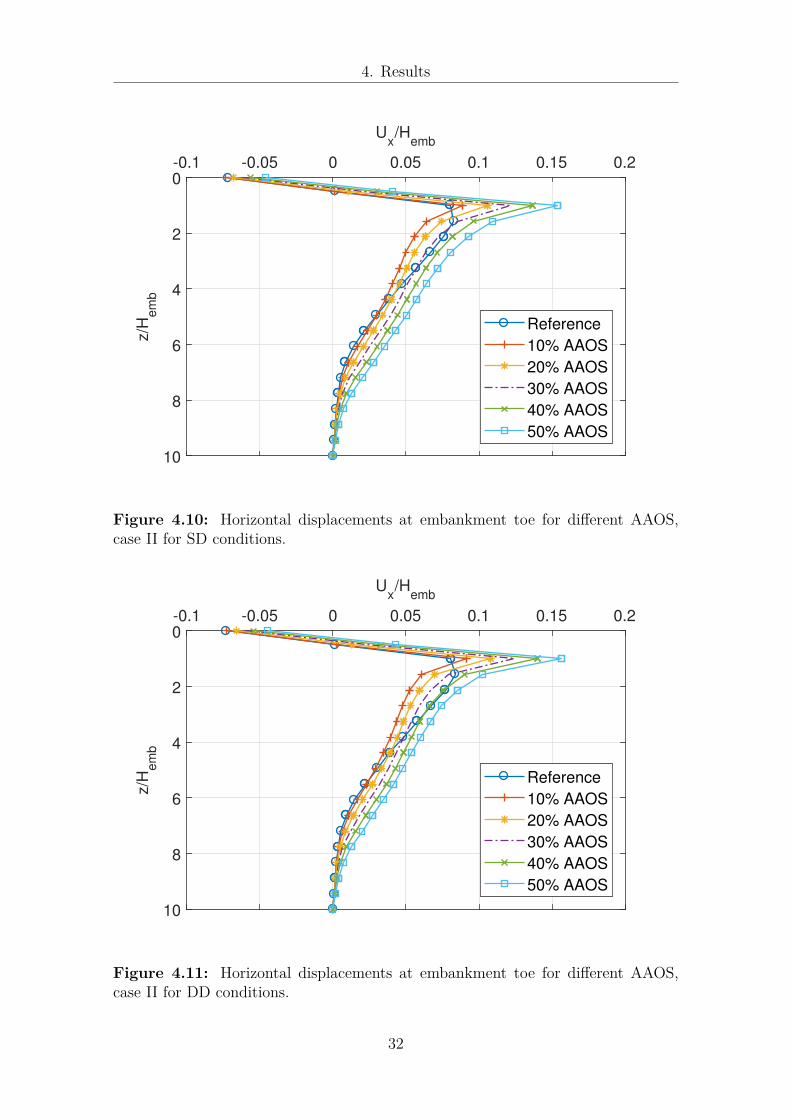
In Figure 4.10 and 4.11 horizontal displacements are presented for both drainageconditions. The figures shows horizontal displacements versus soil depth, and arenormalised with the embankment height. Analysing the both conditions, no sig-nificant difference was noted between the SD and DD-conditions. The horizontaldisplacements was affected by varying magnitude of the AAOS, similar to the re-sults for the vertical displacements. These results suggests that larger horizontaldisplacements occurs at higher AAOS. At 50% AAOS the displacements are highenough to affect up to 30 cm at each side of the embankment. Although, thesedisplacements are fully developed after approximately 2700 years.

After the simulations with different AAOS was finished, the analysis proceeded withthe optimisation of the penetration depth (case III). This case was optimised with thesurcharge load 8 kPa which is equal to 20% AAOS. This surcharge load was chosensince higher loads gave excessively large settlements, lower loads seemed unreason-ably low for a two meter high embankment construction. In Figure 4.12 and 4.13the vertical displacements depth against time are plotted for different penetration

31

4. Results

-0.1 -0.05 0 0.05 0.1 0.15 0.2

Ux/H

emb

0

2

4

6

8

10

z/H

em

b

Reference

10% AAOS

20% AAOS

30% AAOS

40% AAOS

50% AAOS

Figure 4.10: Horizontal displacements at embankment toe for different AAOS,case II for SD conditions.

-0.1 -0.05 0 0.05 0.1 0.15 0.2

Ux/H

emb

0

2

4

6

8

10

z/H

em

b

Reference

10% AAOS

20% AAOS

30% AAOS

40% AAOS

50% AAOS

Figure 4.11: Horizontal displacements at embankment toe for different AAOS,case II for DD conditions.

32

4. Results

0.01 0.1 1 10 100 1000 10000

Time (years)

0

0.5

1

1.5

2

2.5

3

uy (

m)

L/H = 0.3

L/H = 0.4

L/H = 0.5

L/H = 0.6

L/H = 0.7

L/H = 0.8

L/H = 0.9

L/H = 1

Figure 4.12: Optimisation of penetration length for single drainage.

depths. The figures indicate that the penetration depths of 0.3-0.5 for both drainageconditions affects the EOP, resulting in prolonging the time needed for primary con-solidation to end. Further on, the analysis showed that the penetration depth couldbe reduced up to L/H=0.6 without affecting the consolidation process. These resultsare in agreement with those obtained by Indraratna and Rujikiatkamjorn (2008),which concluded that the drain length can be reduced with 40%. The length ofthe PVDs could even be reduced up 50% which slightly influences the consolidationprocess. However, these results is contrary to that of Geng et al. (2011), whereit was concluded that the length of PVDs in general can be reduced with 20% toachieve a normalised settlement of 90%. Ikhya and Schweiger (2012) found that thedrain length for a homogeneous soil could be reduced up to 20% for double drainageand only 10% for single drainage, without significantly affecting the consolidationprocess. These results together provide important insights into how deep the drainsshould be installed at ground improvements.

Figure 4.14 and 4.15 presents the results for horizontal displacements for differentpenetration lengths of the PVDs. In the figures depth of the soil versus the hori-zontal displacements is plotted, and both axes are normalised with the embankmentheight. Analysing the results from the figures no significant difference was noted be-tween the two drainage conditions. Lower penetration depths than 50% shows mostdeviations from the deeper penetration lengths. There was a significant positive cor-relation between the results from this study with Indraratna and Rujikiatkamjorn(2008) considering the lateral displacements. In Indraratna and Rujikiatkamjorn(2008) it can be seen that no distinguishable difference was noticed for the horizon-

33

4. Results

0.01 0.1 1 10 100 1000 10000

Time (years)

0

0.5

1

1.5

2

2.5

3

uy (

m)

L/H = 0.3

L/H = 0.4

L/H = 0.5

L/H = 0.6

L/H = 0.7

L/H = 0.8

L/H = 0.9

L/H = 1

Figure 4.13: Optimisation of penetration length for double drainage.

tal displacements when reduction of the PVDs are in the range L/H=1-0.5. However,the simulations in this study are extended to even lower penetration depths than50%. The lower penetration depths shows a deviating trend, resulting in largerhorizontal displacements between the range z/Hemb = 2− 5.

34

4. Results

-0.05 0 0.05 0.1

Ux/H

emb

0

2

4

6

8

10

z/H

em

b

L/H = 0.3

L/H = 0.4

L/H = 0.5

L/H = 0.6

L/H = 0.7

L/H = 0.8

L/H = 0.9

L/H = 1

Figure 4.14: Horizontal displacements at embankment toe for single drainage whenoptimising penetration length of the PVDs.

-0.05 0 0.05 0.1

Ux/H

emb

0

2

4

6

8

10

z/H

em

b

L/H = 0.3

L/H = 0.4

L/H = 0.5

L/H = 0.6

L/H = 0.7

L/H = 0.8

L/H = 0.9

L/H = 1

Figure 4.15: Horizontal displacements at embankment toe for double drainagewhen optimising penetration length of the PVDs.

35

5Conclusion

The aim of the present research was to examine if creep could be eliminated orreduced with the support of ground improvement. Numerical modelling was assessedto analyse three different cases in Geosuite Settlement and Plaxis 2D. This in orderto find the optimal design of the surcharge load and prefabricated vertical drains.

The study has shown that Geosuite Settlement captures the swelling phenomena.The swelling occurred instantly and for higher loads it amounted up to 10 cm,which seems unreasonable. The evaluation of creep improvement ratio showed thatthe results were not in line with Ladd (1971) proposal of mean line. However,the results from Geosuite Settlement implies that if higher AAOS is applied, thehigher reduction of creep rate after unloading. High magnitude of AAOS should beapplied with caution, since these produce excessive settlements which may affect theconstructions serviceability. The evaluated results for optimisation of penetrationlength shows that the penetration depth could be reduced up to 10% for singledrainage condition without significantly affecting the consolidation process. On theother hand, for the double drainage condition, penetration depth could be reducedby 20% without significantly affecting EOP.

This study has also identified that Creep-SCLAY1S does not capture the swellingphenomena properly. In general, the model predicts excessive settlements, wheresecondary compression amounts up to approximately 30 percent of the total settle-ments. From the optimisation results, it can be concluded that increasing AAOS willnot necessarily improve the creep rates, although, after 1300 years it is evident thatcreep rates was significantly improved by higher AAOS. Even here caution should betaken regarding the high surcharge loads contributing to excessive settlements. Theoptimisation results also proves that the penetration length of the prefabricated ver-tical drains could be reduced up to 40% without affecting the consolidation process,which is valid for the single and double drainage conditions.

A limitation of this study is that no swelling was noted in the Creep-SCLAY1Ssimulations. Therefore, the method proposed by Ladd (1971) had to be modified.Even when the modification was done, the results indicated that creep rates couldnot be improved within the scope of practical applications. Results from GeosuiteSettlement enabled using the method proposed by Ladd (1971) and it could beconcluded that creep could not be eliminated, although significant reduced creep

36

5. Conclusion

rates was achieved.

Further work should focus on investigating the model formulations for the Soft SoilCreep and Creep-SCLAY1S models. The works should look into the the swellingwhich has passed unnoticed in this study. One suggested approach is to perform asensitivity analysis of the modified swelling index (κ∗) and intrinsic creep coefficient(λ∗i). Additionally, if a similar study is made, embankments with available long-term field measurements should be included in the analysis.

37

Bibliography

Alm, L.-O. (2000). Course Compendium, Road and Street Design.

Almeida, M. and Marques, E. (2013). Design and Performance of Embankments onVery Soft Soils. CRC Press.

Alén, C. (1998). On probability in geotechnics. PhD thesis, Chalmers University ofTechnology.

Amavasai, A. (2016). Parameter derivation and its validation for creep-sclay1s modelfrom utby samples. Technical report, Deparment of Geotechnical Engineering ofChalmers Technical University, Gothenburg.

Balasubramaniam, A. S., Cai, H., Zhu, D., Surarak, C., and Oh, E. Y. N. (2010).Settlements of embankments in soft soils. Geotechnical Engineering Journal ofthe SEAGS & AGSSEA.

Brand, E. W. and Brenner, R. P. (1981). Soft Clay Engineering. ELSEVIER SCI-ENTIFIC PUBLISHING COMPANY.

Chai, J.-C., Shen, S.-L., Miura, N., and Bergado, D. T. (2001). Simple method ofmodeling pvd-improved subsoil. Journal of Geotechnical and GeoenvironmentalEngineering, 127.

Claesson, P. (2003). Long term settlements in soft clays. PhD thesis, ChalmersUniversity of Technology.

Conroy, T., Fahey, D., Buggy, F., and Long, M. (2015). Control of secondary creepin soft alluvium soil using surcharge loading. Technical report, University CollegeDublin.

Fatahi, B., Lê, M., and Khabbaz, H. (2013). Soil creep effects on ground lateraldeformation and pore water pressure under embankments. Geomechanics andGeoengineering. DOI: 10.1080/17486025.2012.727037.

Geng, X., Indraratna, B., and Rujikiatkamjorn, C. (2011). Effectiveness of partiallypenetrating vertical drains under a combined surcharge and vacuum preloading.Canadian Geotechnical Journal, 48(6):970–983.

Gras, J.-P., Sivasithamparam, N., Karstrunen, M., and Dijkstra, J. (2015). Permis-

38

Bibliography

sible range of model parameters for natural fine-grained materials. Acta Geotech-nica. DOI: 10.1007/s11440-017-0553-1.

Grimstad, G., Degago, A. S., Nordal, S., and Karstunen, M. (2010). Modelingcreep and rate effects in structured anisotropic soft clays. Acta Geotechnica. DOI:10.1007/s11440-010-0119-y.

Hansbo, S. (1981). Consolidation of fine-grained soils by prefabricated drains. InProceedings of the 10th International Conference on Soil Mechanics and Founda-tion Engineering, Stockholm, Edited by Publications Committee of the ICSMFE.A.A. Balkema, Rotterdam, The Netherlands, 3:677–682.

Ikhya, I. and Schweiger, H. (2012). Numerical modelling of floating prefabricatedvertical drains in layered soil. Acta Geotechnica Slovenica.

Indraratna, B. and Rujikiatkamjorn, C. (2008). Effects of partially penetratingprefabricated vertical drains and loading patterns on vacuum. University of Wol-longong. http://dx.doi.org/10.1061/40971(310)74.

Kalmykova, Y., Rosado, L., and Patrício, J. (2015). Resource consumption driversand pathways to reduction: economy, policy and lifestyle impact on materialflows at the national and urban scale. Journal of Cleaner Production, pages 1–11.http://dx.doi.org/10.1016/j.jclepro.2015.02.027.

Karlsson, M., Emdal, A., and Dijkstra, J. (2016). Consequences of sample distur-bance when predicting long-term settlements in soft clay. Chalmers University ofTechnoligy.

Karstunen, M., Sivasithamparam, N., Bringreve, R., and Bonnier, P. (2013). Mod-elling rate-dependent behaviour of structured clays. In International Conferenceon Installation Effects in Geotechnical Engineering (ICIEGE), pages 43–50.

Kirsch, K. and Bell, A. (2013). Ground Improvement. Spon Press.

Knappett, J. and Craig, R. (2012). Craig’s Soil Mechanics. Spon Press, 8 edition.

Ladd, C. C. (1971). Settlement analyses of cohesive soils. Technical report, Depart-ment of Civil Engineering, M.I.T., Canbridge, Massachusetts.

Ladd, C. C., Foott, R., Ishihara, K., Schlosser, K., and Poulos, H. G. (1977). Stress-deformation and strength characteristics. state-of-the-art report. Géotechnique,page 421–494. DOI 10.1680/geot.2001.51.10.859.

Leoni, M., Karstunen, M., and Vermer, P. (2008). Anisotropic creep model for softsoils. Geotechnique, 58:215–226. http://dx.doi.org/10.1680/geot.2008.58.3.215.

Mehner, H. (2017). Urban development in gothenburg. http://goo.gl/Lm8mF3.

Mesri, G. and Funk, J. R. (2015). Settlement of the kansai international airportislands. Journal of Geotechnical and Geoenvironmental Engineering, 14. http://dx.doi.org/10.1061/(ASCE)GT.1943-5606.0001224#sthash.uPpp9Lfr.dpuf.

39

Bibliography

Mitchell, J. K. and Soga, K. (2005). Fundamentals of Soil Behavior. John Wiley &Sons, Inc., Hoboken, New Jersey, 3 edition.

Navarro, V. and Alonso, E. E. (2001). Secondary compression of clays as a local de-hydration process. Géotechnique, page 859–869. DOI 10.1680/geot.2001.51.10.859.

Puzrin, Alonso, and Pinyol (2010). Geomechanics of Failures. Springer Netherlands.

Sivasithamparam, N., Karstrunen, M., and Bonnier, P. (2015). Modelling creepbehaviour of anisotropic soft soils. Computers and Geotechnics 69, 3:1–12.http://dx.doi.org/10.1016/j.compgeo.2015.04.015.

Swedish Standard Institute, S. (1991). Geotekniska provningsmetoder – kompres-sionsegenskaper – Ödometerförsök. crs-försök – kohesionsjord. Geoteknik ochgeokonstruktioner, SIS/TK 183.

Swillingand, M. and Robinson, B. (2013). Urban resource flows and the governanceof infrastructure transitions. Environmental Development, pages 152–153. http://dx.doi.org/10.1016/j.envdev.2013.09.002.

Terzaghi, K. (1923). Die Berechung der Durchlässigkeitsziffer des Tones aus demVerlauf der hydrodynamishe Spannungserscheinungen., volume 132. John Wileyand Sons, Inc.

Terzaghi, K. (1943). Theoretical Soil Mechanics. John Wiley and Sons, Inc.

Tewatia, S. K., Bose, P. R., Sridharan, A., and Rath, S. (2007). Stress induced timedependent behavior of clayey soils. Geotechnical and Geological Engineering, page239–255. DOI 10.1007/s10706-006-9107-2.

Wheeler, S. J., Näätänen, A., Karstunen, M., and Lojander, M. (2003). Ananisotropic elastoplastic model for soft clays. Canadian Geotechnical Journal,pages 403–418.

40

AAppendix

A.1 Derivation of improved permeability (keq)

Table A.1: Calculation of improved permeability to represent the PVDs in thesoil.

Parameters value Unitcv 3.15 m2/yrch 4.0 m2/yrt t yrkh 1× 10−9 m/sks 2.5× 10−10 m/sds 0.53 mdw 0.07 mUv,h 0.9 %Tv 0.03 −Uv 0.27 %Ur 0.88 %s 8 −S 2 mD 2.26 mTr 0.2 −n 34.18 −µ 9.02 −Ur 0.16 −qw 4.8× 10−6 m3/skev 1.4× 10−6 m/skev 1.4× 10−2 m/day

I

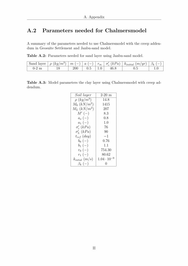
A. Appendix

A.2 Parameters needed for Chalmersmodel

A summary of the parameters needed to use Chalmersmodel with the creep adden-dum in Geosuite Settlement and Janbu-sand model.

Table A.2: Parameters needed for sand layer using Janbu-sand model.

Sand layer ρ (kg/m3) m (−) a (−) rm σ′c (kPa) kinitial (m/yr) βk (−)0-2 m 18 200 0.5 1.0 46.8 0.5 1.0

Table A.3: Model parameters the clay layer using Chalmersmodel with creep ad-dendum.

Soil layer 2-20 mρ (kg/m3) 14.8M0 (kN/m2) 1415ML (kN/m2) 207M ′ (−) 8.3ao (−) 0.8a1 (−) 1.0σ′c (kPa) 76σ′L (kPa) 90tref (day) −1b0 (−) 0.76b1 (−) 1.1r0 (−) 754.30r1 (−) 80.62

kintial (m/s) 1.04 · 10−9

βk (−) 0

II

A. Appendix

A.3 Denotation of creep number, r

Below, equation for denoting the creep addendum parameters are presented.

r1 = 75w1.5N

(A.1)

where wN is the natural water content in the soil.

r0 = ψ · (b1 − b0) + r1 (A.2)

where the constant ψ determines the rate of creep. Usually, the constant ψ is setbetween 2000-3000. If large creep rate is desired low values are set and vice verse.

b0 = σ′0σ′c

(A.3)

In table A.4, the calculated creep addendum parameters for Chalmersmodel arepresented.

Table A.4: Calculated parameters for Chalmersmodel with creep addendum.

Term Unit Clay layerr1 − 80.62ψ − 2000wN % 95.3r0 − 754.30b0 − 0.76b1 − 1.1σ′0 kN/m2 58σ′c kN/m2 76

III

A. Appendix

A.4 Parameters needed for Creep-SCLAY1S

In the following tables, parameters used to simulate the boundary value problemwith Creep-SCLAY1S model are presented and derived by Amavasai (2016).

The additional initial stress state parameters for the soil layers.

Table A.5: The additional initial stress state parameters for the soil layers.

Material Model ρ E v K0 ϕ′ c′

(−) (−) (kg/m3) (MPa) (−) (−) (◦) (kPa)Embankment MC 2.0 25 0.3 1 35 2

Sand MC 1.8 5 0.3 0.5 30 5Dry crust MC 1.8 7 0.3 0.7 30 1

Clay Creep-SCLAY1S 1.55 1 1 1 30 N/A

Table A.6: Isotropic parameters used for the clay layer.

Isotropic parameters κ∗ λ∗i υ Mc Me ϕ′

(−) (−) (−) (−) (−) (−) (◦)Clay 0.01 0.122 0.18 1.075 0.79 30

Table A.7: Anisotropic parameters used for the clay layer.

Anisotropic parameters α0 ω ωd(−) (−) (−) (−)Clay 0.4125 30 0.6067

Table A.8: Destructuration parameters used for the clay layer.

Destructuration parameters χ0 ξ ξd(−) (−) (−) (−)Clay 5.08 9 0.2

Table A.9: Viscous parameters used for the clay layer.

V iscous parameters µ∗i τ(−) (−) (days)Clay 0.0013 1

IV