numerical modeling and analysis of composite beam structures
TRANSCRIPT

Numerical Modeling and Analysis of Composite Beam
Structures Subjected to Torsional Loading
Kunlin Hsieh
Thesis submitted to the faculty of the Virginia Polytechnic Institute and State University
in partial fulfillment of the requirements for the degree of
Master of Science in
Engineering Mechanics
John C. Duke (Chair) Raymond H. Plaut
Scott W. Case
May 3, 2007 Blacksburg, Virginia
Keywords: Homogenization, Volume Fraction, Laminated Composites, Torsional Rigidity
Copyright ©2007, Kun-Lin Hsieh

Numerical Modeling and Analysis of Composite Beam Structures Subjected to Torsional Loading
Kunlin Hsieh
ABSTRACT
Torsion of cylindrical shafts has long been a basic subject in the classical theory of elasticity.
In 1998 Swanson proposed a theoretical solution for the torsion problem of laminated
composites. He adopted the traditional formulation of the torsion problem based on Saint
Venant’s torsion theory. The eigenfunction expansion method was employed to solve the
formulated problem. The analytical method is proposed in this study enabling one to solve the
torsion problem of laminated composite beams. Instead of following the classical Saint Venant
theory formulation, the notion of effective elastic constant is utilized. This approach uses the
concept of elastic constants, and in this context the three-dimensional non-homogeneous
orthotropic laminate is replaced by an equivalent homogeneous orthotropic material. By adopting
the assumptions of constant stress and constant strain, the effective shear moduli of the
composite laminates are then derived. Upon obtaining the shear moduli of the equivalent
homogeneous material, the effective torsional rigidity of the laminated composite rods can be
determined by employing the theory developed by Lekhnitskii in 1963. Finally, the predicted
results based on the present analytical approach are compared with those by the finite element,
the finite difference method and Swanson’s results.

iii
Acknowledgements
I would like to sincerely thank my committee chair and advisor Dr. John C. Duke for his
generosity, patience, and guidance throughout this thesis and my graduation program. His
thoughtfulness and willingness to help are deeply appreciated. It has been a pleasure to have him
as an advisor. My gratitude and appreciation also go to Dr. Raymond H. Plaut and Dr. Scott W.
Case for serving as members of my committee.
I would like to thank my friend Mr. Haekyu Hur for taking time with me to discuss my
research problem. Your long-term support and encouragement are truly appreciated.
Most importantly, I would like to thank my parents, Mr. Joneming Hsieh and Mrs. Wei Jui,
my older sister Huiya Hsieh, and my younger sister Menghua Hsieh for their love, support, and
encouragement throughout my entire graduate study. This work is dedicated to all of you.
iv
Table of Contents .
Abstract……………………………………………………………………………………………ii
Acknowledgements………………………………………………………………………………iii
List of Figures…………………………………………………………………………………….vi
List of Tables…………………………………………………………………………………….vii
Chapter 1: Introduction and Literature Review…………………………………………………...1
1.1 Introduction…………………………………………………………………………….1
1.2 Literature Review………………………………………………………………………3
1.2.1 Torsion of Circular Cross Section……………………………………………..3
1.2.2 Torsion of Non-Circular Cross Section……………………………………….4
1.2.3 Solutions using Prandtl’s Stress Function…………………………………….7
1.2.4 Analytical Solutions for Rectangular Cross Section…………………………..9
Chapter 2: Effective Elastic Constants for Laminated Composite………………………………11
2.1 Introduction…………………………………………………………………………..11
2.2 Theoretical Background……………………………………………………………...13
2.3 Hooke’s Law for Monoclinic Materials……………………………………………...14
2.4 Effective Constants…………………………………………………………………..18
2.5 Verification Examples……………………………………………………………….27
Chapter 3: Torsional Response of Laminated Composite Beam………………………………...32
3.1 Introduction…………………………………………………………………………..32
3.2 General Formulation…………………………………………………………………33
3.3 Formulation for Orthotropic Composite Beams………………………………..……35
3.4 Analytical Model for Rectangular Laminated Composites…………..……………...37
Chapter 4: Finite Element Analysis……………………………………………………………...45
4.1 Introduction…………………………………………………………………………..45
4.2 Finite Element Procedure…………………………………………………………….52
v
4.3 Verification Examples……………………………………………………………….53
Chapter 5: Finite Difference Method…………………………………………………………….69
5.1 Introduction…………………………………………………………………………..69
5.2 Finite Difference Equations…..……………………………………………………...70
5.3 Verification Examples……………………………………………………………….77
Chapter 6: Results and Comparisons…………………………………………………………….84
6.1 Material Properties…………………………………………………………………...84
6.2 Analysis Models……………………………………………………………………...87
6.2.1 Convergence Study…………………………………………………………….88
6.2.2 Results and Comparisons………………………………………………………96
Chapter 7: Summary and Conclusions...………………………………………………………..100
References………………………………………………………………………………………102
Vita……………………………………………………………………………………………...105

vi
List of Figures
Figure 1.1: Circular Prismatic Bar under Torsional Loading……………………………………4
Figure 1.2: Elliptical Cross Section……………………………………………………………...8
Figure 1.3: Equilateral Triangle Cross Section…………………………………………………..8
Figure 1.4: Rectangular Cross Section…………………………………………………………...9
Figure 2.1: The Representative Element for Monoclinic Materials……………………………14
Figure 2.2: The Representative Element of Layered Medium………………………………….19
Figure 3.1: General Cross Section Composed of Orthotropic Media…………………………..34
Figure 3.2: Cross Section of Laminated Composites…………………………………………...39
Figure 4.1: 2D Rectangular Beam Cross Section……………………………………………....49
Figure 4.2: PLANE77 Geometry……………………………………………………………….53
Figure 4.3: Rectangular Cross Section………………………………………………………….54
Figure 4.4: Rectangular Cross Section Composed of Two Different Materials………………..57
Figure 4.5: Cross Section of Orthogonal Beam………………………………………………...64
Figure 5.1: Finite Difference Approximation of Function )(xg ……………………………….71
Figure 5.2: Rectangular Mesh…………………………………………………………………..74
Figure 5.3: Finite Difference Grids……………………………………………………………..76
Figure 6.1: Transformation Relations between 1-2-3 and x-y-z Coordinate Systems………….86
Figure 6.2: The Analysis Model………………………………………………………………..87
Figure 6.3: Convergence Study for Finite Element Method…………………………………....89
Figure 6.4: Convergence Study for Finite Difference Method………………………………....90
Figure 6.5: Contour Plot for Prandtl’s Stress Function
(Graphite-polymer Laminates s]0/15[ )…………………………………………….91
Figure 6.6: Mesh Plot for Analysis Model (element size = 0.8 mm)…………………………..92
Figure 6.7: Mesh Plot for Analysis Model (element size = 0.5 mm)…………………………..93
Figure 6.8: Mesh Plot for Analysis Model (element size = 0.25 mm)………………………..94
Figure 6.9: Mesh Plot for Analysis Model (element size = 0.2 mm)…………………………95

vii
List of Tables
Table 2.1: Direction Cosine Table……………………………………………………………...15
Table 2.2: Material Properties of Laminas in the Sublaminate……………………………...…28
Table 2.3: Comparison of Effective Moduli for Boron/Epoxy Angle-Plied Laminates……..…29
Table 2.4: Comparison of Effective Moduli for Hybrid Laminates…………………………....31
Table 4.1: Analogy between Torsion Problem and Heat Transfer Problem…………………....51
Table 4.2: Comparison of 1k Value between Analytical and ANSYS Results…………….…...54
Table 4.3: Comparison of 2k Value between Analytical and ANSYS Results……………...….56
Table 4.4: Comparison of Torsional Rigidity between Analytical and ANSYS Solutions
with the Change of Ratio of Shear Moduli 21 / GG ……............................................60
Table 4.5: Comparison of Torsional Rigidity between Analytical and ANSYS Solutions
with the Change of Ratio of Shear Moduli ba /1 ………...……………………...….61
Table 4.6: Comparison of Torsional Rigidity between Analytical and ANSYS Solutions
with the Change of Ratio of Shear Moduli ba /2 …………...……………...……….62
Table 4.7: Comparison of β Value between Analytical and ANSYS Results…........................67
Table 4.8: Comparison of 3k Value between Analytical and ANSYS Results………………....67
Table 4.9: Comparison of 4k Value between Analytical and ANSYS Results…………………68
Table 5.1: Comparison of 1k Value between Analytical and FDM Results…………………….77
Table 5.2: Comparison of 2k Value between Analytical and FDM Results……………………77
Table 5.3: Comparison of Torsional Rigidity between Analytical and FDM Solutions
with the Change of Ratio of Shear Moduli 21 / GG ……………...………………….78
Table 5.4: Comparison of Torsional Rigidity between Analytical and FDM Solutions
with the Change of Ratio of Shear Moduli ba /1 ………………...…………………79
Table 5.5: Comparison of Torsional Rigidity between Analytical and FDM Solutions
with the Change of Ratio of Shear Moduli ba /2 …………………………………...80
Table 5.6: Comparison of β Value between Analytical and FDM Results…………………….81

viii
Table 5.7: Comparison of 3k Value between Analytical and FDM Results……………………82
Table 5.8: Comparison of 4k Value between Analytical and FDM Results……………………83
Table 6.1: Material Properties of Graphite-polymer Composite…………………………….…84
Table 6.2: Material Properties of Glass-polymer Composite…………………………………..85
Table 6.3: Shear Moduli for Different Ply-angles (Graphite-polymer Composite)…………....85
Table 6.4: Shear Moduli for Different Ply-angles (Glass-polymer Composite)……………….85
Table 6.5: Convergence Study for Finite Element Method…………………………………….88
Table 6.6: Convergence Study for Finite Difference Method………………………………….89
Table 6.7: Comparisons of Torsional Rigidity between Present Analytical Method
and ANSYS Results (Graphite-polymer Composite)……………………….………97
Table 6.8: Comparisons of Torsional Rigidity between Present Analytical Method
and ANSYS Results (Glass-polymer Composite)……………………….………....98

1
Chapter 1 Introduction and Literature Review 1.1 Introduction
Composite materials have been widely used to improve the performance of various types of
structures. Compared to conventional materials, the main advantages of composites are their
superior stiffness to mass ratio as well as high strength to weight ratio. Because of these
advantages, composites have been increasingly incorporated in structural components in various
industrial fields. Some examples are helicopter rotor blades, aircraft wings in aerospace
engineering, and bridge structures in civil engineering applications.
Torsion of cylindrical shafts has long been a basic subject in the classical theory of elasticity
(Timoshenko and Goodier, 1970). The stiffness of a cylindrical shaft under torsional loading is
often of interest in the study of torsion problems. The axial displacement field of the cross-
section is assumed to not vary along the axial direction away from the ends of the shaft. Under
this assumption, the torsional rigidity is only dependent on the shape of the cross-section. The
governing equations of this boundary value problem can be formulated in terms of a Laplace or
Poisson Equation. Within the former one, one uses the warping function as a dependent variable,
while in the latter the Prandtl’s stress function is used. The solutions for the warping and
Prandtl’s stress function have been obtained exactly for simple cross-sectional shapes such as a
circle, annulus, ellipse, rectangle, and triangle. For more complicated shapes, numerical methods
are usually employed, such as, for example, the finite difference method (Ely and Zienkiewicz,
1960), finite element method (Herrmann, 1965; Karayannis, 1995; Li at al., 2000), and boundary
element method (Jawson and Ponter, 1963; Friedman and Kosmatka, 2000; Sapountzakis, 2001;
Sapountzakis and Mokos, 2001, 2003). Some authors use the approach of combination of
experimental and analytical methods to predict the effective in-plane and out-of-plane shear
moduli of structural composite laminates (Davalos, 2002).
Due to the extensive use of composite materials, the study of compound bars under torsion
becomes a very important topic. Compared to homogeneous cylindrical shafts, the torsional
behavior of composite shafts is considerably more complicated. The torsional rigidity not only
depends on the global cross-sectional geometry, but also on the properties and configurations of
each constituent. The analytical solution of compound bars under torsion was first obtained by
Muskhelishvili (1963), where the solution was expressed in terms of eigenfunctions. Packham

2
and Shail (1978) used linear combinations of solutions of a homogeneous shaft to solve the
problem in which the cross section is symmetric with respect to the common boundary.
The elastic properties of non-homogeneous anisotropic beams are usually of engineering
interest. Torsional rigidities of multilayered composite beams are especially needed when
structures are under torsional loading. Savoia and Tullini (1993) analyzed the torsional response
of composite beams of arbitrary cross section. The boundary value problem was formulated in
terms of both warping and Prandtl’s stress function. Using the eigenfunction expansion method,
the exact solution of rectangular multilayered orthotropic beams under uniform torsion was
derived. Swanson (1998) extended the existing solutions of torsion of orthotropic laminated
rectangular beams to the high aspect ratio case. Based on the membrane analogy, an approximate
solution of general, thin, laminated, open cross sections was derived.
In this study, one analytical approach will be proposed to solve the torsion problem of
laminated composite beams that consist of orthotropic sublaminates. The present approach uses
the concept of elastic constants (Chou, et al., 1972), in which the three-dimensional non-
homogeneous orthotropic laminate is replaced by an equivalent homogeneous orthotropic
material. By considering a small element consisting of n layers from the composite material, this
small element is assumed to represent the behavior of the overall composite laminate. We will
consider that this element is under a uniform state of stress when the composite laminate is under
arbitrary loading. Two assumptions have to be implemented: first, the normal strains and shear
strains parallel to the plane of layers are uniform and the same for each constituent and the
corresponding stresses are averaged. Second, the normal stresses and shear stresses
perpendicular to the plane of layers are uniform and equal for each constituent and the
corresponding strains are averaged. Under these two assumptions, the equilibrium at each sub-
laminate interface and compatibility conditions of materials are satisfied automatically. As the
thickness of each layer approaches zero, the overall effective elastic constants are developed.
The effective shear moduli of the composite laminates are used to calculate the overall torsional
rigidity of the orthotropic laminated shaft.

3
1.2 Literature Review
1.2.1 Torsion of Circular Cross Section
Figure 1.1 shows a prismatic bar under torsional loading (Sadda, 1993). The prismatic bar
with radius r is fixed at one end (x-y plane) and subjected to a torque T at the other end. Based
on three assumptions, the torsional response of the circular cross-sectional beam can be derived.
The three assumptions are stated as follows:
(1) The plane normal to the OZ axis remains plane after deformation.
(2) The rotation angle of each cross section is proportional to the distance from the fixed
end (z=0).
(3) The twist angle of each cross section is assumed to be small, so the torsion problem can
be treated as a linear elasticity problem.
Satisfying the equations of equilibrium and boundary conditions, the explicit expressions
of twisting moment and torsional rigidity can be derived. Saint-Venant’s principle states that the
solutions are excellent as long as the plane of solutions is one or two diameters away from the
plane of torque application. The torsional rigidity of an isotropic, circular cross section rod is
defined by the applied torque divided by the twist angle per unit length.
θTGJ = (1.1)
where
=G Shear modulus
== 24rJ π Polar moment of inertia (r = radius of circular cross section)
=T Applied torque
=θ Angle of twist per unit length

4
Figure 1.1 Circular Prismatic Bar under Torsional Loading
1.2.2 Torsion of Non-Circular Cross Section
For a non-circular bar, the torsion problem is solved by the semi-inverse method, which
was developed by Saint-Venant. To use this method, the following two assumptions have to be
made:
(1) The angle of twist of each cross section is proportional to the distance from the fixed
end without any inplane distortion.
(2) All the cross sections will warp in the same way, which means the warping function is
the function of the in-plane coordinates (x, y) only, and independent of the longitudinal
coordinate (z).
The torsion problem of non-circular prismatic bars can be formulated by two approaches.
The first approach is using the warping function, and the second one uses the stress function. The
governing equation, i.e., Laplace’s equation, and associated equations of the torsion problem by
using warping function are displayed below:
X
Y
Z T
O

5
02
2
2
22 =
∂∂+
∂∂=∇
yxψψψ on beam cross section (1.2)
0)()( =+∂∂−−
∂∂
dsdxxyds
dyyxψψ on the boundary surface (1.3)
∫∫ ∂∂−
∂∂++=
R
dxdyxyyxyxGT )( 22 ψψθ (1.4)
∫∫ ∂∂−
∂∂++==
R
dxdyxyyxyxGTGJ )( 22 ψψθ
(1.5)
where
=ψ Warping function
x, y = Coordinates in the cross section
s = Arc length along the bar
=T Applied torque
=G Shear modulus of the prismatic bar
=R Beam cross section
=GJ Torsional rigidity
=θ Angle of twist per unit length
By employing the relations between the warping function and Prandtl’s stress function, the
torsion problem of non-circular cross section can be formulated by the stress function approach.
The relations are shown below:
)( yxGy −∂∂=
∂∂ ψθφ (1.6)
)( xyGx +∂∂−=
∂∂ ψθφ (1.7)
where
6
=φ Prandtl’s stress function
=ψ Warping function
=G Shear modulus of the prismatic bar
=θ Angle of twist per unit length
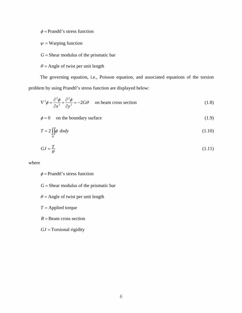
The governing equation, i.e., Poisson equation, and associated equations of the torsion
problem by using Prandtl’s stress function are displayed below:
θφφφ Gyx
22
2
2
22 −=
∂∂+
∂∂=∇ on beam cross section (1.8)
0=φ on the boundary surface (1.9)
∫∫=R
dxdyT φ2 (1.10)
θTGJ = (1.11)
where
=φ Prandtl’s stress function
=G Shear modulus of the prismatic bar
=θ Angle of twist per unit length
=T Applied torque
=R Beam cross section
=GJ Torsional rigidity
7
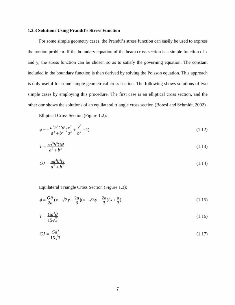
1.2.3 Solutions Using Prandtl’s Stress Function
For some simple geometry cases, the Prandtl’s stress function can easily be used to express
the torsion problem. If the boundary equation of the beam cross section is a simple function of x
and y, the stress function can be chosen so as to satisfy the governing equation. The constant
included in the boundary function is then derived by solving the Poisson equation. This approach
is only useful for some simple geometrical cross section. The following shows solutions of two
simple cases by employing this procedure. The first case is an elliptical cross section, and the
other one shows the solutions of an equilateral triangle cross section (Boresi and Schmidt, 2002).
Elliptical Cross Section (Figure 1.2):
)1( 2
2
2
2
22
22−+
+−=
by
ax
baGba θφ (1.12)
22
33
baGbaT
+= θπ (1.13)
22
33
baGbaGJ
+= π (1.14)
Equilateral Triangle Cross Section (Figure 1.3):
)3)(323)(3
23(2axayxayxa
G +−+−−= θφ (1.15)
315
4θGaT = (1.16)
315
4GaGJ = (1.17)

8
Figure 1.2 Elliptical Cross Section
Figure 1.3 Equilateral Triangle Cross Section
Y
X
b
b
aa
3aY
X
32a

9
1.2.4 Analytical Solutions for Rectangular Cross Section
Figure 1.4 Rectangular Cross Section
The analytical solutions of rectangular cross section beams can be derived by employing
membrane analogy and Fourier series for both isotropic (Boresi and Schmidt, 2002) and
orthotropic (Lekhnitskii, 1981) cases. For the isotropic case, the governing equation, boundary
conditions, and solutions can be expressed as:
Governing Equation:
θφ Gyx 2),(2 −=∇ over the cross section (1.18)
Boundary Conditions:
0),( =± yaφ and 0),( =±bxφ (1.19)
Torsional Rigidity:
]2tanh1)(1921[3)2()2(
,...5,3,155
3
∑∞
=
−=k a
bkkb
abaGGJ ππ
(1.20)
Y
X
a a
b
b

10
For the orthotropic case, the governing equation, boundary conditions, and analytical
solution can be expressed as:
Governing Equation:
θφφ 2),(1),(12
2
2
2
−=∂
∂+∂
∂y
yxGx
yxG zxzy
(1.21)
Boundary Conditions:
0),( =± yaφ and 0),( =±bxφ (1.22)
Torsional Rigidity:
])2
tanh(11921[3
16,...5,3,1
55
3
∑∞
=
−=k zy
zx
zx
zyzy G
Ga
kbkG
GbaGbaGJ π
π (1.23)

11
Chapter 2 Effective Elastic Constants for Laminated Composite
2.1 Introduction
The overall elastic constants for composite materials are of interest in both the academic and
industry field. For thin laminated composites, classical plate theory is employed to analyze the
behavior. To solve the thick laminate problem, high order theory provides adequate accuracy.
The shortages of this theory are that it usually involves more mathematical derivations and is
only suitable for 2-dimensional behavior predictions. Hashin and Shtrikman (1963) proposed
upper and lower bounds for arbitrary geometrical composites. For layered composite materials,
many papers have displayed formulas for elastic moduli.
Three approaches are employed to solve the laminated composite problems. The common
point of these methods is assuming that the laminate is a homogeneous material. These three
approaches are the rule of mixtures, Voigt’s hypothesis, and Reuss’s hypothesis. The basic idea
of the rule of mixtures is averaging the elastic constants by volume. This approach is only
suitable for overall Young’s moduli prediction when the specimen is under axial tension in one
direction. But when applied to other elastic constants, the theory produces poor results. Voigt’s
hypothesis states that the strain components are the same throughout the layered media. The
results from this approach violate classical elasticity theory. The stresses between layered
interfaces do not satisfy the equilibrium equation. Similar to Voigt’s hypothesis, Reuss’s
hypothesis assumes that throughout the composite layers the stresses are uniform. This approach
also does not agree with the theory of elasticity. The strain and displacement predictions from
Reuss’s hypothesis violate the compatibility condition.
Many researchers have proposed methods to predict the effective elastic moduli of laminated
composites. Postma (1955) displayed a longwave approach, which treats a laminated medium as
an alternating layered medium consisting of two isotropic materials. The overall elastic constants
show that the medium behavior is like a transversely isotropic material. The application of this
approach to thick laminates is found to be more accurate than the classical laminated theory. To
avoid warping behavior, the layers’ stacking sequence has to be maintained periodically. The
non-homogeneous properties of a layered medium can be smeared out if the deformation’s
characteristic length is much larger than the periodicity. The non-homogeneous anisotropic

12
laminates can then be treated as a homogeneous anisotropic material. Pagano (1974) proposed a
modified longwave approach to derive the effective moduli formula of the anisotropic laminates.
This approach uses a representative volume consisting of the overall thickness of the laminates to
analyze the overall elastic constants. Since the representative mdium has finite thickness, the
effect of bending moments has to be encountered in the stress-strain relations. Other similar
approaches were also proposed by many investigators. A dispersion method was used by
Behrens (1967) to examine the wave propagations of an alternating laminated medium. The
result shows that the averaged elastic moduli can be derived by calculating the phase speed in
different propagation directions while the long wavelength approaches a limit. White and
Angona (1955) proposed a static approach which assumes the stresses and strains in laminated
medium would not disappear as the wave propagates through the layered medium to determine
the elastic constants. A static approach was used by Salamon (1968) to study the elastic constants
of a stratified rock. A stratified rock was modeled by a representative n-layered medium. Instead
of deriving the effective stiffness of a layered medium, Salamon calculated the compliance term.
By proper algebraic manipulations, the elastic moduli derived by the aforementioned authors can
be shown to be equivalent.
Composite materials can be modeled as equivalent anisotropic materials under most loading
conditions. The results from the above model are fairly satisfactory. Sun, et al. (1968), however,
showed that under certain loading condition, especially under dynamic loading in which the
characteristic length of deformation is small, the predicted results are not accurate. A
microstructure continuum theory was then proposed to replace the equivalent anisotropic model
to predict the mechanical behavior of layered composites. Chou and Wang (1970) investigated a
one dimensional elastic wave front in a layered medium by employing a control volume
approach. By relating the in-plane averaged normal stress and strain, the stiffness terms for the
layered medium can be derived. The results were shown to be identical with those from the
equivalent material approach.

13
2.2 Theoretical Background
In present approach (Chou et al, 1971), the laminated composite is treated as an equivalent
homogeneous material. The relations between overall stiffness and compliance with the layered
stiffness and compliance will be derived. The present approach can be applied in either isotropic
or anisotropic layered media. A solution procedure for a boundary value problem that is similar
to classical laminated plate theory is explained. The classical plate theory is limited to the two
dimensional case: the third normal stress and transverse shear stress are ignored. The present
method can be considered as an extension of classical laminated plate theory to the three
dimensional problem. By using the plate theory assumptions and considering the overall forces
throughout the layers, a continuous solution can be derived. The stresses of each layer can then
be obtained by employing the constitutive law.
The present approach combines the assumptions of Voigt’s and Reuss’s hypotheses. The
method first isolates an n layer element from the overall composite material. This element is
considered as a small element, which is usually used in classical elasticity theory. Hence, the
element is assumed under a uniform state of stress in arbitrary loading conditions. Two
assumptions have to be made. First, the normal strains and shear strains parallel to the layering
are assumed to be uniform and the same values for each layer and the corresponding stresses are
then averaged. Second, the normal stresses and shear stresses perpendicular to layers are
assumed to be uniform and the same, and then the corresponding strains are averaged. Under
these two assumptions, the equilibrium and compatibility conditions at the interfaces of layers
are both satisfied. Hence, the layered composite materials can be smeared out to equivalent
homogeneous anisotropic materials to determine the effective elastic moduli. The present theory
will approach exact solutions when the thickness of each laminated layer approaches zero.
The present approach treats the laminated composite as an n-layered repeating sub-laminate.
The thickness of each layer is assumed to be small compared with the total laminate thickness.
The laminated composite is modeled as a three dimensional homogeneous anisotropic material.
The anisotropic degree of each layer is monoclinic when the plane of symmetry is parallel to the
layering. Under the assumptions of constant stress and constant strain, the effective elastic
moduli can be derived. The results show that the mechanical behavior of the equivalent
homogeneous material is also monoclinic.

14
2.3 Hooke’s Law for Monoclinic Materials
Figure 2.1 The representative element for monoclinic materials
The generalized Hooke’s Law for anisotropic materials can be expressed as
[ ]C
xy
xz
yz
zz
yy
xx
=
⎪⎪⎪⎪
⎭
⎪⎪⎪⎪
⎬
⎫
⎪⎪⎪⎪
⎩
⎪⎪⎪⎪
⎨
⎧
σσ
σσ
σσ
⎪⎪⎪⎪
⎭
⎪⎪⎪⎪
⎬
⎫
⎪⎪⎪⎪
⎩
⎪⎪⎪⎪
⎨
⎧
xy
xz
yz
zz
yy
xx
γγ
γε
εε
(2.1)
Z
X
Y

15
where
[ ]
⎢⎢⎢⎢⎢⎢⎢⎢
⎣
⎡
=
16
15
14
13
12
11
CCCCCC
C
26
25
24
23
22
12
CCCCCC
36
35
34
33
23
13
CCCCCC
46
45
44
34
24
14
CCCCCC
56
55
45
35
25
15
CCCCCC
⎥⎥⎥⎥⎥⎥⎥⎥
⎦
⎤
66
56
46
36
26
16
CCCCCC
(2.2)
Monoclinic materials have planes of symmetry parallel to layers. Let us assume that the x-y
plane is the plane of symmetry in this case. Then under the coordinate transformation, i.e.,
xx → , yy → ,and zz −→ , the coordinates reflect with respect to the x-y plane, and the
stiffness matrix will remain the same.
Table 2.1 Direction Cosines Table (Boresi and Schmidt, 2003)
x y z
X 1l 1m 1n
Y 2l 2m 2n
Z 3l 3m 3n
By applying the direction cosines table to this case, the direction cosines under the
transformation are displayed as
121 == ml , 13 −=n , 0213132 ====== nnmmll (2.3)
The stresses and strains after transformation can be expressed as
xyxzyzzzyyxxXX mllnnmnml σσσσσσσ 1111112
12
12
1 222 +++++= (2.4)
xyxzyzzzyyxxYY mllnnmnml σσσσσσσ 2222222
22
22
2 222 +++++= (2.5)
xyxzyzzzyyxxZZ mllnnmnml σσσσσσσ 3333332
32
32
3 222 +++++= (2.6)
yzzzyyxxXY nmnmnnmmll σσσσσ )( 1221212121 ++++= (2.7)
xyxz mlmlnlnl σσ )()( 12211221 ++++

16
yzzzyyxxXZ nmnmnnmmll σσσσσ )( 1331313131 ++++= (2.8)
xyxz mlmlnlnl σσ )()( 13311331 ++++
yzzzyyxxYZ nmnmnnmmll σσσσσ )( 2332323232 ++++= (2.9)
xyxz mlmlnlnl σσ )()( 23322332 ++++
xyxzyzzzyyxxXX mllnnmnml εεεεεεε 1111112
12
12
1 222 +++++= (2.10)
xyxzyzzzyyxxYY mllnnmnml εεεεεεε 2222222
22
22
2 222 +++++= (2.11)
xyxzyzzzyyxxZZ mllnnmnml εεεεεεε 3333332
32
32
3 222 +++++= (2.12)
yzzzyyxxXYXY nmnmnnmmll εεεεεγ )(21
1221212121 ++++== (2.13)
xyxz mlmlnlnl εε )()( 12211221 ++++
yzzzyyxxXZXZ nmnmnnmmll εεεεεγ )(21
1331313131 ++++== (2.14)
xyxz mlmlnlnl εε )()( 13311331 ++++
yzzzyyxxYZYZ nmnmnnmmll εεεεεγ )(21
2332323232 ++++== (2.15)
xyxz mlmlnlnl εε )()( 23322332 ++++
Substituting equation 2.3 into equations 2.4 to 2.15, the stresses and strains after coordinate
transformation are as follows:
xxXX σσ = , yyYY σσ = , zzZZ σσ = , xyXY σσ = , xzXZ σσ −= , yzYZ σσ −= (2.16)
xxXX εε = , yyYY εε = , zzZZ εε = , xyXY εε = , xzXZ εε −= , yzYZ εε −= (2.17)
The generalized Hooke’s Law after coordinate transformations can be shown to be
[ ]C
XY
XZ
YZ
ZZ
YY
XX
=
⎪⎪⎪⎪
⎭
⎪⎪⎪⎪
⎬
⎫
⎪⎪⎪⎪
⎩
⎪⎪⎪⎪
⎨
⎧
σσσσσσ
⎪⎪⎪⎪
⎭
⎪⎪⎪⎪
⎬
⎫
⎪⎪⎪⎪
⎩
⎪⎪⎪⎪
⎨
⎧
XY
XZ
YZ
ZZ
YY
XX
γγγεεε
(2.18)

17
Substituting equations 2.16 and 2.17 into equation 2.18, the stress-strain relations can be
expressed as
⎪⎪⎪⎪
⎩
⎪⎪⎪⎪
⎨
⎧
−−
xy
xz
yz
zz
yy
xx
σσ
σσ
σσ
⎪⎪⎪⎪
⎭
⎪⎪⎪⎪
⎬
⎫
= [ ]C
⎪⎪⎪⎪
⎩
⎪⎪⎪⎪
⎨
⎧
−−
xy
xz
yz
zz
yy
xx
εε
εε
εε
⎪⎪⎪⎪
⎭
⎪⎪⎪⎪
⎬
⎫
(2.19)
By merging a negative sign into stiffness matrix [ ]C in equation 2.2, the stress-strain relation
can be obtained as
[ ]
⎪⎪⎪⎪
⎭
⎪⎪⎪⎪
⎬
⎫
⎪⎪⎪⎪
⎩
⎪⎪⎪⎪
⎨
⎧
=
⎪⎪⎪⎪
⎭
⎪⎪⎪⎪
⎬
⎫
⎪⎪⎪⎪
⎩
⎪⎪⎪⎪
⎨
⎧
xy
xz
yz
zz
yy
xx
xy
xz
yz
zz
yy
xx
C
γγ
γε
εε
σσ
σσ
σσ
(2.20)
where
[ ] =C
⎢⎢⎢⎢⎢⎢⎢⎢
⎣
⎡
−−
16
15
14
13
12
11
CCCCCC
−−
26
25
24
23
22
12
CCCCCC
−−
36
35
34
33
23
13
CCCCCC
−
−−−
46
45
44
34
24
14
CCCCCC
−
−−−
56
55
45
35
25
15
CCCCCC
−−
66
56
46
36
26
16
CCCCCC
⎥⎥⎥⎥⎥⎥⎥⎥
⎦
⎤
(2.21)
As mentioned above, under coordinate transformation, the stiffness constants will not change.
Hence, by equating equation 2.21 with equation 2.2, the following results can be obtained:
04636352515342414 ======== CCCCCCCC (2.22)

18
By substituting equation 2.22 into equation 2.21, the stiffness matrix for monoclinic
materials can be obtained:
[ ]
⎢⎢⎢⎢⎢⎢⎢⎢
⎣
⎡
=
16
13
12
11
00
C
CCC
C
26
23
22
12
00
C
CCC
36
33
23
13
00
C
CCC
0
000
45
44
CC
0
000
55
45
CC
⎥⎥⎥⎥⎥⎥⎥⎥
⎦
⎤
66
36
26
16
00
C
CCC
(2.23)
2.4 Effective Constants
Consider a thick laminated medium which is formed by stacking n-layered plates (Chou and
Carleone, 1971). The material property of each layer is considered as anisotropic. The degree of
anisotropy here is restricted to monoclinic in which the plane of symmetry of each layer is
parallel to the layering. This monoclinic material property includes orthotropic, transversely
isotropic, and isotropic layering. Figure 2.1 shows a representative laminated element. The
element is assumed to be small compared with the overall composite. An equivalent
homogeneous medium will represent this representative element. To derive the constitutive
formula of the equivalent medium in terms of the material properties of each constituent layer,
certain assumptions between stresses and strains of each layer have to be made.

19
Figure 2.2 The representative element of layered medium
The summation notation will be used when employing subscript notation. Each layer will be
assigned by superscript notation, which does not follow the summation convention rule. The
quantities of the equivalent homogeneous medium do not use the superscript notation. The
coordinate system used here is the plane formed by x and y axes parallel to each layer. Stresses
and strains in this representative element are assumed to satisfy compatibility and equilibrium
X
Y
Z
Layer 1
Layer 2
Layer K
Layer N
.
.
.
.
.
.
.

20
conditions. To satisfy the displacement continuity between each layer, certain assumptions about
strains have to be made. The normal strains in the x and y directions and shear strain in the x-y
plane are assumed to be uniform and equal for each individual layer. The values of these strains
are assumed to be the same with those of the equivalent homogeneous element:
kii εε = ),...,2,1;6,2,1( nki == (2.24)
In order to satisfy the continuity condition of stress in the interface of each layer, certain
assumptions about stresses have to be employed. The normal stress in the z direction and shear
stresses in z directions are assumed to be uniform and equal in each layer of the representative
element. The values of these stresses are assumed to be the same as for the equivalent
homogeneous element:
kii σσ = ),...,2,1;5,4,3( nki == (2.25)
The values of the rest of the stresses and strains of the equivalent homogeneous element are
assumed to be averaged for each constituent layer of the laminated element:
∑=
=n
k
ki
ki v
1
εε )5,4,3( =i (2.26)
∑=
=n
k
ki
ki v
1σσ )6,2,1( =i (2.27)
where
elementcompositeofvolumekmaterialofvolumevk =

21
Hooke’s Law for a monoclinic material can be given as
kj
kij
ki C εσ = ),...,1;6,...,1( nki == (2.28)
kj
kij
ki S σε = ),...,1;6,...,1( nki == (2.29)
where
kijC =
⎢⎢⎢⎢⎢⎢⎢⎢
⎣
⎡
k
k
k
k
C
C
C
C
61
31
21
11
00
k
k
k
k
C
C
C
C
62
32
22
12
00
k
k
k
k
C
C
C
C
63
33
23
13
00
0
000
54
44k
k
C
C
0
000
55
45k
k
C
C
⎥⎥⎥⎥⎥⎥⎥⎥
⎦
⎤
k
k
k
k
C
C
C
C
66
36
26
16
00
kijS =
⎢⎢⎢⎢⎢⎢⎢⎢
⎣
⎡
k
k
k
k
S
S
S
S
61
31
21
11
00
k
k
k
k
S
S
S
S
62
32
22
12
00
k
k
k
k
S
S
S
S
63
33
23
13
00
0
000
54
44k
k
S
S
0
000
55
45k
k
S
S
⎥⎥⎥⎥⎥⎥⎥⎥
⎦
⎤
k
k
k
k
S
S
S
S
66
36
26
16
00
kji
kij CC = , ji ≠
kji
kij SS = , ji ≠
Equations 2.24 to 2.28 represent 12n+6 linear equations for 12n+12 variables. Hence, the
stresses of the equivalent element in terms of strains of the equivalent element can be derived.
The homogeneous equivalent elastic constants can then be in terms of constants of each
individual layer. The effective elastic constants are obtained as

22
jiji C εσ = )6,...,1,( =ji
where
∑∑
∑=
=
=+−=n
kn
ll
lk
n
ll
lj
lki
k
kj
kik
ijk
ij
CvC
CCv
C
CCC
CvC1
1 3333
1 33
33
33
33 )( )6,3,2,1,( =ji (2.30)
0== jiij CC )5,4;6,3,2,1( == ji (2.31)
∑∑
∑
= =
=
−ΔΔ
Δ= n
k
n
l
lklk
lk
lk
n
kij
k
k
ij
CCCCvv
Cv
C
1 154455544''
1'
)( )5,4,( =ji (2.32)
where
k
k
k
C
C
54
44' =Δ
k
k
C
C
55
45
From the above stiffness formulas, the equivalent homogeneous material is shown to be
monoclinic and the plane of symmetry is the x-y plane.
The compliance terms of the equivalent homogeneous element can also be obtaied by
following the similar procedure of deriving the stiffness terms. Equations 2.24 to 2.27 and
equation 2.29 yield 12n+6 linear equations and 12n+12 variables. Hence, the strains can be
obtained in terms of stresses of the equivalent homogeneous material:
jiji S σε = )6,...,1,( =ji (2.33)
The compliance matrix can be shown in terms of the combination of constituent compliances
in two different formats. The first form uses a reference layer, while the second one does not
employ any reference layer. The first form is shown below:

23
)(13'62'21'1 j
mij
mij
miij SSSS Δ+Δ+Δ
Δ= (2.34)
;6,2,1, =ji ⎪⎩
⎪⎨
⎧=
3'
jj
if
if
6
2,1
=
=
j
j
∑∑= =
Δ+Δ+ΔΔΔ
Δ−=
n
k ll
mil
mil
mi
k
lk
kmii SSSvSS
1
3
136221133 )(1 (2.35)
;6,2,1, =ji
∑∑= =
Δ+Δ+ΔΔΔ
=n
k lli
lk
klk
klk
k
k
k
i SSSvS1
3
1'
336
232
1313 )(1 σ (2.36)
;6,2,1, =ji ⎪⎩
⎪⎨
⎧=
3'
ii
if
if
6
2,1
=
=
i
i
∑=
Δ+Δ+ΔΔ
+=n
kk
kk
kk
k
k
kkk SSSvSvS
1
336
232
1313333 )([
∑∑∑= = =
ΔΔ+Δ+ΔΔΔ
ΔΔ−
n
p l ili
ik
kik
kik
k
p
lp
p
kSSS
v
1
3
1
3
1
336
232
131 ])(1 (2.37)
∑=
=n
k
kij
kij SvS
1 )5,4( =j (2.38)
0== jiij SS )5,4;6,3,2,1( == ji (2.39)
The superscript m in the above formula is referred to as any convenient reference layer. The
symbols shown in equations 2.33 to 2.37 are defined below:
kk Ddet=Δ (2.40)

24
where
⎢⎢⎢⎢⎢⎢⎢
⎣
⎡
=
k
k
k
k
S
S
S
D
61
21
11
k
k
k
S
S
S
62
22
12
⎥⎥⎥⎥⎥⎥⎥
⎦
⎤
k
k
k
S
S
S
66
26
16
ijk
ijk Ddet=Δ (2.41)
where
=ijkD replace column i of kD by column j of mD
ik
ik Ddet=Δ (2.42)
where
=ikD replace column i of kD by column vector S
⎪⎪⎪
⎭
⎪⎪⎪
⎬
⎫
⎪⎪⎪
⎩
⎪⎪⎪
⎨
⎧
−
−
−
=
km
km
km
SS
SS
SS
S
6363
2323
1313
Edet=Δ (2.43)
where
⎢⎢⎢⎢⎢⎢⎢⎢⎢⎢⎢
⎣
⎡
ΔΔ
ΔΔ
ΔΔ
=
∑
∑
∑
=
=
=
n
k k
kk
n
k k
kk
n
k k
kk
v
v
v
E
1
31
1
21
1
11
∑
∑
∑
=
=
=
ΔΔ
ΔΔ
ΔΔ
n
k k
kk
n
k k
kk
n
k k
kk
v
v
v
1
32
1
22
1
12
⎥⎥⎥⎥⎥⎥⎥⎥⎥⎥⎥
⎦
⎤
ΔΔ
ΔΔ
ΔΔ
∑
∑
∑
=
=
=
n
k k
kk
n
k k
kk
n
k k
kk
v
v
v
1
33
1
23
1
13
25
=Δ ij the thij cofactor of matrix E (2.44)
The convenient reference layer is used while deriving equations 2.33 to 2.37. If the
mechanical behavior of the reference layer is isotropic, the calculations of the compliance matrix
will be largely simplified. The forms shown in equations 2.33 to 2.37, however, do not display
the symmetry of the compliance matrix.
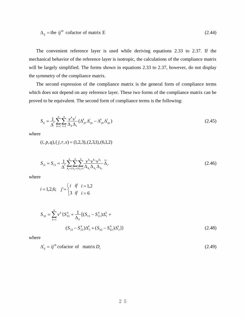
The second expression of the compliance matrix is the general form of compliance terms
which does not depend on any reference layer. These two forms of the compliance matrix can be
proved to be equivalent. The second form of compliance terms is the following:
∑∑= =
ΔΔ−ΔΔΔΔΔ
=n
k
n
l
lqs
kps
lqs
kpr
lk
lk
ijvvS
1 1* )(1 (2.45)
where
)2,1,6(),1,3,2(),3,2,1(),,(),,,( =srjqpi
∑∑∑= = =
ΔΔΔΔΔ
==n
k
n
k
n
ki
kkk
kkk
iivvvSS
1 1 1'*33
1 2 3 321
321 ~1 (2.46)
where
;6,2,1=i ⎩⎨⎧
=3
'i
j ifif
6
2,1==
ii
∑=
+Δ−Δ
+=n
k
kk
k
kk SSSvS1
113133333 )[(1{
]})()( 3636322323kkkk SSSS Δ−+Δ− (2.48)
where
=Δrij
thij cofactor of matrix rD (2.49)
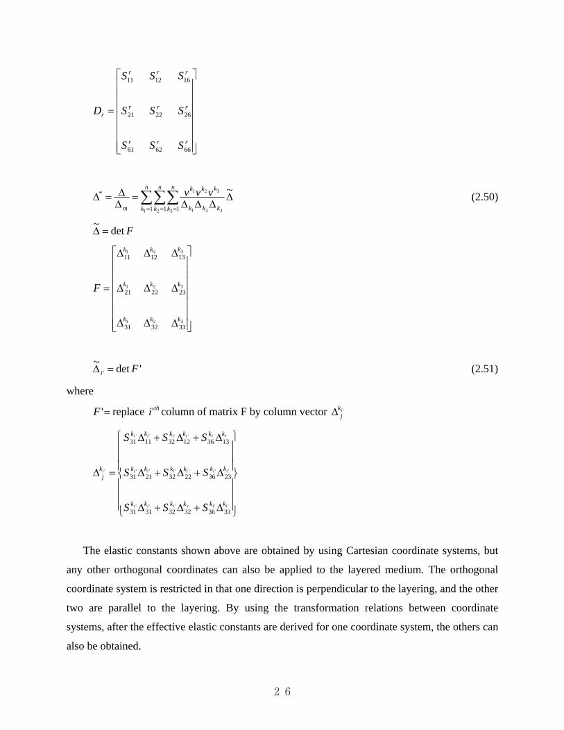
26
⎢⎢⎢⎢⎢⎢⎢
⎣
⎡
=
r
r
r
r
S
S
S
D
61
21
11
r
r
r
S
S
S
62
22
12
⎥⎥⎥⎥⎥⎥⎥
⎦
⎤
r
r
r
S
S
S
66
26
16
∑∑∑= = =
ΔΔΔΔ
=ΔΔ=Δ
n
k
n
k
n
k kkk
kkk
m
vvv1 1 1
*
1 2 3 321
321 ~ (2.50)
Fdet~ =Δ
⎢⎢⎢⎢⎢⎢⎢
⎣
⎡
Δ
Δ
Δ
=
1
1
1
31
21
11
k
k
k
F
2
2
2
32
22
12
k
k
k
Δ
Δ
Δ
⎥⎥⎥⎥⎥⎥⎥
⎦
⎤
Δ
Δ
Δ
3
3
3
33
23
13
k
k
k
'det~' Fi =Δ (2.51)
where
='F replace thi' column of matrix F by column vector 'ikjΔ
⎪⎪⎪
⎭
⎪⎪⎪
⎬
⎫
⎪⎪⎪
⎩
⎪⎪⎪
⎨
⎧
Δ+Δ+Δ
Δ+Δ+Δ
Δ+Δ+Δ
=Δ
''''''
''''''
''''''
'
333632323131
233622322131
133612321131
iiiiii
iiiiii
iiiiii
i
kkkkkk
kkkkkk
kkkkkk
kj
SSS
SSS
SSS
The elastic constants shown above are obtained by using Cartesian coordinate systems, but
any other orthogonal coordinates can also be applied to the layered medium. The orthogonal
coordinate system is restricted in that one direction is perpendicular to the layering, and the other
two are parallel to the layering. By using the transformation relations between coordinate
systems, after the effective elastic constants are derived for one coordinate system, the others can
also be obtained.

27
2.5 Verification Examples
The effective elastic moduli of laminated composites will be calculated in this section to
show the accuracy of the present approach. After obtaining the effective elastic compliance
matrix by the formulas in the previous section, the effective engineering moduli can be obtained
through the following relations:
11
1S
E x = 22
1S
E y = 33
1S
E z = (2.52)
22
23
SS
yz −=ν 11
31
SS
xz −=ν 11
21
SS
xy −=ν (2.53)
44
1S
G yz = 55
1S
G xz = 66
1S
G xy = (2.54)
where
[ ]
⎢⎢⎢⎢⎢⎢⎢⎢⎢
⎣
⎡
=
16
13
12
11
00
S
S
S
S
S
26
23
22
12
00
S
S
S
S
36
33
23
13
00
S
S
S
S
0
000
45
44
S
S
0
000
55
45
S
S
⎥⎥⎥⎥⎥⎥⎥⎥⎥
⎦
⎤
66
36
26
16
00
S
S
S
S
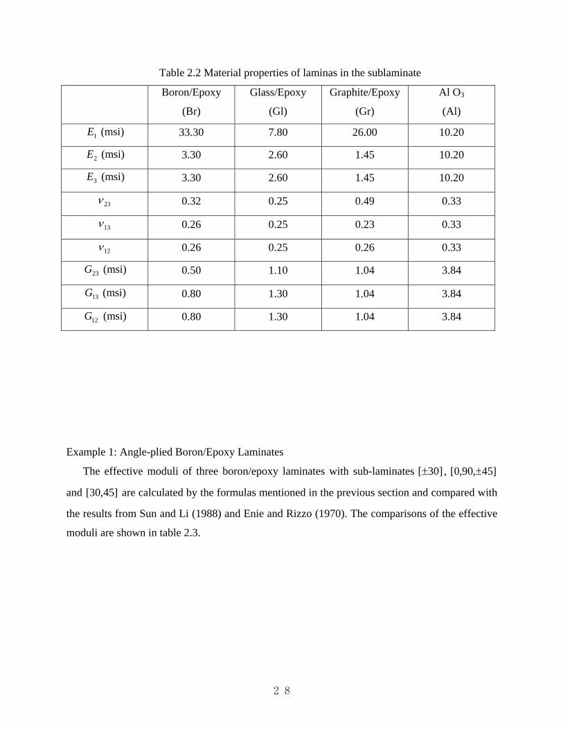
The material data used in the examples shown in this section are from Sun and Li (1988).
Table 2.2 shows the material properties used in the following examples.
28
Table 2.2 Material properties of laminas in the sublaminate
Boron/Epoxy
(Br)
Glass/Epoxy
(Gl)
Graphite/Epoxy
(Gr)
Al O3
(Al)
1E (msi) 33.30 7.80 26.00 10.20
2E (msi) 3.30 2.60 1.45 10.20
3E (msi) 3.30 2.60 1.45 10.20
23ν 0.32 0.25 0.49 0.33
13ν 0.26 0.25 0.23 0.33
12ν 0.26 0.25 0.26 0.33
23G (msi) 0.50 1.10 1.04 3.84
13G (msi) 0.80 1.30 1.04 3.84
12G (msi) 0.80 1.30 1.04 3.84
Example 1: Angle-plied Boron/Epoxy Laminates
The effective moduli of three boron/epoxy laminates with sub-laminates ]30[± , ]45,90,0[ ±
and ]45,30[ are calculated by the formulas mentioned in the previous section and compared with
the results from Sun and Li (1988) and Enie and Rizzo (1970). The comparisons of the effective
moduli are shown in table 2.3.

29
Table 2.3 Comparison of effective moduli for boron/epoxy angle-plied laminates
Effective Moduli ]30[± ]45,90,0[ ± ]45,30[
Chou et al. (1972) 10.4 12.8 4.48
Sun and Li (1988) 10.4 12.8 4.60 xE (msi)
Enie and Rizzo
(1970) 10.34 12.8 4.48
Chou et al. (1972) 2.54 12.8 3.39
Sun and Li (1988) 2.54 12.8 3.37 yE (msi)
Enie and Rizzo
(1970) 2.54 12.8 3.39
Chou et al. (1972) 3.42 3.57 3.30
Sun and Li (1988) 3.42 3.57 3.31 zE (msi)
Enie and Rizzo
(1970) 3.33 3.57 3.31
Chou et al. (1972) 0.216 0.224 0.215
Sun and Li (1988) 0.216 0.224 0.215 yzν
Enie and Rizzo
(1970) 0.183 0.212 0.159
Chou et al. (1972) -0.125 0.224 0.179
Sun and Li (1988) -0.125 0.224 0.175 xzν
Enie and Rizzo
(1970) 0.112 0.212 0.123

30
Table 2.3 Comparison of effective moduli for boron/epoxy angle-plied laminates (Continued)
Effective Moduli ]30[± ]45,90,0[ ± ]45,30[
Chou et al.
(1972) 1.40 0.336 0.459
Sun and Li
(1988) 1.40 0.336 0.472 xyν
Enie and Rizzo
(1970) 1.39 0.336 0.255
Chou et al.
(1972) 0.552 0.615 0.582
Sun and Li
(1988) 0.552 0.615 0.582 yzG (msi)
Enie and Rizzo
(1970) 0.555 0.615 0.582
Chou et al.
(1972) 0.696 0.615 0.653
Sun and Li
(1988) 0.696 0.615 0.653 xzG (msi)
Enie and Rizzo
(1970) 0.695 0.615 0.653
Chou et al.
(1972) 6.78 4.79 2.55
Sun and Li
(1988) 6.79 4.79 2.62 xyG (msi)
Enie and Rizzo
(1970) 6.72 4.79 2.55
31
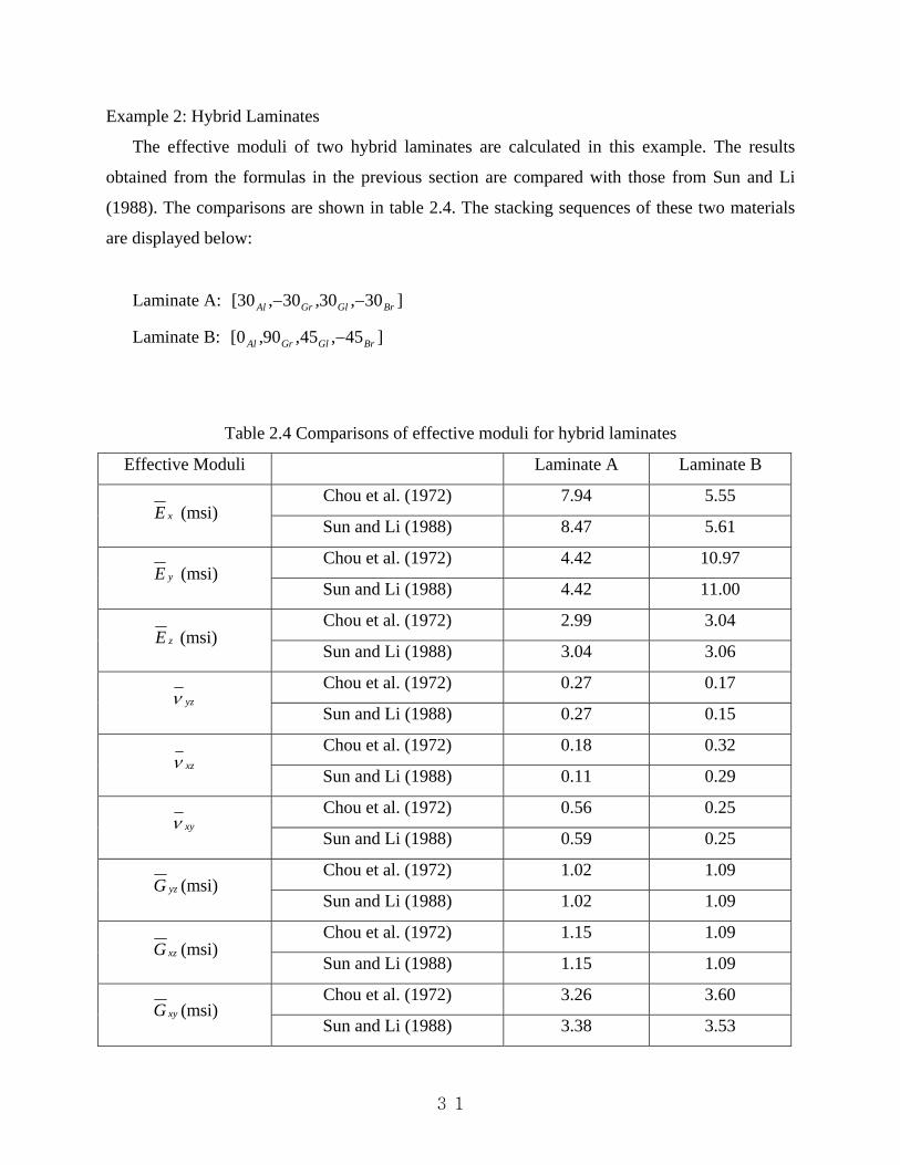
Example 2: Hybrid Laminates
The effective moduli of two hybrid laminates are calculated in this example. The results
obtained from the formulas in the previous section are compared with those from Sun and Li
(1988). The comparisons are shown in table 2.4. The stacking sequences of these two materials
are displayed below:
Laminate A: ]30,30,30,30[ BrGlGrAl −−
Laminate B: ]45,45,90,0[ BrGlGrAl −
Table 2.4 Comparisons of effective moduli for hybrid laminates
Effective Moduli Laminate A Laminate B
Chou et al. (1972) 7.94 5.55 xE (msi)
Sun and Li (1988) 8.47 5.61
Chou et al. (1972) 4.42 10.97 yE (msi)
Sun and Li (1988) 4.42 11.00
Chou et al. (1972) 2.99 3.04 zE (msi)
Sun and Li (1988) 3.04 3.06
Chou et al. (1972) 0.27 0.17 yzν
Sun and Li (1988) 0.27 0.15
Chou et al. (1972) 0.18 0.32 xzν
Sun and Li (1988) 0.11 0.29
Chou et al. (1972) 0.56 0.25 xyν
Sun and Li (1988) 0.59 0.25
Chou et al. (1972) 1.02 1.09 yzG (msi)
Sun and Li (1988) 1.02 1.09
Chou et al. (1972) 1.15 1.09 xzG (msi)
Sun and Li (1988) 1.15 1.09
Chou et al. (1972) 3.26 3.60 xyG (msi)
Sun and Li (1988) 3.38 3.53

32
Chapter 3 Torsional Response of Laminated Composite Beam
3.1 Introduction
The elastic response of inhomogeneous beams is often of interest in many engineering
fields (Savoia and Tullini, 1993). In this chapter, the elastic response of an arbitrarily shaped
composite beam will be analyzed. By employing Prandtl’s stress function, the expressions for
shear stress distribution, cross-sectional warping, and torsional rigidity can be determined. The
warping behavior is the beginning of the analyses of composite beams under a variety of loading
and boundary conditions. This chapter also presents the theoretical solution of the response of a
multilayered orthotropic beam under uniform torsion loading. The solution is in the form of a
series, which is a similar form with the classical elasticity solution of an orthotropic rectangular
beam. Previous works about torsional response of composite beams include a two-layer bonded
isotropic beam (Muskhelishvili, 1963), isotropic symmetric sandwich beam (Cheng et al., 1989),
homogeneous anisotropic beam (Lekhnitskii, 1963) and orthotropic laminated beams (Tsai et al.,
1990). The last paper mentioned above proposes a Reissner-Mindlin theory approach to predict
the torsional behavior of orthotropic laminates. The result was compared with the exact solutions,
and it shows that the Reissner-Mindlin approach doesn’t approximate the torsional behavior well.
The shortcoming of this approach is that it underestimates the torsional stiffness of thick
laminates with a small number of plies and very distinct elastic properties.
Because of the high stiffness and strength to weight ratio, fiber composite materials have
become more and more important for industrial applications. For classical elasticity and
mechanics of materials problems of orthotropic laminated composites, the solutions are readily
available. The bending and axial loading behavior can be easily determined (Hyer, 1998). The
solution of torsional response of a rectangular isotropic homogeneous beam can be found in a
classical elasticity book (Timoshenko and Goodier, 1970). The solution of a rectangular
homogeneous orthotropic beam can also be determined (Lekhnitskii, 1981). The derivation of the
isotropic solution is based on the membrane analogy. This approach can be applied to the
solution of open cross sections, such as U shape, I shape, and T shape. A similar approach can be
employed in the orthotropic laminated composite beams.
33
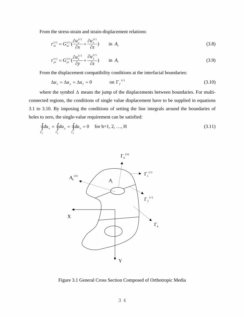
3.2 General Formulation
A general cross section of a prismatic bar composed of orthotropic material is considered
(Figure 3.1). The right hand orthogonal coordinate system (X, Y, Z) is used to analyze the beam.
The X-Y plane lies in the plane of Z=0, and the Z axis is along the centroidal axis. The cross
section is composed of many regions and holes, the area of the region is denoted as rA , and the
corresponding external boundary and interface boundary as )(rsΓ and )(r
fΓ respectively. The
orthotropic axis of each region is assumed to coincide with the reference axis. The area and
boundary of the n-th hole are denoted as )(nhA and )(n
hΓ respectively. Two assumptions have to
made, that the boundary )(rΓ of r-th region is a piecewise curve, and that the same interface is
not shared by more than two regions. The St. Venant torsion problem is considered here. The
problem states that the resultants of two ends of the prismatic bar are produced by the tangential
shear stress distributions, and can be considered as the problem under a twisting torque T. By the
following elasticity conditions, the governing differential equations can be derived.
From the equilibrium equation:
0)()(
=∂∂
+∂∂
yx
ryz
rxz ττ
in rA (3.1)
From the traction-free equations for the lateral boundaries:
0)()( =+ yr
yzxr
xz nn ττ on )(rsΓ (3.2)
From the traction-free equations for the boundaries of holes:
0)()( =+ yr
yzxr
xz nn ττ on )(rsΓ (3.3)
From the stress continuity condition at the layer interfaces:
0)( )()( =+Δ yr
zyxr
zx nn ττ (3.4)
where Δ stands for the jump of the values between layer interfaces.
From stress balance at the ends of the beam:
∫∫ =A
xz dA 0τ (3.5)
∫∫ =A
yz dA 0τ (3.6)
TdAyxA
xzyz =−∫∫ )( ττ (3.7)
34
From the stress-strain and strain-displacement relations:
)()()(
)()(
zu
xu
Gr
xr
zrxz
rxz ∂
∂+
∂∂
=τ in rA (3.8)
)()()(
)()(
zu
yuG
ry
rzr
yzr
yz ∂∂
+∂∂
=τ in rA (3.9)
From the displacement compatibility conditions at the interfacial boundaries:
0=Δ=Δ=Δ zyx uuu on )(rfΓ (3.10)
where the symbol Δ means the jump of the displacements between boundaries. For multi-
connected regions, the conditions of single value displacement have to be supplied in equations
3.1 to 3.10. By imposing the conditions of setting the line integrals around the boundaries of
holes to zero, the single-value requirement can be satisfied:
∫ ∫ ∫Γ Γ Γ
===h h h
zyx dududu 0 for h=1, 2, …, H (3.11)
Figure 3.1 General Cross Section Composed of Orthotropic Media
Y
X
rA
)(rfΓ
)(rsΓ
)(nhΓ
)(nhA
hΓ
35
3.3 Formulation for Orthotropic Composite Beams
The problem of equations 3.1 to 3.10 can be solved by either use of the warping function or
in terms of the Prandtl’s stress function. Two assumptions have to be made: the first one is that
the plane of the cross section remains plane, and the second one is that the plane has warping
deformation which is assumed to be a constant value along the axial direction of beam. From the
above assumptions, the displacements can be expressed as
θyzux −=
θxzu y = (3.12)
θ),()( yxwu rr
z =
where θ is the angle of twist per unit beam length and rw is the warping function of the r-th
layer. Introducing equation 3.11 in equations 3.7 and 3.8, the stress components can be shown in
the form
)()()( yx
wG rr
zxr
zx −∂∂
= θτ (3.13)
)()()( xy
wG rrzy
rzy +
∂∂
= θτ (3.14)
Substituting equations 3.12 and 3.13 into equation 3.1, the generalized Laplace equation for
the r-th region can be determined:
02
2)(
2
2)( =
∂∂
+∂∂
ywG
xwG rr
zyrr
zx in rA (3.15)
Equation 3.14 can be reduced to a harmonic function if the material property is transversely
isotropic, where zyzx GG = . Substituting equations 3.12 to 3.14 into equations 3.2, 3.3, 3.4, 3.10,
3.11, the traction-free equations for the lateral and the hole boundary conditions become
yr
zyxr
zxyrr
zyxrr
zx xnGynGny
wGnx
wG )()()()( −=∂∂
+∂∂ on )(r
sΓ (3.16)
yr
zyxr
zxyrr
zyxrr
zx xnGynGny
wGnx
wG )()()()( −=∂∂
+∂∂ on )(n
hΓ (3.17)
The stress continuity condition at the interfaces of layers becomes
][][ )()()()(y
rzyx
rzxy
rrzyx
rrzx xnGynGn
ywGn
xwG −Δ=
∂∂
+∂∂
Δ on )(rfΓ (3.18)
36
The condition of displacement compatibility at the interfaces becomes
0=Δ rw on )(rfΓ (3.19)
The condition of vanishing of the line integral along the closed loop hΓ surrounding a hole
of the cross section becomes
∫ ∑ ∫Γ Γ
=∂∂
+∂∂
=h
rh
s
rr dyy
wdxx
wdw)(
0][ for h=1,…,H (3.20)
The uniform torsion problem can also be formulated by the Prandtl’s stress function.
Assume rφ is the Prandtl stress function of the r-th layer. In order to satisfy the equilibrium
equation, the relations between shear stress and the Prandtl’s stress function for r-th layer can be
defined as
yrr
zx ∂∂
=φ
θτ )( (3.21)
xrr
zy ∂∂
−=φ
θτ )( (3.22)
By equating equations 3.21 and 3.22 with equations 3.13 and 3.14, the relation between the
warping function and Prandtl stress function for layer r can be obtained:
yyGx
w rr
zx
r +∂∂
=∂∂ φ
)(1 (3.23)
xxGy
w rr
zy
r −∂∂
−=∂∂ φ
)(1 (3.24)
By employing the following equality, the governing equations for the r-th layer can be
writtern in terms of the Prandtl’s stress function:
xyw
yxw rr
∂∂∂
=∂∂
∂ 22
(3.25)
2112
2
)(2
2
)( −=∂∂
+∂∂
yGxGr
rzx
rr
zy
φφ in rA (3.26)

37
3.4 Analytical Model for Rectangular Laminated Composites
Figure 3.1 shows the cross-section of a rectangular laminated composite beam with
dimensions 2b and 2h in the x and y directions respectively (Swanson, 1998). The layering is
parallel to the x axis, and the x-axis is also the symmetric axis of the composite. The material
characteristic of each layer is considered as orthotropic material behavior and is dominated by
two shear moduli, in the in-plane ( xzpG ) and through-thickness ( yxpG ) directions. The subscript p
is the p-th layer and the total number of layers is n. The classical lamination theory will be used
to obtain the shear moduli for both in-plane and through-thickness properties.
While obtaining the in-plane shear modulus xzpG , only the x and z coordinates will be
considered. The stress-strain relations for plane stress can be defined as (Hyer, 1998)
{ } [ ]{ }εσ Q= (3.27)
or
⎪⎭
⎪⎬
⎫
⎪⎩
⎪⎨
⎧
12
2
1
τσσ
=⎢⎢⎢
⎣
⎡
012
11
022
12
⎥⎥⎥
⎦
⎤
66
00
Q
⎪⎭
⎪⎬
⎫
⎪⎩
⎪⎨
⎧
12
2
1
γεε
(3.28)
where
2112
1111 1 νν−=
EQ
2112
121
2112
21212 11 νν
ννν
ν−
=−
=EEQ
2112
222 1 νν−=
EQ
1266 GQ =
The transformation matrix for a fiber-oriented composite can be given as
[ ] [ ][ ][ ][ ][ ]11 −−= RTRQTQ (3.29)
where
[ ]R =⎢⎢⎢
⎣
⎡
001
010
200
⎥⎥⎥
⎦
⎤ (3.30)
38
⎢⎢⎢
⎣
⎡=][T
mnnm
−
2
2
mnmn
2
2
22
22
nmmn
mn
−
− ⎥⎥⎥
⎦
⎤ (3.31)
θcos=m
θsin=n
Matrix R is used for transforming tensor shear strain to engineering shear strain. The in-
plane shear modulus xzpG can be obtained by transformation matrix Q.
Through-thickness shear moduli 13G and 23G can also be employed to obtain the through-
thickness shear properties of laminated composites. Again, the classical lamination theory will be
used. The shear stress-strain relation can be defined as
⎩⎨⎧
13
23
ττ
⎭⎬⎫
= ⎢⎣
⎡
023G
13
0G ⎥
⎦
⎤ ⎩⎨⎧
13
23
γγ
⎭⎬⎫
(3.32)
The through-thickness shear modulus yzG can then be obtained by
θθ 223
213 sincos GGGyz += (3.33)
The material property of each layer of the laminated composite beam is considered as
orthotropic. In order to maintain this material behavior, each layer has consisted of well
dispersed θ± angle fibers.

39
Figure 3.2 Cross-section of laminated composites
The displacements of each layer are assumed to be the same and can be expressed as
θyzux −=
θxzuy = (3.34)
θψ ),( yxu pz −=
where xu , yu , and zu are the displacements in x, y, and z directions, respectively, θ is the
angle of twist per unit length, and ),( yxpψ is the warping function of layer p. Substituting
equation 3.34 into the strain-displacement relations, the strain of layer p can be shown to be
h
h
X
Y
b b
p=1
p=n
nb

40
)( yxp
xz −∂∂
=ψ
θγ (3.35)
)( xyp
yz +∂∂
=ψ
θγ (3.36)
Substituting equation 3.35 and equation 3.36 into the stress-strain relations, the stress of
layer p can be obtained:
)( yxG pxzpxz −
∂∂
=ψ
θτ (3.37)
)( xyG pyzpyz +
∂∂
=ψ
θτ (3.38)
The relation between the stress and the Prandtl’s stress function for layer p can be defined
as
yp
xz ∂∂
=φ
τ (3.39)
xp
yz ∂∂
−=φ
τ (3.40)
Substituting equation 3.39 and equation 3.40 into equation 3.37 and equation 3.38,
respectively, the governing equation for layer p can be found:
θφφ
2112
2
2
2
−=∂
∂+
∂
∂
xGyGp
yzp
p
xzp (3.41)
In order to solve the governing equation, the continuity condition between each layer has to
be employed. The first condition is that the displacement zu must be continuous at the interfaces
of each layer. Hence, the warping function and the warping function derivative with respect to x
are also continuous at the boundary between each layer. By substituting equation 3.39 into
equation 3.37, the first continuity condition can be obtained:
11
1
1
11
−− =
−
−=∂
∂=
∂∂
pp by
p
xzpby
p
xzp yGyGφφ
(3.42)
The second continuity condition is that the shear stress yzτ has to be continuous at the
interface of each layer. From equation 3.40, the second continuity condition can be obtained:

41
11
1
−− =
−
=∂
∂=
∂∂
pp by
p
by
p
xxφφ
(3.43)
Since the stress function derivative with respect to x has to be continuous at the interface of
each layer, the stress function must also be continuous between the boundaries of each layer.
This condition leads us to the following equation:
111
−− =−==
pp bypbyp φφ (3.44)
The stress boundary condition has to be employed also, i.e., the stress at the outside of the
boundary will vanish. Hence, the shear stress xzτ must equal zero at the boundaries bx ±= , and
the shear stress yzτ must vanish at the edges hy ±= . From equations 3.39 and 3.40, the stress
function for each layer has a constant value at the edges of bx ±= , and the stress function for the
first and last layer must be constant at the boundaries hy ±= .
In order to solve the governing equation with the associated boundary conditions, a similar
solving procedure to that in Lekhnitskii (1981) can be used. The assumed solution is taken as a
series form
)2cos(∑=n
pnp xbnF πφ (3.45)
The constant term in the governing equation can also be expanded into a series form:
∑−=−n
n xbnS )2cos(2 πθθ (3.46)
Substituting equations 3.45 and 3.46 into the governing equation, the solution can be
obtained:
πnSn
n8)1( 2
1−−= , n=1, 3, 5, … (3.47)
θπ
αα yzp
n
pnpnpnpnpn Gn
byDyDyF 33
22
1
2132)1(sinhcosh)(
−
−++= (3.48)
where
bn
GG
yzp
xzppn 2
πα = (3.49)
The total solution can be obtained by introducing equation 3.48 into equation 3.45:
42
∑∞
=
−
−−−=,...5,3,1
32
1
3
2)2cos()sinhcosh1(1)1(32
npnpnpnpn
n
yzpp xbnyByA
nGb παα
πθφ (3.50)
The resultant torque acting on the end of the beam due to the shear stress distribution has to
be identical with the applied torsional moment. This leads us to the following equation:
xdxdyydxdydT yzxz ττ +−= (3.51)
Substituting the relations between shear stresses and stress function into equation 3.51, and
integrating over the whole cross-section of the beam, the total torque can be obtained:
dydxxx
yy
T ppb
b
h
h⎟⎟⎠
⎞⎜⎜⎝
⎛∂∂
+∂∂
−= ∫∫−−
φφ (3.52)
The equation mentioned above is satisfied within each individual layer. Integration in
equation 3.52 can be set equal to integration over each layer and summed up. By using the
technique of integration by parts,
∫ ∫∑− ⎥
⎥⎦
⎤
⎢⎢⎣
⎡−−=
−−
b
b
b
bp
b
bpp
dxdyyTp
p
p
p1
1)( φφ dydxx
b
bp
b
bp
b
bp
p
p
⎥⎦
⎤⎢⎣
⎡−− ∫∫∑
−−
−
φφ )(1
(3.53)
where pb and 1−pb are the locations of layers as shown in figure 3.1. The first b value is
equal to –b. From the boundary conditions, the stress function at the exterior boundary must be
constant value. In the laminated composite case, we assume it is equal to zero as employed in the
classical elasticity textbooks. Using the continuity condition that the stress function is continuous
at the interface in equation 3.53, the resulting equation is obtained as
∫∑∫∫∫−−−−
==p
p
b
bp
p
b
b
b
b
h
h
dxdydydxT1
22 φφ (3.54)
Applying equation 3.50 and condition 0=φ at the exterior boundary in equations 3.42 and
3.44, two equations can be obtained:
)coshsinh( 11 −− − ppnpnppnpnpnxzp
yzp bBbAGG
ααα
)coshsinh( 1,1,11,1,1,11
1−−−−−−−
−
− −= pnpnppnpnpnpxzp
yzp bBbAGG
ααα (3.55)
)sinhcosh1( 11 −− −− ppnpnppnpnyzp bBbAG αα
)sinhcosh1( 1,1,11,1,11 −−−−−−− −−= pnpnppnpnpyzp bBbAG αα (3.56)
43
If the layering of the laminated composite is symmetric with respect to the center line, the
constant pnB will vanish, and the simple form of the constants nA1 and pnA can be expressed as
hAn
n1
1 cosh1α
= (3.57)
⎥⎦
⎤⎢⎣
⎡−−= −−
−−
)cosh1(1cosh1
1,111
ppnnpyzp
yzp
ppnpn bAG
GbA α
α (3.58)
Substituting equations 3.57 and 3.58 into equation 3.50, the explicit solution for the stress
function can be obtained. Then performing the integration in equation 3.54, the total torque can
be determined:
∑ ∑∞
=
=p n
yzp nGahbT
,...5,3,144
31)()2(32
πθ
⎩⎨⎧
−−−
−− )sinh(sinh22 11
ppnppnpn
pnpp bbhA
hbb
ααα
⎭⎬⎫
−− − )cosh(cosh2 1ppnppnpn
pn bbhB
ααα
(3.59)
The effective torsional rigidity can be obtained as
∑ ∑∞
=
=p n
yzp nGahbGJ
,...5,3,144
31)()2(32
π
⎩⎨⎧
−−−
−− )sinh(sinh22 11
ppnppnpn
pnpp bbhA
hbb
ααα
⎭⎬⎫
−− − )cosh(cosh2 1ppnppnpn
pn bbhB
ααα
(3.60)
By introducing equation 3.50 in equation 3.39 and 3.40, and employing the relationGJT=θ ,
the shear stresses can be determined as
yzpxz TGGJbyx 2
16),(π
τ −=
[ ]∑∞
=
−
+−
,...5,3,12
21
2coscoshsinh)1(n
pnpnpnpn
n
xbnyByA
nπαα (3.61)
44
yzpyz TGGJbyx 2
16),(π
τ =
[ ] xbnyByA
nnpnpnpnpn
n
2sinsinhcosh1)1(,...5,3,1
2
21
παα∑∞
=
−
−−− (3.62)
Shear stresses at the mid-point of the boundary can also be obtained as
( )hBhAn
GGTGJbh pnpnpnpn
n
n
xzpyzpxz ααπ
τ coshsinh)1(16),0(,...5,3,1
2
21
2 +−
= ∑∞
=
−
(3.63)
⎟⎟⎠
⎞⎜⎜⎝
⎛−= ∑
∞
= ,...5,3,122
812)0,(n
pnyzpyz n
AG
GJbTb
πτ (3.64)

45
Chapter 4 Finite Element Analysis
4.1 Introduction
By employing the laws of physics, physical phenomena appearing in nature can be
formulated in mathematical forms which include algebraic equations, differential equations, and
integral equations (Reddy, 2006). The physical phenomena mentioned here may include the
range of biology, geology, and mechanics. Examples can be shown in the following real-world
problems. For example, the search of pollutants in the river, seawater, or the atmosphere, the
determination of stress distribution in a pressure vessel that is subjected to thermal, mechanical,
and aerodynamic loading, the formulation of tornados and thunderstorms. Two major stages are
involved in the study of physical phenomena: the first one is the mathematical formulation, and
the second is analyzing the mathematical model gained from the first step by employing
numerical methods.
Mathematical methods and laws of physics are required to formulate a physical problem
into a mathematical form. The resulting mathematical forms usually appear as differential
equations. These kinds of equations often contain physical quantities which researchers are
interested in to solve the physical problem or apply into design work. Certain assumptions have
to be made in order to simplify the complex physical phenomena and develop suitable
mathematical models. By employing numerical methods and computers, researchers can simulate
the mathematical models and understand the characteristics of the physical process.
The derived governing differential equations are often unable to be solved by traditional
analytical methods. When encountering these situations, approximate or numerical methods
become the only route to solve the governing equations. Two methods are usually considered as
effective methods. These are the finite difference method and variational methods such as the
Galerkin method and the method of Rayleigh-Ritz. The finite difference formulations of the
differential equations are developed by replacing the differential equations with the finite
difference quotients which contain the function values at each mesh point of the domain. The
function values at each mesh point of the domain can be determined by solving the algebraic
equations with associated boundary conditions. By employing the variational method in the
governing differential equations, the equations are in terms of equivalent weighted-integral forms
and the approximate solutions of the governing equations are assumed to a be linear combination

46
of approximation functions, with unknown coefficients. These unknown coefficients are
determined so that the integral form is equivalent with the governing differential equation.
Depending on different choices of integral form and approximation functions, the variational
method can be divided into many sub-division methods which include Rayleigh-Ritz method,
Galerkin method, and least squares method. These traditional variational methods will become
ineffective for the problems involving an arbitrary domain. The shortcoming is that the
approximation functions will be difficult to formulate in these types of problems.
The advantage of the finite element method over the traditional variational methods is that
it overcomes the disadvantage of constructing the approximation functions over the complex
domain. A systematic procedure of formulating the weighting function or approximation
function in the sub-domain, which is usually a simple domain, is employed in the finite element
analysis. There are three main reasons that make the finite element method more suitable for
complex problem than other traditional numerical methods. First, instead of formulating the
whole complex domain at once, the complex domain is formulated with an assembly of simple
geometrical sub-domains, called finite elements. Second, the approximating functions are
derived by employing functions that can be represented as a combination of algebraic
polynomials. Third, for each element, the unknown coefficients can be determined by equating
the algebraic relations with the governing equations which are in the weighted-integral form.
From the perspective mentioned above, the finite element method can also be considered as an
application of element combinations of the Rayleigh-Ritz method or weighted-residual method.
The approximating functions are usually in the form of polynomials, and the unknown
coefficients are the values at nodal points. The nodal points exist in the interior and boundary of
the elements. The approximating functions are sometimes called interpolation functions because
the derivation of the approximation functions uses the theory of interpolation. The choices of the
number of nodes and the orders of the differential equations will influence the degree of
interpolation functions.
Although the term finite element method is used in the present, the idea behind it is not
new. The ancient mathematicians used a similar concept to approximate the value of π by
inscribing a polygon in a circle. By increasing the number of the sides of the polygon inscribed
in a circle, the value of π can be approximated to the very high degree of accuracy. In the present
ages, the first application of the finite element method was found in the analysis of aircraft
47
structures. The analysis of wings of fuselages can be in terms of the analysis of combinations of
stringers, skins, and shear panels. A similar method, the framework method, was proposed by
Hrenikoff in 1941. In this paper, a plastic plane is treated as a combination of beams and bars.
Courant (1943) proposed to approximate an unknown function as an assembly of piecewise
continuous functions over simpler sub-domains. The St. Venant torsion problem is solved by
employing the minimum total potential energy principle and representing the whole domain by a
collection of triangular elements. Although similar concepts were proposed by the two authors
mentioned above, the formal literature contributed to Argyris and Kelsey (1960) and Turner et al.
(1956). The term finite element method was first used in the paper of Clough (1960). Since then,
the development, research, and applications of the finite element method have progressed very
fast. The historical review of the advancement of the finite element method can be found in
numerous books and journal papers. The application of the finite element method has expanded
to almost every science field.
The finite element method is a method that divides the whole complex domain into many
simple sub-domains, which are called finite elements, and constructs the approximating
functions over each element. There are two advantages of dividing the domain into piece-wise
connected domains. First, the complex domain can be accurately represented and the problem
involving dissimilar materials in the whole domain can be solved. Second, the solution over each
element can be accurately represented and problems involving local effects can be studied. Three
major finite element procedures can be stated. First, in order to represent the geometry and the
solution of the problem, the whole domain is divided into piece-wise connected simple domains.
Second, the approximated solution over each element is assumed to be a linear combination of
approximating functions and solution values at nodes. Third, through the algebraic relations, the
nodal solutions are determined, and then the solution over the whole domain can be obtained by
assembling the elements.
Despite the three major procedures, there are some detail features of the finite element
method. First, more than one type of element can be used when the dividing work is needed. For
example, a complex domain can be divided into a combination of triangular and rectangular
elements. Second, if more than one type of element is employed over the whole domain, the
development of approximating functions for each type of element should be executed separately.
Third, the governing equations are usually in the form of complex differential equations. The

48
equations may not be able to be solved for the following reasons. The exact solution cannot be
found; hence the traditional variational method should be used. The algebraic equations obtained
by a variational method cannot be solved without utilizing the appropriate continuity, boundary,
and initial conditions. Fourth, two major differences of the form of approximating functions can
be found between the use of the finite element method and traditional variational methods. For
example, the approximating function in variational methods is applied over the whole domain.
The first difference appears in the choice of unknown parameters in the linear combination of
approximating functions and undetermined coefficients. The traditional variational method uses
arbitrary parameters while the finite element method employs the solution value or the derivative
value at each nodal point. The second difference is that the approximating function in the finite
element method is often in the form of a polynomial that is derived from interpolation theory.
The approximate solution for the finite element method is usually in terms of a linear
combination of interpolation functions and nodal point values. The approximation function can
also be in terms of nodeless variables instead of nodal values.
The location and number of nodal points in one element depends on the following three
impact factors: first, the degree of the approximating polynomial; second, the form of the integral
in the governing equation; and third, the elemental geometry. The approximate solution can be
determined by representing the solution in terms of values at the nodal points. The idea of
assembling each element into the whole domain is used because the solution is assumed to be
continuous at the inter-element boundaries. Sometimes the condition of continuity of solution
uses solution derivatives instead. After assembling all finite elements, the boundary conditions
and initial conditions can then be applied to the problem. The equation for each finite element
can be solved by imposing the associated boundary conditions and initial conditions.
Errors in numerical methods are unavoidable. Knowing the source of errors makes it easier
to understand and decrease numerical errors. There are three major sources of numerical errors:
first, the error caused by approximating the domain; second, the error due to the approximation
of the problem solution; third, the error caused by numerical computation, including round-off
and numerical integration errors. The evaluation of error is not a easy task. For certain problems,
the error can be evaluated. Depending on the governing differential equations, the forms of
integrals, and the element employed, the accuracy and convergence of the solution in the finite
element method can be determined. The term accuracy means the difference between the

49
analytical solution and the solution obtained from the finite element method. The term
convergence means that increasing the number of elements will increase the accuracy of the
finite element solution and approach the exact solution.
Two major stages are involved when solving a time-dependent problem. In the first one,
the governing differential equation is approximated by the finite element method in order to gain
ordinary differential equations in time. In the second one, the obtained ordinary differential
equation is solved exactly by an analytical method or approximately by the finite difference
method or variational methods. The approximated equations are then in the form of algebraic
equations. The obtained algebraic equations can then be solved for the values at nodal points. A
similar numerical method is called the discrete element method, which uses contact conditions
instead of continuity conditions in the inter-element boundary. In this method, finite motions,
such as displacements and rotations, are permitted. The application of this method can be found
in rock mechanics, such as tunneling and mining engineering, and in ice mechanics.
Figure 4.1 2D rectangular beam cross section
Y
X
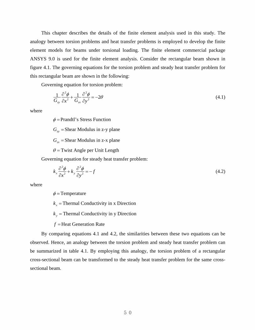
50
This chapter describes the details of the finite element analysis used in this study. The
analogy between torsion problems and heat transfer problems is employed to develop the finite
element models for beams under torsional loading. The finite element commercial package
ANSYS 9.0 is used for the finite element analysis. Consider the rectangular beam shown in
figure 4.1. The governing equations for the torsion problem and steady heat transfer problem for
this rectangular beam are shown in the following:
Governing equation for torsion problem:
θφφ 2112
2
2
2
−=∂∂+
∂∂
yGxG zxzy (4.1)
where
=φ Prandtl’s Stress Function
=zyG Shear Modulus in z-y plane
=zxG Shear Modulus in z-x plane
=θ Twist Angle per Unit Length
Governing equation for steady heat transfer problem:
fy
kx
k yx −=∂∂+
∂∂
2
2
2
2 φφ (4.2)
where
=φ Temperature
=xk Thermal Conductivity in x Direction
=yk Thermal Conductivity in y Direction
=f Heat Generation Rate
By comparing equations 4.1 and 4.2, the similarities between these two equations can be
observed. Hence, an analogy between the torsion problem and steady heat transfer problem can
be summarized in table 4.1. By employing this analogy, the torsion problem of a rectangular
cross-sectional beam can be transformed to the steady heat transfer problem for the same cross-
sectional beam.

51
Table 4.1 Analogy between Torsion Problem and Heat Transfer Problem
Torsion Problem Heat Transfer Problem
φ
(Stress Function)
φ
(Temperature)
zyG1
(The Reciprocal of Shear Modulus in z-y
Plane)
xk
(Thermal Conductivity in x Direction)
zxG1
(The Reciprocal of Shear Modulus in z-x
Plane)
yk
(Thermal Conductivity in y Direction)
θ2
(Twice the Angle of Twist Per Unit Length)
f
(Heat Generation)
yzτ−
(Minus the Shear Stress in y-z Plane) x∂
∂φ
(Temperature Gradient in x Direction)
xzτ
(Shear Stress in x-z Plane) y∂
∂φ
(Temperature Gradient in y Direction)

52
4.2 Finite Element Procedure
The ANSYS PLANE77 (2D 8-node Thermal Solid) element will be used in this study. This
element has one degree of freedom, temperature, at each node (ANSYS, 2004). Figure 4.2 shows
the geometry of the element PLANE77. This eight-node element not only can be used to model a
straight boundary but is suitable for modeling a curved boundary problem also. The steady-state
and transient thermal analyses are problems to which this 8-node thermal element can be applied.
Instead of using free meshing, a mapped meshing technique in ANSYS is used to mesh the plane
domain model into small elements. The advantage of mapped meshing is that it restricts the
element shape and the pattern of the meshing. Only rectangular or triangular elements can be
chosen since the mapped meshing technique is employed. In this study, the rectangular elements
will be used, since the analysis model is a rectangular shape domain and the selection of
rectangular elements usually results in better engineering results. The material property of the
analysis model can be specified by thermal conductivity in x and y directions for PLANE77
elements. The values of thermal conductivity in x and y direction are the reciprocal of shear
modulus in the z-y plane and z-x plane, respectively. The torsion problem states that along the
boundary of the beam, the stress function will be set to zero. By the analogy mentioned in table
4.1, the analysis model is set to be isolated. Hence, the temperature along the boundary of the
analysis model is set to be zero. The boundary conditions can be defined at the keypoints or
nodal points in ANSYS. In this study, since the model has been built and meshed, there is no
keypoint left in the modeling domain. The node points became the only choice and one can set
all the nodal points along the analysis model boundary to be zero. For the loading condition in
the heat transfer problem, the heat generation rate is specified to be twice the value of the angle
of twist per unit length. After solving the problem, the temperature at each nodal point can be
obtained. The torsional rigidity can be decided by summing the temperature values at each nodal
point.

53
Figure 4.2 PLANE77 Geometry
4.3 Verification Examples
Example 1: Torsional Parameters for Rectangular Cross Sections
The verification example shown in figure 4.3 is from a textbook (Boresi and Schmidt,
2003). The value of the torsional parameter from the textbook is compared with the value
obtained from the ANSYS finite element analysis. The analytical solution of this rectangular
cross section beam subjected to uniform torsional loading is shown below:
The torsional constant is expressed as
]2
tanh11921[3
)2()2(,...5,3,1
55
3
∑∞
=
−=n h
bnnb
hbhJ ππ
(4.3)
The other form of the torsional constant can be written as
13 )2()2( kbhJ = (4.4)
where
x x
x x
x
xx x K
N
J
L O
P
I
MX
Y

54
]2
tanh11921[31
,...5,3,1551 ∑
∞
=
−=n h
bnnb
hk ππ
(4.5)
1k = torsional parameter for rectangular cross section
Figure 4.3 Rectangular Cross Section
Table 4.2 Comparison of 1k value between analytical and ANSYS results
b/h 1.0 1.5 2.0 2.5 3.0 4.0 6.0 10
1k
(Boresi
and
Schmidt)
0.141 0.196 0.229 0.249 0.263 0.281 0.299 0.312
1k
(ANSYS) 0.1406 0.1957 0.2287 0.2493 0.2633 0.2808 0.2983 0.3123
hh
b
b
x
y

55
The expression of shear stress in two orthogonal directions can be shown as
∑∞
=
−−−=
,...5,3,1 2
2/)1(
2
2cosh
2sinh
2cos)1(
16n
n
zx
hbnn
yh
nxh
nhG
π
ππ
πθτ (4.6)
∑∞
=
−−−=
,...5,3,1 2
2/)1(
2
2cosh
2cosh
2sin)1(
162n
n
zy
hbnn
yh
nxh
nhGxG
π
ππ
πθθτ (4.7)
In order to determine the value of maximum shear stress in the torsional rectangular
member shown in figure 4.3, the case where b is greater than h is considered here. From the
membrane analogy, the maximum slope of the stress function occurs in the middle point of the
longer side. This means the maximum shear stress will appear at the same position. By
substituting the conditions hx = and 0=y into equations 4.6 and 4.7, the value of maximum
shear stress can be expressed as
0)0,( === yhxzxτ (4.8)
...]
23cosh9
1
2cos
1[162)0,( 2max ++−====
hb
hb
GhGhyhxzy πππθθττ (4.9)
In terms of the k value, the maximum shear stress can be expressed as
kGh ]2[max θτ = (4.10)
where
∑=
−=,...5,3,1 22
2cosh
181n
hbnn
kππ
The relation of applied torque and 1k value can be expressed as
)2()2( 31 bhGkT θ= (4.11)
By comparing equations 4.11 and 4.10, the relation of maximum shear stress and the
applied torque can be expressed with a new torsional parameter 2k :
)2()2( 22
max bhkT=τ (4.12)
where
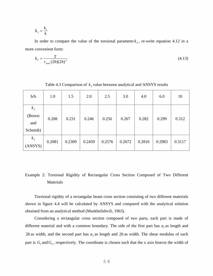
56
kk
k 12 =
In order to compare the value of the torsional parameter 2k , re-write equation 4.12 in a
more convenient form:
2max
2 )2)(2( hbTk
τ= (4.13)
Table 4.3 Comparison of 2k value between analytical and ANSYS results
b/h 1.0 1.5 2.0 2.5 3.0 4.0 6.0 10
2k
(Boresi
and
Schmidt)
0.208 0.231 0.246 0.256 0.267 0.282 0.299 0.312
2k
(ANSYS) 0.2081 0.2309 0.2459 0.2576 0.2672 0.2816 0.2983 0.3117
Example 2: Torsional Rigidity of Rectangular Cross Section Composed of Two Different
Materials
Torsional rigidity of a rectangular beam cross section consisting of two different materials
shown in figure 4.4 will be calculated by ANSYS and compared with the analytical solution
obtained from an analytical method (Muskhelishvili, 1963).
Considering a rectangular cross section composed of two parts, each part is made of
different material and with a common boundary. The side of the first part has 1a as length and
b2 as width, and the second part has 2a as length and b2 as width. The shear modulus of each
part is 1G and 2G , respectively. The coordinate is chosen such that the x axis bisects the width of

57
the rectangular cross section and the y axis is along the boundary interface between these two
different materials. Assuming the warping functions of each material are 1ϕ and 2ϕ , respectively,
the harmonic function for each part can be defined as
xy+= 11 ϕφ (4.14)
xy+= 22 ϕφ (4.15)
Figure 4.4 Rectangular Cross Section Composed of Two Different Materials
From the above definition of harmonic functions, the associated boundary conditions can
be found as follows:
yx
21 =∂∂φ
at 1ax −= and byb ≤≤− (4.16)
yx
22 =∂∂φ
at 2ax = and byb ≤≤− (4.17)
X
Y
b
b
1a 2a
1A 2A

58
)(2 212
21
1 GGyx
Gx
G −=∂∂
−∂∂ φφ
at 0=x and byb ≤≤− (4.18)
21 φφ = at 0=x and byb ≤≤− (4.19)
01 =∂∂
yφ at by ±= and 01 ≤≤− xa (4.20)
02 =∂∂
yφ at by ±= and 20 ax ≤≤ (4.21)
Satisfying all the boundary conditions mentioned above, the harmonic function of each part
can be determined as
myBA
nb
n
n
sin)12(
)1()2()2(1
1
03
321 ∑
∞
= +−
=π
φ (4.22)
myBA
nb
n
n
sin)12(
)1()2()2(2
2
03
322 ∑
∞
= +−
=π
φ (4.23)
where
)(cosh]cosh)([ 122121 axmmaGGGA +−+=
mxmaGmxmaG coshcoshsinhsinh 2122 −+
2121211 sinhcoshsinhcosh mamaGmamaGB +=
)(cosh]cosh)([ 212112 axmmaGGGA −−+−=
mxmaGmxmaG coshcoshsinhsinh 1211 ++
2121212 sinhcoshsinhcosh mamaGmamaGB +=
πb
nm2
12 +=
The warping functions of these two different parts can be determined from equations 4.14
and 4.15 as
xy−= 11 φϕ in 1A (4.24)
xy−= 22 φϕ in 2A (4.25)
Since the forms of both harmonic functions are known, the explicit forms of the warping
function for these two different parts can be shown as

59
xymyBA
nb
n
n
−+
−= ∑
∞
=
sin)12(
)1()2()2(1
1
03
321 π
ϕ (4.26)
xymyBA
nb
n
n
−+
−= ∑
∞
=
sin)12(
)1()2()2(2
2
03
322 π
ϕ (4.27)
The torsional rigidity of bars consisting of two different materials can be defined as
∫∫ ∂∂
−∂∂
++=1
)( 11221
A
dxdyx
yy
xyxGGJϕϕ
∫∫ ∂∂
−∂∂
+++2
)( 22222
A
dxdyx
yy
xyxG ϕϕ (4.28)
The explicit form of torsional rigidity of rectangular beam composed of two different
materials can then be determined:
∑ ∑∞
=
∞
=
−++=0 0 2
221
1
14532211 ][)4()(
38
n n DCGG
DCbbaGaGGJ
π (4.29)
where
212
22
112
222
11 coshcosh)(coshcosh mamaGGmaGmaGC +−+=
]sinhcoshsinhcosh[)12( 2121215
1 mamaGmamaGnD ++=
1)(coshcoshcosh 21212 −−−+= aammamaC
]sinhcoshsinhcosh[)12( 2121215
2 mamaGmamaGnD ++=

60
Case 1: Torsional rigidity with the change of the ratio of shear modulus 21 / GG
Parameters used in this case are as follows:
ma 41 = , ma 52 = , mb 5.1= , 22 /1 mNG =
The unit of torsional rigidity obtained here is 2mN −
Table 4.4 Comparison of torsional rigidity between analytical and ANSYS solutions
with the change of ratio of shear modulus 21 / GG
21 / GG 1.0 1.5 2.0 2.5
GJ
(Muskhelishvili) 63.9861 76.9984 88.9217 100.2226
GJ
(ANSYS) 63.9838 76.9955 88.9183 100.2186
Table 4.4 Comparison of torsional rigidity between analytical and ANSYS solutions
with the change of ratio of shear modulus 21 / GG (Continued)
21 / GG 3.0 3.5 4.0 4.5
GJ
(Muskhelishvili) 111.1345 121.7871 132.2581 142.5970
GJ
(ANSYS) 111.1300 121.7820 132.2525 142.5909

61
Case 2: Torsional rigidity with the change of the ratio of ba /1
Parameters used in this case are as follows:
ma 12 = , mb 1= , 21 /12 mNG = , 2
2 /24 mNG =
The unit of torsional rigidity obtained here is 2mN −
Table 4.5 Comparison of torsional rigidity between analytical and ANSYS solutions
with the change of ratio of ba /1
ba /1 1.0 1.5 2.0 2.5
GJ
(Muskhelishvili) 37.8176 54.0636 70.2765 86.3944
GJ
(ANSYS) 37.8112 54.0562 70.2681 86.3850
Table 4.5 Comparison of torsional rigidity between analytical and ANSYS solutions
with the change of ratio of ba /1 (Continued)
ba /1 3.0 3.5 4.0 4.5
GJ
(Muskhelishvili) 102.4525 118.4798 134.4925 150.4983
GJ
(ANSYS) 102.4421 118.4684 134.4801 150.4849

62
Case 3: Torsional rigidity with the change of the ratio of ba /2
Parameters used in this case are as follows:
ma 11 = , mb 1= , 21 /12 mNG = , 2
2 /24 mNG =
The unit of torsional rigidity obtained here is 2mN −
Table 4.6 Comparison of torsional rigidity between analytical and ANSYS solutions
with the change of ratio of ba /2
ba /2 1.0 1.5 2.0 2.5
GJ
(Muskhelishvili) 37.8176 62.5551 90.9069 121.1658
GJ
(ANSYS) 37.8112 62.5467 90.8965 121.153
Table 4.6 Comparison of torsional rigidity between analytical and ANSYS solutions
with the change of ratio of ba /2 (Continued)
ba /2 3.0 3.5 4.0 4.5
GJ
(Muskhelishvili) 152.3550 183.9818 215.8108 247.7327
GJ
(ANSYS) 152.3406 183.9654 215.7924 247.7123

63
Example 3: Torsional coefficients for orthogonal rectangular rod
Torsional coefficients of a rectangular beam cross section with two orthogonal shear
properties shown in figure 4.5 will be calculated by ANSYS and compared with the analytical
solution obtained from an analytical method (Lekhnitskii, 1963).
Consider a rectangular cross section beam with orthogonal material elasticity. One end of
the rectangular rod is fixed while the other end is subjected to a torsional moment T. The side of
the beam has lengths a and b, respectively. The solution of this problem can be solved by St.
Venant theory. The referring coordinates will change from the x-y system to the x’-y’ system.
From the theory, the shear stresses can be expressed as
yzx ′∂∂=′ ϕτ (4.30)
xzy ′∂∂−=′ ϕτ (4.31)
where
=ϕ Prandtl’s Stress Function
The governing equation for Prandtl’s stress function is
θϕϕ 2112
2
2
2
−=′∂
∂+′∂
∂yGxG zxzy
(4.32)

64
Figure 4.5 Cross Section of Orthogonal Beam
In order to satisfy the boundary conditions on two sides ( 0=′x and ax =′ ) of the
rectangular beam, the solution of the stress function is sought in the form
∑∞
=
′′=,...5,3,1
sin)(k
k xa
kyY πϕ (4.33)
Expanding the right hand side of equation 4.32 in a Fourier sine series in the interval between 0
and a, the governing equation can be rewritten as
∑∞
=
′−=′∂
∂+′∂
∂
,...5,3,12
2
2
2
sin1811kzxzy
xa
kkyGxG
πθπ
ϕϕ (4.34)
By substituting the expression for the stress function into equation 4.34, the function kY can then
be determined:
X
Y
a
b X ′
Y ′

65
kY
ak
GY
G kzy
kzx
18)(11 2 θπ
π −=−′′ (4.35)
The equation above is a second order ordinary differential equation in the function kY , hence the
function can be solved as
23)(
8coshsinh ak
ya
kBya
kAY kkk πθπμπμ +′+′= (4.36)
where
zy
zx
GG
=μ
The arbitrary constants kA and kB will be determined from the boundary conditions on the other
two sides ( 2/by =′ 2/by −=′ ) of the rectangular rod. The final expression for the stress
function can be shown as
xa
kBA
kaG
k
k
zyπ
πϕ cos)1()1(8
,...5,3,13
2/)1(2
3 −−
= ∑∞
=
−
(4.37)
where
ya
kA πμcosh=
abkB
2cosh πμ=
The torsional rigidity of the orthogonal rectangular rod can be obtained by the following
definition:
∫ ∫− −
=2/
2/
2/
2/
2a
a
b
b
GJ ϕ dxdy (4.38)
β3abGGJ zx= (4.39)
The applied torque can be shown as
θβzxGabT 3= (4.40)
where
∑∞
=
−=,...5,3,1
42
4 )2
tanh21(132k c
kckk
c πππ
β (4.41)

66
zx
zy
GG
bac = (4.42)
The shear stresses can be determined by employing the stress function in equations 4.30 and 4.31:
xa
kBA
kc
abT
k
k
zxπ
πτ cos)1(8
,...5,3,12
2/)1(
2 ∑∞
=
−−−= (4.43)
xa
kDC
kc
GG
abT
k
k
zx
zyzy
πβπ
τ sin)1()1(8,...5,3,1
2
2/)1(
22 −−
= ∑∞
=
−
(4.44)
where
ya
kA πμsinh=
abkB
2cosh πμ=
ya
kC πμcosh=
abkD
2cosh πμ=
Depending on the ratio of shear moduli and the ratio of the sides of the rectangular cross section
beam, the maximum shear stress may occur at the middle point of either side, i.e.
0=x and2by ±= , or
2ax ±= and 0=y . The maximum shear stress can be expressed as
32max kabT=τ at 0=x and
2by ±= (4.45)
or
42max kGG
abT
zx
zy=τ at 2ax ±= and 0=y (4.46)
where
∑∞
=
−
=,...5,3,1
2
2/)1(
23 2tanh)1(8
k
k
ck
kck π
βπ (4.47)
]
2cosh
181[,...5,3,1 224 ∑
∞
=
−=k
ckk
ckππβ
(4.48)

67
The analytical solution for torsional coefficients (β , 1k , 2k ) with the change of parameter c
obtained by equations 4.41, 4.47 and 4.48 will be compared with ANSYS results to show the
accuracy and effectiveness of the finite element method.
Table 4.7 Comparison of β value between analytical and ANSYS results
c 1 1.25 1.5 1.75 2 2.5
β
(Lekhnitskii) 0.141 0.172 0.196 0.214 0.229 0.249
β
(ANSYS) 0.1406 0.1717 0.1957 0.2142 0.2286 0.2493
Table 4.7 Comparison of β value between analytical and ANSYS results (continued)
c 3 4 5 10 20
β
(Lekhnitskii) 0.263 0.281 0.291 0.312 0.323
β
(ANSYS) 0.2633 0.2807 0.2912 0.3122 0.3226
Table 4.8 Comparison of 3k value between analytical and ANSYS results
c 1 1.25 1.5 1.75 2 2.5
3k
(Lekhnitskii) 4.804 4.521 4.330 4.186 4.068 3.882
3k
(ANSYS) 4.8044 4.5213 4.330 4.1861 4.0678 3.8829

68
Table 4.8 Comparison of 3k value between analytical and ANSYS results (continued)
c 3 4 5 10 20
3k
(Lekhnitskii) 3.742 3.550 3.430 3.202 3.098
3k
(ANSYS) 3.7423 3.5506 3.4301 3.2023 3.0982
Table 4.9 Comparison of 4k value between analytical and ANSYS results
c 1 1.25 1.5 1.75 2 2.5
4k
(Lekhnitskii) 4.804 4.141 3.767 3.434 3.234 2.975
4k
(ANSYS) 4.8044 4.1413 3.7671 3.4345 3.2342 2.9746
Table 4.9 Comparison of 4k value between analytical and ANSYS results (continued)
c 3 4 5 10 20
4k
(Lekhnitskii) 2.538 2.644 2.548 2.379 2.274
4k
(ANSYS) 2.5374 2.6437 2.5474 2.3784 2.2741

69
Chapter 5 Finite Difference Method
5.1 Introduction
The basic idea of the finite difference method is to represent the governing differential
equations and the associated boundary conditions with finite difference equations (Boresi et al.,
2003). The finite difference quotients are employed to approximate the derivatives in the
differential equations. Combinations of the values of unknown functions at the specified
locations of the independent variable form the finite difference quotients. The finite difference
equations with the specified values of the independent variables then lead to a system of
simultaneous algebraic equations that can be solved by computers.
To show how the difference quotients represent approximately the derivatives of the
differential equations, consider one simple case, one independent variable. Let y(x) be a function
of an independent variable x, where x is defined at ],[ 1 nbb . By dividing the domain into n-1 parts
(either equally or unequally), we get sub-dividing points nbbb ,...,, 21 called pivotal or nodal
points. By employing the interpolation polynomial theory, the n-th degree polynomial is assumed
to satisfy the conditions )()( iin bfbP = , i=1, 2, 3, …, n. The function y(x) can also be expressed
in terms of the sum of interpolation polynomial and remainder, )()()( xRxPxy nn += . Obviously
the derivative kn
kkn
kkk dxxRddxxPddxxyd /)(/)(/)( += , hence the derivative of the polynomial
is used to represent the derivative of the interpolation function y(x).
If the error in the derivative approximations can be observed, the accuracy of the
approximations is then easily found. By removing the error terms, the value of the derivative can
be expressed as kn
kkk dxxPddxxyd /)(/)( ≈ , where )(xPn is a linear combination of the
approximate values of )( iby , which can be denoted as )( ibY . Through the same procedure, all the
derivatives of the differential equations and boundary conditions can be replaced by the
corresponding finite difference equations. The formulation of the finite difference equations at
the specified nodal points will lead to a system of simultaneous algebraic equations in )( ibY . For
a linear boundary-value problem, the algebraic equations are a set of linear simultaneous
equations. For the nonlinear problem, a system of nonlinear equations will be obtained.

70
5.2 Finite Difference Equations
The basic expression of finite difference equation follows the rule of fundamental calculus
(Ugural and Fenster, 2003). The definition of the first derivative of function g(x) with respect to
the independent variable x can be expressed as (Figure 5.1)
xgg
xxgxxg
dxdg nn
x
nn
xn Δ−
=Δ
−Δ+= +
→Δ→Δ
1
00lim)()(lim)( (5.1)
where
n = any point on the curve
Instead of using infinitely small increments in the limit calculations, the finite difference
formulation assumes that the increment is a finite amount, denoted xhx =Δ . The expression of
equation 5.1 can then be expressed in an alternative form in the finite difference analysis:
x
n
x
nnn h
gh
ggdxdg Δ
=−
≈ +1)( (5.2)
By mathematical manipulations, the first forward difference at point nx can be defined as
nxnnn dxdghggg )(1 ≈−=Δ + (5.3)
Similarly, the first backward difference at point nx can be expressed as
nxnnn dxdghggg )(1 ≈−=∇ − (5.4)
The forward and backward difference analysis is usually employed for the nodal points on
the boundary when the central difference can not be used. The central difference method needs
three pivot points to formulate, which makes it more accurate than the forward and backward
difference formulations. By using pivot points forward and backward at the point nx , the first
derivative of function g(x) can be approximated by
)(21
2)()()( 11 −+ −=
−−+≈ nn
xx
xnxnn gghh
hxghxgdxdg (5.5)
By mathematical manipulations of equation 5.5, the first central difference can be
expressed as
nxnn dxdghggg )()(2
111 ≈−= −+δ (5.6)

71
Figure 5.1 Finite difference approximation of function g(x)
Similarly, by following the same procedure as the first difference formulation, the higher
order difference formulation can be derived. By employing equation 5.2 and equation 5.3, the
second-order derivative of function g(x) at pivot point nx can be expressed as
)(1)(1)()( 1222
2
nnx
nx
nn ggh
ghdx
dgdxd
dxgd −Δ=ΔΔ≈= + (5.7)
)(1)(1)(11212212 nn
xnn
xnn
x
ggh
ggh
ggh
−−−=Δ−Δ= ++++ (5.8)
)2(1122 nnn
x
gggh
+−= ++ (5.9)
By equating equation 5.7 and equation 5.9, the second forward difference at nodal point nx
can be derived as
nxnnnn dxgdhgggg )(2 2
22
122 ≈+−=Δ ++ (5.10)
1−nx
x
g(x)
xΔ xΔ
nx 1+nx
1−ng ng
1+ng

72
By employing equation 5.2 and equation 5.4, the second-order derivative of function g(x)
at the pivot point nx can be expressed as
)(1)(1)()( 1222
2
−−∇=∇∇≈= nnx
nx
nn ggh
ghdx
dgdxd
dxgd (5.11)
)(1)(1)(12121212 −−−− −−−=∇−∇= nn
xnn
xnn
x
ggh
ggh
ggh
(5.12)
)2(1212 −− +−= nnn
x
gggh
(5.13)
By equating equation 5.11 and equation 5.13, the second backward difference at nodal
point nx can be found as
nxnnnn dxgdhgggg )(2 2
22
212 ≈+−=∇ −− (5.14)
The coefficients of the nodal function values in the kth forward and backward differences
are the same as the coefficients of the binomial expansion kba )( − . Following the rules of
binomial expansion, the higher-order forward and backward differences can be easily obtained.
By employing the rule of equation 5.6, the second central difference at nodal point nx can
be obtained
)(21)(2
1)( 11112
−+−+ −=−== nnnnnn gggggg δδδδδδ
)](21)(2
1[21
22 −+ −−−= nnnn gggg
)2(41
22 −+ +−= nnn ggg (5.15)
The central difference value in equation 5.15 depends on the pivot function values at
second forward and backward nodal points. In order to improve the accuracy of the
approximations, the second central difference has to be evaluated by the first forward and
backward nodal point function values. By the following mathematical manipulations, the
transformation mentioned above can be done.
The following equality will be employed:
)(2nn gg ∇Δ=δ or )(2
nn gg Δ∇=δ (5.16)

73
The second central difference at pivot point nx can then be obtained by employing the
equality above.
112 )()( −− Δ−Δ=−Δ=∇Δ= nnnnnn ggggggδ
)()( 11 −+ −−−= nnnn gggg
11 2 −+ +−= nnn ggg
nx dxgdh )( 2
22≈ (5.17)
By following the same procedure, the third central difference can be displayed as
111123 2)2()( −+−+ +−=+−== nnnnnnnn gggggggg δδδδδδδ
)(21)()(
21
2112 −−++ −+−−−= nnnnnn gggggg
)22(21
2112 −−++ −+−= nnnn gggg
nx dxgdh )( 3
33≈ (5.18)
Similarly, the fourth central difference at the pivot point nx can be expressed as
122
12
112224 2)2()( −+−+ +−=+−== nnnnnnnn gggggggg δδδδδδδ
)2()2(2)2( 211112 −−−+++ +−++−−+−= nnnnnnnnn ggggggggg
2112 464 −−++ +−+−= nnnnn ggggg
nx dxgdh )( 4
44≈ (5.19)
It is easy to verify that the coefficients of the pivotal function values for even-order (kth-
order) central differences are exactly the same as the coefficients of the binomial
expansion kba )( − .
The extension of the finite difference method to two independent variables can be readily
derived. The partial differential equations are put in terms of finite difference equations by
employing the same technique used in the one independent variable case. In order to illustrate the
finite difference formulation for two independent variables, figure 5.2 will be used. By taking
xhx =Δ and yhy =Δ , a rectangular mesh is formed by the horizontal and vertical lines. The nodal
or pivotal points are the intersections of mesh lines.
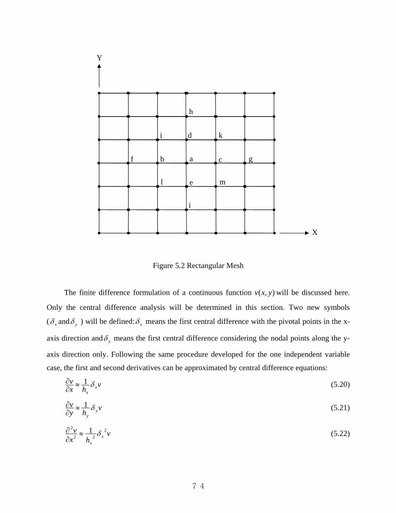
74
Figure 5.2 Rectangular Mesh
The finite difference formulation of a continuous function ),( yxv will be discussed here.
Only the central difference analysis will be determined in this section. Two new symbols
( xδ and yδ ) will be defined: xδ means the first central difference with the pivotal points in the x-
axis direction and yδ means the first central difference considering the nodal points along the y-
axis direction only. Following the same procedure developed for the one independent variable
case, the first and second derivatives can be approximated by central difference equations:
vhxv
xxδ1≈
∂∂ (5.20)
vhyv
yyδ1≈
∂∂ (5.21)
vhx
vx
x
222
2 1 δ≈∂∂ (5.22)
ab c
d
e
f g
h
i
j k
l m
X
Y

75
vhy
vy
y
222
2 1 δ≈∂∂ (5.23)
)(12
yv
hyxv
xx ∂
∂≈∂∂
∂ δ (5.24)
By associating with figure 5.2, equations 5.20 to 5.24 for the nodal point a can be re-
written as
)(21)],(),([2
1bc
xxx
xvvhyhxvyhxvhx
v −=−−+≈∂∂ (5.25)
)(21)],(),([2
1ed
yyy
yvvhhyxvhyxvhy
v −=−−+≈∂∂ (5.26)
)],(),(2),([122
2yhxvyxvyhxv
hxv
xxx
−+−+≈∂∂
)2(12 bac
x
vvvh
+−= (5.27)
)],(),(2),([122
2
yyy
hyxvyxvhyxvhy
v −+−+≈∂∂
)2(12 ead
y
vvvh
+−= (5.28)
)](21[12
edy
xx
vvhhyxv −≈∂∂
∂ δ
)(21
exdxyx
vvhh δδ −=
)](21)(2
1[21
lmjkyx
vvvvhh −−−=
)(41
lmfkyx
vvvvhh +−−= (5.29)
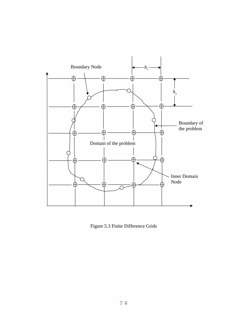
76
Figure 5.3 Finite Difference Grids
Domain of the problem
yh
xh
Boundary of the problem
Boundary Node
Inner Domain Node

77
5.3 Verification Examples
Three verification examples will be presented in this chapter. Instead of using the finite
element commercial package to produce the results, a numerical program employing the finite
difference method will be used. In order to provide the accuracy and efficiency of the finite
difference method, the results obtained from the numerical program will be compared with those
from the analytical method which is available from previous work.
Example 1: Torsional Parameters for Rectangular Cross Sections
Table 5.1 Comparison of 1k value between analytical and FDM results
b/h 1.0 1.5 2.0 2.5 3.0 4.0 6.0 10
1k
(Boresi
and
Schmidt)
0.141 0.196 0.229 0.249 0.263 0.281 0.299 0.312
1k
(FDM) 0.1404 0.1963 0.2289 0.2483 0.2627 0.2811 0.2983 0.3121
Table 5.2 Comparison of 2k value between analytical and FDM results
b/h 1.0 1.5 2.0 2.5 3.0 4.0 6.0 10
2k
(Boresi
and
Schmit)
0.208 0.231 0.246 0.256 0.267 0.282 0.299 0.312
2k
(FDM) 0.2076 0.2312 0.2464 0.2567 0.2667 0.2826 0.2993 0.3116

78
Example 2: Torsional rigidity of rectangular cross section composed of two different materials
Case 1: Torsional rigidity with the change of the ratio of shear modulus 21 / GG
Parameters used in this case are as follows:
ma 41 = , ma 52 = , mb 5.1= , 22 /1 mNG =
The unit of torsional rigidity obtained here is 2mN −
Table 5.3 Comparison of torsional rigidity between analytical and FDM solutions
with the change of ratio of shear modulus 21 / GG
21 / GG 1.0 1.5 2.0 2.5
GJ
(Muskhelishvili) 63.9861 76.9984 88.9217 100.2226
GJ
(FDM) 64.3677 75.8554 87.5213 101.5136
Table 5.3 Comparison of torsional rigidity between analytical and FDM solutions
with the change of ratio of shear modulus 21 / GG (Continued)
21 / GG 3.0 3.5 4.0 4.5
GJ
(Muskhelishvili) 111.1345 121.7871 132.2581 142.5970
GJ
(FDM) 112.3252 120.2129 134.2354 143.3424

79
Case 2: Torsional rigidity with the change of the ratio of ba /1
Parameters used in this case are as follows:
ma 12 = , mb 1= , 21 /12 mNG = , 2
2 /24 mNG =
The unit of torsional rigidity obtained here is 2mN −
Table 5.4 Comparison of torsional rigidity between analytical and FDM solutions
with the change of ratio of ba /1
ba /1 1.0 1.5 2.0 2.5
GJ
(Muskhelishvili) 37.8176 54.0636 70.2765 86.3944
GJ
(FDM) 37.1325 55.2135 70.5162 87.5621
Table 5.4 Comparison of torsional rigidity between analytical and FDM solutions
with the change of ratio of ba /1 (Continued)
ba /1 3.0 3.5 4.0 4.5
GJ
(Muskhelishvili) 102.4525 118.4798 134.4925 150.4983
GJ
(FDM) 103.1532 119.1526 135.5264 152.1151
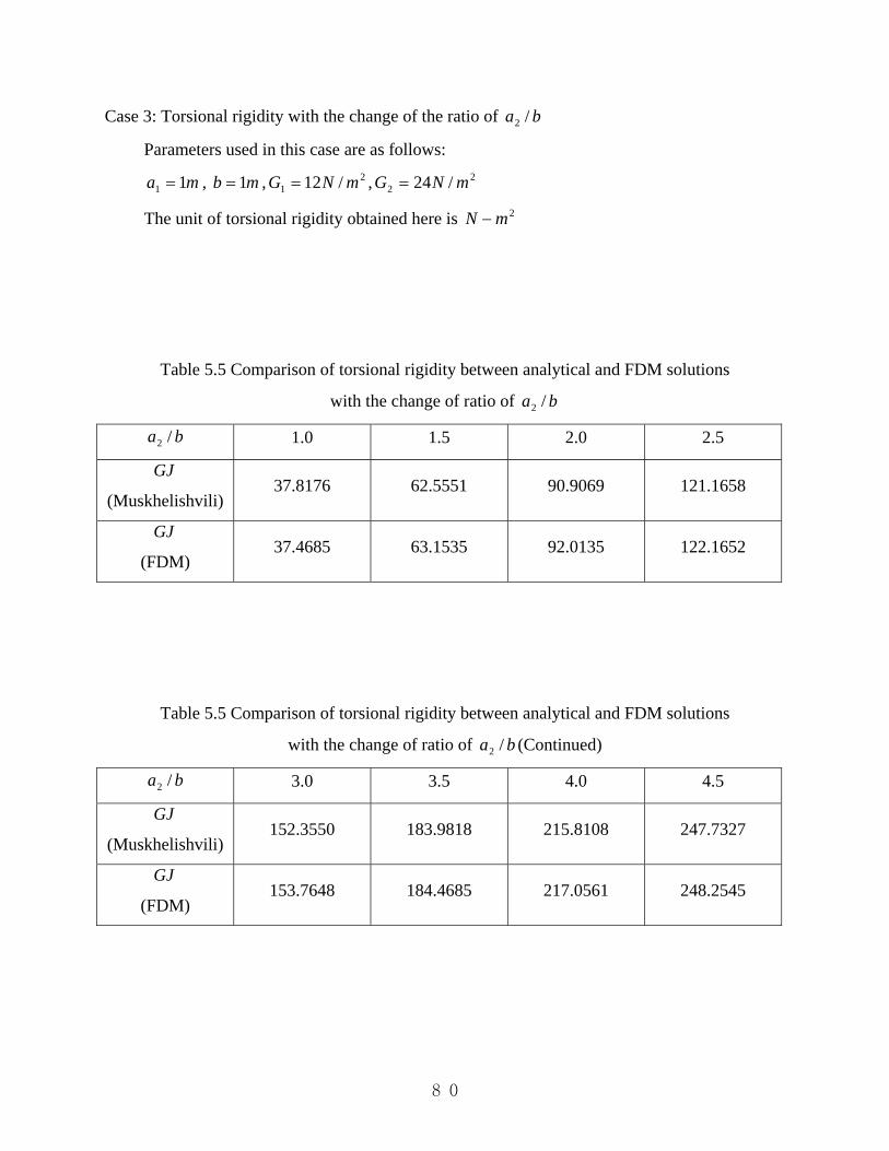
80
Case 3: Torsional rigidity with the change of the ratio of ba /2
Parameters used in this case are as follows:
ma 11 = , mb 1= , 21 /12 mNG = , 2
2 /24 mNG =
The unit of torsional rigidity obtained here is 2mN −
Table 5.5 Comparison of torsional rigidity between analytical and FDM solutions
with the change of ratio of ba /2
ba /2 1.0 1.5 2.0 2.5
GJ
(Muskhelishvili) 37.8176 62.5551 90.9069 121.1658
GJ
(FDM) 37.4685 63.1535 92.0135 122.1652
Table 5.5 Comparison of torsional rigidity between analytical and FDM solutions
with the change of ratio of ba /2 (Continued)
ba /2 3.0 3.5 4.0 4.5
GJ
(Muskhelishvili) 152.3550 183.9818 215.8108 247.7327
GJ
(FDM) 153.7648 184.4685 217.0561 248.2545

81
Example 3: Torsional coefficients for orthogonal rectangular rod
Table 5.6 Comparison of β value between analytical and FDM results
c 1 1.25 1.5 1.75 2 2.5
β
(Lekhnitskii) 0.141 0.172 0.196 0.214 0.229 0.249
β
(FDM) 0.1403 0.1715 0.1954 0.2138 0.2285 0.2492
Table 5.6 Comparison of β value between analytical and FDM results (Continued)
c 3 4 5 10 20
β
(Lekhnitskii) 0.263 0.281 0.291 0.312 0.323
β
(FDM) 0.2636 0.2806 0.2917 0.3124 0.3225

82
Table 5.7 Comparison of 3k value between analytical and ANSYS results
c 1 1.25 1.5 1.75 2 2.5
3k
(Lekhnitskii) 4.804 4.521 4.330 4.186 4.068 3.882
3k
(FDM) 4.8042 4.5214 4.3304 4.1856 4.0674 3.8826
Table 5.7 Comparison of 3k value between analytical and FDM results (Continued)
c 3 4 5 10 20
3k
(Lekhnitskii) 3.742 3.550 3.430 3.202 3.098
3k
(FDM) 3.7425 3.5508 3.4303 3.2012 3.0984

83
Table 5.8 Comparison of 4k value between analytical and FDM results
c 1 1.25 1.5 1.75 2 2.5
4k
(Lekhnitskii) 4.804 4.141 3.767 3.434 3.234 2.975
4k
(FDM) 4.8041 4.1408 3.7677 3.4335 3.2347 2.9743
Table 5.8 Comparison of 4k value between analytical and FDM results (continued)
c 3 4 5 10 20
4k
(Lekhnitskii) 2.538 2.644 2.548 2.379 2.274
4k
(FDM) 2.5378 2.6435 2.5483 2.3795 2.2742

84
Chapter 6 Results and Comparisons
6.1 Material Properties
The material properties used in this chapter are shown in tables 6.1 and 6.2 (Hyer, 1998) and
the equivalent shear moduli of lamina with different ply angles are shown in tables 6.3 and 6.4.
Figure 6.1 shows the relations between the 1-2-3 coordinates and x-y-z coordinate system.
Several laminated composite models will be presented here and the results obtained from the
proposed analytical method will be compared with numerical results.
Table 6.1 Material properties of graphite-polymer composite
1E )(GPa 155.0
2E )(GPa 12.10
3E )(GPa 12.10
23ν 0.458
13ν 0.248
12ν 0.248
23G )(GPa 3.20
13G )(GPa 4.40
12G )(GPa 4.40

85
Table 6.2 Material properties of glass-polymer composite
1E )(GPa 50.0
2E )(GPa 15.20
3E )(GPa 15.20
23ν 0.428
13ν 0.254
12ν 0.254
23G )(GPa 3.28
13G )(GPa 4.70
12G )(GPa 4.70
Table 6.3 Shear moduli for different ply-angles (graphite-polymer composite)
θ )(deg ree 0 15 30 45 60 75 90
zxG )(GPa 4.4000 5.1672 7.9340 10.8347 7.9340 5.1672 4.4000
zyG )(GPa 4.4000 4.2922 4.0229 3.7053 3.4341 3.2595 3.2000
Table 6.4 Shear moduli for different ply-angles (glass-polymer composite)
θ )(deg ree 0 15 30 45 60 75 90
zxG )(GPa 4.7000 5.4478 7.9902 10.4222 7.9902 5.4478 4.7000
zyG )(GPa 4.7000 4.5675 4.2410 3.8637 3.5480 3.3478 3.2800

86
Figure 6.1 Transformation relations between 1-2-3 and x-y-z coordinate systems
Z
1
X
2Y3
θ

87
6.2 Analysis Models
The analysis model is shown in figure 6.2. Several models are analyzed to predict the
torsional rigidity of the laminated composite beam. The parameters (W=50mm, t=1.3208mm)
employed in this chapter are from an example of a previous paper (Swanson, 1998). The results
of the analysis model are shown in tables 6.5 and 6.6 for graphite-polymer and glass-polymer
composites, respectively. The results obtained by the present analytical method are compared
with those from ANSYS, finite difference method, and the formula in a previous paper (Swanson,
1998). The comparisons of results obtained by present analytical method and ANSYS are shown
in figures 6.7 and 6.8 for graphite-polymer and glass-polymer composites.
Figure 6.2 The analysis model
X
Y
W
t

88
6.2.1 Convergence Study
In order to determine the element size for finite element analysis and the nodal point
distances along x and y directions for finite difference method, the convergence study is
performed for both numerical methods. The study case used in this section is s]0/15[ for
graphite-polymer composite laminate. The test element sizes for finite element analysis are
0.8mm, 0.4mm, 0.2mm, 0.1mm, and 0.05mm. The associated torsional rigidity can then be
obtained through the finite element method. The test distances between each nodal point in x
direction for finite difference analysis are 5mm, 2.5mm, 1.25mm. The test distances between
each nodal point in y direction for finite difference method are 0.13208mm, 0.013208mm, and
0.0052832mm. The associated torsional rigidity can also be obtained for each specific mesh. The
results of convergence study for both numerical methods are shown in Table 6.5 and 6.6 and
Figure 6.3 and 6.4. From table 6.5, the element size 0.1mm will be used in the following models
for finite element analysis. From table 6.6, the nodal distances mmhx 5.2= and
mmhy 0052832.0= will be utilized in the following models in finite difference analysis.
Table 6.5 Convergence study for finite element method
Element size (mm) )( 2mNGJ −
0.8 6.5511
0.5 9.8902
0.25 11.0490
0.2 11.1376
0.1 11.4561
0.05 11.5726
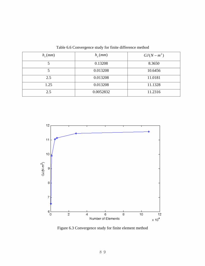
89
Table 6.6 Convergence study for finite difference method
)(mmhx )(mmhy )( 2mNGJ −
5 0.13208 8.3650
5 0.013208 10.6456
2.5 0.013208 11.0181
1.25 0.013208 11.1328
2.5 0.0052832 11.2316
Figure 6.3 Convergence study for finite element method

90
Figure 6.4 Convergence study for finite difference method
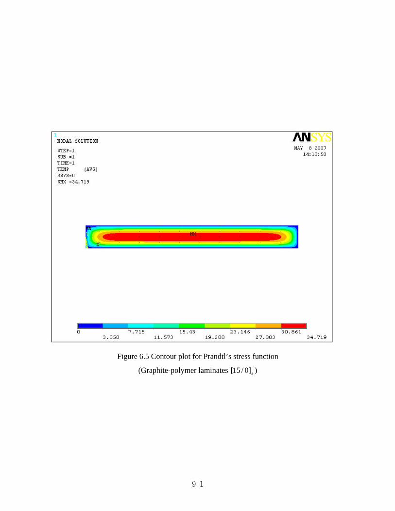
91
Figure 6.5 Contour plot for Prandtl’s stress function
(Graphite-polymer laminates s]0/15[ )
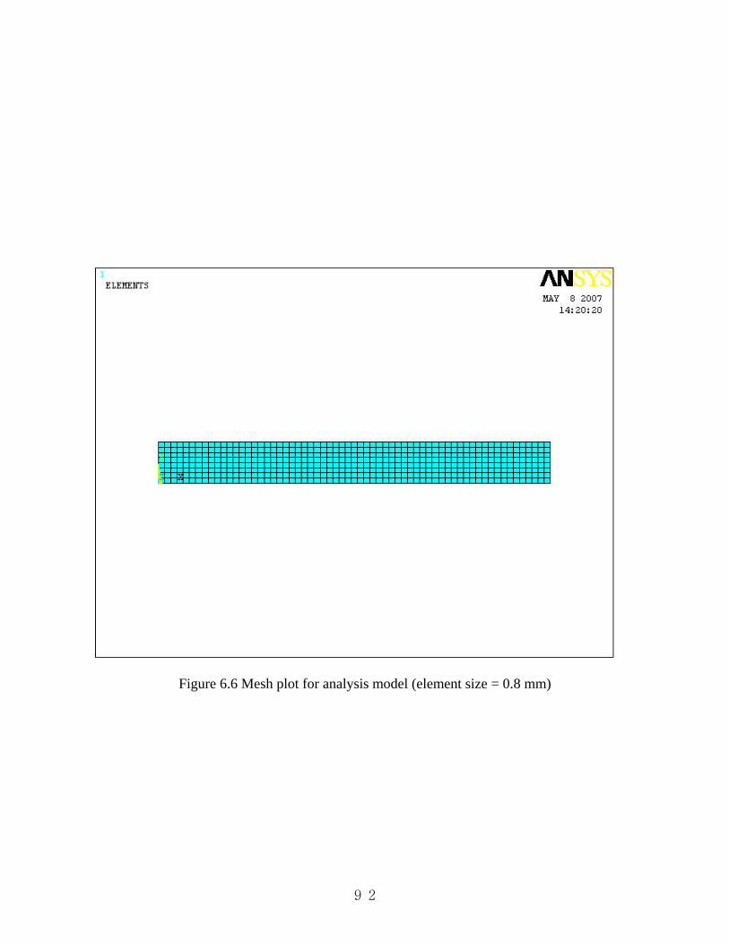
92
Figure 6.6 Mesh plot for analysis model (element size = 0.8 mm)

93
Figure 6.7 Mesh plot for analysis model (element size = 0.5 mm)

94
Figure 6.8 Mesh plot for analysis model (element size = 0.25 mm)
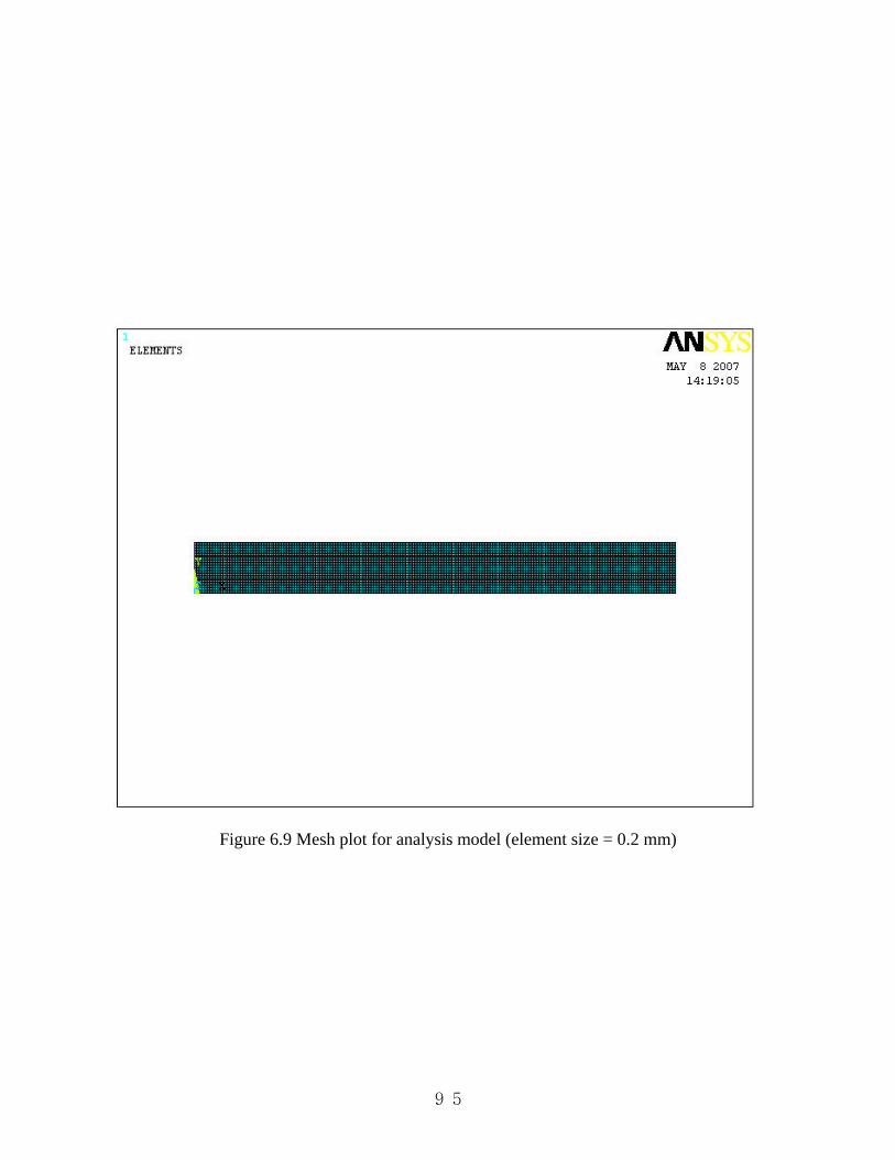
95
Figure 6.9 Mesh plot for analysis model (element size = 0.2 mm)

96
6.2.2 Results and Comparisons
Table 6.5 Comparisons of torsional rigidity of graphite-polymer composite beam
Present ANSYS Finite Difference
Method
Swanson
(1998)
s]0/15[ 15.7015 11.5708 11.2316 11.3498
s]15/30[ 18.3443 16.9941 16.5335 16.8983
s]30/45[ 22.0441 22.9560 22.3845 22.9342
s]60/45[ 21.9371 22.7832 22.2282 22.8769
s]75/60[ 18.1272 16.7771 16.3440 16.7689
s]90/75[ 15.4700 11.4223 11.1083 11.3267
Table 6.6 Comparisons of torsional rigidity of glass-polymer composite beam
Present ANSYS Finite Difference
Method
Swanson
(1998)
s]0/15[ 12.6238 12.2214 11.8625 12.1221
s]15/30[ 15.7472 17.2221 16.7516 17.2311
s]30/45[ 20.9357 22.2895 21.7266 22.3283
s]60/45[ 20.8274 22.1078 21.5631 22.2892
s]75/60[ 15.5597 16.9782 16.5393 16.7829
s]90/75[ 12.4429 12.0434 11.7145 12.1298

97
Table 6.7 Comparisons of torsional rigidity between present analytical method
and ANSYS results
(Graphite-polymer composite)
Present ANSYS Present/ANSYS
s]15/0[ 15.7015 10.2935 1.5254
s]0/15[ 15.7015 11.5708 1.3570
s]30/15[ 18.3443 12.4845 1.4694
s]15/30[ 18.3443 16.9941 1.0795
s]45/30[ 22.0441 18.3550 1.2010
s]30/45[ 22.0441 22.9560 0.9603
s]60/45[ 21.9371 22.7832 0.9629
s]45/60[ 21.9371 18.3223 1.1973
s]75/60[ 18.1272 16.7771 1.0805
s]60/75[ 18.1272 12.3840 1.4638
s]90/75[ 15.4700 11.4223 1.3544
s]75/90[ 15.4700 10.1784 1.5199

98
Table 6.8 Comparisons of torsional rigidity between present analytical method
and ANSYS results
(Glass-polymer composite)
Present ANSYS Present/ANSYS
s]15/0[ 12.6238 10.9747 1.1503
s]0/15[ 12.6238 12.2214 1.0329
s]30/15[ 15.7472 13.0636 1.2054
s]15/30[ 15.7472 17.2221 0.9144
s]45/30[ 20.9357 18.3972 1.1380
s]30/45[ 20.9357 22.2895 0.9393
s]60/45[ 20.8274 22.1078 0.9421
s]45/60[ 20.8274 18.3606 1.1344
s]75/60[ 15.5597 16.9782 0.9165
s]60/75[ 15.5597 12.9450 1.2020
s]90/75[ 12.4429 12.0434 1.0332
s]75/90[ 12.4429 10.8347 1.1484

99
Tables 6.7 and 6.8 show the comparisons of torsional rigidity of laminated composite
between the present analytical approach and finite element results. The results obtained from the
present analytical method seem somewhat strange in that different lay-up sequences of the same
lamina component have the same torsional rigidity. This phenomenon is due to the effective
elastic constants of laminated composites being independent of lay-up sequence. The effective
elastic constants are solely dependent on the components of each lamina of the laminated
composites. From the results obtained from tables 6.7 and 6.8 and the associated shear moduli of
each different angle-ply lamina, one can observe that for the same lamina component but
different lay-up sequence, if the lamina with the higher zxG and lower zyG value lay-up first, the
prediction of torsional rigidity of the laminated composite beam will be more accurate. The
greatest difference between the finite element results and the present analytical results are 52.5%
and 20.5% for graphite-polymer composite and glass-polymer composites, respectively. If the
lamina lay-up order uses the lamina with higher zxG and lower zyG value places in the outer layer,
the greatest difference between the finite element results and present analytical method will
decrease to 35.7% and 8.56% for graphite-polymer and glass-polymer composites, respectively.

100
Chapter 7 Summary and Conclusions
The primary objective of this study is to analytically investigate the torsional rigidity of
laminated composite beams and compare the results with those from the finite element method,
finite difference method, and a previous paper (Swanson, 1998). Torsion of cylindrical shafts has
long been a basic subject in classical theory of elasticity. In the first chapter, many previous
works about the torsional problem were being discussed. All of the previous works formulated
the torsion problem by following the classical approach, which was proposed by Saint Venant.
For some simple geometrical shapes, analytical solutions are readily available. For other more
complex geometry, numerical methods, such as the finite element or finite difference method, are
usually utilized to obtain the solution.
The analytical method proposed here utilized the concept of the effective elastic constant of
laminated composite materials. The formulation of the effective elastic constant of laminated
composites has been proposed by many previous researchers. This study primarily adopts the
formulation from Chou et al. (1971). From that approach, a layered medium with monoclinic
anisotropy is considered. Within these laminated composites, the conditions of uniform strain in
the layering direction and constant stress in the direction normal to layering are assumed. After a
long mathematical derivation, the non-homogeneous anisotropic laminated composite is
transformed into an equivalent homogeneous anisotropic material. The obtained effective shear
moduli of the homogenized material can then be used to determine the effective torsional rigidity
of the laminated composite rods by the theory developed by Lekhnitskii (1963).
The classical formulation of the torsion problem of composite laminates is presented in
chapter 3. A theoretical solution for the torsion problem of laminated composites is presented.
Two continuity conditions have to be satisfied between the interfaces of each layer. The partial
derivative of the stress function with respect to x must be equal between two neighboring layers,
and the partial derivative of the stress function with respect to y times the reciprocal of the shear
modulus in the x-z direction must be constant within each layer. The outer boundary conditions
are set to be stress free as in the classical formulation. Finally, the eigenfunction expansion
method is employed to solve the formulated problem.
Two numerical methods are employed in this study, the finite element method and the
finite difference method. In the finite element method, the finite element commercial package

101
ANSYS 9.0 is used to model the laminated composite beam problem. In the finite difference
method, the finite difference codes are developed to analyze the torsional problem of laminated
composite rods. In order to show the effectiveness and accuracy of both numerical methods,
three verification examples with different material properties and geometrical dimensions are
used in the validation stage.
A total of twenty-four analysis models composed of different ply-angle layers are created
and analyzed in this study. Two commonly used composite materials (Graphite-polymer and
Glass-polymer composites) are used to build the analysis model. The dimensional parameters of
the analysis models are used from previous work (Swanson, 1998), and the material properties of
each lamina are from a composites book (Hyer, 1998).
The finite element models and finite difference models developed in this study are capable
of predicting the torsional rigidity of laminated composite rods. Good agreement was found
between the finite element method, finite difference method, and previous results (Swanson,
1998). From the results in chapter 6, one can see that the present analytical method doesn’t
predict very well for the torsional rigidity compared with the previous work and both numerical
methods. The reason behind the difference is that the first stage of the present analytical method
employed the idea of effective elastic constants instead of the classical Saint Venant approach.
The formulation of effective elastic constant considers a three dimensional layered medium. The
deformation mode of this typical laminate is assumed as constant stress in the direction normal to
layering and uniform strain in the layering direction. Both these assumptions will be violated
when the laminated composite is subjected to torsional loading. Hence, the concept of effective
elastic constants is not suitable in the prediction of the torsional rigidity of laminated composite
rods.
102
REFERENCES
Achenbach, J. D., “The Layered Medium as a Homogeneous Continuum with Microstructure,” AFML-TR-70-275, 1970. Argyris, J. H. and Kelsey, S., “Energy Theorems and Structural Analysis,” Butterworth Scientific Publications, London, 1960. ANSYS, “Documentation and Theory Reference,” Version 9.0, ANSYS, Inc., 2004. Behrens, E., “Sound Propagation in Lamellar Composite Materials and Averaged Elastic Constants,” Journal of the Acoustical Society of America, Vol. 42, 1967, pp. 378-383. Booker, J. R. and Kitipornchai, S., “Torsion of Multilayered Rectangular Section,” Journal of the Engineering Mechanics Division, ASCE, 1971, pp. 1451-1468. Boresi, A. P. and Schmidt, R. J., “Advanced Mechanics of Materials,” Sixth edition, John Wiley & Sons, Inc., 2003. Boresi, A. P., Chong, K. P. and Saigal, S., “Approximate Solution Methods in Engineering Mechanics,” Second Edition, John Wiley & Sons, Inc., 2003. Cheng, S., Wei, X. and Jiang, T., “Stress Distribution and Deformation of Adhesive Bonded Laminated Composite Beams,” Journal of Engineering Mechanics, ASCE, Vol. 115, 1989, pp. 1150-1162. Chou, P. C., Carleone, J. and Hsu, C. M., “Elastic Constants of Layered Media,” Journal of Composite Materials, Vol. 6, 1972, pp.80-93. Chou, P. C. and Wang, A. S. D., “Control Volume Analysis of Elastic Wave Front in Composite Materials,” Journal of Composite Materials, Vol. 4, 1970, pp. 444-453. Clough, R. W., “The Finite Element Method in Plane Stress Analysis,” Journal of the Structures Division, ASCE, Proceedings of the second Conference on Electronic Computation, 1960, pp. 345-378. Courant, R., “Variational Methods for the Solution of Problems of Equilibrium and Vibration,” Bulletin of the American Mathematical Society, Vol. 49, 1943, pp. 1-43. Davalos, J. F., Qiao, P., Wang, J., Salim, H. A. and Schlussel, J., “Shear Moduli of Structural Composites from Torsion Tests,” Journal of Composite Materials, Vol. 36, 2002, pp. 1151-1173. Ely, J. F. and Zienkiewicz, O. C., “Torsion of Compound Bars: a Relaxation Solution,” International Journal of Mechanical Sciences, Vol. 14, 1960, pp. 356-365.

103
Enie, R. B. and Rizzo, R. R., “Three-Dimensional Laminate Moduli,” Journal of Composite Materials, Vol. 4, 1970, pp. 150-154. Friedman, Z. and Kosmatka, J. B., “Torsion and Flexure of A Prismatic Isotropic Beam Using the Boundary Element Method,” Computers and Structures, Vol. 74, 2000, pp. 479-494. Hashin, Z. and Shtrikman, S., “A Variational Approach to the Theory of the Elastic Behavior of Multiphase Materials,” Journal of the Mechanics and Physics of Solids, Vol. 11, 1963, pp. 127-140. Herrmann, R. L., “Elastic Torsional Analysis of Irregular Shapes,” Journal of Engineering Mechanics Division, ASCE , Vol. 9, 1965, pp. 11-19. Hrenikoff, A., “Solution of Problems in Elasticity by the Framework Method,” Journal of Applied Mechanics, Vol. 8, 1941, pp. 169-175. Hyer, M. W., “Stress Analysis of Fiber-Reinforced Composite Materials,” McGraw-Hill, 1998. Jawson, M. A. and Ponter, R. A., “An Integral Equation Solution of the Torsion Problem,” Proceedings of the Royal Society London, Vol. 275, 1963, pp. 237-246. Karayannis, C. G., “A Numerical Approach to Steel Fiber Reinforced Concrete under Torsion,” Structural Engineering Review, Vol. 7, 1995, pp. 83-91. Lekhnitskii, S. G., “Theory of Elasticity of an Anisotropic Elastic Body,” MIR Publishers, Moscow, 1963. Li, Z., Ko, J. M. and Ni, Y. Q., “Torsional Rigidity of Reinforced Concrete Bars with Arbitrary Sectional Shape,” Finite Elements in Analysis and Design, Vol. 39, 2000, pp. 349-361. Muskhelishvili, N. I., “Some Basic Problems of the Mathematical Theory of Elasticity,” Noordhoff, Groningen, 1963. Packham, B. A. and Shail, R., “St. Venant Torsion of Composite Cylinders,” Journal of Elasticity, Vol. 8, 1978, pp. 393-407. Pagano, N. J., “Exact Moduli of Anisotropic Laminates,” in Composite Materials, Broutman, L. J. and Krock, R. H., eds., Vol. 2, Mechanics of Composite Materials, Sendeckyj, G. P., ed., Academic Press, 1974, pp. 23-45. Postma, G. W., “Wave Propagation in a Stratified Medium,” Geophysics, Vol. 20, 1955, pp. 780-806. Reddy, J. N., “An Introduction to the Finite Element Method,” McGraw-Hill, 2006. Saada, A. S., “Elasticity: Theory and Applications,” Krieger Publishing Company, 1993.

104
Salamon, M. D. G., “Elastic Moduli of a Stratified Rock Mass,” International Journal of Rock Mechanics and Mining Sciences, 1968, pp. 519-527. Sapountzakis, E. J., “Nonuniform Torsion of Multi-material Composite Bars by the Boundary Element Method,” Computers and Structures, Vol. 79, 2001, pp. 2805-2816. Sapountzakis, E. J. and Mokos, V. G., “Nonuniform Torsion of Composite Bars by Boundary Element Method,” Journal of Engineering Mechanics, 2001, pp. 945-953. Sapountzakis, E. J. and Mokos, V. G., “Warping Shear Stresses in Nonuniform Torsion of Composite Bars by BEM,” Computational Methods in Applied Mechanics and Engineering, Vol. 192, 2003, pp. 4337-4353. Savoia, M. and Tullini, N., “Torsional Response of Inhomogeneous and Multilayered Composite Beams,” Composite Structures, Vol. 25, 1993, pp. 587-594. Sun, C. T., Achenbach, J. D. and Herrmann, G., “Continuum Theory for a Laminated Medium,” Journal of Applied Mechanics, Vol. 35, 1968, pp. 467-480. Sun, C. T. and Li, S., “Three-Dimensional Effective Elastic Constants for Thick Laminates,” Journal of Composite Materials, Vol. 22, 1988, pp. 629-639. Swanson, S. R., “Torsion of Laminated Rectangular Rods,” Composite Structures, Vol. 42, 1998, pp. 23-31. Timoshenko, S. P. and Goodier, J. N., “Theory of Elasticity,” New York, McGraw-Hill, 1970. Tsai, C. L., Daniel, I. M. and Yaniv, G., “Torsional Response of Rectangular Composite Laminates,” Journal of Applied Mechanics, Vol. 57, 1990, pp. 383-387. Turner, M., Clough, R. W., Martin, H. H., and Topp, L., “Stiffness and Deflection Analysis of Complex Structures,” Journal of Aeronautical Sciences, Vol. 23, 1956, pp. 805-823. Ugural, A. C. and Fenster, S. K., “Advanced Strength and Applied Elasticity,” Fourth edition, Prentice Hall, 2003. White, J. E. and Angona, F. A., “Elastic Wave Velocities in Laminated Media,” Journal of the Acoustical Society of America, Vol. 27, 1955, pp. 310-317. Zhang, J. and Li, S., “Torsion of Composite Laminated Bars with a Large Number of Layers,” Applied Mathematics and Mechanics, Vol. 19, 1998, pp. 585-591.

105
Vita Kunlin Hsieh was born in Kaohsiung, Taiwan on December 3, 1978 to Wei Jui and Joneming
Hsieh. He is the middle of three children. In 1999 Kunlin Hsieh graduated from National
Kaohsiung University of Applied Sciences, where he obtained his Associate Degree in Civil
Engineering. He graduated from Tamkang University at Taipei, where he obtained his Bachelor
of Science Degree in Construction Engineering in June 2001. In the fall of 2004, he joined
Department of Engineering Science and Mechanics at Virginia Polytechnic Institute and State
University to continue an academic career towards a Master’s Degree in Engineering Mechanics.
Kunlin Hsieh proudly received the degree of Master of Science in Engineering Mechanics in
May 3, 2007.