numerical methods with python - florida...

Numerical Methods with Python

1 Introduction

You will be given light curve data for several RR Lyrae variables. This datawill be processed to find the periods and flux averaged magnitudes of thestars.

2 Objectives

1. Plot the raw light curves.

2. Find the periods in the light curves.

3. Phase the light curves.

4. Fit a Fourier series to the light curves.

5. Fit the light curves to a template.

6. Integrate the light curves to find the flux averaged magnitude.

3 Plotting the Data

The data will be provided in a text file with each line containing (in thisorder) the time (in mean Julian date), brightness (apparent magnitude), anderror in brightness of the star. Plot the brightness as a function of time. Bylooking at this plot, what can you tell about the behavior of the brightnessas a function of time, if you can tell anything at all?

4 Finding the Periods in the Data

Fourier analysis (described in chapter 5 of the appendix) can be used toextract the period(s) from a set of irregularly and/or sparsely sampled pe-riodic data. Instead of writing the code in python to do this yourself, youcan use a mainstream astronomy tool, Period04.

Download the free tool Period04:

http://www.univie.ac.at/tops/Period04/

1

Be sure to also download the Period04 manual and the tutorial data files.Go through both tutorials in the manual.

After you have gone through these tutorials, you should be able to ex-tract the dominant periods from the data. Record and report these periodsfor each data set; you will need them later. Also show and describe a peri-odogram.

For reference, typical RR Lyrae periods range from a few hours to 1.5days.

In the event Period04 fails to work properly, then try Supersmoother.The instructor should provide you this code.

5 Phasing the Data

Phasing the data is also referred to as period folding.Data cannot be taken continuously (data can only be taken at night,

other people have to use the telescope, etc.) nor can it necessarily be takenat the same rate (some nights may have more data than others). The periodof the observed star may be less than the period of data taking. Therefore,each night of data taking may sample a different portion of the star’s cycle.The objective of period folding is to take observations spanning many cyclesand condense them to one cycle.

Since the periods are known, the data can be folded to any period P .Suppose the first datum occurs at time t0. Then, to phase the data at timet ≥ t0, the time difference is divided by the period: (t − t0)/P . However,since we want 0 ≤ P ≤ 1 and the data is periodic, the integral portion ofthe ratio is subtracted to find where the datum at time t lies (given by thephase Φ) within one period:

Φ =t− t0P− int

(t− t0P

).

A video explanation of period folding can be found at the University ofNorth Carolina’s website:

http://skynet.unc.edu/ASTR101L/videos/folding/

Fold the light curves into their primary period(s) and plot the phaseddata.

2

6 Fitting a Fourier Series to the Data

We want to fit the light curves to a Fourier series such that we have a con-tinuous expression for the light curve. Fit the data to a nine-term Fourierseries using a χ2 minimization process. This is rigorously explained in chap-ter 3, particularly section 3.6, of the appendix. The form of the Fourierseries follows:

m(t) = 〈m〉+9∑

k=1

Ak sin (2πkft+ φk)

where m(t) is the observed brightness, 〈m〉 is the mean brightness, Ak isthe amplitude of the kth harmonic of the Fourier series, f = 1/P is thefrequency where P is the fitted period of the magnitude variation, and φkis the phase of the kth harmonic at t = 0. The parameters to be fit here areAk and φk.

Fit the light curves to Fourier series and report the results.Hint: If the data and its error are given by vi and σi, respectively:

χ2 =∑i

(m− viσi

)2

7 Fitting a Template to the Data

Templates are sets of data points corresponding to the expected shape of alight curve. Often, stars can be categorized by a finite and small number oftemplates, and the best fit template of a light curve can reveal the type ofstar for which the light curve is taken.

You will be given a number of templates. Fit these templates to theperiod-folded data using a χ2 minimization procedure and see which tem-plate fits best. Interpolation (which can be performed by python) will berequired, as the templates are not guaranteed (and, in general, do not) havepoints at the same times as you have data. Furthermore, the amplitudesand means of the templates will have to be adjusted in order to fit the data.

8 Integrating the Light Curve

In astronomy, the brightness of a star is generally given by apparent mag-nitude m, and luminosity is generally given by absolute magnitude M such

3

that for a star a distance d away, the flux F is given by

F =M

4πd2.

Most RR Lyrae stars have M = 0.6. Knowing this, the distance d can befound in parsecs:

m−M = −5 + 5 log10 d.

The flux averaged magnitude FAM is given by the integral of the flux inphase space:

FAM = −2.5

∫ 1

0F (Φ)dΦ

The flux averaged magnitude is used in various physical analyses of stellarprocesses.

Integrate the phased light curves and report the values.

4

9 Appendix

5

34 Chapter 3. The method of least squares

Table 3.1: Observations of the periods, P (days), the absolute magnitude M, and the colour B − V ,of Cepheids in the LMC.

log P M B-V log P M B-V log P M B-V

0.408 -2.39 0.58 0.978 -4.81 0.84 1.367 -5.18 0.900.429 -2.53 0.51 0.993 -4.10 0.69 1.388 -5.50 0.710.492 -3.38 0.53 1.038 -4.28 0.75 1.425 -5.01 1.040.529 -2.72 0.60 1.051 -4.05 0.76 1.453 -5.15 0.900.569 -2.95 0.58 1.119 -4.23 0.85 1.484 -5.80 0.770.677 -3.32 0.64 1.134 -4.58 0.75 1.503 -5.33 0.930.703 -3.45 0.61 1.160 -4.40 0.85 1.536 -5.23 0.810.841 -3.81 0.66 1.209 -5.05 0.72 1.563 -6.11 0.830.911 -3.90 0.73 1.272 -4.79 0.82 1.655 -5.34 1.200.936 -4.11 0.72 1.303 -4.76 0.86 1.684 -6.13 0.960.960 -4.24 0.57 1.353 -4.65 0.98 1.897 -6.45 1.24

εi = a0 + a1xi − yi

ε2i = (a0 + a1 xi − yi)2

S =n∑

i=1ε2i =

n∑

i=1(a0 + a1 xi − yi)2

where n is the number of observations. Our problem is to minimize S with respect to a0 and a1. Tominimize with respect to a0 we find ∂S/∂a0 and set it to zero, and we do the same for a1:

∂S∂a0

= 2n∑

i=1(a0 + a1 xi − yi) = 0

∂S∂a1

= 2n∑

i=1(a0 + a1 xi − yi)xi = 0

Thereforen∑

i=1(a0 + a1 xi − yi) = 0

n∑

i=1(a0 xi + a1 x2

i − xiyi) = 0

We can re-write these two equations as follows

na0 + a1

n∑

i=1xi −

n∑

i=1yi = 0

a0

n∑

i=1xi + a1

n∑

i=1x2

i −n∑

i=1xiyi = 0

3.1. Linear least squares 35

-6.5

-6

-5.5

-5

-4.5

-4

-3.5

-3

-2.5 0.4 0.6 0.8 1 1.2 1.4 1.6 1.8 2

M

log(P)

Figure 3.1: The relationship between the absolute magnitude, M, and the logarithm of the period(days), log P, for Cepheids in the LMC (from Table 3.1). The solid line is the least-squares fit whenlog P is error free; the dashed line is the least-squares fit when M is error free.

From the data in Table 3.1 we can clearly determine the sums∑ xi,

∑ yi,∑ xiyi and

∑ x2i . Therefore

the values of a0 and a1 can be found because we have two equations in two unknowns.The above notation is clumsy, so let us represent the average of any quantity as follows:

< x >= 1n

n∑

i=1xi

which allows us to write the above equations as

a0 + a1 < x > = < y >a0 < x > +a1 < x2 > = < xy >

In matrix notation we can write these two simultaneous equations as( 1 < x >< x > < x2 >

) ( a0a1

)=

(< y >< xy >

).

or more simply asXA = Y

from which the unknown coefficient matrix, A, can be obtained:

A = (X−1)Y.

where X−1 is the inverse of the matrix X. In this simple case we do not need direct matrix inversionand algebraic manipulation easily leads to the solution

a1 =< xy > − < x >< y >< x2 > − < x >2

a0 = < y > −a1 < x >


Applying these equations to our problem of Cepheid variables, we find M = −2.547 log P − 1.619(solid line in Fig. 3.1) . Given the observed values of log Pi and Mi in Table 3.1, we can calculate

σ2 =1n

n∑

i=1ε2i =

1n

n∑

i=1(a0 + a1 log Pi − Mi)2

using a0 = −1.619, a1 = −2.547, from which we can determine the standard deviation, σ, of the fitto the straight line. This turns out to be σ = 0.28 mag. Therefore we can state that the equationM = −2.547 log P− 1.619 allows the absolute magnitude, M, of any Cepheid with known period tobe determined with a standard deviation of 0.28 mag.

Now, we chose to assume on reasonable grounds that all the error resides in the absolute mag-nitude, M (the y value) and that log P (the x value) is free of error. If we had, instead, assumed thatall the error can be attributed to log P, we will obtain different results. Re-writing the equation aslog P = 1

a1M − a0

a1and repeating the calculations gives a1 = −2.745, a0 = −1.397. This is quite

different (dashed line in Fig. 3.1), emphasizing that we need to think carefully in such matters.In the first case we minimized the errors in y, assuming that the errors in x were negligible

compared to those in y. In the second case we minimized the errors in x, assuming that the errors iny were negligible compared to those in x. What do we do if the errors in x are comparable to thosein y? This problem is beyond the scope of this course, but it will clearly lead to values of a0 and a1which lie somewhere between the two cases we have considered.

Exercises3.1.1 Write a program which reads the data of Table 3.1 from a file and calculates the linear least-

squares coefficients a0 and a1 in M = a0 + a1 log P. Plot the data points and the straight linethus calculated. [Answer: a0 = −1.619033, a1 = −2.547323.]

3.2 χ2 minimizationIn the above discussion we assumed that the errors in the straight line fit belong to a single normaldistribution with standard deviation σ. What happens if the errors belong to different normal distri-butions with different values of σ? This may happen if, for example, if the data were obtained withinstruments of different precisions, then some points deserve more weight than others. In cases likethese, we minimize χ2 where

χ2 =n∑

i=1

(y − yiσi

)2.

Here yi is the variable subject to errors, y = a0 + a1xi is the function whose coefficients are required(xi assumed to be free of error) and σi is the standard deviation of data point i. Least squares fittingis just a special case of χ2 minimization with σi = σ = a constant.

Our problem is to minimize χ2 with respect to a0 and a1 for

χ2 =n∑

i=1

(a0 + a1 xi − yi

σi

)2.

Equating the partial differentials with respect to a0 and a1 to zero, we obtain the result

∆ =∑

1/σ2∑

x2/σ2 −(∑

x/σ2)2

a0 =(∑

y/σ2∑

x2/σ2 −∑

x/σ2∑

xy/σ2)/∆

a1 =(∑

1/σ2∑

xy/σ2 −∑

x/σ2∑

y/σ2)/∆

When σ2i = σ

2 = constant, we recover the least squares result.

3.3. Uncertainties in the coefficients 37

Exercises

3.2.1 Derive the equations for a0 and a1 using χ2 minimization of yi + εi = a0 + a1 xi given thestandard deviations σi for each of the n data points.

3.2.2 Write a program to calculate the χ2 estimates of a0 and a1. Test your program by reading thedata of Table 3.1 and setting σi = log Pi. [Answer a0 = −1.511525 and a1 = −2.651885].

3.3 Uncertainties in the coefficients

The uncertainites in the coefficients a0 and a1 are quite easy to do derive, but rather tedious. First,we note that the errors in the coefficients depend only on the errors in y (if the y i were free of errorthere would be no errors in the coefficients). This is a problem in propagation of errors - we want toknow how the standard deviation of a0 and a1 depend on yi. Therefore

σ2a0 =

(∂a0∂y1

)2σ2

1 +

(∂a0∂y2

)2σ2

2 + . . . +

(∂a0∂yn

)2σ2

n =

n∑

i=1

(∂a0∂yi

)2σ2

i

and in the same way

σ2a1 =

n∑

i=1

(∂a1∂yi

)2σ2

i

so we need partial derivatives with respect to each individual point, y i. These are

∂a0∂yi

=(1/σ2

i

∑x2/σ2 − xi/σ

2i

∑x/σ2

)/∆

(∂a0∂yi

)2σ2

i =1/σ2

i(∑ x2/σ2

)2 − 2xi/σ2i∑ x2/σ2 ∑ x/σ2 + x2

i /σ2i(∑ x/σ2

)2

∆2

n∑

i=0

(∂a0∂yi

)2σ2

i =

∑1/σ2

(∑ x2/σ2)2 − 2

∑ x/σ2 ∑ x2/σ2 ∑ x/σ2 +∑ x2/σ2

(∑ x/σ2)2

∆2

=

∑1/σ2

(∑ x2/σ2)2 −∑ x2/σ2

(∑ x/σ2)2

∆2 =

∑ x2/σ2

∆∂a1∂yi

=(xi/σ

2i

∑1/σ2 − 1/σ2

∑x/σ2

)/∆

(∂a1∂yi

)2σ2

i =x2

i /σ2i(∑ 1/σ2

)2 − 2xi/σ2i(∑ 1/σ2

) (∑ x/σ2)+ 1/σ2

(∑ x/σ2)2

∆2

n∑

i=1

(∂a1∂yi

)2σ2

i =

∑ x2/σ2(∑ 1/σ2

)2 − 2 ∑ x/σ2(∑ 1/σ2

) (∑ x/σ2)+

∑ 1/σ2(∑ x/σ2

)2

∆2

=

∑ x2/σ2(∑ 1/σ2

)2 −(∑ 1/σ2

) (∑ x/σ2)2

∆2 =

∑ 1/σ2

∆

So we finally obtain σ2a0 =

∑ x2/σ2/∆ and σ2a1 =

∑ 1/σ2/∆with ∆ = ∑ 1/σ2 ∑ x2/σ2−(∑ x/σ2

)2.


Exercises3.3.1 Modify the program in Ex. 3.2.2 to calculate and print the standard deviations of a0 and a1.

Test your program by reading the data of Table 3.1 and setting σi = 0.1 × log Pi. [Answera0 = −1.511525, σa0 = 0.034749, a1 = −2.651885, σa1 = 0.040433.]

3.4 Multivariate least squaresIn the last section we saw how we could obtain best estimates of the coefficients involving only twovariables, x and y. It is sometimes the case that we have functional relationships involving more thantwo variables. Expanding on the example of the pulsating Cepheid stars, it can be shown that theperiod - luminosity law ought to depend somewhat on the temperature of the star. In other words,one should be able to obtain a more accurate absolute magnitude, M, (and thus a more accuratedistance) if the temperature of each Cepheid is included in the relationship. The temperatures ofstars are measured by the ratio of the brightness through blue and red filters. This ratio expressed inmagnitudes is called B − V . Hence we may expect a relationship of the form

M = a0 + a1 log P + a2(B − V)

where, as before, the coefficients a0, a1, a2 can be determined using the method of least squares. Letus see if we can apply the same technique to the general relationship yi + εi = a0 + a1x1i + a2 x2i,where we have written Mi = yi, log Pi = x1i and (B − V)i = x2i. Note that we assume (B − V) to befree of error (which is not strictly true). We have

εi = a0 + a1 x1i + a2 x2i − yi

ε2i = (a0 + a1 x1i + a2 x2i − yi)2

S =n∑

i=1ε2i =

∑(a0 + a1x1i + a2 x2i − yi)2

Minimizing S with respect to a0, a1, a2

∂S∂a0

= 2∑

(a0 + a1 x1i + a2x2i − yi)

∂S∂a1

= 2∑

(a0 + a1 x1i + a2x2i − yi)x1i

∂S∂a2

= 2∑

(a0 + a1 x1i + a2x2i − yi)x2i

Equating these to zero, you can see that we obtain three equations in the three unknowns, a0, a1, a2:

a0 + a1 < x1 > +a2 < x2 > = < y >a0 < x1 > +a1 < x2

1 > +a2 < x1x2 > = < x1y >a0 < x2 > +a1 < x1x2 > +a2 < x2

2 > = < x2y >

This time the simple algebraic solution is more laborious and it is best to use matrix methods. Theabove system of equations is written as

1 < x1 > < x2 >

< x1 > < x21 > < x1x2 >

< x2 > < x1x2 > < x22 >

a0a1a2

=< y >< x1y >< x2y >

,

3.4. Multivariate least squares 39

or XA = Y. The matrix of unknown coefficients, A, is obtained by finding the inverse of X, so thatA = (X−1)Y.Matrix inversion is one of the most important numerical techniques. In python, matrixarithmetic, including matrix inversion, is available by importing the numpy module as explained inChapter 1.

How would we program this in python? Actually, we may as well expand further and generalizethe problem to the model

yi + εi = a0 + a1 x1i + a2 x2i + a3 x3i + ... + am xmi

which means that the linear equation of the previous section is a special case with m = 1, while thecase described above has m = 2. m is therefore the number of independent variables. Our programneeds to construct two matrices, X and Y:

X =

1 < x1 > < x2 > ... < xm >< x1 > < x2

1 > < x1 x2 > ... < x1xm >< x2 > < x1x2 > < x2

2 > ... < x2xm >... ... ... ... ...

< xm > < x1 xm > < x2xm > ... < xmxm >

, Y =

< y >< x1y >< x2y >...

< xmy >

.

Since we will be dealing with arrays and matrices, we must import the numpy module. Here is thefull least squares program.

1 from numpy import *

2

3 # Multivariate least squares fit y = a0 + a1*x1 + a2*x2 + ... + am*xm

4

5 m = int(raw_input("Number of independent variables? "))

6 m1 = m + 1

7 fp = open("mlstsq.dat","r")

8 x = zeros((m1,m1))

9 y = zeros((m1,1))

10 xi = [0.0]*m1

11 n = 0

12 for line in fp:

13 xi[0] = 1.0

14 for j in range(1,m1):

15 xi[j] = float(line.split()[j-1])

16 yi = float(line.split()[m])

17 for j in range(m1):

18 for k in range(m1):

19 x[j,k] += xi[j]*xi[k]

20 y[j,0] += yi*xi[j]

21 n += 1

22 fp.close()

23 X = mat( x.copy() )

24 Y = mat( y.copy() )

25 A = X.I*Y

26 for j in range(m1):

27 print "A[%d] = %f" % (j, A[j])


Let’s examine this program. In line 1 we import the numpymodule for the reason mentioned above.In line 5 we ask the user to type in the number of independent variables. This is 1 for y = a0 + a1 x1,2 for y = a0 + a1 x1 + a2 x2, etc. Note that the matrix X has dimension m1× m1 where m1 is one morethan the number of independent variables, m. In line 7 we open the input file for reading and in line22 we close it after we have read all the data. In line 8 we define x to be an m1 × m1 array and weset all its elements to zero using the zeros statement. Remember that the Y matrix is a row matrixwith m1 rows and one column. In line 9 we define the y array and set the array elements to zero.We will be using the x and y arrays to hold the running total as we loop through the data. In line10 we define xi to be a list of zeros of size m1. The xi list will be used for reading the numbers,xi1, xi2, ..., xim from each line of the file. The variable yi will hold yi which is the last number oneach line.

From line 12 to line 21 we read and operate on each line of the file as it is read, using n to countthe number of lines (i.e. the number of data points). We set xi[0] = 1 because we need not onlyproducts such as < x1 x2 >, but also < x1 >=< 1× x1 >=< x0x1 > . In line 15 we store each numberin the line to the corresponding value of xi. In line 16 we store the last number in the line (the y ivalue) to yi. In lines 18 and 19 we form the products xi j xik and add the result to the running totalin array x[j,k]. In line 20 we add the product yi xi j to the running total y[j,0].

By the time we reach line 22 we have read all the lines in the file and we have these sums inarrays x and y as follows:

x[j, k] =n∑

i=1xi j xik j,k = 0,1,2, ..., m

y[j, 0] =n∑

i=1xi jyi j = 0,1,2, ..., m

These are just n times the required averages, < x jxk >, < x jy >, but since we will be dividing byn after matrix inversion, there is really no need to divide these arrays by n. In lines 23 and 24 weconvert the arrays to the corresponding matrices which then allows us to form the inverse of matrixX and multiply it by matrix Y to get the matrix of coefficients, A. The coefficients are our finalanswers which we print out in a loop (lines 26 and 27).

Applying this method to our Cepheid problem, we obtain the following coefficients:

M = −2.145 − 3.117 log P + 1.486(B − V)

with a residual standard deviation of σ = 0.25 mag in M. This is certainly a useful improvementover the simple linear relationship (σ = 0.28 mag) discussed in the previous section.

Exercises3.4.1 Use the above program to calculate the linear least-squares coefficients in M = a0+a1 log P+

a2(B−V) using the data of Table 3.1. [Answer: a0 = −2.1452, a1 = −3.1173, a2 = 1.4857.]

3.5 Fitting a polynomialIt often happens that simple linear relationship of the form yi = a0+a1xi is not a good representationof the data and that it is best represented by a polynomial of degree m, i.e.

yi + εi = a0 + a1 xi + a2 x2i + a3x3

i + ... + amxmi .

This is just another example of the multivariate case described above. In the case of a quadratic,y = a0 + a1 x + a2 x2, we can simply put x1 = x, x2 = x2 and use the above program to obtain thecoefficients. For the general polynomial we just put xi = xi.

3.6. Fourier fitting 41

Exercises3.5.1 The following program generates a cubic polynomial with coefficients in list a and with

simulated observational errors:

import random

fp = open("polynomial.dat","w")

a = [1.0, -2.0, 3.0, -4.0] # Change the coefficients as desired.

n = 100 # Number of data points.

for i in range(n):

x = 0.01*i # Value of x.

y = a[0]

for j in range(1,4):

y += a[j]*x**j # Value of y.

# Mess up y by adding some noise with standard deviation 0.1.

y += random.gauss(0.0,0.1)

fp.write("%8.3f %10.3f\n" % (x,y))

fp.close()

Use this program to generate (x, y) data in file polynomial.dat. Modify the general least-squares program discussed in the previous section to read this file and to fit a polynomial ofany given degree. Test your program by comparing the resulting coefficients with those usedto generate the file. The values will not be identical because of the added scatter.

3.6 Fourier fittingThere are many other uses for least squares. One of the most interesting is for Fourier fitting. Anyperiodic function can be described by a sum of Fourier components of the form

Y = a0 + A1 sin(ωt + φ1) + A2 sin(2ωt + φ2) + A3 sin(3ωt + φ3) + ... + Am sin(mωt + φm)

where ω = 2π/P, P is the period, φ is the phase in radians and a0, A1, ..., Am, φ1, ..., φm are unknowncoefficients. We can write this more compactly in the form

Y = a0 +m∑

k=1Ak sin(kωt + φk)

= a0 +m∑

k=1(Ak cos φk sin(kωt) + Ak sin φk cos(kωt))

= a0 +m∑

k=1(a2k−1 sin(kωt) + a2k cos(kωt))

So finally we have

Y = a0 + a1 sin(ωt) + a2 cos(ωt) + a3 sin(2ωt) + a4 cos(2ωt) + ... + a2m−1 sin(mωt) + a2m cos(mωt).

Suppose we have some periodic data, it could be for example the light curve of a Cepheid.We are given the time, ti, and magnitude, yi, of an observation and we have n such observations.We know the period, P, and therefore ω = 2π/P. For any given observation we can put x1i =sin(ωti), x2i = cos(ωti), x3i = sin(2ωti), x4i = cos(2ωti), ..., etc. As you can see, this is the samekind of problem as before,

Yi = yi + εi = a0 + a1 x1i + a2 x2i + a3 x3i + ... + a2m−1 x(2m−1)i + a2m x2mi,


and we use least squares to determine the unknown coefficients, ak. The python program is shownbelow.

#

# Program to fit a time series with Fourier components.

#

from numpy import *

import math

per = float(raw_input("Period? "))

w = 2.0*math.pi/per

nf = int(raw_input("Number of Fourier components? "))

fp = open("fourier.dat","r")

# m1 is the number of unknown coefficients.

m1 = 2*nf + 1

# Create empty matrices.

x = zeros((m1,m1))

y = zeros((m1,1))

xi = [0.0]*m1

n = 0

#

# Read (time, value) from each line of the file.

for line in fp:

t = float(line.split()[0])

yi = float(line.split()[1])

xi[0] = 1.0

for k in range(1,nf+1):

xi[2*k-1] = math.sin(k*w*t)

xi[2*k] = math.cos(k*w*t)

for j in range(m1):

for k in range(m1):

x[j,k] += xi[j]*xi[k]

y[j,0] += yi*xi[j]

n += 1

fp.close()

# Copy to big matrices.

X = mat( x.copy() )

Y = mat( y.copy() )

# Invert X and multiply by Y to get coefficients.

A = X.I*Y

# Solution is A0 + Sum[ Amp*sin(k*wt + phi) ]

print "a[0] = %f" % A[0]


amp = math.sqrt(A[2*k-1]**2 + A[2*k]**2)

phs = math.atan2(A[2*k],A[2*k-1])

print "amp[%d] = %f phi = %f" % (k, amp, phs)

3.7. Non-linear least squares 43

Exercises3.6.1 Write a program which asks for the period, the number of Fourier components, m, the con-

stant, c0 and the amplitude and phase of each Fourier component. Choose a suitable timeinterval between each data point so as to cover one cycle with about 100 points and write thetime, t, and value, Y , to a file. Then use the above program to recover c0, the amplitudes andphases.

3.7 Non-linear least squaresSuppose you were asked to find the least-squares solution to the constants, a0, a1, a2 in the followingmodel

yi + εi = a0 + a1 exp(−(x − a2)2/a3).

The problem here is that this functional relationship is non-linear in the unknown coefficients. Ap-plication of the usual technique leads to systems of equations which cannot be solved analytically.

The technique for solving such a problem is to start with approximate values of the unknownconstants and to apply an algorithm which will iteratively improve the solution. A popular methodis the Levenberg-Marquardt algorithm. This is an iterative technique that locates the minimum of amultivariate function that is expressed as the sum of squares of non-linear real-valued functions. Itapproximates better and better solutions by a combination of steepest descent and the Gauss-Newtonmethod. When the current solution is far from the correct one, the algorithm behaves like a steepestdescent method: slow, but guaranteed to converge. When the current solution is close to the correctsolution, it becomes a Gauss-Newton method. A detailed analysis of the LM algorithm is beyondthe scope of this course.

Chapter 4

Numerical integration and solutions ofdifferential equations

4.1 Differential equationsA differential equation is an equation involving a function and its derivatives. For example, theequation

dydx = f (x, y)

has a solution given by the fundamental theorem of calculus,

y(x) =∫ x

af (x, y)dx +C,

where C is a constant. Since C is undetermined, the differential equation alone is not enough tospecify a particular solution. One way to select a particular solution is to give its value at somepoint, y = y0 at x = x0, which then allows C to be determined. We call this type of probleman initial-value problem. In real life problems we encounter many differential equations that eithercannot be solved by elementary classical methods or for which the evaluation of the analytic solutionis quite difficult. In such instances we resort to numerical methods of solution.

4.2 The Euler methodA first-order differential equation contains only the first derivative, i.e. dy/dx = y′ = f (x, y). Ifwe are given a value y = yn at x = xn, we can find the value, yn+1 at some neighbouring point,xn+1 = xn + h using Taylor’s expansion

yn+1 = yn + y′nh + y′′nh2

2! + y′′′nh3

3! . . . .

If we choose h sufficiently small, we can neglect terms higher than the first so that

yn+1 ≈ yn + y′nh.

Given an initial value y = y0 at x = x0 and choosing step size h, we can calculate further values asfollows:

y1 = y0 + f (x0, y0)hy2 = y1 + f (x1, y1)h

43

44 Chapter 4. Numerical integration and solutions of differential equations

y3 = y2 + f (x2, y2)h. . .

yn+1 = yn + f (xn, yn)h

This is called Euler’s method for numerical solution of a first order differential equation. Fig. 4.1shows a geometrical interpretation of the method. Given an initial point (xn, yn) on the curve y(x),the value of yn+1 is approximated by the straight line which passes through (xn, yn) and having slopey′n = f (xn, yn).

xn xn+h

y(xn)

y(xn+h)

y*(xn+h)

Figure 4.1: In the Euler method, the value of yn+1 = y(xn + h) is found by approximating the curveby a straight line passing through (xn, yn) and having a slope of y′(xn).

As an example, suppose we wish to find the value of y at x = 10 for

dydx = y − xy2

given that y = 0.1 when x = 0. If we choose h = 0.05, we have the following solutions at x0 =0, x1 = 0.05, x2 = 0.10, x3 = 0.15 . . .:

y0 = 0.1y1 = y0 + (y0 − x0y2

0)h = 0.10500y2 = y1 + (y1 − x1y2

1)h = 0.11022y3 = y2 + (y2 − x2y2

2)h = 0.11567. . .

We continue in this way until we arrive at the solution for xn = 10.0, which is yn = 0.11103.It can be shown that for small h, the dominant error per step is proportional to h2. To solve

the problem over a given range of x, the number of steps needed is proportional to 1h so it is to

be expected that the total error at the end of the fixed step will be proportional to h (error per steptimes number of steps). For this reason, the Euler method is said to be first order. This makes theEuler method less accurate (for the same h) than other higher-order techniques. The Euler methodcan also be numerically unstable. This limitation, along with its slow convergence of error with h,means that the Euler method is not often used.

4.3. Differential equations of second and higher order 45

Exercises4.2.1 Write a program which uses Euler’s method to solve the differential equation

dydx =

11 + x2

where y = 1 at x = 0. Start with a step size h = 0.1 and calculate values of (x, y) for each stepuntil x = 1.0. This equation has the analytical solution y = 1+arctan(x); plot a graph showinghow the difference between the numerical and analytical solution varies as a function of x.What is the error at x = 1 when (a) h = 0.1 [answer 0.025], (b) h = 0.01 [answer 0.0025], (c)h = 0.001 [answer 0.00025].

4.2.2 Use Euler’s method to solve thedydx = y − xy2

where y = 0.1 at x = 0 using a step size h = 0.05 and find the value of y when x = 10 [answery = 0.111].

4.3 Differential equations of second and higher orderSo far we have considered a single equation containing just one derivative of the first order. Usuallywe are interested in solving the initial-value problem with equations containing second or higherorder derivatives. These are handled by transforming the original equation to several first-orderdifferential equations. For example, equation

d2ydx2 = f (x, y)

can be transformed into two first-order equations by introducing a new unknown v = dy/dx. Sotherefore

dydx = v

dvdx = f (x, y).

In order to solve a first order equation we require one initial condition. To solve this second-orderequation we require two initial conditions. In this example, we need to specify the value of y andv = dy/dx at some value of x.

Any differential equation can be transformed into a series of first-order differential equations.The solution by Euler’s method is just an extension of that for a single equation. Given initial valuesy = y0 and v = v0 at x = x0 and choosing step size, h, we can calculate further values as follows:

y1 = y0 + v0hv1 = v0 + f (x0, y0)hy2 = y1 + v1hv2 = v1 + f (x1, y1)h. . .

yn+1 = yn + vnhvn+1 = vn + f (xn, yn)h


Consider, for example, the differential equation

d2ydt2 + 10dy

dt + 100y = 100| sin(t)|

with initial conditions y = 0.1, dy/dt = −0.5 at t = 0.We let y0 = y and y1 = dy/dt so that

dy1dt + 10y1 + 100y0 = 100| sin(t)|.

So the original second order differential equation becomes

dy0dt = y1

dy1dt = 100| sin(t)| − 10y1 − 100y0

with initial conditions y0 = 0.1, y1 = −0.5 at t = 0. A simple python code to solve this problem isthe following:

import math

h = 0.01

t = 0.0

y0 = 0.1

y1 = -0.5

while t < 10.0:

y0 = y0 + y1*h

y1 = y1 + (100.0*abs(math.sin(t)) - 10.0*y1 - 100.0*y0)*h

t = t + h

print t,y0,y1

In order to make the code quite general so that a differential equation of any order can be solved,it is convenient to use a python list to store values of the variables y0, y1, y2, .... as shown in therevised code below. In this code all we need to do to implement any arbitrary system of first-orderdifferential equations is to define the right hand side of each equation in function fun(n,x,y).In calling this function, n is the equation number to be evaluated. In this example line 8 returnsy[1] because the first equation is dy0/dt = y1 and because y[1] stores y1. Line 12 evaluates andreturns the RHS of the second differential equation, 100| sin(t)| − 10y1 − 100y0. We could add onmore equations as required. The function euler implements the Euler algorithm for each equation.Whenever we call fun, we use the original values and store the updated values in a temporary list,yt, in line 19. When we have finished evaluating all the differential equation, we copy the updatedvalues in the temporary list, yt, to the original list, y, in line 34.

The system of equations are started with the initial values of t and y in lines 24 and 25. Theprogram also needs to know the step size (line 27). In line 31 we begin the integration loop. Eachtime the loop executes we integrate through one step by calling euler (line 33) and increasing thevalue of t by the step size (line 35). We write out the values of t, y0 and y1 in the loop. Results areplotted in Fig. 4.2.

4.3. Differential equations of second and higher order 47

1 import math

2

3 # Functions to integrate.

4 # Place the RHS of 1st-order diff equations here.

5 def fun(n,x,y):

6 # The 1 st diff eqn:

7 if n == 0:

8 return y[1]

9

10 # The 2nd diff eqn:

11 if n == 1:

12 return 100.0*abs(math.sin(x)) - 10.0*y[1] - 100.0*y[0]

13 # etc....

14

15 # Integrates system of diff equations using Euler’s method.

16 def euler(order, h, x, y):

17 # Put updated values in temporary list

18 for i in range(order):

19 yt[i] = y[i] + h*fun(i,x,y)

20 return

21

22 fp = open("euler.dat","w")

23 # Initial values

24 t = 0.0

25 y = [0.1, -0.5]

26 # Step size

27 h = 0.01

28 # Order is number of 1-st order diff equations.

29 order = 2

30 yt = [0.0]*order # Temporary list

31 while t < 10.0:

32 # Integrate by one step.

33 euler(order, h, t, y)

34 y = yt # Update y from temporary list

35 t += h

36 fp.write("%10.5f %10.5f %10.5f\n" % (t, y[0], y[1]))

37 fp.close()


0

0.1

0.2

0.3

0.4

0.5

0.6

0.7

0.8

0.9

1

1.1

0 2 4 6 8 10 12

y 0

t

-1

-0.5

0

0.5

1

1.5

0 2 4 6 8 10 12

y 1

t

Figure 4.2: Solution to the second-order differential equation discussed in Section 3.

Exercises4.3.1 Consider a planet orbiting the Sun. By Newton’s law of gravity, the components of accelera-

tion in the x- and y-directions are

d2 xdt2 = −

GMxr3

d2ydt2 = −

GMyr3

where r2 = x2 + y2, G is the gravitational constant and M is the mass of the Sun. Re-writethese equations as four first-order differential equations. (a) These four differential equationsrequire four initial conditions. Choosing units such that GM = 1, the initial conditions att = 0 are x = 1.0, y = 0.0, dx/dt = 0.0, dy/dt = 1.0. Solve the differential equations usingEuler’s method and write values of t, x, y for 0 < t < 7 using a step size of 0.001 in t. Plot thethe orbit (y as a function of x). [Answer: a circle of unit radius centered at the origin].(b) Repeat above solution using initial conditions x = 1.0, y = 0.0, dx/dt = 0.0, dy/dt =1.1 at t = 0 for 0 < t < 10 and the same step size. Plot the orbit. [Answer: an ellipse].

4.4 The Runge-Kutta methodIn the Euler method we used only the first two terms in the Taylor expansion

yn+1 = yn + y′nh + y′′nh2

2!+ y′′′n

h3

3!. . . .

The Runge-Kutta method assumes

yn+1 = yn + h(w1k1 + w2k2 + w3k3 + . . .)

where wi is a weight and ki is a function of y and previous values of k. The idea behind Runge-Kuttamethods is to select wi and ki so that

h(w1k1 + w2k2 + w3k3 + . . .) ≈ y′nh + y′′nh2

2! + y′′′nh3

3! . . . .

4.4. The Runge-Kutta method 49

The fourth-order Runge-Kutta method (RK4) is the most widely used algorithm for solving anordinary first-order differential equation. It is given by the following equation:

yn+1 = yn +h6

(k1 + 2k2 + 2k3 + k4)

where

k1 = f (xn, yn)

k2 = f(xn +

h2, yn +

h2

k1

)

k3 = f(xn +

h2 , yn +

h2k2

)

k4 = f (xn + h, yn + hk3)

Thus, the next value yn+1 is determined by the present value, yn, plus the product of the step size, h,and an estimated slope. The slope is a weighted average of slopes:

• k1 is the slope at the beginning of the interval;

• k2 is the slope at the midpoint of the interval, using slope k1 to determine the value of y at thepoint xn + h/2 using Euler’s method;

• k3 is again the slope at the midpoint, but now using the slope k2 to determine the y-value;

• k4 is the slope at the end of the interval, with its y-value determined using k3.

In averaging the four slopes, greater weight is given to the slopes at the midpoint:

slope = k1 + 2k2 + 2k3 + k46

.

The RK4 method is a fourth-order method, meaning that the error per step is on the order of h5,while the total accumulated error has order h4.

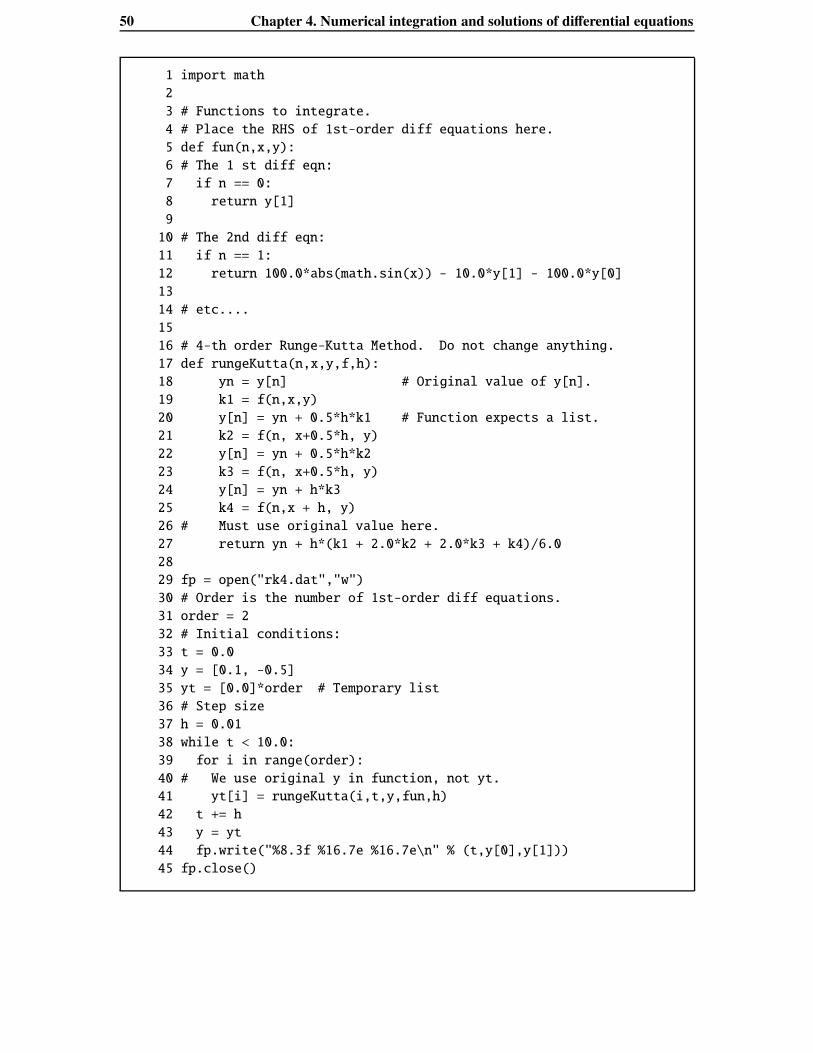
Below is an implementation of the RK4 algorithm for the problem of Ex. 2.1. We use a list, y,because we want to extend the code to differential equations of higher order. As in the Euler method,we use a function fun which evaluates and returns the RHS of each 1st order differential equation.In the rungeKutta function we start by saving the original value of y[n] to a temporary variable,yn, because we do not want to use the updated value of y[n] when evaluating each equation. Wereturn with the update value of y[n]. In the calling program, note that we use a temporary list, yt,to store the updated values of y (line 41), and that we call rungeKutta with the original values ofy. When all the equations have been evaluated, we update y (line 43).

The Runge-Kutta method is more accurate than the Euler method. For Ex. 2.1 and h = 0.1, themaximum error is 0.01; for h = 0.01 it is 0.001; for h = 0.001 it is 0.0001.


1 import math

2



5 def fun(n,x,y):


7 if n == 0:

8 return y[1]

9


11 if n == 1:

12 return 100.0*abs(math.sin(x)) - 10.0*y[1] - 100.0*y[0]

13

14 # etc....

15

16 # 4-th order Runge-Kutta Method. Do not change anything.

17 def rungeKutta(n,x,y,f,h):

18 yn = y[n] # Original value of y[n].

19 k1 = f(n,x,y)

20 y[n] = yn + 0.5*h*k1 # Function expects a list.

21 k2 = f(n, x+0.5*h, y)

22 y[n] = yn + 0.5*h*k2

23 k3 = f(n, x+0.5*h, y)

24 y[n] = yn + h*k3

25 k4 = f(n,x + h, y)

26 # Must use original value here.

27 return yn + h*(k1 + 2.0*k2 + 2.0*k3 + k4)/6.0

28

29 fp = open("rk4.dat","w")

30 # Order is the number of 1st-order diff equations.

31 order = 2

32 # Initial conditions:

33 t = 0.0

34 y = [0.1, -0.5]


36 # Step size

37 h = 0.01

38 while t < 10.0:


40 # We use original y in function, not yt.

41 yt[i] = rungeKutta(i,t,y,fun,h)

42 t += h

43 y = yt

44 fp.write("%8.3f %16.7e %16.7e\n" % (t,y[0],y[1]))

45 fp.close()

4.4. The Runge-Kutta method 51

0

0.2

0.4

0.6

0.8

1

0 0.2 0.4 0.6 0.8 1

a

t

"a""b""c""d""e"

Figure 4.3: Backwards evolution of the cosmic scale factor.

Exercises4.4.1 Although the actual size of our Universe is ”unmeasurable”, one usually describes distances

at different times (which will change due to expansion or contraction) in terms of a cosmicscale, R(t), with its present value denoted by R0 = R(t0). Additionally, one can normalize R(t)by its present value and define a cosmic scale factor, a(t) = R(t)/R0. The rate of change ofa(t) with time, a(t) = H0, is the present value of the Hubble parameter H0 = 73 km s−1 permegaparsec. The evolution of the scale factor with time is governed by the equation,

dadt =

√1 −Ω0 +

ΩMa +

ΩRa2 + a2Ωλ,

where Ω0 = ΩM +ΩR+Ωλ, is the total density parameter, ΩM is the relative density of matter(including dark matter), ΩR is the relative radiation energy density and Ωλ is the relative darkenergy density. In this equation the unit of time has been chosen so that the present age of theuniverse, t0 = 1. It is thought that currently the values are ΩM ≈ 0.3, ΩR ≈ 0, Ωλ ≈ 0.7.Use RK4 to determine the backwards evolution of the scale factor from its present value tothe start of the Big Bang at t = 0. Use a step size h = −0.01 to work backwards from theinitial condition t = 1, a = 1 and stop when t reaches zero. Plot a as a function of t for thefollowing choices:

(a) An empty Universe (ΩM = ΩR = Ωλ = Ω0 = 0).(b) The critical density case Ω0 = 1 with ΩM = 1,ΩR = Ωλ = 0.(c) Ω0 = 2 with ΩM = 2.0,ΩR = Ωλ = 0.(d) Ω0 = 1 with ΩM = 0.3, ΩR = 0, Ωλ = 0.7.(e) The steady state model with Ω0 = 1, Ωλ = 1, ΩM = ΩR = 0.

Plot all on one graph; compare your results with Fig. 4.3.


4.4.2 The gravitational potential, φ, is given by Poisson’s equation ∇2φ = 4πGρ where G is thegravitational constant and ρ(r) is the mass density. For the spherically-symmetric case, wehave

1r2

ddr

(r2 dφ

dr

)= 4πGρ

For stellar interiors the relationship ρ = λφn, where λ and n are constants, is a reasonableapproximation. Putting r = ax where

a2 =(n + 1)Kλ(1−n)/n

4πGresults in

1x2

ddx

(x2 dφ

dx

)= −φn.

At the centre of the star x = 0, φ = 1 and dφ/dx = 0.

(a) Show that when x ≈ 0, φ = 1 − 16 x2 and dφ/dx ≈ − 1

3 x.(b) Plot φ as a function of x for n = 3 and determine the value of x at the surface of the star

when φ = 0. [Answer x = 3.142]

4.5 Boundary value problemsSo far we have only considered solutions for differential equations where the boundary conditionsare specified at the same point. This is called an initial value problem (IVP). We may encountera differential equation where the boundary values are specified at different points. This is called aboundary value problem (BVP). As an example, suppose we want to know the deflection, y, of abeam supported at two ends, x = 0 and x = L. The differential equation is

d2ydx2 = ax(x − L)

where a is a constant. We know that the deflection will be zero at the two ends, so the boundaryconditions are y(0) = 0 and y(L) = 0. In this problem we are given two boundary conditions, asrequired to solve a second order differential equation, but they are specified at two different points.In order to solve this problem as an IVP, we need to know y′(0) or y′(L).

One way to solve a BVP like this is to guess the missing boundary condition, thereby turning itinto an IVP. In the example, we guess the value of y′(0), solve this IVP and obtain y(L). In general,y(L) will not have the required value. Using trial and error or some scientific approach, one makesanother guess at y′(0) and tries to get as close to the required boundary value as possible. This iscalled the shooting method because it is like aiming for a distant target with a gun.

We could try plotting the value of y(L) for different initial guesses of y′(0) and read off from thegraph what value of y′(0) is required to give the correct value of y(L). If the graph turns out to bea straight line, we only need two guesses. Suppose that the straight line can be written as y ′(0) =a0 + a1y(L). For our first guess y′1(0) = a0 + a1y1(L) and for the second guess y′2(0) = a0 + a1y2(L).Solving for the coefficients we obtain

y′(0) = y′1(0) +( y′2(0) − y′1(0)y2(L) − y1(L)

)(y(L) − y1(L)) .

So putting y(L) = 0 in this equation we can determine the required value of y′(0).Once we have obtained a better guess by using the value given by the straight line, we can use

this guess to see how close it takes us to the required value of y(L). In general, we will find that the

4.5. Boundary value problems 53

answer does take us closer to the required value, but not close enough for our purposes. In that casewe define a value, ε, which defines how close we want to get to the required value. If the value weobtain after using the straight line is yn(L), then we want to continue until |yn(L)− y(L)| < ε. If yn(L)does not satisfy this condition, we repeat the procedure until it is eventually satisfied.

Let us see how we can program this BVP using the 4-th order Runge-Kutta code we havedeveloped. If we let y0 = y and y1 = dy/dx, we have

dy0dx = y1,

dy1dx = ax(x − L).

In the example we will use a = 5 × 10−4 and L = 10. The code is shown below.

1 import math

2



5 def fun(n,x,y):


7 if n == 0:

8 return y[1]


10 if n == 1:

11 return 0.0005*x*(x - 10.0)

12

13 # 4-th order Runge-Kutta Method. Do not change anything.

14 def rungeKutta(n,x,y,f,h):

15 yn = y[n] # Original value of y[n].

16 k1 = f(n,x,y)

17 y[n] = yn + 0.5*h*k1 # Function expects a list.

18 k2 = f(n, x+0.5*h, y)

19 y[n] = yn + 0.5*h*k2

20 k3 = f(n, x+0.5*h, y)

21 y[n] = yn + h*k3

22 k4 = f(n,x + h, y)

23 # Must use original value here.

24 return yn + h*(k1 + 2.0*k2 + 2.0*k3 + k4)/6.0

25

26 # Integrates diff equation from x to x1

27 def ode(x,x1,h,y,fun,order):

28 while x < x1:


30 yt[i] = rungeKutta(i,x,y,fun,h)

31 x += h

32 return

33

34 # Calculates straight line coefs and returns value at y01

35 def fitline(y01,g1,g2,f1,f2):

36 a1 = (g2[1] - g1[1])/(f2[0] - f1[0])

37 a0 = g1[1] - a1*f1[0]

38 return a0 + a1*y01


39

40 order = 2

41 # Starting and ending value of x

42 x0 = 0.0

43 x1 = 10.0

44 #

45 # Initial value with guess for y1(x0)

46 y0_0 = 0.0

47 y1_0 = 0.1 # A guess

48 #

49 # Required value for y0(x1)

50 y0_1 = 0.0

51 #

52 # Tolerance, step size

53 eps = 1.0e-4

54 h = 0.01


56 #

57 # Initial guess

58 g1 = [y0_0, y1_0]

59 while 1:

60 # Integrate with first guess

61 y = [g1[0],g1[1]]

62 ode(x0,x1,h,y,fun,order)

63 # Test if required precision has been attained.

64 if abs(y0_1-yt[0]) < eps:

65 break

66 f1 = [yt[0], yt[1]]

67 # Take a second guess

68 g2 = [g1[0], g1[1]+0.1]

69 y = [g2[0],g2[1]]

70 # Integrate with second guess

71 ode(x0,x1,h,y,fun,order)

72 f2 = [yt[0],yt[1]]

73 # Fit a straight line and return new guess.

74 g1[1] = fitline(y0_1,g1,g2,f1,f2)

75 print "Initial conditions: ", g1

76 print "Boundary conditions: ", yt

We start at 40 by defining the order of the system (there are two 1st order equations, so order= 2). The starting and ending values of x are 0 and 10 respectively. The initial conditions arey0(0) = 0, but y1(0) is unknown and we have guessed y1(0) = 0.1. Any other guess will be equallyvalid. The required value of y0(L) = 0 (line 50). We define a tolerance of 1.0 × 10−4, meaning thatthe program will run until the initial guess leads to a value of y0(L) which differs from the requiredvalue by less than this amount. In line 54 we define the step size and create a temporary list, yt. Wekeep the initial conditions for the first guess in the list g1.

In line 59 we begin the loop which will continue until the tolerance level has been met. We startwith the first guess, g1, and integrate the differential equations all the way to x = L by calling thefunction ode. After the call, yt contains the boundary conditions at x = L. We store this in list f1

4.5. Boundary value problems 55

(Line 66). Then we take a second guess, g2, in which we simply increment y1(0) by 0.1 (line 68).We could have changed y1(0) by some other value, this does not matter because all we want to do isto take any two points so that we can fit a straight line. We then call ode again, this time using thesecond guess as initial values and store the boundary conditions in f2 (line 72).

So now we have two guesses, g1 and g2, at the initial conditions which result in the boundaryconditions f1 and f2 respectively. With this information we can fit a straight line to g as a functionof f by calling fitline. fitline calculates the straight line coefficients, a0 and a1 in y′(0) =a0 + a1y(L) or g[1] = a 0 + a 1f[0] and returns a better guess for y′(0), which is used as thenext initial guess.

What happens if the dependence of y′(0) on y(L) is not a straight line? In this case we willobtain a value for y′(0) which is closer to the true value than our initial guess. On the next iterationwe obtain an even better solution. The procedure is repeated until the specified tolerance is met.

The shooting method is conceptually easy to visualize, but sometimes it is not the best methodof solving a boundary value problem because the boundary conditions at the end point might bevery sensitive to the initial boundary conditions. This can sometimes be alleviated by choosing asuitable value of x = x f between the initial value, x = x0 and the final value x = x1 (x f is called afitting point). The shooting method is used to integrate from x0 to x f and also to integrate betweenx1 and x f . The idea is to choose initial values at x0 and x1 so that the values all match at the fittingpoint.

A very powerful method begins by transforming the system of differential equations to a systemof finite difference equations. For example, we can replace the differential equation

dydx = f (x, y)

with an algebraic equation relating function values at two points k and k − 1:

yk − yk−1 = (xk − xk−1) f(12

(xk + xk−1) , 12(yk + yk−1)

).

We are given values at some starting point k = k0 and at some end point, k = k1. We then havea system of coupled linear equations which can be solved at all values of k. This is called therelaxation method.

Exercises4.5.1 Find a solution for the boundary value problem

d2ydx2 = 0.0005x(x − 10)

with y(0) = 0 and y(10) = 0 and plot the beam displacement as a function of x. [Answer:y′(0) = 0.04166 at x = 0.]

4.5.2 Solve the boundary value problem

d2ydx2 = −

1(1 + y)2

with y(0) = y(1) = 0. [Answer: y′(0) = 0.43215.]

Chapter 5

Searching for hidden periods in data

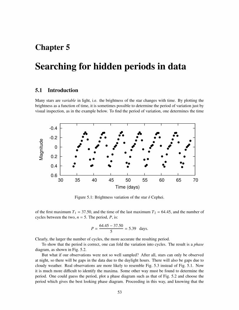
5.1 IntroductionMany stars are variable in light, i.e. the brightness of the star changes with time. By plotting thebrightness as a function of time, it is sometimes possible to determine the period of variation just byvisual inspection, as in the example below. To find the period of variation, one determines the time

-0.4

-0.2

0

0.2

0.4

0.6 30 35 40 45 50 55 60 65 70

Mag

nitu

de

Time (days)

Figure 5.1: Brightness variation of the star δ Cephei.

of the first maximum T1 = 37.50, and the time of the last maximum T2 = 64.45, and the number ofcycles between the two, n = 5. The period, P, is:

P = 64.45 − 37.505 = 5.39 days.

Clearly, the larger the number of cycles, the more accurate the resulting period.To show that the period is correct, one can fold the variation into cycles. The result is a phase

diagram, as shown in Fig. 5.2.But what if our observations were not so well sampled? After all, stars can only be observed

at night, so there will be gaps in the data due to the daylight hours. There will also be gaps due tocloudy weather. Real observations are more likely to resemble Fig. 5.3 instead of Fig. 5.1. Nowit is much more difficult to identify the maxima. Some other way must be found to determine theperiod. One could guess the period, plot a phase diagram such as that of Fig. 5.2 and choose theperiod which gives the best looking phase diagram. Proceeding in this way, and knowing that the

53

54 Chapter 5. Searching for hidden periods in data

-0.4

-0.2

0

0.2

0.4

0.6 0 0.2 0.4 0.6 0.8 1 1.2 1.4

Mag

nitu

de

Phase

Figure 5.2: Brightness variation folded with period P = 5.39 days.

-0.6

-0.4

-0.2

0

0.2

0.4

220 240 260 280 300 320 340

Mag

nitu

de

Time (days)

Figure 5.3: Actual observations of the star δ Cephei.

period is somewhere around 5.4 days, we can construct a large number of phase diagrams close tothis period (Fig. 5.4) and choose the one with smallest scatter.

Constructing phase diagrams in this way is a rather laborious enterprise. It would be betterif we could just calculate the scatter about the best-fitting curve without necessarily plotting thephase diagram. To do this we need to know the functional relationship between the brightness,V , and the time, t. We see that the curve is roughly sinusoidal (though there is definitely a fairdegree of asymmetry), so we may assume that the true brightness of the i-th observation is given byVT,i = a0 + A sin(ωti + φ). The angular frequency is ω = 2π

P . We cannot measure VT,i, instead wemeasure Vi, where VT,i = Vi + εi, and εi is the error in the observation. Thus we write

Vi + εi = a0 + A sin(ωti + φ)= a0 + A cos φ sinωti + A sin φ cosωti= a0 + a1 sinωti + a2 cosωti

where the amplitude A =√

a21 + a2

2. This kind of equation should now be familiar. Putting xi =

sinωti, and yi = cosωti, we see that this is just another example of multivariate least squares.

5.1. Introduction 55

-0.4

-0.2

0

0.2

0.4 0 0.2 0.4 0.6 0.8 1 1.2 1.4

Phase

-0.4

-0.2

0

0.2

0.4

Mag

nitu

de

-0.4

-0.2

0

0.2

0.4

Figure 5.4: Observations of Fig. 3 phased with P = 5.3 (top), 5.4 (middle) and 5.5 (bottom) days.

To find the solution which minimizes the sum of the squares of the errors,∑ε2i , we equate the

partial derivatives with respect to a0, a1 and a2 to zero and we end up with the following simultane-ous equations:

< V > = a0 + a1 < sinωt > +a2 < cosωt >< V sinωt > = a0 < sinωt > +a1 < sin2 ωt > +a2 < sinωt cosωt >< V cosωt > = a0 < cosωt > +a1 < sinωt cosωt > +a2 < cos2 ωt >

We could proceed in the usual way and solve these equations by matrix inversion. Since we willbe trying a large number of periods, and since we need a complete solution for each trial period,this will require a great deal of computation. Fortunately, some good approximations can be madewhich will allow an approximate solution without matrix inversion.

First, we assume that we have a large number of data points, in which case the mean of sinωtand cosωt will be very close to zero. This is simply due to the fact that the sine and cosine curvesspend an equal time being positive as being negative. Making this approximation we have from the


first equation a0 ≈< V >. In other words, the constant term is just the average value, < V >. Itis convenient to remove this constant term from the data, vi = Vi− < V >, so the remaining twoequations become

< v sinωt > = a1 < sin2 ωt > +a2 < sinωt cosωt >< v cosωt > = a1 < sinωt cosωt > +a2 < cos2 ωt >

Note that < sinωt cosωt >= 12 < sin 2ωt > should also be very close to zero. What is the average

of sin2 θ over a cycle? This is how we work it out:

< sin2 θ > =

∫ 2π0 sin2 θdθ∫ 2π

0 dθ=

12∫ 2π

0 (1 − cos 2θ)dθ2π

=12

2π2π=

12

We can see that < cos2 θ >= 12 as well. Making these approximations, we have

a1 ≈ 2 < v sinωt >, a2 ≈ 2 < v cosωt > .

The squared amplitude is

A2 = a21 + a2

2 = 4(< v sinωt >2 + < v cosωt >2

).

To determine the standard deviation, we note that

εi = a0 + a1 sinωti + a2 cosωti − Vi

= a1 sinωti + a2 cosωti − vi

Multiplying both sides by εi and forming averages we find

< ε2 > = a1 < ε sinωt > +a2 < ε cosωt > − < εv >The terms < ε sinωt >, < ε cosωt > are both approximately zero because the errors are random andsinωt and cosωt average out to zero. Therefore

< ε2 > ≈ − < εv >In terms of vi = Vi− < V >, our original model is

vi + εi = a1 sinωti + a2 cosωti

Multiplying this equation by vi, we have

< v2 > + < εv > = a1 < v sinωt > +a2 < v cosωt > .

Using < εv >≈ − < ε2 > and substituting for a1, a2, we finally have

< ε2 > ≈ < v2 > −2 < v sinωt >2 −2 < v cosωt >2 .

Given a particular value of ω = 2π/P, we can evaluate the quantities on the right-hand sideof this equation to obtain the standard deviation about the best-fitting sinusoid, σ =

√< ε2 >. By

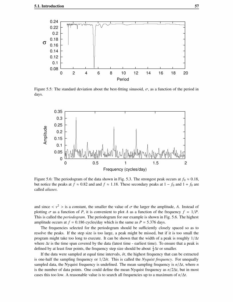
calculating σ for a large number of trial periods and by plotting σ as a function of P, the period forwhich σ is a minimum can be found. In Fig. 5.5 we show such a plot for the example discussedabove. The period which has minimum σ is found to be P = 5.376 days.

In practise, astronomers prefer not to use σ in this plot. We note that

< ε2 >= σ2 =< v2 > −12

A2

5.1. Introduction 57

0.08 0.1

0.12 0.14 0.16 0.18 0.2

0.22 0.24

0 2 4 6 8 10 12 14 16 18 20Period

σ

Figure 5.5: The standard deviation about the best-fitting sinusoid, σ, as a function of the period indays.

0 0.05 0.1

0.15 0.2

0.25 0.3

0.35

0 0.5 1 1.5 2

Ampl

itude

Frequency (cycles/day)

Figure 5.6: The periodogram of the data shown in Fig. 5.3. The strongest peak occurs at f0 ≈ 0.18,but notice the peaks at f ≈ 0.82 and and f ≈ 1.18. These secondary peaks at 1 − f0 and 1 + f0 arecalled aliases.

and since < v2 > is a constant, the smaller the value of σ the larger the amplitude, A. Instead ofplotting σ as a function of P, it is convenient to plot A as a function of the frequency f = 1/P.This is called the periodogram. The periodogram for our example is shown in Fig. 5.6. The highestamplitude occurs at f = 0.186 cycles/day which is the same as P = 5.376 days.

The frequencies selected for the periodogram should be sufficiently closely spaced so as toresolve the peaks. If the step size is too large, a peak might be missed, but if it is too small theprogram might take too long to execute. It can be shown that the width of a peak is roughly 1/∆twhere ∆t is the time span covered by the data (latest time - earliest time). To ensure that a peak isdefined by at least four points, the frequency step size should be about 1

4∆t or smaller.If the data were sampled at equal time intervals, δt, the highest frequency that can be extracted

is one-half the sampling frequency or 1/2δt. This is called the Nyquist frequency. For unequallysampled data, the Nyquist frequency is undefined. The mean sampling frequency is n/∆t, where nis the number of data points. One could define the mean Nyquist frequency as n/2∆t, but in mostcases this too low. A reasonable value is to search all frequencies up to a maximum of n/∆t.


0

0.05

0.1

0.15

0.2

0.25

0.3

0 1 2 3 4 5 6 7 8 9 10

Ampl

itude

Frequency (cycles/day)

Figure 5.7: Periodogram of a star with P = 0.187 days showing the aliasing caused by daytime gapsin the data.

Exercises5.1.1 Write a program that reads the the time (in days) and the magnitude from file cepheid.dat.

The program should ask for the period and then write the phase and magnitude to another file.Ensure the phase, φ, is in the range < φ < 1.5 and plot the phase diagram. The true period isbetween 5.2 < P < 5.6 days. Determine the period by visual inspection of the phase diagram.

5.1.2 Write a program which asks for the starting frequency, stopping frequency and frequency stepsize. The program then reads a file containing the time, t, and magnitude, V , for a variablestar. Store these values in separate python lists. For each frequency, f , the program calculatesthe amplitude A = 2

√< v sinωt >2 + < v cosωt >2, and writes f , A to an output file. Apply

the program to the data in file cepheid.dat and

(a) plot the periodogram and visually locate the frequency of maximum amplitude;(b) use the polynomial-fitting program to fit a quadratic to A as a function of f . Find the

maximum of the quadratic and hence the best value of f .

5.2 AliasesIn Fig. 5.6, which is the periodogram of the data in Fig. 5.3, we see that in addition to the large peakat f1 = 0.186 cycles/day, there are smaller peaks at f2 = 0.814 and f3 = 1.186 cycles/day. Note thatf2 = 1 − f1 and f3 = 1 + f1. These two peaks arise because there are gaps in the data set. Becausethe data in Fig. 5.3 could only be obtained at night, there is a gap of about one day between eachmeasurement (sometimes more than one day if the night was cloudy). Because of these gaps, onecould squeeze in an extra cycle or leave out a cycle and still get a reasonable fit to the sinusoid. Thiseffect is responsible for the two weaker peaks which are called aliases.

Aliases are separated from the true peak by the frequency at which the data were sampled. Inastronomical observations done from a single site, the sampling frequency is 1 cycle/day so that onealways obtains aliases separated by 1 cycle/day from the true frequency. Aliasing occurs in any dataset which is not completely sampled. The more frequent the gaps, the larger the amplitude of thealias peaks. In some cases it is not possible to determine a unique frequency because the aliases areso strong.

Fig. 5.7 shows a periodogram which illustrates the concept of aliases rather clearly. This peri-odogram is of a star with a period P = 0.187 days or f = 5.345 cycles/day. Notice that the highest

5.3. Harmonics 59

peak does, indeed have a frequency f = 5.345, but notice the 1 cycle/day aliases at 4.345 and 6.345cycles/day. In this data set, there are frequent gaps lasting for 2 days so that the 2 cycle/day aliasesat 3.345 and 7.345 cycles/day are also quite strong. The other, smaller peaks are also due to aliasing.

5.3 Harmonics

In the model we have been using, we assume that the data is well represented by a pure sinusoid

Vi + εi = a0 + A sin(ωti + φ).

This may be a good approximation in many cases, but not in others as shown in Fig. 5.8. This isthe light curve of the RR Lyrae star SS Leo which shows a very steep rise in brightness followedby a gradual decline. The actual data from which the phase diagram of Fig. 5.8 was constructed isshown in Fig. 5.9. Notice the very uneven data sampling and the large gaps.

The periodogram of SS Leo is shown in Fig. 5.10. First of all, notice that there are several peaksof almost equal height at f = 0.60, 1.60, 2.20, 2.60, 3.20 and 4.20 cycles/day. These correspond toperiods of 1.67, 0.62, 0.45, 0.38, 0.31, and 0.24 days. It is clear, however, that at least some of thefrequencies 0.60, 1.60 and 2.60 cycles/day are aliases owing to the daily gaps in the data. The trueperiod is 0.6263441 days which is f = 1.60 cycles/day. Therefore the peaks at 0.60 and 2.60 arealiases. In this case it is almost impossible to select the correct period owing to severe aliasing.

The other sequence of peaks at 2.23, 3.23 and 4.23 cycles/day also seem to be mostly aliases,but this time it is due to the highly non-sinusoidal nature of the variations. The light curve is poorlyrepresented by a sine wave, but it is better described by a sine wave with frequency f = 0.61cycles/day together with the first harmonic at twice the frequency, f = 1.20 cycles/day. Therefore3.20 and 4.20 are the aliases of the first harmonic. Thus the periodogram is well described by justtwo frequencies, 0.60 and 1.20 cycles/day, and their 1 cycle/day aliases. The second harmonic atf = 1.80 cycles/day is also present, but is much weaker.

This example, although extreme, illustrates the limitations of the method. To describe the lightcurve of SS Leo accurately requires several Fourier components and not just the fundamental fre-quency. As a result the power that would otherwise be concentrated in the fundamental frequencyis spread over several components, lowering the amplitudes. In this example we have, in addition,observations which are sparse and include large gaps. This further complicates the periodogramwhich now includes not only the two Fourier components of highest amplitude (the fundamentaland first harmonic), but also their 1 cycle/day and 2 cycle/day aliases. Under these circumstances,it is best to use a different period finding technique.

Exercises

5.3.1 Calculate and plot the periodogram of the data in file dsct.dat between 0 and 10 cycles/day.

(a) Find the most likely frequency [Answer: 4.789 cycles/day].

(b) Use the Fourier analysis program in Chapter 3, Section 4 to compute the Fourier co-efficients which best fit these data at this frequency. [Answer: a0 = 8.456144, A1 =0.099895, φ = 2.343396 radians]

(c) Use the program in Ex. 5.1.1 to construct a phase diagram and plot the phase diagramwith the fitted Fourier curve.


10.2

10.4

10.6

10.8

11

11.2

11.4

11.6 0 0.2 0.4 0.6 0.8 1 1.2 1.4

Mag

nitu

de

Phase

Figure 5.8: Light curve of SS Leo (period 0.6263441 days) showing large departure from a puresinusoid.

10.2 10.4 10.6 10.8

11 11.2 11.4 11.6

0 5 10 15 20 25 30 35

Mag

nitu

de

Days

Figure 5.9: Data of Fig. 5.8 plotted versus time in days.

0 0.05

0.1 0.15

0.2 0.25

0.3 0.35

0.4

0 0.5 1 1.5 2 2.5 3 3.5 4 4.5 5

Ampl

itude

Frequency

Figure 5.10: Periodogram of data in Fig. 5.9.

5.4. Multiperiodic variations 61

5.4 Multiperiodic variations

Harmonics (multiples of the fundamental frequency) as discussed above are not really independentperiods since they are just a consequence of departure from a pure sinusoid. Many stars pulsate inmore than one period. For example some δ Scuti stars have 3, 4, 5 or even more periods. We extractthe frequencies in such data in the same way as we do for the case of just one period - by using theperiodogram.

Fig. 5.11 shows the periodogram of a δ Scuti star with three periods. Note that one can immedi-ately pick out the frequency with the highest amplitude at f1 = 7.156 cycles/day and another one ata frequency close to 5 cycles/day. The periodogram is very clean and we note that the 1 cycle/dayaliases are very small. This is due to the fact that the star was observed from three continents roundthe clock - from Australia, South Africa and Chile.

In order to be able to detect further frequencies, we need to remove the frequency of highestamplitude from the original data. This process is called prewhitening. We fit a Fourier curve to thedata using the known frequencies and subtract the fitted Fourier curve from the data. In other words,we find the least-squares solution to

Vi + εi = a0 + a1 sin 2π f1ti + a2 cos 2π f1ti+ a3 sin 2π f2ti + a4 cos 2π f2ti+ a5 sin 2π f3ti + a6 cos 2π f3ti + . . .

where f1, f2, f3, . . . are the frequencies so far extracted. Using the solution, we calculate the value ofV at time, t, subtract the calculated value, Vci, from the observed value, Vi and write ti and Vi−Vci toa new file. A new periodogram is calculated and the next frequency is determined until the peak isnot high enough to distinguish it from noise. The program listed below implements this procedure.

Fig. 5-11 to 5-14 is an example of this procedure. The periodogram of the original data inFig. 5.11 gives f1 = 7.156 cycles/day. Fitting and removing the sinusoid with this frequency givesthe periodogram in Fig. 5-12 from which we find the next frequency, f2 = 4.921 cycles/day. Fittingthe original data by f1 and f2 gives Fig. 5-13 from which we obtain f3 = 5.345 cycles/day. Remov-ing f1, f2, f3 from the original data gives Fig. 5-14. The highest peak is only about twice the heightof the noise and we cannot therefore be certain that it is real. There is no definite criterion to judgewhether a peak is real or not, but a general rule of thumb is not to accept peaks unless they are atleast 4 times higher than the background noise. We conclude that there are three certain frequenciesin this star: f1 = 7.156, f2 = 4.921 and f3 = 5.345 cycles/day.

We chose a data set where the aliases were of very low amplitude. More often than not, thealiases are at least half the height of the main peak and it may become impossible to decide onwhether a frequency is real or an aliases, especially if it is close to an aliases of another frequency.

Exercises

5.4.1 Using the program of Ex. 1.2 (calculating the periodogram) and the program listed on page 10(prewhitening with given frequencies), determine the frequencies present in file multiperiod.dat.These are the data used to generate Fig. 5.11 to 5.14 and you should obtain the same frequen-cies.


0

0.005

0.01

0.015

0.02

0.025

0 1 2 3 4 5 6 7 8 9 10

Ampl

itude

Frequency

Figure 5.11: Periodogram of a star with three frequencies.

0 0.002 0.004 0.006 0.008

0.01 0.012 0.014 0.016 0.018

0 1 2 3 4 5 6 7 8 9 10

Ampl

itude

Frequency

Figure 5.12: The periodogram of data prewhitened by f1 = 7.156 cycles/day.

0

0.001

0.002

0.003

0.004

0.005

0.006

0 1 2 3 4 5 6 7 8 9 10

Ampl

itude

Frequency

Figure 5.13: The periodogram of data prewhitened by f1 and f2 = 4.921 cycles/day.

0

0.0001

0.0002

0.0003

0.0004

0.0005

0.0006

0 1 2 3 4 5 6 7 8 9 10

Ampl

itude

Frequency

Figure 5.14: The periodogram of data prewhitened by f1, f2 and f3 = 5.345 cycles/day.

5.4. Multiperiodic variations 63

from numpy import *

import math

twopi = 2.0*math.pi

# Function to calculate the magnitude from the Fourier components.

def fourier(nf,f,A,t):

yc = 0.0


wt = twopi*f[k-1]*t

yc += A[2*k-1]*math.sin(wt)+ A[2*k]*math.cos(wt)

return yc + A[0]

f = []

nf = int(raw_input("Number of frequencies? "))

for i in range(nf):

str = raw_input("Frequency %d? " % (i+1))

f.append(float(str))

fp = open("data.in","r")

m1 = 2*nf + 1

x = zeros((m1,m1))

y = zeros((m1,1))

xi = [0.0]*m1

n = 0

day = []

mag = []

for line in fp:

t = float(line.split()[0])

yi = float(line.split()[1])

day.append(t)

mag.append(yi)

xi[0] = 1.0


wt = twopi*f[k-1]*t

xi[2*k-1] = math.sin(wt)

xi[2*k] = math.cos(wt)

for j in range(m1):

for k in range(m1):

x[j,k] += xi[j]*xi[k]

y[j,0] += yi*xi[j]

n += 1

fp.close()

X = mat( x.copy() )

Y = mat( y.copy() )

A = X.I*Y

# Remove Fourier fit from data and write prewhitened data.

fp = open("data.pre","w")

for i in range(n):

dmag = mag[i]- fourier(nf,f,A,day[i])

fp.write("%10.4f %10.4f\n" % (day[i],dmag))

fp.close()

numerical methods with python - florida...

Documents