numerical methods for ordinary …the thesis develops a number of algorithms for the numerical sol...
TRANSCRIPT
NUMERICAL METHODS FOR ORDINARY DIFFERENTIAL EQUATIONS
WITH APPLICATIONS TO PARTIAL DIFFERENTIAL EQUATIONS
A thesis submitted for the degree of
Doctor of Philosophy
by
Abdul Qayyum Masud Khaliq
Department of Mathematics and Statistics, Brunel University
Uxbridge, Middlesex, England. UB8 3PH
February 1983
.,~& ,
(i)
ABSTRACT
The thesis develops a number of algorithms for the numerical sol
ution of ordinary differential equations with applications to partial
differential equations. A general introduction is given; the existence
of a unique solution for first order initial value problems and well
known methods for analysing stability are described.
A family of one-step methods is developed for first order ordinary
differential equations. The methods are extrapolated and analysed for
use in PECE mode and their theoretical properties, computer implementation
and numerical behaviour, are discussed.
La-stable methods are developed for second order parabolic partial
differential equations 1n one space dimension; second and third order
accuracy 1S achieved by a splitting technique 1n two space dimensions.
A number of two-time level difference schemes are developed for first
order hyperbolic partial differential equations and the schemes are ana
lysed for Aa-stability and La-stability. The schemes are seen to have
the advantage that the oscillations which are present with Crank-Nicolson
type schemes, do not arise.
A family of two-step methods 1S developed for second order periodic
initial value problems. The methods are analysed, their error constants
and periodicity intervals are calculated. A family of numerical methods
is developed for the solution of fourth order parabolic partial differ
ential equations with constant coefficients and variable coefficients and
their stability analyses are discussed.
The algorithms developed are tested on a variety of problems from
the literature.
(ii)
ACKNOWLEDGE~ffiNTS
I would like to express my gratitude to my superv~sor Dr. E.H. Twizell
for his invaluable suggestions, continuous encouragement and
constructive criticism during both the period of research and the
writing of the thesis. He has always given patiently of his time and
his endeavours have extended well beyond the bounds of mere supervision.
I have learned a great deal from him and, for all that he has done, I
am deeply grateful.
I am also indebted to Professor J.Ll. Morris, Mr. G.D. Smith and
Professor J.R. Whiteman for many helpful discussions.
Finally, I wish to thank the British Government for its partial
support in tuition fees under the Overseas Research Students Fees
Support Scheme during the period 1981 - 1983.
(iii)
1I0ccupying a un1que place along the border between applied-
.mathematics and the concrete world of industry, the numerical
solution of differential equations, probably more than any other
branch of numerical analysis, is in a constant state of unrest
and evolution. Being so widely and variously applied in the real
world, its techniques are relentlessly put to the ruthless test of
practical success and usefulness. Nor does it evolve solely through
the cross influences of the practical necessities of engineering;
unusual impetus is also given to this field by the outstanding
advances in computer technology, which 1S gathering now to min-
iaturize hardware to lower the cost of the equipment, the arith-
metic, the logic, the storage, and the output that is made more
comprehensively grasped by directly presenting it to that most re-
markable of the human senses-vision, through computer graphics,
shifting thereby the engineer's or programmer's priorities 1n se-
lecting the most appropriate solution algorithm".
Isaac Fried, 1979.

CHAPTER 1
CHAPTER 2
2. 1
2.2
2.3
2.4
2.5
2.6
2.7
2.8
2.9
CHAPTER 3
3. 1
3.2
3.3
3.4
3.5
3.6
3.7
3.8
CONTENTS
INTRODUCTION
ONE-STEP METHODS FOR FIRST ORDERORDINARY DIFFERENTIAL EQUATIONS
Introduction
Derivation of the formulas
Analyses of the methods
Mathematical modelling of a Chemistry problem
Extrapolation of the methods
Use in PECE mode
Stability regions
Numerical examples
Conclusions
SECOND ORDER PARABOLIC EQUATIONS
Introduction
One-space dimension
A second order method and its extrapolation
Two third order methods and their extrapolations
A fourth order method
Numerical results
Two space dimensions
Second order method and its extrapolation
12
12
14
15
21
26
39
45
53
58
60
60
62
64
67
70
72
74
77
CHAPTER 4
4. 1
4.2
4.3
4.4
4.5
4.6
4.7
FIRST ORDER HYPERBOLIC EQUATIONS
Introduction
Central difference approximation 1n space
Low order (one-sided) approximation 1n space
A higher order space replacement
Higher order time replacements
Numerical experiments
Conclusions
84
84
86
88
93
96
101
108
CHAPTER 5 SECOND ORDER PERIODIC INITIAL VALUE PROBLEMS 113
5. 1 Introduction 113
5.2 Development of the methods 115
5.3 Analyses 117
5.4 Numerical examples 120
5.5 Use in PECE mode 125
5.6 Conclusions 130
CHAPTER 6 FOURTH ORDER PARABOLIC EQUATIONS 131
6. 1 Introduction 131
6.2 A recurrence relation 132
6.3 Solution at first time step 134
6.4 Development and analyses of the methods 135
6.5 Numerical results and discussion 139
6.6 Two-space variable case 144
APPENDICES
REFERENCES
149
155
( j )
CHAPTER 1
INTRODUCTION
Consider the first-order initial value problem
(1. 1) y' = f(x,y), y(a) = T) •
The following theorem outlined in Lambert (1973), with proof
contained in Henrici (1962), states conditions on f(x,y) which
guarantee the existence of a un1que solution of the initial value
problem (I. 1) •
Theorem 1.1
Let f(x,y) be defined and continuous for all points (x,y)
1n the region D defined by - 00 <y<oo, a and b
finite, and let there exist a constant L such that, for every
x,y,y* such that (x,y) and (x,y*) are both in D,
(1 .2) If(x,y) - f(x,y*)1 ~ L I y-y* I .
Then, if T) is any glven number, there exisma un1que solution y(x)
of the initial value problem (1.1), where y(x) is continuous and
differentiable for all (x,y) 1n D.
The requirement (1.2) 1S known as a Lipschitz condition, and the
constant L as a Lipschitz constant. This condition may be thought
of as being intermediate between differentiability and continuity, in
the sense that
f(x,y) continuously differentiable with respect to y for all
(x,y) r n D
~ f(x,y) satisfies a Lipschitz condition with respect to y for all
(x , y) t.n D
~ f(x,y) continuous with respect to y for all (x,y) 1n D.
In particular, if f(x,y) possesses a continuous derivative with respect
to y for all (x,y) 1n D, then, by the mean value theorem,
f(x,y) - f(x,y*) = af(x,y)By (y-y*),
(2)
where y ~s a point ~n the interior of the interval whose end-
points are y and y*, and (x,y) and (x,y*) are both ~n D.
Clearly, (1.2) is then satisfied if L ~s chosen to be
(l .3) L = sup I af ~yX,y) I .(x , y)e: D a
In many areas such as control theory, chemical kinetics and
biology, the dynamic behaviour is modelled, not with a single
differential equation, but with a system of m simultaneous first-
order equations in m dependant variables Yl' Y2' ... Ym. If each
of these variables satisfies a g~ven condition at the same value a of x
then the initial value problem for a first-order system may be written as
(l .4) y' =1 f 1(x'YI'Y2'···'Ym) ,
y' = f 2 (x,y I 'Y2'··· 'Ym) Y2 (a). = n22,
, I II t II II I
y' = fm(x'YI 'Y2'··· ,Ym)Y (a) = nm m m
Introducing the vector notation
T(n I ' n2' ..• , nm) ,
T denoting
as
(l . S)
transpose, the initial-value problem (1.4) may be written
Theorem 1.1 readily generalises to give necessary conditions for the
existence of a unique solution to (I.S); all that is required is that
the region D now be defined by a ~ x ~ b ,
and (1.2) be replaced by the condition
- 00 < y. < 00,
~
i. = 1,2, ... ,m,
(I .6)
where (x,~) and (x,~*) are ~n D, and I I. I I denotes a vector norm.
For the properties of vector and matrix norms see,for example, Mitchell
and Griffiths (1980). In the case when each of the f i(x'YI'Y2'···'Ym) ,
~ = 1,2, ... ,m, possesses a continuous derivative with respect to each of
(3)
the y ., J = 1,2, ... , m, thenJ
( 1 .7)
may be chosen analogously to (1.3), where a~/al 1S the Jacobian of
f with respect to l - that is, the m x m matrix whose i,jth
element 1S af. (x'Yl'Y2"'.'y lay., and I1.1 I denotes a matrix1 m J
norm subordinate to the vector norm employed in (1.6).
The first order system (1.5), namely ~' = ~(x,y), where ~
and fare m-dimensional vectors, is said to be linear if
f(x,y) = A(x)l + ~ (x) ,
where A(x) 1S an m x m matrix and ~(x) an m-dimensional vector;
if, in addition, A(x) = A, a constant matrix, the system is said to be
linear with constant coefficients. To find the general solution of the
system
(I .8) l' = Ay" + ~(x) ,
let y(x) be the general solution of the corresponding homogeneous system·
(I .9)
If ~(x) 1S any particular solution of (1.8), then
1S the general solution of (1.8). A set of solutions lk(x), k = 1,2, ... ,m,
of (1.9) is said to be linearly independent if
mL aklk(x):: Q ,
k=l
implies ~ = 0, k = 1,2, ... ,m. The general solution of (1.9) may be
written as a linear combination of the members of a set of m linearly
independent solutions
that
Yk(x), k = 1,2, ... ,m. It can easily be seen
(1.10)
where ~k 1S an m-dimensional vector, 1S a solution of (1.9) if
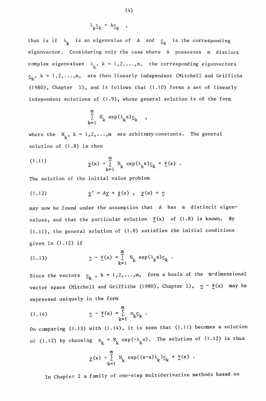
(4)
that is if Ak 1S an eigenvalue of A and £k 1S the corresponding
eigenvector. Considering only the case where A possesses m distinct
complex eigenvalues Ak
, k = 1,2 .... ,m. the corresponding eigenvectors
£k' k = I,2, ... ,m, are then linearly independent (Mitchell and Griffiths
(1980), Chapter 1), and it follows that (1.10) forms a set of linearly
independent solutions of (1.9), whose general solution is of the form
mL Nk exp(Akx)£k
k=I,
where the Nk
, k = 1,2, ... ,m are arbitrary constants. The general
solution of (1 .8) is then
(1.11)m
y(x) = L Nk exp(AkX)£k + !(x) .k=1
The solution of the initial value problem
(1.12)
may now be found under the assumption that A has m distincit e1gen-
values, and that the particular solution !(x) of (1.8) is known. By
(1.11), the general solution of (1.8) satisfies the initial conditions
given in (1.12) if
(1 . 13)m
~ - !(a) = L Nk exp(Aka)£k .k=1
Since the vectors £k' k = 1,2, ... ,m, form a basis of the m-dimensional
(1.14)
vector space (Mitchell and Griffiths (1980), Chapter 1), n - !(a) may be
expressed uniquely in the form
m
n - !(a) = L ~£k'k=l
On compar1ng (1.13) with (1.14), it is seen that (1.11) becomes a solution
of (1.12) by choosing ~ = Nk
exp(-Aka). The solution of (1.12) is thus
my(x) = L N
kexp{(x-a)Ak}£k + ~(x)
k=1
In Chapter 2 a family of one-step multiderivative methods based on
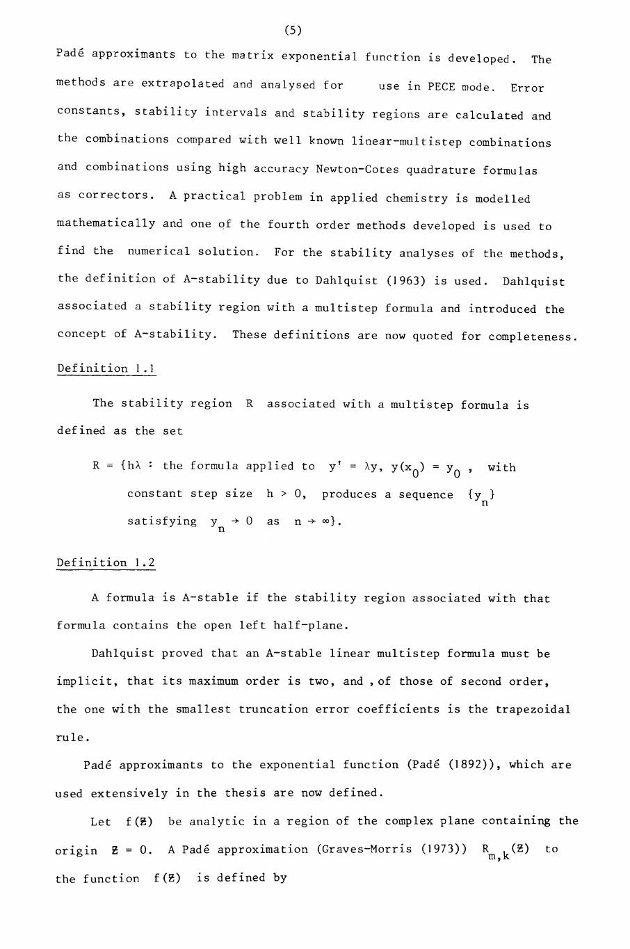
(5)
Pade approximants to the matrix exponential function ~s developed. The
methods are extrapolated and analysed for use ~n PECE mode. Error
constants, stability intervals and stability reg~ons are calculated and
the combinations compared with well known linear-multistep combinations
and combinations using high accuracy Newton-Cotes quadrature formulas
as correctors. A practical problem in applied chemistry is modelled
mathematically and one of the fourth order methods developed is used to
find the numerical solution. For the stability analyses of the methods,
the definition of A-stability due to Dahlquist (1963) is used. Dahlquist
associated a stability region with a multistep formula and introduced the
concept of A-stability. These definitions are now quoted for completeness.
Definition 1.1
The stability reg~on R associated with a multistep formula is
defined as the set
R = {hA : the formula applied to y' = AY, y(xO)
= YO' with
constant step s~ze h > 0, produces a sequence {y }n
satisfying
Definition 1.2
y ~ 0n
as n ~ oo}.
A formula is A-stable if the stability reg~on associated with that
formula contains the open left half-plane.
Dahlquist proved that an A-stable linear multistep formula must be
implicit, that its maximum order is two, and, of those of second order,
the one with the smallest truncation error coefficients is the trapezoidal
rule.
Pade approximants to the exponential function (Pade (1892)), which are
used extensively in the thesis are now defined.
Let f(~) be analytic in a region of the complex plane containing the
or1g~n ~ = O. A Pade approximation (Graves-Morris (1973))
the function f(~) ~s defined by
R k(~)m,to
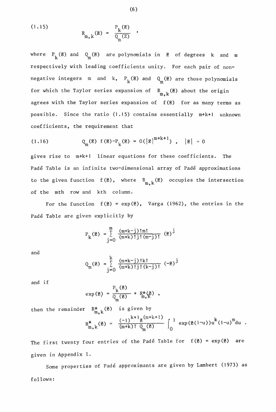
(6 )
(l.15)R k(B) =m,
,
Q (B)m
are polynomials 1n B of degrees k and m
respectively with leading coefficients unity. For each pair of non-
negative integers m and k, Q (B) are those polynomialsm
for which the Taylor series expansion of
agrees with the Taylor series expansion of
R k(B) about the originm,
feB) for as many terms as
possible. Since the ratio (1.15) contains essentially m+k+1 unknown
coefficients, the requirement that
(1.16)
glves r1se to m+k+l linear equations for these coefficients. The
Pade Table 1S an infinite two-dimensional array of Pade approximations
to the glven function feB), where R k(B)m,
occupies the intersection
of the mth row and kth column.
For the function feB) = exp(B), Varga (1962), the entries in the
Pade Table are given explicitly by
=! (m+k-j)!m! (B)J(m+k)!j! (m-j)!
j=O
and
= ~ (m+k-j)!k! (-B)JL (m+k)!j! (k-j)!
j=O
and if
+ R*(B) ,m,'K
then the remainder R* k(B)m,
R* (B) =m,k
is given by
(-I )k+IB(m+k+l)
(m+k)! ~ (B) [1 k mexp(B(I-u))u (l-u) du .
o
The first twenty four entries of the Pade Table for f(~) = exp(B) are
given in Appendix I.
Some properties of Pade approximants are glven by Lambert (1973) as
follows:
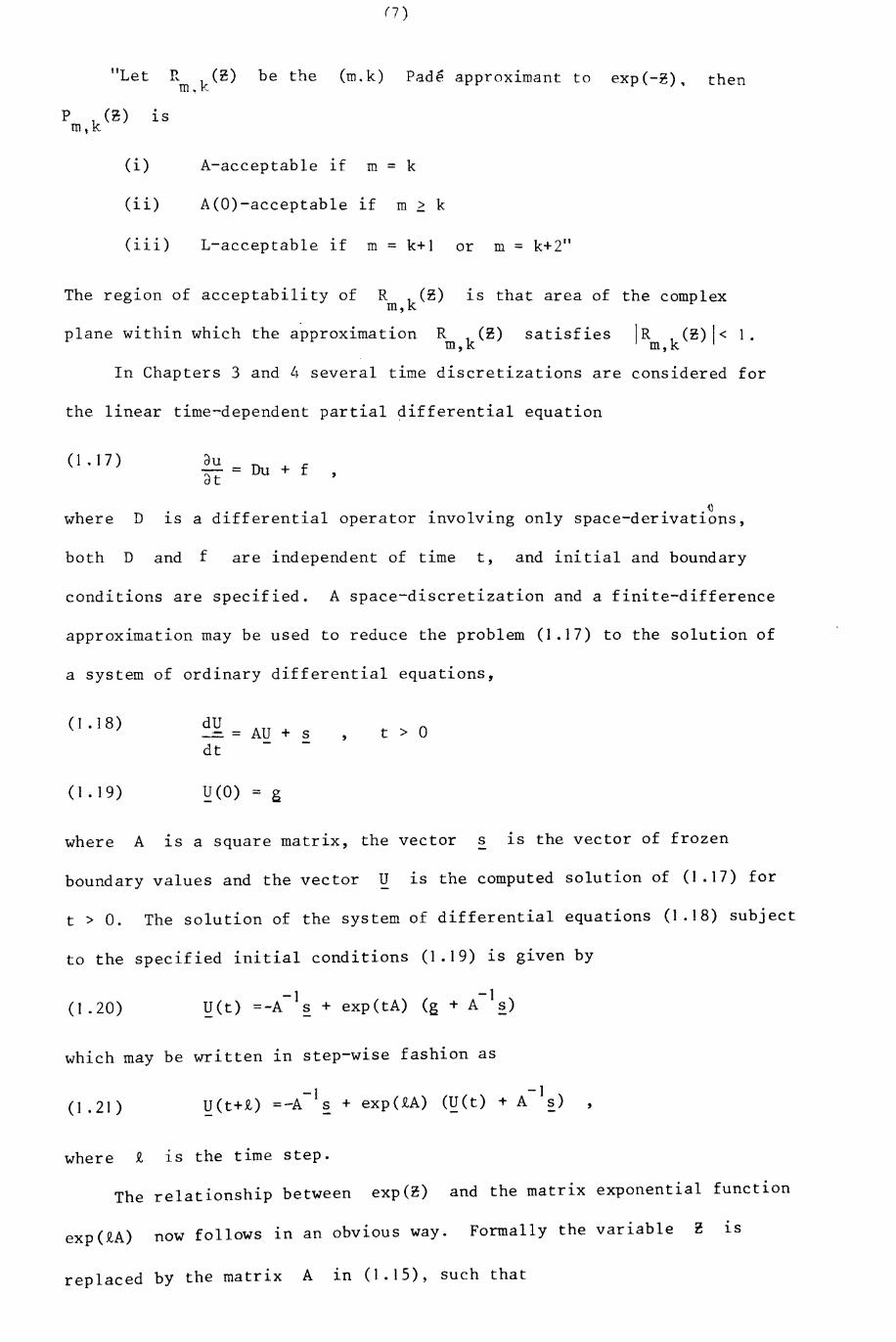
0)
"Let n\.m. k (2) be the ( k) P d" .~\ _ ~ - m. a e approx1mant to exp(-~). then
P k(l)m,.1S
(i) A-acceptable if m = k
(ii) A(O)-acceptable if m ~ k
(iii) L-acceptable if m = k+l or m = k+2"
The reg10n of acceptability of R k(~) 1S that area of the complexm,
plane within which the approximation Rm,k(l) satisfies IRm,k(l)1< 1.
In Chapters 3 and 4 several time discretizations are considered for
the linear time-dependent partial differential equation
(1.17) dU-=Du+fdt
where D 1S a differential operator involving only space-derivati0ns,
both D and f are independent of time t, and ini tial and boundary
conditions are specified. A space-discretization and a finite-difference
approximation may be used to reduce the problem (1.17) to the solution of
a system of ordinary differential equations,
(1.18) dU
dt= AU + s , t > 0
(1.19) !:!(O) = g
where A 1S a square matrix, the vector s 1S the vector of frozen
boundary values and the vector U 1S the computed solution of (1.17) for
t > O. The solution of the system of differential equations (1.18) subject
to the specified initial conditions (1.19) is given by
(I.20)
which may be written in step-wise fashion as
(1.21)
where £ 1S the time step.
The relationship between expel) and the matrix exponential function
exp(£A) now follows in an obvious way. Formally the variable l 1S
replaced by the matrix A in (1.15), such that
is the (m,k) Pade approximation of exp(£A). The relationship between
certain well-known numerical methods and the matrix Pade approximations
may be shown, for example, by approximating the matrix exponential
exp(£A) of equation (1.21) by the entry
Table to gi.ve
(1.22) 1 -1 1 -1-1= (1- 2tA) (I+ztA) (!!(t)-A §.)+A ~
which, 1n implicit form, is
( 1 .23)
Equation (1.23) defines the Crank-Nicolson method applied to equation
(1.18) if A is a tridiagonal matrix with the entry -2 on the diagonal
and on the super-and sub-diagonals. In a similar manner it can be
shown that RO,I (tA) and approximations generate respectively
the well known explicit and fully implicit methods for second order para-
bo1ic partial differential equations, see for example, Lawson and Morris
(1978) and Smith and Twize11 (1982). However, it is shown in Lawson and
Morris (1978), that the (1,1) Pade approximant, (the Crank-Nicolson
method) is an A-stable method and is less than satisfactory when a time
discretization is used with time step which is too large relative to the
spatial discretization.
In Chapter 3 a family of methods 1S developed for second order para-
bo1ic partial differential equations, which do not suffer from this
feature. Second and third order accuracy is achieved in two space di-
mensions by a splitting technique. The methods are tested on two problems
from the literature. The behaviours of the methods are also shown
graphically. Stability of the methods is analysed by two well known
methods; the von Neumann method and the Matrix method, which are now
mentioned briefly. For full details, see for example, Smith (1978) and
Mitchell and Griffiths (1980).
The von Neumann Method, developed by J. von Neumann and first discussed
(9)
1n detail by O'Brien et al (1951), provides a simple necessary con-
dition for numerical stability, and essentially depends on the uniform
boundedness of the Fourier coefficients of the solution of the differ-
ence equation. It 1S assumed that there exist harmonic decompositions
of the grid functions Uk at the initial time level and writes
= LA. exp(iS.xk)j J J
where i = ~ , the frequencies S.J
are, 1n general use, arbitrary,
and a uniform grid is used. It is only necessary to consider the single
term exp(iSx) where S 1S any real number and to use the superposition
principle for linear problems. To investigate the growth of the grid
functions as t increases for any value of S, it is necessary to find
a solution of the difference equation which reduce to exp(iSx) when
t = O. Such a solution is
exp(at) exp(iSx)
where a = a(S) 1S, 1n general, complex. The original grid function
exp(iSx) will not grow with time if
(1.23) lexp(a£) I ~
where £ 1S the increment in t. This is the von Neumann necessary
criterion for stability; this technique of analysing stability 1S
called the von Neumann Method. The following points concern1ng the von
Neumann method are worth mentioning:
(i) The method only applies rigorously if the coefficients of
the linear difference equation are constant; though it is
conventional to apply it locally when the coefficients are
not constant.
(ii) For two level difference schemes with one dependent variable
and any number of independent variables the von Neumann
condition is sufficient as well as necessary for stability,
otherwise the condition 1S only necessary.
(iii)
,j v)
Boundary conditions are neglected 1n the von Neumann
analysis and hence, 10 theory, it only applies to pure
initial value problems with periodic initial data.
It is noted that stability of a difference scheme is also related
to the propagation of rounding errors which occur as a result of nu-
merical calculations. Let
(I .24) Z(x;t) = U(x,t) - U(x,t)
be the difference between the theoretical and numerical solutions of
the difference equations. Since the error Z(x,t) satisfies the
original difference equation, the von Neumann analysis above may be
applied using Z(x,t) in place of U(x,t). Thus the stability con-
dition (1.23) ensures that the rounding errors introduced will not
grow as the numerical solution is advanced with time.
The Matrix Method, unlike the von Neumann method, 1S applicable to
initial-boundary value problems. A necessary and sufficient condition for
stability, when the eigenvalues A of A in (1.18) are distinct, iss
( 1.25) max1s s s; -1
IA I ~ 1s,
where Mh = 1 and h 1S the space discretization. This stability
condition 1S identical to that obtained by the von Neumann method al-
though their respective motivations are different. In general, the two
methods produce similar stability requirements, except possibly for small
differences, in most problems; see for example, Morton (1980).
In Chapter 4 a grid with step size h is superimposed on the space
variable x in the first order linear hyperbolic partial differential
equation
auat
au+ - = 0ax
The space derivative is approximated by central difference, lower order
backward difference, and higher order backward difference replacements,
and the resulting linear systems of first order ordinary differential
(11)
equations are solved employing Pade approximants to the exponential matrix
function.
A number of difference schemes for solving the first order hyperbolic
equation are thus developed and each is extrapolated to give higher order
accuracy. The schemes are tested on a number of problems from the
literature.
In Chapter 5 the second order periodic initial value problem
y" = f(x,y) is considered. Recently there has been considerable interest
~n the approximate solution of second order initial value problem, for the
cases where it is known in advance that the required solution is periodic.
The well-known class of Stormer-Cowell 1 _thods with step number greater
than two, give numerical solutions which do not stay on the circular orbit
but spiral inwards. This phenomenon is known as orbital instability. So
Stormer-Cowell methods are often unsuitable for the integration of such
problems. In Chapter 5 a family of tw~tep numerical methods is de
veloped. The methods are analysed, and their periodicity intervals and
intervals of absolute stability are calculated. The methods are also used
~n PECE mode and are tested on four problems from the literature.
In Chapter 6 a number of schemes are developed for fourth order para
bolic partial differential equations in one and two space dimensions. The
methods are analysed for stability and are tested on problems with con
stant coefficients, and variable coefficients in one and two space di-
mens~ons.
Most of the numerical results contained in this thesis were computed
on a CDC 7600 computer. Unless otherwise stated, single precision
arithmetic was used for the calculations.
Parts of the contents of Chapter 2, 4 have been published re
spectively in Twizell and Khaliq (1981) and Khaliq and Twizell (1982).
(I2)
CF.APTER 2
ONE - STEP METHODS FOR FIRST ORDERORDINARY DIFFERENTIAL EQUATIONS
2.1 Introduction
Consider a first order system of ordinary differential equations
of order N given by
(2.0)
for which all solutions are assumed to be bounded. In the particular
case of the linear initial value problem
(2. 1)
where A ~s a square matrix of order N with constant coefficients,
this means that the real part of the eigenvalues of A must be non-
positive. Equations of the form (2.1), with B t 0 a constant vector,
arise in the numerical solution of first order hyperbolic partial
differential equations and second order parabolic partial differential
equations with inhomogenous boundary conditions. In such problems the
eigenvalues of the matrix A are real or complex depending upon the
finite difference approximation to the space derivative. Equations of
the form (2.1) with B:: 0 arise in the numerical solution of homo-
geneous second order parabolic partial differential equations when the
space derivative is replaced by the usual central difference approxi-
mation. In this case the matrix A has negative real eigenvalues and
was considered by Lawson and Morris (1978) and Gourlay and Morris (1980).
The methods to be considered in this chapter will be applied to the
heat equation and first order hyperbolic partial differential equation
in Chapters 3 and 4, respectively. Assuming that A is diagonalizable,
and following Lambert (1973), it ~s therefore appropriate to consider
the test equation (see also, for example, Hall and Watt (1976,p.34»
y' = Ay
(13)
(A < 0)
and to seek the solution in some interval
In the case of a single equation of the form (2.0), A takes the
value of af, estimated at each step.ay
A family of one-step multiderivative methods based on Pade approxi-.
mants to the exponential function, will be developed in section 2.2.
One-step multiderivative methods are known to g1ve high accuracy
when used to solve the problems for which higher derivatives are avail-
able, see, for example, Obrechkoff (1942), Ehle (1968), Thompson (1968),
Barton,Willers and Zahar (1971), Gear (1971), Lambert (1973,p.202),
Brown (1974, 1976) and others.
The first twenty four members of the family are g1ven in Appendix II;
the family is seen to contain five well-known methods. In section 2.3
the methods will be analysed, and in section 2.4 a practical problem 1n
applied chemistry will be modelled. The methodswill be extrapolated to
achieve higher accuracy in section 2.5. In section 2.6 the methods will
be employed in appropriate predictor-corrector pairs. Stability reg1ons,
for the case A complex, for certain predictor-corrector pa1rs, will be
given in section 2.7. The predictor-corrector combinations will be tested
on numerical examples in section 2.8 and finally conclusions will be drawn
1n section 2.9.
(14 )
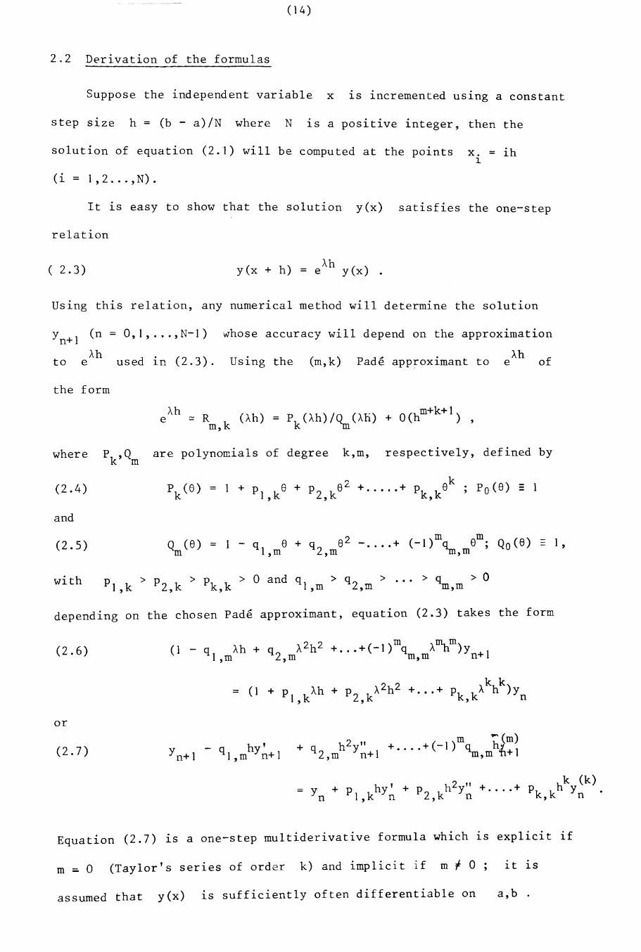
2.2 Derivation of the formulas
Suppose the independent variable x ~s incremented us~ng a constant
step s~ze h = (b - a)/N where N ~s a positive integer, then the
solution of equation (2.1) will be computed at the points x. = ihi.
(i = 1, 2 .•. ,N) •
It is easy to show that the solution y(x) satisfies the one-step
relation
( 2.3) Ahy(x + h) = e y(x).
Using this relation, any numerical method will determine the solution
whose accuracy will depend on the approximationYn+1 (n = O,I, ... ,N-I)
Ahto e used in (2.3).
the form
Using the (m,k) Pade approximant toAh
e of
where Pk,Qm are polynomials of degree k,m, respectively, defined by
(2.4)
and
P (e) = 1 + PI ke + p e 2 + ..... +k ,2,k
(2.5)
with
Q (e) = 1 - q e + q2 e 2 - .... + (_I)mq em; Qo(e) - 1,m I,m ,m "m,m
p > p > p > 0 and ql > q2 > ••• > ~ > 0l,k 2,k k,k ,m ,m ,m
depending on the chosen Pade approximant, equation (2.3) takes the form
(2.6)22m ~m(I - q Ah + q A h + ... +(-1) q A n)y 1
I,m 2,m m,m n+
or
(2.7) h 'y n+ 1 - q 1,m y n+ 1 + h 2 " ( l)m h(m)q2,m Yn+l + .... + - ~,m t+1
= y + PI khYn' + p h 2y" + .... +n, 2,k n
Equation (2.7) is a one-step multiderivative formula which is explicit if
m = 0 (Taylor's series of order k) and implicit if m; 0 it ~s
assumed that y(x) is sufficiently often differentiable on a,b
( 15)
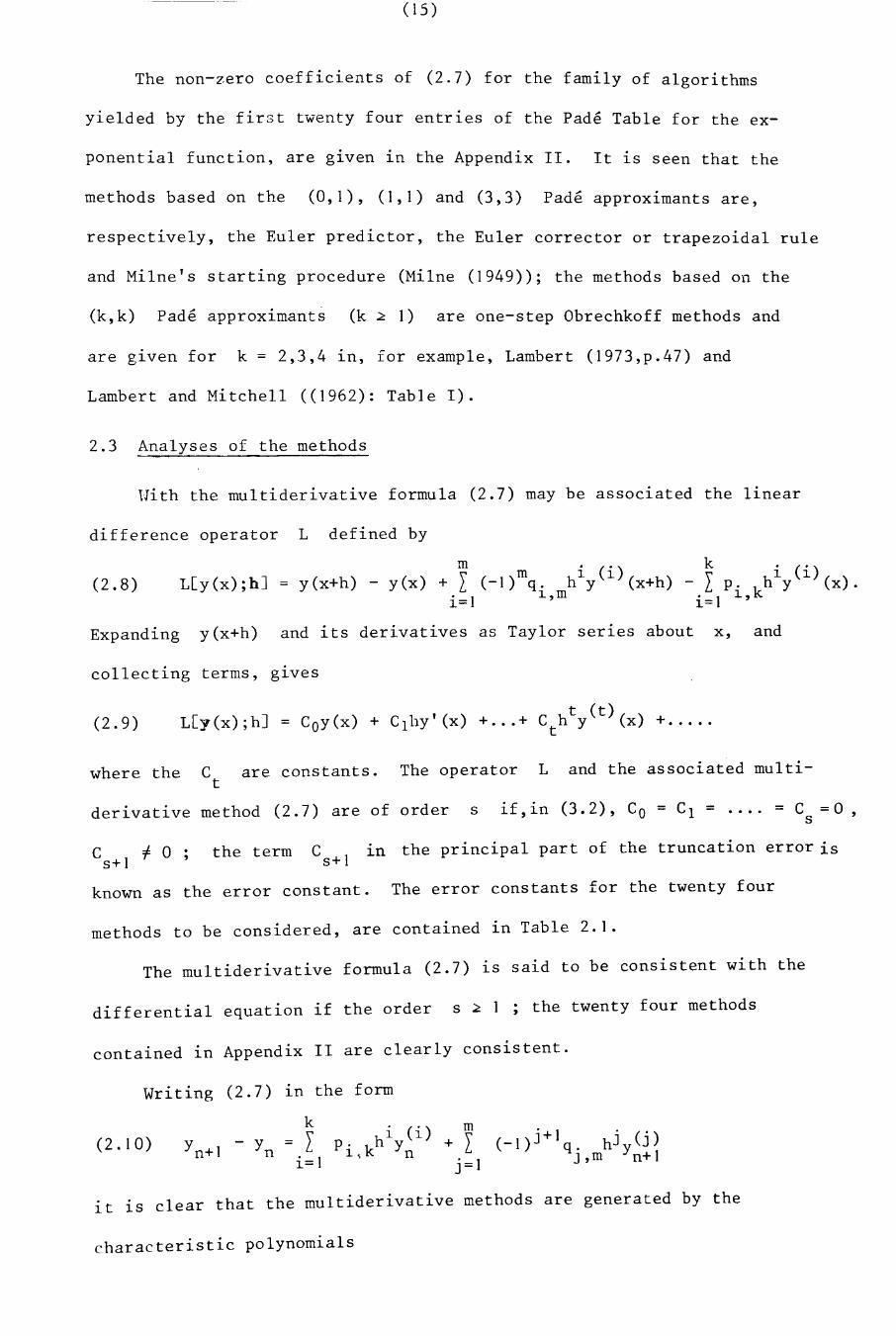
The non-zero coefficients of (2.7) for the family of algorithms
yielded by the first twenty four entries of the Pade Table for the ex-
ponential function, are given in the Appendix II. It is seen that the
methods based on the (0,1), (1,1) and (3,3) Pade approximants are,
respectively, the Euler predictor, the Euler corrector or trapezoidal rule
and Milne's starting procedure (Milne (1949»; the methods based on the
(k,k) Pade approximants (k ~ 1) are one-step Obrechkoff methods and
are glven for k = 2,3,4 1n, for example, Lambert (1973,p.47) and
Lambert and Mitchell «1962): Table I).
2.3 Analyses of the methods
'lith the multiderivative formula (2.7) may be associated the linear
difference operator L defined by
(2.8) LCy(x);hJ
Expanding y(x+h) and its derivatives as Taylor ser1es about x, and
collecting terms, glves
(2.9)t (t.)
LCy(x);hJ = Coy(x) + C1hy'(x) + ... + Cth Y (x) +.....
if,in (3.2), Co = C1 = •••. = C =0,s
The operator L and the associated multi-are constants.Ct
derivative method (2.7) are of order s
where the
C 1 f. °s+the term C In the principal part of the truncation error is
s+1
known as the error constant. The error constants for the twenty four
methods to be considered, are contained in Table 2.1.
The multiderivative formula (2.7) is said to be consistent with the
differential equation if the order s ~ 1 ; the twenty four methods
contained in Appendix II are clearly consistent.
(2.10)
Writing (2.7) 1n the form
k m= \ hi (i) + \
L Pi,k Yn Li= 1 j =1
it 1S clear that the multiderivative methods are generated by the
characteristic polynomials
(2.11)
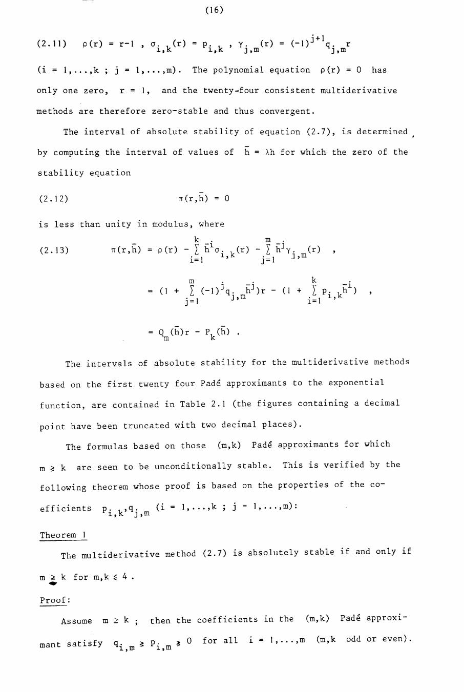
(16)
• 1per) = r-1 , cr. k(r) = p. k ,y. (r ) = (-OJ+ q. r
1, 1, J,m J,m
( i = 1, .•• ,k ,.' 1 )J = , ... ,m. The polynomial equation per) = 0 has
only one zero, r = 1, and the twenty-four consistent multiderivative
methods are therefore zero-stable and thus convergent.
The interval of absolute stability of equation (2.7), 1S determined
by computing the interval of values of
stability equation
-h = Ah for which the zero of the
(2.12)-
iT(r,h) = 0
1S less than unity 1n modulus, where
(2.13) iT(r,h) = per)k . m .\ -1 -J
- L h cr. k (r) - L h y. (r)i=l 1, j=l J ,m
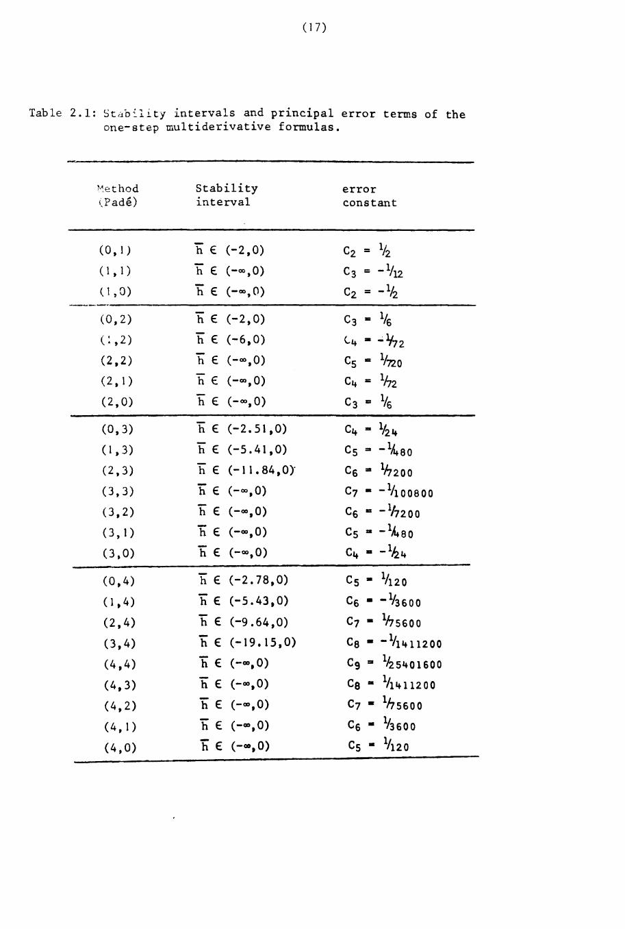
The intervals of absolute stability for the multiderivative methods
based on the first twenty four Pade approximants to the exponential
function, are contained in Table 2.1 (the figures containing a decimal
point have been truncated with two decimal places).
The formulas based on those (m,k) Pade approximants for which
m ~ k are seen to be unconditionally stable. This is verified by the
following theorem whose proof is based on the properties of the co-
efficients p. k,q. (i = 1, ... ,k; j = l, ... ,m):1, J , m
Theorem
The multiderivative method (2.7) is absolutely stable if and only if
m ~ k for m,k ~ 4 ...Proof:
Assume m ~ k then the coefficients in the (m,k) Pade approx1-
mant satisfy for all i = l, ... ,m (m,k odd or even).
(17)
Table 2.1: Stao:lity intervals and principal error terms of theone-step multiderivative formulas.
~~"ethod
(Pade)Stabilityinterval
errorconstant
- (-2,0) V2(0, I ) h E C2 =( I t 1) h E (-00 t 0) C3 = _1II2
(1,0) h E (-00,0) C2 = _1/2--_._...
(0,2) h E (-2,0) C3 -= 1/6
(: ,2) h E (-6,0) (..4 - ~lf,2
(2,2) h E (-00,0) Cs 0= 1/720
(2,1) h E (-00,0) C4 = 1h2
(2,0) h E (-00,0) C3 = 1/6
(0,3) h E (-2.51,0) C4 ::I 1/2 4
( 1,3) hE (-5.41,0) Cs = -11480
(2,3) h E (-1 1. 84,0)" C6 • Ih200
(3,3) hE (-00,0) C7 - _1II ooaoo
(3,2) h E (-00,0) C6 II: -117200
(3,1) h E (-00,0) Cs • _1A.ao
(3,0) h E (-00,0) C4 • _1&4
(0,4) hE (-2.78,0) Cs • lII20
(1,4) hE (-5.43,0) C6 • _1/36 00
(2,4) hE (-9.64,0) C7 • 1hs600- (-19.15,0) C8 • - lii 4 11200(3,4) h E
(4,4) hE (-00,0) C9 • 1/2 54 0 1 6 00
(4,3) hE (-00,0) Ce • 111411200
(4,2) hE (-00,0) C7 • 1hs600
(4,1) h E (-00,0) C6 • 1/36 0 0
(4,0) hE (-00,0) Cs - 1/120
(I8)
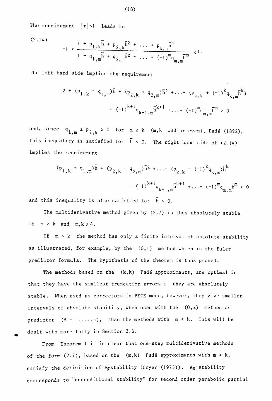
The requirement Irl<1 leads to
(2.14 )
-1 < -- q h +
I ,m< 1 •
The left hand side implies the requirement
2 + (PI,k - ql,m)h + (P2,k + q2,m)h2 +... + (Pk,k + (-1)kqk,mhk)
+ (_I)k+l h-k+ I (,m:-Illqk+l,m +... + -I) ~,mh > 0
and, S1.nce q. ~ p. k 2 0 for m ~ k1.,m 1.J
this inequality satisfied -1.S for h < O.
implies the requirement
(m,k odd or even), Pade (1892),
The right hand side of (2.14)
(Pk,k - (_I)kq )hkk,m
_ (_I)k+l h-k+ 1 m-mqk+1,m + ... - (-1) ~,mh < 0
-and this inequality is also satisfied for h < O.
The multiderivative method given by (2.7) 1.S thus absolutely stable
if m2k and m,k~4.
If m < k the method has only a finite interval of absolllte stability
as illustrated, for example, by the (0,1) method which is the Euler
predictor formula. The hypothesis of the theorem is thus proved.
The methods based on the (k,k) Pade approximants, are optimal l.n
that they have the smallest truncation errors; they are absolutely
stable. \fhen used as correctors in PECE mode, however, they give smaller
intervals of absolute stability, when used with the (0,£) method as
predictor (£ = 1, ... ,k), than the methods with m < k. This will be
dealt with more fully in Section 2.6.
From Theorem 1 it is clear that one-step multiderivative methods
of the form (2.7), based on the (m,k) Pade approximants with m ~ k,
satisfy the definition of ~stability (Cryer (1973)). Ao-stability
corresponds to "unconditional stability" for second order parabolic partial
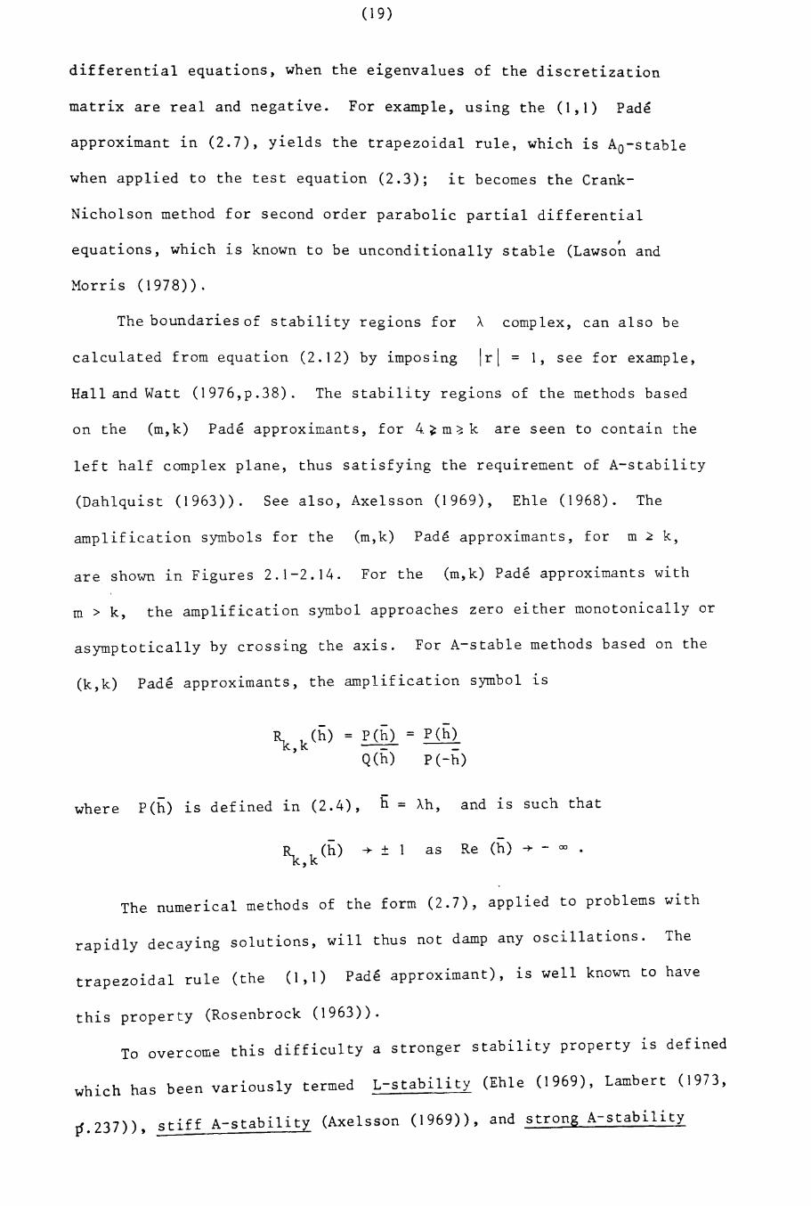
(19)
differential equations, when the eigenvalues of the discretization
matrix are real and negative. For example, using the (1,1) Pade
approximant in (2.7), yields the trapezoidal rule, which ~s Ao-stable
when applied to the test equation (2.3); it becomes the Crank-
Nicholson method for second order parabolic partial differential
equations, which is known to be unconditionally stable (Lawso~ and
Morris (1978».
The boundaries of s tabili ty r eg i on s for A comp lex, can also be
calculated from equation (2.12) by imposing Ir\ = 1, see for example,
Hall and Watt (1976,p.38). The stability regions of the methods based
on the (m, k ) Pade approximants, for 4. ~ m~ k are seen to contain the
left half complex plane, thus satisfying the requirement of A-stability
(Dahlquist (1963». See also, Axelsson (1969), Ehle (1968). The
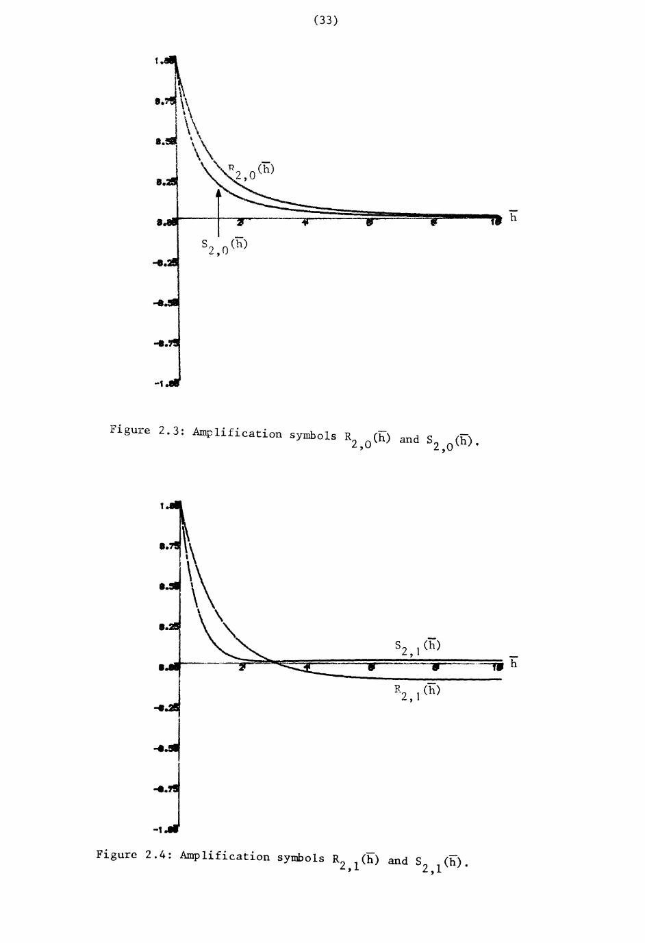
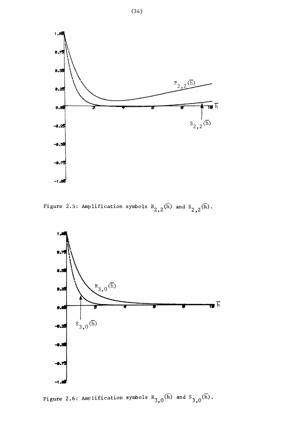
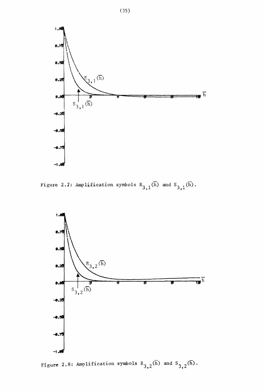
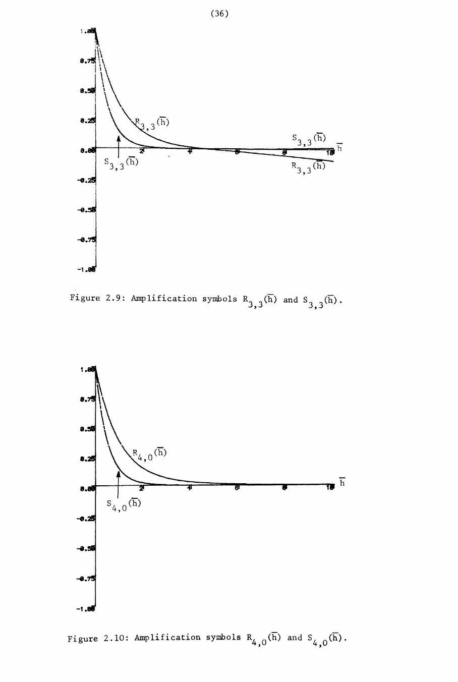
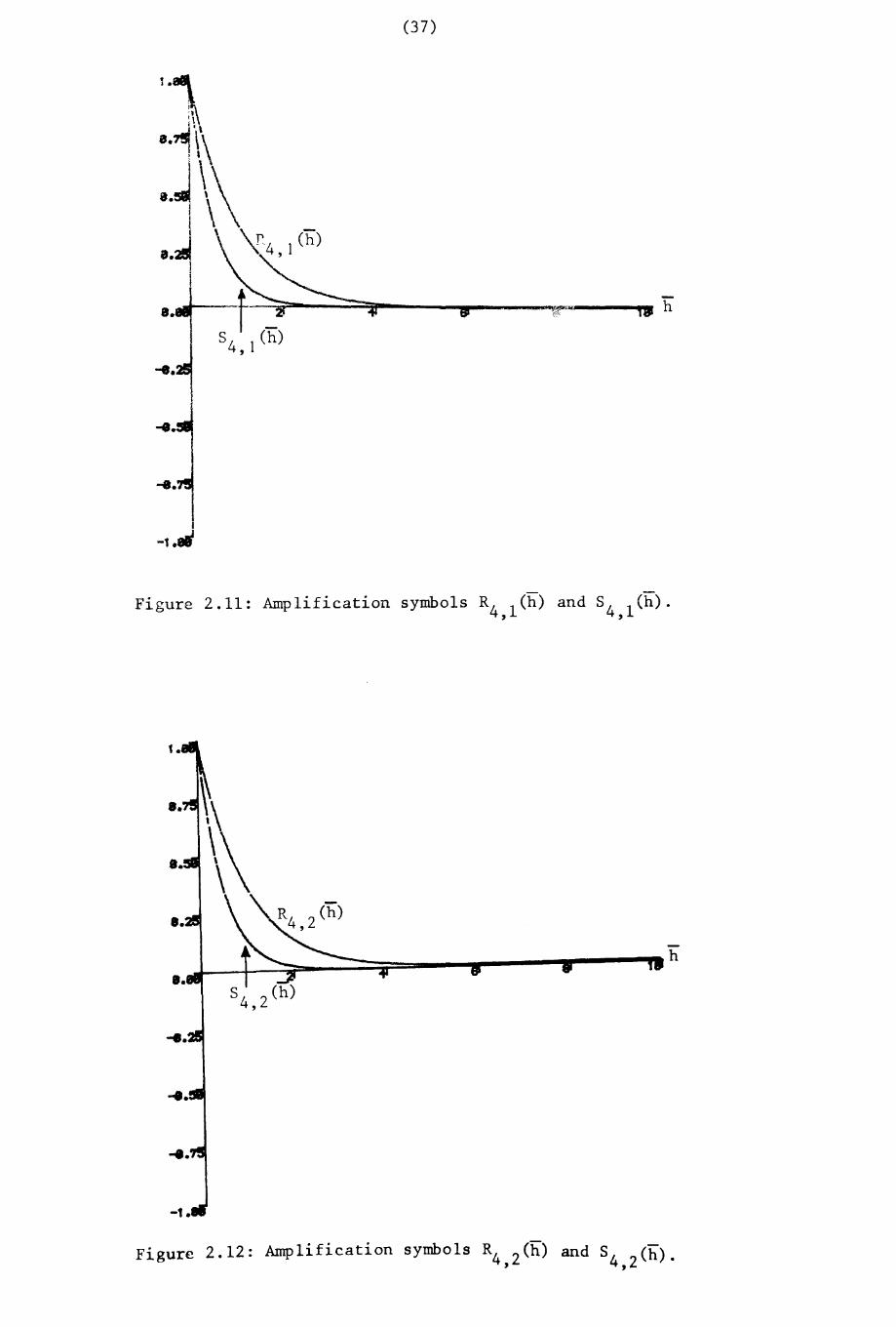
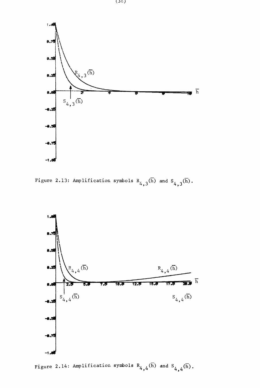
amplification symbols for the (m,k) Pade approximants, for m ~ k,
are shown in Figures 2.1-2.14. For the (m,k) Pade approximants with
m > k, the amplification symbol approaches zero either monotonically or
asymptotically by crossing the axis. For A-stable methods based on the
(k, k ) Pade approximants, the amplification symbol ~s
-l\ k(h) = P(h) = P (h),
Q(h)-
PC-h)
where P(h) ~s defined ~n (2.4), ii = Ah, and ~s such that
- -l\,k(h) + + as Re (h) + - OJ .
The numerical methods of the form (2.7), applied to problems with
rapidly decaying solutions, will thus not damp any oscillations. The
trapezoidal rule (the (1,1) Pade approximant), is well known to have
this property (Rosenbrock (1963».
To overcome this difficulty a stronger stability property is defined
which has been variously termed L-stability (Ehle (1969), Lambert (1973,
~.237», stiff A-stability (Axelsson (1969», and strong A-stability
(20)
(Chipman (1971), Axelsson (1972)). Following Ehle (1969), Lambert
(1973, p.236) has made the following definition of L-stability:
Definition: A one-step numerical method is said to be L-stable if
it is A-stable and, In addition, when applied to the scalar test
equation y' = Ay , A a complex constant with Re A < 0 it yields
Yn+] = R(hA)Yn' where IR(hA) I + 0 as Re(hA) + - 00
One-step multiderivative methods of the form (2.7) yielded by
employing the (m,k) Pade approximants, for m > k, are thus
L-stable; this is also clear from the corresponding Figures. It lS
noted that the amplification symbols for L-stable methodE approach
zero rapidly as soon as the degree of m increases compared to that
of k, and hence oscillations will be damped quickly by employing
higher order Pade approximants for which m > k. The behaviour of
higher order (m,O) Pade approximants and corresponding (m,k) Pade
approximants, for m > k, will be discussed in Chapter 3 for parabolic
partial differential equations in which discontinuities exist between
initial and boundary values.
(21)
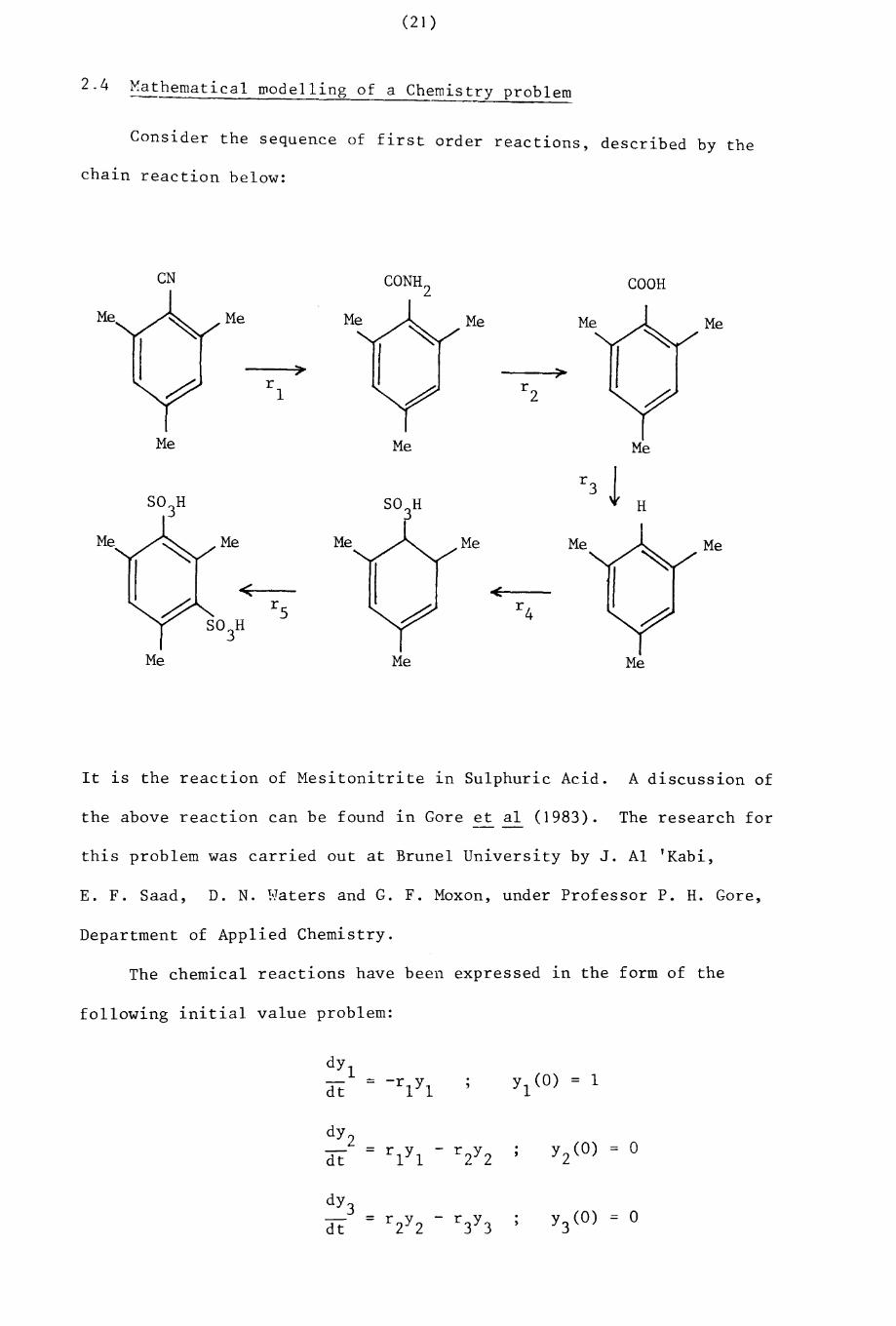
2.4 Mathematical IDodelling of a Chemistry problem
Consider the sequence of first order reactions, described by the
chain reaction below:
CN CONH2 COOH
Me Me Me Me
)0- ~r r
21
Me Me Me
r3 JS03H H
Me Me Me Me Me
<: <r S r 4
S03H
Me Me Me
It is the reaction of Mesitonitrite in Sulphuric Acid. A discussion of
the above reaction can be found in Gore et al (1983). The research for--
this problem was carried out at BruneI University by J. Al 'Kabi,
E. F. Saad, D. N. Waters and G. F. Moxon, under Professor P. H. Gore,
Department of Applied Chemistry.
The chemical reactions have been expressed In the form of the
following initial value problem:
dYlYl (0) = 1- = -r
l Yldt
dY 2 rl Yl
- r2Y2
y2(0)
= 0=dt
dY3 r2Y2
- r3Y3
y3(O)
= 0=dt
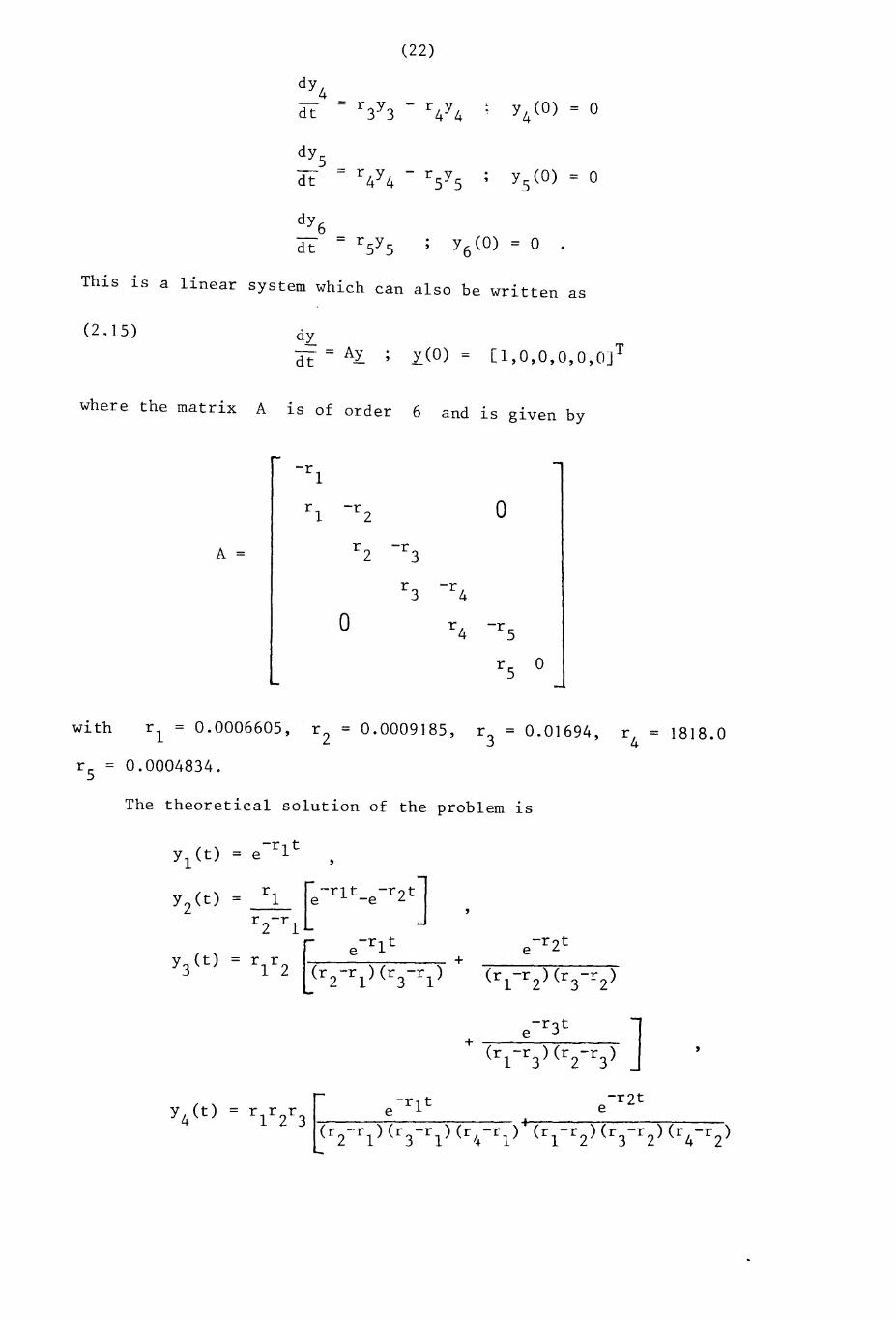
(22)
dY4- = r
3Y3- r
4Y4dt
dyS = r
4Y4- r
5y
Sdt
This is a linear system which can also be written as
(2.15) dy
dt yeo) = [l,O,O,O,O,OJ T
where the matrix A lS of order 6 and lS given by
-r1
r1
-r a2
r 2 -rA = 3
r3
-r4
a r4 -r
5
r 5 °with r 1 = 0.0006605, r 2 = 0.0009185, r
3= 0.01694, r
4= 1818.0
r = 0.0004834.5
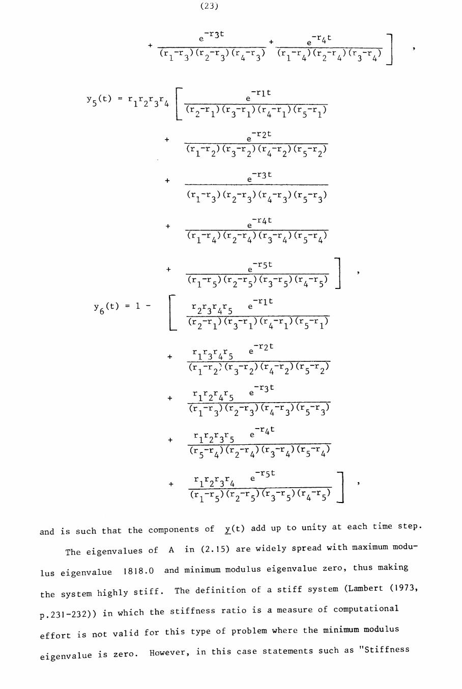
The theoretical solution of the problem lS
Y1 (t) = e-r 1t ,
Y2(t) r r-qt -rztJ= 1 e -er
2-r 1-r2 t[< e-rl t e
Y3(t) = r r +1 2 (r -r )(r -r ) (r1-r2) (r3- r 2)2 1 3 1
e-r 3t ]+ ,(r1-r3)
(r2-r3)
~ -rlt-r2t
Y4(t)e= r
1r2r3e
r 1)' (r1-r2)(r3-r2)(r4(r2-r1)(r3-r1)(r4 r2)
(23)
,+ +~--"""""----:-~--- -;~-~~----.,----
-rlte
r l)(r3-r l)(r
4-rl)(rS-r
l)
+-rzt
e
+-r3 t
e
+
+
[+
+
+
+
and ~s such that the components of y(t) add up to unity at each time step.
The eigenvalues of A in (2.15) are widely spread with maximum modu-
Ius eigenvalue 1818.0 and minimum modulus eigenvalue zero, thus making
the system highly stiff. The definition of a stiff system (Lambert (1973,
p.231-232)) in which the stiffness ratio ~s a measure of computational
effort is not valid for this type of problem where the minimum modulus
eigenvalue is zero. However, in this case statements such as "Stiffness

(24)
occurs when stability rather than accuracy dictates the choice of step
length", are preferred (Lambert (1980,p.21).
To compute the solution of the system (2.15), it can easily be shown
that (2.15) satisfies the equation (2.3), which can be written as
(2.16) y(t+£) = exp (£A)y(t) ,
where £ r.s a convenient time step.
The fourth order, A-stable method based on the (2,2) Pade approx~
mant (Appendix II) may be used to determine the solution from (2.16). The
numerical results were calculated us~ng single precision arithmetic and the
sum of the six components of I.(t), t = 0(500)5000, was found to be unity
to ten decimal places. The numerical results are given in the Table 2.2.
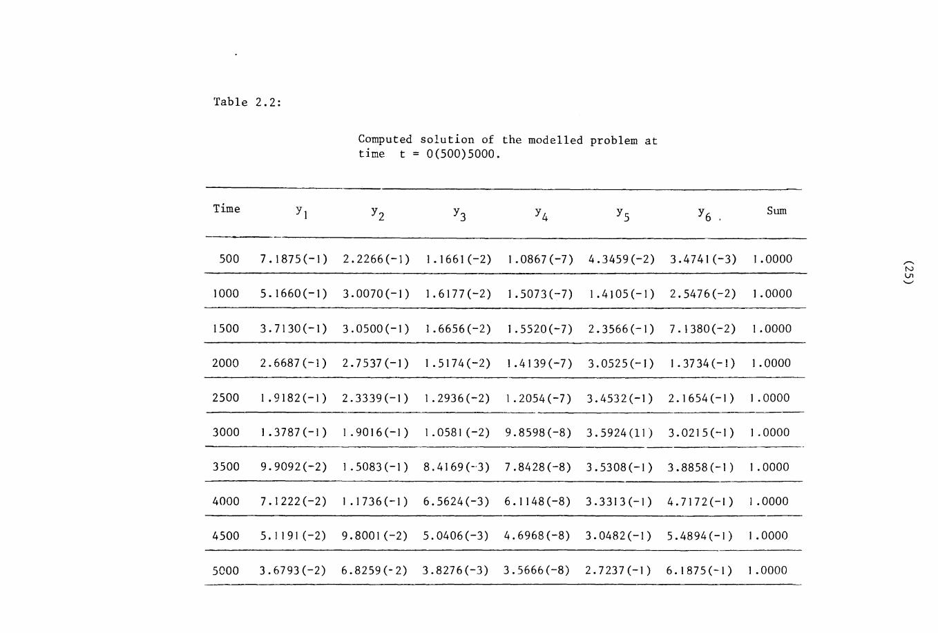
Table 2.2:
Computed solution of the modelled problem attime t = 0(500)5000.
Time YI Y2 Y3 Y4 Y5 Y6 . Sum
500 7.1875(-1 ) 2.2266(-1) 1.1661 (-2) 1.0867 (-7) 4.3459(-2) 3.4741(-3) I .0000 ,........NlJl'-"
1000 5.1660(-1) 3.0070(-1) 1.6177(-2) 1.5073(-7) 1. 41 05 (-I) 2.5476(-2) I .0000
1500 3. 7130 (-I) 3.0500(-1) 1.6656(-2) 1.5520(-7) 2.3566(-1) 7.1380(-2) I .0000
2000 2.6687(-1) 2.7537(-1) 1.5174(-2) I .4139 (-7) 3.0525(-1) 1.3734(-1) I .0000
2500 1.9182(-1 ) 2.3339(-1) 1.2936(-2) 1.2054(-7) 3.4532(-1) 2.1654(-1) I .0000
3000 1.3787(-1) 1.9016 (-I ) 1.0581 (-2) 9.8598(-8) 3.5924(11) 3.0215(-1) I .0000
3500 9.9092(-2) 1.5083 (-I ) 8 . 4169 (_.3) 7.8428(-8) 3.5308(-1) 3.8858(-1) 1.0000
4000 7.1222(-2) 1.1736(-1) 6.5624(-3) 6. I 148(-8) 3.3313(-1) 4.7172(-1) I . 0000
4500 5.1191(-2) 9.8001 (-2) 5.0406(-3) 4.6968(-8) 3.0482(-1) 5.4894(-1) 1. 0000
5000 3.6793(-2) 6.8259(-2) 3.8276(-3) 3.5666(-8) 2. 7237 (-I ) 6.1875(-1) 1. 0000
(26)
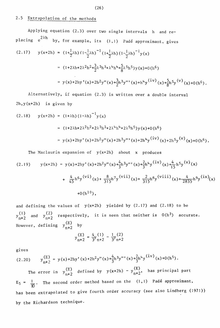
2.5 ~xtrapolation of the methods
Applying equation (2.3) over two single intervals hand re
2Ahplacing e by, for example, its (l~l) Pade approximant, glves
(2.17)
Alternatively, if equation (2.3) 1S written over a double interval
2h,y(x+2h) is given by
(2.18) y(x+2h) = (I+Ah)(I-Ah)-ly(x)
The Maclaurin expanS10n of y(x+2h) about x produces
(2.19)
+ ~h6 (vi) () ~h7 (vii) () ~h8 (viii) () 4 h 9 (ix)( )45 y x + 315 Y x + 315 Y x + 2835 Y x
and defining the values of y(x+2h) yielded by (2.17) and (2.18) to be
Y( 2) respectively,n+2and
However, defining(E)
Yn+2 by
it is seen that neither is o(h 3) accurate.
(2.20)
The error 1n(E)
Yn+2defined by
(E)y(x+2h) - Yn+2' has principal part
ES = The second order method based on the (I , I) Pade approximant,
has been extrapolated to glve fourth order accuracy (see also Lindberg (1971»
by the Richardson technique.
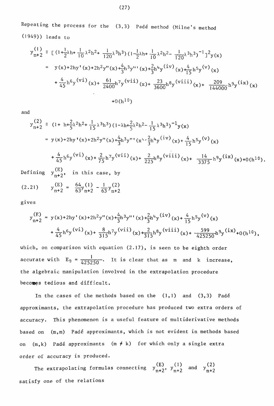
(27)
Repeating the process for the (3~3) Pade method (Milne's method
(1949» leads to
0)Yn+ 2 -
=
and
(2)Yn+ 2 -
[(l+21Ah+ 110A2h2+ _1_A3h3)(I~Ah+_l_A2h2__1_A3h 3)-IJ2 ( )120 2 10 120 Y x
y (x)+2hy' (x)+2h2y" (x)~h 3y'" (x)2h4y(iv) (x)~hS (v ) ( )3 3 15 Y x
+ !:-h6 (vi) () 61 7 (vii) 23 8 (viii) 209 (.)45 Y x + 2400h y (x)+ h - () h 9 t.x ( )3600 Y x + 144000 Y x
+ ~h6y(vi) (x)+ 2-h 7y (v i i ) (x)+ ~8y(viii)( )+45 75 225 x
Defining
(2.21)
g~ves
(E)Yn+2'
(E)Yn+2 =
~n this case, by
(E)Yn+2 = y(x)+2hy' (x)+2h2Y"(x)~3y'"(x)A4y(iv) (x)+ !:-hSy(v) (x)
3 3 15
+ ~h6 (vi) ( )+ ~h7 (vii) () 2 h 8 (viii) () 599 h 9 (ix) 0(h 1 0 )45 y x 315 Y x +m y x + 425250 Y + ,
which, on compar~son with equation (2.17), is seen to be eighth order
accurate with 1E9 = 425250 It is clear that as m and k .
~ncrease,
the algebraic manipulation involved in the extrapolation procedure
beco~s tedious and difficult.
In the cases of the methods based on the (1,1) and (3,3) Pade
approximants, the extrapolation procedure has produced two extra orders of
accuracy. This phenomenon is a useful feature of multiderivative methods
based on (m,m) Pade approximants, which is not evident in methods based
on (m,k) Pade approximants (m, k) for which only a single extra
order of accuracy is produced.
The extrapolating formulas connecting
satisfy one of the relations
(E) (J )Yn+2' Yn+2 and
(2)Yn+2
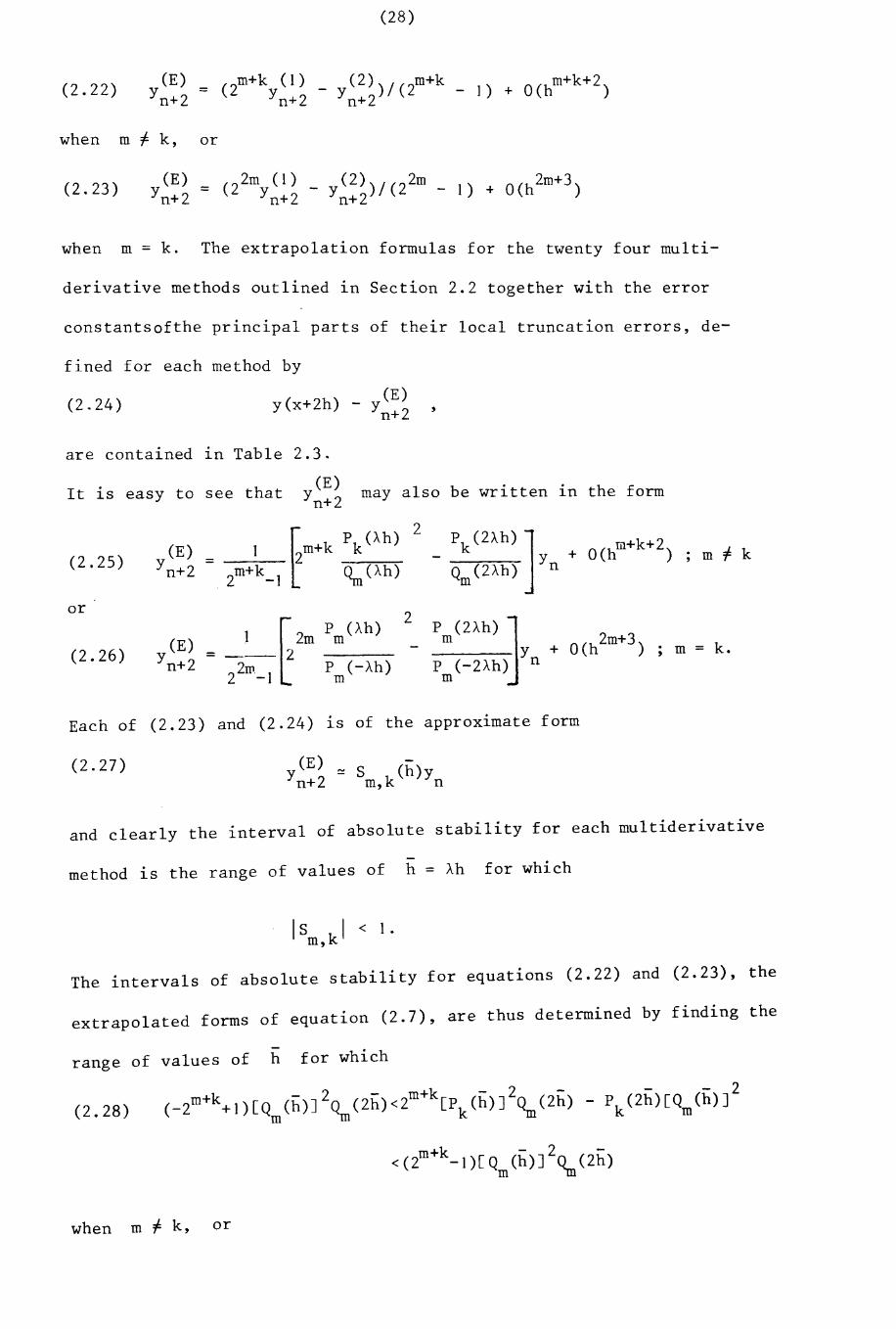
(28)
(2.22)(E) = (2m+k (I) _ (2))/(2ID+k _ ]) + O(hm+k+ 2)
Yn+2 Yn+2 Yn+2
when m :f k, or
(2.23) (E) = (22m (1) (2))/(22m - 1) + O(h 2m+3)
Yn+ 2 Yn+2 Yn+2
when m = k. The extrapolation formulas for the twenty four multi-
derivative methods outlined in Section 2.2 together with the error
constantsofthe principal parts of their local truncation errors, de-
fined for each method by
(2.24)(E)
y(x+2h) - Yn+2 '
are contained In Table 2.3.
It is easy to see that(E)
Y may also be written In the formn+2
Pk(Ah)2
Pk (ZAh) J + 0 (hm+k+2(2.25)
(E) I Em+k
Yn+2 = Q (2Ah) Yn )2m+k_1 ~(Ah) m
or
) ~ Zm Pm (Ah)2
P (2Ah) j(E) _ m Y + 0 (h2m+3)
(2.26) Yn+2 = 22m_1
2 Pm(-Ah) P (-2Ah) nm
Each of (2.23) and (2.24) lS of the approximate form
m :f k
m = k.
(2.27) (E)Yn +2 ::: S k(h)ym, n
and clearly the interval of absolute stability for each multiderivative
-method is the range of values of h = Ah for which
Is k l < 1.m,
The intervals of absolute stability for equations (2.22) and (2.23), the
extrapolated forms of equation (2.7), are thus determined by finding the
-range of values of h for which
(2.28) (_2m+k+l)[Qm(h)]2~(2h)<2m+k[Pk(h)]2~(2h)- Pk(2h)[Qm(h)]2
«2m+k_I)[Qm(h)J2~(2h)
when m:f k, or
(2.29)
(29)
2m - 2 - 2 2 2(-2 +])[P (-h)J P (-2h) <2 m[p (h)J P (-2h)-P (2h)[P (-h)J
rn rn rr 1"'") rn rn
when rn = k.
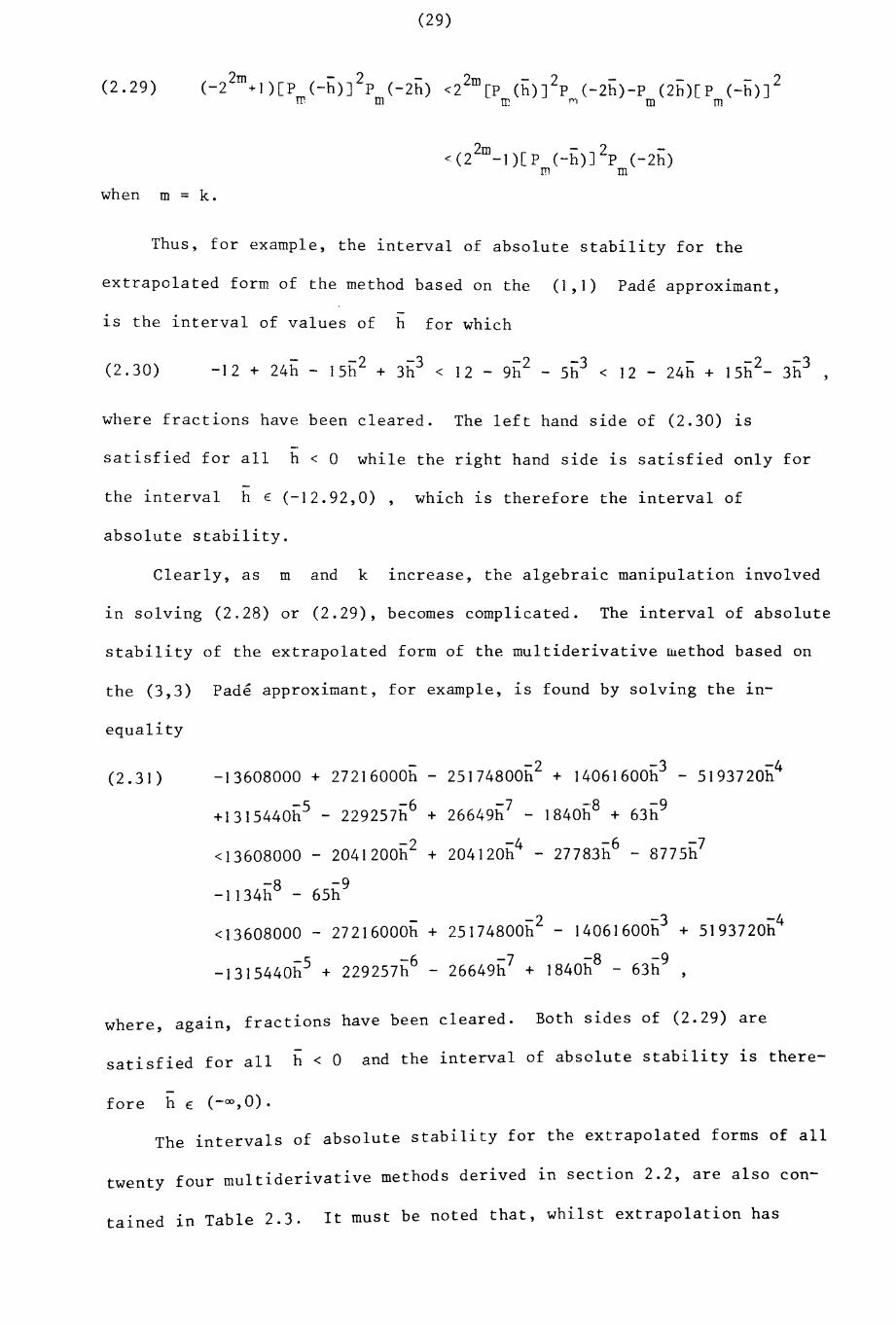
Thus, for example, the interval of absolute stability for the
extrapolated form of the method based on the (],]) Pade approximant,
is the interval of values of -h for which
(2.30)
where fractions have been cleared. The left hand side of (2.30) 1S
-satisfied for all h < 0 while the right hand side is satisfied only for
-the interval h E (-]2.92,0), which is therefore the interval of
absolute stability.
Clearly, as m and k 1ncrease, the algebraic manipulation involved
1n solving (2.28) or (2.29), becomes complicated. The interval of absolute
stability of the extrapolated form of the multiderivative lliethod based on
the (3,3) Pade approximant, for example, is found by solving the in-
equality
(2.31) -13608000 + 27216000h - 25174800h2
+ 1406]600h3
- 5193720h4
+]315440h5 - 229257h6 + 26649h7
- ]840h8
+ 63h9
<13608000 - 204]200h2
+ 204]20h4
- 27783h6
- 8775h7
-1134h8 - 65h9
<13608000 - 27216000h + 25174800h2
- ]406]600h3
+ 5193720h4
-]315440h5 + 229257h6
- 26649h7
+ 1840h8
- 63h9
where, aga1n, fractions have been cleared. Both sides of (2.29) are
satisfied for all h < 0 and the interval of absolute stability is there-
-fore h E (-00,0).
The intervals of absolute stability for the extrapolated forms of all
twenty four multiderivative methods derived in section 2.2, are also con-
tained in Table 2.3. It must be noted that, whilst extrapolation has
(30)
improved accuracy, this has often been at the expense of a decreased
interval of absolute stability. This is particularly so with the (0,1)
and (1,1) Pade methods which are, of course, the Euler predictor
formula and the Euler corrector formula (the trapezoidal rule)
respectively. The extrapolated form of the (1,1) method does not
satisfy Theorem 1 which, therefore, does not hold for the extrapolation
formulas. However, it is seen from equation (2.25) that the
extrapolation of L-stable methods based on (m,k) Pade approximants with
m> k , satisfies the condition of L-stability. Thus, the extrapolation
of L-stable methods of the form (2.7) based on (2.25), is L-stable
since the degree of the denominator in
degree of the numerator for m> k .
R k(~)m, is greater than the
The amplification symbols for the extrapolated methods are also
shown in Figures 2.1 - 2.14. It is seen that the amp lification symbols
of the extrapolated methods based on the (m,k) Pade approximants
for m> k, approach zero faster than those of the methods themselves,
thus damping oscillations more quickly.
(31)
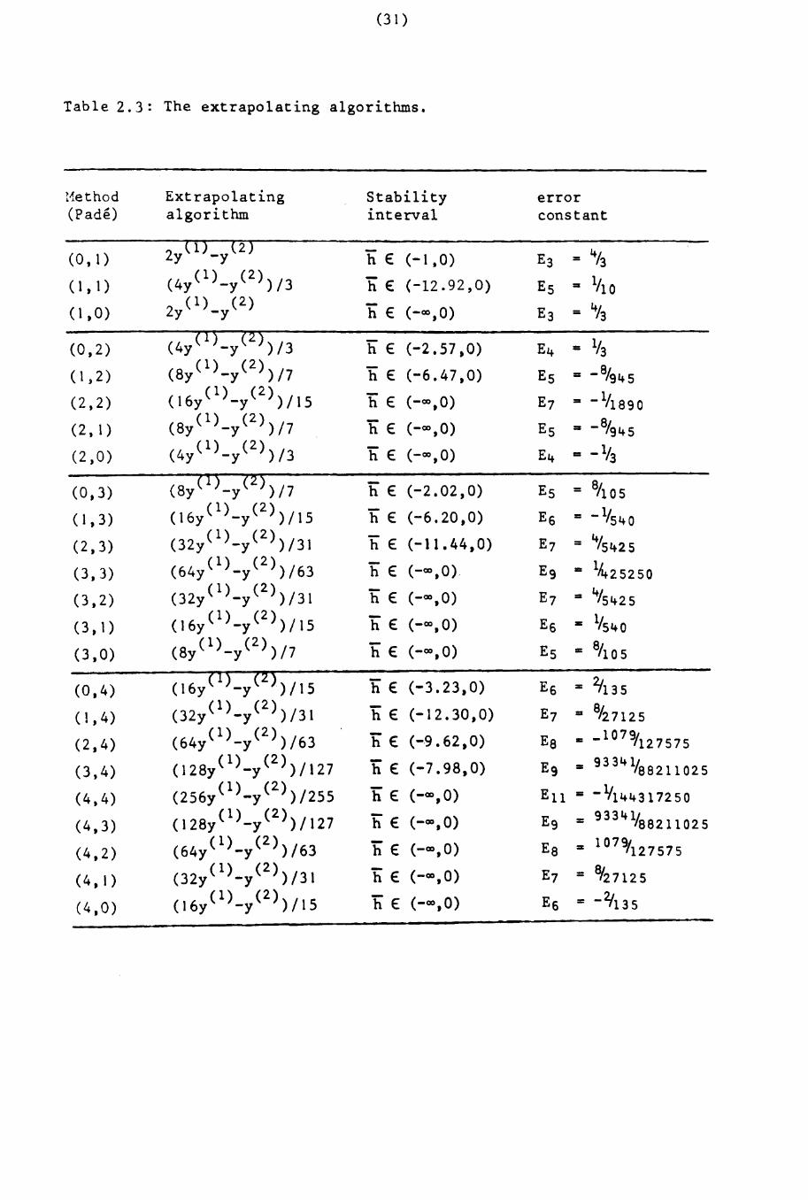
Table 2.3: The extrapolating algorithms.
!1ethod Extrapolating Stability error(Pade ) algorithm interval constant
2 (1) (2)(0, 1) h E (-1,0) = '+/3Y -y E3
( 1, 1) (4y(1)_y(2»/3 hE (-12.92,O) E5 = 1/10( 1, 0) 2y(1) _y (2) hE (-00,0) E3 = '+1)
(0,2) (4y(1)_y(2»/3 h E (-2.57,0) E,+ = 1/3( 1,2) (8y(1)_y(2»/7 h E (-6.47,0) E5 = _8/9,+5(2,2) (16y(1)_y(2»/15 hE (-00,0) E7 = -III 890
(2, 1) (8y(1)_y(2»/7 hE (-00,0) E5 = _8/g,+ 5
(2,0) (4y(1)_y(2»/3 h E (-00, 0) E,+ = _1/3
(0,3) (8y(1)_y(2»/7 liE (-2.02,0) E5 = 8/105
( 1,3) (16y(1)_y(2»/15 liE (-6.20,0) E6 = _1/5,+ 0
(2,3) (32y(1)_y(2»/31 h E (-11.44,0) E7 = '+/5425
(3,3) (64y(1)_y(2»/63 h E (-00,0) Eg = Ilt.2 52 50
(3,2) (32y(1)_y(2»/31 h E (-00,0) E7 = '+/5'+25
(3,1) ( 16y ( 1) _y (2) ) / 15 liE (-00,0) E6 .. lf51+ 0
(3,0) (8y(1)_y(2»/7 'hE (-00,0) E5 = 8II 05
(0,4) ( 16y( 1)_y (2» / 15 liE (-3.23,0) E6 = 2t1 3 5
(1,4) (32y(1)_y(2»/31 liE (-12.30,0) E7 = 8/27125
(2,4) (64y(1)_y(2»/63 'hE (-·9.62,0) E8 .. _107g/12 7575
(3,4) (128y(1)_y(2»/127 'hE (-7.98,0) Eg = 9331+ 1/8a211025
(4,4) (256y(1)_y(2»/255 'hE (-00,0) Ell = -¥11+1+317250
(4,3) (128y(1)_y(2»/127 'hE (-00,0) Eg = 9331+ 1/88211025
(4,2) (64y(1)_y(2»/63 liE (-00,0) Ea = 1079/127575
(4,1) (32y(1)_y(2»/31 'hE (-00,0) E7 = Bt27125
(4,0) (16y(1)_y(2»/15 liE (-00,0) E6 = -211 3 5
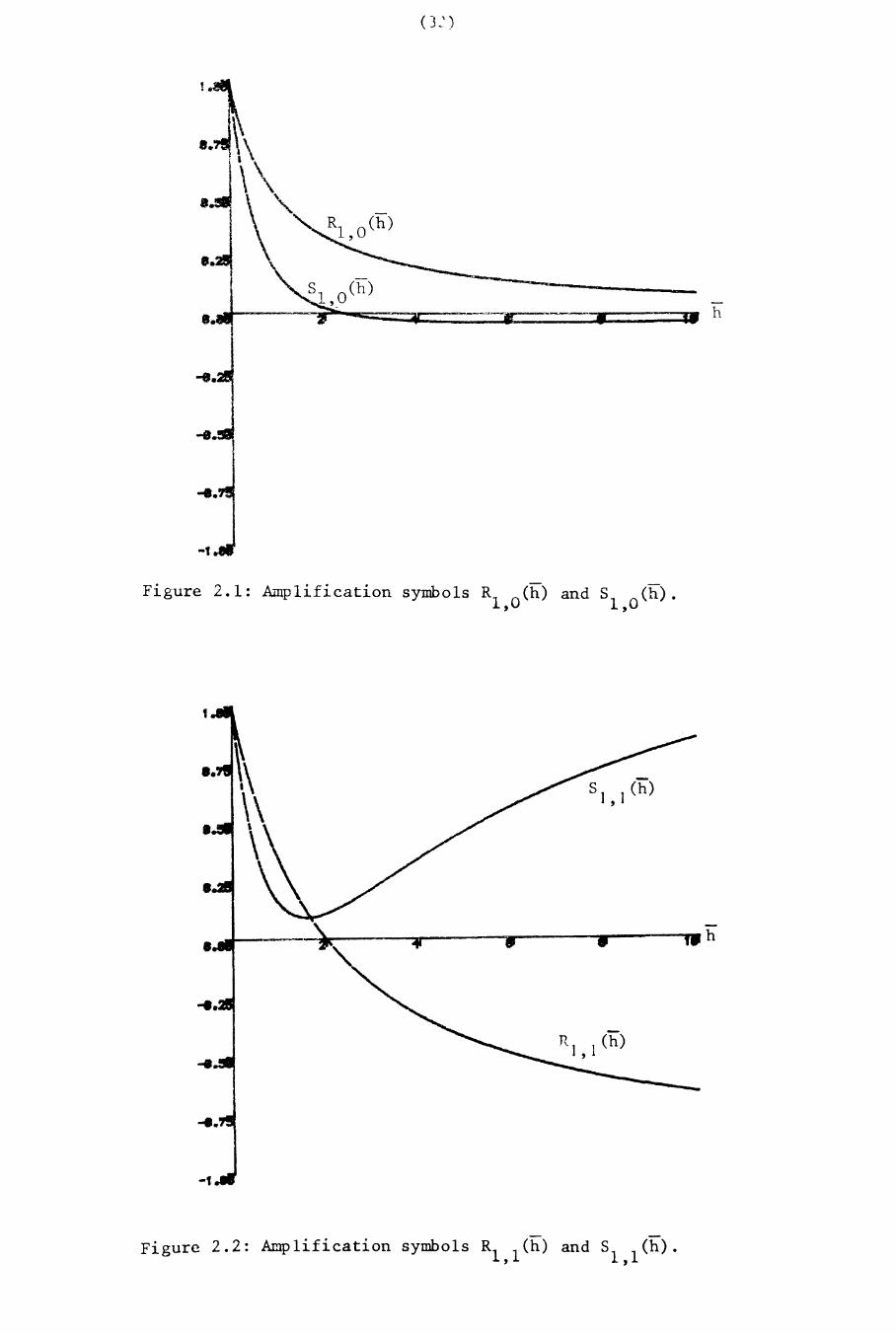
h
Figure 2.1: Amplification symbols R1,O(h) and Sl,o(h).
t
-L__~~--~--.-,_--......----..h
Figure 2.2: Amplification symbols R1,1(h) and Sl,l(h).
(33)
Figure 2.3: Amplification symbols R2
o(h) and 52 O(h)., ,
------. h
Figure 2.4: Amplification symbols RZ
l(h) and 52 l(h)., ,
(34)
Figure 2.5: Amplification symbols R2,2(h) and S2,2(h).
f
•• -L.-..l-:~r=--::::::===::::;;:=----....--.... h
...
-f
Figure 2.6: Amrlification symbols R3,O(h) and S3,O(h).
(35)
8.
8.
8.__-I-r--"';;;:==--:r-======ti~==~==='"h
,
-8.J'-8.
Figure 2.1: Amplification symbols R3,1(h) and S3,1 (h).
Figure 2.8: Amplification symbols R3,2(h) and S3,2(h).
(36)
R3 3(h),
Figure 2.9: Amplification symbols R3,3(h)
and 53,3(h).
~\
\\\R4, 0 (h)
-l--~::::;r=----=::::;r===__--.....--"m h
Figure 2.10: Amplification symbols R4 O(h) and 54 O(h)., ,
(37)
--=?---:=;p---.....oIl_--_~--_h
-t.ti
Figure 2.11: Amplification symbols R4,1(h) and S4,1(h).
1•
...L--l~:::;;=-======r==--.....-_..,,__..,.h
Figure 2.12: Amplification symbols R4,2(h) and S4,2(h).
(Jb)
8.
8.et--+,r--"=::~--1I"'--"''''-=====~1II
Figure 2.13: Amplification symbols R4,3(h) and S4,3(h).
Figure 2.14: Amplification symbols R4,4(h) and S4,4(h).
h
h
(39)
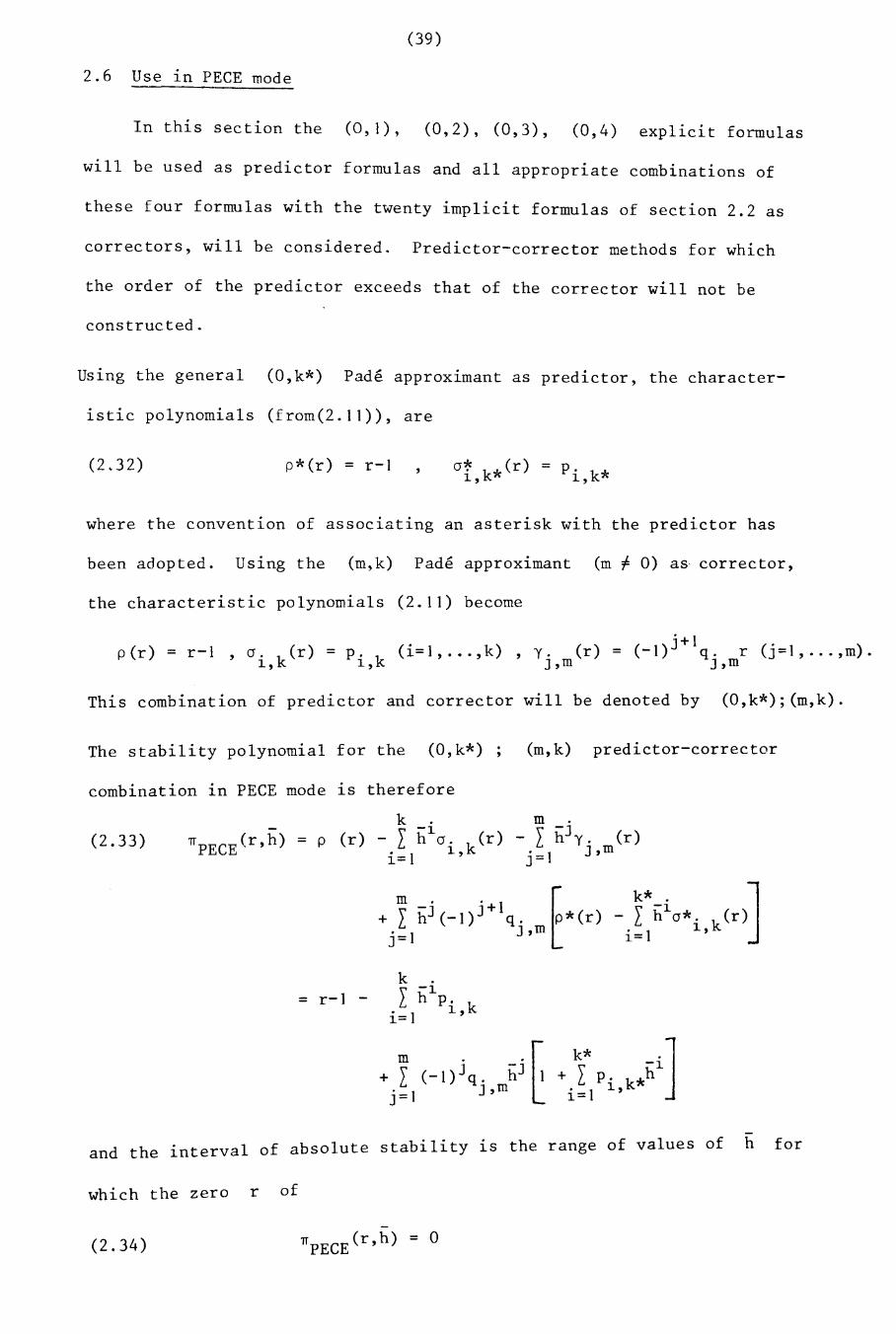
2.6 Use 1n PECE mode
In this s ec t i on the (0.1), (0 2) (0 3) (0 4) Li.c i t f 1' "", exp 1C1 ormu as
will be used as predictor formulas and all appropriate combinations of
these four formulas with the twenty implicit formulas of section 2.2 as
correctors, will be considered. Predictor-corrector methods for which
the order of the predictor exceeds that of the corrector will not be
constructed.
Using the general (O,k*) Pade approximant as predictor, the character-
istic polynomials (from(2.II)), are
(2.32) p*(r) = r-I o~ k*(r) = p. k*1, 1,
(2.33)
where the convention of associating an asterisk with the predictor has
been adopted. Using the (m,k) Pade approximant (m I- 0) as corrector,
the characteristic polynomials (2.11) become
. 1per) - r-I 0 (r) = p (i=I, ... ,k), y. (r ) = (-I)J+ q. r (J·=1, ... ,m).- ,. k . k1, 1, J,m J,m
This combination of predictor and corrector will be denoted by (O,k*);(m,k).
The stability polynomial for the (O,k*); (m,k) predictor-corrector
combination 1n PECE mode is therefore
k . m .-1 \' -J
TIpECE(r,h) = p (r) - L h o. k(r) - L h y. (r). 1 1, ·-1 J,m1= J-
k* . ]- L i?o*. (r ). 1 1, k1=
k .\' -1= r-l - L h p. k
• 1 1,1=
k* .J+ L p. k*l?
. 1 1,1=
and the interval of absolute stability 1S the range of values of h for
which the zero r of
(2.34)
(40)
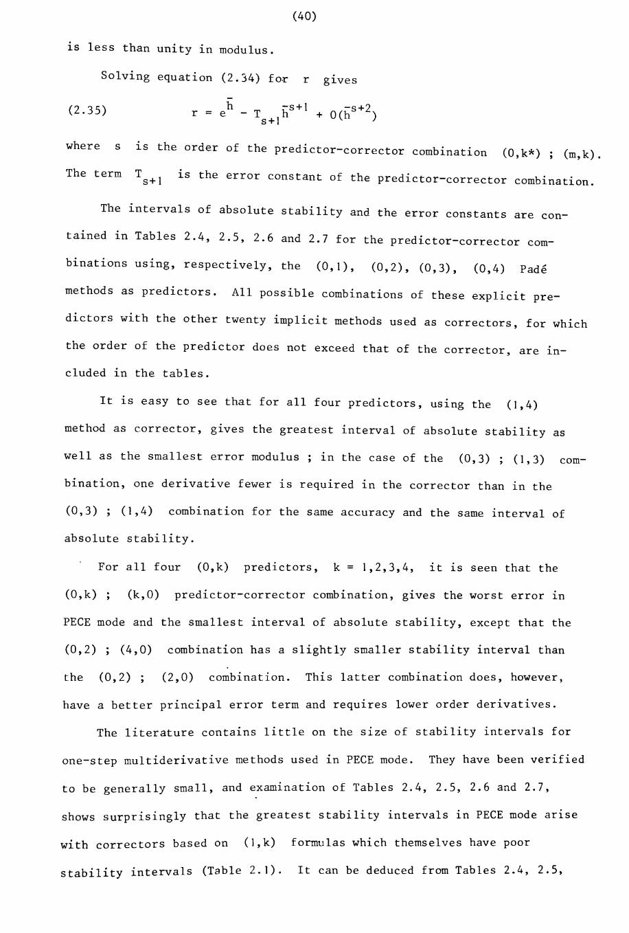
is less than unity 1n modulus.
Solving equation (2.34) for r g1ves
(2.35) r =-
eh _ T h-s +1 -s+2
+ O(h )s+ 1
where s is the order of the predictor-corrector combination (0 k*) (k), ; m, •
The term Ts+1 is the error constant of the predictor-corrector combination.
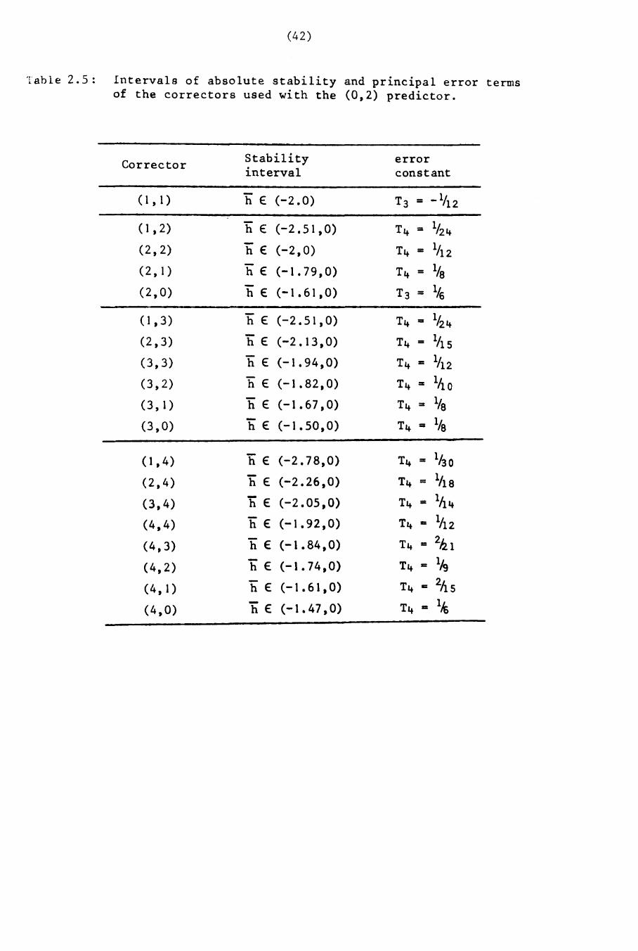
The intervals of absolute stability and the error constants are con-
tained in Tables 2.4, 2.5, 2.6 and 2.7 for the predictor-corrector com-
binations us i.ng , respectively, the (0,1), (0,2), (0,3), (0,4) Pade
methods as predictors. All possible combinations of these explicit pre-
dictors with the other twenty implicit methods used as correctors, for which
the order of the predictor does not exceed that of the corrector, are in-
eluded in the tables.
It is easy to see that for all four predictors, uS1ng the (1,4)
method as corrector, g1ves the greatest interval of absolute stability as
well as the smallest error modulus; in the case of the (0,3); (1,3) com-
bination, one derivative fewer is required in the corrector than in the
(0,3) ; (1,4) combination for the same accuracy and the same interval of
absolute stability.
For all four (O,k) predictors, k = 1,2,3,4, it 1S seen that the
(O,k); (k,O) predictor-corrector combination, gives the worst error 1n
PECE mode and the smallest interval of absolute stability, except that the
(0,2) ; (4,0) combination has a slightly smaller stability interval than
the (0,2); (2,0) combination. This latter combination does, however,
have a better principal error term and requ1res lower order derivatives.
The literature contains little on the size of stability intervals for
one-step multiderivative methods used in PECE mode. They have been verified
to be generally small, and examination of Tables 2.4, 2.5, 2.6 and 2.7,
shows surprisingly that the greatest stability intervals in PECE mode ar1se
with correctors based on (l,k) formulas which themselves have poor
stability intervals (Table 2.1). It can be deduced from Tables 2.4, 2.5,
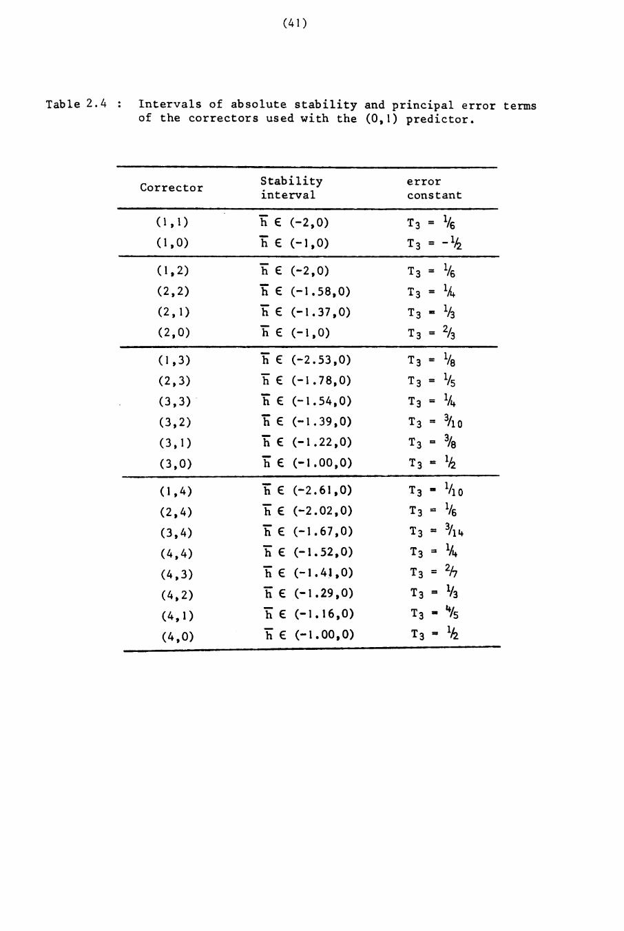
Table 2.4
(41 )
Intervals of absolute stability and principal error termsof the correctors used with the (0,1) predictor.
Corrector Stability errorinterval constant
( 1 , 1) h E (-2,0) T3 = 1/6(l,O) hE (-1,0) T3 = _1~
( 1,2) h E (-2,0) T3 = 1/6(2,2) hE (-1.58,0) T3 = lk(2, 1) hE (-1.37,0) T3 • 113
(2,0) h E (-1 ,0) T3 = 2/3
( 1,3) hE (-2.53,0) T3 = l/e(2,3) h E (-1.78,0) T3 = 1/5(3,3) . hE (-1.54,0) T3 = 1/4
(3,2) hE (-1.39,0) T3 = 3110
(3. 1) hE (-1.22,0) T3 = 3/e(3,0) hE (-1.00,0) T3 = Ih.
(l ,4) hE (-2.61,0) T3 • 1/10
(2,4) hE (-2.02,0) T3 = 1/6
(3,4) hE (-1.67,0) T3 = 3!I4
(4,4) hE (-1.52,0) T3 = 1/4
(4,3) hE (-1.41,0) T3 = 2h
(4,2) hE (-1.29,0) T3 = lf3
(4,1) hE (-1.16,0) T3 - 4/5
(4,0) h E (-1.00,0) T3 = liz
(42)
Table 2.5: Intervals of absolute stability and principal error termsof the correctors used with the (0,2) predictor.
Corrector Stability errorinterval constant
( 1 , 1) - (-2.0) T3 = -1/12h E
( 1 ,2) - (-2.51,0) Ih4h E T4 =- (-2,0) Ih2(2,2) h E T4 =- (-1.79,0) l/a(2, 1) h E T4 =
(2,0) h E (-1.61,0) T3 = 1/6
(I,3) h E (-2.51,0) T4 = 1/24
(2,3) hE (-2.13,0) T4 = 1115
(3,3) h E (-1.94,0) T4 = 1/12
(3,2) h E (-1.82,0) T4 =- lAo(3, 1) h E (-1.67,0) T4 =- l/a
(3,0) hE (-1.50,0) T4 = l/a
(1,4) hE (-2.78,0) T4 = 1130
(2,4) h E (-2.26,0) T4 = lila(3,4) h E (-2.05,0) T4 = 1114
(4,4) h € (-1.92,0) T4 = 1112
(4,3) h E (-1.84,0) Tit = 2hl
(4,2) h E (-1.74,0) T4 1:1 1/9
(4, 1) h E (-1.61,0) T4 1:1 2115
(4,0) h € (-1.47,0) T4 = 1,t
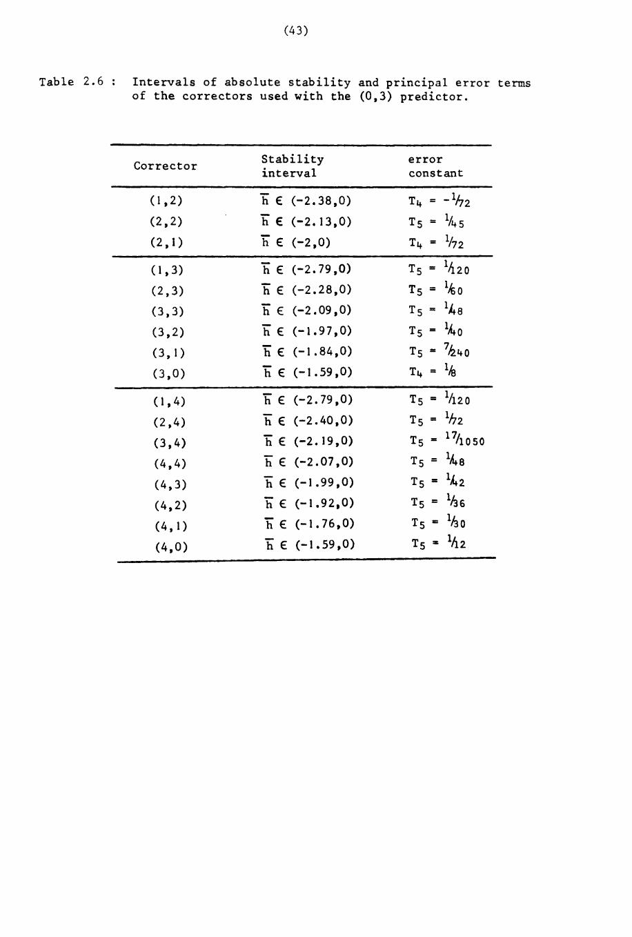
Table 2.6
(43)
Intervals of absolute stability and principal error termsof the correctors used with the (0,3) predictor.
Corrector Stability errorinterval constant
(1 ,2) - (-2.38,0) _11.,2h E T4 =- (-2.13,0) 1/45(2,2) h E TS =- 1172(2,1) h E (-2,0) T4 =
( 1,3) h E (-2.79,0) Ts = 1t1 20
(2,3) hE (-2.28,0) TS = 1ko- (-2.09,0) Ts = 1J.a(3,3) h E
(3,2) h E (-1.97,0) TS = 1ho
(3, 1) h E (-1.84,0) TS = 7&40
(3,0) h E (-1.59,0) T4 = lis
( 1,4) hE (-2.79,0) TS = 11120
(2,4) h E (-2.40,0) Ts = 1h2
(3,4) hE (-2.19,0) TS = 1711 050
(4,4) h E (-2.07,0) TS = 1he
(4,3) hE (-1.99,0) TS = 1h2
(4,2) hE (-1.92,0) Ts = 1136
(4, 1) hE (-1.76,0) TS = 1130
(4,0) h E (-1.59,0) TS = 1112
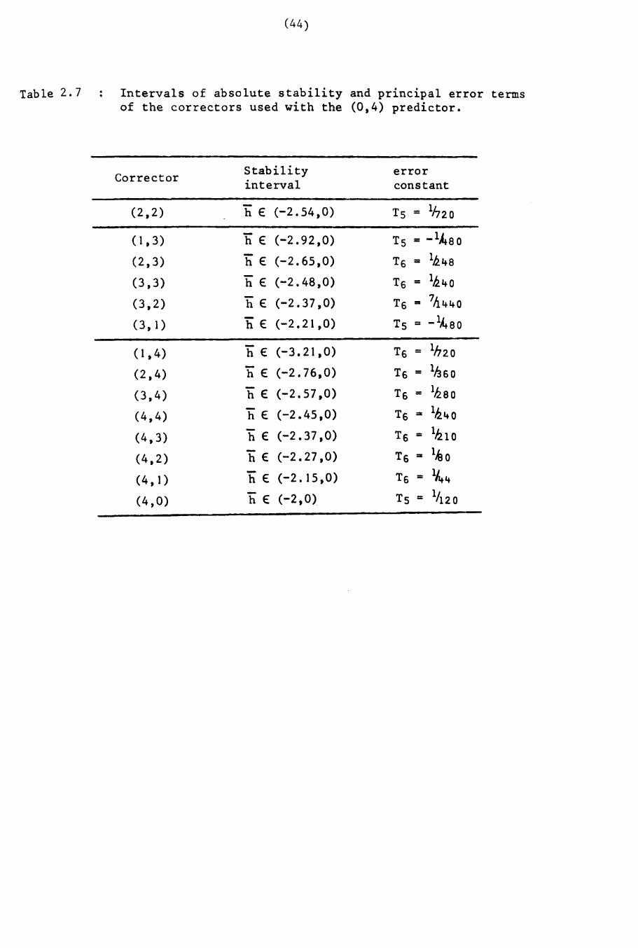
Table 2. 7
(44)
Intervals of absolute stability and principal error termsof the correctors used with the (0,4) predictor.
Corrector Stability errorinterval constant
- (-2.54,0) TS = 1h20(2,2) h E
(1,3) hE (-2.92,0) TS = _l'\a 0
(2,3) hE (-2.65,0) T6 = lk4a
(3,3) h E (-2.48,0) T6 = lk40
(3,2) h E (-2.37,0) T6 = 711440
(3, 1) hE (-2.21,0) TS = _1A.ao
(1,4) h E (-3.21,0) T6 = Ih20
(2,4) hE (-2.76,0) T6 = 11360
(3,4) h E (-2.57,0) T6 = 112 a 0
(4,4) h E (-2.45,0) T6 = 1,240
(4,3) h E (-2.37,0) T6 = 1,210
(4,2) 1i E (-2.27,0) T6 = 1~0
(4, 1) hE (-2.15,0) T6 = 1/4 4
(4,0) h E (-2,0) Ts = l!I20

(45)
2.6 and 2.7, that as (m,k) correctors (m = 1, ... ,k), with in-
creasing individual stability intervals, are used with a g~ven pre-
dictor, the stability intervals in PECE mode decrease. It can also be
deduced that the absolutely stable implicit methods of section 2.2,
have inferior intervals of stability to those methods with finite sta-
bility intervals when used as correctors with any given (O,k) predictor.
Comparisons with the Milne-Simpson and Adams-Bashforth-Moulton com-
binations, show that the results of this section can g~ve much bigger
stability intervals than multi-step methods with the same order of accuracy.
Comparisons with the results of Lawson and Ehle (1970), show that one-step
multiderivative methods can also give comparable accuracy to that of one-
step methods which use high accuracy Newton-Cotes quadrature formulas as
correctors, but can simultaneously give bigger stability intervals. The
use of a combination such as (0,4); (1,5) for instance, would give the
same overall accuracy as the method of Lawson and Ehle (1970), but would
-have a stability interval bigger than h E (-3.21,0), the stability
interval for the (0,4); (1,4) combination which has accuracy one power
fewer than the method of Lawson and Ehle (1970), the method of Lawson and
Ehle (1970) has stability interval h E (-2.07,0).
2.7 Stability Regions
Stability reg~ons, for A complex, associated with the (O,k*); (m,k)
combinations in PECE mode will be plotted from equation (2.33), which is
-TIpECE(r,h) = r - 1 -
k .\' -~
L h p. k• 1 r ,~=
where-h = Ah
+
~s complex.
m . I- k* . ]I (-I)J q . -hJ 1 + ) Pi,k*h~ ,. J,m '=1J =1 -L
The stability region for the (O,k*);(m,k)
combination ~n PECE mode is the reg~on ~n the complex plan determined by
. h stab~l~ty equation (2.34), namelysolv~ng t e -L -L
-( r h) - 0lTpECE ' -
(46)
-for r . Writing h = u + iv (i = +1-1) and r = cos A + i sinA (so
that on the boundary of the region IrJ = 1), equation (2.34) takes the
form
( 2.36) f k* k(u,v) - cos A + i{gk* k(u,v) - sin A} = °,m, ,m,
where A,u,v are real; f,g are real valued functions and clearly change
for each predictor-corrector combination. The stability region for the
(O,k*)
(2.37)
(m,k) combination, is found by solving the non-linear system
f k* k(u,v) - cos A = ° ,,m,
gk* k(u,v) - sin A = ° ,,m,
for each of a serles of values of A in the interval °~ A < 360°.
It was found in section 2.5 that, for k* = 1,2,3,4, the (O,k*); (k*,O)
combination glves the smallest interval of absolute stability when \' < °is real, and that the (O,k*); (m,k) combination gives the biggest stability
interval when m = and k = 4.
here,
The stability regions, for \ complex, of these eight combinations
will now be determined :
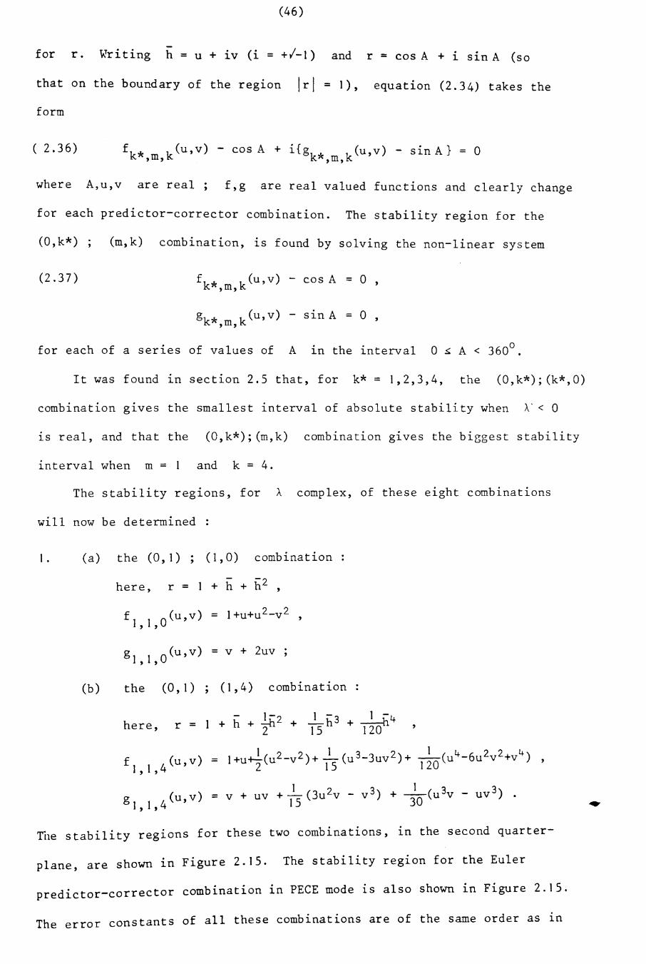
l. (a) the (0,1) ; (1,0) combination
- -2r = 1 + h + h ,
gl,I,O(u,v) = v + 2uv ;
(b ) the (0, 1) ; ( 1, 4) combina t ion
here, r = + h + .!.h2 + _1_ h3 + ~42 15 120
TIle stability regions for these two combinations, in the second quarter-
plane, are shown in Figure 2.15. The stability region for the Euler
d · tor combination in PECE mode is also shown in Figure 2.15.pre lctor-correc
The error constants of all these combinations are of the same order as in
(47)
section 2.5.
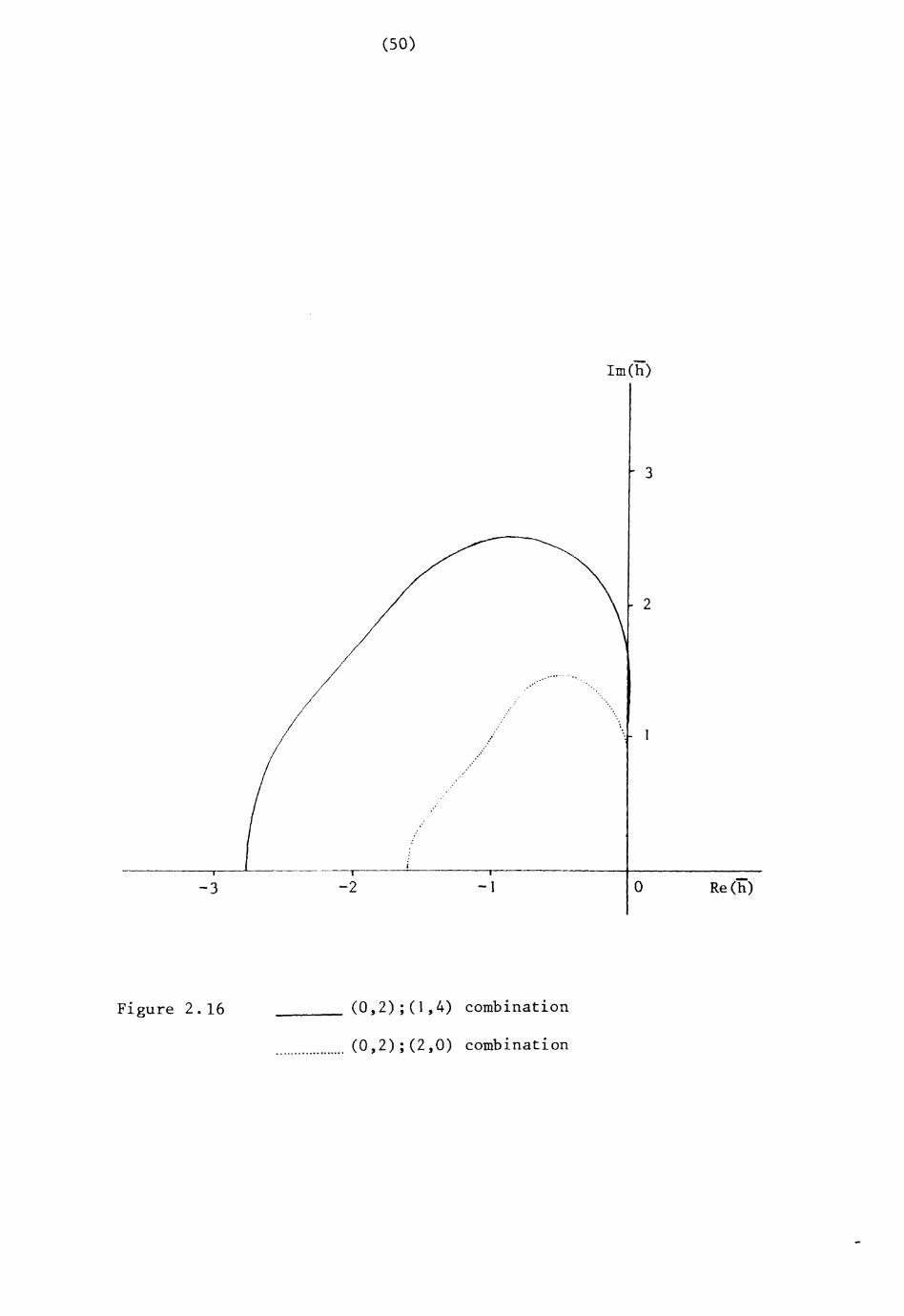
2. (a) the (0,2) ; (2,0) combination
here, r = I + h + l.h2 - ~h42 4
f 2 2 O(u,v) = I + u + l(u2, , 2
8 2 2 O(u,v) = v + uv - u 3v + uv 3, ,
(b) the (0,2); (1,4) combination:
here, r = + h + l.h2 + .!..h3 + _I-h42 6 120
The stability regions for these two combinations are shown in Figure 2.16.
here, r =
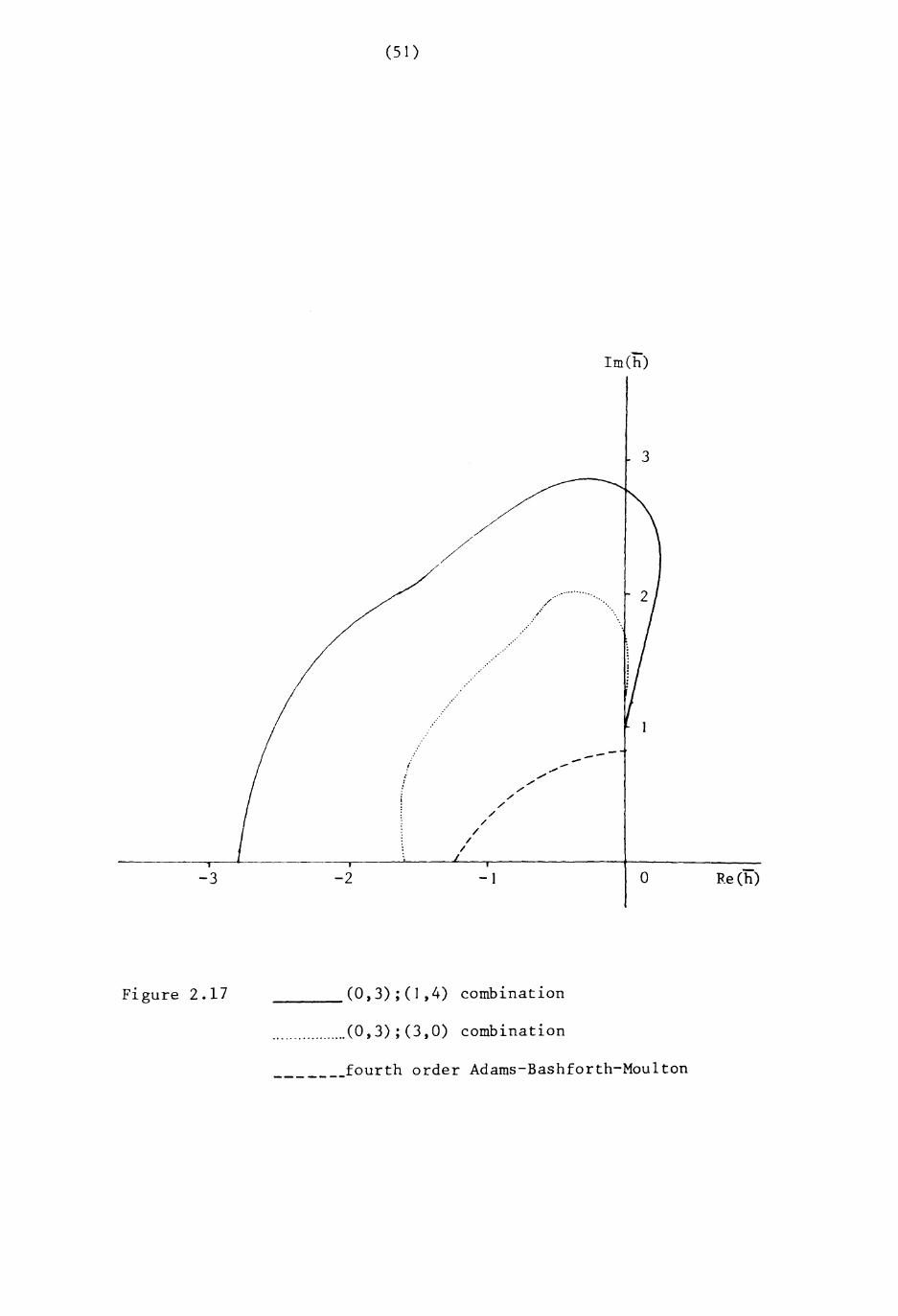
(a) the (0,3)3. (3,0) combination:
+ h + ~2 + J..h3 + _l h4 + _1_ h62 6 12 36
f 3,3,0(u,v) = 1 + u + ~(u2-v2) + ~(u3-3uv2) + /2 (u 4-6u2v2+v4 )
(b) the (0,3) (1,4) combination:
,here, r = - 1-2 1-3 1-+ h + 2"h + 6h + 24 h4
f3
1 4(u,v) = l+u+ l(u2-v 2) + 1.(u 3-3uv2) + _1_ (u 4-6u2v2+v4 ), , 2 6 24
g (u v) - v + uv + 61
(3u 2v - v 3) + 61
(u 3v - uv 3) .3,1,4 ' -
The stability reg10ns for these two combinations are shown in Figure 2.17.
The stability region for the fourth order Adams-Bashforth-Moulton com-
bination in PECE mode, which has the same order error constant as the
(0,3); (1,4) combination in section 2.5, is also shown in Figure 2.17.
here,
(48)
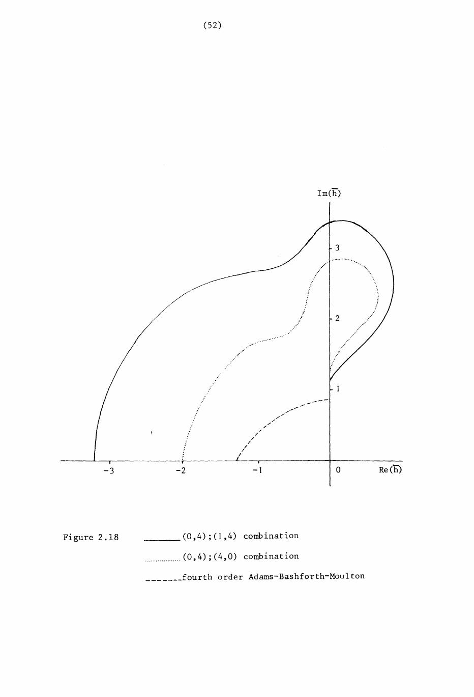
4. (a) the (0,4) ~ (4,0) combination:
r = 1 + h + -}h2 + 61h3 + _1_h4 __1_h6 1-24 72 - 576h 8
f 4,4,0(u,v) = 1 + u + ~(u2-v2) + ~(u3-3uv2) + ~4 (u4-6u2v2+v4)
(b) the (0,4); (1,4) combination:
here,
f 4,1,4(u,v)
The stability regions for these two combinations are shown in
Figure 2.18. The stability region of the fourth order Adams-
Bashforth-Moulton combination, which has the same order error
constant in PECE mode as the (0,4); (4,0) combination, is
also shown in Figure 2.18.
It is noted that the (0,3);(1,4) and (0,4); (1,4) combinations have the
same stability regions as the fourth and fifth order Taylor series methods,
respectively. The axes of all four figures are drawn to the same scale.
The stability regions are, of course, applicable to the system of linear
differential equations of the form
(2.38) y' (x ) = Ay(x) 1.(0) = l{)
(49)
Im(h)
3
2
-------. ......- ....,/ ....,/ "
/ "/ "
/ '// - _.~ \.\ .
/ / \ -.f :/ \ '\
I ./ \I .: \I \ \I \ i, I :I I :
: \!II
-3 -2 -1 o Re(h)
Figure 2.15 ________ (0,1);(1,4) combination
..................... (0,1) ;(1 ,0) combination
_______ (0,1);(1,1) combination (Euler-modified Euler)
(50)
Im(h)
3
-3 -2 -1
2
o Re(h)
Figure 2.16 ______ (0,2) ;(1,4) combination
................... (0,2) ; (2,0) combination
(51)
Im(h)
3
-3 -2
!
.:
......./
,/,/
//
//
//
/
-1
---
° Re(h)
Figure 2.17 _______ (0,3);(1,4) combination
.................. (0,3); (3,0) combination
_______fourth order Adams-Bashforth-Moulton
(52)
Im(h)
....••....
j
2 .....
.......
3
..'./"
..•.
l
....../
---.- ....."' .........
//./
;'./
~
/./
/
/I
-3 -2 -1 o Re(ii)
Figure 2.18 _______ (0,4);(1,4) combination
.................. (0,4); (4,0) combination
_______fourth order Adams-Bashforth-Moulton

where A
(53)
1S square matrix of order N·, the real part of the eigenvalues
A. (J' = 1 2 N), , ...J of A must be non-positive. For non-linear systems
the eigenvalues A.(j = 1,2, ... N) are those of the Jacobian matrixJ
these eigenvalues are calculated at each point x .n
2.8 Numerical examples
The (O,k*);(k*,O). and (0,k*);(l,4) combinations (k = 1,2,3,4)
are tested on two problems, the first a system of the form (2.1) with
-complex eigenvalues, the second a system of the form (2.38) with nega-
tive real eigenvalues but a large stiffness ratio.
Problem 2.1
(Lambert (1973,p.229))
y' =1
y' =2
with initial conditions
Y3 = 40Yl - 40Y2 - 40y3,
TyeO) = (1,0,-1) . The matrix of coefficients
has eigenvalues Al = --2, A2 = -40 + 40i, A3
= -40 - 40i g1v1ng a
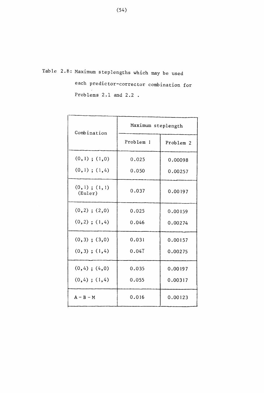
moderate stiffness ratio of 20. The maX1mum steplength for each method
- -is found by drawing the line Im(h) = -Re(h) in Figures 2.15-2.18 and
estimating the point of intersection with the boundary of the stability
region. The maX1mum steplengths for each of the predictor-corrector
combinations follows in an abvious manner and are g1ven 1n Table 2.8,
truncated to three decimal places, together with the maximum steplengths
which may be used with the Euler-modified Euler and Adams-Bashforth-
Moulton combinations.
It was noted by Lambert (1973,p.229), that the theoretical solution
of the problem, g1ven by
1 - 2x 1 - 40x (cos 40x + sin 40x )Yl = - e + - e2 21 - 2x 1 - 40x
(cos 40x + sin 40x)Y2 = - e - e ,2 2
3 - 40x(cos 40x sin 40x )y = -e - ,
(54)
Table 2.8: Maximum steplengths which may be used
each predictor-corrector combination for
Problems 2.1 and 2.2 .
Maximum steplengthCombination
Problem 1 Problem 2
(0, 1) · ( 1,0) 0.025 0.00098,
(0, 1) · (1,4) 0.050 0.00257,
(0,1) ; (1,1)0.037 0.00197(Euler)
(0,2) · (2,0) 0.025 0.00159,
(0,2) · ( 1,4) 0.046 0.00274,
(0,3) · (3,0) 0.031 0.00157,
(0,3) · ( 1,4) 0.047 0.00275,
(0,4) · (4,0) 0.035 0.00197,
(0,4) · ( 1,4) 0.055 0.00317,
A-B-M 0.016 0.00123
(55 )
behaves as ] -2x ] -2x Ty = (~ .~ ,0) for x > 0.] (approximately). The
solution vector was therefore computed only for x ~n the interval
o ~ x ~ 0.09 us~ng the step lengths h = 0.01, 0.015, 0.03.
The numerical results obtained were in keeping with the theory, and
are given for x = 0.09 in Table 2.9. The results for the (0,1);(1,0),
(0,2);(1.2) and (0,3);(3,0) combinations, for which h = 0.03 exceeds
the maximum steplength, display evidence of instability. For all other
combinations, using all three values of h, the error was found to
decay with increasing x.
Problem 2.2
This problem arises ~n reactor
Yi = 0.01 - (0.01 + Yl + Y2)(Y~ + 1001Yl+ 1001) ,
2Y2)(1 + Y2) ,y; = 0.01 - (0.01 + Y
I+
with initial conditions yeO) = (O,O)T.
kinetics and has been discussed by Liniger and Willoughby (1967), Lambert
(1973) and Cash (1980). The Jacobian matrix allay has eigenvalues
;012 and -0.01 at x = 0; it thus has an initial stiffness ratio
~ 105 and may be classed initially as being very stiff. The maximum
steplengths which may be used with the multiderivative predictor-corrector
combinations are found by dividing the value of Re(h), where the curves
bounding the stability regions in Figures 2.15-2.18 cut the real axis, by
-1012. These maximum values, truncated to five decimal places, are given
~n Table 2.8.
One of the maln difficulties in the application of multiderivative
methods to systems of non-linear equations, is in the calculation of the
higher order derivatives. These were easily obtained for the ~resent
problem and were evaluated at each step of the following computations.
The theoretical solution of the problem ~s not known and, following Cash
(1980), was found approximately using the fourth order Runge-Kutta process.
The numerical experiments of Cash (1980,p.245) were repeated using
(56)
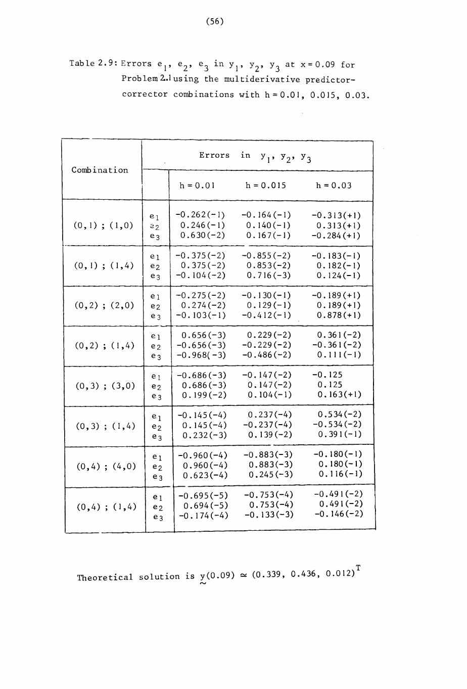
Table 2.9: Errors e 1, e 2, e 3 in Yl' Y2
, Y3
at x=0.09 for
Problem 2.1 using the multiderivative predictor
corrector combinations with h=O.O], 0.0]5, 0.03.
Errors ~n Y1, Y2 , Y3Combination
h=O.OI h = 0.015 h =0.03
el -0.262 (-1) -0. 164 (- I) -0.313(+1)(0,1); (1,0) 22 0.246(-1) O. 140 (-I) 0.313(+1)
e3 o.630 (- 2) 0.167(-1) -0.284(+1)-
el -0.375(-2) -0.855(-2) -0.183(-1)(0,1) ; (],4) e2 0.375(-2) 0.853(-2) 0.182(-1)
e3 -0. 104 (-2) 0.716(-3) O. 124 (-1)
el -0.275(-2) -0. 130 (-1) -0. 189 (+ 1)(0,2) ; (2,0) e2 0.274(-2) 0.129(-1) O. 189 (+ 1)
e3 -0.103(-1) -0.412(-1) 0.878(+1)
el 0.656(-3) 0.229(-2) 0.361 (-2)(0,2) ; (1,4) e2 -0.656(-3) -0.229(-2) -0.361 (-2)
e3 -0. 968( -3) -0.486(-2) 0.111(-1)
el -0.686(-3) -0.147(-2) -0. 125(0,3) ; (3,0) e2 0.686(-3) 0.147(-2) O. 125
e3 0.199(-2) 0.104(-1) 0.163(+1)
el -0. 145 (-4) 0.237(-4) 0.534 (-2)
(0,3) . (1,4) e2 0.145(-4) -0.237(-4) -0.534 (-2),e3 0.232(-3) 0.139(-2) 0.391 (-1)
el -0.960(-4) -0.883(-3) -0. 180 (- I)
(0,4); (4,0) e2 0.960(-4) 0.883(-3) O. 180 (-1)
e3 0.623(-4) 0.245(-3) 0.116(-1)
-el -0.695(-5) -0.753(-4) -0.491(-2)
(0,4); (1,4) e2 0.694(-5) 0.753(-4) 0.491(-2)
e3 -0. 174 (-4) -0.133(-3) -0.146(-2)
TTheoretical solution ~s y(0.09) ~ (0.339, 0.436, 0.012)
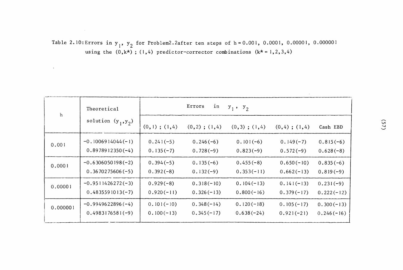
Table 2.10:Errors in Yl' Y2
for Problem2.2after ten steps of h=O.OOl, 0.0001,0.00001,0.000001
using the (O,k*) ; (1,4) predictor-corrector combinations (k* = 1,2,3,4)
Errors.
Theoretical 1n Y1 ' Y2h
solution (y l' y 2)(0, I) ; (1,4) (0,2); (1,4) (0,3); (1,4) (0,4) ; (1,4) Cash EBD
0.001-0.1006914044(-1) 0.241(-5) 0.246(-6) O. 10 1(-6) 0.149(-7) 0.815(-6)
0.8978912350(-4) 0.135(-7) 0.728(-9) 0.823(-9) 0.572(-9) 0.628(-8)
0.0001-0.6306050198(-2) 0.394(-5) 0.135(-6) 0.455(-8) 0.650(-10) 0.835(-6)
0.3670275606(-5) 0.392 (-8) 0.132(-9) 0.353 (-11) 0.662(-13) 0.819(-9)
0.00001-0.9511426272(-3) 0.929(-8) 0.318(-10) 0.104(-13) 0.141(-13) 0.231(-9)
0.4835591013(-7) 0.920 (-11) 0.326(-13) 0.800(-16) 0.379 (-17) 0.222(-12)
0.000001-0.9949622896(-4) 0.101(-10) 0.348(-14) 0.120(-18) 0.105(-17) 0.300 (-13)
0.4983176581(-9) O. 100 (-13) 0.345 (-17) 0.638(-24) 0.921(-21) 0.246(-16)
""'lJ1'-J<;»
(58)
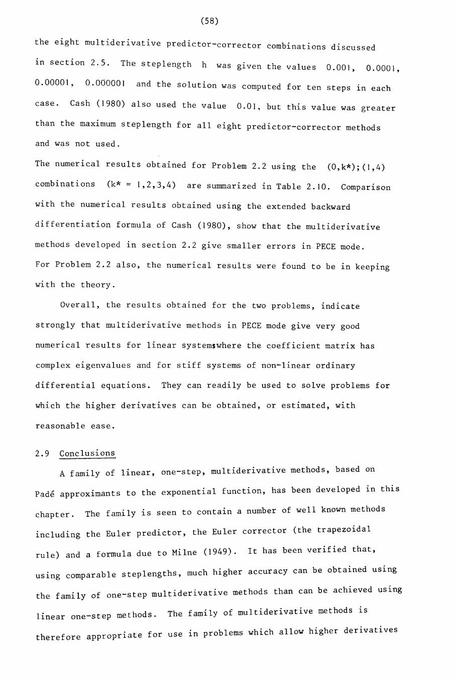
the eight multiderivative predictor-corrector combinations discussed
in section 2.5. The steple th h 0 hng was glven t e values 0.001, 0.0001,
0.00001, 0.000001 and the solution was computed for ten steps in each
case. Cash (1980) also used the value 0 01 b t thO 1 t. ,u 1S va ue was grea er
chapter.
than the maximum steplength for all eight predictor-corrector methods
and was not used.
The numerical results obtained for Problem 2.2 uS1ng the (0,k*);(1,4)
combinations (k* = 1,2,3,4) are summarized in Table 2.10. Comparison
with the numerical results obtained using the extended backward
differentiation formula of Cash (1980), show that the multiderivative
methods developed in section 2.2 give smaller errors in PECE mode.
For Problem 2.2 also, the numerical results were found to be in keeping
with the theory.
Overall, the results obtained for the two problems, indicate
strongly that multiderivative methods in PECE mode give very good
numerical results for linear systemswhere the coefficient matrix has
complex eigenvalues and for stiff systems of non-linear ordinary
differential equations. They can readily be used to solve problems for
which the higher derivatives can be obtained, or estimated, with
reasonable ease.
2.9 Conclusions
A family of linear, one-step, multiderivative methods, based on
o h been developed 1n thisPade approximants to the exponential funct10n, as
The family is seen to contain a number of well known methods
o h E 1 r corrector (the trapezoidalincluding the Euler pred1ctor, t e u e
rule) and a formula due to Milne (1949). It has been verified that,
h h o h accuracy can be obtained usinguS1ng comparable steplengths, muc 19 er
the family of one-step multiderivative methods than can
d The family of multiderivativelinear one-step metho s.
be achieved uS1ng
methods is
use 1n problems which allow higher derivativestherefore appropriate for
(59)
to be found explicitly and which requlre high accuracy. Intervals of
absolute stability have been calculated and it is seen that those
members of the ,family which are fully implicit, in the sense that the
highest derivative must be evaluated at the advanced point, are
absolutely stable.
The family of multiderivative methods has been extrapolated to
achieve higher accuracy and intervals of absolute stability are cal
culated for the extrapolation formulas. It is seen that, whilst
extrapolation increases accuracy, stability intervals are sometimes
shortened as a consequence; the most notable example of this is the
trapezoidal rule.
Finally, the family of one-step multiderivative methods has been
used in appropriate predictor-corrector pairs. Error constants, stability
intervals and stability regions have been calculated for PECE mode. As
with linear multistep (single derivative) methods used in PECE mode, the
stability intervals are seen to be somewhat low. It is clear from Tables
2.4, 2.5, 2.6 and 2.7 however, that it is possible to achieve a bigger
stability interval, with comparable accuracy, uSlng one-step multi
derivative combinations in PECE mode than with some well known multi-step
combinations, notably the Milne-Simpson and Adams~Bashforth-Moulton
methods, or with one-step methods using high accuracy Newton-Cotes
quadrature formulas as correctors.
(60)
CHAPTER 3
SECOND ORDER PARABOLIC EQUATIONS
3.1 Introduction
In recent papers, Lawson and Swayne (1976), Lawson and Morris (1978)
and Gourlay and Morris (1980), attention has been devoted to the develop
ment of Lo-stable methods for the numerical solution of second order
parabolic partial differential equations for which Ao-stable methods
c ,~h as the Crank-Nicolson method, are uns a t i s f ac r r- .... '7 "1...,.._::,l _:TIe
discretization is used with time steps which are too large relative to
the space discretization, see for example, Smith et al (1973) and Wood
and Lewis (1975).
Lawson and Morris (1978) developed a second order LO-stable method
as ar. cytrapolation of a first order backward difference method in one and
two space dimensions. This idea was developed further for one space
variable by Gourlay and Morris (1980) who achieved third and fourth order
accuracy in time by a novel multistage process. The second order method
of Lawson and Morris (1978), was adapted and used in a practical problem
involving a non-linear parabolic equation by Twizell and Smith (1981, 1982).
The extrapolation procedure of Lawson and Horris (1978) involved
computing the solution of the parabolic equation at time t + 2£, ln terms
of the solution at time t, uSlng a first order method with time step £.
second order accuracy was thus achieved. Gourlay and Morris (1980) extended
the principal by computing the solution at time t + 3£, ln terms of the
solution at time t, using a time step £, and thus achieved third order
accuracy in time. These authors then went further, and achieved fourth
order accuracy by computing the solution at time t + 4£ in terms of the
solution at time t.
The multistage methods which evolved in this way involved a "spread"
ln time. In this chapter a family of methods will be developed which
involves a similar "spread" ln space, in that an increased number of points
at each time level are used ln the resulting finite difference schemes.
(61)
This concept of us~ng a greater number of points at each time level was
used by Twizell (1979) for second order hyperbolic equations and by
Khaliq and Twizell (1982) for first order hyperbolic equations; the
concept is discussed for second order parabolic equations in the text
by Mitchell and Griffiths (1980).
The methods developed are applications of the methods for a system
of first order ordinary "differential equations discussed in Chapter 2.
Following Lawson and Morris (1978) and Gourlay and Morris (1980), the
space derivatives will be approximated by the usual second order central
difference replacement. The principal part of the local truncation error
of each finite difference scheme will, therefore, include the same
component proportional to £h2 , where h is the space step, encountered,
though not stated explicitly, in Lawson and Morris (1978) and Gourlay and
Morris (1980). This component notwithstanding, it was shown in Lawson and
Morris (1978) and Gourlay and Morris (1980), that extrapolation in time
leads to a worthwhile improvement in accuracy; this being demonstrated
clearly by numerical experiments reported in those papers.
The family of multiderivative methods on which the finite difference
schemes are based, uses Pade approximants to the matrix exponential function.
Lawson and Morris (1978) used the (1,0) Pade approximant; in this
chapter, four higher order Pade approximants are used to achieve higher
order accuracy in time. The resulting finite difference schemes are im
plicit ~n nature and each requires one quindiagonal or sevendiagonal
solver to determine the solution. This compares well with the multistage
methods in Gourlay and Morris (1980) where, for problems with one space
vari~ble, five applications of a tridiagonal solver are needed to achieve
third order accuracy in time and at least seven applications of a tri
diagonal solver to achieve fourth order accuracy in time.
The methods developed in this Chapter will be tested on the model
problems used in Lawson and Morris (1978) and Gourlay and Morris (1980).
(62)
For one space variable. the second order method will be seen to glve
results comparable overall to the best third order multistage methods
in Gourlay and Morris (1980), and third order methods developed ,to give
results comparable overall to the best fourth order multistage method.
3.2 One-space dimension
Consider the constant coefficient heat equation 1n one space
variable
(3. I) dUdt = o < x < X , t > 0
with initial conditions
(3.2) u(x,O) = g(x) o .::;; x s X
and boundary conditions
(3.3) u(O,t) = u(X,t) = 0 t > 0
In (3.2), g(x) 1S a glven continuous function of x; it 1S not
specified that g(O) = 0 or g(X) = 0, so that discontinuities between
initial conditions and boundary conditions may occur.
The interval 0.::;; x .::;; X is divided into N+I subintervals each of
width h so that (N+I)h = X, and the time variable t is discretized
in steps of length £. The open reg10n R = [0 < x < XJ x [t > OJ and
its boundary aR have thus been covered by a rectangular mesh, the mesh
points having co-ordinates (mh,n£) with m = O,I, ... ,N+I and
n = 0,1,2, ... The notationn
u = u(mh,n£)m
will be used to denote the
solution of (3.1) while un will be used to denote the theoreticalm
solution of an approximating finite difference scheme.
The space derivative in (3.1) is now replaced by
(3.4)= {u(x-h,t)-2u(x,t)+u(x+h,t)}/h2+O(h2 )
and (3.1) with (3.4) is applied to all N interior mesh points at time
t = n£ (n = 0,1, ... ). This produces a system of ordinary differential
equations of the form
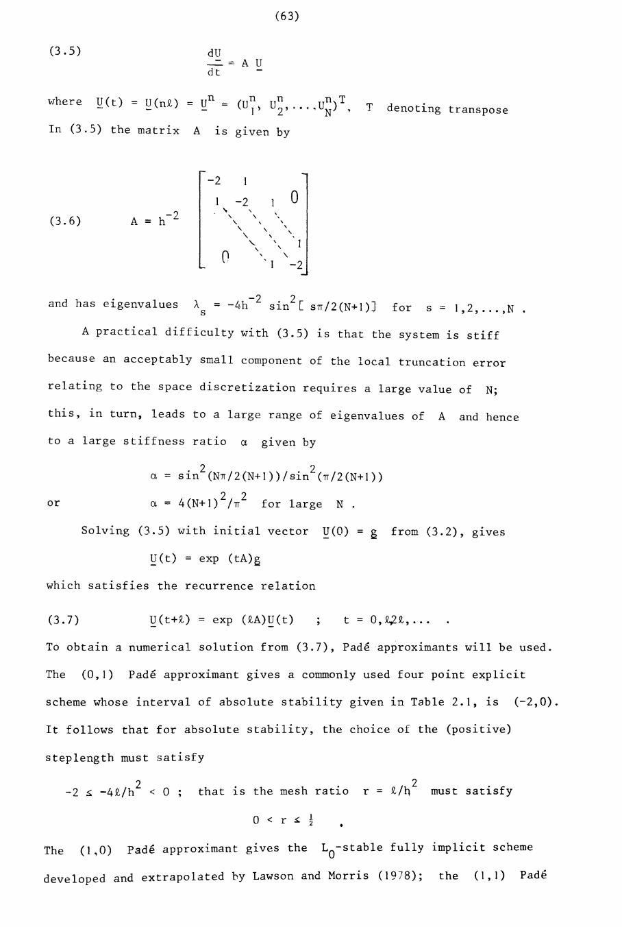
(3.5) dU
dt= A U
(63)
where U(t) = U(n£)- - T denoting transpose
In (3.5) the matrix A 1S given by
-2
-2 o-2 ~ , ,
(3.6) A, , ,= h , , ,, ,, ,, ,, ,, ,
0 , ,, I -2
and has eigenvalues -2 2~ = -4h sin [ sn/2(N+I)Js for s = 1,2, ... ,N
A practical difficulty with (3.5) is that the system is stiff
because an acceptably small component of the local truncation error
relating to the space discretization requires a large value of N·,
this, in turn, leads to a large range of eigenvalues of A and hence
to a large stiffness ratio a given by
or
a =
a =
sin2(Nn/2(N+I»/sin2(n/2(N+I»
4(N+I)2/n2 for large N.
Solving (3.5) with initial vector ~(O) = g from (3.2), gives
~(t) = exp (tA)g
which satisfies the recurrence relation
(3.7) ~(t+£) = exp (£A)~(t) t = o,~£, ...
To obtain a numerical solution from (3.7), Pade approximants will be used.
The (0,1) Pade approximant gives a commonly used four point explicit
scheme whose interval of absolute stability given in Table 2.1, is (-2,0).
It follows that for absolute stability, the choice of the (positive)
step length must satisfy
2-2 ~ -4£/h < ° ; that 1S the mesh ratio r = must satisfy
° < r ~ ! •
The (1,0) Pade approximant gives the Lo-stable fully implicit scheme
developed and extrapolated by Lawson and Morris (1978); the (1,1) Pad€
(64 )
approximant g1VeS the A -stable era k~' 1 h~ ° n -~1CO son met od which was alsc
analysed in Lawson and Morris (1978).
Employing the (m k) Pade~ a .~ pprox1mants~ for m < k, to the
exponential function in (3.7), will yield explicit or semi-explicit
methods, whose intervals of stability may be calculated from Table 2.1.
In the following sections four higher order Pade approximants with the
degree of the numerator "less than or equal to the degree of denominator,
will be used in (3.7) and the resulting algorithms analysed.
3.3 A second order method and its extrapolation
Using the (2,0) Pade approximant to exp(£A) 1n (3.7) g1ves
(3.8)
suggesting the fully implicit scheme
(3.9)
Following Gourlay and Morris (1980), a stability analysis verifies that
(3.9) is Lo-stable, and using Taylor's theorem it is found that the
principal part of the local truncation error at the mesh point (mh,n£)
for m = 2, ... ,N-l and n = 0,1,2, ... 1S
(3.10) ,
though this accuracy 1S not attained at points adjacent to the boundaries.
This phenomenon is seen to be present in all the subdiagonal Pade approxi-
mants for time dependent problems except the (1,0) Pade approximant. In
a paper on hyperbolic equations, Oliger (1974,p.20) showed that using
lower approximants near the boundaries, does not affect the stability or
convergence properties of the scheme as a whole, and the numerical evidence
to be reported in section 3.6 suggests that this is true for second order
parabolic equations also.
In (3.10) the component 1S due to the space dis-
cretization and the use of (3.4) 1n (3. I); this term will appear in the
local truncation error of every finite difference scheme arising from the
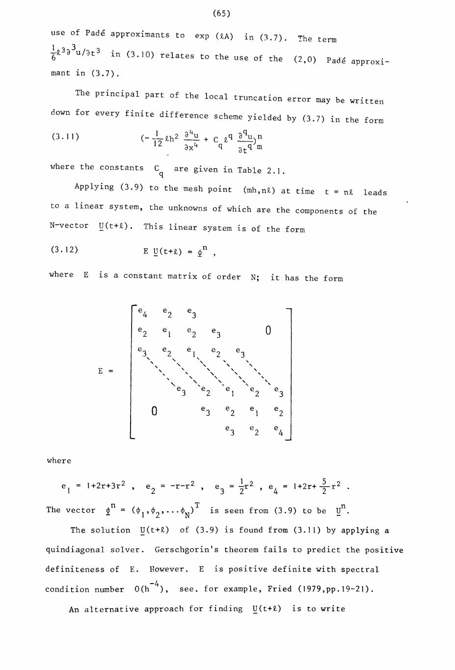
(65)
use of Pade approximants to exp (£A) ln (3.7). !he term
~~3d3u/dt3 in (3.]0) relates to the use of the (2,0) Pade approxi
mant in (3.7).
The principal part of the local truncation error may be written
down for every finite difference scheme yielded by (3.7) in the form
(3.11)
where the constants C are given in Table 2.1.q
Applying (3.9) to the mesh point (mh,n£) at time t = n£ leads
to a linear system, the unknowns of which are the components of the
N-vector U(t+£). This linear system is of the form
(3 • 12)
where E
E ~(t+£) = ~n ,
1S a constant matrix of order N·, it has the form
where
e4 e2 e
3
e2 e
1 e2 e
3 ae
3 e2 e1 e
2 e3
'- '-, , ,,,
" '-, ,
'- '- , '- ,E = ,'- " '- '-,
'- '- , ,," '- , ,
-, , '-,e
1e
2e
3e
3e
2
0 e3
e2
e1
e2
e3
e2
e4
e = 1+2r+3r21
e = -r-r 2 ,2
e = 1 2 = 1+2r+ 52 r 2 •3 i r , e4
The solution
The vector 2n = T(¢I'¢2' ... ¢N) 1S
U(t+£) of (3.9)
) b Un .seen from (3.9 to e
is found from (3.11) by applying a
quindiagonal solver. Gerschgorin's theorem fails to predict the positive
definiteness of E. However. E is positive definite with spectral
condition number see, for example, Fried (1979,pp.19-21).
An alternative approach for finding ~(t+£) is to write
(66)
E = I-oA + ~o2A2 "t 1h 2h. 1n 1 s comp ex factor form. namely
E = ~ {(I + i)I -Q,A} {(I - i)I -Q,A)} , 1 = + ';-1
This suggests the complex splitting
(3. 13)
{( .) *1 - 1 I - Q,A} ~ = ~(t)
~{(1 + i) - Q,A} ~(t+Q,) = U*
The solution ~(t+Q,) 1S obtained from (3.13) by the application of two
tridiagonal solvers using complex arithmetic. This is less efficient,
in that it uses more CPU time, than using one quindiagonal solver with
real arithmetic and (3.11) is therefore to be preferred to (3.13).
It has been noted already that (3.9) is Lo-stable; it may
therefore be extrapolated to improve the accuracy in time.
First of all, ~(1) = g(l) (t+2Q,) 1S computed by applying (3.7)
over two single time steps with exp(Q,A) replaced by its (2,0) Pade
approximant; secondly, g(2) = g(2) (t+2Q,) is computed by applying
(3.7) over a double time step. In general, the extrapolated value
U(E)= g(E) (t+2Q,) 1S determined from the formula
(3, 14)
where
(3. 15) a = 2m+k / (2m+k_l) ,
4so that for the (2,0) Pade approximant, a = 3
The principal part of the local truncation error of the extrapolated form
of each finite difference method arising from using the (m,k) Pade
m = 2,.",N-l(3. 16)
, t to exp (OA) ln (3 7) will be of the formapprox1man x. • ,
(__1_Q,h2 a4u + E Q,P aPu)n12 ax 4 p atP m
where p = m+k+2. The constants
contained in Table 2.3; for the
E (Twizell and Khaliq (1981)), arep
1(2,0) Pade approximant, E4= - 3'
. symbol of the extrapolated form of the methodThe amplificatl0n
arising from using the (m,k) Pade approximant in (3.7), 1S
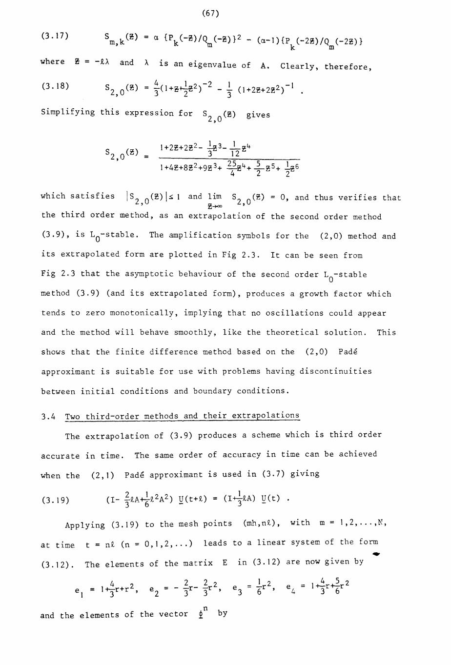
(3. 17)
(67)
S k(n) = a {p (-n)/Q (-n)}2m, k m (a-l){P (-2n)/Q (-2n)}
k m
where n = -tA and .1S an eigenvalue of A. Clearly~ therefore,
(3 . 18)
Simplifying this expression for S2 O(n) g1ves,
which satisfies \S2,0(n)!.s; 1 and lim S2,0(~) = 0, and thus verifies that~~
the third order method, as an extrapolation of the second order method
(3.9), is Lo-stable. The amplification symbols for the (2,0) method and
its extrapolated form are plotted in Fig 2.3. It can be seen from
Fig 2.3 that the aSYmptotic behaviour of the second order Lo-stable
method (3.9) (and its extrapolated form), produces a growth factor which
tends to zero monotonically, implying that no oscillations could appear
and the method will behave smoothly, like the theoretical solution. This
shows that the finite difference method based on the (2,0) Pade
approximant is suitable for use with problems having discontinuities
between initial conditions and boundary conditions.
3.4 Two third-order methods and their extrapolations
The extrapolation of (3.9) produces a scheme which 1S third order
accurate in time. The same order of accuracy in time can be achieved
when the (2,1) Pade approximant 1S used in (3.7) giving
(3.19)
Applying (3.19) to the mesh points (mh,n£), with m = 1,2, ... ,N,
at time t = n£ (n = 0,1,2, ... ) leads to a linear system of the form~
(3.12). The elements of the matrix E 1n (3.12) are now g1ven by
1 t ~ r+r 2, 222 1 2 45 2e3
= (;r , e4
= 1+-r+-re1 = e = - -r- -r 3 62 33'
!fin byand the elements of the vector ~
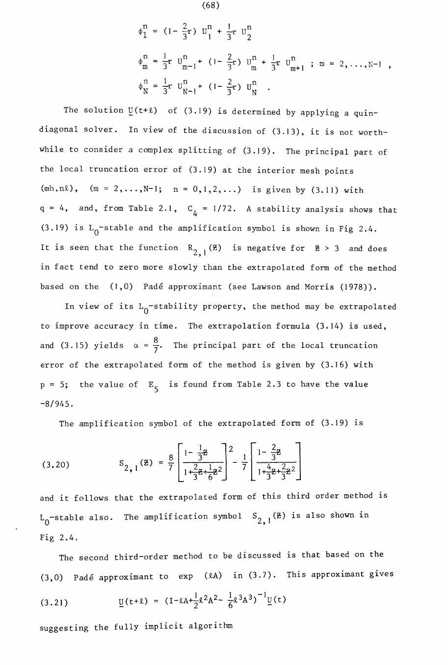
(68)
¢~')
Un ] Un= (I - ....r) + -r3 1 3 2
¢n I Un 2 Un J Un= -r + (1- -r) + -r m = 2, ... ,N-Im 3 m--) 3 m 3 m- l ,
¢n 1 Un + 2 Un= -r (1- Ir)N 3 N-l N
The solution ~(t+~) of (3.19) is determined by applying a qu~n-
diagonal solver. In view of the discussion of (3.13), it is not worth-
while to consider a complex splitting of (3.19). The principal part of
the local truncation error of (3.19) at the interior mesh points
(mh,n~), (m = 2, ... ,N-l; n = 0,1,2, ... ) is given by (3.11) with
q = 4, and, from Table 2.1, C4
= 1/72. A stability analysis shows that
(3.19) is Lo-stable and the amplification symbol ~s shown in Fig 2.4.
It is seen that the function R2 I (~) ~s negative for ~ > 3 and does,~n fact tend to zero more slowly than the extrapolated form of the method
based on the (1,0) Pade approximant (see Lawson and Morris (1978)).
In view of its Lo-stability property, the method may be extrapolated
to ~mprove accuracy in time. The extrapolation formula (3.14) is used,
and (3. IS) yields8
a = 7' The principal part of the local truncation
error of the extrapolated form of the method is given by (3.16) with
p = 5;
-8/945.
the value of E5
is found from Table 2.3 to have the value
The amplification symbol of the extrapolated form of (3.19) ~s
(3.20)
and it follows that the extrapolated form of this third order method ~s
Lo-stable also.
Fig 2.4.
The amplification symbol s (~) is also shown in2, I
The second third-order method to be discussed ~s that based on the
(3,0) Pade approximant to exp (~A) in (3.7). This approximant g~ves
0.21)
suggesting the fully implicit algorithm
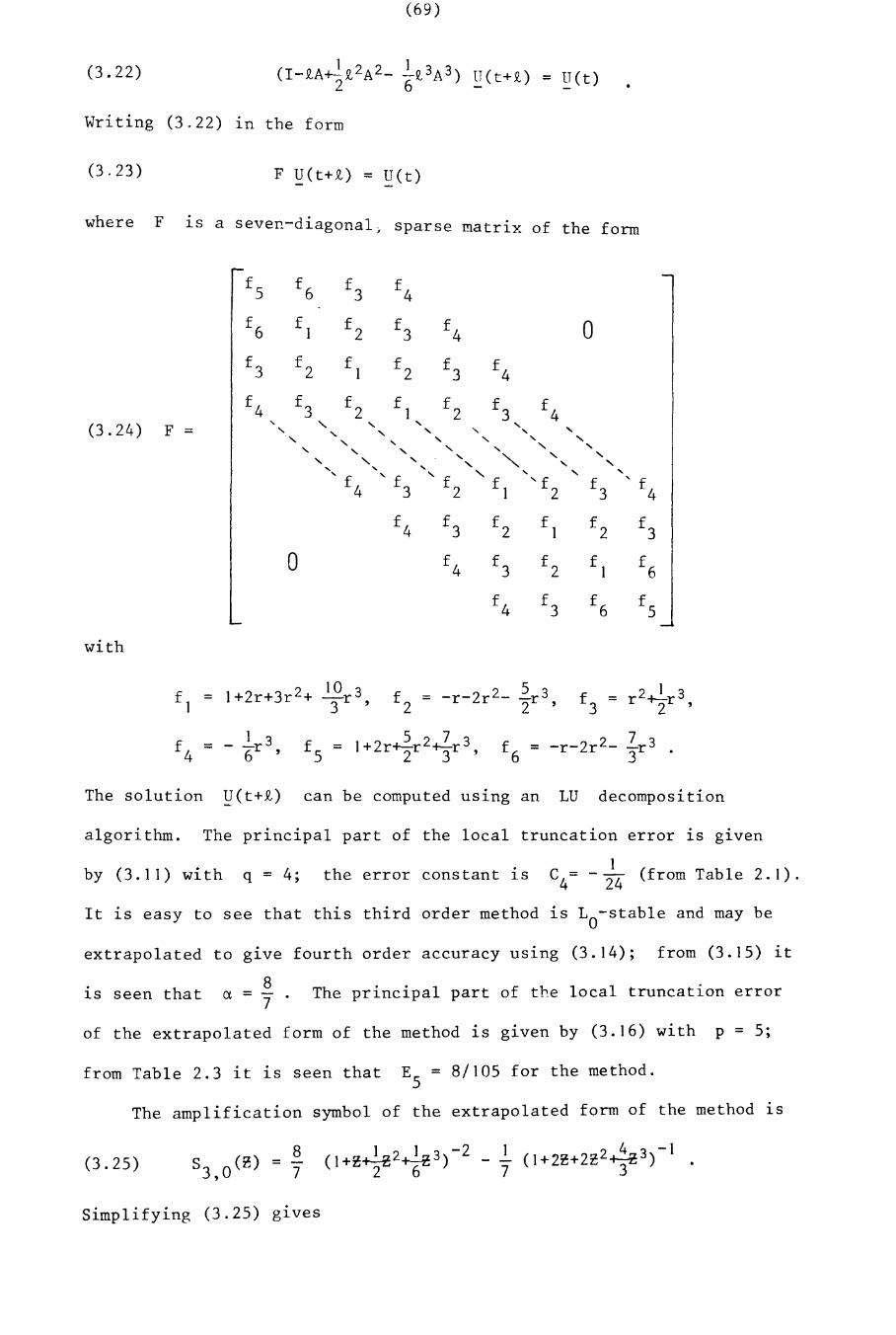
(69)
(3.22) (I-g,A~g,2A2- }_£3A3) !:!(t+£) = U(t)2 6
Writing (3.22) 1.n the form
(3.23 ) F !.!(t+£) = !l(t )
where F 1.S a seven-diagonal, sparse matrix of the form
f5
f6 f
3f
4
f6
f1 f
2f
3f
4 0f
3f
2 f1
f2
f3
f4
f4
f3
f2
f1
f2
f3
f4
(3.24 ).... ...... "
,"F = "- -, " " -, , "" "
, "- ",
"" " " " "-, "
" -, " " -, " "" "- ""- .... "" f ' f " f<, " "
,f
1'f f
3.... f
4 3 2 2 4
f4
f3
f2
f1
f2
f3
0 f4
f3
f2
f1
f6
f4
f3
f6
f5
with
f = - l..r 34 6'
The solution ~(t+g,) can be computed using an LV decomposition
algorithm. The principal part of the local truncation error is given
by (3.11) with q = 4; the error constant is1
C4= - 24 (fr om Tab I e 2. I ) .
It is easy to see that this third order method is La-stable and may be
extrapolated to give fourth order accuracy using (3.14); from (3.15) it
1.S seen that8
Ct = -7
The principal part of the local truncation error
of the extrapolated form of the method is given by (3.16) with p = 5;
from Table 2.3 it is seen that E = 8/105 for the method.5
The amplification sYmbol of the extrapolated form of the method 1.S
(3.25 ) ( ~ ) 8 (1+~~212~61 3)-2S3, a ~ = 7
Simplifying (3.25) g1.ves
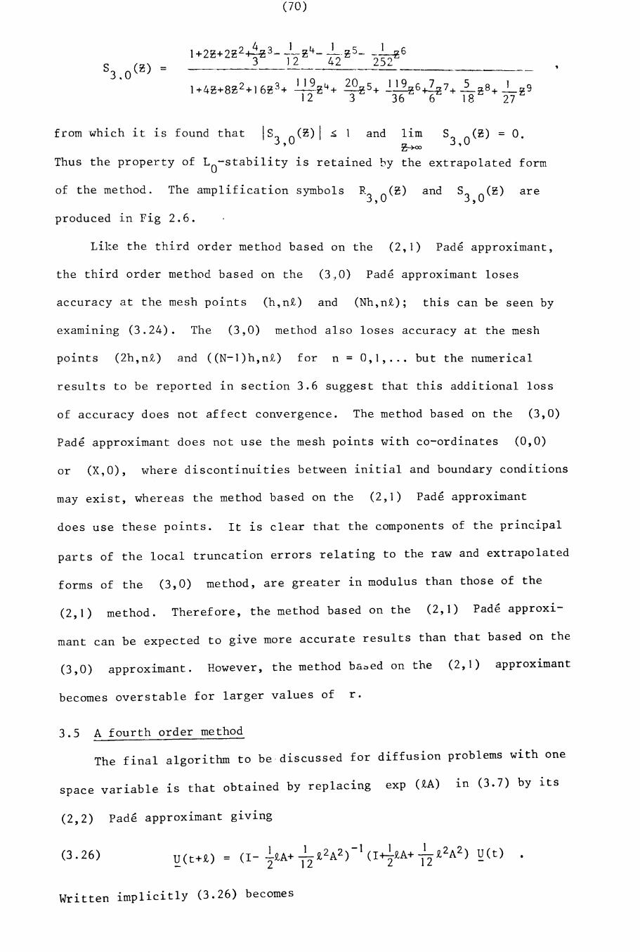
(70)
of the method.
from 'which it is found that IS3,0(~) I s 1 and ~ S3,0(~) = 0.
Thus the property of Lo-stability is retained by the extrapolated form
The amplification sYmbols R3,0(~) and S3,0(~) are
produced in Fig 2.6.
Like the third order method based on the (2,1) Pade approximant,
t h e third order method based on the (3 0) Pade~ appro ~ a t I1 xLm noses
accuracy at the mesh points (h,n£) and (Nh,n£); this can be seen by
examining (3.24). The (3,0) method also loses accuracy at the mesh
points (2h,n£) and ((N-l)h,n£) for n = 0,1, ... but the numerical
results to be reported in section 3.6 suggest that this additional loss
of accuracy does not affect convergence. The method based on the (3,0)
Pade approximant does not use the mesh points with co-ordinates (0,0)
or (X,O), where discontinuities between initial and boundary conditions
may exist, whereas the method based on the (2,1) Pade approximant
does use these points. It is clear that the components of the principal
parts of the local truncation errors relating to the raw and extrapolated
forms of the (3,0) method, are greater in modulus than those of the
(2,1) method. Therefore, the method based on the (2,1) Pade approxi-
mant can be expected to give more accurate results than that based on the
(3,0) approximant. However, the method ba~ed on the (2,1) approximant
becomes overstable for larger values of r.
3.5 A fourth order method
The final algorithm to be discussed for diffusion problems with one
space variable is that obtained by replacing exp (£A) in (3.7) by its
(2,2)
(3.26 )
. .Pade approximant g~v~ng
Written implicitly (3.26) becomes
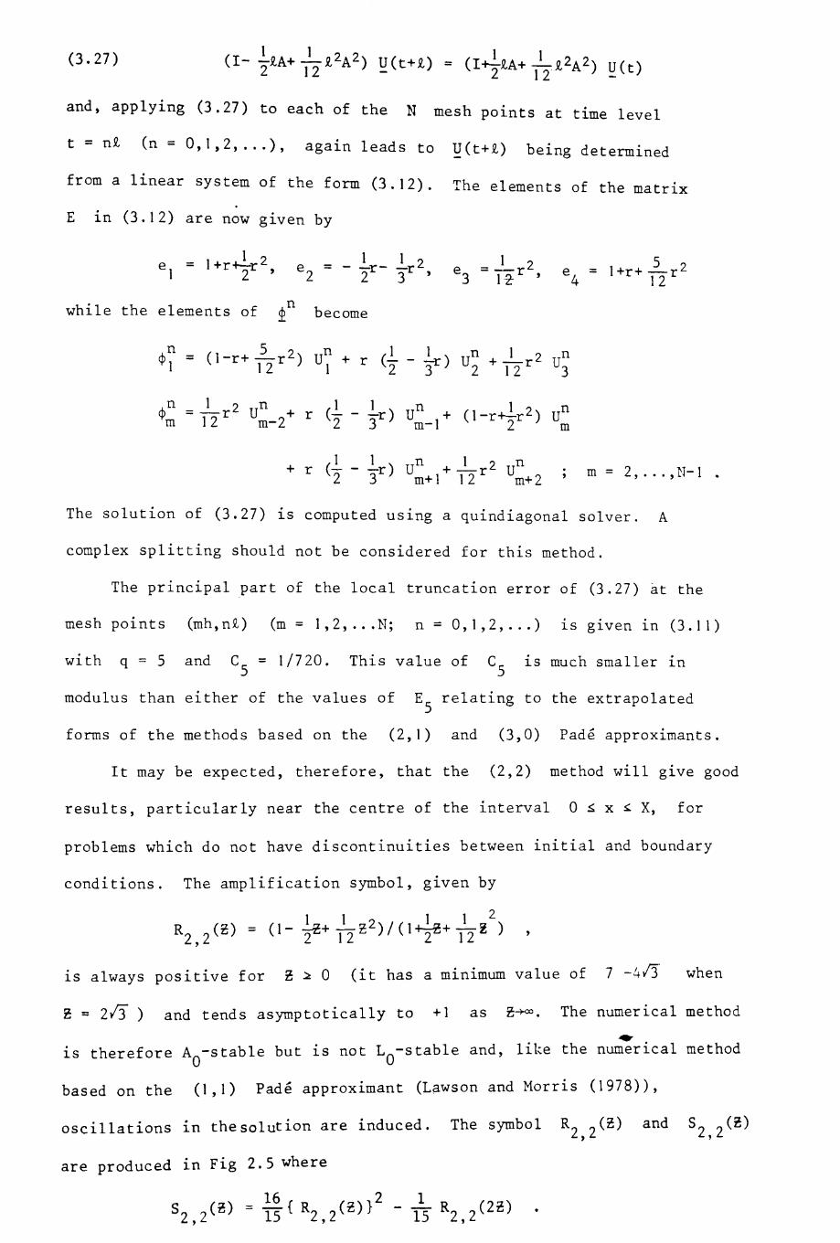
(3.27)
and, applying (3.27) to each of the N mesh points at time level
t = n£ (n = 0,1,2, ... ), again leads to ~(t+£) being determined
from a linear system of the form (3.12). The elements of the matrix
E in (3.12) are now glven by
e = l+r~... 21 2.L ,
while the elements of IfIn b:r ecome
A-.n = _1_r 2 n ( 1 1 u" + 1 2 u""rn 12 Um- 2+ r 2" - 3'r) m--I (l-r+zr) m
m = 2, ... , N-l
The solution of (3.27) is computed uSlng a quindiagonal solver. A
complex splitting should not be considered for this method.
The principal part of the local truncation error of (3.27) at the
mesh points (mh,n£) (m = 1,2, ... N; n = 0,1,2, ... ) lS given in (3.11)
wi th q = 5 and C = 1/720.5
This value of lS much smaller in
modulus than either of the values of E5
relating to the extrapolated
forms of the methods based on the (2,1) and (3,0) Pade approximants.
It may be expected, therefore, that the (2,2) method will give good
results, particularly near the centre of the interval ° ~ x ~ X, for
problems which do not have discontinuities between initial and boundary
conditions. The amplification symbol, given by
is always positive for ~ ~ ° (it has a minimum value of 7 -4/3 when
~ = 213) and tends asymptotically to +1 as ~~. The numerical method...is therefore Ao-stable but is not Lo-stable and, like the numerical method
based on the (1,1) Pade approximant (Lawson and Morris (1978)),
oscillations in thesolution are induced. The symbol R2,2(~) and S2,2(~)
are produced in Fig 2.5 where
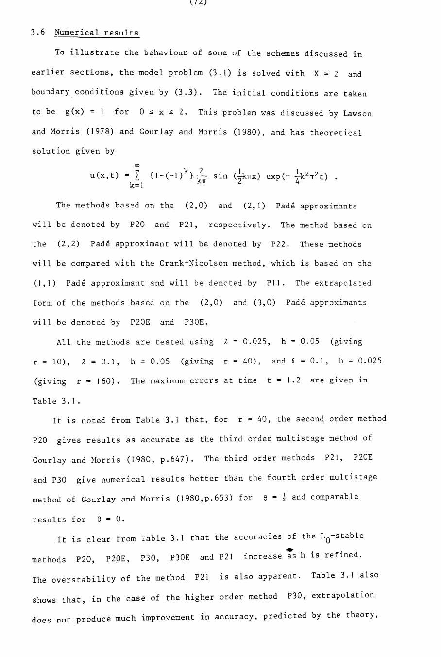
l..IL)
3.6 Numerical results
To illustrate the behaviour of some of the schemes discussed in
earlier sections, the model problem (3.1) is solved with X = 2 and
boundary conditions given by (3.3). The initial conditions are taken
to be g(x) = 1 for ° ~ x ~ 2. This problem was discussed by Lawson
and Morris (1978) and Gourlay and Morris (1980), and has theoretical
solution given by
00
u(x~t) = Lk=l
{1- (- l ) k } _2 (1 1 2 2k~ Sln Zk~x) exp(- 4k ~ t)
The methods based on the (2,0) and (2,1) Pade approximants
will be denoted by P20 and P21, respectively. The method based on
the (2,2) Pade approximant will be denoted by P22. These methods
will be compared with the Crank-Nicolson method, which lS based on the
(1,1) Pade approximant and will be denoted by Pl1. The extrapolated
form of the methods based on the (2,0) and (3,0) Pade approximants
will be denoted by P20E and P30E.
All the methods are tested using £ = 0.025, h = 0.05 (giving
r = 10), £ = 0.1, h = 0.05 (giving r = 40), and £ = 0.1, h = 0.025
(giving r = 160). The maximum errors at time t = 1.2. .
are glven In
Table 3. 1 .
It is noted from Table 3.1 that, for r = 40, the second order method
P20 gives results as accurate as the third order multistage method of
Gourlay and Morris (1980, p.647). The third order methods P21, P20E
and P30 give numerical results better than the fourth order multistage
method of Gourlay and Morris (1980,p.653) for e = ~ and comparable
results for e = 0.
It is clear from Table 3.1 that the accuraCles of the Lo-stable..methods P20, P20E, P30, P30E and P21 increase as h is refined.
The overstability of the method P21 is also apparent. Table 3.1 also
shows that, in the case of the higher order method P30, extrapolation
does not produce much improvement in accuracy, predicted by the theory,
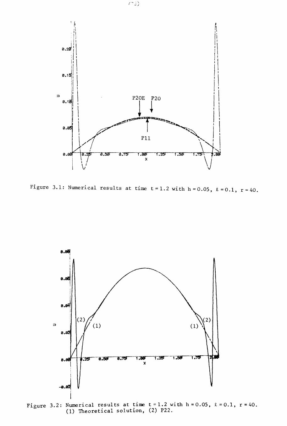
r r : "\-;
Figure 3.1: Numerical results at time t = 1. 2 with h = 0.05, ~ = 0.1, r = 40.
8·811i,I
.01;1I
8.JI
;:)
B.
8.
.,I
8.581 8.78 1.. 1.28 1:sea f.x
Figure 3.2: Numerical results at time t=1.2 with h=0.05, ~=O.l, r=40.(1) Theoretical solution, (2) P22.
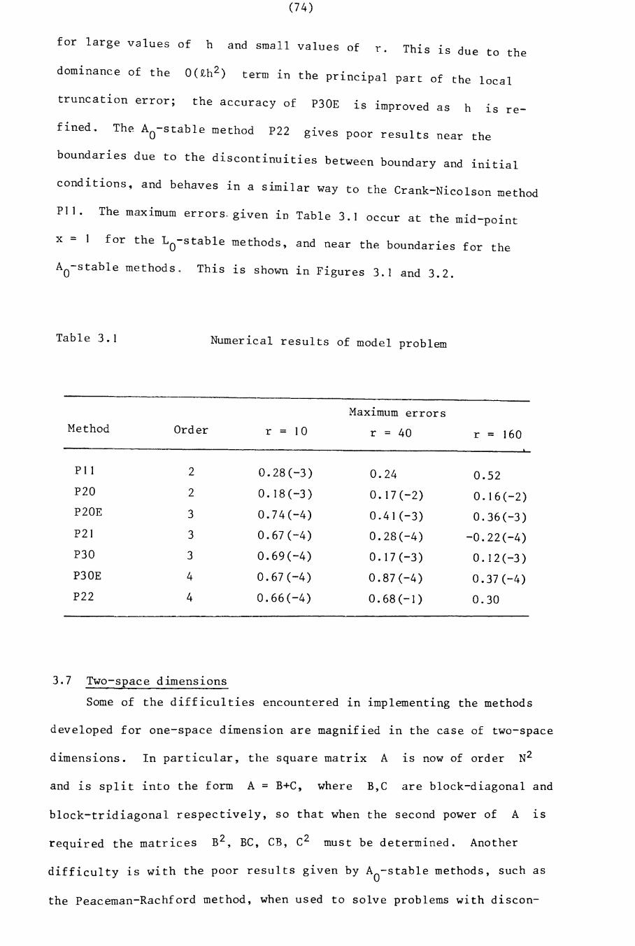
(74)
for large values of h and small values of r. This is due to the
dominance of the o(nh2) t . h .~ erm 1n t e pr1ncipal part of the local
truncation error; the accuracy of P30E is improved as h 1S re-
fined~
PI 1.
x = I
The Ao-stable method P22 g1ves poor results near the
boundaries due to the discontinuities between boundary and initial
conditions, and behaves in a similar way to the Crank-Nicolson method
The maximum errors. given in Table 3.1 h'occur at t e m1d-point
for the Lo-stable methods, and near the boundaries for the
Ao-stable methods. This is shown in Figures 3.1 and 3.2.
Table 3.1 Numerical results of model problem
Maximum errorsMethod Order r = 10 r = 40 r = 160
P I I 2 0.28(-3) 0.24 0.52P20 2 0.18(-3) 0.17(-2) 0.16(-2)P20E 3 0.74(-4) 0.41(-3) 0.36(-3)P21 3 0.67(-4) 0.28(-4) -0.22(-4)P30 3 0.69(-4) 0.17(-3) O. 12(-3)P30E 4 0.67(-4) 0.87(-4) 0.37 (-4)P22 4 0.66(-4) 0.68 (-I) 0.30
3.7 Two-space dimensions
Some of the difficulties encountered in implementing the methods
developed for one-space dimension are magnified in the case of two-space
dimensions. In particular, the square matrix A is now of order N2
and is split into the form A = B+C, where B,C are block-diagonal and
block-tridiagonal respectively, so that when the second power of A 1S
required the matrices B2 , BC, CB, C2 must be determined. Another
difficulty is with the poor results given by Ao-stable methods, such as
the Peaceman-Rachford method, when used to solve problems with discon-
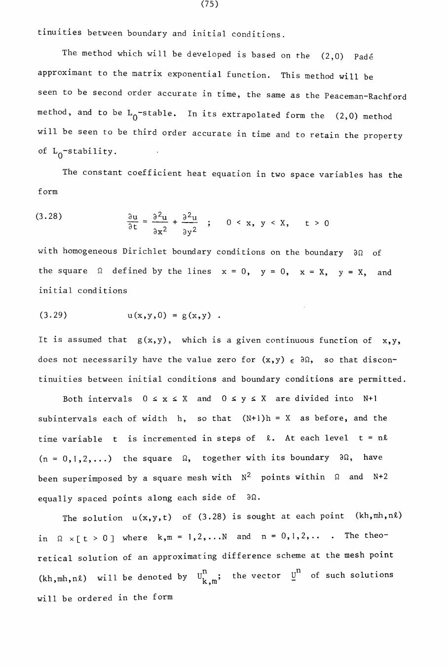
(75)
tinuities between boundary and initial conditions.
The method which will be developed is based on the (2,0) Pade
approximant to the matrix exponential function. This method will be
seen to be second order accurate in time, the same as the Peaceman-Rachford
method, and to be Lo-stable. In its extrapolated form the (2,0) method
will be seen to be third order accurate in time and to retain the property
of Lo-stability.
The constant coefficient heat equation ~n two space variables has the
form
(3.28 ) auat
., o < x, Y < x, t > 0
with homogeneous Dirichlet boundary conditions on the boundary an of
the square n defined by the lines x = 0, y = 0, x = X, Y = X, and
initial conditions
(3.29) u(x,y,O) = g(x,y) .
The theo-
It is assumed that g(x,y), which is a g~ven continuous function of x,y,
does not necessarily have the value zero for (x,y) E an, so that discon-
tinuities between initial conditions and boundary conditions are permitted.
Both intervals 0 ~ x ~ X and 0 ~ y ~ X are divided into N+1
subintervals each of width h, so that (N+1)h = X as before, and the
time variable t ~s incremented ~n steps of i. At each level t = ni
(n = 0,1,2, ... ) the square n, together with its boundary an, have
been superimposed by a square mesh with N2 points within nand N+2
equally spaced points along each side of an.
The solution u(x,y,t) of (3.28) ~s sought at each point (kh,mh,ni)
inn x [t > 0 ] where k , m = 1, 2, . . . Nand n = 0, 1, 2, . .
retical solution of an approximating difference scheme at the mesh point
(kh,mh,n£) will be denoted byn
Uk ;,mthe vector Un of such solutions
will be ordered in the form
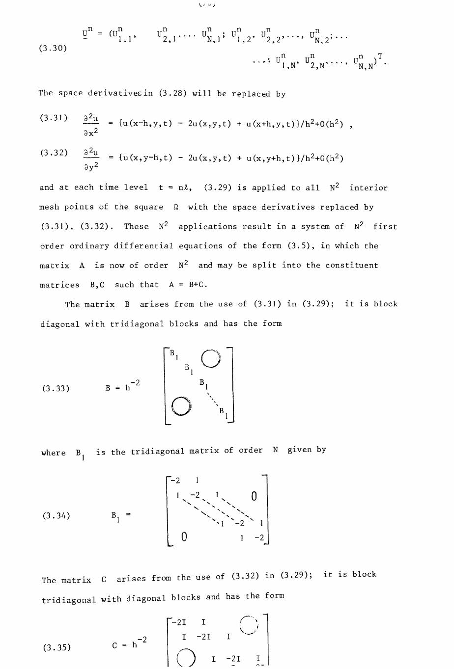
n(D 1• 1 ~
(3.30)un Un Un)T
I,N' 2,N"'" N,N •
The space derivativesin (3.28) will be replaced by
(3.31 )
(3.32)
a2u-- =
ax2
a2u=
ay2
{u(x-h,y,t) - 2u(x,y,t) + u(x+h,y,t)}/h2+O(h2 ) ,
{u(x,y-h,t) - 2u(x,y,t) + u(x,y+h,t)}/h2+O(h2 )
and at each time level t = nt, (3.29) is applied to all N2 interior
mesh points of the square n with the space derivatives replaced by
(3.31), (3.32). These N2 applications result in a system of N2 first
order ordinary differential equations of the form (3.5), in which the
mat~ix A is now of order N2 and may be split into the constituent
matrices B,C such that A = B+C"
The matrix B arises from the use of (3.31) In (3.29); it lS block
diagonal with tridiagonal blocks and has the form
B} 0B1
(3" 33)-2 B1B = h ,
0,,,,
B1
where B} lS the tridiagonal matrix of order N glven by
(3.34 )
-2
a
-2" "
o
-2
The matrix C arlses from the use of (3.32) In (3.29); it lS block
'd' I wl"th dl"agonal blocks and has the formtrl lagona
/'-'-'-"
-21 I t "r I-....}
-2 I -21 I
(3.35 ) C = h
() I -21 I
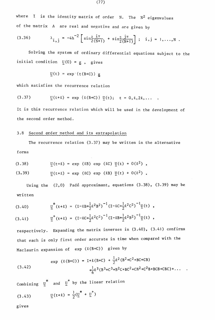
(77)
where I 1S the identity matrix of order N. The N2 eigenvalues
of the matrix A are real and negative and are given by
(3.36) A•• = -4h-2 [sin2 i7T + . 2 J7T ] ..1, J 2 (N+ 1) s 1n2 (N+ 1) ; 1, J = 1, ... , N .
Solving the system of ordinary differential equations subject to the
initial condition ~(o) = g , .g1ves
~(t) = exp"{t(B+C)} g
which satisfies the recurrence relation
(3 .37 ) ~(t+£) = exp {£(B+C)} ~(t); t = 0,£,2£, ...
It is this recurrence relation which will be used in the development of
the second order method.
3.8 Second order method and its extrapolation
The recurrence relation (3.37) may be written 1n the alternative
forms
(3.38) ~(t+£) = exp (£B) exp (£C) U(t) + 0(£2)
(3.39) ~(t+£) = exp (£C) exp (£B) ~(t) + 0(£2)
Using the (2,0) Pade approximant, equations (3.38), (3.39) may be
written
(3.40)
(3.41)
~*(t+£) = (I-£B+}£2B2)-1(I-£C+I£2C2)-1~(t) ,
+ 1 -1 1 2 2 -1U (t+£) = (I-£C+z£2C 2) (I-£B+z£ B) !:!(t) ,
respectively. Expanding the matrix inverses in (3.40), (3.41) confirms
that each is only first order accurate in time when compared with the
Maclaurin expansion of exp (£(B+C» given by
(3.42)
exp (£(B+C» = I+£(B+C) + ~£2(B2+C2+BC+CB)
~£3(B3+C3+B2C+BC2+CR2+C2B+BCB+CBC)+ ...6
* d U+ by the linear relationCombining U an
(3.43) U(t+£)
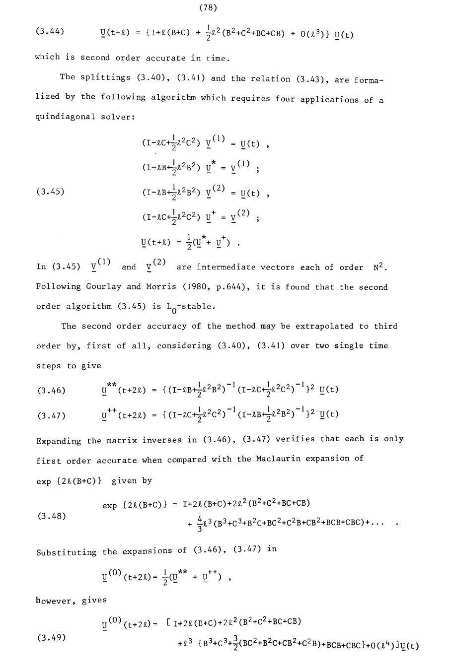
(78)
(3.44)
which is second order accurate ~n time.
The splittings (3.40), (3.41) and the relation (3.43), are forma-
lized by the following algorithm which requires four applications of a
quindiagonal solver:
(I-£B~£2B2) u* =...
(3.45) (I-£B~£2B2) V(2) = U_(t) ,2 -
(I-£C~£2C2) U+ = V(2)2 - -
1 * +~(t+£) = 2(~ + ~ ) .
In (3.45) Vel) and V(2) are intermediate vectors each of order N2.
Following Gourlay and Morris (1980, p.644), it is found that the second
order algorithm (3.45) is Lo-stable.
The second order accuracy of the method may be extrapolated to third
order by, first of all, considering (3.40), (3.41) over two single time
.steps to g~ve
(3 .46)
(3.47 )
**U (t+2£)
++!:! (t+2£)
= {(I-£B~£2B2)-1(I-£C~£2C2)-1}2 U(t)22-
= {(I_£C~£2C2)-1(I-£B~£2B2)-1}2 U(t)22-
Expanding the matrix inverses in (3.46), (3.47) verifies that each ~s only
first order accurate when compared with the Maclaurin expansion of
exp {2£(B+C)} g~ven by
exp {2£(B+C)}(3.48 )
= I+2£(B+C)+2£2(B 2+C 2+BC+CB)
+ ~£3(B3+C3+B2C+BC2+C2B+CB2+BCB+CBC)+ ...3
Substituting the expansions of (3.46), (3.47) ~n
however, gives
(3.49)
U(0)(t+2£)= [I+2£(n+C)+2~2(B2+C2+BC+CB)
+£3 {B3+C3+?(BC2+B2C+CB2+C2B)+BCB+CBC}+0(£4)J~(t)
showing that U(O)
(79)
1S second order accurate 1n time.
Writing (5.40), (5.41) over a double time step 2£ glves
(3.50)
(3.51)
~(1)(t+2£) = (I-2£B+2£2B2)-I(I-2£C+2£2C2)-I~(t) ,
~(2)(t+2£) = (I-2£C+2£2C 2)-1 (I-2£B+2£2B2)-I U(t)
Expanding the matrix 1nverses 1n (3.50), (3.51) glves
(3.52)
(3.53 )
~(1)(t+2£) = {I+2£(B+C)+2£2(B2+C2+2BC)
+ 4£3(B2C+BC2)+0(£4)}~(t) ,
~(2)(t+2£) = {I+2£(B+C)+2£2(B2+C2+2CB)
+ 4£3(C2B+CB2)+0(£4)}~(t)
respectively, showing that each is first order accurate in time.
The linear combination of (3.49), (3.52), (3.53), defined by
1S third order accurate in time when compared with the Maclaurin
expansion (3.48).
The principal part of the local truncation error of (3.43) when
applied to the mesh points (kh,mh,n£), with k,m = 2, ... ,N-I and
n = 0,1,2, ... , 1S found to be
(3.54 ) (~£3o3u _1_£h2 ( 04u + 04u) ) n k,m + 1,N-- -
6 ot 3 12 ox4 oy4 k,m
which, following extrapolation, becomes
(3.55 ) ., k,m + I,N
The implementation of the algorithm based on the (2,0) Pade
approximant may be carried out by means of the following strategy:
(i) intermediate vectors are introduced and used to
* +find the estimates U (t+£). U (t+£), as follows:
(3.56)
(3.57)
(I-£C+}£2C2) ~(I)= ~(t)
1 * (1)(I-£B~£2B2) ~ (t+£) = ~
(3.58 )
(3.59)
(80)
(I-£B~£2B2) V(2) = U(t)2 - _
(I-£C+~£2C2) ~+(t+i) = v(2)
intermediate vectors(ii)
the estimates
follows:
*~ (t+i), +~ (t+i)
are introduced to extend
over a second single time step as
(3.60) ,
(3.61)
(3.62)
(3.63)
(iii)
(I-iB~i2B2) ~**(t+2i) = y(3)
(I-£B~£2B2) y(4)= ~+(t+i)
(I-£C+}i2C 2) U++(t+2i) = v(4)
the second order estimate U(O)~s now calculated from
(3.64)
(iv)
U(0) 1 (U** ++= - + U )- 2 - -
intermediate vectors
.,
V(5)- , are introduced and used
with a double time step to find the estimates ~(I)(t+2i) and
u(2)(t+2i) as follows:
(3.65) (I-2iC+2i2C 2) y(5) = ~(t)
(3.66 ) (I-2iB+2i2B 2) ~(I)(t+2i) = y(5) .,
(3.67 ) (I-2iB+2i2B2) y(6) = ~(t)
(3.68 ) (I-2iC+2i2C 2) ~(2)(t+2i) = y(6) .,
(v) the third order accurate estimate U(E) (t+22)g~ven by- ,
(3.69 ) ~(E)(t+2i) = i U(O) _ ..!-(u(I)+ u(2»3 - 6 - - ,
is now calculated.
In order to illustrate the behaviours of the La-stable methods in
two space variables, the following model problem, which was introduced
in the paper by Lawson and Morris (1978), is solved using the second
order method (3.45), and third order method as an extrapolation of the
second order method.
The problem is
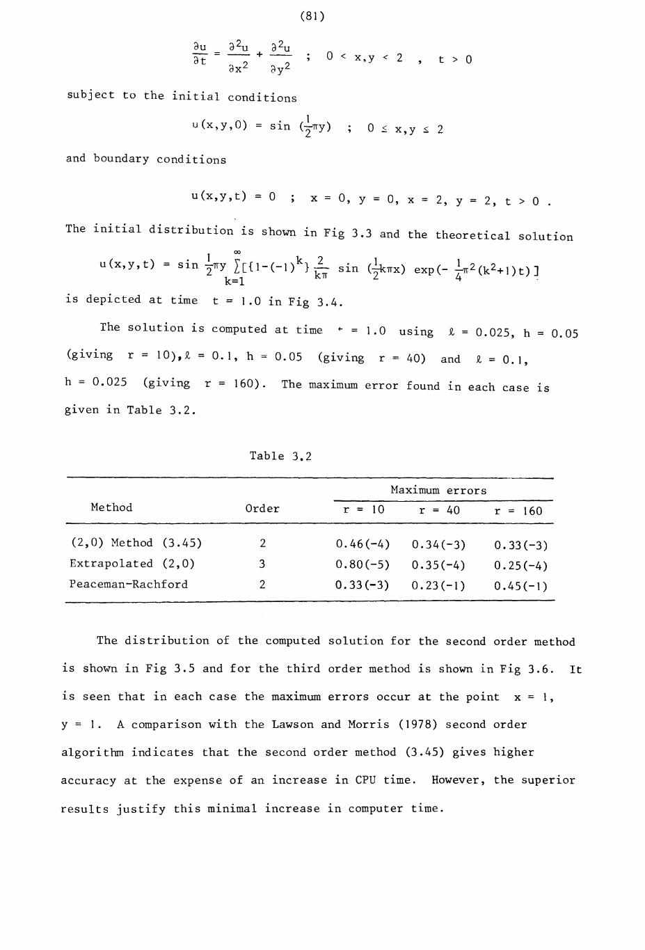
dUdt = -- +
(81 )
o < x,y < 2 t > 0
subject to the initial conditions
u(x,y,O) = sln
and boundary conditions
., o .:s: x,y ~ 2
u(x,y,t) = 0 x = 0, y = 0, x = 2, y = 2, t > 0 .
u(x,y,t)
The initial distribution is shown 1n Fig 3.3 and the theoretical solution
00
1 \ k 2 1 1= s i.n I 7fy L[{I-(-I) }-k sin (71<27fx) exp(- -7f2 (k 2+1)t)]
k=l n 4.
1S depicted at time t = 1.0 in Fig 3.4.
The solution is computed at time ~ = 1.0 uS1ng i = 0.025, h = 0.05
(giving r = 10),i = 0.1, h = 0.05 (giving r = 40) and i = 0.1,
h = 0.025 (giving r = 160). The maX1mum error found in each case 1S
given in Table 3.2.
Table 3.2
Maximum errorsMethod Order r = 10 r = 40 r = 160
(2,0) Method (3.45) 2 0.46(-4) 0.34(-3) 0.33(-3)
Extrapolated (2,0) 3 0.80(-5) 0.35(-4) 0.25(-4)
Peaceman-Rachford 2 0.33(-3) 0.23 (-1 ) 0.45(-1)
The distribution of the computed solution for the second order method
1S shown in Fig 3.5 and for the third order method 1S shown in Fig 3.6. It
1S seen that in each case the maximum errors occur at the point x = 1,
y = 1. A comparison with the Lawson and Morris (1978) second order
algorithm indicates that the second order method (3.45) gives higher
accuracy at the expense of an increase in CPU time. However, the superior
results justify this minimal increase in computer time.
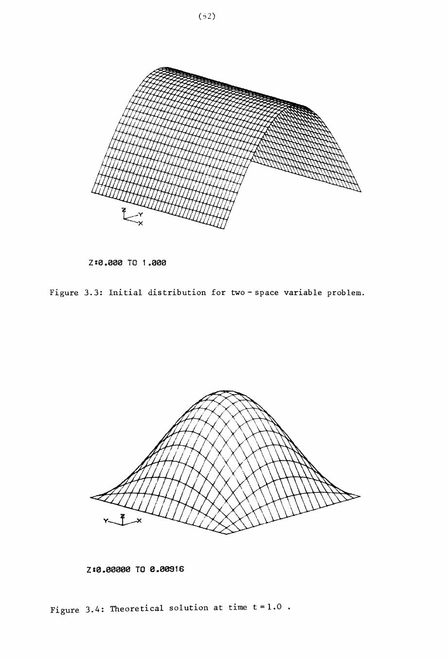
( ~2)
Z:0.000 TO 1 .000
Figure 3.3: lni tial dis tribution for two - space variab Le prob lem.
Z:0.00000 TO 0.00916
Figure 3.4: Theoretical solution at time t = 1.0 •
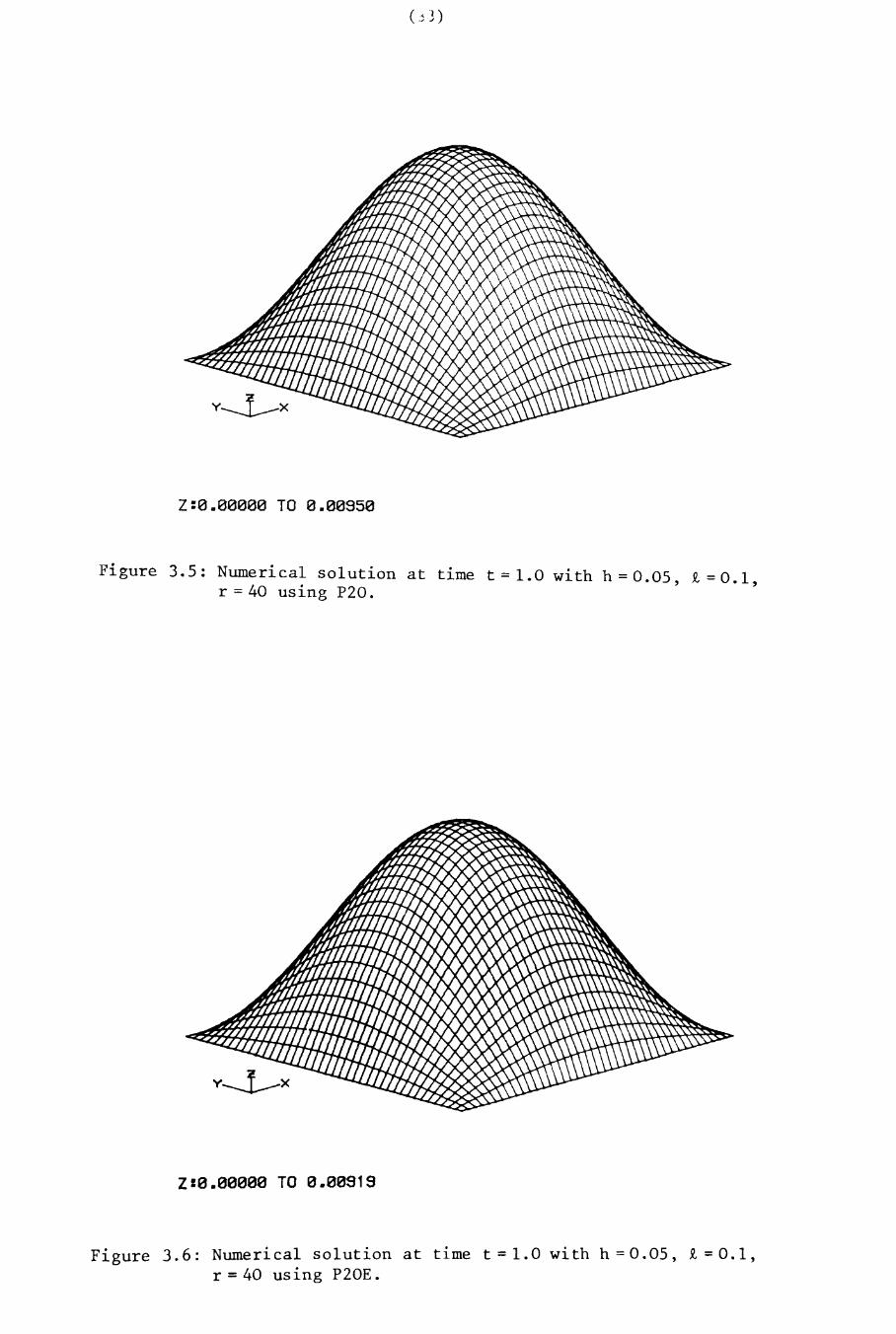
Z:0.00000 TO 0.00950
Figure 3.5: Numerical solution at time t=l.O with h=0.05, £=0.1,r = 40 using P20.
Z:0.00000 TO 0.00919
Figure 3.6: Numerical solution at time t=l.O with h=0.05, £=0.1,r = 40 using P20E.
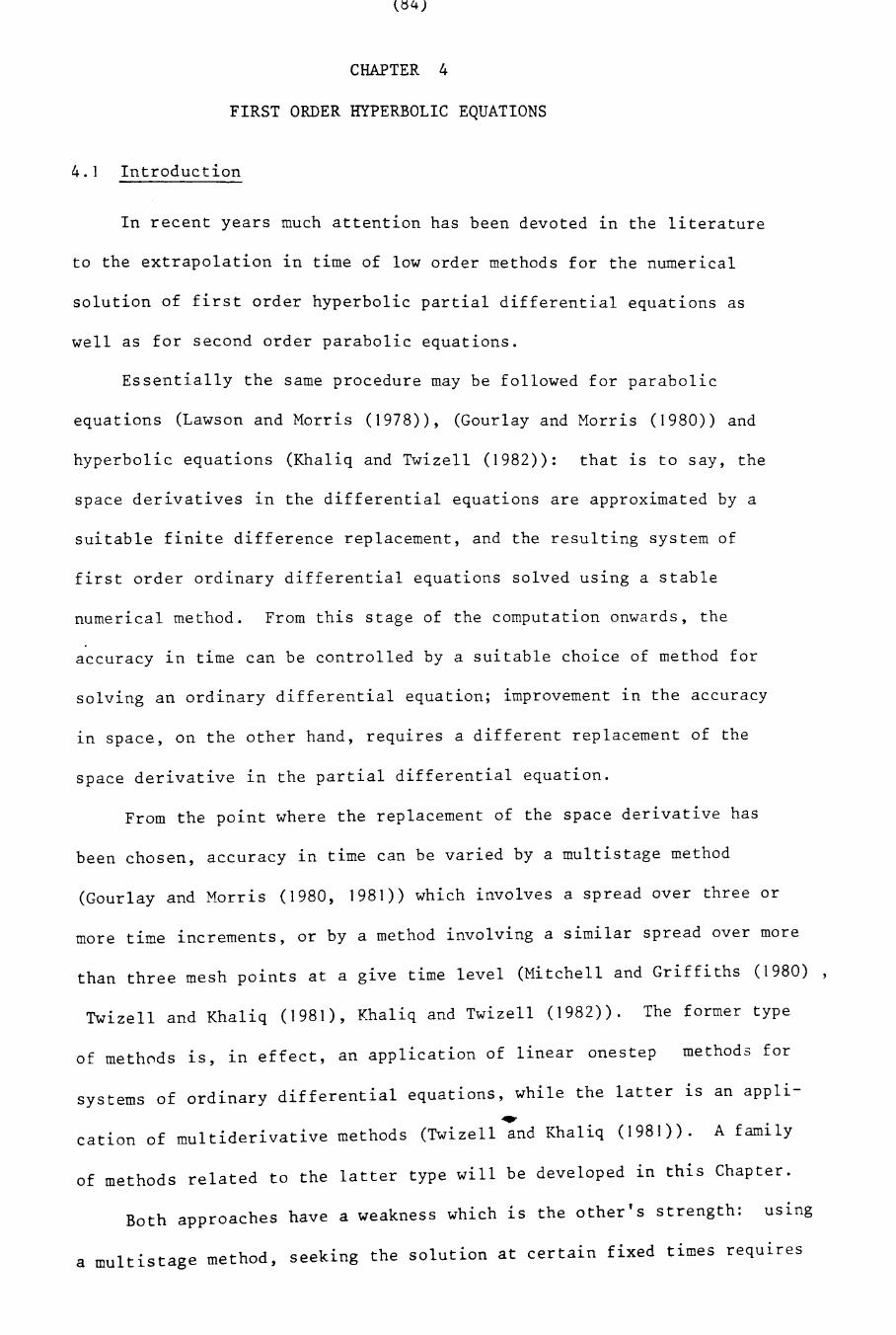
t~4)
CHAPTER 4
FIRST ORDER HYPERBOLIC EQUATIONS
4.1 Introduction
In recent years much attention has been devoted in the literature
to the extrapolation ln time of low order methods for the numerical
solution of first order hyperbolic partial differential equations as
well as for second order parabolic equations.
Essentially the same procedure may be followed for parabolic
equations (Lawson and Morris (1978)), (Gourlay and Morris (1980)) and
hyperbolic equations (Khaliq and Twizell (1982)): that is to say, the
space derivatives in the differential equations are approximated by a
suitable finite difference replacement, and the resulting system of
first order ordinary differential equations solved using a stable
numerical method. From this stage of the computation onwards, the
accuracy in time can be controlled by a suitable choice of method for
solving an ordinary differential equation; improvement in the accuracy
in space, on the other hand, requires a different replacement of the
space derivative in the partial differential equation.
From the point where the replacement of the space derivative has
been chosen, accuracy in time can be varied by a multistage method
(Gourlay and Morris (1980, 1981)) which involves a spread over three or
more time increments, or by a method involving a similar spread over more
than three mesh points at a give time level (Mitchell and Griffiths (1980) ,
Twizell and Khaliq (1981), Khaliq and Twizell (1982)). The former type
of methods is, in effect, an application of linear onestep methods for
systems of ordinary differential equations, while the latter 1S an appli~
cation of multiderivative methods (Twizell and Khaliq (1981)). A family
of methods related to the latter type will be developed in this Chapter.
Both approaches have a weakness which 1S the other's strength: uS1ng
a multistage method, seeking the solution at certain fixed times requ1res
(85)
the time interval to be divided into two or more subintervals depending
upon the accuracy required, whereas the integration can be carried out
without subdividing the time interval if an A-stable or L-stable multi
derivative method is used. On the other hand, implicit multistage
methods need only tridiagonal solvers to obtain the solution (five at
each time level for third order accuracy in time and nine for fourth
order accuracy (Gourlay 'and Morris (1980)), whereas the multiderivative
methods in Chapter 3, based on central difference replacements of the
space derivative, (Khaliq and Twizell (1982)), need quindiagonal or
seven diagonal solvers.
The methods to be discussed 1n sections 4.3, 4.4, 4.5, are based
on backward difference replacements of the space derivatives and can
therefore be used explicitly so that here, too, they have an advantage
over multistage formulations. The use of backward difference replace
ments has the advantage that the oscillations which are always present
with central difference replacements (section 4.2), do not arise. Also
the difficulties which arise in parabolic equations because of stiffness
are not present in solving hyperbolic equations by multiderivative
techniques. The methods will use function values at only two time levels
as in Khaliq and Twizell (1982), unlike the methods developed by Oliger
(1974), and depend on the theorems of Gustaffson (1972) for the establish
ment of stability. The methods are tested in section 4.6 on a number of
problems from the literature and, finally, conclusions are drawn in
section 4.7.
(86)
4.2 Central difference approximation in space
Consider the first order hyperbolic partial differential equation
(4. I ) au + eluat a ax = ° a > 0, x > 0, t > ° ,
where a lS a constant, with initial conditions
(4.2) u(x,O) = g(x)X ~ °
and boundary conditions
(4.3) u(O,t) = vet) ., t > °equations (4.1), (4.2), (4.3) form the initial-boundary value problem.
Suppose that the solution of (4.1) is sought in some region R =[0 < x < XJ x
[t > OJ of the first quarter plane x > 0, t > ° (out flow problem). The
interval ° ~ x ~ X is divided into N equal parts each of width h, so
that Nh = X, and the time variable t is discretized in steps of length
£. The open reglon R and its boundary aR, consisting of the axes
t = 0, x = ° and the line x = X, have been covered by a rectangular
mesh, the mesh points having co-ordinates (mh,ni) where m = O,I, ... ,N
and n = 0, 1, 2, ... The theoretical solution of a finite difference
scheme approximating the differential equation at this point, will be
denoted by un ::: U(mh,n£).m
Replacing the space derivative In (4.1) by the central difference
formula
(4.4) ~~ =[u(x+h,t) - u(x-h,t)Y2h + 0(h2 ) ,
and applying (4.1) with (4.4), (4.2), (4.3) to all N interior mesh
. . I I t n ( - ° 1 ) leads to the system of firstpOlnts at tlme eve = nN n - , , ... ,
order ordinary differential equations
(4.5) dU--dt1
+ -aw2 -t
Twhere ~(t) =[U1(t), U2(t), ... , UN(t)J , T denoting transpose, is the
vector of approximate solutions of (4.1) at time t > 0. In (4.5) B lS
a square matrix of order N glven by
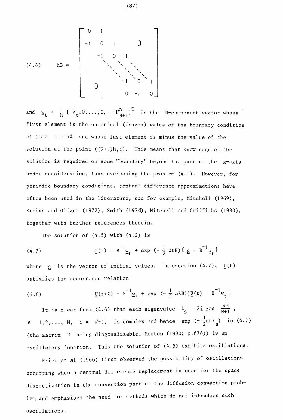
(87)
°-I ° o
°(4.6) hB =
-1" , ,, , ,, , ,, , ,, ,, ,
-1 '0 'o
° -1 0
and1
~t = h [vt'O, ... ,O, 1.8 the N-component vector whose
first element is the numerical (frozen) value of the boundary condition
at time t = n£ and whose last element is minus the value of the
solution at the point «N+l)h,t). This means that knowledge of the
solu tion 1.S required on some "boundary" beyond the part of the x-<axas
under consideration, thus overposing the problem (4.1). However, for
periodic boundary conditions, central difference approximations have
often been used in the literature, see for example, Mitchell (1969),
Kreiss and Oliger (1972), Smith (1978), Mitchell and Griffiths (1980),
together with further references therein.
The solution of (4.5) with (4.2) 1.S
(4.7)-1 1 -1
~(t) = B ~t + exp (- 2 atB){ g - B ~t}
where g 1.S the vector of initial values. In equation (4.7), ~(t)
satisfies the recurrence relation
(4.8)-1 1 -1
~(t+£) = B ~t + exp (- 2" a£B){~(t) - B ~t}
It is clear from (4.6) that each eigenvalue
s= 1,2, ... , N, 1. = Ff, is complex and hence
As = 2i cos
1exp (- 2"atA
s)
S1r
N+ 1 '
1.n (4.7)
(the matrix B being diagonalizable, Morton (1980; p.678)) 1.S an
oscillatory function. Thus the solution of (4.5) exhibits oscillations.
Price et al (1966) first observed the possibility of oscillations
occurring when a central difference replacement is used for the space
discretization in the convection part of the diffusion-convection prob-
lem and emphasised the need for methods which do not introduce such
oscillations.
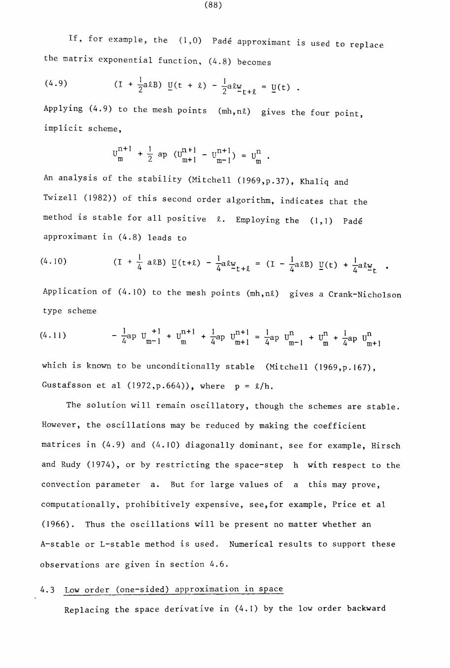
(88)
If, for example, the (1~0) Pade approximant 1S used to replace
the matrix exponential function, (4.8) becomes
(4.9) 1 1(I + -2atB) ~(t + t) - -atw = U_(t)
2 -t+t
Applying (4.9) to the mesh points (mh,nt) glves the four point,
implicit scheme,
n+ 1 1 n +-1 n+ 1 nU + - ap (U - U ) = U .
m 2 m+l m-l m
An analysis of the stability (Mitchell (1969,p.37), Khaliq and
Twizell (1982» of this second order algorithm, indicates that the
method is stable for all positive t. Employing the (1,1) Pade
approximant in (4.8) leads to
(4.10) 1 1(I + -4- atB) ~(t+t) - -atw
4 -t+t
Application of (4.10) to the mesh points (mh,nt) glves a Crank-Nicholson
type scheme
(4.11 ) - !ap U +1 + Un+ 1 + !ap Un+ 1 =4 m-l m 4 m+l
which is known to be unconditionally stable (Mitchell (1969,p.167),
Gustafsson et al (1972,p.664», where p = t/h.
The solution will remain oscillatory, though the schemes are stable.
However, the oscillations may be reduced by making the coefficient
matrices in (4.9) and (4.10) diagonally dominant, see for example, Hirsch
and Rudy (1974), or by restricting the space-step h with respect to the
convection parameter a. But for large values of a this may prove,
computationally, prohibitively expensive, see,for example, Price et al
(1966). Thus the oscillations will be present no matter whether an
A-stable or L-stable method is used. Numerical results to support these
observations are given in section 4.6.
4.3 Low order (one-sided) approximation 1n space
Replacing the space derivative in (4.1) by the low order backward
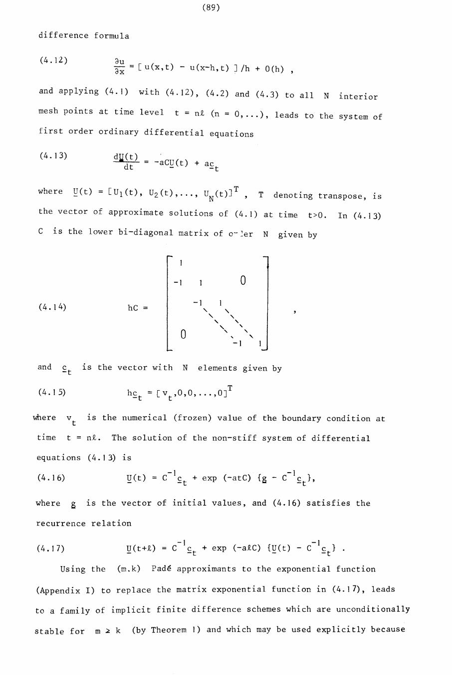
(89)
difference formula
(4.12) auax = [u(x,t) - u(x-h,t) J/h + O(h) ,
and applying (4. 1) with (4.12), (4.2) and (4.3) to all N interior
mesh points at time level t = n£ (n = 0, ... ) , leads to the system of
first order ordinary differential equations
(4. 13)~=
dt -aC~(t) + ac-t
T denoting transpose, is
the vector of approximate solutions of (4.1) at time t>O. In (4.13)
C is the lower bi-diagonal matrix of o'~~er N glven by
-1 o
,
,-1
1\.
"",""
-1-,
-,
"-,,o
hC =(4.14)
and £t 1S the vector with N elements glven by
(4. 1 5) hc-t
T= [v ,0,0, ... ,OJt
where v 1S the numerical (frozen) value of the boundary condition att
time t = n£. The solution of the non-stiff system of differential
equations (4.13) 1S
(4.16)-1 -1
~(t) = C £t + exp (-atC) {g - C £t}'
where g 1S the vector of initial values, and (4.16) satisfies the
recurrence relation
(4.17)
Using the (m.k) Pad~ approximants to the exponential function
(Appendix I) to replace the matrix exponential function in (4.17), leads
to a family of implicit finite difference schemes which are unconditionally
stable for m ~ k (by Theorem 1) and which may be used explicitly because
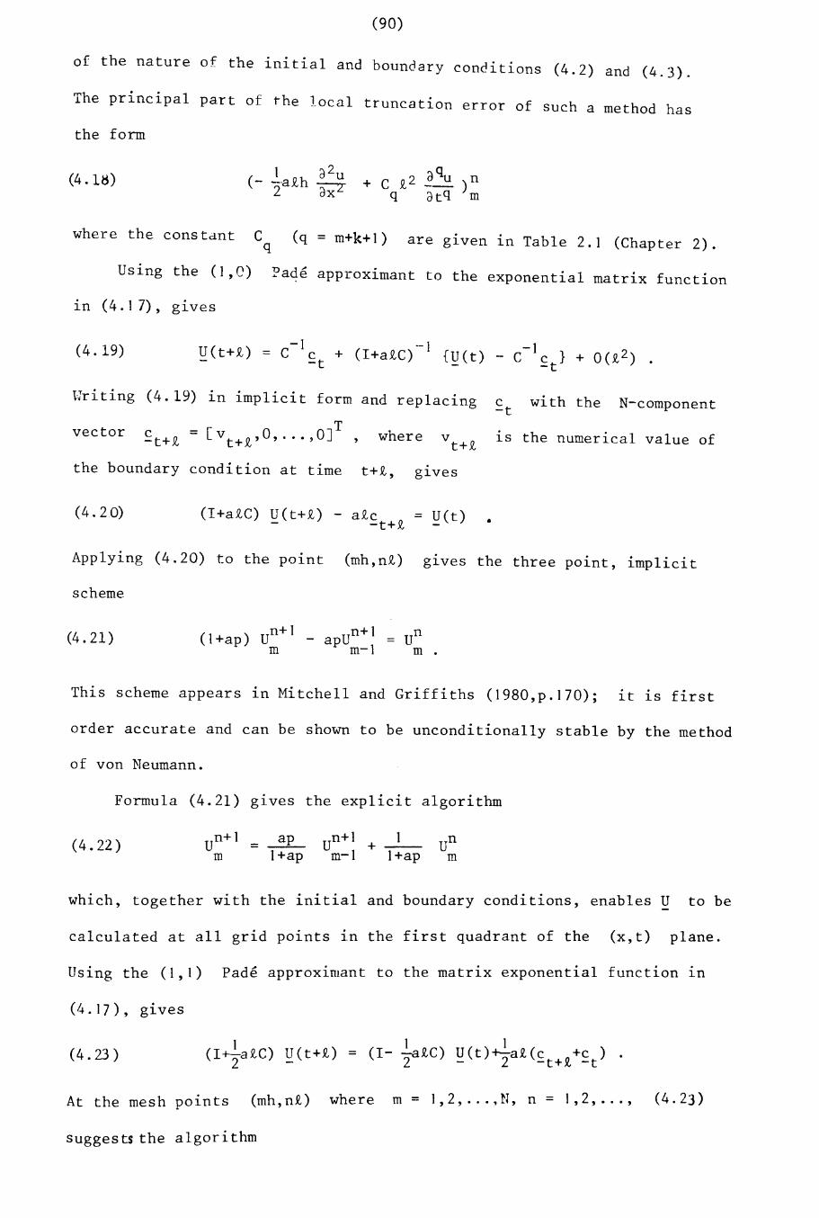
(90)
of the nature of the initial and boundary concitions (4.2) d (4 3)an ..
The principal part of the local truncation error of such a method has
the form
(4. un
where the constant Cq
(q = m+k+I) .are glven 1n Table 2.1 (Chapter 2).
Using the (1,0) Pade approximant to the exponential matrix function
t n (4. 1 7) ,
(4. 19)
N-component
1S the numerical value of
c with the-t
v t+sz'where
Writing (4.19) 1n implicit form and replacing
T£t+sz' = [vt+SZ"O, ... ,OJvector
the boundary condition at time t+sz', glves
(4.20) (I+aSZ,C) ~(t+sz') - asz'c = U_(t)-t+sz' •
Applying (4.20) to the point (mh,nsz') glves the three point, implicit
scheme
(4.21 ) n+I n+I n(I+ap) U - apU = Um m-I m.
This scheme appears in Mitchell and Griffiths (I980,p.I70); it 1S first
order accurate and can be shown to be unconditionally stable by the method
of von Neumann.
Formula (4.21) glves the explicit algorithm
(4.22 ) n+IU
m= ap
I+apUn+I + _1_
m-I I+ap
which, together with the initial and boundary conditions, enables U to be
calculated at all grid points in the first quadrant of the (x,t) plane.
Using the (1,1) Pade approxinlant to the matrix exponential function in
(4.17), gives
(4.23)
At the mesh points (mhvn t ) where m = 1,2, ... ,N, n = 1,2, •.. , (4.23)
suggests the algorithm
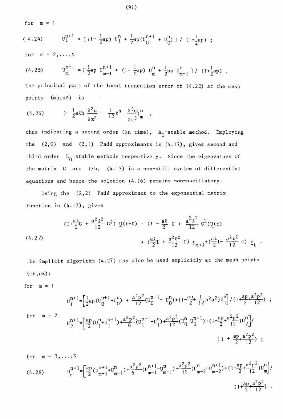
(91)
for m =
( 4.24)
for m = 2, ... ,N
(4.25) n+ 1 1 n+lIn 1 1U = [-ap U + (1- -ap) U + -ap Un ] I (1+-2ap) .
m 2 rrr-12m 2 nr-J
The principal part of the local truncation error of (4.23) at the mesh
points (mh, n z ) 1S
(4.26) (-I a2u _1_£3 a 3u n-a£h -- - -)2 ax2 12 at 3 m
,
thus indicating a second order (in time), Ao- s t ab1e method. Employing
the (2,0) and (2,1) Pade approximants 1n (4.17), gives second and
third order Lo-stab1e methods respectively. Since the eigenvalues of
the matrix Care Ilh, (4.13) is a non-stiff system of differential
equations and hence the solution (4.16) rema1ns non-oscillatory.
Using the (2,2) Pade approximant to the exponential matrix
function in (4.17), glves
(r~ +a2 £2
C2) !:!(t+£) = (r - a£ C +a 2£2
C2)U(t)--2 12 2 12
(4.27) (a£r + a 2£2C)
a£ a 2£2C)+
12c +(-r-
12c
2 -t+£ 2 -t
The implicit algorithm (4.27) may also be used explicitly at the mesh points
(mh,n£):
for m = 1
for m = 2
for m = 3, ... ,N
(4.28)
ap a2 p2( 1It)
2 12
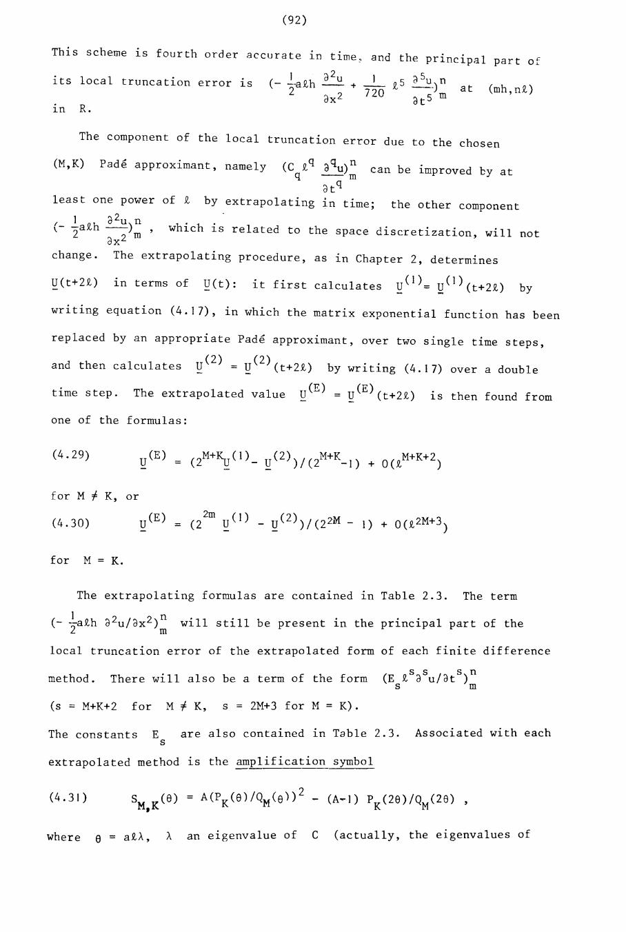
~n R.
(92)
This scheme is fourth order accurate in time~ and the principal part of
J a2 u 1 a5u nits local truncation error r s (- --a£h - + -- £5 --) at (rnh,n£)2 ax2 720 at S m
The component of the local truncation error due to the chosen
(M,K) Pade approximant, namely (C £q aqu)n can be improved by atq --m
Cltq
least one power of £ by extrapolating in time; the other component
(- ~a£h a2u)n,
which is related to the space discretization, will not2 "12m
oX
change. The extrapolating procedure, as in Chapter 2, determines
~(t+2£) in terms of ~(t): it first calculates ~(l)= Q(1)(t+2£) by
writing equation (4.17), in which the matrix exponential function has been
replaced by an appropriate Pade approximant, over two single time steps,
and then calculates ~(2) = ~(2)(t+2£) by
(E)time step. The extrapolated value U =
one of the formulas:
writing (4.17) over a double
~(E)(t+2£) ~s then found from
(4.29)
for M f K, or
(4.30)
for M = K.
The extrapolating formulas are contained in Table 2.3. The term
(- lath a 2u/ax2)n will still be present in the principal part of the2 m
local truncation error of the extrapolated form of each finite difference
method. There will also be a term of the form
(s = M+K+2 for M =I K, s = 2M+3 for M = K) •
The constants E are also contained ~n Table 2.3. Associated with eachs
extrapolated method ~s the amplification symbol
(4.31)
h 01 1 an eigenvalue of C (actually, the eigenvalues ofwere e = aJV/\, /\
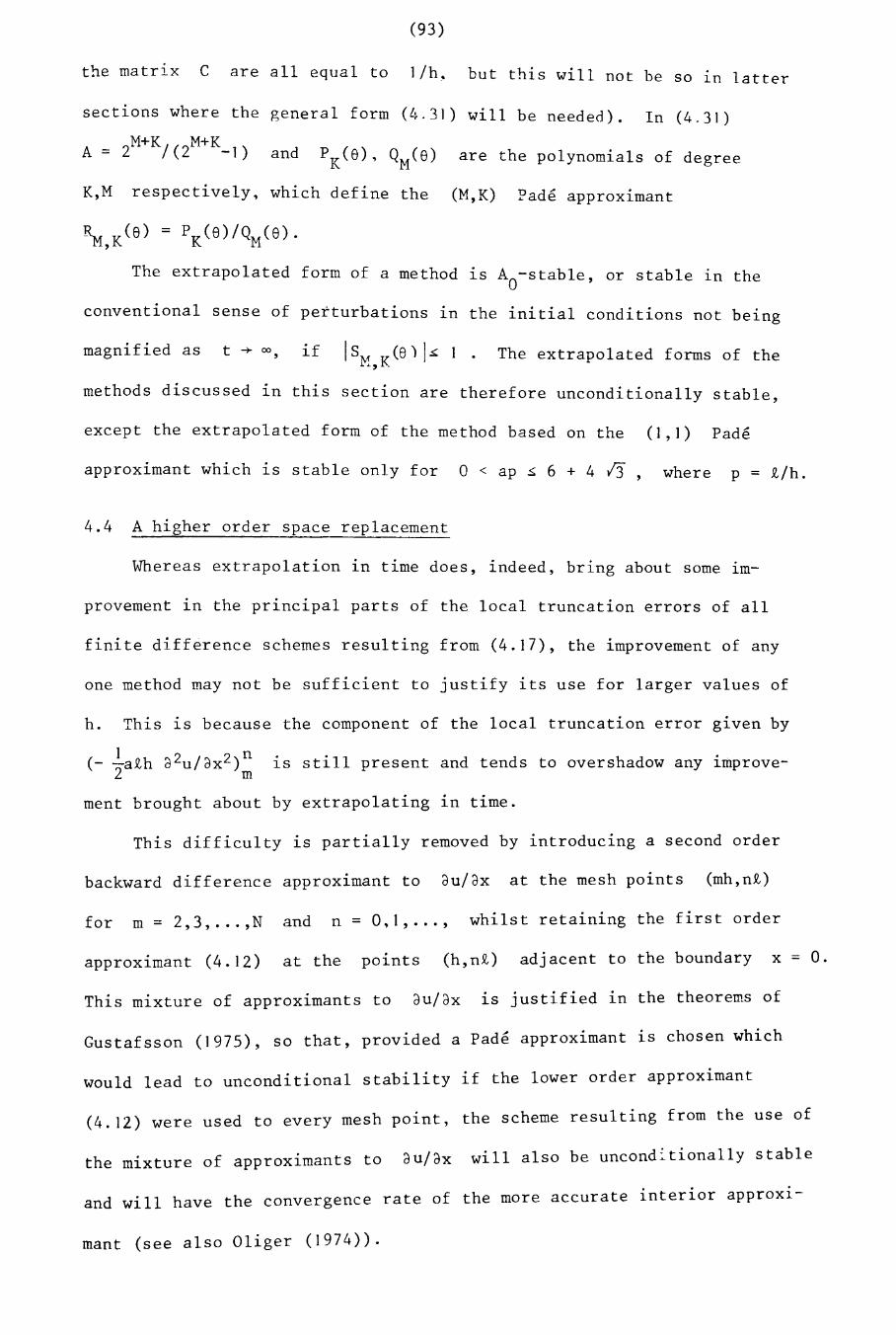
The extrapolated forms of the
(93)
the matrix C are all equal to l/h~ but this will not be so 1n latter
sections where the general form (L~.3J) will be needed). In (4.31)
A = 2M+K/(2M+K_l)and PK(8) , QM(8) are the polynomials of degree
K,M respectively, which define the (M,K) Pade approximant
The extrapolated form of a method 1S Ao-stable, or stable in the
conventional sense of perturbations in the initial conditions not being
magnified as t ~ 00, if ISM, K(8 ) I~ 1
methods discussed 1n this section are therefore unconditionally stable,
except the extrapolated form of the method based on the (1,1) Pade
approximant which is stable only for 0 < ap ~ 6 + 4 13, where p = £/h.
4.4 A higher order space replacement
Whereas extrapolation in time does, indeed, bring about some im-
provement in the principal parts of the local truncation errors of all
finite difference schemes resulting from (4.17), the improvement of any
one method may not be sufficient to justify its use for larger values of
h. This is because the component of the local truncation error g1ven by
(- !a£h a2u/ax2)n 1S still present and tends to overshadow any 1rnprove-2 m
ment brought about by extrapolating in time,
This difficulty is partially removed by introducing a second order
backward difference approximant to au/ax at the mesh points (mh,n£)
f 2 3 N d n - 0 I wh1'lst reta1'ning the first orderor m = " •.. , an -, " .. ,
approximant (4.12) at the points (h,n£) adjacent to the boundary x = o.
This mixture of approximants to au/ax 1S justified 1n the theorems of
Gustafsson (1975), so that, provided a Pade approximant is chosen which
would lead to unconditional stability if the lower order approximant
(4.12) were used to every mesh point, the scheme resulting from the use of
the mixture of approximants to au/ax will also be uncond:tiona11y stable
and will have the convergence rate of the more accurate interior approxi-
mant (see also Oliger (1974)).
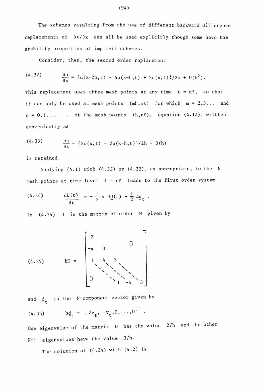
(94)
The schemes resulting from the use of different backward difference
replacements of au/ax can all be used explicitly though some have the
stability properties of implicit schemes.
Consider, then, the second order replacement
(4.32) auax = {u(x-2h,t) - 4u(x-h,t) + 3u(x,t)}/2h + 0(h2 ) .
This replacement uses three mesh points at any time t = nt, so that
it can only be used at mesh points (mh,n£) for which m = 2,3 ... and
n = 0,1, ...
conveniently as
At the mesh points (h,n£), equation (4.12), written
(4. 33)
1S retained.
auax
= {2u(x,t) - 2u(x-h,t)}/2h + O(h)
Applying (4.1) with (4.33) or (4.32), as appropriate, to the N
mesh points at time level t = n£ leads to the first order system
(4.34) dUet)
dt=
1 ]a DU_(t) + - ad2 2 -t
In (4.34) D 1S the matrix of order N g1ven by
2
0-4 3
(4.35) hD = -4 3"- "
,"- " ""- "-
,"-
, "0 "- <, "-"-
" 1 -4 3
and d-t
1S the N-component vector g1ven cy
(4.36)T
hd = [2v , -v ,0, ... , OJ .-t t t
. h h I 2/h and the otherOne eigenvalue of the matr1x D as t e va ue
N-] eigenvalues have the value 3/h.
The solution of (4.34) with (4.2) 1S
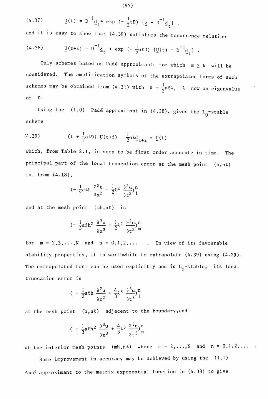
(4.37)
and it is
(4.38)
(95)
-1 1 -1~(t) = D ~t+ exp (- ~D) {g - D ~t} .
easy to show that (4.38) satisfies the recurrence relation
-1 1 1~(t+£) = D ~t + exp (- 2a £D) {~(t) - D- ~t} .
Only schemes based on Pade approximants for which m ~ k will be
considered. The amplification symbols of the extrapolated forms of such
schemes may be obtained from (4.31) with
of D.
1e = -a£>..2 ' now an eigenvalue
Using the (1,0) Pade approximant 1n (4.38), g1ves the La-stable
scheme
(4.39)
which, from Table 2.1, is seen to be first order accurate 1n time. The
principal part of the local truncation error at the mesh point (h,n~)
is, from (4.18),
1 ~2u _102 ~2u n(_ -a£h _0_ _ )(, _0_)2 ax2 2 at 2 1
and at the mesh point (mh,n£) 1S
for m = 2,3, ... ,N and n = 0,1,2, ... In V1ew of its favourable
stability properties, it is worthwhile to extrapolate (4.39) using (4.29).
The extrapolated form can be used explicitly and is La-stable; its local
truncation error 1S
1 a2u+ ~£3 a 3u n
( - -a£h -- -)2 ax 2 3 at 3 1
at the mesh point (h, nz ) adjacent to the boundary,and
at the interior mesh points (mh,n£) where m = 2, ... ,N and n = 0,1,2, ...
Some improvement in accuracy may be achieved by using the (1,1)
Pade approximant to the matrix exponential function in (4.38) to give
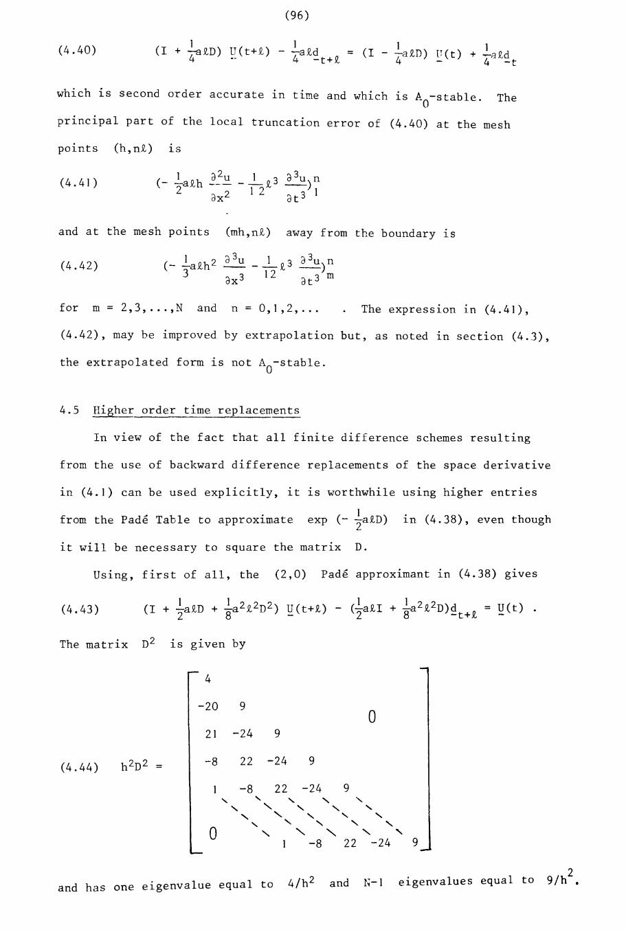
(4.40)
(96)
1 1(I + ~4£D) ~(t+£) - -a£d
4 -t+£1 1= (I - 4a£D) IT(t) + ~a£d
4 -t
which is second order accurate ~n time a d wh~ h· A t bln .LC r s 1"'-O-S a e. The
principal part of the local truncation error of (4.40) at the mesh
points (h,n£) ~s
(4.41)
and at the mesh points (mh,n£) away from the boundary ~s
(4.42) _1a Ilh 2 d 3u 1 a3u n(-:Iv __ £3 _)
3 dX 3 12 dt 3 m
for m = 2,3, ... ,N and n = 0,1,2, ... The express~on ~n (4.41),
(4.42), may be improved by extrapolation but, as noted in section (4.3),
the extrapolated form is not Ao-stable.
4.5 Higher order time replacements
In view of the fact that all finite difference schemes resulting
from the use of backward difference replacements of the space derivative
in (4.1) can be used explicitly, it is worthwhile us~ng higher entries
from the Pade Table to approximate1
exp (- Ia£D) in (4.38), even though
it will be necessary to square the matrix D.
Using, first of all, the (2,0) Pade approximant ~n (4.38) g~ves
(4.43)
The matrix D2~s g~ven by
4
-20 90
21 -24 9
(4.44) h 2D2 = -8 22 -24 9
-8 22 -24 9"- "- "- <, <,
"<, " <, "-
<, <, <, "- <,
"- " <, <, <,
0 -, <, <, <, <,
-8 22 -24 9
4/h 2 d 1\' 1 e i.ge nva lue s equal to 9/h2•
and has one eigenvalue equal to an 1~- .L
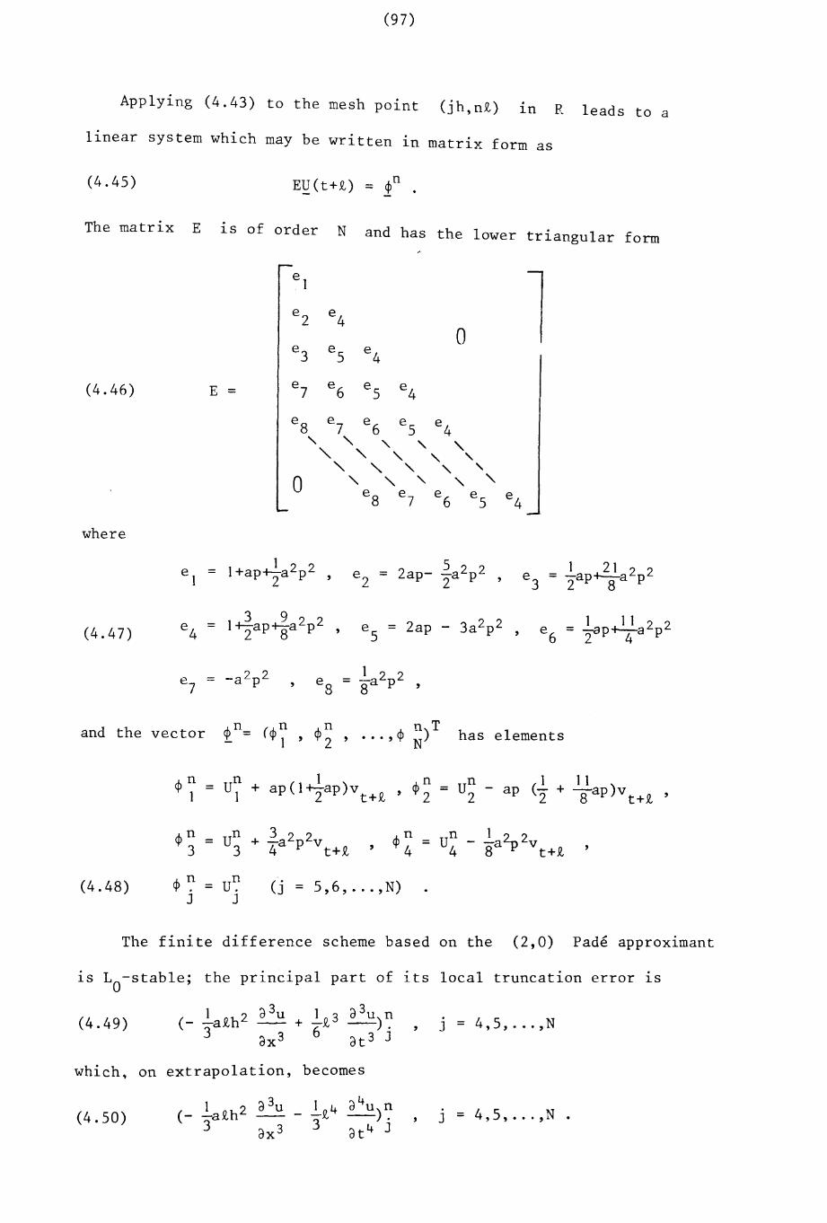
(97)
Applying (4.43) to the mesh point (jh~n£) 1n R leads to a
linear system which may be written in matrix form as
(4.45) E!:!(t+£) = ¢n .
The matrix E 1S of order N and has the lower triangular form
e 1
le2 e
40e
3 e5 e
4
(4.46) E = e7 e6 e
5 e4
eS
e7 e
6 e5 e
4<, <, -, -, -,-, -, -, -, ,
<, <, -, -, ,0 -, -, <, -, <,
eS e
7e
6 e5 e
4
where
(4.47)
e1 = 1+ap?a2p2 2ap- 2a 2p2 1 21 2 2e
2 = e3
= -ap+---.:.-a p2 2 2 S
1~ap+2.a 2p2 2ap - 3a2p2 1 11 2 2e4 = e = e
6= -::-a p+--a p2 S 5 ,
2 4
and the vector has elements
u" + (1 1) tI, n= 1 ap ~ap v t+£ ' ~2 Un ( 1 11 )= 2 - ap 2 + lfap v t+£ '
, u" 1 2- 2= 4 - Sa p v t+£
(4.4S) ¢ ~ = u~J J
(j = 5,6, ... ,N)
The finite difference scheme based on the (2,0) Pade approximant
1S Lo-stable; the principal part of its local truncation error is
(4.49) , J = 4,5, ... ,N
which, on extrapolation, becomes
(4.50) J = 4,5, ... ,N.
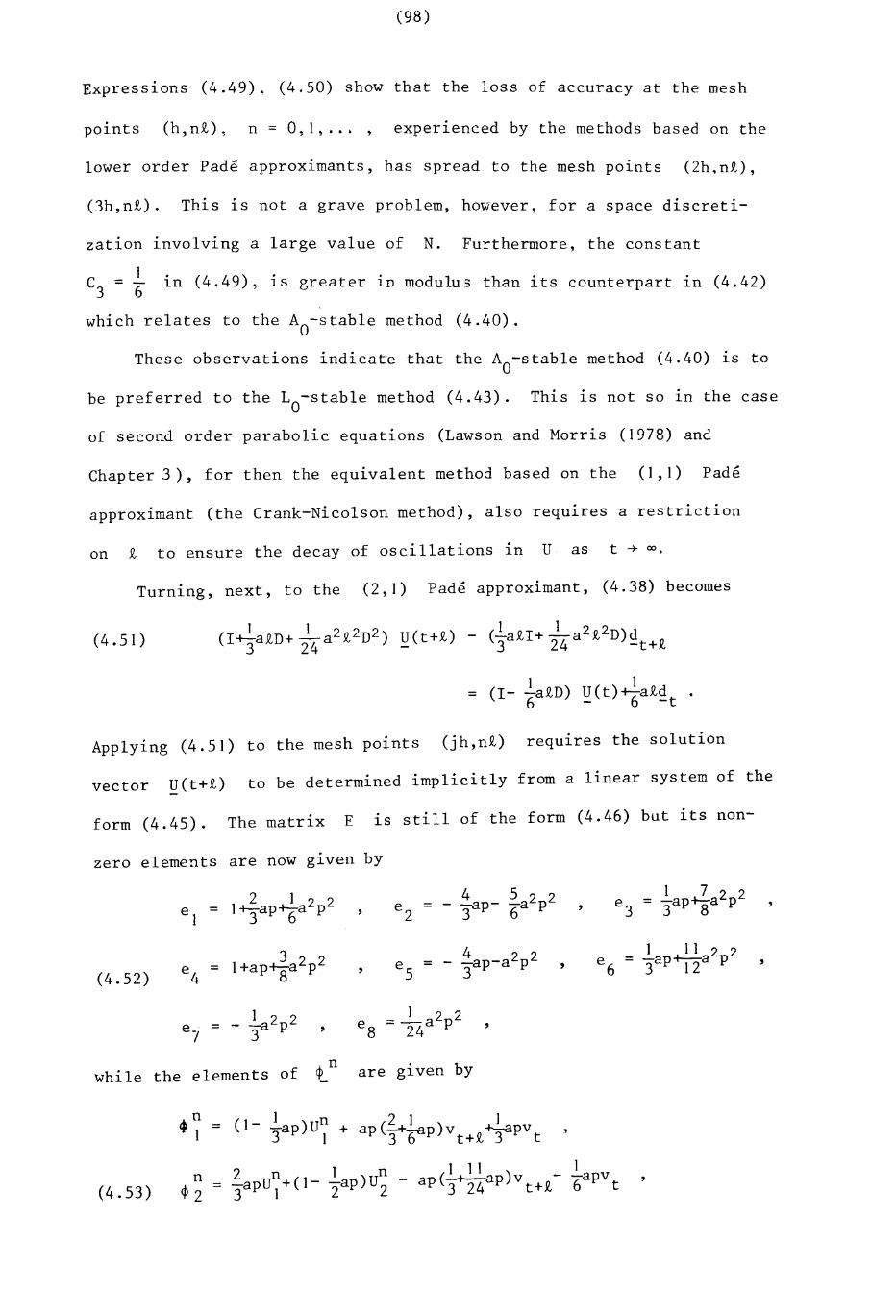
(98)
Expressions (4.49). (4.50) show that the loss of accuracy at the mesh
points (h,n£)~ n = O,l~ ... , experienced by the methods based on the
lower order Pade approximants, has spread to the mesh points (2h,n£),
(3h,n£). This is not a grave problem, however, for a space discreti-
zation involving a large value of N. Furthermore, the constant
1C3
= 6 in (4.49), is greater in modulus than its counterpart in (4.42)
which relates to the Ao-stable method (4.40).
These observations indicate that the Ao-stable method (4.40) is to
be preferred to the Lo-stable method (4.43). This is not so in the case
of second order parabolic equations (Lawson and Morris (1978) and
Chapter 3), for then the equivalent method based on the (1,1) Pade
approximant (the Crank-Nicolson method), also requlres a restriction
on £ to ensure the decay of oscillations in U as t ~ 00.
Turning, next, to the (2,1) Pade approximant, (4.38) becomes
(4.51)
Applying (4.51) to the mesh points (jh,n£) requlres the solution
vector U(t+£) to be determined implicitly from a linear system of the
f (4 45) The matr~ x E lS still of the form (4.46) but its non-orm .. ..L
zero elements are now glven by
I-tlap~a2p24 522 e
3= l-ap?a2p2
el
= e2
= - -ap- -a p ,3 6 3 6 3 8
1+ap~a2p2 iap-a2p21 11 2 2
e5
= e6
= -ap -+--:-a pe
4= , , 3 12
(4.52) 8 3
,-hnwhile the elements of ~
~~ = (1- ~p)U~ +
= _1_a2p 2e 8 24
are glven by
(4.53 )
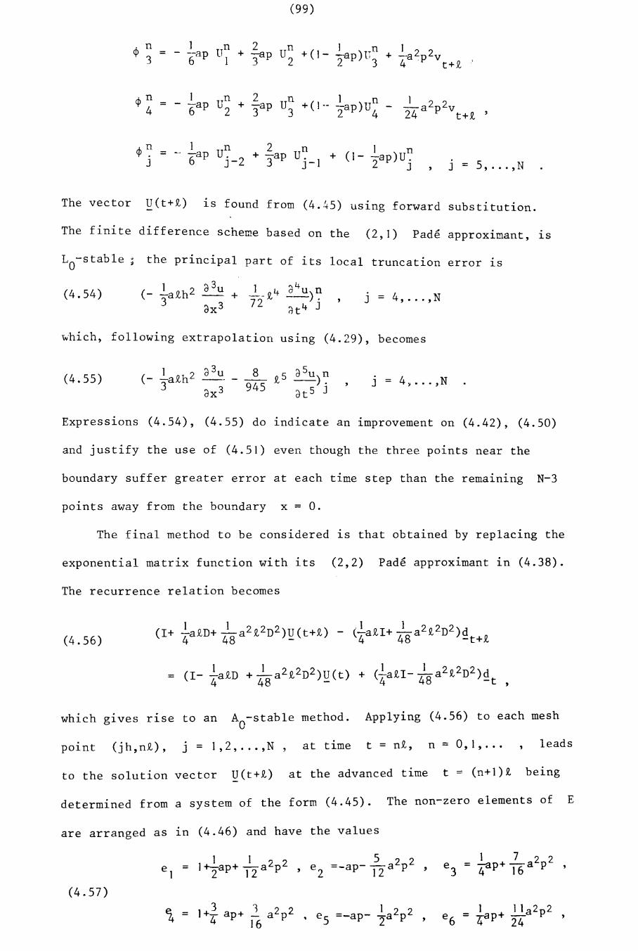
(99)
<p n ] Un 2 Un J n I= - --ap + -ap +(]- ~p)U + -:-a 2p 2v3 6 ] 3 2 2 3 4· t+£
<p n 1 Un 2 Un 1 n 1= - -ap + -ap + (J -. -ap)U -a2p2v4 6 2 3 3 2 4 24 t+£ ,
<p~ 1 n 2 n I n= _. -ap U. 2 + --ap U. 1 + (I - "2a p ) UjJ 6 J- 3 J- J = 5, ... , N
The vector ~(t+£) 1S found from (4.45) uS1ng forward substitution.
The finite difference scheme based on the (2,]) Pade approximant, 1S
J = 4, ... ,N
La-stable; the principal part of its local truncation error 1S
(_ la s.h 2 a3u + _]_£ 4 ~ 4u) r:3 dX 3 72 dt 4 J
(4.54)
which, following extrapolation uS1ng (4.29), becomes
(4.55) J = 4~ ... ,N
Expressions (4.54), (4.55) do indicate an improvement on (4.42), (4.50)
and justify the use of (4.5]) even though the three points near the
boundary suffer greater error at each time step than the remaining N-3
points away from the boundary x = a.
The final method to be considered 1S that obtained by replacing the
exponential matrix function with its (2,2) Pade approximant in (4.38).
The recurrence relation becomes
(4.56)
which g1ves r1se to an Ao-stable method. Applying (4.56) to each mesh
point (jh,n£), j = ],2, ..• ,N at time t = n£, n = a,I, ... leads
to the solution vector ~(t+£) at the advanced time t = (n+])£ being
determined from a system of the form (4.45). The non-zero elements of E
are arranged as 1n (4.46) and have the values
] ]=-ap- 2- a 2p 2 ~p+ 2- a 2p 2
= 1+-ap+ _a2p2 e 2e
3=e 1
, , 4 ]62 ]2 12
(4.57)
~3 ..l a 2p2 ~a2p2 1 1]a2p2= 1+4 ap+ "s =-ap- e 6 =• ~p+ 2416
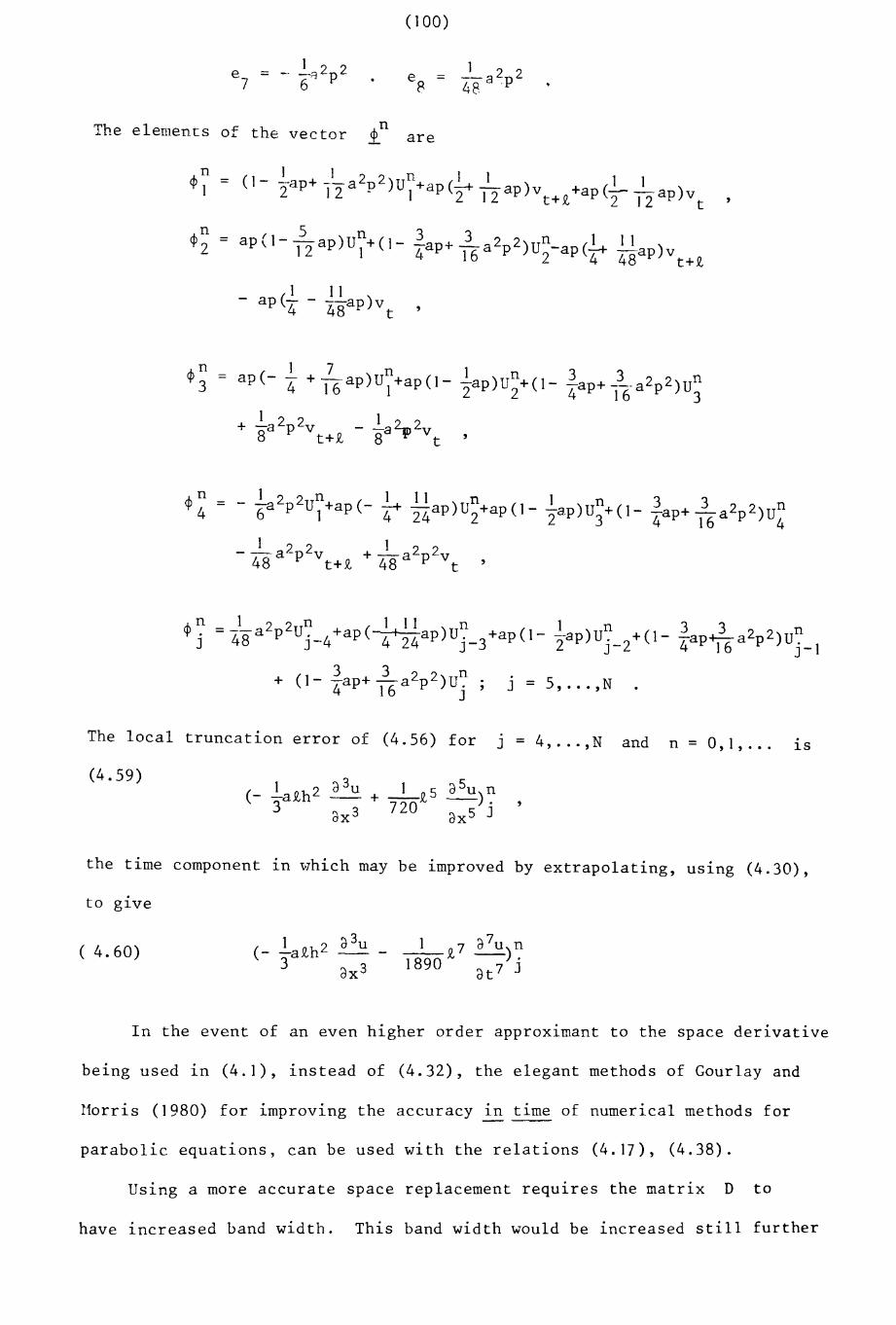
(100)
The elements of the vector
]e = -a 2p 2
8 48·
n1 are
= (1- 1 I 2 2) nIl 1 1Iap+ 12 a p U1+ap (-+2 -12 ap)v +ap (- -ap)v
t+ £, 2 12 t
¢n = (I 5 ) n 3 3 2 2 n 1 112 aP \ - 12ap U1+ ( 1- "4ap+ -16 a p )U
2- ap (""'+4 -ap)v
48 t+£'
1 11- ap (-4 - --ap)v
48 t
The local truncation error of (4.56) for J = 4, ... ,N and n = 0,1, ... 1S
(4.59)(__laoh2 a3u 1 5 a5u n
]V --+--£, -).3 ax 3 720 ax S J
the time component 1n which may be improved by extrapolating, uS1ng (4.30),
.to g1ve
( 4.60) 1 7 a7u n1890 £, -).
at7 J
In the event of an even higher order approximant to the space derivative
being used in (4.1), instead of (4.32), the elegant methods of Gourlay and
Horris (1980) for improving the accuracy 1n time of numerical methods for
parabolic equations, can be used with the relations (4.17), (4.38).
Using a more accurate space replacement requires the matrix D to
have increased band width. This band width would be increased still further
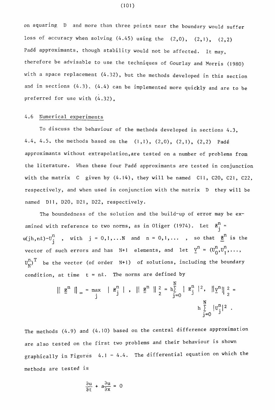
(101 )
on squar1ng D and more than three points near the boundary would suffer
loss of accuracy when solving (4.45) using the (2,0), (2,]), (2,2)
Pad€ approximants, though stability would not be affected. It may,
therefore be advisable to use the techniques of Gourlay and Morris (1980)
with a space replacement (4.32), but the methods developed in this section
and in sections (4.3), (4.4) can be implemented more quickly and are to be
preferred for use with (4.32),
4.6 Numerical experiments
To discuss the behaviour of the methods developed in sections 4.3,
4.4,4.5, the methods based on the (],l), (2,0), (2,1), (2,2) Pad€
approximants without extrapolation, are tested on a number of problems from
the literature. ~fuen these four Pade approximants are tested in conjunction
with the matrix C given by (4.14), they will be named Cll, C20, C21, C22,
respectively, and when used in conjunction with the matrix D they will be
named Dll, D20, D21, D22, respectively.
The boundedness of the solution and the build-up of error may be ex-
amined with reference to two norms, as 1n Oliger (1974). Let ~r: =J
u(j h, nt) -Ur: with J = O,I, ••. N and n = 0, 1, ... so that ~n 1S theJ
vector of such errors and has N+l elements, and letn n
= (U0' U1 ' ••• ,
II ~nI ,.J
max
Un)T be the vector (of order N+l) of solutions, including the boundaryN
condition, at time t = nt. The norms are defined by
NII 2 = hI I
2 j=ON
h I lur:12j=O J
The methods (4.9) and (4.10) based on the central difference approximation
are also tested on the first two problems and their behaviour 1S shown
4 4 The differential equation on which thegraphically in Figures 4.1 - ..
methods are tested is
dU dU+ a- = 0dt dX
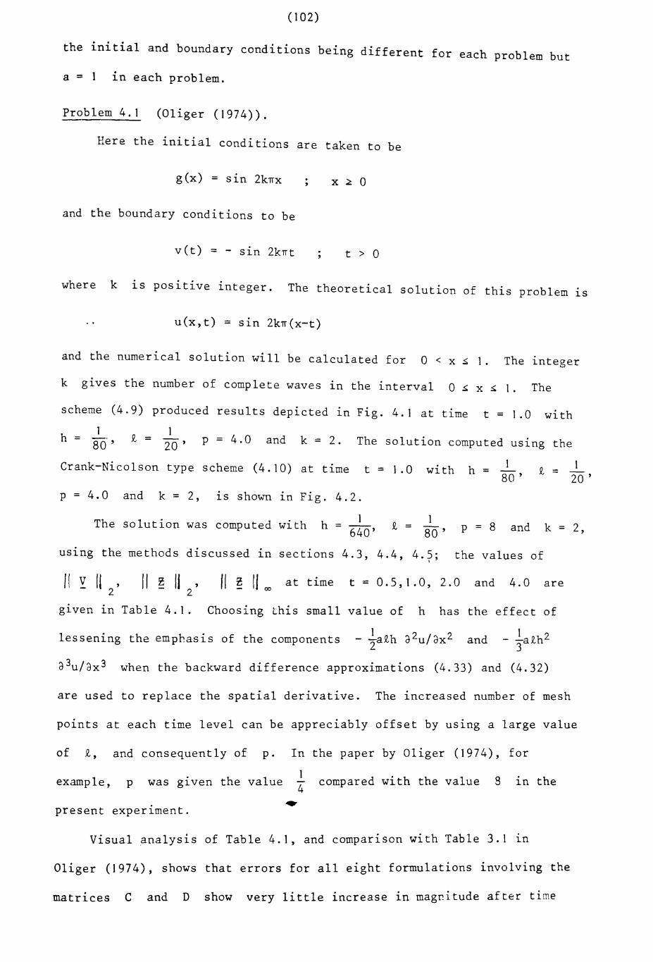
(l02)
the initial and boundary conditions being different for each problem but
a = 1 in each problem.
Problem 4.1 (Oliger (1974)).
Here the initial conditions are taken to be
g(x) = sin 2kTTX
and the boundary conditions to be
vet) = - sin 2kTTt
x ~ a
t > a
where k lS positive integer. The theoretical solution of this problem lS
u(x,t) = Sln 2kTT(X-t)
and the numerical solution will be calculated for 0 < x ~ 1. The integer
k gives the number of complete waves in the interval 0 / / 1"'" x"'" • The
scheme (4.9) produced results depicted in Fig. 4.1 at time t = 1.0 with
1h = _.80 '
1£ = 20' P = 4.0 and k = 2. The solution computed uSlng the
Crank-Nicolson type scheme (4.10) at time
p = 4.0 and k = 2, lS shown In Fig. 4.2.
t = 1.0 with 1h = 80'
1£ = 20'
The solution was computed with 1h = 640'
1£ =80 '
p = 8 and k = 2,
using the methods discussed in sections 4.3, 4.4, 4.5; the values ofI
II V II , II ~ II , II ~ II 00at time t = 0.5,1.0, 2.0 and 4.0 are- 2 - 2 -
.Table 4. 1. Choosing this small value of h has the effect ofglven In
lessening the emphasis of the components - .!.a£h a2u/ax2 and - l.a£h22 3
a3u/ax 3 when the backward difference approximations (4.33) and (4.32)
are used to replace the spatial derivative. The increased number of mesh
points at each time level can be appreciably offset by using a large value
of £, and consequently of p. In the paper by Oliger (1974), for
example, p was glven the value14
compared with the value 9 In the
present experiment.
Visual analysis of Table 4.1, and comparlson with Table 3.1 in
Oliger (1974), shows that errors for all eight formulations involving the
matrices C and D show very little increase in magr-itude after time
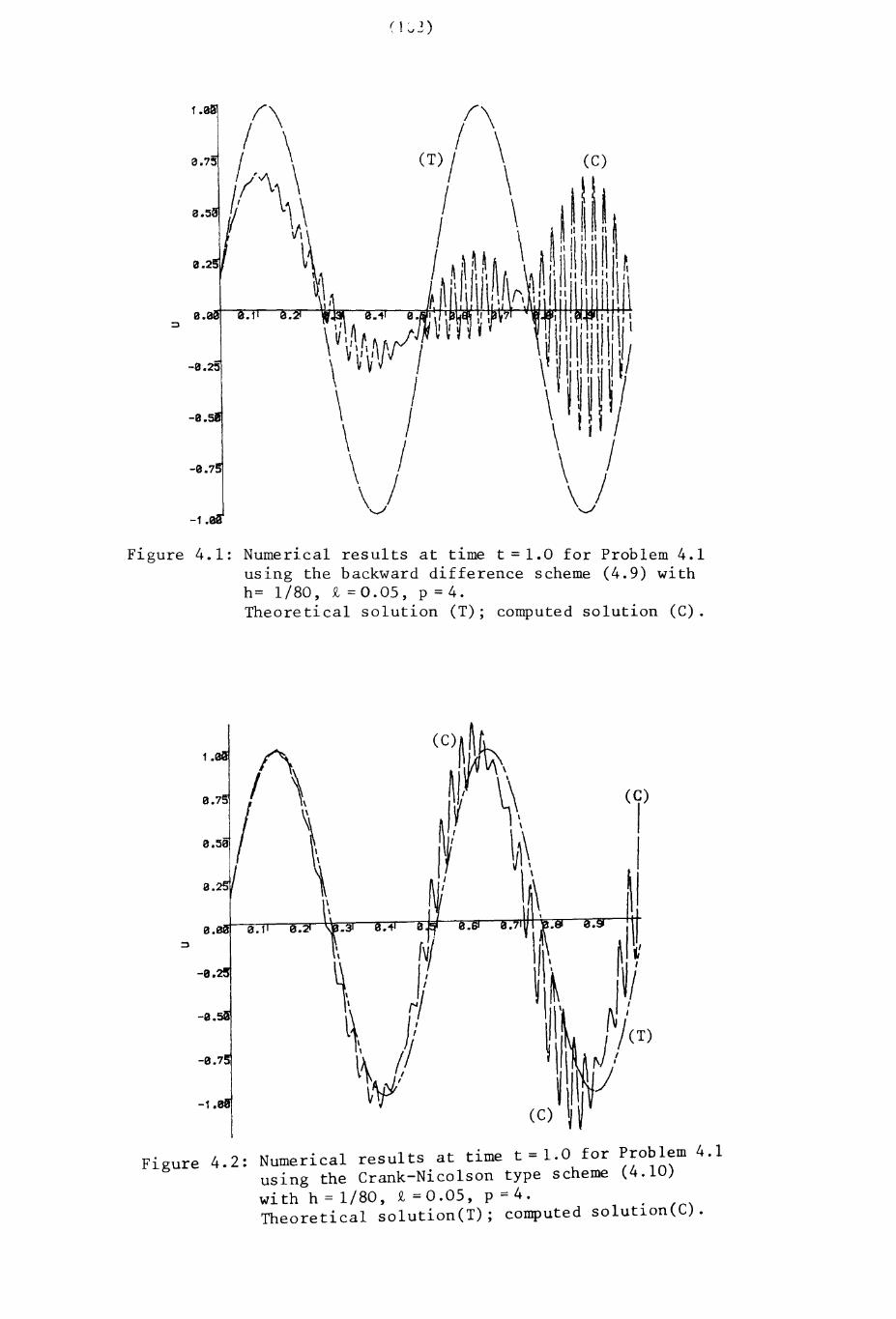
( i: J), v~
Figure 4.1: Numerical results at time t = 1.0 for Problem 4.1using the backward difference scheme (4.9) withh = 1 /80, £ = 0 . OS, p = 4.Theoretical solution (T); computed solution (C).
Figure 4.2: Numerical results at time t = 1.0 for Problem 4.1using the Crank-Nicolson type scheme (4.10)wi th h = 1/80, £ = 0 .05, p = 4.Theoretical solution(T); computed solution(C).
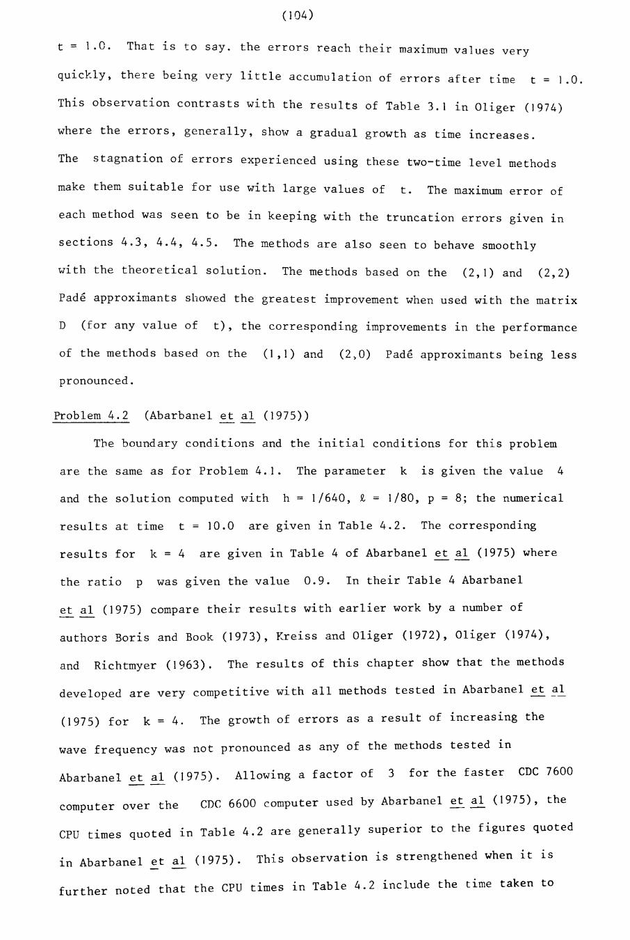
(104)
t = 1.0. That 1S to say. the errors reach their maX1mum values very
quickly, there being very little accumulation of errors after time t = 1.0.
This observation contrasts with the results of Table 3.1 in Oliger (1974)
where the errors, generally, show a gradual growth as time 1ncreases.
The stagnation of errors experienced uS1ng these two-time level methods
make them suitable for use with large values of t. The maximum error of
each method was seen to be in keeping with the truncation errors glven 1n
sections 4.3, 4.4, 4.5. The methods are also seen to behave smoothly
with the theoretical solution. The methods based on the (2,1) and (2,2)
Pade approximants showed the greatest improvement when used with the matrix
D (for any value of t), the corresponding improvements in the performance
of the methods based on the (1,1) and (2~0) Pade approximants being less
pronounced.
Problem 4.2 (Abarbanel et al (1975»)
The boundary conditions and the initial conditions for this problem
are the same as for Problem 4.1. The parameter k 1S given the value 4
and the solution computed with h = 1/640, £ = 1/80, P = 8; the numerical
results at time t = 10.0 are given in Table 4.2. The corresponding
results for k = 4 are given in Table 4 of Abarbanel et al (1975) where
the ratio p was glven the value 0.9. In their Table 4 Abarbanel
et al (1975) compare their results with earlier work by a number of--authors Boris and Book (1973), Kreiss and Oliger (1972), Oliger (1974),
and Richtmyer (1963). The results of this chapter show that the methods
developed are very competitive with all methods tested in Abarbanel et ~l
(I 975) for k = 4. The growth of errors as a result of increasing the
wave frequency was not pronounced as any of the methods tested in
Abarbanel et al (1975). Allowing a factor of 3 for the faster CDC 7600--
computer over the CDC 6600 computer used by Abarbanel et al (1975), the
CPU times quoted in Table 4.2 are generally superior to the figures quoted
(1975) Th1' s observation is strengthened when it 1Sin Abarbanel et al .
further noted that the CPU times in Table 4.2 include the time taken to

(\ (\I \ I \I \ I \I \ I \! \ I \ I
e. .1 0. -. rot . . ":i I
-e.20 \ I \ I \ I\ I \ I \ I
-e. \ I \ I \ I\ / \ / \ IV \) V
-1.
Figure 4.3: Numerical results at time t=lO.O for Problem 4.2using the backward difference scheme (4.9) withh = 1/80, £ = 0.05, p = 4.Theoretical solution (T); computed solution (C).
, (C)
,,~
-i
. 4 4' Numerical resul ts at time t = 10.0 forFl.gure .. Problem 4.2 using the Crank-Nicolson type
h (4 10) wi th h = 1/80, £ = 0" 05, p = 4"sc erne . . (C). 1 olutl.·on(T) "computed solutl.on .Theoretlca s ,
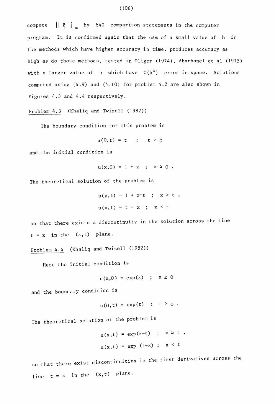
compute
(106)
II ~ II 00 by 640 comp ar i s on statements In the computer
program. It is confirmed again that the use of a small value of h ~n
the methods which have higher accuracy in time, produces accuracy as
high as do those methods, tested in Oliger (1974), Abarbanel et al (1975)
with a larger value of h which have 0(h4 ) error ~n space. Solutions
computed using (4.9) and (4.10) for problem 4.2 are also shown ~n
Figures 4.3 and 4.4 respectively.
Problem 4.3 (Khaliq and Twizell (1982))
The boundary condition for this problem ~s
u(O,t) = t
and the initial condition is
u(x,O) = 1 + x
t > °
x ~ ° ,The theoretical solution of the problem ~s
u(x,t) = + x-t
u(x,t) = t - x
x ~ t ,
x < t
so that there exists a discontinuity in the solution across the line
t = x ~n the (x,t) plane.
Problem 4.4 (Khaliq and Twizell (1982))
Here the initial condition ~s
u (x,O) = exp (x)
and the boundary condition is
u(O,t) = exp(t)
. 1 solut1'on of the problem ~sThe theoret~ca
u(x,t) = exp(x-t)
u(x,t) = exp (t-x)
x ~ 0
t > 0 .
x ~ t ,
x < t
., ~n the first derivatives across theso that there exist discontinu~t~es
line t = x in the (x,t) plane.
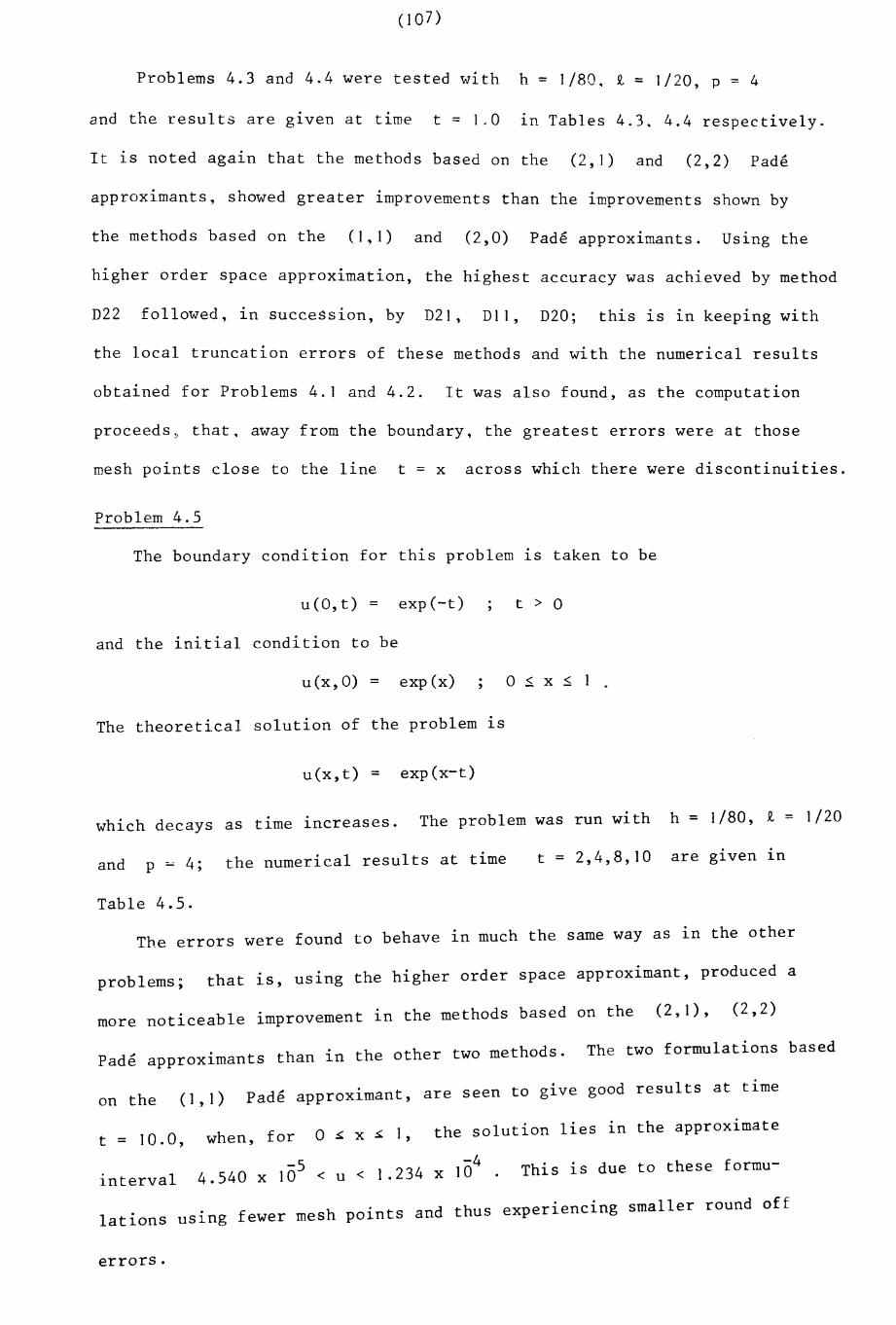
(10 7)
Problems 4.3 and 4.4 were tested with h = 1/80. t = 1/20, p = 4
and the results are given at time t = 1.0 in Tables 4.3. 4.4 respectively.
It is noted aga1n that the methods based on the (2,1) and (2,2) Pade
approximants, showed greater improvements than the improvements shown by
the methods based on the (1,1) and (2,0) Pade approximants. Using the
higher order space approximation, the highest accuracy was achieved by method
D22 followed, in succession, by D2I, DI I, D20; this is in keeping with
the local truncation errors of these methods and with the numerical results
obtained for Problems 4. I and 4.2. It was also found, as the computation
proceeds, that, away from the boundary, the greatest errors were at those
mesh points close to the line t = x across which there were discontinuities.
Problem 4.5
The boundary condition for this problem is taken to be
u(O,t) = exp(-t) t > °and the initial condition to be
u(x,O) = exp(x) ° ~ x ~
The theoretical solution of the problem 1S
u(x,t) = exp(x-t)
The problem was run with h = 1/80, t = 1/20which decays as time increases.
and p ~ 4; the numerical results at time
Table 4.5.
t = 2,4,8,10 are glven 1n
The errors were found to behave in much the same way as 1n the other
problems; that 1S, uS1ng the higher order space approximant, produced a
more noticeable improvement in the methods based on the (2,1), (2,2)
Pade approximants than in the other two methods. The two formulations based
on the ( I , I ). are seen to give good results at timePade approx1mant,
I the solution lies in the approximatet = 10.0, when, for ° ~ x ~ ,
-5 4 1-04 This is due to these formu-interval 4.540 x 10 < u < 1.23 x .
. d thus experiencing smaller round offlations using fewer mesh p01nts an
errors.
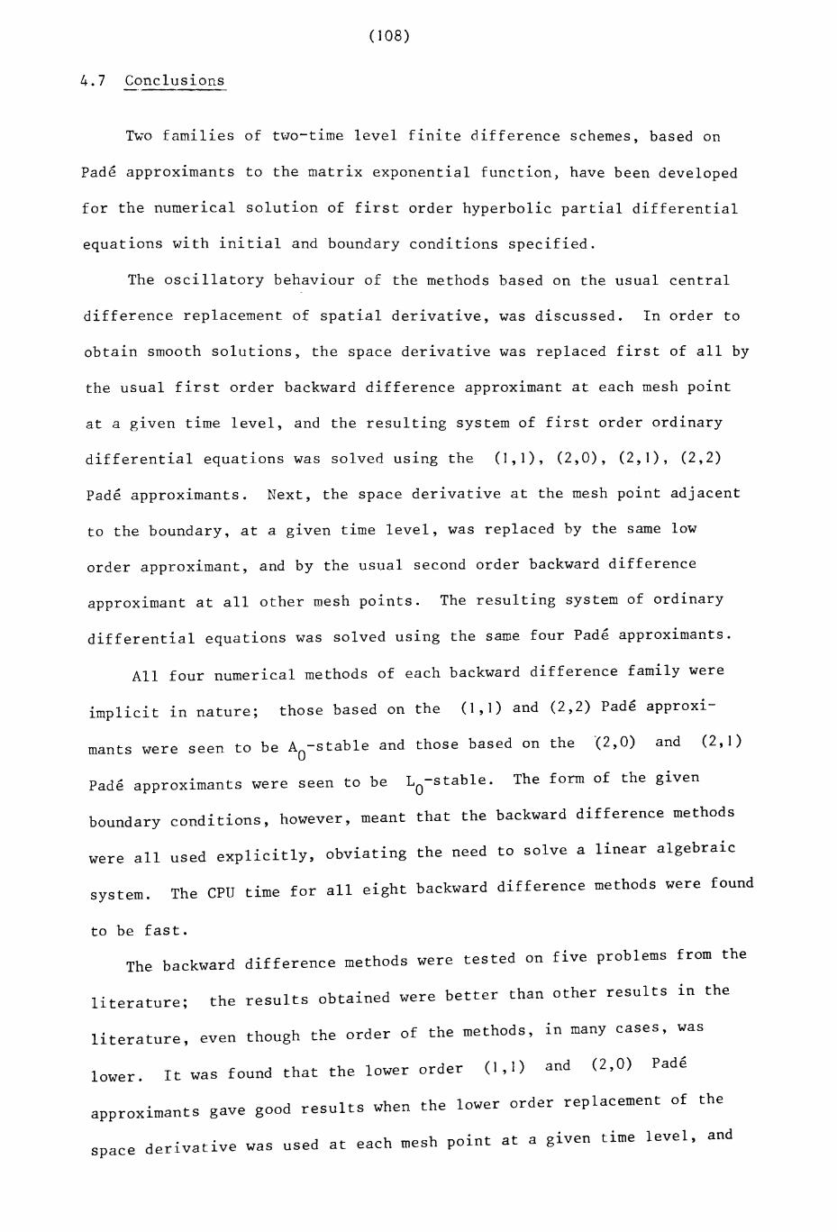
(108)
4.7 Conclusions
Two families of two-time level finite difference schemes, based on
Pad~ approximants to the matrix exponential function} have been developed
for the numerical solution of first order hyperbolic partial differential
equations with initial and boundary conditions specified.
The oscillatory behaviour of the methods based on the usual central
difference replacement of spatial derivative, was discussed. In order to
obtain smooth solutions, the space derivative was replaced first of all by
the usual first order backward difference approximant at each mesh point
at a given time level, and the resulting system of first order ordinary
differential equations was solved using the (1,1), (2,0), (2,1), (2,2)
Pad~ approximants. Next, the space derivative at the mesh point adjacent
to the boundary, at a given time level, was replaced by the same low
order approximant, and by the usual second order backward difference
approximant at all other mesh points. The resulting system of ordinary
differential equations was solved using the same four Pad~ approximants.
All four numerical methods of each backward difference family were
implicit in nature; those based on the (1,1) and (2,2) Pade approxi
mants were seen to be Ao-stable and those based on the {2,0) and (2,1)
Pade approximants were seen to be Lo-stable. The form of the g1ven
boundary conditions, however, meant that the backward difference methods
were all used explicitly, obviating the need to solve a linear algebraic
system. The CPU time for all eight backward difference methods were found
to be fast.
The backward difference methods were tested on five problems from the
literature; the results obtained were better than other results in the
literature, even though the order of the methods, in many cases, was
lower. It was found that the lower order (1,1) and (2,0) Pad~
approximants gave good results when the lower order replacement of the
space derivative was used at each mesh point at a given time level, and
(109)
that the higher order (2.1) and (2.2) Pade approximants gave their
best results when the higher order replacement of the space derivative
was used at interior mesh points. This implies that lower order
replacements in both space and time, or higher order replacements ln
both space and time. are most effective; this observation was also
made by Abarbanel et a1 (1975;p.351). For problems with decaying
solutions. the two backward difference formulations based on the (1,1)
Pade approximant give very good results due to the smaller number of
mesh points used, thus reducing round-off errors.
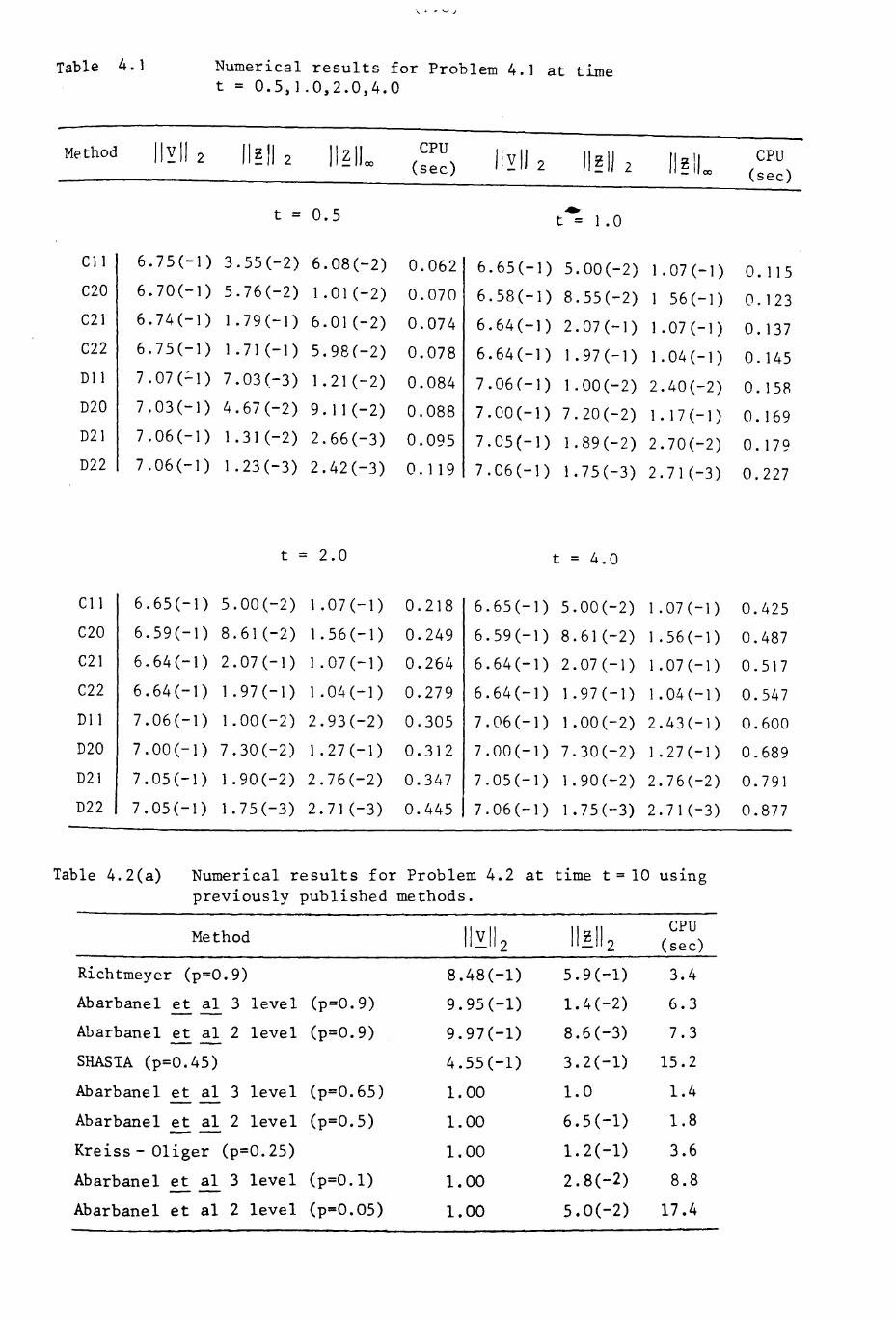
Table 4. 1 Numerical results for Problem 4.1 at timet = 0.5,1.0,2.0,4.0
Method 11~11 2 II~II 2 II ~ ILX)CPU
II ~ II 2 /I ~ II 2 II ~ 11eX)CPU
(sec) (sec)
t = 0.5 ~
t = 1.0
C11 6.75(-1) 3.55(-2) 6.08(-2) 0.062 6.65(-1) 5.00(-2) 1.07(-1) O. 115C20 6.70(-1) 5.76(-2) 1.01 (-2) 0.070 6.58(-1) 8.55(-2) 1 56(-1) 0.123C21 6.74(-1) 1.79(-1) 6.01(-2) 0.074 6.64(-]) 2.07(-1) ] .07 (-1 ) O. 137C22 6.75(-]) 1.71(-1) 5.98(-2) 0.078 6.64(-]) 1.97(-]) ] .04 (-1 ) O. ]45D11 7.07(':']) 7.03(-3) 1.2](-2) 0.084 7.06(-1) 1.00 (-2) 2.40(-2) O. 15RD20 7.03(-1) 4.67(-2) 9.11 (-2) 0.088 7.00(-]) 7.20(-2) 1.17(-1) O. 169D21 7.06(-1) 1.31(-2) 2.66(-3) 0.095 7.05(-]) 1.89(-2) 2.70(-2) O. 179D22 7.06(-1) 1.23(-3) 2.42(-3) O. 119 7.06(-]) 1.75(-3) 2.71(-3) 0.227
t = 2.0 t = 4.0
C11 6.65(-1) 5.00(-2) 1.07(-1) 0.218 6.65(-]) 5.00(-2) 1.07(-1) 0.425C20 6.59(-1) 8.61(-2) 1.56(-1) 0.249 6.59(-1) 8.61(-2) 1.56(-1) 0.487C21 6.64(-1) 2.07 (-1 ) 1.07(-1) 0.264 6.64(-1) 2.07 (-1 ) 1.07(-1) 0.517C22 6.64(-1) 1.97(-1) 1.04(-1) 0.279 6.64(-1) 1.97 (-1) 1.04 (-1 ) 0.547D11 7.06(-1) 1.00(-2) 2.93(-2) 0.305 7.06(-1) 1.00 (- 2) 2.43(-1) 0.600D20 7.00(-1) 7.30(-2) 1.27(-1) 0.312 7.00(-1) 7.30(-2) 1.27(-1) 0.689D21 7.05(-1) 1.90(-2) 2.76(-2) 0.347 7.05(-1) 1.90(-2) 2.76(-2) 0.791D22 7.05(-1) 1.75(-3) 2.71(-3) 0.445 7.06(-1) 1.75(-3) 2.71(-3) 0.877
Table 4.2(a) Numerical results for Problem 4.2 at time t = 10 usingpreviously published methods.
II vl1 2 11~112CPU
Method (sec)
Richtmeyer (p=0.9) 8.48(-1) 5.9(-1) 3.4
Abarbanel et al 3 level (p=0.9) 9.95(-1) 1.4(-2) 6.3--Abarbanel et al 2 level (p=0.9) 9.97(-1) 8.6(-3) 7.3--SHASTA (p=0.45) 4.55(-1) 3.2(-1) 15.2
Abarbanel et al 3 level (p=0.65) 1. 00 1.0 1.4--Abarbanel et a1 2 level (p=O. 5) 1.00 6.5(-1) 1.8--Kreiss - Oliger (p=0.25) 1.00 1.2(-1) 3.6
Abarbanel et al 3 level (p=O.l) 1.00 2.8(-2) 8.8--Abarbanel et al 2 level (p=0.05) 1.00 5.0(-2) 17.4
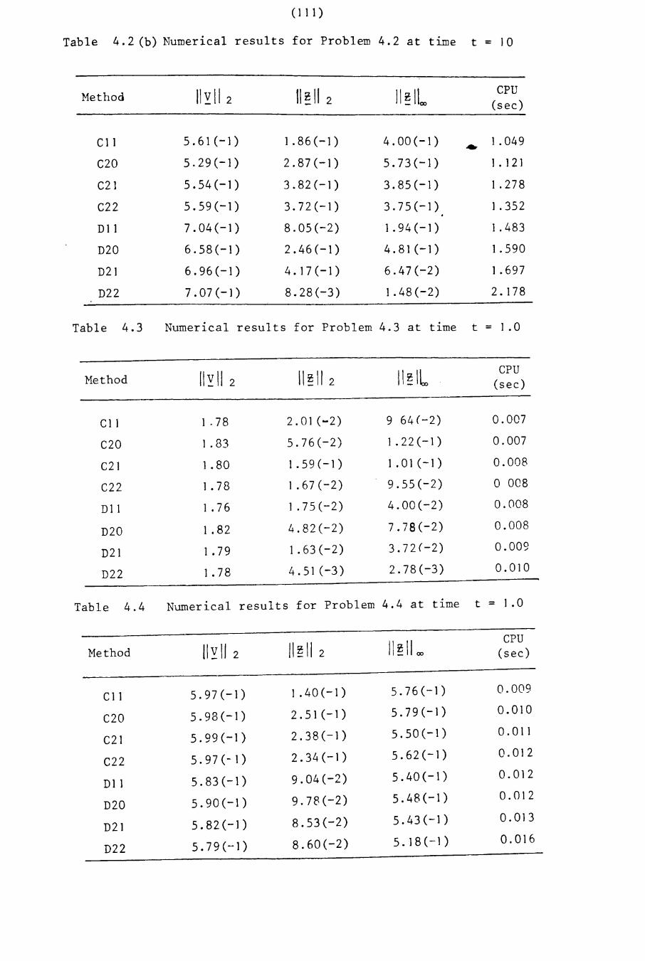
(111 )
Table 4.2 (b) Numerical results for Problem 4.2 at time t = 10
Method II ~ II 2 11 ~ II 2 II~ILCPU
(sec)
C11 5.61(-1) 1.86(-1) 4.00(-1) 1.049..C20 5.29(-1) 2.87(-1) 5.73(-1) 1. 121
C21 5.54(-1) 3.82(-1) 3.85(-1) 1.278
C22 5.59(-1) 3.72(-1) 3.75(-1) 1.352
D11 7.04(-1) 8.05(-2) 1.94(-1) 1.483
D20 6.58(-1) 2.46(-1) 4.81(-1) 1.590
D21 6.96(-1) 4.17(-1) 6.47(-2) 1.697
D22 7.07(-]) 8.28(-3) 1.48(-2) 2. 178
Table 4.3 Numerical results for Problem 4.3 at time t = 1. a
Method /I ~ II 2 11 ~ II 2 II~ILCPU
(sec)
C11 1.78 2.01(-2) 9 64(-2) 0.007
C20 1. 83 5.76(-2) 1.22(-1) 0.007
C21 1. 80 1.59(-1) 1.01(-1) 0.008
C22 1. 78 1.67(-2) 9.55(-2) a 008
D11 1. 76 1.75(-2) 4.00(-2) 0.008
D20 1. 82 4.82(-2) 7.78(-2) 0.008
D21 1. 79 1.63(-2) 3.72(-2) 0.009
D22 1. 78 4.51 (-3) 2.78(-3) 0.010
Table 4.4 Numerical results for Problem 4.4 at time t = 1. a
11~11 2 II~ II 2 II ~ 1100CPU
Method (sec)
C11 5.97(-1) 1.40(-1 ) 5.76(-1) 0.009
C20 5.98(-1) 2.51(-1) 5.79(-1) 0.010
C21 5.99(-]) 2.38(-1) 5.50(-1) 0.011
C22 5.97(-1) 2.34(-1) 5.62(-1) 0.012
D11 5.83(-1) 9.04(-2) 5.40(-1) 0.012
D20 5.90(-1) 9.78(-2) 5.48(-1) 0.012
D21 5.82(-1) 8.53(-2) 5.43(-1) 0.013
D22 5.79(--]) 8.60(-2) 5.18(-1) 0.016
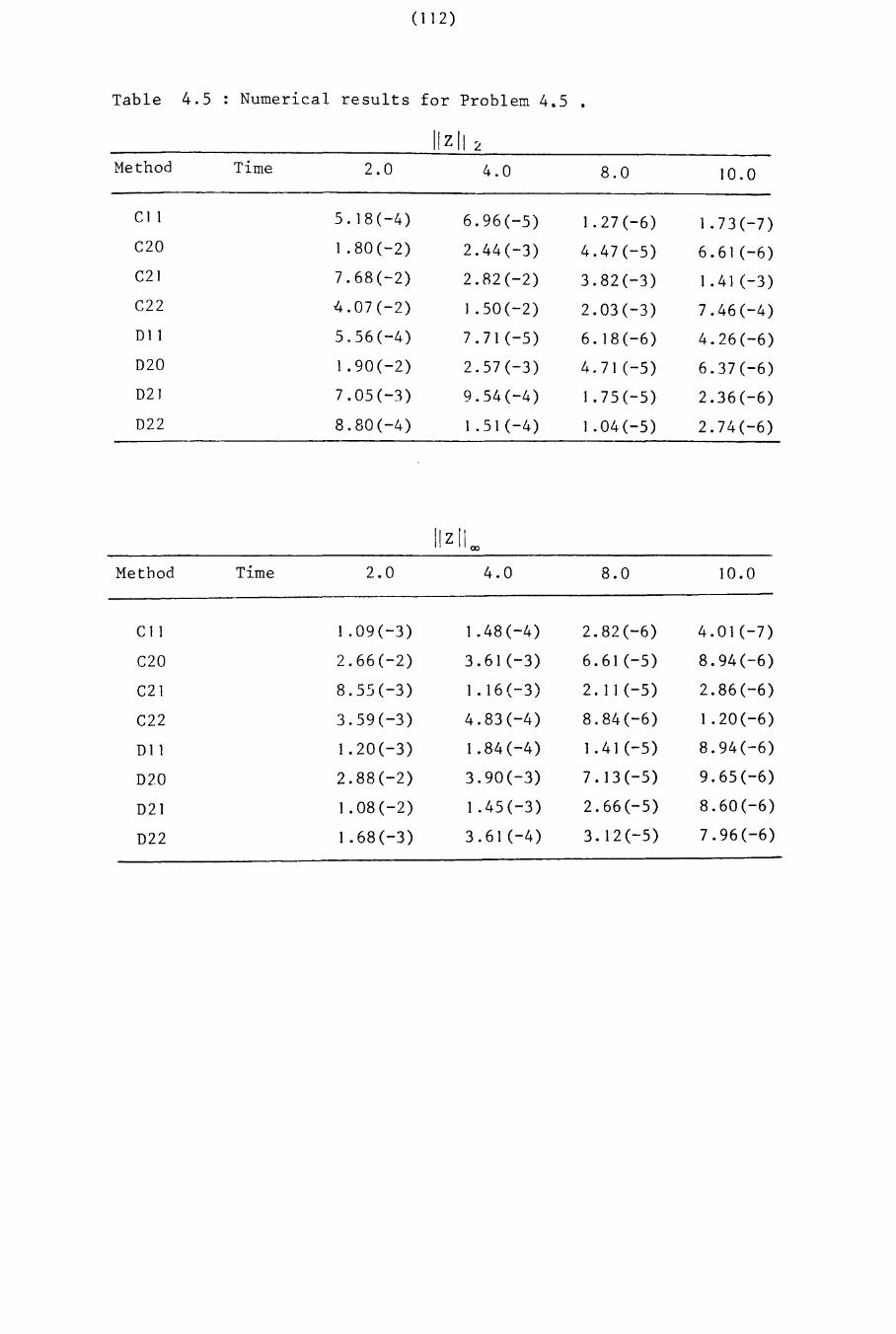
(I12)
Table 4.5 . Numerical results for Problem 4.5.
liz II L
Method Time 2.0 4.0 8.0 10.0
CI 1 5. 18(-4) 6.96(-5) 1.27(-6) 1.73(-7)C20 1.80(-2) 2.44(-3) 4.47(-5) 6.61 (-6)C21 7.68(-2) 2.82(-2) 3.82(-3) 1.4] (-3)C22 4.07(-2) 1.50(-2) 2.03(-3) 7.46(-4)D11 5.56(-4) 7.7](-5) 6.18(-6) 4.26(-6)
D20 1.90(-2) 2.57(-3) 4.71(-5) 6.37(-6)
D21 7.05(-3) 9.54(-4) 1. 75(-5) 2.36(-6)
D22 8.80(-4) 1.51 (-4) 1.04 (-5) 2.74(-6)
Method Time 2.0 4.0 8.0 10.0
C11 1.09(-3) 1.48 (-4) 2.82(-6) 4.01 (-7)
C20 2.66(-2) 3.61(-3) 6.61(-5) 8.94(-6)
C2] 8.55(-3) 1.16(-3) 2.11(-5) 2.86(-6)
C22 3.59(-3) 4.83(-4) 8.84(-6) 1.20(-6)
D1] 1.20(-3) 1.84(-4) 1.41(-5) 8.94(-6)
D2.0 2.88(-2) 3.90(-3) 7.13(-5) 9.65(-6)
D21 1.08(-2) 1.45(-3) 2.66(-5) 8.60(-6)
D22 1.68(-3) 3.61(-4) 3.12(-5) 7.96(-6)
(I13 )
CHAPTER 5
SECOND ORDER PERIODICINITIAL VALUE PROBLEMS
5.1 Introduction
Periodic initial value 'problems of the form yll = f(x,y) ar1se 1n the
theory of orbital mechanics, and in recent years there has been considerable
interest in the numerical solution of such problems.
Generally speaking, second order initial value problems can be divided
into two distinct classes: (a) problems for which the solution period is
known in advance; (b) problems for which this period is unknown initially.
Numerov's methods applied to type (a) always stays on the orbit, whereas the
..Stormer-Cowell methods with step number greater than two spiral inwards. In
the terminology of Stiefel and Bettis (1969), the former method 1S orbitally
stable, the latter orbitally unstable. Modified numerical methods have been
proposed by Gautschi (1969), Stiefel and Bettis (1969) and Jain et al (1979),
which can be used to compute the solution for problems of type (a). For the
numerical solution of problems of type (b), it is desirable that the method
should be P-stable. Lambert and Watson (1976) have shown that certain linear
multistep methods of arbitrary stepnumber possess a periodicity property when the
product of steplength and angular frequency lies within the interval of period-
icity and these authors developed symmetry conditions under which a linear multi-
step method possesses a non-vanishing interval of periodicity. However, Lambert
and Watson have shown a P-stable linear multistep method cannot have order of
accuracy greater than 2. Jain et al (1979) have derived higher order methods
and claim that they are P-stable. It is noted that their concept of P-
stability 1S considerably weaker than that given by Lambert and Watson (1976).
Higher order P-stable methods are also proposed by Cash (1981) and Chawla (1981)
whose methods need three function evaluation at each step. Cash (1981) has
tested his fourth and sixth order P-stable methods on numerical examples and

(114)
achieved higher accuracy than Lambert and Watson (1976), by uSlng the ana
lytical solution to compute the solution with steplength h at y(h).
However, for practical problems, it is usually necessary to use a starting
procedure.
In section 5.2 of this chapter, a recurrence relation is developed
which yields two-step multiderivative methods, employing Pade approximants
to the exponential functions. The definition of P-stability given by
Lambert and Watson (1976, p.199), is adapted. The methods are analysed ln
section 5.3. The interval of periodicity, principal part of local truncation
errors and non-zero coefficients for the algorithms yielded by the first six
teen entries of the Pade Table (Appendix I) are given in
Appendix III. The two-step multiderivative methods are given ln Appendix IV.
Fourth and sixth order methods based on the (2,2) and (3,3) Pade approximants
are tested for comparison purposes on the problems discussed by Cash (1981),
in section 5.4. The methods are analysed in PECE mode and tested on numerical
examples discussed by Jain et al (1979) and Shampine and Gordon (1973) in
section 5.5. Finally, conclusions are drawn in section 5.6.
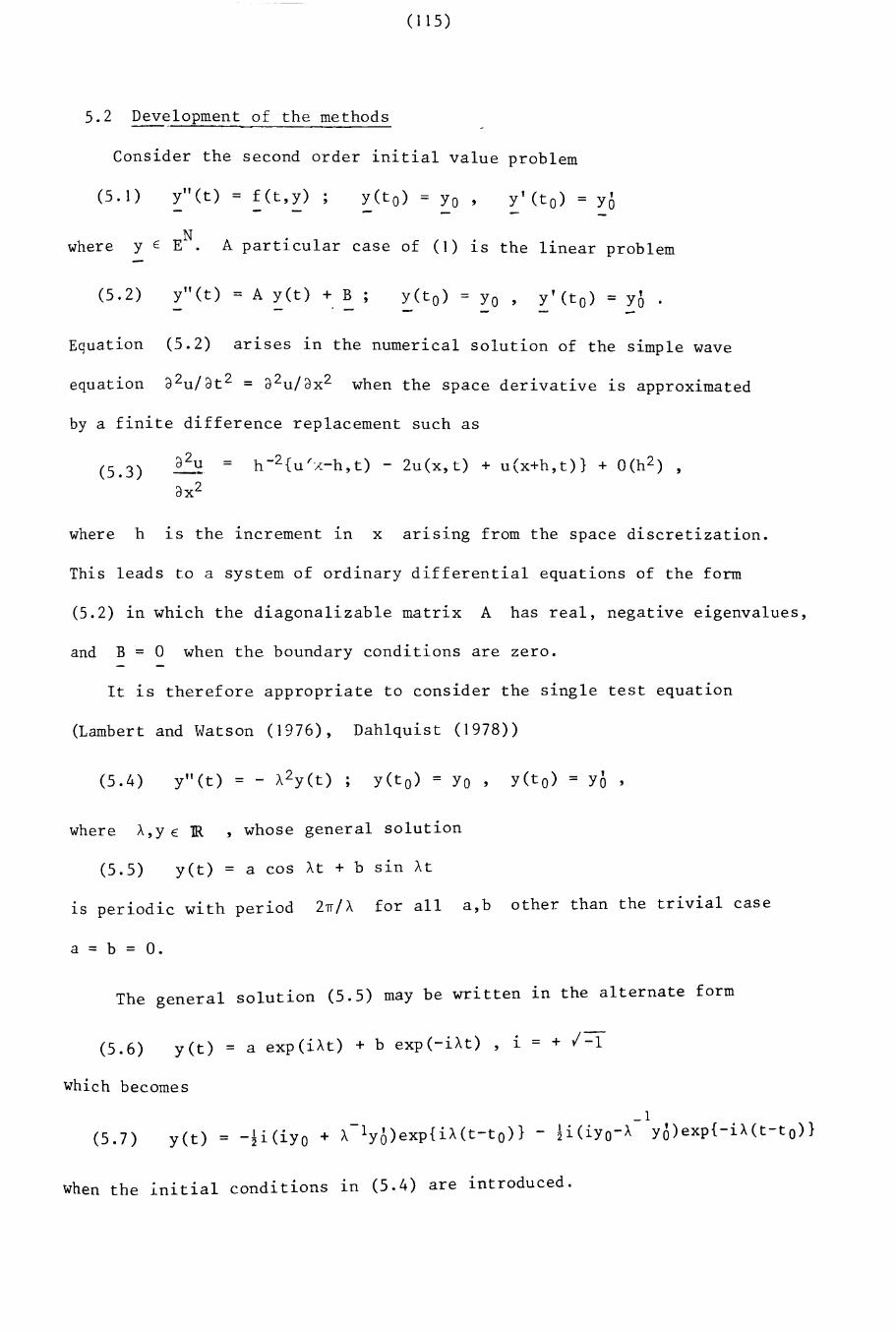
( 115)
5.2 Dev~lopment of the methods
Consider the second order initial value problem
(5. 1) y"(t) = f(t,y) ; y(to) = YO ,
where y E EN. A particular case of (1) ~s the linear problem
(5.2) y"(t) = A yet) + B ;
Equation (5.2) arises ~n the numerical solution of the simple wave
equation 32u/3t 2 = 32u/3x2 when the space derivative is approximated
by a finite difference replacement such as
(5.3) =
where h is the increment ~n x ar~slng from the space discretization.
This leads to a system of ordinary differential equations of the form
(5.2) in which the diagonalizable matrix A has real, negative eigenvalues,
and B = 0 when the boundary conditions are zero.
It is therefore appropriate to consider the single test equation
(Lambert and Watson (1976), Dahlquist (1978))
(5.4) y"(t) = - A. 2y(t)
where A.,y E 1R , whose general solution
(5.5) yet) = a cos A.t + b s~n A.t
1S periodic with period 2n/A. for all a,b other than the trivial case
a = b = O.
The general solution (5.5) may be written ~n the alternate form
(5.6) yet) = a exp(iA.t) + b exp(-iA.t) , i = + /-1
which becomes
(5.7)
_1y(t) = -~i(iyO + A.- 1yo)exp{iA.(t-to)} - ~i(iYO-A YO)exp{-iA(t-tO)}
When the initial conditions in (5.4) are introduced.
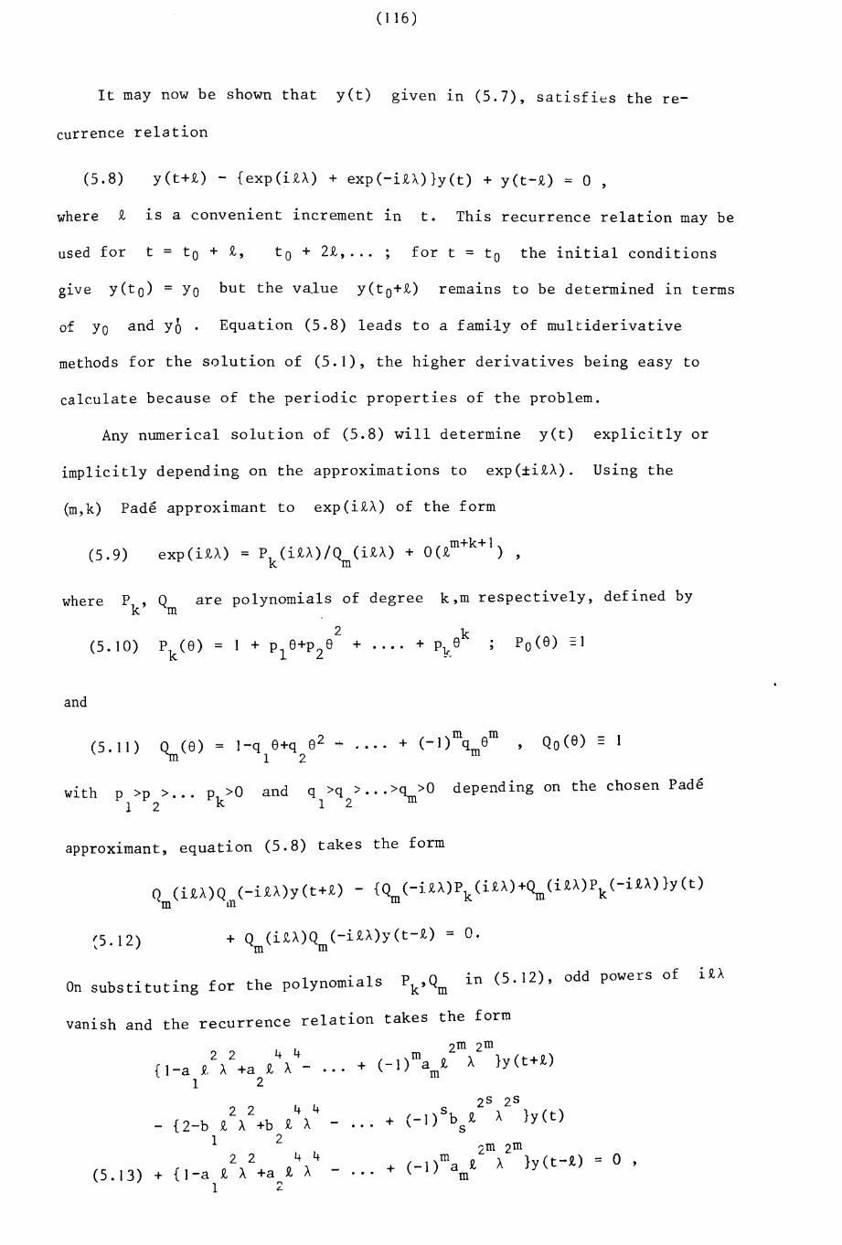
( 116)
It may now be shown that yet) glven ln (5.7)~ satisfies the re-
currence relation
(5.8) y(t+t) - {exp(itA) + exp(-itA)}y(t) + y(t-£) = 0 ,
where t is a convenient increment in t. This recurrence relation may be
used for t = to + t, to+2t, ... for t = to the initial conditions
gIve y(to) = YO but the value y(to+t) remains to be determined in terms
of YO and Yo. Equation (5.8) leads to a family of multiderivative
methods for the solution of (5.1), the higher derivatives being easy to
calculate because of the periodic properties of the problem.
Any numerical solution of (5.8) will determine yet) explicitly or
implicitly depending on the approximations to exp(±itA). Using the
(m,k) Pade approximant to exp(itA) of the form
(5.9) exp(itA) = Pk(i£A)/Q (i£A) + O(£m+k+l) ,m
where P Q are polynomials of degree k,m respectively, defined byk ' m
(5.10)k
+ •.•. + Pk8
and
QO(8) = 1(5.11 ) 2 .... (_I)m 8mo (8) = 1-q 8+q 8 .. . .. + q ,1n 12 m
'th >0 d q >q > ••• >q >0 depending on the chosen PadeWI p >p >... Pk an -m
1 2 1 2
approximant, equation (5.8) takes the form
Q (itA)Q (-itA)y(t+t) - {Q (-itA)P (itA)+Q (i£A)Pk(-itA)}y(t)m III m k m
~5.12)+ Q (itA)Q (-itA)y(t-t) = O.
m m
, f h 1 ol'als Pk,Qm In (5.12), odd powers ofOn substitutlng or t e po yn m
vanish and the recurrence relation takes the form
2 2 4 4 2m
2m
{Ir-a 9. A +a t A - ... + (-l)mamt A }y(t+£)1 2
2 2 4 4- {2-b t A +b t A - ... +
1 22 2 4 4
(5.13) + {l-a t A +a t A - ... +1 2
2 s 2 s(_l)sb t A }y(t)
s2m 2m
(_l)ma t A }y(t-t) = 0 ,m
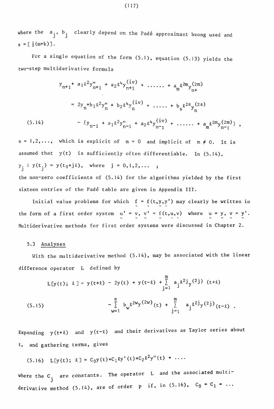
(117)
where the a j, b j clearly depend on the Pade approximant beong used and
s = [ ! (m+k) ] .
For a single equation of the form (5.1), equation (5.13) yields the
two-step multiderivative formula
+ •••••• + a £2m (zm)m Yn+
(5. 14)
= 2y +b £2y" + b £4v(iv)n 1 n 2..1 n +
n = 1,2, ... , which ~s explicit of m = 0 and implicit of m ~ o. It ~s
assumed that yet) ~s sufficiently often differentiable. In (5.14),
y. = y(t.) = y(tO+j£), where j = 0,1,2, ...J J
the non-zero coefficients of (5.14) for the algorithms yielded by the first
sixteen entries of the Pade table are g~ven in Appendix III.
Initial value problems for which f = f(t,y,y') may clearly be written ~n
the form of a first order system u' = v, v' = f(t,u,v) where u = y, v = y'.
Multiderivative methods for first order systems were discussed ~n Chapter 2.
5.3 Analyses
With the multiderivative method (5.14), may be associated with the linear
difference operator L defined by
m
L [y ( t ); £ ] = Y( t +£) - 2y (t ) + y ( t - £) +j ~ 1 a j £2j Y(2j) ( t +£)
(5. 15)s
- Lw=l
and y(t_O) and their derivatives as Taylor ser~es aboutExpanding y(t+£) N
t, and gathering terms, g~ves
where the C.J
are constants. L and the associated multiThe operator
derivative method (5.14), are of order p if, in (5.16), Co = C1 = ...
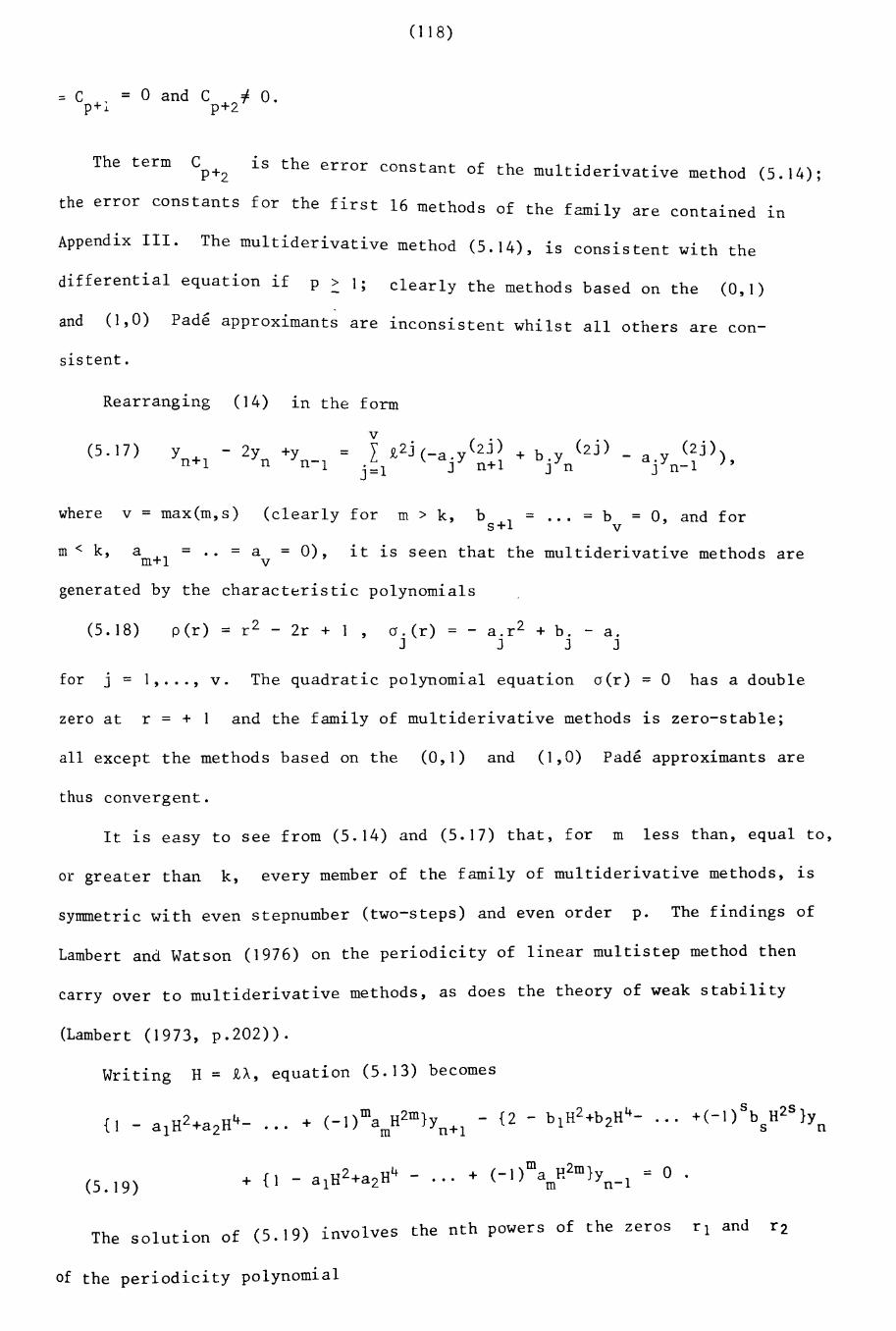
(118)
::: C +' = ° and C =f 0.P J. p+2
The term C 1S thP+2 e error constant of the multiderivative method (5.14);
the error constants for the first 16 methods of the family are contained 1n
Appendix III. The multiderivative method (5.14), is consistent with the
differential equation if p _> I,' 1c early the methods based on the (0,1)
and (1,0) Pade approximant~ are inconsistent whilst all others are con-
sistent.
Rearranging (14) 1n the form
(5. 17) y - 2y +yn+1 n n-1 = a.y (2 j ) )
J n-1 '
where v = max(m,s) (clearly for m > k, bS+1 = .•. = b
v= 0, and for
m < k, a =m-r I
= a = 0)v ' it is seen that the multiderivative methods are
generated by the characteristic polynomials
(5.18) per) = r 2 - 2r + I , a.(r) = - a.r2 + b. - a.J J J J
for J = I, ... , v. The quadratic polynomial equation a(r) = ° has a double
zero at r = + and the family of multiderivative methods is zero-stable;
all except the methods based on the (0,1) and (1,0) Pade approximants are
thus convergent.
It is easy to see from (5.14) and (5.17) that, for m less than, equal to,
or greater than k, every member of the family of multiderivative methods, 1S
symmetric with even stepnumber (two-steps) and even order p. The findings of
Lambert and Watson (1976) on the periodicity of linear multistep method then
carryover to multiderivative methods, as does the theory of weak stability
(Lambert (1973, p.202)).
Writing H = £A, equation (5.13) becomes
(5. 19)
The solution of (5.19) involves the nth powers of the zeros rl and r2
of the periodicity polynomial
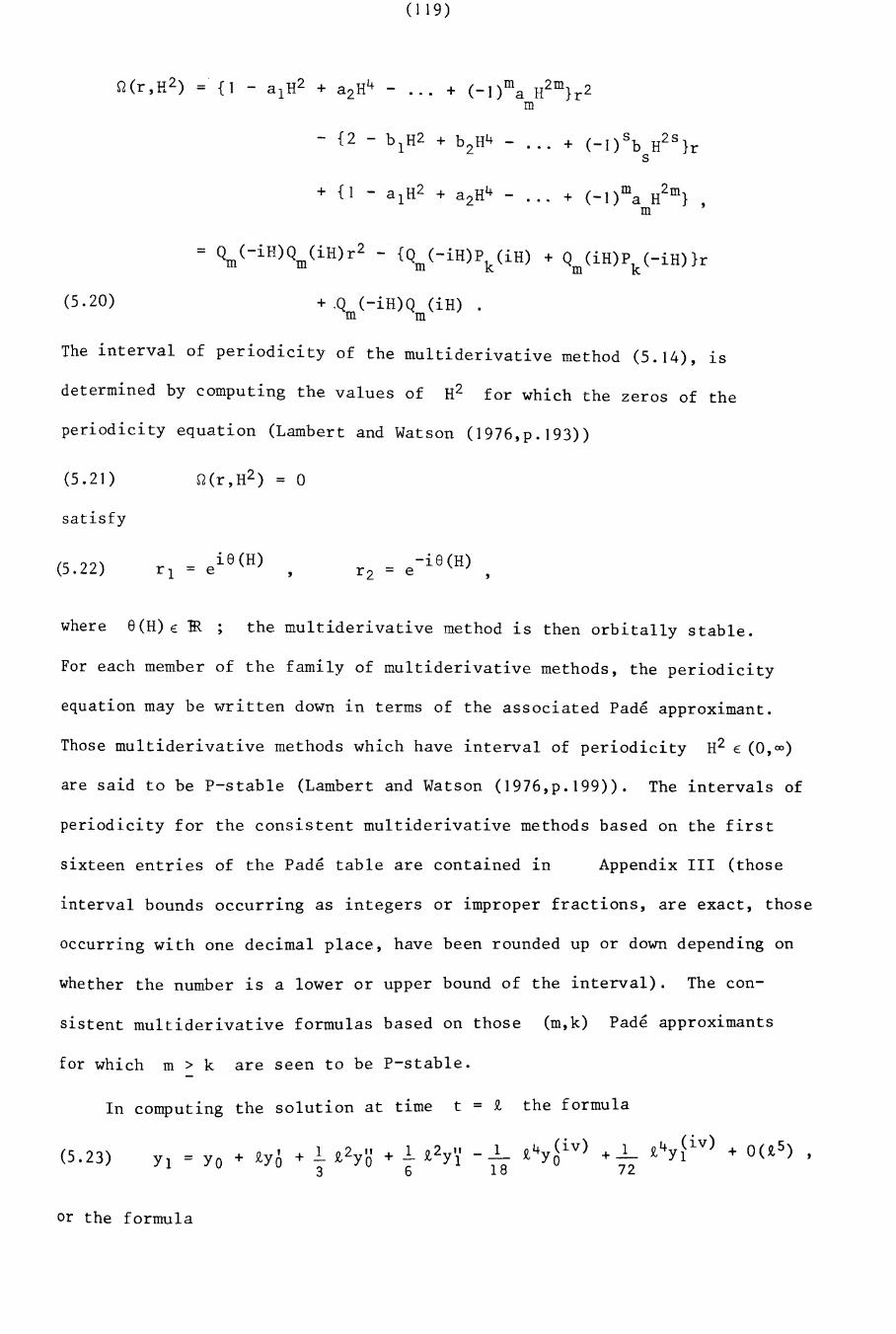
(119 )
( m 2m 2... + -I) a H Lrill
(5.20)
+ {I - a1H2 + a2H4 - ... + (-l)ma H2m}m
= Qm(-iH)Qm(iH)r2 - {Qm(-iH)Pk(iH) + Qm(iH)Pk(-iH)}r
+.Q (-iH)Q (iH) .m m
The interval of periodicity of the multiderivative method (5.14), lS
determined by computing the values of H2 for which the zeros of the
periodicity equation (Lambert and Watson (1976,p.193»
(5.21 )
satisfy
(5.22) = e i 8 (H)r1-i8(H)
r2 = e ,
where 8 (H) E JR the multiderivative method is then orbitally stable.
For each member of the family of multiderivative methods, the periodicity
equation may be written down in terms of the associated Pade approximant.
Those multiderivative methods which have interval of periodicity H2 E (0,00)
are said to be P-stable (Lambert and Watson (1976,p.199». The intervals of
periodicity for the consistent multiderivative methods based on the first
sixteen entries of the Pade table are contained in Appendix III (those
(5.23)
interval bounds occurring as integers or improper fractions, are exact, those
occurring with one decimal place, have been rounded up or down depending on
whether the number is a lower or upper bound of the interval). The con-
sistent multiderivative formulas based on those (m,k) Pade approximants
for which m > k are seen to be P-stable.
In computing the solution at time t = £ the formula
= Yo + £Ya' + 1... £ 2y '0' + 1- £2y '1 - 1 £4y ~ i v) + _1_ £4yfi v) + 0 (£ 5) ,Yl 3 6 18 72
or the formula

(120)
Yl = YO + £yO + 1.. £2yO + 1 £2Y'1 1 £4 (iv) __7_ £4y(iv)- - - YO3 6 45 360 1
(5.24 ) + 1 £6 (vi) 11 £6 (vi) + 0(£7)-- YO - Yl108 2160 ,
(Twizell (1981)) may be used in solving problems which are known to have
outward-spiralling theoretical solutl·ons. 0 h' ,t erwIse, Taylor s series may be
used to gIve y, to the necessary accuracy.
To investigate absolute stability, the family of multiderivative methods
are applied to the single test equation (5.4). -Writing h = _£2 A2
(Lambert (1973,p.258)), the stability polynomial for each of the methods
from equation (5.13) takes the form
-1T(r,h) = + ... + a ~)(r2+1)
m
(5.25 )
~d the interval of absolute stability (Dahlquist (1978,pp.133-134)), are
found by solving the equation
(5.26)
In each case.
-n(r,h) = °
Methods based on the (m,k) Pade approximants for m ~ k are found
to be A-stable, whilst methods based on the (m,k) Pade approximants for
m < k have finite interval of absolute stability hE[ -a,OJ. The value
of a is in fact the same as for the interval of periodicity H2 E (O,a).
The analogy between P-stability and A-stability for two-step symmetric
multistep methods, is thus obvious for the family of multiderivative methods
developed in section (5.2), see also Dahlquist (1963, 1978), Lambert and
Watson (1976), Chawla (1981) and Hairer (1979).
5.4 Numerical examples
The family of multiderivative methods developed In section 5.2, were
tested on two problems well known in the literature. Numerical results for
methods based on the (2,2) and (3,3) Pade approximants, are presented

(121)
1n this section.
Problem 5. 1
This is the almost periodic problem introduced by Stiefel and Bettis
(1969) and considered by Lambert and Watson (1976) and Cash (198]). It is
given by
Z" = - z + O. 00] ite z(O):::] , z'(O) = 0.9995 1, z C.
The theoretical solution satisfies
u(t) = cos t + a .0005 t sin t , u E JR
v( t ) = sin t - 0.0005 t cos t , V E JR
z(t) = u I t ) + LvCt)
and represents the motion of the point z(t) on a perturbation of a
circular orbit. The distance of this point from the centre of the orbit
at time t is given by
I I
y(t) = [u2(t) + V2 ( t ) J 2 = [] + (0.0005t)2J2
so that the point spirals slowly outwards as time Increases.
Following Lambert and W~tson (]976), the differential equation is written
In the form of the real linear system
u" = -u + O. 00 1 cos t ; u (0) = 1 , u' (0) = 0(5.27 )
v" = -v + O. 00] sin t ; v(O) = 0, v ' (0) = 0.9995
f rom which the higher derivatives, for use with the multiderivative methods
developed in section 5.2 are easily determined.
The numerical solutions U(t) , V(t) of the real system (5.27), were com-
puted at t=40n for £ = n/4, n/5, n/6, n/9, n/]2, using the multi-
derivative methods based on the (2,2), (3,3) Pade approximants. The corre-
sponding computed values Z(t), f(t) of z(t), y(t) were then computed
using
Z(t) = U(t) + iV(t) ,1
I' (t ) = [ U2 (t ) + V2 (t ) ] 2 •
The error moduli in the computed values Z(t), f(t) g1ven by
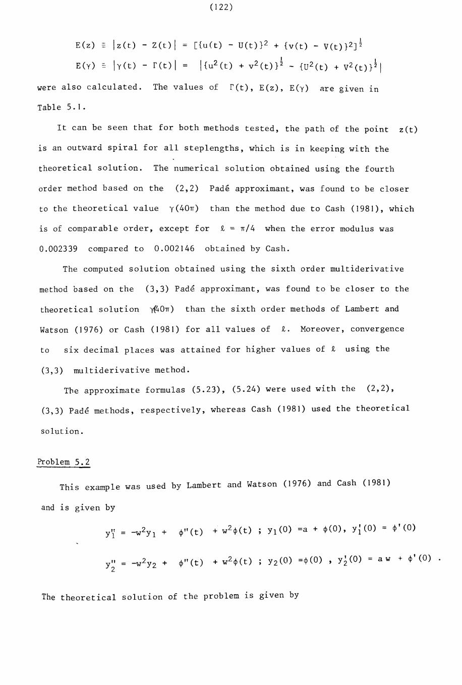
(122)
I= [{u(t) - U(t)}2 + {vet) - V(t)}2J2
1 I
l{u2(t) + V2 (t ) }2 - {U2(t) + V2(t)}21
Z (t ) I
ret) I =
E(z) - Iz(t)
E(Y) - h(t)
were also calculated. The values of ret), E(z), E(y) are glven In
Table 5. 1.
It can be seen that for both methods tested, the path of the point z(t)
is an outward spiral for all steplengths, which is in keeping with the
theoretical solution. The numerical solution obtained using the fourth
order method based on the (2,2) Pade approximant, was found to be closer
to the theoretical value y(40rr) than the method due to Cash (1981), which
lS of comparable order, except for £ = rr/4 when the error modulus was
0.002339 compared to 0.002146 obtained by Cash.
The computed solution obtained using the sixth order multiderivative
method based on the (3,3) Pade approximant, was found to be closer to the
theoretical solution ~40rr) than the sixth order methods of Lambert and
Watson (1976) or Cash (1981) for all values of t. Moreover, convergence
to six decimal places was attained for higher values of t using the
(3,3) multiderivative method.
The approximate formulas (5.23), (5.24) were used with the (2,2),
(3,3) Pade methods, respectively, whereas Cash (1981) used the theoretical
solution.
Problem 5.2
This example was used by Lambert and Watson (1976) and Cash (1981)
and is given by
Y'l = -W2Yl + </>"(t) + w2</>(t) ; Yl (0) =a + cj>(0), yi (0) = </>' (0)
" 2 h." (t ) + w2A-. (t )Y = -w Y2 + '¥ '¥
2Y2(O) =</>(0) , y~(O) = aw + cj>' (0) .
The theoretical solution of the problem lS glven by
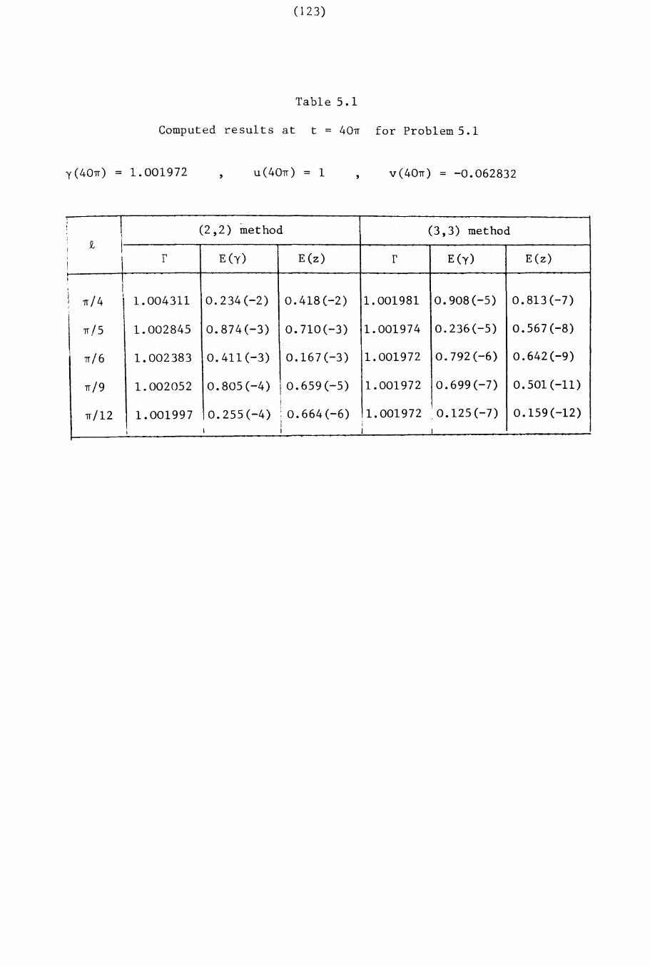
(123)
Table 5.1
Computed results at t = 40n for Problem 5.1
y(40n) = 1.001972 , u(40n) = 1 , v(40n) = -0.062832
,\ (2,2) method (3,3) method
:
II 9-,
\r E (y) E(z) r E(y) E(z )
!J I,i n/4
I
1.004311 0.234(-2) 0.418(-2) 0.908(-5) 0.813(-7)I 1.001981I
n/5 1.002845 0.874(-3) 0.710(-3) 1.001974 0.236(-5) 0.567(-8)
J
n/6 1.002383 0.411(-3) 0.167(-3) 1.001972 0.792(-6) 0.642(-9)
n/9 1.002052 0.805(-4) 0.659(-5) 1.001972 0.699(-7) 0.501(-11)
n/12 1.001997 0.255(-4) 0.664(-6) 1. 001972 :0.125(-7) 0.159(-12)i
I I I I
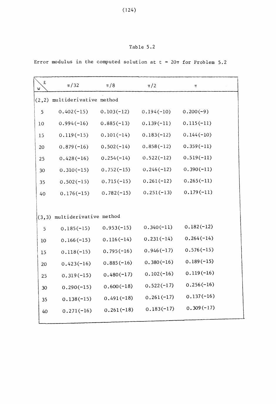
(124)
Table 5.2
Error modulus ~n the computed solution at t = 20~ for Problem 5.2
rx ~/32 ~/8 ~/2 rr
\(2:2) mu1tiderivative method
0.402(-15) 0.103(-12) 0.194(-10) 0.200(-9)I
\10 0.994(-16) 0.885(-13) 0.139(-11) 0.115(-11)
15 0.119(-15) 0.101(-14) 0.183(-12) 0.144(-10)
20 0.879(-16) 0.502(-14) 0.858(-12) 0.359(-11)
25 0.428(-16) 0.254(-14) 0.522(-12) 0.519(-11)
30 0.310(-15) 0.752 (-15) 0.246(-12) 0.390(-11)
35 0.502(-15) o. 715 (-15) 0.261(-12) 0.265(-11)
40 0.176(-15) 0.782(-15) 0.251(-13) 0.179(-11)
(3,3) mu1tiderivative method
5 0.185(-15) 0.953(-15) 0.340 (-11) 0.182(-12)
10 0.166(-15) 0.116(-14) 0.231(-14) 0.264(-14)
15 0.118(-15) 0.795(-16) 0.946(-17) 0.576(-15)
20 0.423(-16) 0.885(-16) 0.380(-16) 0.189(-15)
25 0.319(-15) 0.480 (-17) 0.102(-16) 0.119(-16)
30 0.290(-15) 0.600(-18) 0.522(-17) 0.256(-16)
35 0.138(-15) 0.491(-18) 0.261 (-17) 0.137(-16)
40 0.271(-16) 0.261(-18) 0.183(-17) 0.309 (-17)
( 125)
Y1(t ) = a cos wt + ¢ (t )
Y1(t ) = a sin wt + ¢ (t )
and, following Lambert and Watson (1976) and Cash (1981), ~()'t' t 1S taken to
be-O.OSt
e The parameter a was given the value zero , corresponding to
the case when high frequency oscillations are not present in the theoretical
solution. The results at t = 20TI for w = 5(5)40 and £ = TI/32, /TI 8,TI/2,TI
are g1ven in Table 5.2.
Comparing Table 5.2 with Table 2 in Cash (1981), it 1S seen that,
except in the isolated case w = 5,£ =TI/8, the fourth order multiderivative
method tested in the present paper gives better results than the fourth
order method of Cash; the sixth order method tested in the present paper
always gives superior results to the sixth order method in Cash (1981)
when applied to Problem 5.2
As with Problem5.1,formulas (5.23), (5.24) were used to compute y(£).
5.5 Use in PECE mode
In common with texts and other papers, the convention of associating an
asterisk with a predictor formula will be adopted. Using the general (O,k*)method as predictor and the general (m,k) method as corrector, the combinationin PECE mode will be denoted by (O,k*);(m,k).
It is not necessary to choose a predictor formula for which k* = max(m,k)
and the existing theory relating to the order of the local truncation error
of linear multistep methods used 1n PECE mode carr1es over to multiderivative
methods used in PECE mode. In particular, if the order of the predictor 1S
at least the order of the corrector, then the error constant of the pre-
dictor-corrector combination is that of the corrector alone. In addition,
if the predictor and the corrector have the same order p ,then Milne's
device
(5.28 ) C [ ( c ) (P) / * - C ]p+2 Yn+l- Yn+1J [Cp+2 p+2
may be used to estimate the error constant of the predictor-corrector com-
bination in PECE mode (provided *C 2 i: C -).p+ p-iZIn (5.26), the superscripts
(F) and (C)
(126)
refer to the predictor and corrector, respectively.
The periodicity polynomial ~ (H2)PECE r, of the (O,k*); (m,k) com-
bination in PECE mode may be shown to take the form
(5.29)
where s* = [!k*] .
m+ I (-I)ja.H2j
j= 1 J
s*I (-I)wb*H2W]r + 1
w=l w
The interval of periodicity of the (0 k*) (k) ., , . ; m, pr ed i.c t orr-cor r e c tor
combinat~on is determined by computing the v tlues of H for which the zeros
of the periodicity equation
satisfy (5.22).
It was found that the (0,2); (1,2) combination, with error constant1
C4 = 36 and periodicity interval H2 E (0,9), has the smallest modulus
error constant and the greatest interval of periodicity of the second order
combinations.
Of the fourth order combinations, it was found that the (0,4); (2,2)1
combination, for which C6 = 360 and H2 E (0,15.89), is to be preferred to
any fourth order combination when solving non-linear problems, because it
requires no more than the second derivative of f(t,¥). For linear problems-7
the (0,4); (1,3) combination which has C6 = 2880 and H2E (0,4.88), may be
used with small values of £ if higher accuracy is needed.
For non-linear problems of the form (5.1), the maximum steplength which
may be used at any time t of the calculation, has the value H*/A(t)
where H2 E (0,H*2) 1S the periodicity interval of the predictor-corrector
combination being used, and A2(t) 1S the largest modulus real part of the
eigenvalues of the Jacobian af/ay at time- - t
Th (0 4) (2 2) method was tested on the following problem which wase , ; ,
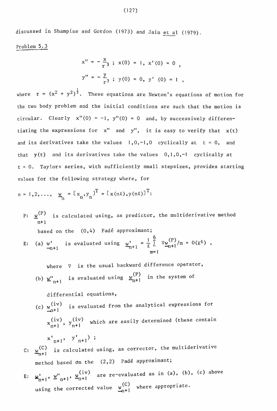
(127)
discussed in Shampine and Gordon (1973) and Jain et al (1979).
Problem 5.3
x" xx(O)= ;3 = 1, x' (0) = ° ,
y" =y
yeO) 0, y' (0) 1r 3 = = ,I
where r = (x2 + y2)2. These equations are Newton's equations of motion for
the two body problem and the initial conditions are such that the motion 1S
circular. Clearly x"(O) = -1, y"(O) = 0 and, by successively differen-
tiating the expressions for x" and y", it is easy to verify that x(t)
and its derivatives take the values 1,0,-1,0 cyclically at t = 0, and
that yet) and its derivatives take the values 0,1,0,-1 cyclically at
t = 0. Taylors series, with sufficiently small stepsizes, provides starting
values for the following strategy where, for
n = 1,2, ... , wn
1S calculated uS1ng, as predictor, the multiderivative methodP:
E:
w(P)
n+l
based on the (0,4) Pade approximant;
1 6(a) w' is evaluated using w' = n L
-n+l -n+l N
m=l
where V 1S the usual backward difference operator,
(b) w"- n+1
1S evaluated using(P)
w11+1in the system of
differential equations,
(c) w(iv) is evaluated from the analytical express10ns for-11+ 1
(iv) (iv) which are easily determined (these containxn+ 1 ' Yn+1
c: (C)w-n+l
is calculated uS1ng, as corrector, the multiderivative
method based dn the (2,2) Pade approximant;
are re-evaluated as in (a), (b), (c) aboveE: , (iv)w" w.w.n+1, - n+1' -n+1
the Cor r e c t ed valueuS1ng(C)
w~+1
where appropriate.
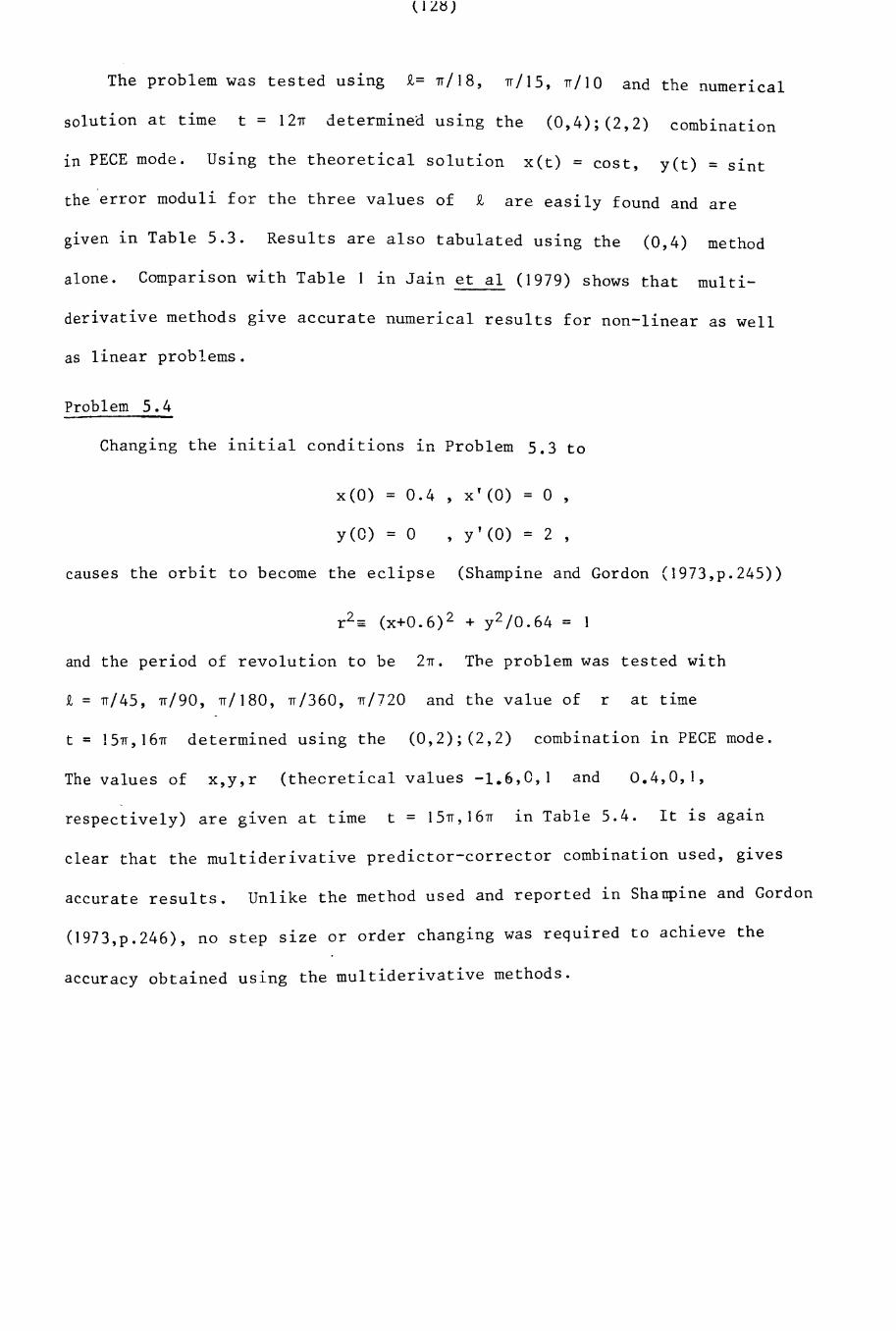
(Il~)
Problem 5.4
Changing the initial conditions In Problem 5.3 to
x(O) = 0.4 , x'(O) = 0 ,
y (0) = 0 , y' (0) = 2
causes the orbit to become the eclipse (Shampine and Gordon (1973,p.245))
r 2 ; (x+0.6)2 + y2/0.64 = 1
and the period of revolution to be 2n. The problem was tested with
~ = rr/45, n/90, n/180, n/360, n/720 and the value of r at time
t = 15n,16n determined using the (0,2);(2,2) combination in PECE mode.
The values of x,y,r (thecretical values -1.6,0,1 and 0.4,0,1,
respectively) are given at time t = 15n,16n in Table 5.4. It is agaln
clear that the multiderivative predictor-corrector combination used, gives
accurate results. Unlike the method used and reported in Sharrpine and Gordon
(1973,p.246), no step size or order changing was required to achieve the
accuracy obtained using the multiderivative methods.
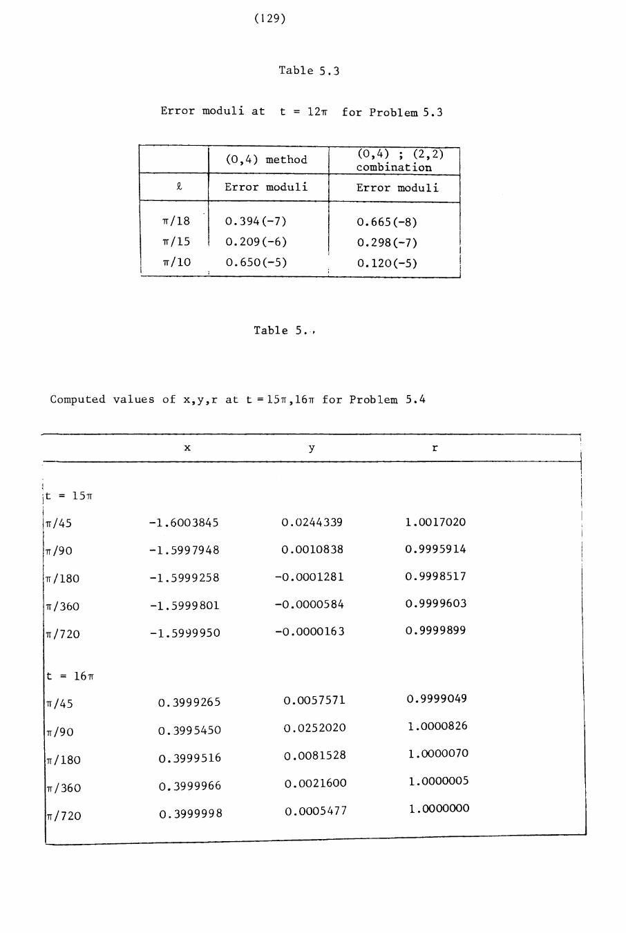
(129)
Table 5.3
Error moduli at t = 12TI for Problem 5.3
0.120( 5)650( 5)/
(0,4) method (0,4) . (2,2),combination
s. Error moduli Error moduli
TI/18 0.394(-7) 0.665(-8)
TI/15 0.209(-6) 0.298(-7) II I
TI 10 o. - - I
Table 5.r
Computed values of x, y, r at t =15TI ,16if for Prob 1em 5.4
x y r
't = 15TII
if/45 -1.6003845 0.0244339 1.0017020
if/90 -1.5997948 0.0010838 0.9995914
if/180 -1.5999258 -0.0001281 0.9998517
if/360 -1.5999801 -0.0000584 0.9999603
if/720 -1.5999950 -0.0000163 0.9999899
t = 16TI
if/45 0.3999265 0.0057571 0.9999049
TI/90 0.3995450 0.0252020 1.0000826
if/180 0.3999516 0.0081528 1.0000070
if / 360 0.3999966 0.0021600 1.0000005
if/720 0.3999998 0.0005477 1.0000000
(130)
5.6 Conclusions
A family of two-step multiderivative methods, based on Pade approxi
mants to the exponential function, has been developed for periodic initial
value problems of second order ordinary d'ifferential equations. The method
based on the (0,2) Pade approximant is seen to be the usual explicit
method. The method based on the (1,1) Pade approximant, is found to be
the formula, found to be unconditionally stable by Richtmyer and Morton
(1967,p.263) in connection with the solution of second order hyperbolic
equations, and discussed for second order ordinary differential equations
by Dahlquist (1978). However, the topic of Dahlquists paper was un
conditional stability, not P-stability.
The methods based on the (m,k) Pade approximants, for m ~ k, are
found to be P-stable, while the methods for m < k are seen to have finite
interval of periodicity. Following Dahlquist (1963, 1978), Lambert and
Watson (1976) and Hairer (1979), it is concluded that for two-step multi
derivative methods, the analogy between P-stability and A-stability is
obvious. Numerical experiments have confirmed that the two-step multi
derivative methods developed in this chapter glve higher accuracy than the
fourth and sixth order two-step Runge-Kutta type methods developed by
Cash (1981). For non-linear problems, where higher derivatives cannot be
calculated with ease, predictor-corrector combinations can be used. The
application of the methods for fourth order parabolic partial differential
equations in one and two space dimensions, will be discussed in Chapter 6.
(131 )
CIIAPTER 6
FOURTH ORDER PARABOLIC EQUATIONS
6.1 Introduction
The fourth order parabolic partial differential equation ~n one
space variable given by
(6. 1) a2u a4u-+jJ-=Oat2 ax 4
., jJ > 0,0 < x < X,t > 0
arlses ln the study of the transverse vl·bratl·ons of auniform flexible
beam (see, for example, Gorman (1975». The term jJ is the ratio of
the flexural rigidity of the beam to its mass per unit length.
The initial conditions associated with (6.1) are of the form
(6.2) u (x , 0) = gO(x) . 0 .s; x .s; X,
(6.3) au (x , 0) = g 1(x ) 0 :;;; x .s; Xat
and the boundary conditions are glven by
(6.4) u(O,t) = fO u(X,t) = f
1 t > 0
(6.5) a 2u (0, t ) = Po a2u(X,t) = PI t > 0,ax 2 ax 2
In (6.2), (6.3) the functions gO(x), gl(x) are continuous and r n (6.4),
(6.5) the terms f O' f 1, PO' PI are real constants.
To compute the solution of (6.1) with (6.2), (6.3), (6.4), (6.5),
explicit and implicit finite difference schemes have been proposed by
Albrecht (1957), Collatz (1951), Conte (1957), Conte and Royster (1956),
and Crandall (1954). Evans (1965) derived finite difference methods by
first writing (6.1) as two simultaneous second order parabolic partial
differential equations (see also Dufort and Frankel (1953), and Richtmyer
(1957». Explicit and implicit finite difference methods based on the
semi-explicit method of Lees (1961) and the high order method of Douglas
(1956) for second order parabolic equations, have been formulated for the
numerical solution of (6.1) with (6.2), (6.3) by Fairweather and Gourlay
(132)
(1967).
The explicit method of Collatz (1951) frequently needs a large
number of time steps to compute the solution in view of the stability
restriction on the method. The difference scheme given by Albrecht
(1957) overcomes the stability problem but uses the value of the
solution at four time levels to compute the solution at a fifth time
level. The work of Fa~rweather and Gourlay (1967) gives superlor
numerical results to the methods of Evans (1965) and Richtmyer (1957), but
more CPU time is required.
In this chapter a family of novel finite difference schemes is de-
veloped for the numerical solution of (6.1) with (6.2), (6.3), (6.4), (6.5);
a related procedure was adopted by Lawson and Morris (1978) for second
order parabolic equations, by Khaliq and Twizell (1982) for first order
hyperbolic equations and by Twizell (1979) for second order hyperbolic
equations. The methods developed and analysed are tested on problems
discussed in the literature by Andrade and McKee (1977), and Fair-
weather and Gourlay (1967).
6.2 A recurrence relation
The interval 0 ~ x ~ X will be divided into N+l subintervals
each of width h so that (N+1)h = X and the time variable t 1S
.' f 1 th n The open region R = [ 0 < x < X] xdiscret1zed ln steps 0 eng N.
[t > OJ and its boundary aR consisting of the lines x = 0, x = X,
t = 0 are thus covered by a rectangular mesh, the mesh points having
co-ordinates (mh,nt) where m = 0,1, ... ,N+1 and n = 0,1,2, ...
The theoretical solution of a difference scheme approximating (6.1)
will again be denoted by at the mesh point (mh,nt).
. . th1'S gr1'd allows the space derivative 1n (6.1) toSuperlmpos1n~
be approximated by the finite difference replacement
(6.6) a4u = h-4{u(x_2h,t)-4u(x-h,t)+6u(x,t)-4u(x+h,t)+u(x+2h,t)}+O(h4)
ax 4
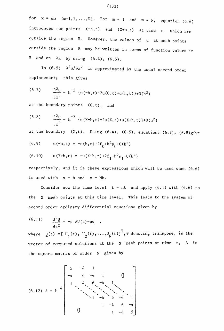
(I33)
for x = mh (m=1,2 •... ,N). For m = 1 and m = N, equation (6.6)
introduces the po1.·nts (-h t) and (X+h t) ., ~ at t1me t. which are
outside the reg1.on R. However, the values of u at mesh points
outside the reg1.on R may be written in terms of function values 1n
R and on aR by using (6.4), (6.5).
In (6.5) a2u/ax2 1.S approximated by the usual second order
replacement; this gives
(6.7) -2= h {u(-h,t)-2u(0,t)+u(h,t)}+0(h2)
(6.8)
at the boundary points (O,t), and
a2u -2--- - h {u(X-h,t)-2u(X,t)+u(X+h,t)}+0(h2)ax 2
at the boundary (X,t). Using (6.4), (6.5), equations (6.7), (6.8)give
(6.9)
(6.10)
respectively, and it 1.S these expressions which will be used when (6.6)
1S used with x = h and x = Nh.
Consider now the time level t = n£ and apply (6.1) with (6.6) to
the N mesh points at this time level. This leads to the system of
second order ordinary differential equations given by
(6.11) ,
whereT. . h"Q(t) =[ U
1(t ) , U
2(t),... ,U
N(t)],T deno t i.ng transpose, 1.S t e
vector of computed solutions at the N mesh points at time t, A 1.S
the square matrix of order N g1.ven by
(6 . 12) A = h-4
5 -4
-4 6 -4 0-4 6 -4... .... ... ........ .... .... .... " ........ .... .... ...
.... ".... "....
" "....
"" .... .... "" ....... " ......-4 " 6 -4" 1
-4 6 -4
0 -4 5
(134)
with eigenvalues
(6.13)
and w
(6.14)
-4As = 16 h sin
4[ sn/{2(N+l)}]; s = 1,2, ... ,N
1S the vector of boundary values of order N g1ven by
w = h-4[
h2PO-2fO.fO.O •.•• ,O.f].h2p -2f1] T
Solving (6.11) subject to the initial conditions (6.2), (6.3) g1ves
(6.15) U(t) A- I I (Lv t B) -1-1- = - ~+ zexp 1ytB {&O+(iytB) &1+A w}
in which i = Nl, y = /1..1 and B . 2vu 1S a matr1x such that B = A.
It is easy to show that (6.15) satisfies the recurrence relation
(6.16) ~(t+t) - {exp (iytB)+exp(-iytB)}~(t)+~(t-t)
-1 -1= {exp (iytB)+exp(-iytB)}A ~-2A ~
with t = t,2t, ... and it is this relation which will be used 1n the
development of the family of algorithms for solving (6.1) with (6.2),
(6.3), (6.4), (6.5). It will not be necessary to compute y, B or-1
A explicitly.
6.3 Solution at the first time step
It is clear that, using (6.15) with t = t, requ1res knowledge of
~(t) which, unlike ~(O), is not contained explicitly in the initial
conditions. Writing t = t in (6.15) and replacing the matrix expo-
nentia1 functions with xheir (0,3) Pade approximants leads to
(6.17)
replacing the matrix exponential functions with their (0,5) Pade
approximants leads to
(6.18) ~(t) = (1- .!..1..1 £, 2A+ _1_ 1..1 2 £, 4A2) s + £, (I - ~ £, 2A~1..12 t 4A2) g2 24 ° 6 120 1
_ .!..lIt2 (1- _1 1..I£,2A)w+0(£,6)2 t-" 12 -
and uS1ng the (0,7) Pade approximants leads to
(135)
(6.19)
In problems having time dependent boundary conditions f O,f 1,PO,P1,
(6.4), (6.5) func;tions of~n are t and the vector w ~n (6.17), (6.18),-(6.19) .
evaluated,
~s us~ng t :::: £ ~n the equation
(6.20)
The complete algorithm for computing the numerical solution of (6.1)
with (6.2), (6.3), (6.4), (6.5) may thus be listed as follows:
(i) the starting vector U_(O):::: go 's obta~ned fr t' (6 2)~ ~ om equa ~on . ;
(ii) the starting vector g(£) is obtained using (6.17), (6.18) or
(6.19) depending on the required accuracy;
(iii) ~(t+£), with t:::: £,2£, ... , ~s obtained from the recurrence
relation (6.16) in which the matrix exponential functions are
replaced by suitable approximants. It is these matrix functions
which will be replaced by Pade approximants in the next section.
6.4 Development and analyses of the methods
Using the (1,1) Pade approximants to the matrix exponential
functions in (6.16) leads to a difference scheme written in matrix form as
(6.21)
for problems with time dependent boundary conditions this becomes
(6.22)
part of the loca l truncation error of the method basedThe principal
on the (1,1) Pade approximant is given by
(6.23)
(136)
of (6.23) 1S related to the space dis-The componentdX6
cretization and the use of (6 6)· (6 1)• 1n • ; this component will be
present in all methods derived by using Pade approximants to the matrix
exponential function in (6.16). The other component of (6.23) is re-
lated only to the Pade approximant chosen for use in (6.16). The
principal part of the local truncation error of any method arising from
the use of the (m,k) Pade approximant in (6.16) will thus have the form
(6.24)
where the C (q = m+k+1 for m + k odd, and q = m+k+2 for m + kq
even) are error constants and are given in Appendix III. All Pade
approximants except the (0,1), (1,0) approximants lead to consistent
methods.
Stability, in the conventional sense of a perturbation of the initial
data not growing in magnitude as time increases, is analysed by recourse
to the stability equation of the method.
Noting that the (m,k) Pade approximant to the matrix exponential
function exp (iytB) has the form
(6.25) exp (iy tB) = [ ~ (iYtB)] -1 . P (iytB)+0(tm+k+ 1)k
where Pk'~ are polynomials of degrees k and m, respectively, with
PO(iytB) = I and QO(iytB) = I (I is the identity matrix of order N),
the stability equation has the form
(6.26)
In (6.26), f A d ~ 1S the amplification factor1S an eigenvalue 0 an ~
of the method. The von Neumann necessary condition for stability
(6.27)
hence requires,
(137)
In the case of the method based on the ( 1,1) Pade approximant,
the stability equation is
(6.28)
and it 1S found that IeI~ 1 for any r = t/h2 ~ O· 0S1nce ~ > , A > O.
The scheme is therefore unconditionally stable.
Using the (0,2) Pade approximant in (6.16) the resulting finite
difference method for problems with time dependent boundary conditions may
be written in vector form as
(6.29)
This is the explicit scheme of Collatz (1951) for which This
method has an error constant which is the same order as that of (6.22)
and, since it is explicit, it would appear to be a more desirable method
to use. It is, however, stable only for1
r ~ ~ and may thus be used
only with small time steps.
Turning now to the (1,2) Pade approximant, its use 1n (6.16)
yields the method
(6.30)
so that the methodC = -1/36,4
enJoys better accuracy than (6.22) or (6.29). Its stability equation
The method is second order accurate with
yields the restriction ~t2A ~ 36/5 which, since A < 16h-4 , leads to
the stability condition r ~ 3/5 /(10~). Thus it may be used with
slightly bigger time steps than (6.29). However, the fact that it is
implicit, does not make this method more attractive than (6.22) which,
though implicit, is unconditionally stable.
A notable improvement in the accuracy in time 1S obtained by uS1ng
the (2,2) Pade approximant to the matrix exponential functions in (6.16).
(L:H:S)
This approximant gives the method
(6.31)
for which
(1+ 112
lJ Q,2A+ 14
14lJ 2Q, 4A2)!:! (t +Q, ) + ( _1_ uQ, 21+ _1_11 2 Q, 4A)w
12 144 -t+£
== (21- 26 ll Q, 2 A+ 7121-l2£4A2)U(t)_(~]JQ,2I+ _1 lJ2Q,4A)w- 6 72 -t
- (1+ TI ]JQ, 2A+ 1~4112Q,4A2)!:!(t-Q,)-( TzlJ£2I+ 114 lJ 2Q,4A)wt_£
1C6== 360 (from Appendix III). The stability equation 1S
(1+112llQ,2A+1Z4lJ2 Q,4A2)~2_(2- ~lJQ,2A+ _1 112Q,4A2)c+(1+ _1_lJQ,2 A+ _1 lJ2£4,\2) ==. .' 6 72 <:. 12 144
from which it 1S found that the method is unconditionally stable.
Squaring the matrix A involves an increase in the number of mesh
points at each time level used in the computation. This notion of uS1ng a
greater number of points at each time level was used by Khaliq and Twizell
(1982) for first order hyperbolic partial differential equations and by
Twizell (1979) for second order hyperbolic partial differential equations~
Mitchell and Griffiths (1980) discussed the concept briefly for second
order parabolic partial differential equations.
The same order of accuracy in time may be achieved by deleting the
terms in A2 from (6.31); this gives
(6.31a)
for which c == 1/240.6
Equation (6.31a) is, in fact, an application of
Numerov's linear multi~step method for the numerical solution of a system
of second order ordinary differential equations and the finite difference
scheme resulting from it for the solution of (6.1) is stable only for
lJ r 2 ~ 3/8. Equation (6.31a) may be useful when very small time steps may
be taken.
The (2,1) Pade approximant leads to the implicit method
(6.32)
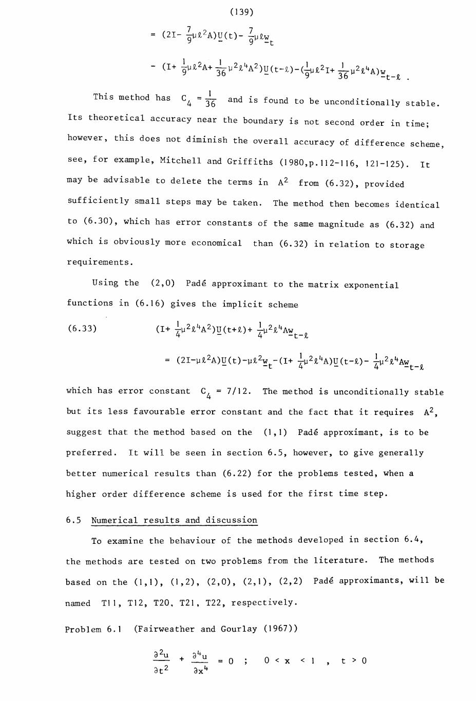
(139)
= (21- 79~£2A)U(t)- ~~£w- 9-t
- (1+ -§vQ, 2A+ 316
u 2Q, 4A2)U (t-£) - (~£2I+ _1_~2 £4A)w- 9 36 -t-£ .
This method has =_1C4 36 and is found to be unconditionally stable.
Its theoretical accuracy near the boundary is not second order in time;
however, this does not diminish the overall accuracy of difference scheme ,
see, for example, Mitchell and Griffiths (1980,p.112-116, 121-125). It
may be advisable to delete the terms in A2 from (6.32), provided
sufficiently small steps may be taken. The method then becomes identical
to (6.30), which has error constants of the same magnitude as (6.32) and
which is obviously more economical than (6.32) in relation to storage
requirements.
Using the (2,0) Pade approximant to the matrix exponential
functions In (6.16) gives the implicit scheme
(6.33)
which has error constant C4
= 7/12. The method is unconditionally stable
but its less favourable error constant and the fact that it requires
suggest that the method based on the (1,1) Pade approximant, is to be
preferred. It will be seen in section 6.5, however, to give generally
better numerical results than (6.22) for the problems tested, when a
higher order difference scheme is used for the first time step.
6.5 Numerical results and discussion
To examine the behaviour of the methods developed in section 6.4,
the methods are tested on two problems from the literature. The methods
b d h (1 I) ( 1 2) (2 0) (2 I) ( 2 2) Pade approximants, wi 11 bease on t e , , , , , , , , ,
named Tl I, T12, T20, T21, T22, respectively.
Problem 6.1 (Fairweather and Gourlay (1967))
= ° ° < x < 1 , t > 0
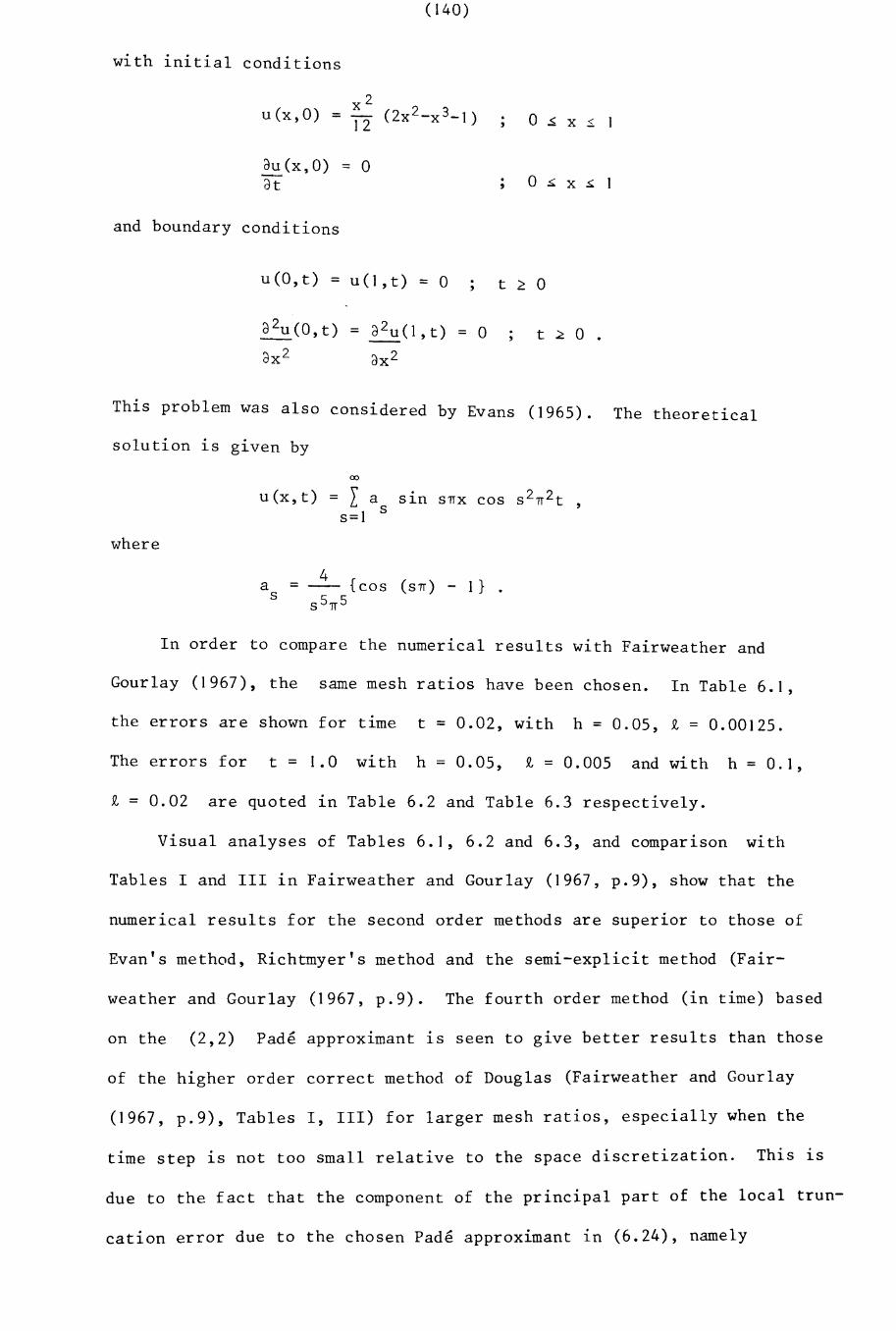
(140)
with initial conditions
~(x,O) = 0at
and boundary conditions
., o ~ x ~ I
u(O,t) = u(l,t) = 0 t ~ 0
a2u (0 , t ) =
ax 2
a2u ( l , t ) = 0
ax2t ~ 0 .
This problem was also considered by Evans (1965). The theoretical
solution is given by
00
where
as
In order to compare the numerical results with Fairweather and
Gourlay (1967), the same mesh ratios have been chosen. In Table 6.1,
the errors are shown for time t = 0.02, with h = 0.05, t = 0.00125.
The errors for t = 1.0 with h = 0.05, t = 0.005 and with h = 0.1,
£ = 0.02 are quoted ~n Table 6.2 and Table 6.3 respectively.
Visual analyses of Tables 6.1, 6.2 and 6.3, and comparison with
Tables I and III in Fairweather and Gourlay (1967, p.9), show that the
numerical results for the second order methods are superior to those of
Evan's method, Richtmyer's method and the semi-explicit method (Fair-
weather and Gourlay (1967, p.9). The fourth order method (in time) based
on the (2,2) Pade approximant is seen to give better results than those
of the higher order correct method of Douglas (Fairweather and Gourlay
(1967, p.9), Tables I, III) for larger mesh ratios, especially when the
time step is not too small relative to the space discretization. This is
due to the fact that the component of the principal part of the local trun-
cation error due to the chosen Pade approximant in (6.24), namely
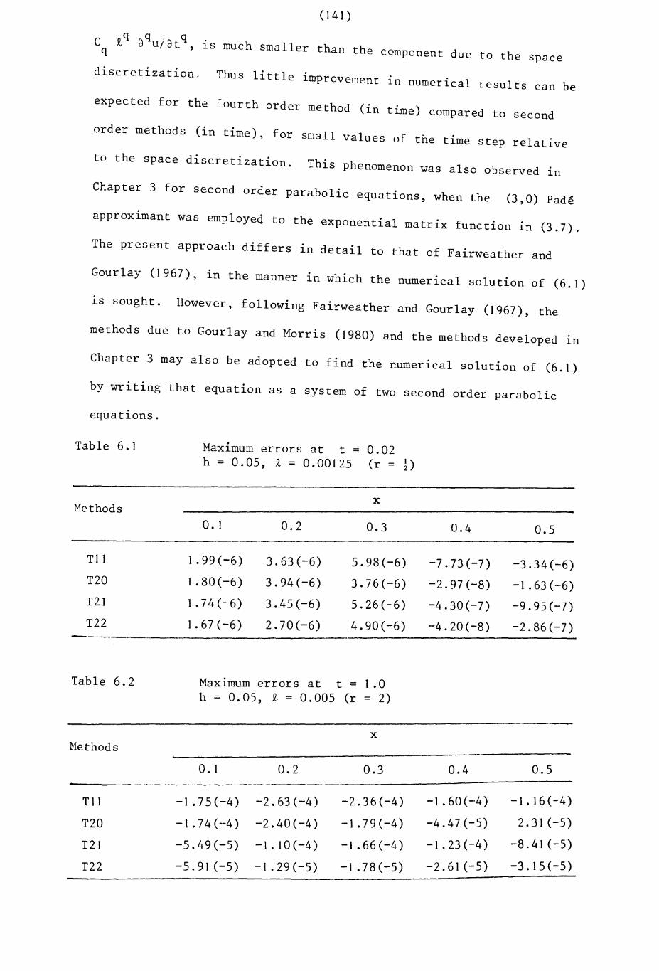
(141 )
c tq
aquiatq,
is much smaller than the component due to the spaceq
discretization. Thus little improvement in numerical results can be
expected for the fourth order method (in time) compared to second
order methods (in time), for small values of the time step relative
to the space discretization. This phenomenon was also observed 1n
Chapter 3 for second order parabolic equations, when the (3,0) Pade
approximant was employeq to the exponential matrix function in (3.7).
The present approach differs in detail to that of Fairweather and
Gourlay (1967), in the manner in which the numerical solution of (6.1)
is sought. However, following Fairweather and Gourlay (1967), the
methods due to Gourlay and Morris (1980) and the methods developed 1n
Chapter 3 may also be adopted to find the numerical solution of (6.1)
by writing that equation as a system of two second order parabolic
equations.
Table 6.1
Methods
TIl
T20
T21
T22
Maximum errors at t = 0.02h = 0.05, £ = 0.00125 (r = !)
x
O. 1 0.2 0.3 0.4 0.5
1.99(-6) 3.63(-6) 5.98(-6) -7.73(-7) -3.34(-6)1.80(-6) 3.94(-6) 3.76(-6) -2.97(-8) -1.63(-6)1.74 (-6) 3.45(-6) 5.26(-6) -4.30(-7) -9.95(-7)
1.67 (-6) 2.70(-6) 4.90(-6) -4.20(-8) -2.86(-7)
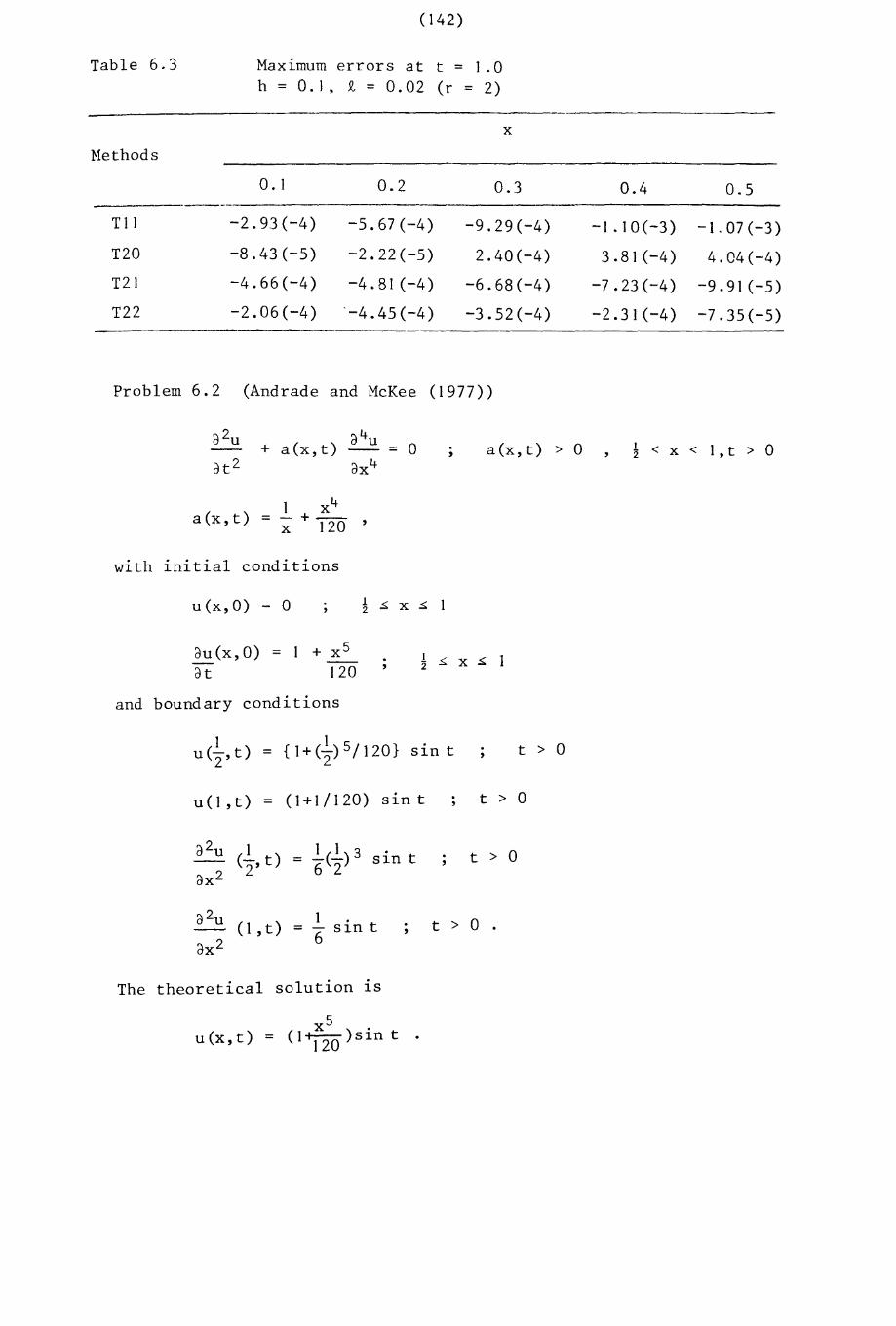
Table 6.3
Methods
( 142)
Maximum errors at t = 1.0h = 0.1. ~ = 0.02 (r = 2)
x
O. I 0.2 0.3 0.4 0.5
TIl -2.93(-4) -5.67(-4) -9.29(-4) -1.10(-3) -1.07(-3)
T20 -8.43(-5) -2.22(-5) 2.40(-4) 3.81 (-4) 4.04(-4)T21 -4.66(-4) -4.81 (-4) -6.68(-4) -7.23(-4) -9.91 (-5)
T22 -2.06(-4) "-4.45(-4) -3.52(-4) -2.31(-4) -7.35(-5)
Problem 6.2 (Andrade and McKee (1977))
a(x,t)1 x4
= - +--x 120'
., a(x,t) > 0 ~ < x < l,t > 0
with initial conditions
u(x,O) = 0
au(x,O) = 1 + x 5
at 120
and boundary conditions
1 {1+(~)5/120} sin t t > 0u (2' t ) =
u(l,t) = (1+1/120) sin t t > 0
a2u 1 1-(1-)3 sin t t > 0("2' t ) =ax 2 6 2
1 •= - s Lfl t6
., t > 0 .
The theoretical solution is
x 5u(x,t) = (lm)sin t .
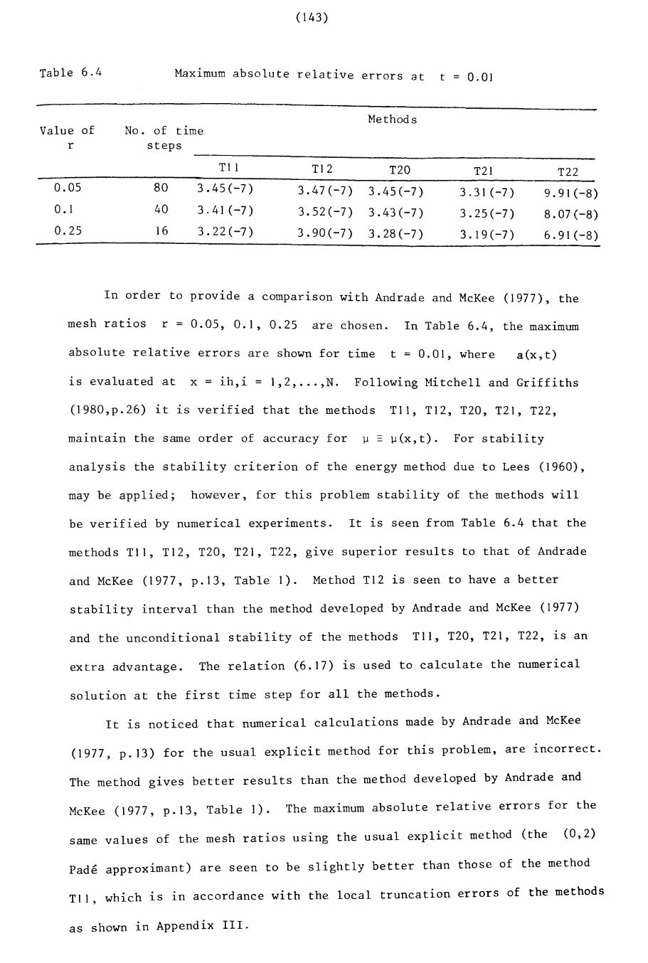
Table 6.4
(143)
Maximum absolute relative errors at t = 0.0]
MethodsValue of No. of time
r steps
Til T12 T20 T2] T220.05 80 3.45(-7) 3.47(-7) 3.45(-7) 3.31 (-7) 9.91(-8)O. 1 40 3.41 (-7) 3.52(-7) 3.43(-7) 3.25(-7) 8.07(-8)0.25 16 3.22 (-7) 3.90(-7) 3.28(-7) 3.19(-7) 6.91(-8)
In order to provide a comparison with Andrade and McKee (1977), the
mesh ratios r = 0.05, 0.1, 0.25 are chosen. In Table 6.4, the maximum
absolute relative errors are shown for time t = 0.01, where a (x , t )
is evaluated at x = ih,i = 1,2, ... ,N. Following Mitchell and Griffiths
(1980,p.26) it is verified that the methods TIl T12 T20 T21 T22, , , , ,
maintain the same order of accuracy for ~ = ~(x,t). For stability
analysis the stability criterion of the energy method due to Lees (1960),
may be applied; however, for this problem stability of the methods will
be verified by numerical experiments. It is seen from Table 6.4 that the
methods TIl, T12, T20, T21, T22, g1ve superior results to that of Andrade
and McKee (1977, p.13, Table 1). Method T12 1S seen to have a better
stability interval than the method developed by Andrade and McKee (1977)
and the unconditional stability of the methods TIl, T20, T21, T22, is an
extra advantage. The relation (6.17) is used to calculate the numerical
solution at the first time step for all the methods.
It is noticed that numerical calculations made by Andrade and McKee
(1977, p.I3) for the usual explicit method for this problem, are incorrect.
The method gives better results than the method developed by Andrade and
McKee (1977, p.I3, Table 1). The maximum absolute relative errors for the
same values of the mesh ratios using the usual explicit method (the (0,2)
Pade approximant) are seen to be slightly better than those of the method
TIl, which is in accordance with the local truncation errors of the methods
as shown in Appendix III.
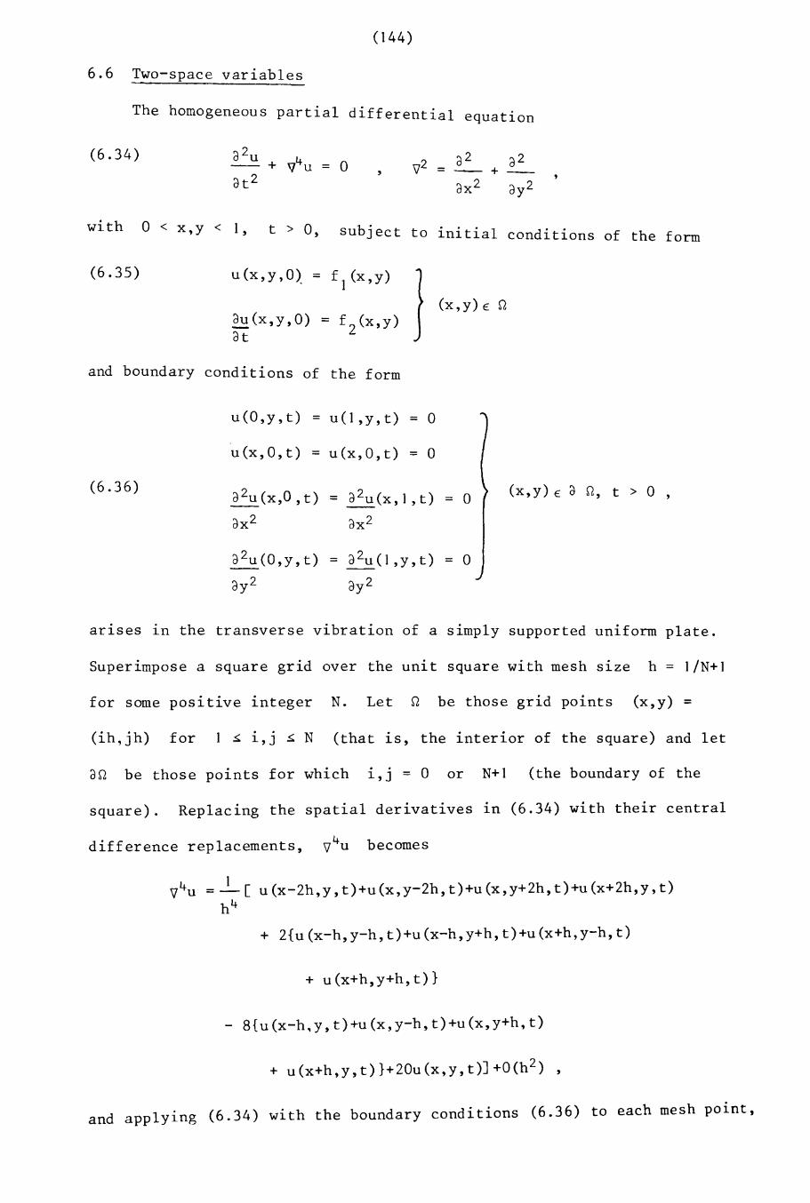
(144)
6.6 Two-space variables
The homogeneous partial differential equation
(6.34) a2uV4u ° IJ2 a2 a2-- + = = -- +
at 2ax 2 ay2
with ° < x,y < 1, t > 0, subject to initial conditions of the form
(6.35) u(x,y,O) = f1
(x,y)
au(x,y,O) = f2(x,y)at
(x,y) E n
and boundary conditions of the form
u(O,y,t) = u(I,y,t) = °u (x , 0, t) = u(x,O,t) = °
(6.36)a2u (x,O ,t) a2u(x,1,t) (x,y) E a n, t > °= = 0 ,
ax 2 ax 2
a2u (0, y, t ) = a2u (1 ,y, t ) = °ay 2 ay 2
ar1ses 1n the transverse vibration of a simply supported uniform plate.
Superimpose a square grid over the unit square with mesh S1ze h = I/N+1
for some positive integer N. Let n be those grid points (x,y) =
(ih,jh) for 1 ~ i,j ~ N (that is, the interior of the square) and let
an be those points for which 1,J = ° or N+1 (the boundary of the
square). Replacing the spatial derivatives in (6.34) with their central
difference replacements, IJ4u becomes
IJ4u = _1_ [ u (x-2h,y, t)+u(x,y-2h, t)+u (x,y+2h, t)+u (x+2h,y, r )h 4
+ 2{u(x-h,y-h,t)+u(x-h,y+h,t)+u(x+h,y-h,t)
+ u(x+h,y+h,t)}
- 8{u(x-h.y,t)+u(x,y-h,t)+u(x,y+h,t)
+ u(x+h,y,t)}+20u(x,y,t)J+O(h2 ) ,
and applying (6.34) with the boundary conditions (6.36) to each mesh point,
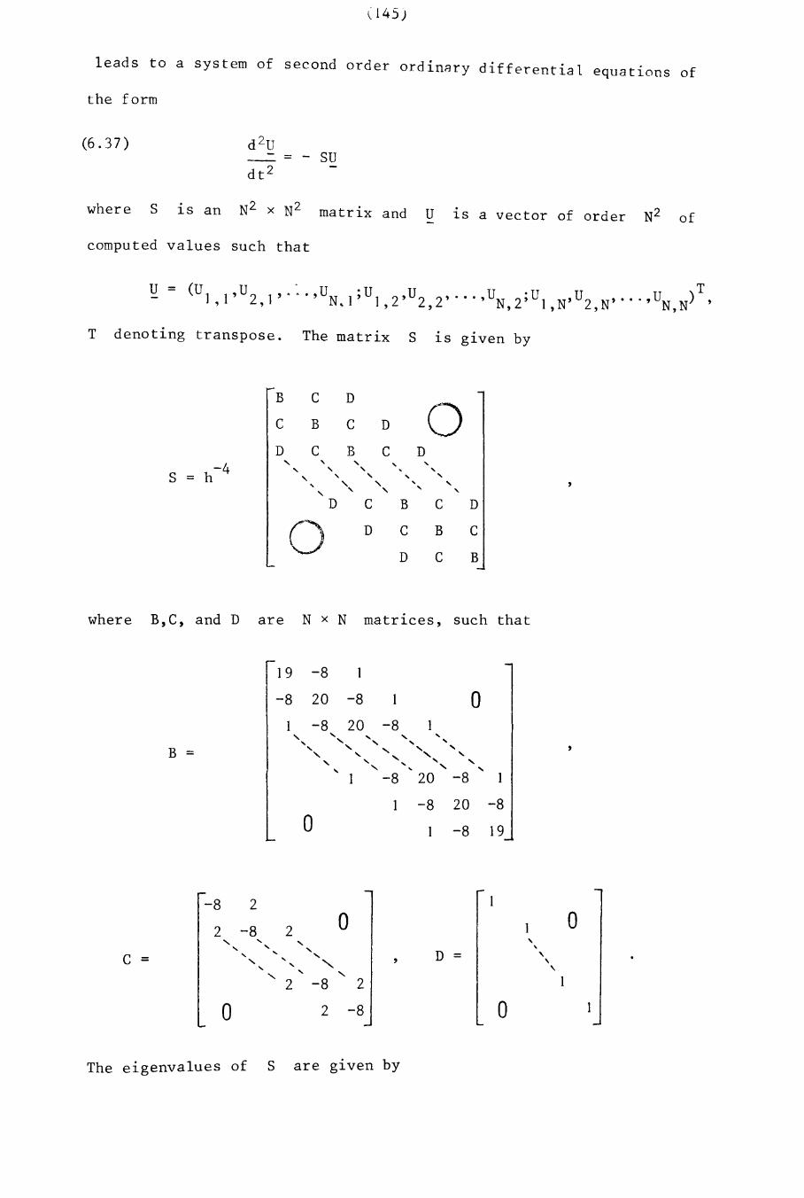
(145 )
leads to a system of second order ordinary differential equations of
the form
(6.37 )= su
where S 1S an N2 x N2 matrix and U 1S a vector of order N2 of
computed values such that
T denoting transpose. The matrix S 1S g1ven by
B C D
0C B C D
D C B C D"
," , ,
-4 ", , ,, , , ....S = h " " -, ,
",.... "
.... ," D C B C D
0 D C B C
D C B
where B,C, and Dare N x N matrices, such that
19 -8
-8 20 -8 o
B =
1 -8 20 -8" " "
, ........ " , .... ....
" " " ",
-, " "" " ," " ....
"-, , ........-8 20 -8
-8 20 -8a -8 19
-8 2 o....,,,,
o
D =
2
o
2 -8
,", <,
<,
-8
2
, 2
a
2 -8" ...." ........ "-" ........ .... ....C =
The eigenvalues of S are g1ven by
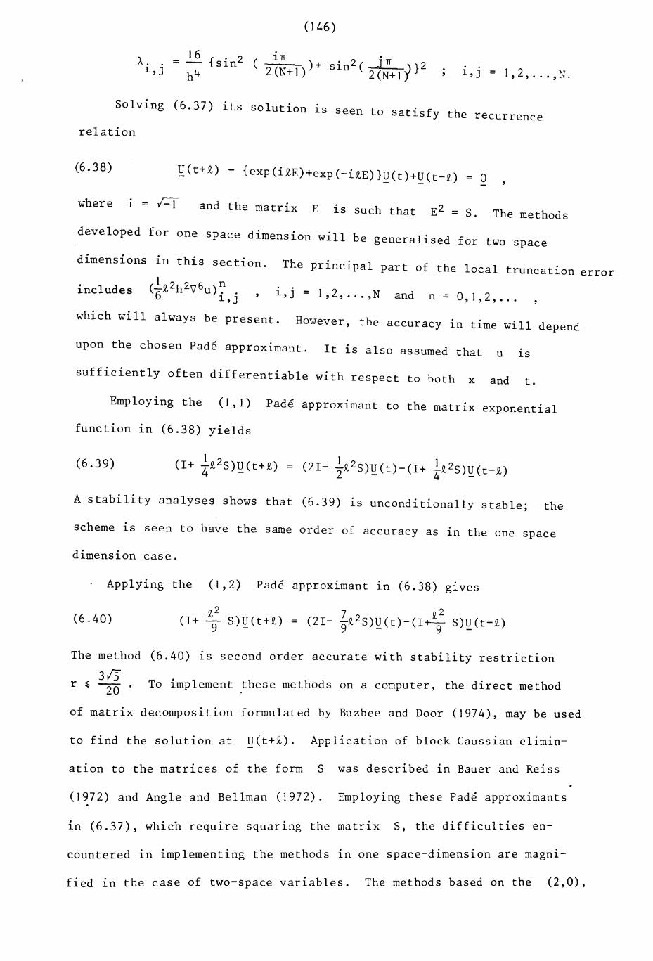
(146)
A = 16 {S l'n2 ( 1TI 2 j TIi,j h" 2(N+I))+ sin (2(N+lt}2 i,j = 1,2, ... ,~.
Solving (6.37) its solution 1S seen to sat1'sf thy e recurrence
relation
(6.38) ~(t+£) - {exp(i£E)+exp(-i£E)}~(t)+~(t_£) = 0
where i = I=Tand the matrix E 1S such that E2 = S. The methods
developed for one space dimension will be generalised for two space
dimensions in this section. The principal part of the local truncation error
includes , i,J' = 1,2, ... ,N and n = 0 1 2, , , ...which will always be present. However, the accuracy in time will depend
upon the chosen Pade approximant. It is also assumed that u 1S
sufficiently often differentiable with respect to both x and t.
Employing the (1,1) Pade approximant to the matrix exponential
function in (6.38) yields
(6.39)
A stability analyses shows that (6.39) is unconditionally stable; the
scheme is seen to have the same order of accuracy as in the one space
dimension case.
Applying the (1,2) Pade approximant 1n (6.38) glves
(6.40)
The method (6.40) is second order accurate with stability restriction
r ~31520 . To implement these methods on a computer, the direct method
of matrix decomposition formulated by Buzbee and Door (1974), may be used
to find the solution at Q(t+£). Application of block Gaussian elimin-
ation to the matrices of the form S was described in Bauer and Reiss
(1972) and Angle and Bellman (1972). Employing these Pade approximants
in (6.37), which require squaring the matrix S, the difficulties en-
countered in implementing the methods 1n one space-dimension are magni-
fied in the case of two-space variables. The methods based on the (2,0),
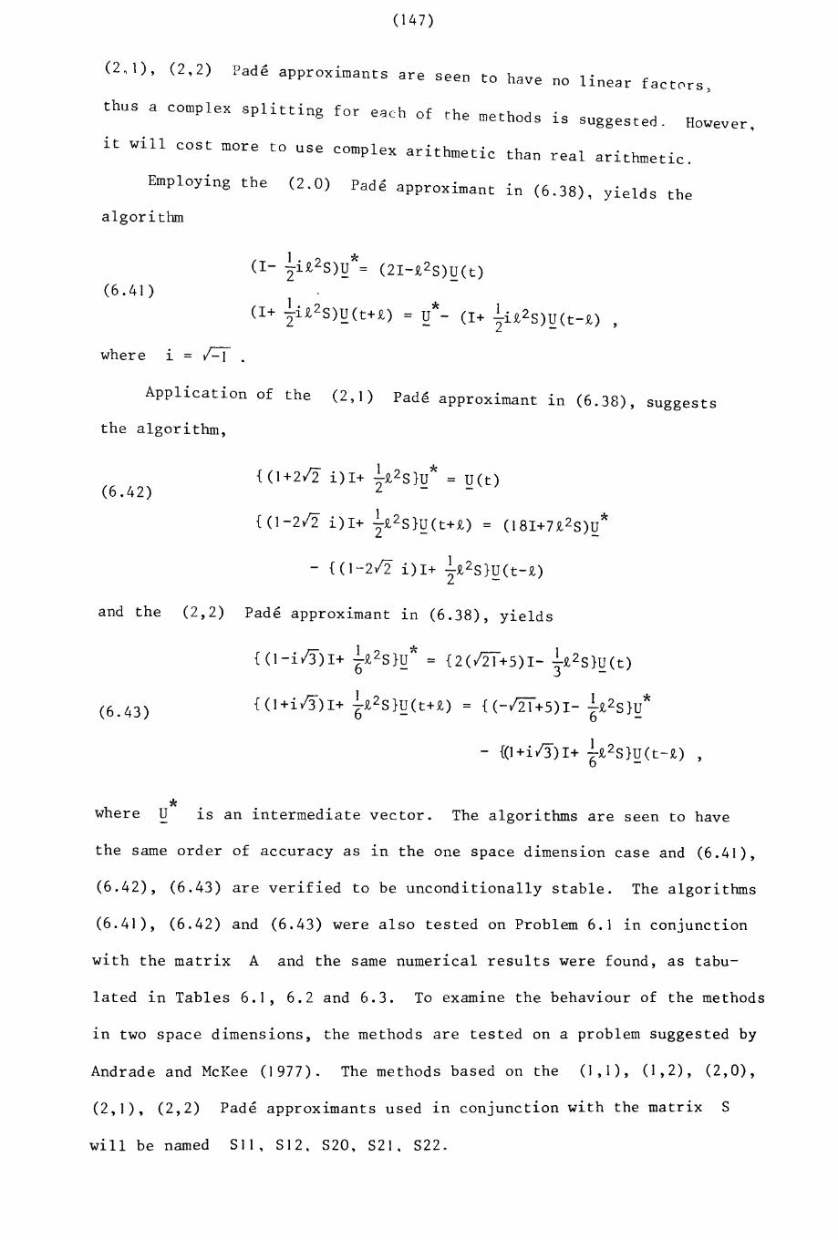
(2 0 1) , (2,2)
(147)
Pade approX1mants are seen to have no linear fact0rs ,thus a complex splitting for each of the methods 1S
suggested. However,
it will cost more to use complex ar1·thmet1·c than real arithmetic.
Employing the (2 0) P d ~ .. a e apprOX1mant in (6.38), yields the
algorithm
(6.41)
(1+ l-i.Q,2S)U (t-.Q,)2 -
where i = /=T .
Application of the (2,1) Pade approximant 1n (6.38), suggests
the algorithm,
(6.42){(I+Z/2 i)1+ l-.Q,2 S}U* = U(t)
2 - -
{(I-Z/2 i)1+ ~.Q,2S}~(t+.Q,) = (181+7.Q,2S)~*
- {(1-2/2 i)I+ l-.Q,2S}U(t-.Q,)2 -
and the (2,2) Pade approximant in (6.38), yields
(6.43)
{(I-i!3)I+ 61.Q,2S}~* = {Z(I21+5)1- l-.Q,2S}U(t)3 -
{(I+i!3)1+ 61.Q,2S}~(t+.Q,) = {(-121+5)1- l-.Q,2S}U*6 -
- «1+il3)1+ ~.Q,2S}~(t-.Q,)
*where U 1S an intermediate vector. The algorithms are seen to have
the same order of accuracy as in the one space dimension case and (6.41),
(6.42), (6.43) are verified to be unconditionally stable. The algorithms
(6.41), (6.42) and (6.43) were also tested on Problem 6.1 in conjunction
with the matrix A and the same numerical results were found, as tabu-
lated in Tables 6.1, 6.2 and 6.3. To examine the behaviour of the methods
in two space dimensions, the methods are tested on a problem suggested by
Andrade and McKee (1977). The methods based on the (1,1), (1,2), (2,0),
(2,1), (2,2) Pade approximants used in conjunction with the matrix S
will be named SII, S12. S20, S21. S22.
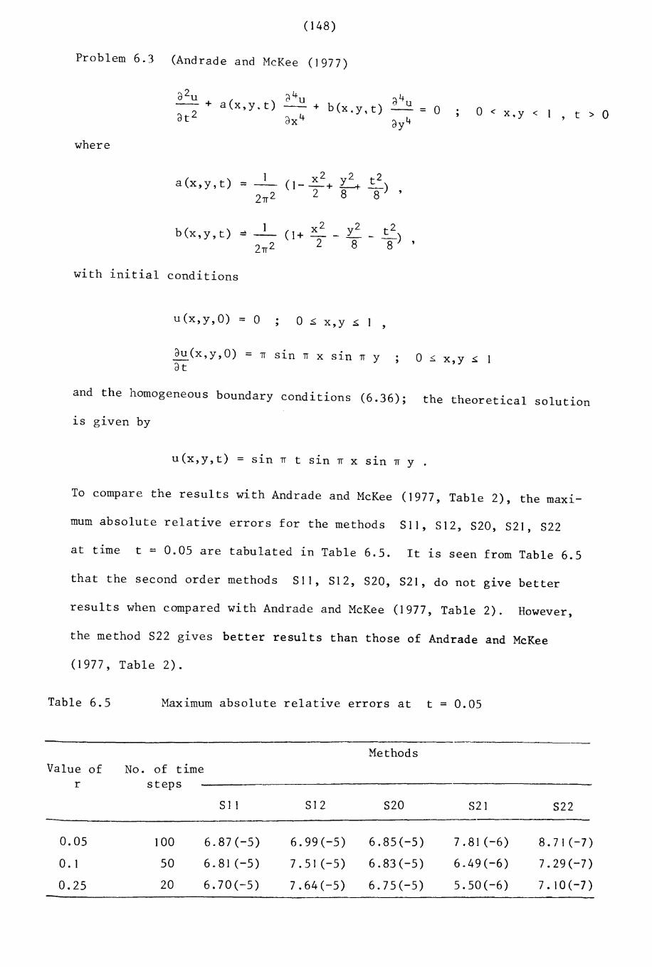
(148 )
Problem 6.3 (Andrade and McKee (J977)
o < x.y < 1 , t > 0
where
a(x,y,t) =
b(x,y,t) ==
with initial conditions
X 2 2(1+ - - Y
2 8
u(x,y,O) = 0 o s x,y .:s; 1 ,
dU(X,y,O) = n Sln n x Sln n y 0 .:s; x,y .:s; 1dt
and the homogeneous boundary conditions (6.36); the theoretical solution
is given by
u(x,y,t) = .Sln n t Sln n x Sln n y .
To compare the results with Andrade and McKee (1977, Table 2), the maXl-
mum absolute relative errors for the methods 811, 812, 820, 821, 822
at time t = 0.05 are tabulated in Table 6.5. It is seen from Table 6.5
that the second order methods 811, 812, 820, 821, do not glve better
results when compared with Andrade and McKee (1977, Table 2). However,
the method 822 gives better results than those of Andrade and McKee
(1977, Table 2).
Table 6.5 Maximum absolute relative errors at t = 0.05
MethodsValue of No. of time
r steps
81 1 812 820 821 822
0.05 100 6.87(-5) 6.99(-5) 6.85(-5) 7 .81 (-6) 8.71(-7)
O. 1 50 6.81 (-5) 7.51(-5) 6.83(-5) 6.49(-6) 7.29(-7)
0.25 20 6.70(-5) 7.64(-5) 6.75(-5) 5.50(-6) 7.10(-7)
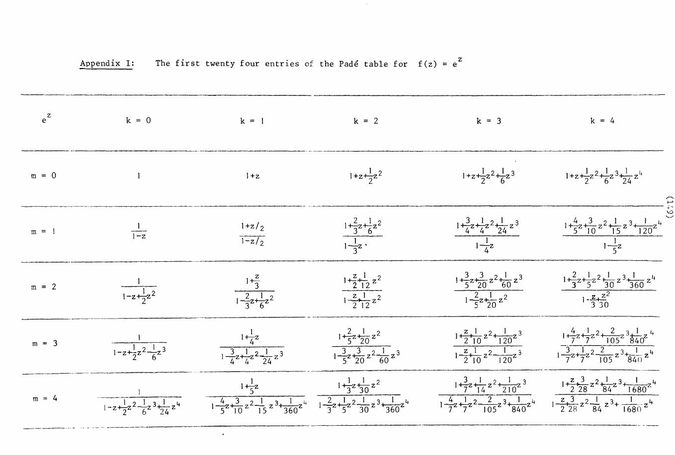
Appendix I: The first twenty four entries of the Pade table for f(z)z= e
ze k = 0 k = k = 2 k = 3 k = 4
In = 0 1 l+z l+z~z2 1 2 1 1+zJ..z2.J.z 3?- z"1+z+-z +-:-z 32 6 2 6 24
~
~4 .......'0
2 1 3 1 21 3 4 3 2 1 3 ) 4'-./
1 l+z/ 2 1+-z+-z2 l+t;z7 '24 z )+-z+-z +-z +--zIn = I -- 3 6 5 10 15 120
I-z1-z/2 1 I 1
1-z' 1-z I-z3 4 5
H-j- z 1 2 3 3 1 3 2 I ) 1
In = 21 l+z+- Z 1+-z+-- z 2+:--,,- z I+-z+-z2+_- z 3+- z "
1-z~212 5 20 60 3 5 30 360
21 2 z 1 2 21 2 22 1-z+-z 1 2....12 Z I-z+--z )-~
3 6 5 20 3 30~ -
1 2 1 z I 2 1 3 41 22 3 1 4
In = 3I I~z 1+sz '20 z2 11 2110
z +rnz )+-tz+-:p ~z 840z
l-z?z2--'!"z3 3 1 1 3 3 3 2 1 3 z 1 2 1 3 1 3z+l.-z22..- z 3+_~ z 42 6 l-z+-:-z2-zISZ '20 z 60 z 12~z I20z
4 4 24 7 7 lOS 840-
1 1 1 2 3 I 2 1 3 z3 2) 3 14It-sz 17'30 z 1+r+t4 z mz )t, z+-z+ z
1 2 28 84 )680In = 4
I-z+-k 2_1z 3.J- z 4 43 2 13 14 21 2 13 1 4 41 22 3 1 4 z3 21314ISZ~Z Is z 1360z 13"zt-sz 30 z 1360 z 17+r IOSz 1840 z I 2 '28 z 84 z + 1680- z
2 6 24
---- ---- ._----
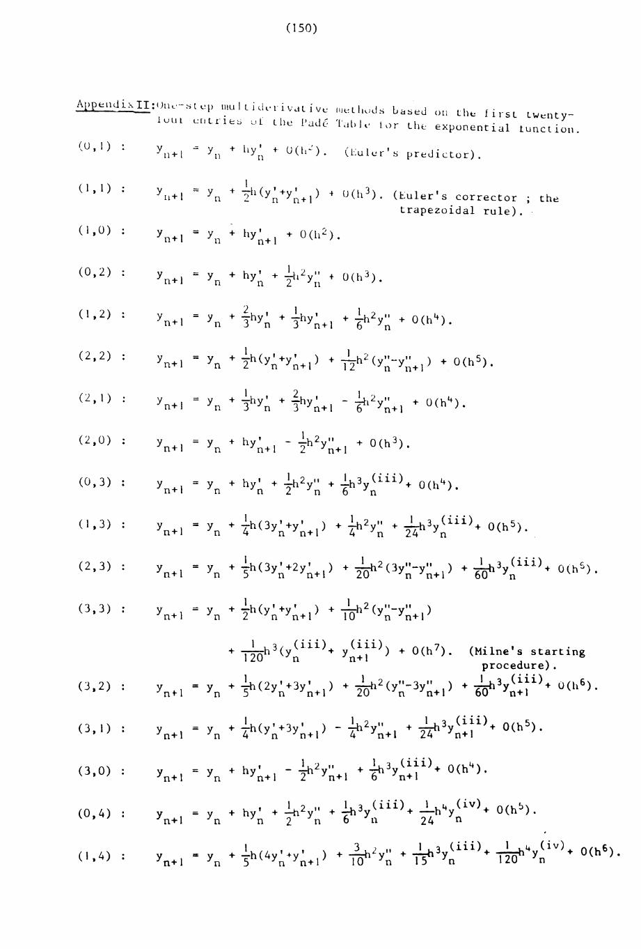
(150)
APPt:llJi:-"II:(JL1,-·--~tq) lllullidvrlVdlivl: Illl:lltl.;ds Ld~eJ• OIl tht; first lWenty-
Lo u t cu t. r i e s oI tile PadC: 'LJl>l,' lo r tIl'-''- exponential tunctioll.
(U,I) y .;;; y + by' t U(h..:').tl+l II n (Euler's predictor).
( 1 , I )
( I , 0)
( I ,2)
(2,2)
(2, I )
(2,0)
(0,3)
( I ,3)
(2,3)
(3,3)
IYll+1
;;;
Yn + -;-h(y'+y' ) -t U(h 3 ) . (Euler's2 n n+1 corrector , thetrapezoidal rule).
Yn+1 = Yn + hy' + 0(11 2 ) .n+1
Yn+ 1;;; Yn
+ hy' + It 2 " + 0(h 3 ) .n "2 1 Yn
Yn+1;;;
Yn + 2 h ' I h ' + ~h2 " + 0(h 4 ) .3" Yn + - Y3 n+l 6 Yn
1_I_h 2 ( " _" )Yn+ 1
;;;
Yn + "2h(y' +y' ) + + O(h S).n n+1 12 Yn Yn+ 1
Yn+ 1 = Yn+ I h ' + lh ' ~12y" + 0(h 4 ) .3" Yn 3 Yn+ 1 6 n+l
Yn+ 1 = Yn+ h ' I h 2 " + 0(h 3).
Yn+ 1 "2 Yn+ 1
;;; Y + h Y, + I h 2 II + ~h 3Y( iii) + 0 (h 4) •n n"2 Yn 6 n
= Y + ~h(3y' +y' ) + ~2y" + ~h3 (iii) O(hS)n 4 n n+1 4 n 24 Yn + •
= Yn
+ ~h(3Y'+2y' ) + ~2(3y"-Y" ) + ~3 (iii)+ O(hS).5 n n+1 20 n n+1 60 Yn
= + ~h(y' +y' ) + ~2 (y"-y" )Yn 2 n n+l 10 n n+l
(3,2)
+ 1 h 3( (iii)+ (iii» + 0(h7).120 Yn Yn+ 1
Y = Y + -:-hSI
(2y'+3y' 1) + ~2(Y"-3y" )n+1 n n n+ 20 n n+l
(Milne's startingprocedure).
+ ~3y(iii)+ 0( 6 )60 n + 1 l.
(3, 1)
(3,0)
(0,4)
( 1 ,4)
= Y + 41h(y'+3Y' 1) - ~2y" + ~3y(iii)+ O(h S).n n n+ 4 n+l 24 n+l
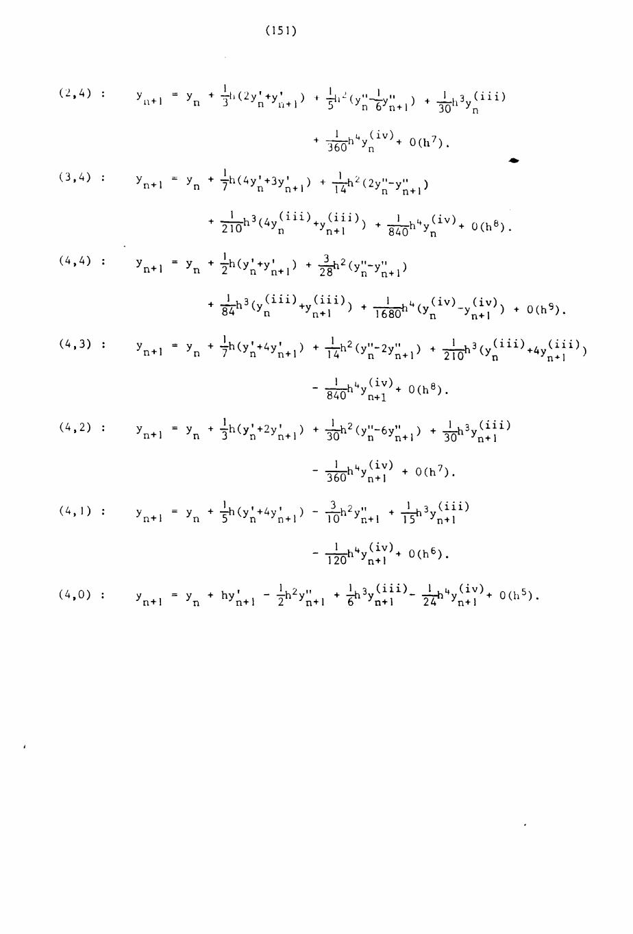
Yn + 1
(151)
1= Y + -:7-I.J
I ( 2Y, +y , ) +n n n+ 1 ~ I .: (Y" -.2-y " ) +..1...1 3 (i i i )
5 n 6 n+ 1 30 1 Yn
+ 1 h 4 (i v ) 0 (117) •J60 Yn +
Yn + 1 ;; Yn + .!..h ( 4 Y, +3Y, ) +~ 2 ( 2Y"-YII )
7 n n+ 1 14 n n+ 1
..
Yn + 1 = Y + .!..h(y' +y' ) + k 2 ( "_" )n 2 n n+1 28 Yn Yn+ 1
Y = Y + 71h (y , +4Y, I) +..1...h2 (y" - 2y" ) +~ 3 ( (i i.i) +4 (i i i ) )
n+l n n n+ 14 n n+l 210 Yn Yn• 1
Y = Y + 31h(Y'+2y' I) + ~2(Y"-6y" ) + _1_h 3y ( i i i )n+1 n n n+ 30 n n+l 30 n+l
;; + ~ (y' +4y' ) - 3 h2" +~ 3 (iii)Yn 5 n n+l 10 Yn+ 1 15 Yn+l

(152)
Appendix III
The non-zero constants a. (j = 1, ... ,m), b (w =1, ... , s) for the firstJ w
sixteen entries of the Pade Table for the exponential function,
together with the error constants and the intervals of periodicity.
(0,1) :
(1,1)
(1,0)
All a. = ° . all b = °J ' w
Cz = 1 (method inconsistent).
1bl
1al = - _. -24 '
C41 HZ E (0,00)= - _.6 '
al = -1 ; all b = °w
Cz = -1 (method inconsistent).
(0,2) All a.= ° . b l = 1,
J
C41 . HZ (0,4)= 12 , E
1bl
7(1,2) al = - -' = -
9 ' 91 HZ 36
C4 = - _. E (°'5)36 '
1 1 5 b z1
(2,2) =- . bl - -6 - 72 .al = -12 , az 144, ,
C61 . HZ E (0,00)=-360
,
1 1 b l7. = -(2,1) al = -9' az =- ,936
1 . HZ E (0,00)C4 = - .36
,
1 . b l = 1(2,0) az -4 ,
C47 HZ E (0,00)=-
12
(O~ 3) All a. = ° ; bl = 1J
C =~ . HZ E (0,4)4 12'
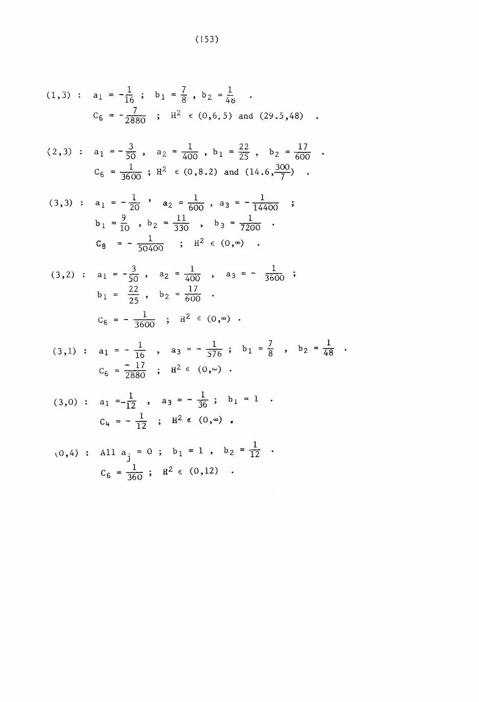
(I53)
(1,3)1
b l7
b 21
al = .16
,8 ,
4t>
C67
H2 (0,6.5) and (29.5,48)= --- . E2880 ,
(2,3) 3 1b l
22b 2
17al =-,- a2 - 400 - = 60050 , , 25 ,
1 H2 E (0,8.2) and300
C6 = . (14.6 '-7-)3600 ,
(3,3) 1 , 1 1al = -- a2 = 600 a3 = -20 14400
b l9
b 211
b 31= - = 330 =10
, , 7200
Ce1
H2 (0,00)= E50400
3 1 1 .(3,2) al = a2 - 400 a3 - 3600 ,50
,
22b 2
17bl = - = 60025
1H2 E (0,00)C6
. .- 3600 ,
1 1 7 b 21
(3,1) al = -- a3 = - -- b l 8 , - 4816 576- 17 H2 E (O,w)C6 = .2880
(3,0)
,,0,45
1 1 b i = 1a3 = - 36.
al =-12 , ,
1 H2 e: (0,00)C4 = -- •12
b 21
All = 0 . b l = 1 =-a. , , 12J
1 H2 E (0,12)C 6 = 360.,
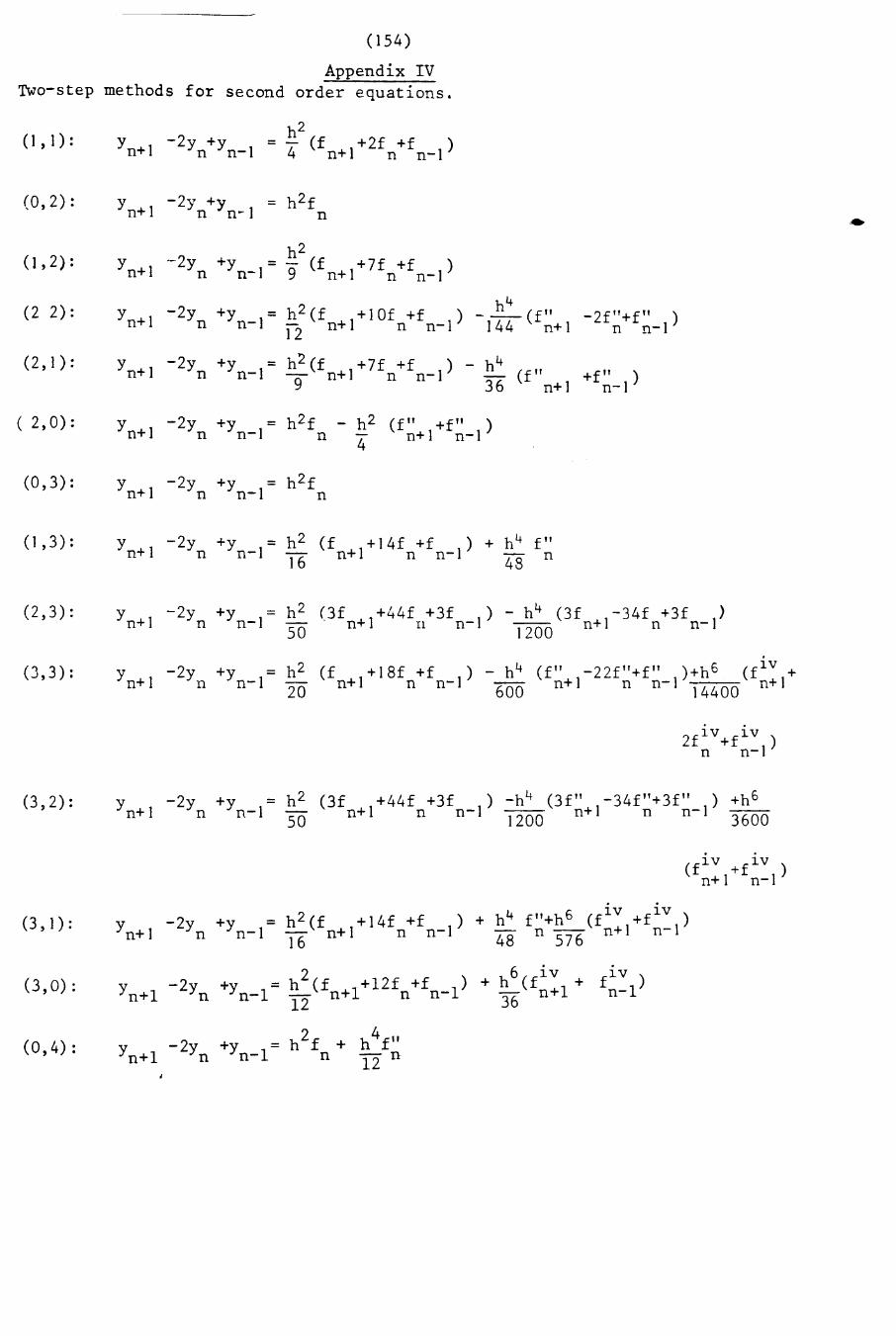
(154)
Appendix IVTwo-step methods for second order equations.
(1,1): h2Yn+1 -2y +y = -4 (f }+2f +f )n n-} n+ n n-}
(0,2):
(1,2):
(2 2):
(2,1):
( 2,0):
(0,3):
(1,3):
(2,3):
(3,3):
(3,2):
(3,1):
(3,0):
(0,4) :
Yn+1-2y +y = h2(f +10f +f ) h
4(f" -2f"+f" )n n-1 12 n+1 n rr-I -i44 n+1 n n-1
Yn+} -2y +y = h2(f +7f +f ) - h4(f " +f" )n n-r l 9 n+1 n n--I
36 n+1 n-1
Yn+1-2y +y = h2f - h2 (f" +f" )n n-1 n
4 n+ I n-1
Yn+1-2y +y = h2f
n n-1 n
Yn+1-2y +y = h 2 (f 1+14f +f I) + h4 f"n n-1 - n+ n n- n16 48
y -2y +y = h 2 (3f 1+44f +3f I) - h4 (3f -34f +3f )n+ I n n-1 50 n+ Il n- 1200 n+ I n rr-J
y -2y +y = h2 (f 1+18f +f I) - h" (f" -22f"+f" )+h 6 (flV +n+1 n n-1 20 n+ n n- 600 n+1 n n-1 14400 n+1
. .2f 1V+f1V )
n n--I
2 +y = h 2 (3f 1+44f +3f I) -h4 (3f" -34f"+3f" ) +h6Yn+1 - Yn n-1 50 n+ n n- 1200 n+l n n-1 3600
. .(f1V +f 1V )
n+ 1 n-l. .
-2y +y = h2(f +14f +f I) + h4 f"+h 6 (f1V +f1V
)Yn+1 n n-1 16 n+1 n n- 48 n 576 n+1 n-1
2 ) + h6(fiv + f1 V )Y -2y +y 1= h (f 1+12f +f -1n+1 n n- 12 n+ n n 36 n+1 n-1
2 +y = h 2f + h4
f IIYn+1 - Yn n-1 n 12 n
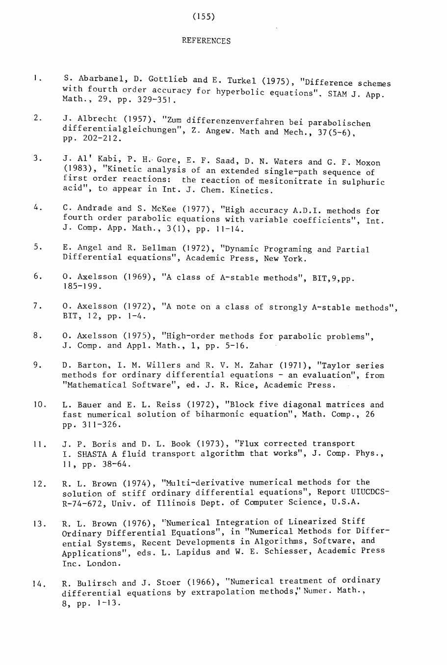
(155)
REFERENCES
I .
2.
3.
S: Abarbanel, D. Gottlieb and E. Turkel (1975), "Difference schemeswlth fourth order accuracy for hyperbolic equations". SIAM J. App.Math., 29~ pp. 329-351. .
J. Albrecht (1957L "Zum differenzenverfahren bei parabolischendifferentialgleichungen", Z. Angew. Math and Mech., 37(5-6),pp. 202-212.
J. AI' Kabi, P. H.· Gore, E. F. Saad, D. N. Waters and G. F. Moxon(~983), "Kinetic ~nalysis of an extended single-path sequence offlrst order reactl0ns: the reaction of mesitonitrate in sulphuric
. d" .aCl ,to appear ln Int. J. Chern. Kinetics.
4. C. Andrade and S. McKee (1977), "High accuracy A.D.I. methods forfourth order parabolic equations with variable coefficients", Int.J. Compo App. Math., 3(1), pp. 11-14.
5. E. Angel and R. Bellman (1972), "Dynamic Programing and PartialDifferential equations", Academic Press, New York.
6. O. Axelsson (1969), "A class of A-stable methods", BIT,9,pp.185-199.
7. O. Axelsson (1972), "A note on a class of strongly A-stable methods",BIT, 12, pp , 1-4 .
8. O. Axelsson (1975), "High-order methods for parabolic problems",J. Compo and Appl. Math., 1, pp. 5-16.
9. D. Barton, I. M. Willers and R. V. M. Zahar (1971), "Taylor seriesmethods for ordinary differential equations - an evaluation", from"Mathematical Software", ed. J. R. Rice, Academic Press.
10. L. Bauer and E. L. Reiss (1972), "Block five diagonal matrices andfast numerical solution of biharmonic equation", Math. Comp., 26pp. 311-326.
11. J. P. Boris and D. L. Book (1973), "Flux corrected transportI. SHASTA A fluid transport algorithm that works", J. Compo Phys.,11, pp. 38-64.
12.
13.
14.
R. L. Brown (1974), "Multi-derivative numerical methods for thesolution of stiff ordinary differential equations", Report UIUCDCSR-74-672, Univ. of Illinois Dept. of Computer Science, U.S.A.
R. L. Brown (1976), "Numer i.caI Integration of Linearized Stif~Ordinary Differential Equations", in "Numerical Methods for Dlfferential Systems, Recent Developments in Algorithms, Softwar:, andApplications", eds. L. Lapidus and W. E. Schiesser, AcademlC PressInc. London.
R. Bulirsch and J. Stoer (1966), "Numerical treatment of ordinarydifferential equations by extrapolation methods;'Numer. Math.,8, pp. 1-13 .
(156)
15. B. L. Buzbee and F. W. Door (1974), "The direct solution of biharmonic equation on rectangular regions and the Poisson equationon irregular regions". SIAM J. Numer. Anal., 11(4). pp. 753-763.
16. B. L. Buzbee. F. W. Door. J. A. George and G. H. Golub (1971)"The direct solution of the discrete Poisson equation on irre~ularregions", SIAM J. Numer. Anal., 8, pp. 722-736.
17. J. R. Cash (1980), "On the integration of stiff system of O.D.Esusing extended backward differentiation formulae", Numer. Math.,34, pp. 235-246.
18. J. R. Cash (1981), "High order P-stable formulae for the numericalintegration of periodic initial value problems", Numer. Math., 37,pp. 355-370.
19. M. M. Chawla (1981), "Two-step fourth order P-stable methods forsecond order differential equations", BIT, 21, pp.190-193.
20. F. H. Chapman (1971), "A-stable Runge-Kutta processes", BIT, 11,pp. 384-388.
21. M. Ciment and S. H. Leventhal (1975), "High order compact implicitschemes for the wane equation", Math. Comp . , 29 (132), pp. 985-994.
22. L. Collatz (1951), "Zur stabilitat des differenzenverfahrens beider stabschwingungsgleichung", Z. Angew. Math and Mech., 31, pp.392-393.
23. S. D. Conte (1957), "A stable implicit finite difference app r ox r-:mat ions to a fourth order parabolic equation", J. Assoc. CompoMach., 4, pp. 202-212.
24. S. D. Conte and W. C. Royster (1956), "Convergence of finitedifference solutions to a solution of the equation of the vibrating rode", Proc. Amer. Math. Soc., 7, pp. 742-749.
25. S. H. Crandall (1954), "Numerical treatment of a fourth orderpartial differential equation", J. Assoc. Compo Mach., 1, pp.111-118.
26. J. Crank and P. Nicolson (1947), "A practical method for numericalevaluation of solutions of partial differential equations of theheat-conduction type", Proc. Cambridge Philos. Soc., 43, pp.50-67.MR 8, 409.
A o27.
28.
29.
C. W. Cryer (1973), "A new class of highly stable methods:stable methods", BIT, 13, pp. 153-159.
G. Dahlquist (1963), "A special stability problem for linearmultistep methods", BIT, 3, pp. 27-43.
G. Dahlquist (1977), "On the relation of G-stab~li~y ~o o~her.stability concepts for linear multistep methods ~ 1n Top1cs 1nNumerical Analysis III, ed. J. J. Miller, Academ1c Press.
30. G. Dahlquist (1978), "Onlinear multistep methodsBIT, 18, pp. 133-136.
accuracy and unconditional stability of. ."for second order different1al equat10ns ,
(157)
31 . J. Douglas, JR. (1956), "The solution of diffusion equation by ahigh order correct difference equation!', J. Math. Phys, 35, pp.145-151, MR 19, 884.
32. E. C. Du Fort and S. P. Frankel (953), "Stability conditions inthe numerical treatment of parabolic partial differential equations ll ,
MTAC, 7, pp. 135-152, MR 15, 474.
33. B. L. Ehle (1968), "High order A-stable methods for the numericalsolution of system of differential equations", BIT, 8, pp. 276-278.
34. B. L. Ehle (1969), "On Pade approximations to the exponentialfunction and A-stable methods for the numerical solution of initialvalue problems", Re. Rept. CSRR 2010. University of Waterloo, Canada.
35. L. W. Ehrlich (1973), "Solving the biharmonic equation in a square:A direct versus a semidirect method", Comm. ACM, 16, pp. 711-714.
36. D. J. Evans (1965), "A stable explicit method for the finite difference solution of fourth order parabolic partial differential equation",Compo J., 8, pp. 280-287.
37.
38.
39.
40.
41.
42.
43.
44.
45.
46.
G. Fairweather (1978), "A note on the efficient implementation ofcertain Pade methods for linear parabolic problems", BIT, 18, pp.106-109.
G. Fairweather, A. R. Gourlay and A. R. Mitchell (1967), "Some highaccuracy difference schemes with a splitting operator for equationsof parabolic and elliptic type", Numer. Math., 10, pp. 56-66.
G. Fairweather and A. R. Gourlay (1967), "Some stable differenceapproximations to a fourth order parabolic partial differentialequation", Math. Comp , , 21, pp. 1-11.
I. Fried (1979), "Numerical Solution of Differential Equations",Academic Press, London.
W. Gautschi (1961), "Numerical integration of ordinary differentialequations based on trigonometric polynomial", Numer. Math, 3,381-397.
C. w. Gear (1971), "Numerical Ini tial Value Problems in OrdinaryDifferential Equations", Prentice Hall, Englewood Cliffs, NewJersey.
M. Goldberg and E. Tadmore (1978), "Scheme-indepen~en~ ~t~bilitycriteria for difference approximations of hyperbo11c 1n1t1alboundary value problems.I", Math. Comp , , 32, pp. 1097-1107.
D. J. Gorman (1975), "Free Vibration Analysis of Beams and Shafts",
John Wiley, New York.
A. R. Gourlay and J. LI. Morris (1968), "Finite difference methodsfor nonlinear hyperbolic systems", Math. Comp., 22, pp. 28-39.
A. R. Gourlay and J. Ll. Morris (1980), "The extrapolation of first. I . II",order methods for parabolic partial different1a equat10ns
SIAM J. Numer. Anal., 17(5), pp. 641-655.
47.
48.
49.
(158)
A. R. Gourlay and J. LI. Morris (1981), "Linear Combinat'; of. I" .LonsGeneralized Crank-N~co son schemes, lMA J. Numer. Anal., I,
347-357. pp.
P. R. Graves-Morris. (ed ) (1973), lrpade Approximants and theirApplications", Academic Press, London.
B. ?ustafsso~ (19~5~,."The convergence rate for difference approxima t i ons to mi.xed t.m, t~al-boundary value problems", Maths. Comp.,29, pp. 396-406.
50. B. Gustafsson, H.-O. Kreiss and A. Sundstrom (1972), "Stabilitytheory of differ~nce approximations for mixed initial-boundaryvalue problems. II", Maths. Comp., 26, pp. 649-686.
of low
51 .
52.
53.
54.
55.
56.
57.
58.
59.
60.
61.
62.
63.
A. Hadjidimos (1971), "The numerical solution of model problembiharmonic equation by using extrapolated alternating directionimplicit method", Ibid., 17, pp.301-317.
E. Eairer (1979), "Unconditionally stable methods for second orderdifferential equations", Numer. Math., pp. 373-379.
C. A. Hall and T. A. Porsching (1980), "Pade approximants,fractional step methods and Navier-Stokes discretizations", SIAMJ. Numer. Anal., 17(6), pp. 840-851.
G. Hall and J. M. \-Jatt. (eds) (I 976), "Modern Numerical MethodsFor Ordinary Differential Equations", Clarendon Press, Oxford.
P. Henrici (1962), "Dicrete Variable Methods ~n Ordinary Differential Equations", John Wiley and sons.
R. S. Hirsch and D. H. Rudy (1974), "The role of diagonal dominance and the cell Reynolds number in implicit difference methodsfor fluid mechanics problems", J. Compo Phys, 16, pp. 304-310.
M. K. Jain, R. K. Jain, U. A. Krishnaiah (1979), "P-stable methodsfor periodic initial value problems of second order differentialequations", BIT, 19, pp. 347-355.
A. Q. M. Khaliq and E. H. Twizell (1982), "The extrapolation ofstable finite difference schemes for first order hyperbolicequations", Intern. J. Computer Math., II, pp. 155-167.
H. -0. Kreiss and J. Oliger (1972), "Comparison of accurate methodsfor the integration of hyperbolic equations", Tellus, 24, pp.199-215.
J. D. Lambert (1973), "Computational Methods in Ordinary DifferentialEquations", John Wiley, Chichester.
J. D. Lambert (1980), "Stiffness", in "Computational Techniques forOrdinary Differential Equations" (eds. I. Gladwell and D. K. Sayers),Academic Press, London.
J. D. Lambert and A. R. Mitchell (1962), "On the solution ofy' = f(x,y) by a class of high accuracy difference formulaeorder", Z. Angew. Math. Phys, 13, pp. 223-232.
J. D. Lambert and I. A. Watson (1976), "Symmetric multistep methodsfor periodic initial value problems", J. Inst. Maths. Applies., 18,pp. 189-202.
--------_./( 159)
64. J. D. Lawson and B. L. Ehle (1970) , "Asymptotic error estimationfor one-step methods based on quadrature ll
, Aeq. Math, 5, pp.236-246.
65. J. D. Lawson and J. t.i . Morris (1978), "The extrapolation of firstorder methods for parabolic partial differential equations I", SIAMJ. Numer. Anal., 15(6), pp. ]2]2-]224.
66. J. D. Lawson and D. Swayne (1976), "A simple efficient algorithmfor the solution of heat conduction problems", Proceedsings, SixthManitoba Conference on Numerical Mathematics, pp. 239-250.
67. M. Lees (]960), "A priori estimates for the solution of differenceapproximations to parabolic partial differential equations", DukeMath. J., 27, pp. 297-312, MR22, 12725.
68. M. Lees (196]), "Alternating direction and semi-explicit differencemethods for parabolic partial differential equations", Numer. Math,3, pp. 24-47, MR 27, 5376.
69. B. Lindberg (197]), "On smoothing and extrapolation for the trapezoidal rule", BIT, ]], pp. 29-52.
70. W. Liniger and R. A. Willoughby (1967), "Efficient numerical integration methods for stiff systems of differential equa t i.ons!", IBMResearch Report RC-]970, Thomas J. Watson Research Centre, YorktownHeights, N.Y.
71 . W. E. Milne (1949), "A note on the numerical integration of differential equations", J. Res.Nat. Bur. Standards., 43, pp. 537-542.
72. A. R. Mitchell (1969), "Computational Methods in Partial DifferentialEquations", John Wiley, Chichester.
73. A. R. Mitchell and D. F. Griffiths (1980), "The Finite DifferenceMethod in Partial Differential Equations", John Wiley, Chichester.
74. K. W. Morton (1980), "Stability of finite difference approximationsto a diffusion-convection equation", Int. J. num. Meth. Engng, ]2,pp.899-9]6.
of theMath.
75.
76.
77.
78.
79.
80.
S. P. Norsett (1975), "Numerical Solution of Ordinary DifferentialEquations", Ph. D. Thesis, University of Dundee, U.K.
S. P. Norsett (1978), "Restricted Pad~ approximations to the exponential function", SIAM J. Numer. Anal., 15, pp. 1008-]029.
N. Obrechkoff (]942), "Sur les quadrature mecaniques", SpisanicBulgar. Akad. Nauk., 65, pp. 191-289 (in Bulgarian, French summary),(Reviewed in Math. Rev., 10, p.70.)
C. G. O'Brien, M. A. Hyman and S. Kap l an (]951),."A ~tudYnumerical solution of partial differentlal equatlons , J.Phys, 29, pp. 223-25].
01 ' (1974) "Fourth order difference methods for the initialJ. r.ger , . "M h C 28boundary-value problem for hyperbolic equatlons, at. omp., ,
pp. ]5-25.
M. H. Pad~ (1892), "Sur la representation approch~e d'une fonction
81.
82.
83.
84.
85.
86.
87 .
88.
89.
90.
91.
92.
93.
94.
95.
(160)
par des fractions rationelles, Ann. de l'Ecole Normale Sup~' "erleure ,Vol. 9 (Suppl.).
D. W. Peaceman and H. H. Rachford (1955), "The numerical so lu t if . 11""" 0 u r ono parabollc and e lptlC dlfferential equations" J Soc I d,. . n ust.
Appl. Math., 3, pp. 28-4].
H. S. Price, R. S. Varga and J. E. Warren (1966), "Application ofoscillation matrices to diffusion - convection equation", J. Math.Phys., 45, pp. 301-3]1.
R. D. Richtmyer (957), "Difference methods for initial valueproblems, Interscience Tracts in Pure and Applied Mathematics",Tract 4, Interscience, New York, MR 20, 438.
R. D. Richtmyer (1963), "A survey of finite difference methods fornonsteady fluid dynamics", NCAR Research Tech. notes 63-2.
R. D. Richtmyer and K. W. Morton (1967), "Difference Methods forInitial-Value Problems", John Wiley, New York.
H. H. Rosenbrock (1963), "Some general implicit processes for thenumerical solution of differential equations", Compo J, 5, pp.329-330.
L. F. Shampine and M. K. Gordon (1973), "Computer Solution ofOrdinary Differential Equations", W. H. Freeman and Company, SanFrancisco.
G. D. Smith (1978), "Numerical Solution of Partial DifferentialEquations: Finite Difference Methods", 2nd edn, Clarendon Press,Oxford.
I. M. Smith, J. L. Siemieniuch and I. Gladwell (1973), "A com-parison of old and new methods for large systems of ordinary differential equations arising from parabolic partial differential equations",Numerical Analysis Research Report no. 13, Mathematics Department,University of Manchester, Manchester, England.
P. Smith and E. H. Twizell (1982), "The extrapolation of Pad eapproximants in the closed-loop simulation of human thermoregulation",Appl. Math. Modelling, 6, pp. 81-91.
E. Stiefel and D. G. Bettis (1969), "Stabilization of Cowell's methods",Numer. Math., 13, pp. 154-175.
G. J. Tee (1975), "! novel finite-difference approximation to thebiharmonic operator", Compo J, 6, pp . 177-192.
C. E. Thompson (1968), "Solution of linear differential equations",Compo J, 10, pp. 417-418.
E. H. Twizell (1979), "An explicit difference method for the waveequation with extended stability range",BIT, 19, pp. 378-383,
H T · 11 (1981) "The numerical solution of the wave equationE. . wi.ze , f h 'at the first time step", BruneI University Department 0 Mat ematlcsTechnical Report, TR/13/81.
( 161)
96. E. H. Twizell and A. Q. M. Khaliq (1981), "One step multiderivative methods for first order ordinary differential equations",BIT, 21, pp. 518-527.
97. E. H. Twizell and P. S. Smith (1981), "A numerical study of heatflow in elliptic cylinder with interior derivative boundary conditions", BruneI University Department of Nathematics TechnicalReport, TR/l1/81.
98. E. H. Twizell and P. S. Smith (1982), "Numerical modelling of heatflow in the human torso I: finite difference methods", in J.Caldwell and A..0. Moscardini (eds.), "Numerical Modelling inDiffusion-Convection", Pentech Press, Plymouth, pp. 165-189.
99. R. S. Varga (1961), "On high order stable implicit methods forsolving parabolic partial differential equations", J. Math. Phys,40, pp. 220-231.
100. R. S. Varga (1962), "Matrix Iterative Analysis", Prentice Hall,Englewood Cliffs, N.J.
101 . IV. L. Wood and R. W. Lewis (I 975), "A Comparison of Time-MarchingSchemes for the Transient Heat Conduction Equation", Internat. J.Numer. Method. Engrg., 9, pp. 679-689.