Numerical Method for Computing Numerical Method for Computing Ground States of Spin-1 Ground States of Spin-1

Bose-Einstein CondensatesBose-Einstein Condensates

Fong Yin LimFong Yin Lim

Department of MathematicsDepartment of Mathematicsandand

Center for Computational Science & EngineeringCenter for Computational Science & EngineeringNational University of SingaporeNational University of SingaporeEmail: Email: fongyin.lim@nus.edu.sgfongyin.lim@nus.edu.sg

Collaborators: Weizhu Bao (National University of Singapore)Collaborators: Weizhu Bao (National University of Singapore) I-Liang Chern (National Taiwan University)I-Liang Chern (National Taiwan University)

OutlineOutline

Introduction Introduction

The Gross-Pitaevskii equation The Gross-Pitaevskii equation

Numerical method for single component BEC Numerical method for single component BEC ground stateground state

Gradient flow with discrete normalizationGradient flow with discrete normalizationBackward Euler sine-pseudospectral methodBackward Euler sine-pseudospectral method

Spin-1 BEC and the coupled Gross-Pitaevskii Spin-1 BEC and the coupled Gross-Pitaevskii equationsequations

Numerical method for spin-1 condensate ground Numerical method for spin-1 condensate ground statestate

ConclusionsConclusions

Single Component BECSingle Component BEC

Hyperfine spin Hyperfine spin FF = = I I + + SS

2F+12F+1 hyperfine components: hyperfine components: mmFF = -F, -F+1, …., F-1, F = -F, -F+1, …., F-1, F

Experience different potentials under external magnetic Experience different potentials under external magnetic fieldfieldEarlier BEC experiments: Cooling of magnetically trapped Earlier BEC experiments: Cooling of magnetically trapped atomic vapor to nanokelvins temperature atomic vapor to nanokelvins temperature single single component BECcomponent BEC

ETH (02’,87Rb)

Spinor BECSpinor BEC

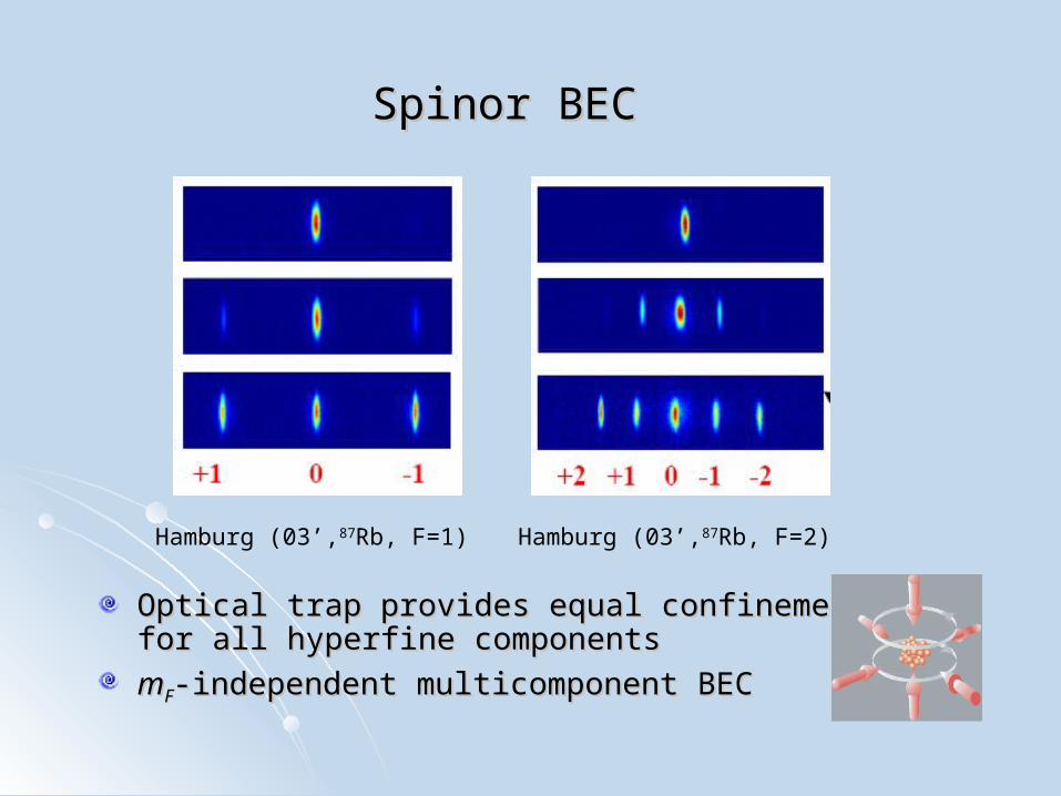
Optical trap provides equal confinement for all Optical trap provides equal confinement for all hyperfine componentshyperfine components

mmFF-independent multicomponent BEC-independent multicomponent BEC

Hamburg (03’,87Rb, F=1) Hamburg (03’,87Rb, F=2)

Gross-Pitaevskii EquationGross-Pitaevskii Equation

GPE describes BEC at GPE describes BEC at T <<TT <<Tcc

Non-condensate fraction can be neglectedNon-condensate fraction can be neglectedInteraction between particles is treated by mean field Interaction between particles is treated by mean field approximationapproximation

where interparticle mean-field interactionwhere interparticle mean-field interaction

Number densityNumber density

txtxnctxxVtxm

txt

i ,,,,2

, 02

2

Nxdtx 2

,

2,, txtxn

mac s /4 20

Dimensionless GPEDimensionless GPE

Non-dimensionalization of GPENon-dimensionalization of GPE

Conservation of total number of particlesConservation of total number of particles

Conservation of energyConservation of energy

Time-independent GPETime-independent GPE

12 N

22 )(2

1

xVt

i

xdtxtxxVtxtE 422

,2

,,2

1

)()()()()(2

1)(

22 xxxxVxx

tiextx )(),(

BEC Ground StateBEC Ground State

Boundary eigenvalue methodBoundary eigenvalue method Runge-Kutta space-marchingRunge-Kutta space-marching (Edward & Burnett, (Edward & Burnett, PRAPRA, 95’), 95’)

(Adhikari, (Adhikari, Phys. Lett. APhys. Lett. A, 00’), 00’) Variational methodVariational method

Direct minimization of energy functional with FEM approachDirect minimization of energy functional with FEM approach (Bao & Tang, (Bao & Tang, JCPJCP, 02’), 02’)

Nonlinear algebraic eigenvalue problem approachNonlinear algebraic eigenvalue problem approachGauss-Seidel type iterationGauss-Seidel type iteration (Chang et. al., (Chang et. al., JCPJCP, 05’), 05’)

Continuation methodContinuation method (Chang et. al., (Chang et. al., JCPJCP, 05’), 05’) (Chien et. al., (Chien et. al., SIAM J. SIAM J.

Sci. ComputSci. Comput., 07’)., 07’)

Imaginary time methodImaginary time methodExplicit imaginary time algorithm via Visscher schemeExplicit imaginary time algorithm via Visscher scheme (Chiofalo et. al., (Chiofalo et. al., PREPRE, 00’), 00’)

Backward Euler finite difference (BEFD) and time-splitting Backward Euler finite difference (BEFD) and time-splitting sine-pseudospectral methodsine-pseudospectral method (TSSP) (TSSP) (Bao & Du, (Bao & Du, SIAM J. Sci. ComputSIAM J. Sci. Comput., 03’)., 03’)

--

Imaginary Time MethodImaginary Time Method

Replace Replace in the time-dependent GPE in the time-dependent GPE (imaginary time method) and form gradient flow with (imaginary time method) and form gradient flow with discrete normalization (GFDN) in each time intervaldiscrete normalization (GFDN) in each time interval

BEFD – BEFD – implicit, unconditionally stable, energy diminishing, second order accuracy in space second order accuracy in space

TSSP – explicit, conditionally stable, TSSP – explicit, conditionally stable, spectral accuracy in space

1

22 ,)(2

1

nndd tttxVt

itt

),(

),(),(

1

11

n

nn

tx

txtx

--

Discretization SchemeDiscretization Scheme

The problem is truncated into bounded domain with The problem is truncated into bounded domain with zero boundary conditionszero boundary conditions

Backward Euler sine-pseudospectral method (BESP)Backward Euler sine-pseudospectral method (BESP)( Bao, Chern ( Bao, Chern

& Lim, & Lim, JCPJCP, 06’), 06’)

Backward Euler scheme is applied, except the non-Backward Euler scheme is applied, except the non-linear interaction termlinear interaction term

Sine-pseudospectral method for discretization in spaceSine-pseudospectral method for discretization in space

Consider 1D gradient flow in Consider 1D gradient flow in 1 nn ttt

1,,2,1,)(2

1 *2***

MjxVD

t jnjjjxx

sxx

njj

j

0**0 M

Mjjnj ,,1,0,

*

*1

Backward Euler Sine-pseudospectral Backward Euler Sine-pseudospectral Method (BESP)Method (BESP)

At every time step, a linear system is solved iterativelyAt every time step, a linear system is solved iteratively

Differential operator of the second order spatial derivative Differential operator of the second order spatial derivative of vector of vector U=(UU=(U00, U, U11, …, U, …, UMM))TT

; ; UU satisfying satisfying UU00 = U = UMM = 0 = 0

The sine transform coefficientsThe sine transform coefficients

1

1

2 1,,2,1,)(sin)ˆ(2 M

ljlllxx

sxx MjaxU

MUD

j

1

1

1,,2,1,,)(sin)ˆ(M

jljljl Ml

ab

laxUU

mj

njjxx

msxx

nj

m

xVDt j

*,21*,1*,

)(2

1

Backward Euler Sine-pseudospectral Backward Euler Sine-pseudospectral Method (BESP)Method (BESP)

A stabilization parameter A stabilization parameter is introduced to ensure the is introduced to ensure the convergence of the numerical schemeconvergence of the numerical scheme

Discretized gradient flow in position spaceDiscretized gradient flow in position space

Discretized gradient flow in phase spaceDiscretized gradient flow in phase space

mj

njj

mjxx

msxx

nj

m

xVDt j

*,21*,1*,1*,

)(2

1

Mjnjj ,,1,0,0*,

MjxVG mj

njj

mj ,,1,0,)( *,2

1,,2,1,)ˆ()ˆ(22

2)ˆ(

21*,

MlGt

t lm

ln

ll

m

Backward Euler Sine-pseudospectral Backward Euler Sine-pseudospectral Method (BESP)Method (BESP)

Stabilization parameterStabilization parameter

guarantees the convergence of the iterative method guarantees the convergence of the iterative method and gives the optimal convergence rateand gives the optimal convergence rateBESP is spectrally accurate in space and is BESP is spectrally accurate in space and is unconditionally stable, thereby allows larger mesh size unconditionally stable, thereby allows larger mesh size and larger time-step to be usedand larger time-step to be used

minmax2

1bb

2

11min

2

11max )(min,)(max n

jjMj

njj

MjxVbxVb

BEC in 1D PotentialsBEC in 1D Potentials

-16 -8 0 8 160

0.1

0.2

0.3

0.4

g(x)

-16 -8 0 8 160

35

70

105

140

V(x

)

x

400,2

)(2

xxV

-16 -8 0 8 160

0.1

0.2

0.3

0.4

g(x)

-16 -8 0 8 160

35

70

105

140

V(x

)

x

250,4

sin252

)( 22

xx

xV

BEC in 1D Optical LatticeBEC in 1D Optical Lattice

Comparison of spatial accuracy of BESP and backward-Euler Comparison of spatial accuracy of BESP and backward-Euler finite difference (BEFD)finite difference (BEFD)

BEC in 3D Optical LatticeBEC in 3D Optical Lattice

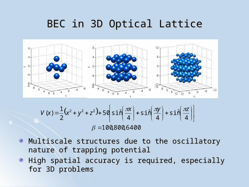
Multiscale structures due to the oscillatory nature of trapping Multiscale structures due to the oscillatory nature of trapping potentialpotential

High spatial accuracy is required, especially for 3D problemsHigh spatial accuracy is required, especially for 3D problems

6400,800,100

4sin

4sin

4sin50

2

1)( 222222

zyxzyxxV

Spin-1 BECSpin-1 BEC

3 hyperfine components: 3 hyperfine components: mmFF = -1, 0 ,1 = -1, 0 ,1

Coupled Gross-Pitaevskii equations (CGPE)Coupled Gross-Pitaevskii equations (CGPE)

ββnn -- -- spin-independent mean-field interaction spin-independent mean-field interaction

ββss -- s -- spin-exchange interactionpin-exchange interaction

Number densityNumber density nnnnn ii 0

2,

200

2

00020

200

2

)()(2

1

2)()(2

1

)()(2

1

ssn

ssn

ssn

nnnnxVt

i

nnnxVt

i

nnnnxVt

i

Spin-1 BECSpin-1 BEC

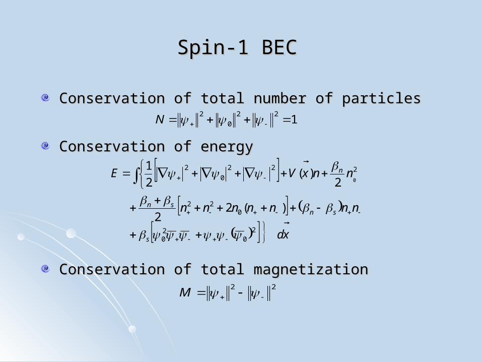
Conservation of total number of particlesConservation of total number of particles

Conservation of energyConservation of energy

Conservation of total magnetizationConservation of total magnetization

122

0

2 N

22

M

xd

nnnnnnn

nnxVE

s

snsn

n

20

20

022

222

0

2

)(22

2)(

2

10

Spin-1 BECSpin-1 BEC

Time-independent CGPETime-independent CGPE

Chemical potentialsChemical potentials

Lagrange multipliers, Lagrange multipliers, µ µ and and λλ,, are introduced to the are introduced to the free energy to satisfy the constraints N and Mfree energy to satisfy the constraints N and M

200

2

0002

00

200

2

)()(2

1

2)()(2

1

)()(2

1

ssn

ssn

ssn

nnnnxV

nnnxV

nnnnxV

,, 0

tiii

iextx )(),(

Spin-1 BEC Ground StateSpin-1 BEC Ground State

Imaginary time propagation of CGPE with initial Imaginary time propagation of CGPE with initial complex Gaussian profiles with constant speedcomplex Gaussian profiles with constant speed

Continuous normalized gradient flow (CNGF)Continuous normalized gradient flow (CNGF)

-- -- -- N-- N and and MM conserved, energy diminishing conserved, energy diminishing-- Involve -- Involve and implicitlyand implicitly

200

2

00020

200

2

)()()(2

1

2)()(2

1

)()()(2

1

ssn

ssn

ssn

nnnnxVt

nnnxVt

nnnnxVt

(Zhang, Yi & You, (Zhang, Yi & You, PRA,PRA, 02’) 02’)

(Bao & Wang, (Bao & Wang, SIAM J. Numer. AnalSIAM J. Numer. Anal., 07’)., 07’))(),( tt

Normalization ConditionsNormalization Conditions

Numerical approach with GFDN by introducing third Numerical approach with GFDN by introducing third normalization conditionnormalization condition

Time-splitting scheme to CNGF in Time-splitting scheme to CNGF in 1.1. Gradient flowGradient flow

2.2. Normalization/ ProjectionNormalization/ Projection

200

2

00020

200

2

)()(2

1

2)()(2

1

)()(2

1

ssn

ssn

ssn

nnnnxVt

nnnxVt

nnnnxVt

)(,,)( 00

ttt

1 nn ttt

Normalization ConditionsNormalization Conditions

Normalization stepNormalization step

Third normalization conditionThird normalization condition

Normalization constantsNormalization constants

*)(

*0

*)(

0

t

t

t

e

e

e

20

2

1

2*

2*0

22

1

2*

2*0

2

2

1

4*0

22*2*22*0

2

0

2

1,

2

1

)1(4

1

00

MM

MM

M

*

*00

*

0

Discretization SchemeDiscretization Scheme

Backward-forward Euler sine-pseudospectral method Backward-forward Euler sine-pseudospectral method (BFSP) (BFSP)

Backward Euler scheme for the Laplacian; forward Euler Backward Euler scheme for the Laplacian; forward Euler scheme for other termsscheme for other terms

Sine-pseudospectral method for discretization in spaceSine-pseudospectral method for discretization in space

1D gradient flow for 1D gradient flow for mmFF = +1 = +1

ExplicitExplicit

Computationally efficientComputationally efficient

nj

njs

nj

nj

nj

njs

njnj

jxx

sxx

njj

nnnnxV

Dt j

,

2

,0,,,0,

*,

*,*

,

)(

2

1

8787Rb in 1D harmonic potentialRb in 1D harmonic potential

Repulsive and ferromagnetic interaction (Repulsive and ferromagnetic interaction (ββnn >0 >0 , , ββss < 0) < 0)

Initial conditionInitial condition

2/4/1

02/4/1

00

2/4/1

0 222 )1(5.0,,

)1(5.0 xxx eM

eeM

8787Rb in 1D harmonic potentialRb in 1D harmonic potential

-16 -8 0 8 160

0.05

0.1

0.15

0.2

0.25

-16 -8 0 8 160

30

60

90

120

150

x

M=0.2

42

10,2

)( Nx

xV

-16 -8 0 8 160

0.05

0.1

0.15

0.2

0.25M=0.7

-16 -8 0 8 160

30

60

90

120

150

x

V(x

)

Repulsive and ferromagnetic interaction (Repulsive and ferromagnetic interaction (ββnn >0 >0 , , ββss < 0) < 0)

-16 -8 0 8 160

0.05

0.1

0.15

0.2

0.25

x

(x)

-16 -8 0 8 160

30

60

90

120

150M=0

|+|

|0|

|-|

2323Na in 1D harmonic potentialNa in 1D harmonic potential

-12 -6 0 6 120

0.1

0.2

0.3

-12 -6 0 6 120

30

60

90

x

M=0.2

42

10,2

)( Nx

xV

-12 -6 0 6 120

0.1

0.2

0.3

x-12 -6 0 6 12

0

30

60

90

V(x

)

M=0.7

Repulsive and antiferromagnetic interaction (Repulsive and antiferromagnetic interaction (ββnn >0 >0 , , ββss > 0) > 0)

Initial conditionInitial condition

-12 -6 0 6 120

0.1

0.2

0.3

x

(x)

-12 -6 0 6 120

30

60

90M=0

|+|

|0|

|-|

2/4/1

02/4/1

00

2/4/1

0 222 )1(5.0,,

)1(5.0 xxx eM

eeM

8787Rb in 3D optical latticeRb in 3D optical lattice

)

2(sin)

2(sin)

2(sin100

2

1)( 222222 zyx

zyxxV

5.0,104 MN

2323Na in 3D optical latticeNa in 3D optical lattice

)

2(sin)

2(sin)

2(sin100

2

1)( 222222 zyx

zyxxV

5.0,104 MN

Relative PopulationsRelative Populations

0 0.2 0.4 0.6 0.8 10

0.2

0.4

0.6

0.8

1

M

||+||2

||0||2

||-||2

0 0.2 0.4 0.6 0.8 10

0.2

0.4

0.6

0.8

1

M

Relative populations of each componentRelative populations of each component

Same diagrams are obtained for all kind of trapping potential Same diagrams are obtained for all kind of trapping potential in the absence of magnetic fieldin the absence of magnetic field

ββss < 0 ( < 0 (8787Rb)Rb) ββss > 0 ( > 0 (2323Na)Na)

Chemical PotentialsChemical Potentials

Weighted errorWeighted error

Minimize Minimize ee with respect to with respect to µµ and and λλ

2220

2

022

e

dxnnnnnVx

dxnnnnVx

dxnnnnnVx

ssn

ssn

ssn

200

2

2

200

2

02

0

0

200

2

2

)(2

11

2)(2

11

)(2

11

222222

22

,M

AMB

M

BMA

222

0

2

0

2, BA

Spin-1 BEC in 1D Harmonic PotentialSpin-1 BEC in 1D Harmonic Potential

8787Rb (N=10Rb (N=1044))• E, µ are E, µ are

independent of Mindependent of M• λλ = 0 for all M = 0 for all M

(You et. al., (You et. al., PRAPRA, 02’), 02’)

2323Na (N=10Na (N=1044))

0 0.2 0.4 0.6 0.8 115.2

15.4

15.6

E

0 0.2 0.4 0.6 0.8 1

25.2

25.3

25.4

0 0.2 0.4 0.6 0.8 10

0.4

0.8

M

Spin-1 BEC in Magnetic FieldSpin-1 BEC in Magnetic Field

Spin-1 BEC subject to external magnetic field Spin-1 BEC subject to external magnetic field

Straightforward to include magnetic field in the Straightforward to include magnetic field in the numerical schemenumerical scheme

Stability??Stability??

200

2

000020

200

2

)()()(2

1

2)()()(2

1

)()()(2

1

ssn

ssn

ssn

nnnnxExVt

i

nnnxExVt

i

nnnnxExVt

i

)(xB

ConclusionsConclusions

Spectrally accurate and unconditionally stable method Spectrally accurate and unconditionally stable method for single component BEC ground state computationfor single component BEC ground state computation

Extension of normalized gradient flow and sine-Extension of normalized gradient flow and sine-pseudospectal method to spin-1 condensatepseudospectal method to spin-1 condensate

Introduction of the third normalization condition in Introduction of the third normalization condition in addition to the existing conservation of N and Maddition to the existing conservation of N and M

Future works:Future works:-- -- Extension of the method to spinor condensates with Extension of the method to spinor condensates with higher spin degrees of freedomhigher spin degrees of freedom---- Finite temperature effectFinite temperature effect