numerical mathematics & computing 6th · pdf filenumerical mathematics & computing 6th...
TRANSCRIPT

NUMERICAL MATHEMATICS & COMPUTING6th Edition
Ward Cheney/David Kincaid c©
UT Austin
Engage Learning: Thomson-Brooks/Colewww.engage.com
www.ma.utexas.edu/CNA/NMC6
September 1, 2011
Ward Cheney/David Kincaid c© (UT Austin[10pt] Engage Learning: Thomson-Brooks/Cole www.engage.com[10pt] www.ma.utexas.edu/CNA/NMC6)NUMERICAL MATHEMATICS & COMPUTING 6th EditionSeptember 1, 2011 1 / 42

1.1 Mathematical Preliminaries
Use the Taylor series for the natural logarithm
ln(1 + x) = x − x2
2+
x3
3− x4
4+ · · ·
With x = 1
ln 2 = 1− 1
2+
1
3− 1
4+
1
5− 1
6+
1
7− 1
8+ · · ·
Add the eight terms shown
ln 2 ≈ 0.63452 (poor approx.)
ln 2 = 0.69315. . . . (exact value)
Ward Cheney/David Kincaid c© (UT Austin[10pt] Engage Learning: Thomson-Brooks/Cole www.engage.com[10pt] www.ma.utexas.edu/CNA/NMC6)NUMERICAL MATHEMATICS & COMPUTING 6th EditionSeptember 1, 2011 2 / 42
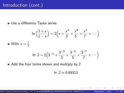
Introduction (cont.)
Use a difference Taylor series
ln(1 + x
1− x
)= 2(x +
x3
3+
x5
5+
x7
7+ · · ·
)With x = 1
3
ln 2 = 2(
3−1 +3−3
3+
3−5
5+
3−7
7+ · · ·
)Add the four terms shown and multiply by 2
ln 2 ≈ 0.69313
Ward Cheney/David Kincaid c© (UT Austin[10pt] Engage Learning: Thomson-Brooks/Cole www.engage.com[10pt] www.ma.utexas.edu/CNA/NMC6)NUMERICAL MATHEMATICS & COMPUTING 6th EditionSeptember 1, 2011 3 / 42

Introduction (cont.)
Rule
Rapid convergence of a Taylor series can be expected near the point ofexpansion, but not at remote points!
ln(1 + x
1− x
)at x = 1
3 is near the point of expansion.
We’re exploiting a more rapidly convergent series!
Taylor series and Taylor’s Theorem are two ubiquitous features inmuch of numerical methods!
Significant digits are digits beginning with the leftmost nonzerodigit and ending with the rightmost correct digit, including final zerosthat are exact.
Ward Cheney/David Kincaid c© (UT Austin[10pt] Engage Learning: Thomson-Brooks/Cole www.engage.com[10pt] www.ma.utexas.edu/CNA/NMC6)NUMERICAL MATHEMATICS & COMPUTING 6th EditionSeptember 1, 2011 4 / 42

Preliminary Mathmatics
Our objectives is to help the student in understanding some of themany methods for solving scientific problems using computers.
We intentionally limit ourselves to the typical problems that arise inscience, engineering, and technology.
We consider problems after they have been cast into certain standardmathematical forms.
You are asked to accept on faith the assertion that the chosen topicsare indeed important ones in scientific computing!
Numerical computations are almost invariably contaminated byerrors, and it is important to understand the source, propagation,magnitude, and rate of growth of these errors.
Ward Cheney/David Kincaid c© (UT Austin[10pt] Engage Learning: Thomson-Brooks/Cole www.engage.com[10pt] www.ma.utexas.edu/CNA/NMC6)NUMERICAL MATHEMATICS & COMPUTING 6th EditionSeptember 1, 2011 5 / 42

Preliminary Mathmatics (cont.)
Numerical methods that provide approximations and error estimatesare more valuable than those that provide only approximate answers.
While we cannot help, but be impressed by the speed and accuracy ofthe modern computer, we should temper our admiration withgenerous measures of skepticism.
Never in the history of mankind has it been possible to produceso many wrong answers so quickly!
One of our goals is to help the studentr arrive at a state ofskepticism, armed with methods for detecting, estimating, andcontrolling errors.
Ward Cheney/David Kincaid c© (UT Austin[10pt] Engage Learning: Thomson-Brooks/Cole www.engage.com[10pt] www.ma.utexas.edu/CNA/NMC6)NUMERICAL MATHEMATICS & COMPUTING 6th EditionSeptember 1, 2011 6 / 42

Example 1 (Significant Digits of Precision)
Example
Using a laser tool, a technician cuts a 2-meter by 3-meter rectangularsheet of metal into two equal triangular pieces.
What is the diagonal measurement of each triangle?
Can these pieces be slightly modified so the diagonals are exactly 3.6?
Ward Cheney/David Kincaid c© (UT Austin[10pt] Engage Learning: Thomson-Brooks/Cole www.engage.com[10pt] www.ma.utexas.edu/CNA/NMC6)NUMERICAL MATHEMATICS & COMPUTING 6th EditionSeptember 1, 2011 7 / 42

Example 1 (cont.)
Since the piece is rectangular, use the Pythagorean Theorem
22 + 32 = d2
where d is the diagonal.
So it follows that
d =√
4 + 9 =√
13 = 3.60555 1275
This last number is obtained by using a hand-held calculator.
The accuracy of d can be verified by computing
(3.60555 1275) ∗ (3.60555 1275) = 13
Is this value for the diagonal, d , to be taken seriously?
Ward Cheney/David Kincaid c© (UT Austin[10pt] Engage Learning: Thomson-Brooks/Cole www.engage.com[10pt] www.ma.utexas.edu/CNA/NMC6)NUMERICAL MATHEMATICS & COMPUTING 6th EditionSeptember 1, 2011 8 / 42

Example 1 (cont.)
Certainly not!
The given dimensions of the rectangle cannot be expected to beprecisely 2 and 3.
If the dimensions are accurate to one millimeter, the dimensions maybe as large as 2.001 and 3.001.
Using the Pythagorean Theorem, the diagonal may be as large as
d =√
2.0012 + 3.0012 =√
4.00400 1 + 9.00600 1
=√
13.01002 ≈ 3.6069
Similar reasoning indicates that d may be as small as 3.6042.
These are both worst cases.
3.6042 ≤ d ≤ 3.6069
No greater accuracy can be claimed for the diagonal d!
Ward Cheney/David Kincaid c© (UT Austin[10pt] Engage Learning: Thomson-Brooks/Cole www.engage.com[10pt] www.ma.utexas.edu/CNA/NMC6)NUMERICAL MATHEMATICS & COMPUTING 6th EditionSeptember 1, 2011 9 / 42

Example 1 (cont.)
If we want the diagonal to be exactly 3.6, we require
(3− c)2 + (2− c)2 = 3.62
reducing each side by the same amount (for simplicity).
This leads toc2 − 5c + 0.02 = 0
Using the quadratic formula, we obtain the smaller root
c = 2.5−√
6.23 ≈ 0.00400
By cutting off 4 millimeters from the two perpendicular sides, thetriangular pieces are of sizes 1.996× 2.996 meters.
Check:(1.996)2 + (2.996)2 ≈ 3.62
Ward Cheney/David Kincaid c© (UT Austin[10pt] Engage Learning: Thomson-Brooks/Cole www.engage.com[10pt] www.ma.utexas.edu/CNA/NMC6)NUMERICAL MATHEMATICS & COMPUTING 6th EditionSeptember 1, 2011 10 / 42

Example 2
Show the effect of the number of significant digits used.
Example
In this 2× 2 linear system of equations, concentrate on solving for thevariable y . {
0.1036 x + 0.2122 y = 0.7381
0.2081 x + 0.4247 y = 0.9327
First, carry only three significant digits of precision.
Second, repeat with four significant digits throughout.
Finally, use ten significant digits.
Ward Cheney/David Kincaid c© (UT Austin[10pt] Engage Learning: Thomson-Brooks/Cole www.engage.com[10pt] www.ma.utexas.edu/CNA/NMC6)NUMERICAL MATHEMATICS & COMPUTING 6th EditionSeptember 1, 2011 11 / 42

Example 2 (three significant digits)
We round all numbers in the original problem to three digits andround all the calculations.
We take a multiple α of the first equation and subtract it from thesecond equation to eliminate the x-term in the second equation.
The multiplier isα = 0.208/0.104 ≈ 2.00
Thus, in the second equation, the new coefficient of the x-term is
0.208− (2.00)(0.104) ≈ 0.208− 0.208 = 0
The new y -term coefficient is
0.425− (2.00)(0.212) ≈ 0.425− 0.424 = 0.001
The right-hand side is
0.933− (2.00)(0.738) = 0.933− 1.48 = −0.547
Hence, we find that y = −0.547/(0.001) ≈ −547
Ward Cheney/David Kincaid c© (UT Austin[10pt] Engage Learning: Thomson-Brooks/Cole www.engage.com[10pt] www.ma.utexas.edu/CNA/NMC6)NUMERICAL MATHEMATICS & COMPUTING 6th EditionSeptember 1, 2011 12 / 42

Example 2 (four significant digits)
Now the multiplier is
α = 0.2081/0.1036 ≈ 2.009
In the second equation, the new coefficient of the x-term is
0.2081− (2.009)(0.1036) ≈ 0.2081− 0.2081 = 0
The new coefficient of the y -term is
0.4247− (2.009)(0.2122) ≈ 0.4247− 0.4263 = −0.00160 0
The new right-hand side is
0.9327− (2.009)(0.7381) ≈ 0.9327− 1.483 ≈ −0.5503
Hence, we find
y = −0.5503/(−.00160 0) ≈ 343.9
We are shocked to find such a huge difference in the answer!!
Ward Cheney/David Kincaid c© (UT Austin[10pt] Engage Learning: Thomson-Brooks/Cole www.engage.com[10pt] www.ma.utexas.edu/CNA/NMC6)NUMERICAL MATHEMATICS & COMPUTING 6th EditionSeptember 1, 2011 13 / 42

Example 2 (ten significant digits)
We findy ≈ 356.29071 99
In summary, we obtained
⇒ −547 (3 s.d.)
⇒ 343.9 (4 s.d.)
⇒ 356.29071 99 (10 s.d.)
⇒ 356.29074 42151 (MATLAB)
The lesson learned is that data thought to be accurate should be
carried with full precisionnot rounded prior to each calculations
But all calculators and computers have limited precision!
So something similar is always happening!
What to do?
Ward Cheney/David Kincaid c© (UT Austin[10pt] Engage Learning: Thomson-Brooks/Cole www.engage.com[10pt] www.ma.utexas.edu/CNA/NMC6)NUMERICAL MATHEMATICS & COMPUTING 6th EditionSeptember 1, 2011 14 / 42

Figure 1.1
Figure: In 2D, well-conditioned and ill-conditioned linear systems
Ward Cheney/David Kincaid c© (UT Austin[10pt] Engage Learning: Thomson-Brooks/Cole www.engage.com[10pt] www.ma.utexas.edu/CNA/NMC6)NUMERICAL MATHEMATICS & COMPUTING 6th EditionSeptember 1, 2011 15 / 42

Figure 1.1 (cont.)
Figure 1.1 shows a geometric illustration of what can happen insolving two equations in two unknowns.
The point of intersection of the two lines is the exact solution.
As is shown by the dotted lines, there may be a degree of uncertaintyfrom errors in the measurements or roundoff errors.
So instead of a sharply defined point, there may be a smalltrapezoidal area containing many possible solutions.
However, if the two lines are nearly parallel, then this area of possiblesolutions can increase dramatically!
This is related to linear systems of equations that are
well-conditionedill-conditioned
which are discussed more in later chapters.
Ward Cheney/David Kincaid c© (UT Austin[10pt] Engage Learning: Thomson-Brooks/Cole www.engage.com[10pt] www.ma.utexas.edu/CNA/NMC6)NUMERICAL MATHEMATICS & COMPUTING 6th EditionSeptember 1, 2011 16 / 42
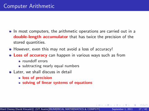
Computer Arithmetic
In most computers, the arithmetic operations are carried out in adouble-length accumulator that has twice the precision of thestored quantities.
However, even this may not avoid a loss of accuracy!
Loss of accuracy can happen in various ways such as from
roundoff errorssubtracting nearly equal numbers
Later, we shall discuss in detail
loss of precisionsolving of linear systems of equations
Ward Cheney/David Kincaid c© (UT Austin[10pt] Engage Learning: Thomson-Brooks/Cole www.engage.com[10pt] www.ma.utexas.edu/CNA/NMC6)NUMERICAL MATHEMATICS & COMPUTING 6th EditionSeptember 1, 2011 17 / 42

Errors: Absolute and Relative
Suppose that α and β are two numbers, of which one is regarded asan approximation to the other.
The error of β as an approximation to α is α− β; that is, the errorequals the exact value minus the approximate value.
The absolute error of β as an approximation to α is
|α− β|
The relative error of β as an approximation to α is
|α− β|/|α|
Notice that in computing the absolute error, the roles of α and β arethe same, whereas in computing the relative error, it is essential todistinguish one of the two numbers as correct.
For practical reasons, the relative error is usually more meaningfulthan the absolute error.
Ward Cheney/David Kincaid c© (UT Austin[10pt] Engage Learning: Thomson-Brooks/Cole www.engage.com[10pt] www.ma.utexas.edu/CNA/NMC6)NUMERICAL MATHEMATICS & COMPUTING 6th EditionSeptember 1, 2011 18 / 42

Absolute/Relative Errors
Absolute Error = |Exact Value−Approximate Value|
Relative Error =|Exact Value−Approximate Value|
|Exact Value|
Here the Exact Value is the True Value.
The Relative Error is related to the Approximate Value rather than tothe Exact Value because the True Value may not be known.
Ward Cheney/David Kincaid c© (UT Austin[10pt] Engage Learning: Thomson-Brooks/Cole www.engage.com[10pt] www.ma.utexas.edu/CNA/NMC6)NUMERICAL MATHEMATICS & COMPUTING 6th EditionSeptember 1, 2011 19 / 42

Example 3
Example
Letα1 = 1.333, β1 = 1.334
α2 = 0.001, β2 = 0.002
What are the absolute errors and relative errors of βi as an approximationto αi ?
The absolute error of βi as an approximation to αi is the same inboth cases—namely, 10−3.
However, the relative errors are 34 × 10−3 and 1, respectively.
The relative error clearly indicates that β1 is a good approximation toα1, but that β2 is a poor approximation to α2.
Ward Cheney/David Kincaid c© (UT Austin[10pt] Engage Learning: Thomson-Brooks/Cole www.engage.com[10pt] www.ma.utexas.edu/CNA/NMC6)NUMERICAL MATHEMATICS & COMPUTING 6th EditionSeptember 1, 2011 20 / 42

Example 4
Example
Considerx = 0.00347 rounded to x = 0.0035
y = 30.158 rounded to y = 30.16
In each case, what are the number of significant digits, absolute errors,and relative errors. Interpret the results.
Case 1: x = 0.35× 10⁻² has two significant digits, absolute error0.3× 10−4, and relative error 0.865× 10⁻².
Case 2: y = 0.3016× 10² has four significant digits, absolute error0.2× 10−2, and relative error 0.66× 10⁻⁴.
Clearly, the relative error is a better indication of the number ofsignificant digits than the absolute error.
Ward Cheney/David Kincaid c© (UT Austin[10pt] Engage Learning: Thomson-Brooks/Cole www.engage.com[10pt] www.ma.utexas.edu/CNA/NMC6)NUMERICAL MATHEMATICS & COMPUTING 6th EditionSeptember 1, 2011 21 / 42
Accuracy and Precision
Accurate to n decimal places means that you can trust n digits tothe right of the decimal place.
Accurate to n significant digits means that you can trust a total ofn digits as being meaningful beginning with the leftmost nonzerodigit.
Ward Cheney/David Kincaid c© (UT Austin[10pt] Engage Learning: Thomson-Brooks/Cole www.engage.com[10pt] www.ma.utexas.edu/CNA/NMC6)NUMERICAL MATHEMATICS & COMPUTING 6th EditionSeptember 1, 2011 22 / 42

Rounding and Chopping
Rounding reduces the number of significant digits in a number.
The result of rounding is a number similar in magnitude that is ashorter number having fewer nonzero digits.
The round-to-even method is also known as statistician’s roundingor bankers’ rounding .
Over a large set of data, the round-to-even rule tends to reduce thetotal rounding error with (on average) an equal portion of numbersrounding up as well as rounding down.
Ward Cheney/David Kincaid c© (UT Austin[10pt] Engage Learning: Thomson-Brooks/Cole www.engage.com[10pt] www.ma.utexas.edu/CNA/NMC6)NUMERICAL MATHEMATICS & COMPUTING 6th EditionSeptember 1, 2011 23 / 42

Example 5
Example
Give some examples of rounding three-decimal numbers to two digits.
Rounding: 0.217 ≈ 0.22, 0.365 ≈ 0.36, 0.475 ≈ 0.48, 0.592 ≈ 0.59
Chopping: 0.217 ≈ 0.21, 0.365 ≈ 0.36, 0.475 ≈ 0.47, 0.592 ≈ 0.59.
On some computers, the user sometimes has the option to have allarithmetic operations done with either chopping or rounding.
The rounding is usually preferable, of course.
Ward Cheney/David Kincaid c© (UT Austin[10pt] Engage Learning: Thomson-Brooks/Cole www.engage.com[10pt] www.ma.utexas.edu/CNA/NMC6)NUMERICAL MATHEMATICS & COMPUTING 6th EditionSeptember 1, 2011 24 / 42

Nested Multiplication
To evaluate the polynomial
p(x) = a0 + a1x + a2x2 + · · ·+ an−1x
n−1 + anxn
group the terms in a nested multiplication:
p(x) = a0 + x(a1 + x(a2 + · · ·+ x(an−1 + x(an)) · · · ))
A pseudocode is a compact and informal description of an algorithmthat uses the conventions of a programming language, but omits thedetailed syntax.
Ward Cheney/David Kincaid c© (UT Austin[10pt] Engage Learning: Thomson-Brooks/Cole www.engage.com[10pt] www.ma.utexas.edu/CNA/NMC6)NUMERICAL MATHEMATICS & COMPUTING 6th EditionSeptember 1, 2011 25 / 42

Pseudocode
Our pseudocode evaluates p(x) starting with the innermostparentheses and working outward.
integer i , n; real p, x ; real array (ai )0:np ← anfor i = n − 1 to 0 do
p ← ai + xpend for
Ward Cheney/David Kincaid c© (UT Austin[10pt] Engage Learning: Thomson-Brooks/Cole www.engage.com[10pt] www.ma.utexas.edu/CNA/NMC6)NUMERICAL MATHEMATICS & COMPUTING 6th EditionSeptember 1, 2011 26 / 42

Horner’s Algorithm/Synthetic Division
This nested multiplication procedure is also known as Horner’salgorithm or synthetic division.
In the pseudocode above, there is exactly one addition and onemultiplication each time the loop is traversed.
Consequently, Horner’s algorithm can evaluate a polynomial with onlyn additions and n multiplications.
This is the minimum number of operations possible.
A naive method of evaluating a polynomial would require many moreoperations.
Ward Cheney/David Kincaid c© (UT Austin[10pt] Engage Learning: Thomson-Brooks/Cole www.engage.com[10pt] www.ma.utexas.edu/CNA/NMC6)NUMERICAL MATHEMATICS & COMPUTING 6th EditionSeptember 1, 2011 27 / 42

Example 6
Example
Show howp(x) = 5 + 3x − 7x2 + 2x3
should be computed.
Letp(x) = 5 + x(3 + x(−7 + x(2)))
for a given value of x .
We have avoided all the exponentiation operations by using nestedmultiplication!
Ward Cheney/David Kincaid c© (UT Austin[10pt] Engage Learning: Thomson-Brooks/Cole www.engage.com[10pt] www.ma.utexas.edu/CNA/NMC6)NUMERICAL MATHEMATICS & COMPUTING 6th EditionSeptember 1, 2011 28 / 42

Polynomial
A polynomial can be written in an alternative form
p(x) =n∑
i=0
aixi =
n∑i=0
(ai
i∏j=1
x
)Utilizing the mathematical symbols for sum
∑and product
∏If n ≤ m, we write
m∑k=n
xk = xn + xn+1 + · · ·+ xm
m∏k=n
xk = xnxn+1 · · · xm
By convention, whenever m < n, we definem∑
k=n
xk = 0,m∏
k=n
xk = 1
Ward Cheney/David Kincaid c© (UT Austin[10pt] Engage Learning: Thomson-Brooks/Cole www.engage.com[10pt] www.ma.utexas.edu/CNA/NMC6)NUMERICAL MATHEMATICS & COMPUTING 6th EditionSeptember 1, 2011 29 / 42

Polynomial (cont.)
Horner’s algorithm can be used in the deflation of a polynomial.
This is the process of removing a linear factor from a polynomial.
If r is a root of the polynomial p, then x − r is a factor of p.
The remaining roots of p are the n − 1 roots of a polynomial q ofdegree 1 less than the degree of p such that
p(x) = (x − r)q(x) + p(r)
whereq(x) = b0 + b1x + b2x
2 + · · ·+ bn−1xn−1
Ward Cheney/David Kincaid c© (UT Austin[10pt] Engage Learning: Thomson-Brooks/Cole www.engage.com[10pt] www.ma.utexas.edu/CNA/NMC6)NUMERICAL MATHEMATICS & COMPUTING 6th EditionSeptember 1, 2011 30 / 42

Pseudocode: Horner’s Algorithm
integer i , n; real p, r ; real array (ai )0:n, (bi )0:n−1bn−1 ← anfor i = n − 1 to 0 do
bi−1 ← ai + rbiend for
Notice thatb−1 = p(r)
If f is an exact root, then
b−1 = p(r) = 0
Ward Cheney/David Kincaid c© (UT Austin[10pt] Engage Learning: Thomson-Brooks/Cole www.engage.com[10pt] www.ma.utexas.edu/CNA/NMC6)NUMERICAL MATHEMATICS & COMPUTING 6th EditionSeptember 1, 2011 31 / 42

Horner’s Algorithm
With pencil and paper, it is often useful to arrange the calculation inHorner’s algorithm like this:
an an−1 an−2 . . . a1 a0r ) rbn−1 rbn−2 . . . rb1 rb0
bn−1 bn−2 bn−3 . . . b0 b−1
Ward Cheney/David Kincaid c© (UT Austin[10pt] Engage Learning: Thomson-Brooks/Cole www.engage.com[10pt] www.ma.utexas.edu/CNA/NMC6)NUMERICAL MATHEMATICS & COMPUTING 6th EditionSeptember 1, 2011 32 / 42
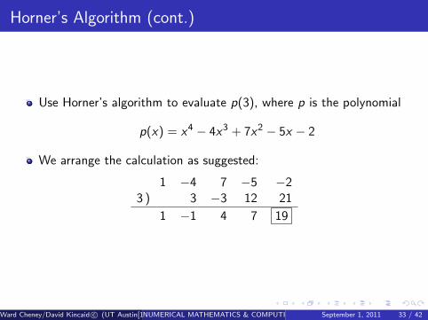
Horner’s Algorithm (cont.)
Use Horner’s algorithm to evaluate p(3), where p is the polynomial
p(x) = x4 − 4x3 + 7x2 − 5x − 2
We arrange the calculation as suggested:
1 −4 7 −5 −23 ) 3 −3 12 21
1 −1 4 7 19
Ward Cheney/David Kincaid c© (UT Austin[10pt] Engage Learning: Thomson-Brooks/Cole www.engage.com[10pt] www.ma.utexas.edu/CNA/NMC6)NUMERICAL MATHEMATICS & COMPUTING 6th EditionSeptember 1, 2011 33 / 42

Example 7 (cont.)
Thus, we obtain p(3) = 19, and
p(x) = (x − 3)(x3 − x2 + 4x + 7) + 19
In the deflation process, if r is a zero of the polynomial p, thenx − r is a factor of p, and conversely.
The remaining zeros of p are the n − 1 zeros of q(x).
Ward Cheney/David Kincaid c© (UT Austin[10pt] Engage Learning: Thomson-Brooks/Cole www.engage.com[10pt] www.ma.utexas.edu/CNA/NMC6)NUMERICAL MATHEMATICS & COMPUTING 6th EditionSeptember 1, 2011 34 / 42

Example 8
Example
Deflate the polynomial
p(x) = x4 − 4x3 + 7x2 − 5x − 2
using the fact that 2 is one of its zeros.
We use the same arrangement of computations as before:
1 −4 7 −5 −22 ) 2 −4 6 2
1 −2 3 1 0
Thus, we have p(2) = 0, and
x4 − 4x3 + 7x2 − 5x − 2 = (x − 2)(x3 − 2x2 + 3x + 1)
Ward Cheney/David Kincaid c© (UT Austin[10pt] Engage Learning: Thomson-Brooks/Cole www.engage.com[10pt] www.ma.utexas.edu/CNA/NMC6)NUMERICAL MATHEMATICS & COMPUTING 6th EditionSeptember 1, 2011 35 / 42
Pairs of Easy/Hard Problems
Sometimes in scientific computing, we encounter a pair of problems,one of which is easy and the other hard and they are inverses of eachother.
In cryptology, multiplying two numbers together is trivial, but thereverse problem (factoring a huge number) verges on the impossible!
Given the roots, the power form of the polynomial is easily, but giventhe polynomial it may be a hard problem to compute the roots.
Given A and b, computing b = Ax is trivial, but finding x from A andb (matrux inverse) may be hard.
In two-point boundary value problems, finding Df , f (0), and f (1)when f is given and D is a differential operator is easy, but finding ffrom knowledge of Df , f (0) and f (1) may be hard.
In general, computing the eigenvalues and eigenvectors of a matrixA may be a hard problem, but given the eigenvalues and eigenvectorsit is easy to determine the matrix A.
Ward Cheney/David Kincaid c© (UT Austin[10pt] Engage Learning: Thomson-Brooks/Cole www.engage.com[10pt] www.ma.utexas.edu/CNA/NMC6)NUMERICAL MATHEMATICS & COMPUTING 6th EditionSeptember 1, 2011 36 / 42

First Programming Experiment
Consider, from the computational point of view, taking thederivative of a function.
The derivative of a function f at a point x is defined by the equation
f ′(x) = limh→0
f (x + h)− f (x)
h
A computer has the capacity of imitating the limit operation by usinga sequence of numbers h such as
h = 4−1, 4−2, 4−3, . . . , 4−n, . . . (approaching zero rapidly)
The sequence 1/4n consists of machine numbers in a binary computerand, on a 32-bit computer, it is sufficiently close to zero when n = 10.
If f (x) = sin x , here is pseudocode for computing f ′(x) at the pointx = 0.5
Ward Cheney/David Kincaid c© (UT Austin[10pt] Engage Learning: Thomson-Brooks/Cole www.engage.com[10pt] www.ma.utexas.edu/CNA/NMC6)NUMERICAL MATHEMATICS & COMPUTING 6th EditionSeptember 1, 2011 37 / 42

Pseudocode First
program Firstinteger i , imax, n← 30real error, y , x ← 0.5, h← 1, emin← 1for i = 1 to n
h← 0.25hy ← [sin(x + h)− sin(x)]/herror← |cos(x)− y |;output i , h, y , errorif error < emin thenemin← error; imin← i
end ifend foroutput imin, eminend program First
Ward Cheney/David Kincaid c© (UT Austin[10pt] Engage Learning: Thomson-Brooks/Cole www.engage.com[10pt] www.ma.utexas.edu/CNA/NMC6)NUMERICAL MATHEMATICS & COMPUTING 6th EditionSeptember 1, 2011 38 / 42

So what?
We have neither explained the purpose of the experiment nor shownthe output from this pseudocode.
We invite the student to discover this by coding and running it on acomputer.
Explain the results.
Ward Cheney/David Kincaid c© (UT Austin[10pt] Engage Learning: Thomson-Brooks/Cole www.engage.com[10pt] www.ma.utexas.edu/CNA/NMC6)NUMERICAL MATHEMATICS & COMPUTING 6th EditionSeptember 1, 2011 39 / 42
Mathematical Software
The algorithms and programming problems have been coded andtested in a variety of ways.
They are available on the website:
www.ma.utexas.edu/CNA/NMC6
It is instructive to utilize mathematical software systems such as
MATLABMapleMathematica
since they contain built-in problem-solving procedures.
Ward Cheney/David Kincaid c© (UT Austin[10pt] Engage Learning: Thomson-Brooks/Cole www.engage.com[10pt] www.ma.utexas.edu/CNA/NMC6)NUMERICAL MATHEMATICS & COMPUTING 6th EditionSeptember 1, 2011 40 / 42

Summary 1.1
Use nested multiplication to evaluate a polynomial efficiently:
p(x) = a0 + a1x + a2x2 + · · ·+ an−1x
n−1 + anxn
= a0 + x(a1 + x(a2 + · · ·+ x(an−1 + x(an)) · · · ))
Pseudocode is
p ← anfor k = 1 to n
p ← xp + an−kend for
Ward Cheney/David Kincaid c© (UT Austin[10pt] Engage Learning: Thomson-Brooks/Cole www.engage.com[10pt] www.ma.utexas.edu/CNA/NMC6)NUMERICAL MATHEMATICS & COMPUTING 6th EditionSeptember 1, 2011 41 / 42
Summary 1.1 (cont.)
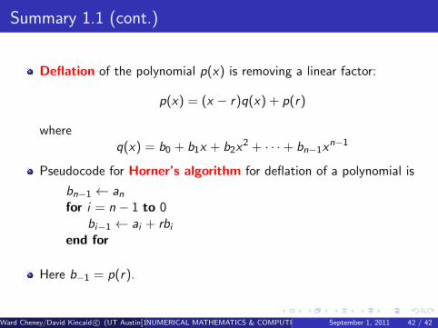
Deflation of the polynomial p(x) is removing a linear factor:
p(x) = (x − r)q(x) + p(r)
whereq(x) = b0 + b1x + b2x
2 + · · ·+ bn−1xn−1
Pseudocode for Horner’s algorithm for deflation of a polynomial is
bn−1 ← anfor i = n − 1 to 0
bi−1 ← ai + rbiend for
Here b−1 = p(r).
Ward Cheney/David Kincaid c© (UT Austin[10pt] Engage Learning: Thomson-Brooks/Cole www.engage.com[10pt] www.ma.utexas.edu/CNA/NMC6)NUMERICAL MATHEMATICS & COMPUTING 6th EditionSeptember 1, 2011 42 / 42