numerical investigation of flow past a circular cylinder and in a
TRANSCRIPT
LAPPEENRANTA UNIVERSITY OF TECHNOLOGYFaculty of TechnologyDepartment of Mathematics and Physics
Numerical Investigation of Flow Past aCircular Cylinder and in a Staggered TubeBundle Using Various Turbulence Models
The topic of this Master’s thesis was approved by the departmental council of the De-partment of Mathematics and Physics on 27th May, 2010.
Supervisors: Professor Heikki HaarioAssociate Professor Teemu Turunen-Saaresti
Examiners: Professor Heikki HaarioAssociate Professor Teemu Turunen-Saaresti
In Lappeenranta August 24, 2010
Yogini PatelTeknologiapuistonkatu 2 B 2853850 LappeenrantaPhone: +358466175120Email: [email protected] & [email protected]

Abstract
Lappeenranta University of TechnologyDepartment of Mathematics and Physics
Yogini Patel
Numerical Investigation of Flow Past a Circular Cylinder and in a StaggeredTube Bundle Using Various Turbulence ModelsMaster’s thesis
2010
87 pages, 48 figures, 13 tables
Key words: Turbulent flow, RANS models, Large eddy simulation, Circular cylinder,Vortex shedding, Tube bundle.
Transitional flow past a three-dimensional circular cylinder is a widely studied phe-nomenon since this problem is of interest with respect to many technical applications.In the present work, the numerical simulation of flow past a circular cylinder, performedby using a commercial CFD code (ANSYS Fluent 12.1) with large eddy simulation (LES)and RANS (κ−ε and Shear-Stress Transport (SST) κ−ω model) approaches. The turbu-lent flow for ReD = 1000 & 3900 is simulated to investigate the force coefficient, Strouhalnumber, flow separation angle, pressure distribution on cylinder and the complex threedimensional vortex shedding of the cylinder wake region. The numerical results extractedfrom these simulations have good agreement with the experimental data (Zdravkovich,1997). Moreover, grid refinement and time-step influence have been examined.
Numerical calculations of turbulent cross-flow in a staggered tube bundle continues toattract interest due to its importance in the engineering application as well as the factthat this complex flow represents a challenging problem for CFD. In the present worka time dependent simulation using κ − ε, κ − ω and SST models are performed in twodimensional for a subcritical flow through a staggered tube bundle. The predicted turbu-lence statistics (mean and r.m.s velocities) have good agreement with the experimentaldata (S. Balabani, 1996). Turbulent quantities such as turbulent kinetic energy anddissipation rate are predicted using RANS models and compared with each other. Thesensitivity of grid and time-step size have been analyzed. Model constants sensitivitystudy have been carried out by adopting κ− ε model. It has been observed that modelconstants are very sensitive to turbulence statistics and turbulent quantities.
i

AcknowledgementsIn the first place I would like to record my gratitude to the Department of Mathematicsfrom Lappeenranta University of Technology for financing of my studies.
I would like to express my deepest sense of gratitude to my supervisor, Professor HeikkiHaario, for his patient guidance, encouragement, understanding and excellent advicethroughout this thesis as well as providing me all facilities during my thesis.
My sincere appreciation goes to Associate Professor Teemu Turunen-Saaresti for hisconstant support, great advice and comments, directing and assistance during the workof this thesis, which appointed him a backbone of this work. I attribute the level of mythesis to his encouragement and effort and without him this thesis, too, would not havebeen completed or written.
Most important thanks here goes to my best friend, Gitesh. I don’t know what mylife would be without you. You are like the sunshine, always giving me the feeling ofwarmth, hope and peace. It is so wonderful to have you beside me, in the past, present,and future. So Thank you so much for your faithful love and endless help. I could say,without you, this thesis wouldn’t exist.
I am also grateful to all my friends in Lappeenranta who helped me to have enjoyableand memorial stay.
Where would I be without my family? None of this would have been possible without thelove and patience of my family. My parents deserve special mention for their inseparablesupport and prayers. My dad, Natvarlal, in the first place is the person who put thefundament my learning character, showing me the joy of intellectual pursuit ever since Iwas a child. My mom, Kantaben, is the one who sincerely raised me with her caring andunconditional love. I convey special acknowledgement to my elder brother, Alpeshbhai,and his wife, Deepali, for their support and love. I would like to express the dearestthanks to my niece, Aastha, for her loving support. I am extending my sincere gratitudeto my kind grandparents for their blessings. I dedicate this thesis to my family andGitesh, the most special person in my life.
I am ever grateful to Lord Shiva, the Creator and the Guardian, and to whom I owe myvery existence.
Lappeenranta, August 24, 2010
Yogini Patel
ii

Contents
1 Introduction 1
1.1 Objectives of the thesis . . . . . . . . . . . . . . . . . . . . . . . . . . . . . 1
1.2 Thesis structure . . . . . . . . . . . . . . . . . . . . . . . . . . . . . . . . . 2
2 Theoretical background 4
2.1 Governing equations of fluid flow . . . . . . . . . . . . . . . . . . . . . . . 4
2.1.1 Continuity equation . . . . . . . . . . . . . . . . . . . . . . . . . . 4
2.1.2 Momentum equation . . . . . . . . . . . . . . . . . . . . . . . . . . 5
2.1.3 Navier-Stokes equations for a Newtonian fluid . . . . . . . . . . . . 7
2.2 Overview of Computational Fluid Dynamics(CFD) . . . . . . . . . . . . . 9
2.3 What is turbulence ? . . . . . . . . . . . . . . . . . . . . . . . . . . . . . . 11
2.4 History of turbulence . . . . . . . . . . . . . . . . . . . . . . . . . . . . . . 11
3 Turbulence models 14
3.1 Classification of turbulence models . . . . . . . . . . . . . . . . . . . . . . 14
3.2 Large eddy simulation (LES) . . . . . . . . . . . . . . . . . . . . . . . . . 18
3.2.1 Filtering of Navier-Stokes equations . . . . . . . . . . . . . . . . . 18
3.2.2 Smagorinksy-Lilly SGS model . . . . . . . . . . . . . . . . . . . . . 21
3.3 Reynolds-averaged Navier-Stokes equations . . . . . . . . . . . . . . . . . 23
3.3.1 Standard κ− ε model . . . . . . . . . . . . . . . . . . . . . . . . . 26
3.3.2 Standard κ− ω model . . . . . . . . . . . . . . . . . . . . . . . . . 27
3.3.3 Shear-Stress Transport (SST) κ− ω model . . . . . . . . . . . . . . 28
3.4 The law of the wall . . . . . . . . . . . . . . . . . . . . . . . . . . . . . . . 30
4 Flow past a circular cylinder 33
4.1 Conceptual overview of flow past a circular cylinder . . . . . . . . . . . . . 33
iii

4.1.1 Reynolds number . . . . . . . . . . . . . . . . . . . . . . . . . . . . 33
4.1.2 Vortex shedding and Strouhal number . . . . . . . . . . . . . . . . 34
4.1.3 Drag, lift and pressure coefficients . . . . . . . . . . . . . . . . . . 35
4.2 Computational details . . . . . . . . . . . . . . . . . . . . . . . . . . . . . 36
4.3 Results and Discussions . . . . . . . . . . . . . . . . . . . . . . . . . . . . 40
4.3.1 Discussion of the test case with ReD = 1000 . . . . . . . . . . . . . 40
4.3.2 Discussion of the test case with ReD = 3900 . . . . . . . . . . . . . 45
4.3.3 Grid sensitivity study with ReD = 1000 . . . . . . . . . . . . . . . 50
4.3.4 Effect of time-step size with LES . . . . . . . . . . . . . . . . . . . 55
5 Flow past in a staggered tube bundle 58
5.1 Computational details . . . . . . . . . . . . . . . . . . . . . . . . . . . . . 59
5.2 Results and Discussions . . . . . . . . . . . . . . . . . . . . . . . . . . . . 62
5.2.1 Comparison between simulated and experimental results . . . . . . 63
5.2.2 Grid independence tests . . . . . . . . . . . . . . . . . . . . . . . . 68
5.2.3 Time-step sensitivity study . . . . . . . . . . . . . . . . . . . . . . 73
5.2.4 Sensitivity of the model constants C1ε and C2ε in κ− ε model . . 76
6 Conclusions 83
References 86
iv

List of Tables
1 Simulation settings for flow past a circular cylinder case with RANS models 39
2 Simulation settings for flow past a circular cylinder case with LES model . 39
3 Experimental and computational results for ReD = 1000 . . . . . . . . . 41
4 Experimental and computational results for ReD = 3900 . . . . . . . . . 45
5 Details of grids used in mesh-independence tests . . . . . . . . . . . . . . 50
6 Drag coefficient of the flow past a circular cylinder using the RANS models 51
7 Computed flow parameters in comparison with experimental results usingLES . . . . . . . . . . . . . . . . . . . . . . . . . . . . . . . . . . . . . . . 51
8 CPU times details used by each model for different grids. . . . . . . . . . 55
9 Effect of time-step size on the Cd and St using LES. . . . . . . . . . . . . 56
10 Simulation settings of flow past in a staggered tube bundle case . . . . . . 62
11 Details of grids used in mesh-independence tests and their y+ values . . . 68
12 Averaged difference in the prediction of turbulent kinetic energy and dis-sipation rate with respect to original C1ε . . . . . . . . . . . . . . . . . . . 79
13 Averaged difference in the prediction of turbulent kinetic energy and dis-sipation rate with respect to original C2ε . . . . . . . . . . . . . . . . . . . 82
v

List of Figures
1 (a) Fluid element for conservation laws (b) mass flows in and out of fluidelement . . . . . . . . . . . . . . . . . . . . . . . . . . . . . . . . . . . . . 4
2 (a) Stress components on three faces of fluid element (b) stress componentsin the x-direction . . . . . . . . . . . . . . . . . . . . . . . . . . . . . . . . 6
3 Overview of the CFD . . . . . . . . . . . . . . . . . . . . . . . . . . . . . . 10
4 Turbulence models classification . . . . . . . . . . . . . . . . . . . . . . . . 14
5 Extend of modelling for certain types of turbulent models [21] . . . . . . . 18
6 Subdivisions of the Near-Wall Region [8] . . . . . . . . . . . . . . . . . . . 31
7 Vortex shedding in the wake region of the flow past a circular cylinder [31]. 34
8 Diagram of forces acting around a circular cylinder. . . . . . . . . . . . . . 35
9 Computational geometry and boundary conditions. . . . . . . . . . . . . . 37
10 (a) Computational domain, (b) grid around the cylinder, and (c) 3D closerview of the cylinder. . . . . . . . . . . . . . . . . . . . . . . . . . . . . . . 38
11 Time histories of (a) drag coefficient,Cd, and (b) lift coefficient, Cl, for LES. 41
12 Pressure coefficient distribution around circular cylinder at ReD = 1000. . 42
13 Iso-surfaces of x-vorticity produced from ske and SST models with ReD =1000. . . . . . . . . . . . . . . . . . . . . . . . . . . . . . . . . . . . . . . . 43
14 Iso-surfaces of instantaneous x-vorticity with ReD = 1000. . . . . . . . . . 43
15 Contours of velocity magnitude and velocity vector with ReD = 1000. . . 44
16 Cl history for κ− ε and SST with ReD = 3900. . . . . . . . . . . . . . . . 45
17 Cd and Cl histories for LES with ReD = 3900. . . . . . . . . . . . . . . . . 46
18 Drag coefficient of the flow past a circular cylinder compared to experi-mental data. . . . . . . . . . . . . . . . . . . . . . . . . . . . . . . . . . . . 47
19 Pressure coefficient distribution around circular cylinder at ReD = 3900. . 47
20 Iso-surfaces of x-vorticity produced from ske and SST models with ReD =3900. . . . . . . . . . . . . . . . . . . . . . . . . . . . . . . . . . . . . . . . 48
vi

21 Iso-surfaces of instantaneous x-vorticity with ReD = 3900. . . . . . . . . . 49
22 Cd and Cl histories with different grids for LES. . . . . . . . . . . . . . . . 52
23 Iso-surface of the magnitude of instantaneous vorticity for LES with (a)Grid A, (b) Grid B, and (c) Grid C. . . . . . . . . . . . . . . . . . . . . . 53
24 Contour of x-velocity for LES with (a) Grid A, (b) Grid B, and (c) Grid C. 54
25 Cd and Cl histories with different timestep size. . . . . . . . . . . . . . . . 56
26 Strouhal number of the flow past a circular cylinder compared to experi-mental data. . . . . . . . . . . . . . . . . . . . . . . . . . . . . . . . . . . . 57
27 Iso-surface of instantaneous x-vorticity for LES using different time-step. . 57
28 (a) Cross-sectional view of the tube bundle, and (b) locations at whichresults are presented. . . . . . . . . . . . . . . . . . . . . . . . . . . . . . . 60
29 (a) Boundary conditions, (b) computational grid, and (C) closer view ofthe tube surface. . . . . . . . . . . . . . . . . . . . . . . . . . . . . . . . . 61
30 Contours of U-component of velocity (a-c) and vorticity magnitude (d-f). . 63
31 Contours of velocity vectors of SST model. . . . . . . . . . . . . . . . . . . 64
32 Comparison between profiles of predicted streamwise mean velocity withexperimental values at selected axial locations. . . . . . . . . . . . . . . . 65
33 Comparison between profiles of predicted transverse mean velocity withexperimental values at selected axial locations. . . . . . . . . . . . . . . . 66
34 Comparison between profiles of predicted streamwise fluctuations of thevelocity component with experimental values at selected axial locations. . 67
35 Comparison the predicted dissipation rate at selected x/d locations. . . . . 68
36 Contours of turbulent kinetic energy with (a) Grid A, (b) Grid B, (c) GridC, and (d) Grid D using SST model. . . . . . . . . . . . . . . . . . . . . . 69
37 Contours of U-component of velocity with (a) Grid A, (b) Grid B, (c)Grid C, and (d) Grid D using SST model. . . . . . . . . . . . . . . . . . . 69
38 Profiles of grid-independence test of streamwise mean velocity at x/d =1.25 and 5.45. . . . . . . . . . . . . . . . . . . . . . . . . . . . . . . . . . . 71
vii

39 Profiles of grid-independence test of transverse mean velocity at x/d =1.25 and 5.45. . . . . . . . . . . . . . . . . . . . . . . . . . . . . . . . . . . 72
40 Profiles of grid-independence test of turbulent kinetic energy at x/d = 1.25and 5.45. . . . . . . . . . . . . . . . . . . . . . . . . . . . . . . . . . . . . 73
41 Time-step effect on streamwise mean velocity at x/d = 3.35 and 5.45. . . . 74
42 Time-step effect on transverse mean velocity at x/d = 3.35 and 5.45. . . . 75
43 Comparison between profiles of predicted streamwise (a-d) and transverse(e-f) mean velocities with experimental values at selected axial locations. . 77
44 Comparison the predicted turbulent kinetic energy at selected x/d locations. 78
45 Comparison the predicted dissipation rate at selected x/d locations. . . . . 78
46 Comparison between profiles of predicted streamwise (a-d) and transverse(e-f) mean velocity with experimental values at selected axial locations. . 80
47 Comparison the predicted turbulent kinetic energy at selected x/d locations. 81
48 Comparison the predicted dissipation rate at selected x/d locations. . . . . 81
viii

Nomenclature
A projected area [m2]
B additive constant
C1ε, C2ε model constants
Cd drag coefficient
Cl lift coefficient
Cp pressure coefficient
CSGS sub-grid scale constant
d tube diameter [m]
D diameter of the cylinder [m]
f force [N ]
fs Strouhal frequency [Hz]
k von karamn’s constant
N number of nodes
p pressure [Nm−2]
Re Reynolds number
S source term
SL longitudinal pitch-to-diameter ratio
St Strouhal number
ST transverse pitch-to-diameter ratio
t time [s]
u velocity [ms−1]
u′ fluctuation velocity [ms−1]
ix

U x-direction mean velocity component [ms−1]
U∞ approach velocity [ms−1]
V y-direction mean velocity component [ms−1]
x streamwise coordinate [m]
y transverse coordinate [m]
y+ non-dimensional normal distance from wall
Greek Letters
∆ filter cutoff width [m]
ε turbulent dissipation rate [m2s−3]
εk dissipation term in the turbulent kinetic energy budget [m2s−3]
θ separation angle [degree]
` turbulent length scale [m]
κ turbulent kinetic energy [m2s−2]
λ viscosity [m2s−1]
µ dynamic viscosity [Nsm−2]
µt turbulent viscosity [Nsm−2]
ρ density [kgm−3]
σ Prandtl number
τ viscous stress [Nm−2]
ϑ velocity scale [ms−1]
φ filtered function
ω specific dissipation [s−1]
x

Abbreviations
CFD Computational Fluid Dynamics
DES Detached Eddy Simulation
DNS Direct Numerical Simulation
DSM Dynamic Smagorinsky Model
EVM Eddy-viscosity Models
FFT Fast Fourier Transform
FVM Finite Volume Method
LDA Laser Doppler Anemometry
LES Large Eddy Simulation
PDE Partial Differential Equation
RANS Reynolds-averaged Navier-Stokes
RSM Reynolds Stress Model
SGS Sub-grid Scale Stresses
ske standard κ− ε
SST Shear-Stress Transport
TKE Turbulent Kinetic Energy
Subscript or Superscript
d, l referring drag and lift respectively
i, j referring i- and j-directions respectively
x, y, z referring to x-, y- and z-directions respectively
xi

1 Introduction
The topic of this thesis is the numerical investigation of flow past a circular cylinderand in a staggered tube bundle using various turbulence models. Computational FluidDynamics (CFD) calculates numerical solutions using the equations governing fluid flow.One of the classical problems in fluid mechanics is the determination of the flow fieldpast a bluff body represented by a circular or rectangular cylinder. The flow past circularcylinders has been extensively studied due to its importance in many practical applica-tions, such as heat exchangers, chimneys, hydrodynamic loading on ocean marine pilesand offshore platform risers and support legs [12]. In scientific terms, the flow aroundcircular cylinders includes a variety of fluid dynamics phenomena, such as separation,vortex shedding and the transition to turbulence. The mechanisms of vortex sheddingand its suppression have significant effects on the various fluid-mechanical properties ofpractical interest: flow-induced forces such as drag and lift forces and pressure coefficient.
Furthermore, the predictions of turbulent cross-flow in a staggered tube bundle contin-ues to attract interest due to its importance in the engineering application as well as thefact that this complex flow represents a challenging problem for CFD. Cross-flow in tubebundles has wide practical applications in the design of heat exchangers, in flow acrossoverhead cables, and in cooling systems for nuclear power plants [13]. In addition to thecomplexity arising from the flow instabilities in the tube bundle, one must also considerwhether the flow is turbulent or laminar. Flows in tube bundles are usually subcritical(mixed, transition to turbulence occurs after separation) or critical (predominantly tur-bulent, only part of the boundary layer developing on the tube surface is laminar). Incritical flows, transition to turbulence occurs before separation and turbulence is promi-nent in the rest of the boundary layer and in the flow inside the bundle (Zukauskas, 1989).The combination of the flow instabilities and the transitional phenomena present in theboundary layers makes this type of flow difficult to model numerically. To appropriatelysimulate these flow characteristics, various turbulence models in CFD are used.
1.1 Objectives of the thesis
The objectives of the thesis have been set as follows:
• To investigate the flow past a circular cylinder, which is sensitive to changes ofReynolds number. Two Reynolds numbers (1000 and 3900) have been tested usingunsteady turbulence models such as the RANS turbulence models namely, theκ − ε model and the Shear-Stress Transport (SST) κ − ω model, and the LargeEddy Simulation (LES). The study includes the simulation of vortex sheddingphenomenon, force coefficient, Strouhal number and pressure distribution of the
1

flow. The numerical results extracted from CFD simulations are compared witheach other (κ − ε model, SST model and LES model) and with the experimentaldata in order to determine the relative performance of these turbulence models andto find the best model for the flow of interest. Furthermore, grid-independence testsand time integration are performed to investigate the influence of grid refinementand time-step size effect respectively on the solution.
• In a staggered tube bundle case, time dependent calculations of the subcriticalcross flow through a tube bundle have been performed in two dimensions withRANS models. RANS turbulence models like, the κ − ε model, the κ − ω modeland the SST model have been chosen to test the suitability and the applicability ofthe models on the flow past a staggered tube bundle. For models comparison pur-pose, the streamwise and transverse, mean and r.m.s velocities are compared withexperimental data at different location. Turbulent quantities such as turbulent ki-netic energy and dissipation rate are calculated using RANS models and comparedwith each other. Moreover, grid and time-step size sensitivity are performed usingabove mentioned turbulence models.
1.2 Thesis structure
This chapter consists of the objectives and the methodology of the thesis work. Thereader is then introduced to the main content of the following chapters.
Chapter 2, discusses the theoretical background of basic equations describing fluid mo-tion. It explains how CFD formulates those equations. By using those equations, theNavier-Stokes equations are derived. In the middle part of this chapter discusses theprinciples of the CFD. The last part describes the definition of turbulence and its richhistory.
Chapter 3 gives the brief details of turbulence models. The classification of the modelsare discussed based on filtering and time averaging. Different turbulence models suchas the large eddy simulation (LES) and the Reynolds Averaged Navier-Stokes (RANS)models are explained with the suitability of each model in the applications of the flowpast a circular cylinder and in a staggered tube bundle. The end part of this chaptercontains the information about law of the wall.
Chapter 4 presents work done on the flow past a circular cylinder using RANS andLES methods at two different Reynolds numbers. The chapter focuses mainly on theverification and validation of RANS models and LES on the flow past a circular cylinder.Pressure distribution, as well as the comparison of the Strouhal number and the dragcoefficient of the flow from the prediction of RANS models and LES are compared to
2
experimental data. Grid and time-step size effect cases are discussed at the end also.
Chapter 5 contains work done on the flow past in a staggered tube bundle. The be-ginning part of this chapter displays the information about the staggered tube bundle.The chapter focuses on the applicability and suitability of RANS models with presentapplication and compared with experimental results. At the end, results obtained fromCFD simulations for grid and time-step size influences are studied.
Chapter 6 draws conclusions of the whole thesis. This focuses on the objectives of thework and how they are achieved throughout the thesis.
3

2 Theoretical background
This chapter is a review of general theory of the governing equations for fluid flow. Thegoverning equations of fluid flow are called the Navier-Stokes equations. In this section,concisely we will discuss the principles of the CFD with its components. Moreover,fundamental description of turbulence and its history will demonstrate.
2.1 Governing equations of fluid flow
In mid 18th century, the French engineer Claude Navier and the Irish mathematicianGeorge Stokes derived the well-known equations of fluid motion, known as the Navier-Stokes equations. These equations have been derived based on the fundamental govern-ing equations of fluid dynamics, called the continuity, the momentum and the energyequations, which represent the conservation laws of physics [15].
2.1.1 Continuity equation
Figure 1: (a) Fluid element for conservation laws (b) mass flows in and out of fluidelement
In Figure 1a, the six faces are labeled N, S, E, W, T and B, which stands for North,South, East, West, Top and Bottom. The centre of the element is located at position (x,y, z). The derivation of the mass conservation equation is to write down a mass balancefor the element:Rate of increase of mass in fluid element = Net rate of flow of mass into fluid element[1]The rate of increase of mass in the fluid element is
4

∂(ρδxδyδz)∂t
=∂ρ
∂tδxδyδz (1)
Next we need to account flow rate across a face of the element, which is given by theproduct of density, area and the velocity component normal to the face. From Figure 1bit can be seen that the net rate of flow of mass into the element across its boundaries isgiven by
(ρu− ∂(ρu)
∂x
12δx
)δyδz −
(ρu+
∂(ρu)∂x
12δx
)δyδz
+(ρv − ∂(ρv)
∂y
12δy
)δxδz −
(ρv +
∂(ρv)∂y
12δy
)δxδz
+(ρw − ∂(ρw)
∂z
12δz
)δxδy −
(ρw +
∂(ρw)∂w
12δz
)δxδz (2)
The rate of increase of mass inside the element from equation (1) is now equated tothe net rate of flow of into the element across its faces from equation (2). All terms ofthe resulting mass balance are arranged on the left hand side of the equals sign and theexpression is divided by the element volume δxδyδz [2]. This yields
∂ρ
∂t+∂(ρu)∂x
+∂(ρv)∂y
+∂(ρw)∂z
= 0 (3)
Or in vector notation
∂ρ
∂t+ div(ρu) = 0 (4)
Equation (4) is the unsteady, three-dimensional mass conservation or continuity equationat a point in a compressible fluid [1].
For an incompressible fluid the density ρ is constant and equation (4) becomes
div u = 0 (5)
2.1.2 Momentum equation
Newton’s second law states that [1]:Rate of increase of momentum of fluid particle = Sum of forces on fluid particle
5

The rates of increase of x-, y- and z-momentum per unit volume of a fluid particle aregiven by
ρDu
DtρDv
DtρDw
Dt(6)
Now, the state of stress of a fluid element is defined in terms of the pressure and thenine viscous stress components which is shown in Figure 2a.
Figure 2: (a) Stress components on three faces of fluid element (b) stress components inthe x-direction
The pressure, a normal stress, is denoted by p. Viscous stresses are denoted by τ . Thesuffix notation τij is applied to indicate the direction of the viscous stresses. The suffices iand j in τij indicate that the stress component acts in the j - direction on a surface normalto the i-direction. First we consider the x -components of the forces due to pressure pand stress components τxx, τyx and τzx which is shown in Figure 2b. Forces aligned withthe direction of a co-ordinate axis get a positive sign and those in the opposite directiona negative sign. The net force in the x -direction is the sum of the force componentsacting in that direction on the fluid element.
On the pair of faces (E, W) we have
[(p− ∂p
∂x
12δx
)−(τxx −
∂τxx∂x
12δx
)]δyδz
+[−(p+
∂p
∂x
12δx
)+(τxx +
∂τxx∂x
12δx
)]δyδz =
(−∂p∂x
+∂τxx∂x
)δxδyδz (7)
The net force in the x -direction on the pair of faces (N, S) is
6

−(τyx −
∂τyx∂y
12δy
)δxδz +
(τyx +
∂τyx∂y
12δy
)δxδz =
∂τyx∂y
δxδyδz (8)
And the net force in the x -direction on faces T and B is given by
−(τzx −
∂τzx∂z
12δz
)δxδy +
(τzx +
∂τzx∂z
12δz
)δxδy =
∂τzx∂z
δxδyδz (9)
The total force per unit volume on the fluid due to these surface stresses is equal to thesum of equations (7), (8) and (9) divided by the volume δxδyδz.
∂(−p+ τxx)∂x
+∂τyx∂y
+∂τzx∂z
(10)
In addition, the body forces are not consider in the above explanation. In further detailtheir overall effect can be included by defining a source SMx of x -momentum per unitvolume per unit time. The x -component of the momentum equation is found by settingthe rate of change of x -momentum of the fluid particle in equation(6) equal to the totalforce in the x -direction on the element due to surface stresses in equation(10) plus therate of increase of x -momentum due to sources
ρDu
Dt=∂(−p+ τxx)
∂x+∂τyx∂y
+∂τzx∂z
+ SMx (11)
Similarly we can verify the y-component of the momentum equation is given by
ρDv
Dt=∂τxy∂x
+∂(−p+ τyy)
∂y+∂τzy∂z
+ SMy (12)
And the z -component of the momentum equation by
ρDw
Dt=∂τxz∂x
+∂τyz∂y
+∂(−p+ τzz)
∂z+ SMz (13)
The source terms SMx, SMy and SMz in above equations include contributions due tobody forces only.
2.1.3 Navier-Stokes equations for a Newtonian fluid
The most useful forms of the conservation equation for fluid flows are obtained by in-troducing a suitable model for the viscous stresses τij . In many fluid flows the viscous
7

stresses can be expressed as functions of the local deformation rate or strain rate [1]. Inthree dimensional flows, the local rate of deformation is composed of the linear defor-mation rate and the volumetric deformation rate. The rate of linear deformation of afluid element has nine components in three dimensions, six of which are independent inisotropic fluid. they are denoted by the symbol sij .
In a Newtonian fluid the viscous stresses are proportional to the rates of deformation [2].The three dimensional form of Newton’s law of viscosity for compressible flows involvestwo constants of proportionality: 1) dynamic viscosity, µ, to relate stresses to lineardeformation, and 2) viscosity, λ, to relate stresses to the volumetric deformation. Theviscous stress components, of which six are independent, are
τxx = 2µ∂u
∂x+ λ div u τyy = 2µ
∂v
∂y+ λ div u τzz = 2µ
∂w
∂z+ λ div u
τxy = τyx = µ
(∂u
∂y+∂v
∂x
)τxz = τzx = µ
(∂u
∂z+∂w
∂x
)
τyz = τzy = µ
(∂v
∂z+∂w
∂y
)(14)
The second viscosity λ is not known much because of its effect is small in practice.Substitution of the above shear stresses equation(14) into equations(11), (12) and (13)yields the so-called Navier-Stokes equations.
ρDu
Dt= −∂p
∂x+
∂
∂x
[2µ∂u
∂x+ λ div u
]+
∂
∂y
[µ
(∂u
∂y+∂v
∂x
)]+∂
∂z
[µ
(∂u
∂z+∂w
∂x
)]+ SMx (15)
ρDv
Dt= −∂p
∂y+
∂
∂x
[µ
(∂u
∂y+∂v
∂x
)]+
∂
∂y
[2µ∂v
∂y+ λ div u
]+∂
∂z
[µ
(∂v
∂z+∂w
∂y
)]+ SMy (16)
ρDw
Dt= −∂p
∂z+
∂
∂x
[µ
(∂u
∂z+∂w
∂x
)]+
∂
∂y
[µ
(∂v
∂z+∂w
∂y
)]+∂
∂z
[2µ∂w
∂z+ λ div u
]+ SMz (17)
8

Now, rearrange the viscous stress terms as follows:
∂
∂x
[2µ∂u
∂x+ λ div u
]+
∂
∂y
[µ
(∂u
∂y+∂v
∂x
)]+
∂
∂z
[µ
(∂u
∂z+∂w
∂x
)]= div(µ grad u) + [sMx]
the viscous stresses in the y- and z -component equations can be rearrange in a similarmanner. And defining a new source terms by
SN = SM + [sM ] (18)
Finally the Navier-Stokes equations can be written in the most useful form is
ρDu
Dt= −∂p
∂x+ div(µ grad u) + SNx (19)
ρDv
Dt= −∂p
∂y+ div(µ grad v) + SNy (20)
ρDw
Dt= −∂p
∂z+ div(µ grad w) + SNz (21)
Here the source terms SNx, SNy and SNz in above equations include contributions dueto body forces. By solving these equations, the pressure and velocity of the fluid can bepredicted throughout the flow.
2.2 Overview of Computational Fluid Dynamics(CFD)
Fluid dynamics is the science of fluid motion. The study of the fluid flow can be possiblein three various ways as 1) Experimental 2) Theoretical and 3) Numerically. The numer-ical approach is called Computational fluid dynamics. CFD uses numerical methods andalgorithms to solve and analyze problems that involve fluid flows by using computers[14]. The working principle of CFD based on three elements as the pre-processor, thesolver and the post-processor.
• Pre-processor: Pre-processor consists of the input of the flow problem to a CFDprogram by means of an operator friendly interface and the subsequent transfor-mation of this input into a form suitable for use by the solver. The region of fluidto be analyzed is called the computational domain and it is made up of a numberof discrete elements called the mesh (or grid). After the mesh generation, to definethe properties of fluid and to specify appropriate boundary conditions [1].
• Solver: Solver calculates the solution of the CFD problem by solving the govern-ing equations. The equations governing the fluid motion are Partial DifferentialEquations(PDE), made up of combinations of the flow variables (e.g. velocity and
9

pressure) and the derivatives of these variables. Computers cannot directly pro-duce a solution of it. Hence the PDEs must be transformed into algebraic equations[4]. This process is known as numerical discretisation. There are four methods forit as 1) Finite difference method 2) Finite element method and 3) Finite volumemethod and 4) Spectral method. The finite difference method and the finite volumemethod both produce solutions to the numerical equations at a given point basedon the values of neighboring points, whereas the finite element method producesequations for each element independently of all other elements. In the present workwe have used ANSYS FLUENT 12.1 which is based on finite volume method.
• Post-processor: It used to visualize and quantitatively process the results fromthe solver part [1]. In a CFD package, the analyzed flow phenomena can be pre-sented in vector plots or contour plots to display the trends of velocity, pressure,kinetic energy and other properties of the flow.
The following figure shows the schematic view of the CFD.
Figure 3: Overview of the CFD
10

2.3 What is turbulence ?
Turbulence is a phenomenon of fluid flow that occurs when momentum effects dominateviscous effects (high Reynolds number) [20]. It is usually triggered by some kind of dis-turbance, like flow around an object. Turbulence is characterized by random fluctuatingmotion of the fluid masses in three dimensions and is characterized by randomly fluc-tuating velocity fields at many distinct length and time scales. The fluctuating velocityfields manifest themselves as eddies (or regions of swirling motion)[4]. The free surfaceflows occurring in nature is almost always turbulent.
Turbulent flow is irregular, random and chaotic. The flow consists of a spectrum of dif-ferent scales (eddy sizes) where largest eddies are of the order of the flow geometry [16].At the other end of the spectra we have the smallest eddies which are by viscous forcesdissipated into internal energy. Turbulent flow is dissipative, which means that kineticenergy in the small (dissipative) eddies are transformed into internal energy. The smalleddies receive the kinetic energy from slightly larger eddies. The slightly larger eddiesreceive their energy from even larger eddies and so on. The largest eddies extract theirenergy from the mean flow. This process of transferred energy from the largest turbulentscales (eddies) to the smallest is called cascade process[9].
In laminar flows, viscous effects dominate momentum effects. The fluid can be thoughtof as flowing in layers, all of which are parallel to each other. Simple laminar flowsoften times permit analytic solutions to the Navier-Stokes equations. The presence ofturbulence introduces many difficulties in obtaining a solution because of its inherentlywide range of length and time scales.
2.4 History of turbulence
The historical overview of the study of turbulence, beginning with Leonardo da Vinci inthe fifteenth Century. The first turbulence modelling may be traced back to his drawings.But there seems to have been no substantial progress in understanding until the late 19th
Century, beginning with Boussinesq in the year 1877 [6]. He introduced the idea of aneddy viscosity in addition to molecular viscosity. His hypothesis that ’turbulent stressesare linearly proportional to mean strain rates’ is still the cornerstone of most turbulencemodels. In 1894 Osborne Reynolds’ experiments, briefly described above and his semi-nal paper of 1894 are among the most influential results over produced on the subjectof turbulence. In addition, it is interesting to note that at approximately the same timeas Reynolds was proposing a random description of turbulent flow, Poincare was finding
11

that relatively simple nonlinear dynamical systems were capable of exhibiting chaoticrandom-in-appearance behavior that was. in fact, completely deterministic [5].
Following Reynolds’ introduction of the random view of turbulence and proposed use ofstatistics to describe turbulent flows, essentially all analysis were along these lines. Thefirst major result was obtained by Prandtl in 1925 in the form of a prediction of the eddyviscosity (introduced by Boussinesq) and the idea of a mixing length for determining theeddy viscosity. The next major steps in the analysis of turbulence were taken by G. I.Taylor during the 1930. The literature says that he was the first researcher to utilize amore advanced level of mathematical rigor, and he introduced formal statistical meth-ods involving correlations, Fourier transforms and power spectra into the turbulence isa random phenomenon and then proceeds to introduce statistical tools for the analysisof homogeneous isotropic turbulence[5].
In 1941 the Russian statistician A. N. Kolmogorov published three papers that providesome of the most important and most often quoted results published by Kolmogorov ina series of papers in 1941. The K41 theory provides two specific, testable results: the2/3 law which leads directly to the prediction of a K−5/3 decay rate in the inertial rangeof the energy spectrum, and the 4/5 law that is the only exact results for N.-S. turbu-lence at high Re. Kolmogorov scale is another name for dissipation scales [4]. Thesescales were predicted on the basis of dimensional analysis as part of the K41 theory. Inaddition, in 1942 Kolmogorov developed the k−ω concept which provides the turbulentlength scale, k1/2/ω where 1/ω is the turbulent time scale. In 1945 Prandtl theorized aneddy viscosity which is dependent on turbulent kinetic energy.
The first full-length books on turbulence theory began to appear in the 1950s. The bestknown of these are due to Batchelor, Townsend and Hinze. All of these treat only thestatistical theory and heavily rely on earlier ideas of Prandtl, Taylor, Von Karman. butoften intermixed with the somewhat different views Kolmogorov, Obukhov and Landau.A number of new techniques were introduced beginning in the late 1950s with the workof Kraichnan who utilized mathematical methods from quantum field theory in the anal-ysis of turbulence. In 1963 the MIT meteorologist E. Lorenz published a paper, basedmainly on machine computation that would eventually lead to a different way to viewturbulence. In particular, this work presented a deterministic solution to a simple modelof the Navier-Stokes equations [5].
Two other aspects of turbulence experimentation in the 70s and 80s are significant. The
12

first of these was detailed testing of the Kolmogorov ideas, the outcome of which wasgeneral confirmation, but not in complete detail. The second aspect of experimentationduring this period involved increasingly more studies of flows exhibiting complex behav-iors beyond the isotropic turbulence [5]. By the beginning of the 1970s attention beganto focus on more practical flows such as wall-bounded shear flows (especially boundary-layer transition), flow over and behind cylinders and spheres, jets, plumes, etc. Duringthis period results such as those of Blackwelder and Kovasznay, Antonia et al., Reynoldsand Hussain and the work of Bradshaw and coworkers are well known.
From the standpoint of present-day turbulence investigations probably the most im-portant advances of the 1970s and 80s were the computational techniques. The firstof these was large-eddy simulation (LES) as proposed by Deardorff in 1970. This wasrapidly followed by the first direct numerical simulation (DNS) by Orszag and Pattersonin 1972, and introduction of a wide range of Reynolds-averaged Navier–Stokes (RANS)approaches also beginning around 1972 (see e.g., Launder and Spalding and Launder etal.). It was immediately clear that DNS was not feasible for practical engineering prob-lems (and probably will not be for at least another 10 to 20 years beyond the present),and in the 70s and 80s this was true as well for LES [5]. The reviews by Ferziger andReynolds emphasize this. Thus, great emphasis was placed on the RANS approachesdespite their many obvious shortcomings that we will note in the sequel. But by thebeginning of the 1990s computing power was reaching a level to allow consideration ofusing LES for some practical problems if they involved sufficiently simple geometry, andsince then a tremendous amount of research has been devoted to this technique.
Indeed, many new approaches are being explored, especially for construction of therequired subgrid-scale models. These include the dynamic models of Germano et al. andPiomelli [5]. By far the most extensive work on two-equation models has been done byLaunder and Spalding (1972). Launder’s k − ε model is as well known as the mixing-length model and is the most widely used two-equation models. In 1974, Launder andSharma was improve the k−ε model and so called standard k−ε model. In 1970 Saffmanformulated a k − ω model without any prior knowledge of Kolmogorov’s work and thatenjoys advantages over the k−ω model, especially for integrating through the viscous sublayer and for predicting effects of adverse pressure gradient. Wilcox and Alber (1972),Saffman and Wilcox (1974), Wilcox and Traci (1976), Wilcox and Rubesin (1980) andWilcox (1988a) have pursed further development and application of k − ω models [4].
13

3 Turbulence models
Nowadays turbulent flows may be computed using several different approaches. Eitherby solving the Reynolds-averaged Navier-Stokes equations with suitable models for tur-bulent quantities or by computing them directly. The main approaches are summarizedbelow.
3.1 Classification of turbulence models
Turbulent flows are characterized by velocity fields which fluctuate rapidly both in spaceand time. Since these fluctuations occur over several orders of magnitude it is compu-tationally very expensive to construct a grid which directly simulates both the smallscale and high frequency fluctuations for problems of practical engineering significance.Two methods can be used to eliminate the need to resolve these small scales and highfrequencies: Filtering and Time averaging [10].
Figure 4: Turbulence models classification
Above Figure 4 presents the overview of turbulence models commonly available in CFD.Generally, simulations of flow can be done by filtering or averaging the Navier-Stokesequations.
Filtering
The main idea behind this approach is to filter the time-dependent Navier-Stokes equa-tion in either Fourier space or configuration space. A simulation using this approach is
14

known as a Large Eddy Simulation(LES).
The filtering process creates additional unknown terms which must be modeled in orderto provide closure to the set of equations. These terms are the sub-grid scale stressesand several models for these stresses. The simplest of these is the model originallyproposed by Smagorinsky in which the sub-grid scale stresses (SGS) are computed usingan isotropic eddy viscosity approach. The eddy viscosity is then calculated from analgebraic expression involving the product of a model constant CS , the modulus of therate of strain tensor, and an expression involving the filter width. The problem withthis approach is that there is no single value of the constant CS which is universallyapplicable to a wide range of flows [10]. In addition, in the Dynamic Smagorinsky Model(DSM), the CS is dynamically computed during the simulation using the informationprovided by the smaller scales of the resolved fields. CS determined in this way varieswith time and space and this allows the Smagorinsky model to cope with transitionalflows and to include near-wall damping effects in a natural manner. In the next sectionwe will get more details about Large Eddy Simulation.
Time averaging
In the Time averaging or Reynolds averaging approach all flow variables are dividedinto a mean component and a rapidly fluctuating component and then all equationsare time averaged to remove the rapidly fluctuating components. In the Navier-Stokesequation the time averaging introduces new terms which involve mean values of productsof rapidly varying quantities. These new terms are known as the Reynolds Stresses, andsolution of the equations initially involves the construction of suitable models to representthese Reynolds Stresses [4]. There are two sub categories for time averaging approach:Eddy-viscosity models (EVM) and Reynolds stress models.
Eddy-viscosity models
One assumes that the turbulent stress is proportional to the mean rate of strain. Furthermore eddy viscosity is derived from turbulent transport equations (usually k + one otherquantity).
• Zero equation model :- The mixing length model is a zero equation models basedon Reynolds averaged Navier-Stokes equations. It is one of the oldest turbulencemodel which was developed in the beginning of the this century. we assume thekinematic turbulent viscosity νt, which can be expressed as a product of a turbulentvelocity scale ϑ and a turbulent length scale ` [18].
15

νt = Cϑ` (22)
Where C is a dimensionless constant of proportionality. And the dynamics turbu-lent viscosity is given by
µt = Cρϑ`
The kinetic energy of turbulence is contained in the largest eddies and turbulencelength scale `. For such flows it is correct to state that, if the eddy length scale is`,
ϑ = c `
∣∣∣∣∂U∂y∣∣∣∣ (23)
Where c is a dimensionless constant and ∂U∂y is the mean velocity gradient. Com-
bining equations (22) and (23) and absorbing the two constants C and c into anew length scale `m we obtain
νt = `2m
∣∣∣∣∂U∂y∣∣∣∣ (24)
This is Prandtl’s mixing length model. This model easy to implement and cheapin terms of computing resources. And also it is good to predict thin shear layerslike jets, mixing layers, wakes and boundary layers. The mixing length model iscompletely incapable of describing flows with separation and recirculation. it isonly calculates mean flow properties and turbulent shear stress.
• One equation models :- The Spalart-Allmaras model is one equation turbulencemodels because its solve a single transport equation that determines the turbulentviscosity. This is in contrast to many of the early one-equation models that solvean equation for the transport of turbulent kinetic energy and required an alge-braic prescription of a length scale. The Spalart-Allmaras model also allows forreasonably accurate predictions of turbulent flows with adverse pressure gradients.Furthermore, it is capable of smooth transition from laminar to turbulent flow atuser specified locations. The Spalart-Allmaras model is an empirical equation thatmodels production, transport, diffusion and destruction of the turbulent viscosity[3]. The Spalart-Allmaras model is suitable for aerospace applications involvingwall-bounded flows and in the turbomachinery applications. In complex geome-tries it is difficult to define the length scale, so the model is unsuitable for moregeneral internal flows.
• Two equation models :- Two equation turbulence models are one of the mostcommon type of turbulence models. Models like the κ−εmodel and the κ−ω modelhave become industry standard models and are commonly used for most typesof engineering problems. By definition, two equation models include two extra
16

transport equations to represent the turbulent properties of the flow. One of thetransported variables is the turbulent kinetic energy,κ, and the second transportvariable varies depending on what type of two-equation model it is. Commonchoices are the turbulent dissipation, ε, or the specific dissipation, ω [4]. We willdiscuss in more detail later.
Reynolds stress models
The Reynolds stress model (RSM) is the most elaborate type of turbulence model. TheRSM closes the Reynolds-averaged Navier-Stokes equations by solving transport equa-tions for the Reynolds stresses, together with an equation for the dissipation rate. Thismeans that five additional transport equations are required in 2D flows, in comparisonto seven additional transport equations solved in 3D. Since the RSM accounts for theeffects of streamline curvature, swirl, rotation, and rapid changes in strain rate in a morerigorous manner than one-equation and two-equation models, it has greater potential togive accurate predictions for complex flows [8].
Detached Eddy Simulation(DES)
Another approach is known as Detached Eddy Simulation (DES). This was first proposedby Spalart, in an attempt to combine the most favourable aspects of RANS and LES.DES reduces to a RANS calculation near solid boundaries and a LES calculation awayfrom the wall. ANSYS Fluent 12.1 offers a RANS/LES hybrid model based on theSpalart-Allmaras turbulence model near the wall and a one-equation SGS turbulencemodel away from the wall which reduces to an algebraic turbulent viscosity model forthe SGS turbulence far from the wall [10].
Extend of modelling for certain CFD approaches for turbulence are illustrated in theFigure 5. It is clearly seen that the DNS and the LES models are computing fluctuationquantities resolve shorter length scales than models solving RANS equations. Hence theyhave the ability to provide better results. However they have a demand of much greatercomputer power than those models applying RANS methods [21].
17
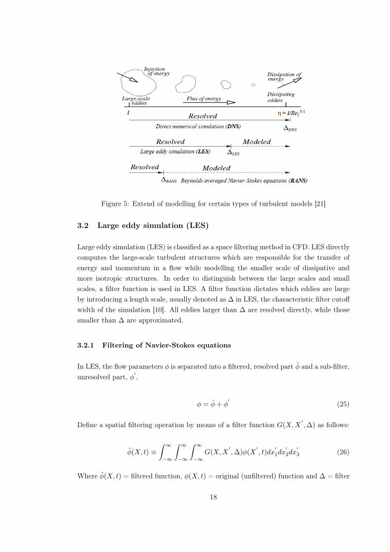
Figure 5: Extend of modelling for certain types of turbulent models [21]
3.2 Large eddy simulation (LES)
Large eddy simulation (LES) is classified as a space filtering method in CFD. LES directlycomputes the large-scale turbulent structures which are responsible for the transfer ofenergy and momentum in a flow while modelling the smaller scale of dissipative andmore isotropic structures. In order to distinguish between the large scales and smallscales, a filter function is used in LES. A filter function dictates which eddies are largeby introducing a length scale, usually denoted as ∆ in LES, the characteristic filter cutoffwidth of the simulation [10]. All eddies larger than ∆ are resolved directly, while thosesmaller than ∆ are approximated.
3.2.1 Filtering of Navier-Stokes equations
In LES, the flow parameters φ is separated into a filtered, resolved part φ and a sub-filter,unresolved part, φ′ ,
φ = φ+ φ′
(25)
Define a spatial filtering operation by means of a filter function G(X,X′,∆) as follows:
φ(X, t) ≡∫ ∞−∞
∫ ∞−∞
∫ ∞−∞
G(X,X′,∆)φ(X
′, t)dx
′1dx
′2dx
′3 (26)
Where φ(X, t) = filtered function, φ(X, t) = original (unfiltered) function and ∆ = filter
18

cutoff widthHere, the overbar indicates spatial filtering, not time-averaging. Equation (26) showsthat filtering is an integration,just like time-averaging in the development of the RANSequations, only in the LES the integration is not carried out in time but in three-dimensional space [1].
As mentioned, the filter function dictates the large and small eddies in the flow. Thisis done by the localized function G(X,X
′,∆). This function determines the size of the
small scales
G(X,X′,∆) =
{1/∆3 ‖X −X ′‖ ≤ ∆/20 ‖X −X ′‖ > ∆/2
(27)
Various filtering methods exist, the top-hat filter is common in LES. The function repre-sents Eq. (27). The top-hat filter is used in finite volume implementations of LES. Thecutoff width is intended as an indicative measure of the size of eddies that are retainedin the computations and the eddies that are rejected. In CFD computations with thefinite volume method it is pointless to select a cutoff width that is smaller than the gridsize. The most common selection is to take the cutoff width to be of the same order asthe grid size. In three-dimensional computations with grid cells of different length ∆x,width ∆y and height ∆z the cutoff width is often taken to be the cube root of the gridcell volume,
∆ = 3√
∆x∆y∆z (28)
Now, the unsteady Navier-Stokes equations for a fluid with constant viscosity µ are asfollows:
∂ρ
∂t+ div(ρu) = 0 (29)
∂(ρu)∂t
+ div(ρuu) = −∂p∂x
+ µdiv(grad(u)) + Su (30)
∂(ρv)∂t
+ div(ρvu) = −∂p∂y
+ µdiv(grad(v)) + Sv (31)
∂(ρw)∂t
+ div(ρwu) = −∂p∂z
+ µdiv(grad(w)) + Sw (32)
If the flow is also incompressible we have div(u) = 0, and hence the viscous momentumsource terms Su, Sv and Sw are zero.Filtering of above equations,
∂ρ
∂t+ div(ρu) = 0 (33)
19

∂(ρu)∂t
+ div(ρuu) = −∂p∂x
+ µ div(grad(u)) (34)
∂(ρv)∂t
+ div(ρvu) = −∂p∂y
+ µ div(grad(v)) (35)
∂(ρw)∂t
+ div(ρwu) = −∂p∂z
+ µ div(grad(w)) (36)
This equation set should be solved to yield the filtered velocity field u, v and w andfiltered pressure field p. We need to compute convective terms of the form div(ρφu)on the left hand side, but we only have available the filtered velocity field u, v, w andpressure field p [1]. To make some progress we write,
div(ρφu) = div(φu) + (div(ρφu)− div(φu))
The first term on the right hand side can be calculated from the filtered φ and u fieldsand the second term is replaced by a model. Substitution into above equation and somerearrangement yields the LES momentum equations:
∂(ρu)∂t
+ div(ρuu) = −∂p∂x
+ µ div(grad(u))− (div(ρuu)− div(uu)) (37)
∂(ρv)∂t
+ div(ρvu) = −∂p∂y
+ µ div(grad(v))− (div(ρvu)− div(vu)) (38)
∂(ρw)∂t
+ div(ρwu) = −∂p∂z
+ µ div(grad(w))− (div(ρwu)− div(wu)) (39)
In these equations, the first two terms on the left hand side denote the rate of changeand convective fluxes of filtered x−, y− and z−momentum. And third and forth termson the right hand side denote the gradients in the x−, y− and z−directions and diffusivefluxes of filtered x−, y− and z−momentum. The last terms are caused by the filteredoperation. They can be considered as a divergence of a set of stresses τij . In suffixnotation the i−component of these terms can be written as follows:
div(ρuiu− divρuiu) =∂(ρuiu− ρuiu)
∂x+∂(ρuiv − ρuiv)
∂y
+∂(ρuiw − ρuiw)
∂z=∂τij∂xj
(40)
20

Where τij = ρuiu− ρuiu = ρuiuj − ρuiuj (41)
The term τij is known as the subgrid scale (SGS) Reynolds Stress. Physically, the righthand side of Eq. (41) represents the large scale momentum flux due to turbulence motion.The nature of these contributions can be determined with the aid of a decomposition ofa flow variable φ(x, t) as the sum of (i) the filtered function ¯φ(x, t) and (ii) φ′
(x, t).
φ(x, t) = ¯φ(x, t) + φ′(x, t) (42)
Using this decomposition in Eq. (41) we can write the SGS stresses as follows:
τij = ρuiuj − ρuiuj = (ρuiuj − ρuiuj) + ρuiu′j + ρu
′iuj + ρu
′iu
′j (43)
thus, we find that the SGS stresses contain three groups of contributions:
• Leonard stresses Lij : Lij = ρuiuj − ρuiuj which represent the interactionbetween two resolved scale eddies to produce small scale turbulence.
• cross-stresses Cij : Cij = ρuiu′j+ρu
′iuj are the cross-stress terms that describe
the interaction between resolved eddies and small-scale eddies.
• LES Reynolds stresses Rij : Rij = ρu′iu
′j is the subgrid scale stress that
represents the interactions between two small scale eddies
3.2.2 Smagorinksy-Lilly SGS model
To approximate the SGS Reynolds stress, a SGS model can be employed. The mostcommonly used SGS models in LES is the Smagorinsky-Lilly model. In a flow, it isthe shear stress and the viscosity of the flow that cause the chaotic and random natureof the fluid motion. Thus, in the Smagorinsky-Lilly model, the effects of turbulenceare represented by the eddy viscosity based on the well known Boussinesq hypothesis.The Boussinesq hypothesis relates the Reynolds stress to the velocity gradients andthe turbulent viscosity of the flow [8]. It is therefore assumed that the SGS Reynoldsstress Rij is proportional to the modulus of the strain rate tensor of the resolved flowSij = 1
2(∂ui/∂xj + ∂uj/∂xi)
Rij = −2µSGSSij +13Riiδij = −µSGS
(∂ui∂xj
+∂uj∂xi
)+
13Riiδij (44)
where µSGS is the SGS eddy viscosity. Leonard stresses and cross-stresses are lumpedtogether with the LES reynolds stresses in the current versions of the finite volume
21

method. The whole stress τij is modeled as a single entity by means of a single SGSturbulence model.
τij = −2µSGSSij +13τiiδij = −µSGS
(∂ui∂xj
+∂uj∂xi
)+
13Riiδij (45)
The Smagorinksy-Lilly SGS model builds on Prandtl’s mixing length model and assumesthat we can define a kinematic SGS viscosity νSGS , which can be described in terms of theone length scale and one velocity scale and is related SGS viscosity by νSGS = µSGS/ρ.Since the size of the SGS eddies is determined by the details of the filtering function,the obvious choice for the length scale is the filter cutoff width ∆. The velocity scale isexpressed as the product of the length scale ∆ and the average strain rate of the resolvedflow ∆× ‖S‖, where ‖S‖ =
√2SijSij . Thus, the SGS viscosity is evaluated as follows:
µSGS = ρ(CSGS∆)2‖S‖ = ρ(CSGS∆)2√
2SijSij (46)
Where CSGS = constants and Sij = 12
(∂ui∂xj
+ ∂uj
∂xi
)where CSGS is the Smagorinsky constant that changes depending on the type of flow.For isotropic turbulent flow, the CSGS value is usually around 0.17 to 0.21. Basically, theSmagorinsky SGS model simulates the energy transfer between the large and the subgrid-scale eddies. Energy is transferred from the large to the small scales but backscattersometimes occurs where flow becomes highly anisotropic, usually near to the wall [4]. Toaccount for backscattering, the length scale of the flow can be modified using Van Driestdamping, and suggested that CSGS = 0.1 is most appropriate for this type of internalflow calculation.
The Smagorinksy model has been successfully applied to various flows as it is relativelystable and demands less computational resources among the SGS models. But somedisadvantages of the model have been reported,
• Too dissipative in laminar regions.
• Requires special near wall treatment and laminar turbulent transition.
• CSGS is not uniquely defined.
• Backscatter of flow is not properly modelled
Germano and Lilly conceived a procedure in which the Smagorinsky model constant,CSGS , is dynamically computed based on the information provided by the resolved scalesof motion. Hence, the dynamic SGS model has been introduced. This model employs a
22

similar concept as the Smagorinsky model, with the Smagorinsky constant CSGS replacedby the dynamic parameter Cdym [8]. The parameter Cdym is computed locally as afunction of time and space, which automatically eliminates the problem of using constantCSGS . In the dynamic SGS model, another filter is introduced which takes into accountof the energy transfer in the dissipation range. Performing the double filtering allowsthe subgrid coefficient to be calculated locally based on the energy drain in the smallestscales. Generally, the dynamic model predicted better agreement with experimentalwork in region of transition flow and the near wall region.
Some advantages of the dynamic model over the Smagorinsky-Lilly models are,
• Dynamic SGS automatically uses a smaller model parameter in isotropic flows.
• Near the wall, the model parameters need to be reduced; the dynamic SGS modeladapts these parameters accordingly.
3.3 Reynolds-averaged Navier-Stokes equations
The basic tool required for the derivation of the Reynolds-averaged Navier-stokes (RANS)equations from the instantaneous Navier–Stokes equations is the Reynolds decomposi-tion. Reynolds decomposition refers to separation of the flow variable into the meancomponent and the fluctuating component[1]. The following rules will be useful whilederiving the RANS equation. We begin by summarising the rules which govern timeaverages of fluctuating properties φ = Φ + φ and ψ = Ψ + ψ and their summation,derivatives and integrals:
φ′ = ψ′ = 0 Φ = φ∂φ
∂s=∂Φ∂s
∫φds =
∫Φds
φ+ ψ = Φ + Ψ φψ = ΦΨ + φ′ψ′ φΨ = ΦΨ φ′Ψ = 0 (47)
In addition, div and grad are both differentiations, the above rules can be extended toa fluctuating vector quantity a = A + a and its combinations with a fluctuating scalarφ = Φ + φ:
div a = div A; div(φa) = div(φa) = div(ΦA) + div(φ′a′);
div grad φ = div grad Φ (48)
Now, we consider the instantaneous continuity and Navier-Stokes equations in a Carte-sian co-ordinate system so that the velocity vector u has x-component u, y-componentv and z-component w:
23

div u = 0 (49)
∂u
∂t+ div(uu) = −1
ρ
∂p
∂x+ µdiv(grad(u)) (50)
∂v
∂t+ div(vu) = −1
ρ
∂p
∂y+ µdiv(grad(v)) (51)
∂w
∂t+ div(wu) = −1
ρ
∂p
∂z+ µdiv(grad(w)) (52)
This system of equations governs every turbulent flow, but we investigate the effectsof fluctuations on the mean flow using the Reynolds decomposition in equations (49),(50), (51) and (52) and replace the flow variables u and p by the sum of a mean andfluctuating component. Thus
u = U + u′
u = U + u′
v = V + v′
w = W + w′
p = P + p′
Then the time average is taken, applying the rules stated in equations (47) and (48).Considering the continuity equation (49), first we note that div u = div U. This yieldsthe continuity equation for the mean flow:
divU = 0 (53)
A similar process is applied on the x-momentum equation (50). The time averages ofthe individual terms in this equation can be written as follows:
∂u
∂t=∂U
∂tdiv(uu) = div(UU) + div(u′v′)
−1ρ
∂p
∂x= −1
ρ
∂p
∂xν div(grad(u)) = ν div(grad(U))
Substitution of these results gives the time-average x-momentum equation
∂U
∂t+ div(UU) + div(u′u′) = −1
ρ
∂P
∂x+ ν div(grad(U)) (54)
Repetition of this process on equations (51) and (52) yield the time-average y- andz-momentum equations:
24

∂V
∂t+ div(VU) + div(v′u′) = −1
ρ
∂P
∂y+ ν div(grad(V )) (55)
∂W
∂t+ div(WU) + div(w′u′) = −1
ρ
∂P
∂z+ ν div(grad(W )) (56)
Note that the terms (I), (II), (IV) and (V) in equations (54), (55) and (56) also appearin the instantaneous equations (50), (51) and (52), but the process of time averaging hasintroduced new terms (III) in the resulting time-average momentum equations [1]. Thisterms is product of fluctuating velocities and are associated with convective momentumtransfer due to turbulent eddies. And put these terms on the right hand side of equations(54), (55) and (56) to reflect their role as additional turbulent stresses on the meanvelocity components U, V and W:
∂U
∂t+ div(UU) = −1
ρ
∂P
∂x+ ν div (grad(U))
+1ρ
[∂(−ρu′2)
∂x+∂(−ρu′v′)
∂y+∂(−ρu′w′)
∂z
](57)
∂V
∂t+ div(VU) = −1
ρ
∂P
∂y+ ν div (grad(V ))
+1ρ
[∂(−ρu′v′)
∂x+∂(−ρv′2)
∂y+∂(−ρv′w′)
∂z
](58)
∂W
∂t+ div(WU) = −1
ρ
∂P
∂z+ ν div (grad(W ))
+1ρ
[∂(−ρu′w′)
∂x+∂(−ρv′w′)
∂y+∂(−ρw′2)
∂z
](59)
The extra stress terms have been written out as follows. They result from six additionalstresses among of three normal stresses
τxx = −ρu′2 τyy = −ρv′2 τzz = −ρw′2 (60)
and three shear stresses
τxy = τyx = −ρu′v′ τxz = τzx = −ρu′w′ τyz = τzy = −ρv′w′ (61)
These extra turbulent stresses are called the Reynolds stresses. The normal stressesinvolve the respective variances of the x-, y- and z-velocity fluctuations.They are always
25

non-zero because they contain squared velocity fluctuations [4]. The shear stresses con-tain second moments associated with correlations between different velocity components[4]. If two fluctuations velocity components, e.g. u
′ and v′ , are independent random
fluctuations the time average u′v′ would be zero. The equation set (53), (57), (58) and(59) is called the Reynolds-averaged Navier-stokes equations.
3.3.1 Standard κ− ε model
The Standard κ−ε (Launder and Spalding, 1974) model is the most widely used completeRANS model and it is incorporated in most commercial CFD codes [14]. In this model,the model transport equations are solved for two turbulence quantities i.e, κ and ε.The κ − ε turbulence model solves the flow based on the assumption that the rate ofproduction and dissipation of turbulent flows are in near-balance in energy transfer [19].We use κ and ε to define velocity scale ϑ and length scale ` representative of the largescale turbulence as follow:
ϑ = κ1/2 ` =κ3/2
ε
where κ is turbulent kinetic energy and ε is the dissipation of turbulent kinetic energy.This is then related to the turbulent viscosity µt based on the Prandtl mixing lengthmodel,
µt = Cρϑ` = ρCµκ2
ε(62)
where Cµ is a dimensionless constant and ρ is density of the flow.
The governing transport equations for κ and ε of the standard κ− ε model as follow,
∂(ρκ)∂t
+ div(ρκU) = div[µtσκ
grad κ]
+ 2µtSij .Sij − ρε (63)
∂(ρε)∂t
+ div(ρεU) = div[µtσε
grad ε]
+ C1εε
κ2µtSij .Sij − C2ερ
ε2
κ(64)
[I] [II] [III] [IV] [V]
where term [I] denotes the rate of change of κ or ε. In addition, term [II] and term [III]display the transport of κ or ε by convection and diffusion respectively [1]. Last twoterms describe the rate of production and destruction of κ or ε respectively.
Physically, the rate of change of kinetic energy in [I] in Eq.(63) is related to the convectionand diffusion of the mean motion of the flow. The diffusion term can be modelled bythe gradient diffusion assumption as turbulent momentum transport is assumed to be
26
proportional to mean gradients of velocity. The production term, which is responsiblefor the transfer of energy from the mean flow to the turbulence, is counterbalanced bythe interaction of the Reynolds stresses and mean velocity gradient. The destructionterm deals with the dissipation of energy into heat due to viscous nature of the flow[18].
The equations contains five adjustable constants: Cµ, σκ, σε, C1ε and C2ε. Based onextensive examination of a wide range of turbulent flows, the constant parameters usedin the equations take the following values,
Cµ = 0.09; σκ = 1.00; σε = 1.30; C1ε = 1.44 and C2ε = 1.92 (65)
where Prandtl numbers σκ and σε connects to diffusivities of κ and ε to the eddy viscosityµt.
The standard κ − ε model has gained popularity among RANS models due to thefollowing[8]:
• Robust formulation
• One of the earliest two-equation models, widely documented, reliable and affordable
• Lower computational overhead
• Excellent performance for many industrially relevant flows.
However, the model encounters some difficulties in:
• Fails to resolve flows with large strains such as swirling flows and curved boundarylayers flow
• Poor performance in rotating flows
3.3.2 Standard κ− ω model
Wilcox (1988) developed the standard κ − ω two equation model. The standard κ − ωmodel is very similar in structure to the κ − ε model but the variable ε is replaced bythe dissipation rate per unit kinetic energy, ω. If we use this variable the length scale is` =√κ/ω [4]. The eddy viscosity is given as follow,
µt = ρκ/ω (66)
The transport equations for κ and ω in standard κ− ω model are
27

∂(ρκ)∂t
+ div(ρκU) = div[(µ+
µtσκ
)grad (κ)
]+ Pκ − β∗ρκω (67)
[I] [II] [III] [IV] [V]
where Pκ =(
2µtSij .Sij − 23 ρκ
∂Ui∂xj
δij
)∂(ρω)∂t
+ div(ρωU) = div[(µ+
µtσω
)grad (ω)
]+ γ1Pω − β1ρω
2 (68)
[I] [II] [III] [IV] [V]
where Pω =(
2ρSij .Sij − 23 ρω
∂Ui∂xj
δij
)where term [I] denotes the rate of change of κ or ω in the both Eq.(67) and Eq.(68). Inaddition, term [II] and term [III] display the transport of κ or ω by convection and diffu-sion respectively [4]. Terms [IV] and [V] describe the rate of production and destructionof κ or ω respectively.
The model constants are as follow,
σκ = 2.0; σω = 2.0; γ1 = 0.553; β1 = 0.075 and β∗ = 0.09 (69)
The replacement with the variable ω allows better treatment in solving the flow nearwall. Near to the wall, the boundary layer is affected by viscous nature of the flow. Avery refined mesh is necessary to appropriately resolve the flow [8]. Although the nearwall treatment of standard κ − ε model saves a vast amount of computer power, it isnot sufficient to represent complex flow accurately. In the standard κ − ω formulation,the flow near wall is resolved directly through the integration of the ω equation. Theadvantage of the standard κ−ω model compared to the standard κ− ε model is that theω equation is more robust and easier to integrate compared to the ε equation withoutthe need of additional damping functions.
3.3.3 Shear-Stress Transport (SST) κ− ω model
The shear-stress transport (SST) κ − ω model was developed by Menter (1994) to ef-fectively blend the robust and accurate formulation of the κ− ω model in the near-wallregion with the free-stream independence of the κ− ε model in the far field. To achievethis, the κ− ε model is converted into a κ− ω formulation [8]. The SST κ− ω model issimilar to the standard κ− ω model, but includes the following refinements:
28

• The standard κ−ω model and the transformed κ− ε model are both multiplied bya blending function and both models are added together. The blending functionis designed to be one in the near-wall region, which activates the standard κ − ωmodel, and zero away from the surface, which activates the transformed κ − ε
model.
• The SST model incorporates a damped cross-diffusion derivative term in the ωequation.
• The definition of the turbulent viscosity is modified to account for the transportof the turbulent shear stress.
• The modeling constants are different.
The Reynolds stress computational and the κ equation are the same as in standard κ−ωmodel, but the ε equation transformed into an ω equation by substituting ε = κω. Thisyields
∂(ρω)∂t
+ div(ρωU) = div[(µ+
µtσω,1
)grad (ω)
]+
γ2
(2ρSij .Sij −
23ρω
∂Ui∂xj
δij
)− β2ρω
2 + 2ρ
σω,2ω
∂κ
∂xκ
∂ω
∂xκ(70)
In the above equation all terms are same as in ω equation (68) in standard κ− ω modelexcepted last term. The last term is called the cross-diffusion term, which arises duringthe ε = κω transformation of the diffusion term in the ε equation [1].
The model constants are as follow,
σκ = 1.0; σω,1 = 2.0; σω,2 = 1.17; γ2 = 0.44; β2 = 0.083 and β∗ = 0.09 (71)
Here, blending functions are used to achieve a smooth transition between standard κ−ωand transformed κ − ε models. Blending functions are introduced in the equation tomodify the cross-diffusion term and are also used for model constants that take value C1
for the original κ− ω model and value C2 in Menter’s transformed κ− ε model.
C = FcC1 + (1− Fc)C2 (72)
Where Fc is blending function. The functional form of Fc is chosen so that it (i) is zero atthe wall (ii) tends to unity in the far field and (iii) produces a smooth transition arounda distance half way between the wall and edge of the boundary layer [1].
The SST κ− ω model more accurate and reliable for a wider class of flows like, adversepressure gradient flows, airfoils, transonic shock waves than the standard κ− ω model.
29

3.4 The law of the wall
Turbulent flows are significantly affected by the presence of walls. Obviously, the meanvelocity field is affected through the no-slip condition that has to be satisfied at the wall.However, the turbulence is also changed by the presence of the wall in non-trivial ways.close to the wall the flow is influenced by viscous effects and does not depend on freestream parameters. the mean flow velocity only depends on the distance y from the wall,fluid density ρ and viscosity µ and the wall shear stress τw [4]. So
U = f(y, ρ, µ, τw)
Dimensional analysis shows that
u+ =U
uτ= f
(ρµτy
µ
)= f(y+) (73)
Formula Eq. (73) is called the law of the wall and contains the definitions of two impor-tant dimensionless groups, u+ and y+. Here uτ =
√τw/ρ is called friction velocity.
The κ − ε models, the RSM, and the LES model are primarily valid for turbulent coreflows and will not predict correct near-wall behavior if integrated down to the wall.Therefore, it is necessary to make these models suitable for wall-bounded flows. TheSpalart-Allmaras and κ−ω models were designed to be applied throughout the boundarylayer, provided that the near-wall mesh resolution is sufficient.
Numerous experiments have shown that the near-wall region can be largely subdividedinto three layers.
1. Linear or viscous sub-layer:- the fluid layer in contact with a smooth wallAt the solid surface the fluid is stationary. Turbulent eddying motions must stop veryclose to the wall and the behavior of the fluid closest to the wall is dominated by viscouseffects. The viscous sub-layer is in practice extremely thin (y+ < 5) and assume thatthe shear stress is approximately constant and equal to the wall shear stress τw. Aftersome simple algebra and making use of the definitions of u+ and y+ this lead to
u+ = y+ (74)
Because of the linear relationship between velocity and distance from the wall the fluidlayer adjacent to the wall is also known as the linear sub-layer.
2. Log-law layer:- the turbulent region close to a smooth wallOutside the viscous sublayer a region exists where viscous and turbulent effects areboth importance. The shear stress τ varies slowly with distance from the wall [4]. and
30

within this inner region it is assumed to be constant and equal to the wall shear stress.Relationship between u+ and y+ that is dimensionally correct:
u+ =1kln(y+) +B =
1kln(Ey+) (75)
Here, von karman’s constant k = 0.4 and the additive constant B = 5.5 or ( E = 9.8)for smooth wall, wall roughness cause a decrease in the value of B. The value of k and Bare universal constants valid for all turbulent flows past smooth walls at high Reynoldsnumber. Formula (75) is often called the log-law, and the layer where y+ takes valuesbetween 30 and 500 the log-law layer.
3. outer layer:- the inertia-dominated region far from the wallExperimental measurements show that the log-law is valid in the region 0.02 < y/δ < 0.2.For larger values of y the velocity-defect law provides the correct form [8]. In the overlapregion the log-law and velocity-defect law have to equal and overlap is obtained byassuming the following logarithmic form:
Umax − Uut
= −1kln(yδ
)+A (76)
Where A is a constant. The velocity-defect law is often called the law of the wake.
Figure 6: Subdivisions of the Near-Wall Region [8]
From Fig.6 we can say that the turbulent boundary layer adjacent to a solid surface iscomposed of two regions [1]:
• The inner region: 10− 20% of the total thickness of the wall layer; the shear stress
31

is constant and equal to the wall shear stress τw. Within this region there are threezones.
1. the linear sub-layer: viscous stresses dominate the flow adjacent to surface.
2. the buffer layer: viscous and turbulent stresses are of similar magnitude.
3. the log-law layer: turbulent stresses dominate.
• The outer region or law-of-the-wake layer: inertia-dominated core flow far fromwall; free from direct viscous effects.
32

4 Flow past a circular cylinder
Flow past a circular cylinder has been the subject of both experimental and numericalstudies for decades. This flow is very sensitive to the changes of Reynolds number, adimensionless parameter representing the ratio of inertia force to viscous force in a flow.Work in this chapter aims to validate and identify suitable turbulence models in theapplication of the flow past a circular cylinder. Flow around a circular cylinder has beenchosen as pilot study for the investigation on the flow around a bridge deck section dueto the effect of vortex shedding on such structures. To begin with, the basic overviewof the flow around a circular cylinder and the flow characteristics such as the Strouhalnumber, vortex shedding, drag, lift, and pressure coefficients are introduced.
4.1 Conceptual overview of flow past a circular cylinder
Flow past a circular cylinder tends to follow the shape of the body provided that thevelocity of the flow is very slow, this is known as laminar flow. Flow at the inner partof the boundary layers travels more slowly than the flow near to the free stream. As thespeed of the flow increases, separation of flow occurs at some point along the circularcylinder due to the occurrence of the adverse pressure gradient region . Flow separationtends to roll up the flow into swirling eddies, resulting in alternate shedding of vorticesin the wake region of the body known as the von Karman vortex street.
4.1.1 Reynolds number
Flow past a circular cylinder varies with the Reynolds number. Small Reynolds numbercorresponds to slow viscous flow where frictional forces are dominant. When Reynoldsnumber increases, flows are characterised by rapid regions of velocity variation and theoccurrence of vortices and turbulence. Mathematically, Reynolds number of the flowaround a circular cylinder is represented by,
Re =ρuD
µ(77)
where D is the diameter of the cylinder, u is the inlet velocity of the flow, ρ is a densityof fluid and µ is the dynamic viscosity of fluid.Experimental study of the flow around a circular cylinder has identified regions wheresignificant patterns of flow occur as the Reynolds number changes, especially when theflow changes from laminar to turbulent state. Generally, the following regimes have beenidentified from experiment [7]:
33

Stable range 40 < Re < 150
Transition range 150 < Re < 300
Irregular range 300 < Re < 200, 000
Flow becomes very irregular with instabilities beyond Reynolds number of 200,000. An-other dominant feature of the flow around a circular cylinder is the three-dimensionalnature of the flow. Bloor (1964) [11] investigated the flow around a circular cylinderbetween Reynolds number of 200 to 400 when turbulent motion starts to develop in thewake region of the flow. He observed that the transition of flow in the wake region istriggered by large-scale three-dimensional structures.
4.1.2 Vortex shedding and Strouhal number
The separation of flow past a circular cylinder causes pairs of eddies to form alternatelyon the top and bottom part of the cylinder and travel into the wake region resulting invortex shedding. Vortex shedding is very common in engineering applications. Figure7 shows vortex shedding phenomenon in the wake region of the flow past a circularcylinder. Laminar vortex shedding known as the von Karman vortex street has beenobserved in the wake region of the flow past a circular cylinder at low Reynolds numberbetween 40 to 250. For Reynolds number that is greater than 250, the laminar periodicwake becomes unstable and the eddies start to become turbulent. Further increase ofReynolds number turns the wake region into turbulent flow. Within certain range ofReynolds number (250 < Re < 10,000), the frequency at which vortices are shed in theflow around a circular cylinder tends to remain almost constant.
Figure 7: Vortex shedding in the wake region of the flow past a circular cylinder [31].
Strouhal number is a dimensionless parameter which describes the shedding of the vor-tices in the wake region of a flow. It relates the frequency of vortex shedding to theincident wind speed,
34

St =fsD
u(78)
where D is the diameter of the cylinder and u is the velocity of the flow. fs is theshedding frequency of vortices equal to 1/T and fs is called the Strouhal frequency orthe vortex shedding frequency where T denotes for period.
4.1.3 Drag, lift and pressure coefficients
The drag force acts in a direction that is opposite of the relative flow velocity (i.e.,it opposes the relative flow). It depends on shape and orientation of a body. Dragcoefficient, Cd is calculated as follow:
Cd =Fd
1/2ρu2A(79)
where A is the projected area in the flow direction and Fd is the sum of the pressureforce and the viscous force components on the cylinder surface acting in the horizontaldirection. Lift coefficient, Cl is calculated similarly but vertical force is considered ratherthan horizontal force which is shown in Figure 8.
Cl =Fl
1/2ρu2A(80)
The Strouhal number is related to the Cd of the flow. In sub-critical Reynolds numberregion (100 < Re < 10,000), increase in the Strouhal number is generally accompaniedby a decrease of the Cd.
Figure 8: Diagram of forces acting around a circular cylinder.
Theoretically, the drag force is changing at twice the frequency of the lift force for the flowpast a circular cylinder or generally flow involving separation. When a vortex is shed fromthe top of the cylinder, a suction area is created and the cylinder experiences lift. Half acycle later, an alternate vortex is created at the bottom part of the cylinder. Throughoutthe process, the lift force changes alternately in a complete cycle of vortex shedding but
35

the cylinder experiences drag constantly. It is important that any turbulence modelscan simulate all the forces coefficient correctly for the analysis of the flow past circularcylinder.
Apart from the Cd and Cl, the pressure coefficient, Cp, distribution around the surfaceof the cylinder is important. Near to the surface of the cylinder, flow momentum is quitelow due to viscous effects and thus is sensitive to the changes of the pressure gradient.Cp plot of the flow around a circular cylinder starting from the stagnation point (zerovelocity) where Cp takes a value of one according to Bernoulli’s Theorem. The flow speedthen starts to increase accompanied by a drop in the Cp to a negative value.
The speed of flow then starts to reduce near θ = 80◦, [7] along with an incrementof pressure in the direction of the flow, which results in the adverse pressure gradientsituation. The flow now has to move against the pressure force in addition to the viscousforce. This leads to a reduced gradient of the velocity profile and the wall shear stress.Separation of flow occurs when the shear stress cannot overcome the adverse pressuregradient, this usually happens at 80◦ < θ < 120◦ [7] for sub-critical flow. After theseparation point, pressure remains fairly constant in the wake. Accurate prediction ofCp distribution around a cylinder means a turbulence model performs well at predictingthe flow separation
4.2 Computational details
In the current work, RANS models such as the κ − ε model, the SST model and theLES model have been chosen to test the suitability and the applicability of the modelson the flow past a circular cylinder for Reynolds number of 1000 and 3900. In addition,we have studied the grid and time-step sensitivity using the RANS and the LES modelsfor Reynolds number of 1000. Also, experimental data such as the pressure distribution,drag coefficient and Strouhal number are widely available within these Reynolds numbersfor comparative study. The RANS models and the LES model used here employ a finitevolume method (FVM). The brief details of the simulations are as follows:
• Computational domain
The computational domain and the boundary conditions for the simulation of theflow are shown in Figure 9. The cylinder is simulated with a diameter (D) of 6 mmand a depth of πD to incorporate the spanwise effects. The computational domainconsists of an upstream of 10 times the diameter to downstream of 25 times thediameter of the cylinder and 8 times the diameter on each cross-stream direction.
36

Figure 9: Computational geometry and boundary conditions.
• Boundary conditions
Longitudinal uniform velocities of 0.0167 m/s and 0.0651 m/s are introduced atthe inlet correspond to the Reynolds number of 1000 and 3900 respectively. Theoutlet boundary is defined with an average static reference pressure of 0 Pa. Therest of the boundaries (side and bottom wall) and the cylinder wall are no slip wallboundary condition where velocity increases from zero at the wall surface to thefree stream velocity away from the surface.
• Meshing
A structured hexahedral mesh is employed in these simulations. Structured meshis generated using ANSYS GAMBIT 2.4, the grid generation component of AN-SYS Fluent 12.1, and then imported into ANSYS Fluent. Figure 10a displays themesh generation in the computational domain. Figure 10b shows the grid near thecylinder surface of the domain. Near to the cylinder wall and in the wake, veryfine mesh are required to resolve boundary layer separation and the vortex street.The 3D closer view of near the cylinder surface is shows in Figure 10c. Hexahedralcells form the grid structures around the cylinder. Furthermore, to fully resolvethe viscous sublayer, it is necessary to place at least a few cells within y+ < 5and to have y+ ≈ 1 for the first cell adjacent to the cylinder. To obtain reason-able mesh size for the computational procedure, this can be achieved by using ablockstructured grid. Accordingly, a block-structured mesh type is generated in arectangular domain.
37

Figure 10: (a) Computational domain, (b) grid around the cylinder, and (c) 3Dcloser view of the cylinder.
• Simulation set-up
The numerical solution of the flow is obtained using a commercial CFD code:ANSYS Fluent 12.1. In this 3D-code, discretization is done based on a finitevolume approach. In this section the various CFD code settings and options aresummarized. An unsteady and pressure based solver are used. A least square cellbased method is used to calculate gradients. Boundary conditions and differentdiscretization schemes are used depending on the turbulence model. They aresummarized in Table 1 and Table 2, for RANS models and for LES respectively.We have considered convergence criteria 1.0 × 10⁻⁵ for these simulations. Theboundary conditions for LES are same as mentioned in the Table 1.
38

Table 1: Simulation settings for flow past a circular cylinder case with RANS models
Settings Choice
Simulation type 3D, UnsteadySolver Double precision, Pres-
sure based and implicitTemporal discretization 2nd orderTurbulence model κ− ε and SST modelsPressure StandardPressure-velocity coupling SIMPLEMomentum 2nd order upwindTurbulent kinetic energy 2nd order upwindTurbulent dissipation rate 2nd order upwind(for κ− ε model)Specific dissipation rate 2nd order upwind(for SST model )
Boundary conditions:
Inlet Velocity inletOutlet Pressure outletTop wall No-slip wallBottom wall No-slip wallCylinder wall No-slip wall
Table 2: Simulation settings for flow past a circular cylinder case with LES model
Settings Choice
Simulation type 3D, UnsteadySolver Double precision, Pres-
sure based and implicitTemporal discretization 2nd orderPressure StandardPressure-velocity coupling SIMPLEMomentum Bounded Central differ-
encingSGS model Smagorinsky-Lilly
model, Dynamic stress
39

4.3 Results and Discussions
The simulations are conducted for two Reynolds numbers of 1000 and 3900, both ofwhich are in the sub-critical regime. The choice of the Reynolds numbers of simulationdepends largely on the experimental data available. It is known that the flow past thecylinder is two dimensional only when Re < 200. For large Reynolds numbers, thevortex shedding occurs in cells and therefore the flow is generally simulated in 3D [22].Therefore, all the simulations have been performed in transient and 3D. Critical flowparameters, which are non-dimensional vortex shedding frequency, time-averaged dragcoefficient and fluctuating lift coefficient, have been predicted with each turbulence modeland some of them calculated values are compared with experimental. In addition, time-averaged pressure distribution are calculated around the cylinder surface with mentionedturbulence models.
4.3.1 Discussion of the test case with ReD = 1000
In this section, we will discuss the cases with ReD = 1000. For this purpose, we havebeen used two different approaches namely, RANS models such as the κ− ε model, theSST model and the LES model. Here, all simulations have done using Grid B. Grid Bcontains 388550 cells. The detail information about it which is given in the Table 5.
The overall forces acting on the cylinder are important parameters for practical applica-tion of CFD. Table 3 presents experimental data alongside the mean drag, Cd, Strouhalnumber, St, and the angle of separation of the flow, θs, for each of the turbulence mod-els. Table shows that SST model computes drag coefficient, Cd accurately and it is closeto the experimental value. Where the κ − ε model and LES model give the Cd valuelittle bit high compare to SST model. The Strouhal number of the flow is calculatedbased on the oscillating frequency of the lift coefficient. The time domain data of thelift coefficient is converted into frequency domain by using the Fast Fourier Transform(FFT). The frequency of the lift coefficient fs is then substituted into Eq.(68) to get theStrouhal number. Good agreement with the experimental result is observed from LES.The value of separation angle, θs, is the non-dimensional pressure coefficient at the rearstagnation point. The angle of separation of the flow from LES is 79.5◦, close to theexperimental value of 65± 2◦. LES gives better result compare to the κ− ε model andSST model.
Figure 11 shows the first 25 seconds of the time history of the lift and drag coefficientspredicted by LES for the flow past a circular cylinder. From Figure 11b, we can see thatthe LES model gives good Cl value which is useful to find the strouhal number. Boththe κ − ε model and the SST model fail to predict the Cl of the flow around a circular
40

cylinder for sub-critical Reynold number. Therefore, the κ− ε and the SST models arevery poor to compute the strouhal number.
Table 3: Experimental and computational results for ReD = 1000
ReD = 1000Cd St θs
Exp 0.98± 0.005 0.21 65± 2κ− ε 1.1169 — 84SST 0.9891 — 82LES 1.1499 0.21 79.5
Figure 11: Time histories of (a) drag coefficient,Cd, and (b) lift coefficient, Cl, for LES.
41
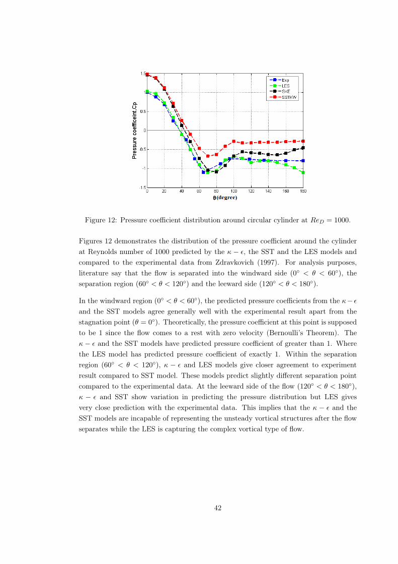
Figure 12: Pressure coefficient distribution around circular cylinder at ReD = 1000.
Figures 12 demonstrates the distribution of the pressure coefficient around the cylinderat Reynolds number of 1000 predicted by the κ − ε, the SST and the LES models andcompared to the experimental data from Zdravkovich (1997). For analysis purposes,literature say that the flow is separated into the windward side (0◦ < θ < 60◦), theseparation region (60◦ < θ < 120◦) and the leeward side (120◦ < θ < 180◦).
In the windward region (0◦ < θ < 60◦), the predicted pressure coefficients from the κ− εand the SST models agree generally well with the experimental result apart from thestagnation point (θ = 0◦). Theoretically, the pressure coefficient at this point is supposedto be 1 since the flow comes to a rest with zero velocity (Bernoulli’s Theorem). Theκ − ε and the SST models have predicted pressure coefficient of greater than 1. Wherethe LES model has predicted pressure coefficient of exactly 1. Within the separationregion (60◦ < θ < 120◦), κ − ε and LES models give closer agreement to experimentresult compared to SST model. These models predict slightly different separation pointcompared to the experimental data. At the leeward side of the flow (120◦ < θ < 180◦),κ − ε and SST show variation in predicting the pressure distribution but LES givesvery close prediction with the experimental data. This implies that the κ − ε and theSST models are incapable of representing the unsteady vortical structures after the flowseparates while the LES is capturing the complex vortical type of flow.
42

Figure 13: Iso-surfaces of x-vorticity produced from ske and SST models with ReD =1000.
Figure 14: Iso-surfaces of instantaneous x-vorticity with ReD = 1000.
43

Figure 15: Contours of velocity magnitude and velocity vector with ReD = 1000.
Figure 13 shows the formation of x-vorticity street predicted in the wake region of theflow past a circular cylinder using the κ− ε and the SST models at Reynolds number of1000 after 25 s. There are no any changes in these profiles with time. From Figure 13 itcan be seen that the RANS models are not able to capture the vortex shedding behindthe cylinder. Where Figure 14 demonstrates iso-surfaces of instantaneous x-vorticitywith ReD = 1000 using the LES model. It is shows the ability of the LES model topredict an unsteady motion in the wake region of the flow.
The vortex shedding is visualized by the velocity and its vector also. Contours of velocitymagnitude and velocity vector using LES at ReD = 1000 are shown in Figure 15. Figuredisplays velocity vector in the near field of the cylinder. From Figure 15, it can be seenthat the LES model able to separate the flow behind the cylinder.
44

4.3.2 Discussion of the test case with ReD = 3900
In this section, we will discuss the cases with ReD = 3900. We have been performed allthe simulations using Grid B which was used in the above case. Critical flow parameters,which are time-averaged drag coefficient, non-dimensional vortex shedding frequency andthe angle of separation of the flow, have been predicted with each turbulence model ( theκ−εmodel, the SST model and the LES model) and their calculated values are illustratedin Table 4. Table 4 shows that the experimental value of the Cd is 0.93± 0.005 [7]. theκ− ε model and the SST model are predicted the Cd value lower than the experimentalvalue and they are around 18% and 30% respectively. While the Cd obtained from theLES model is little bit higher than the experimental and it is around 13%. From Table4, it can be clear that the LES model yield better the Cd value compared to the κ − εand the SST models for Reynolds number of 3900. The κ − ε model is fail to computethe Strouhal number while the SST model overestimates it for Reynolds number of 3900.The LES model is provide a closer match to the experimental value for the St. the valueof separation angle, θs, has good agreement with the experimental from the LES model.Where the κ− ε and the SST are also predict the θs close to the experimental value.
Table 4: Experimental and computational results for ReD = 3900
ReD = 3900Cd St θs
Exp 0.93± 0.005 0.215± 0.005 82± 2κ− ε 0.7446 — 85SST 0.6208 — 85LES 1.0683 0.20 81
Figure 16: Cl history for κ− ε and SST with ReD = 3900.
45

Figure 16 shows the time history of the lift coefficient predicted by the κ−ε and the SSTmodels for Reynolds number of 3900. From figure, it is clear that the κ− ε model is verypoor for to compute the Cl value for ReD = 3900. Where, the SST model gives the Clvalue for this Reynolds number, but it is not able to predict the Cl for ReD = 1000. Forthis reason, we can say that the SST model is good to compute the force coefficients forhigh Reynolds number. The SST model is much more recommendable for high Reynoldsnumber [22]. In addition, Figure 17 presents the effect on the time variation of drag andlift coefficients using the LES model for flow past a circular cylinder. These coefficientsare the standard normalization of the respective forces using the projected area and thedynamic pressure of the oncoming stream. Most obvious is the oscillation of the lifttraces – showing the effect of the periodic vortex shedding. Notice that the frequency ofthe drag oscillation is roughly twice the frequency of the lift coefficient.
Figure 17: Cd and Cl histories for LES with ReD = 3900.
46
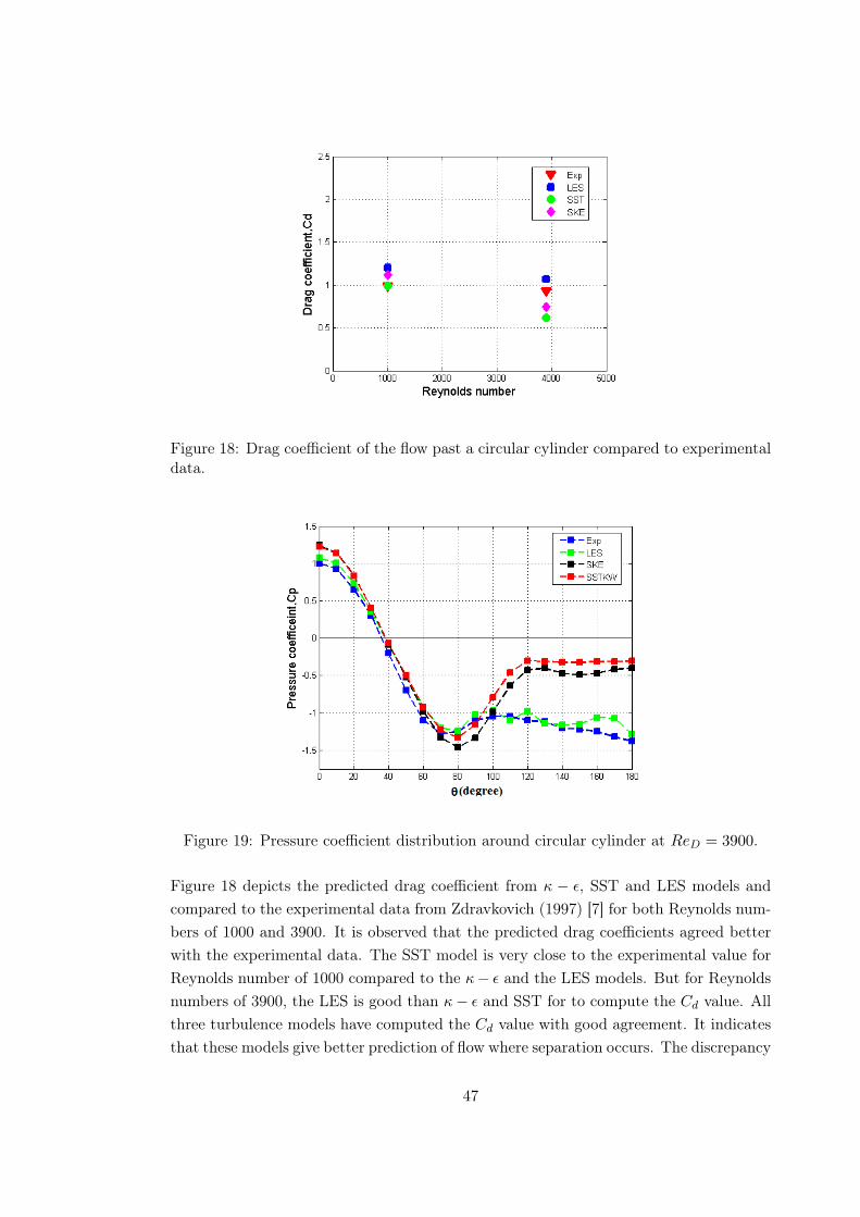
Figure 18: Drag coefficient of the flow past a circular cylinder compared to experimentaldata.
Figure 19: Pressure coefficient distribution around circular cylinder at ReD = 3900.
Figure 18 depicts the predicted drag coefficient from κ − ε, SST and LES models andcompared to the experimental data from Zdravkovich (1997) [7] for both Reynolds num-bers of 1000 and 3900. It is observed that the predicted drag coefficients agreed betterwith the experimental data. The SST model is very close to the experimental value forReynolds number of 1000 compared to the κ− ε and the LES models. But for Reynoldsnumbers of 3900, the LES is good than κ− ε and SST for to compute the Cd value. Allthree turbulence models have computed the Cd value with good agreement. It indicatesthat these models give better prediction of flow where separation occurs. The discrepancy
47

is caused by different base suction predicted near the leeward side (120◦ < θ < 180◦), ofthe cylinder. This can be seen from Figure 19, where a less negative pressure has beenpredicted, results in lower suction and thus lower drag around this area.
Figure 19 presents the distribution of the pressure coefficient around the cylinder atReynolds number of 3900 predicted by the κ − ε, the SST and the LES models whichare compared to the experimental data. In the windward region (0◦ < θ < 60◦), thepredicted pressure coefficients from the κ − ε and the SST models agree generally nicewith the experimental result expected the stagnation point (θ = 0◦). The κ− ε and theSST models have predicted pressure coefficient little bit more than 1 at (θ = 0◦). Wherethe LES model has predicted pressure coefficient of exactly 1 at (θ = 0◦) which is sameas the experimental value. Within the separation region (60◦ < θ < 120◦), all threeturbulence models give closer agreement to the experiment result. At the leeward side ofthe flow (120◦ < θ < 180◦), κ− ε and SST are failed to accurately predict the pressuredistribution after separation of the flow occurred with increasing pressure coefficientsobserved rather than a more constant behaviour as reported from experiment. The LESyields good agreement with the experiment result after separation of the flow.
Figure 20: Iso-surfaces of x-vorticity produced from ske and SST models with ReD =3900.
48

Figure 21: Iso-surfaces of instantaneous x-vorticity with ReD = 3900.
Figure 20 shows the iso-surface of x-vorticity have been predicted in the wake region ofthe flow past a circular cylinder using the κ− ε and the SST models at Reynolds numberof 3900. From Figure 20, it is clear that the κ − ε model is incapable of representingthe unsteady vortex shedding after the flow separation since it is not able to computethe Cl value and the Strouhal number. while the SST model is capturing the complexvortex shedding of flow. Figure 21 demonstrates iso-surfaces of instantaneous x-vorticityhas predicted by the LES model for ReD = 3900. In this figure, it can be seen that theLES successfully captured the main features of the wake structure of the cylinder. TheLES model predicts the unsteady complex vortex shedding in the wake region of the flowbehind the cylinder.
49

4.3.3 Grid sensitivity study with ReD = 1000
In view of the encouraging results obtained above with CFD simulations, we have at-tempted to investigate the influence of grid on critical flow parameters for flow past acircular cylinder. For the RANS turbulence models, the results remain almost constantwith increasing grid size from medium to fine mesh [23]. The LES approach to flowpast a circular cylinder is an expensive approach due to its demanding requests of com-putational time and accurate mesh generation. Due to this, in order to check the gridsensitivity, three different grids have been chosen. All simulations are performed with asame time-step (∆t = 0.001). For the RANS models, the drag coefficient, Cd, with threedifferent grids have been calculated. In addition, we have studied all flow parameters,which are time-averaged drag coefficient, Strouhal number and the angle of separationof the flow using the LES model with various mesh.
The brief details about grids are listed in the Table 5. Table provides some details ofthe grids, including the total number of nodes, the numbers of nodes in the x-, y- andz-directions, and y+ characteristics of each grid. The number of elements employedin the simulations are 152880, 388550 and 486200 for Grid A, B and C respectively.Furthermore, here Nx, Ny and Nz display the number of nodes in the x-, y- and z-directions respectively. Table 5 shows maximum and minimum of y+ for all grids. It canbe seen that all of the meshes have considerably low y+ values to sufficiently resolve theviscous sublayer.
Table 5: Details of grids used in mesh-independence tests
Grid Cell size Nx Ny Nz Max.y+ Min.y+ Ave.y+
A 152880 148 75 12 12 1.0 5.5
B 388550 190 90 19 9.5 0.8 4.35
C 486200 190 100 22 9.0 0.7 4.15
Table 6 shows the changes of the drag coefficient predicted by the κ − ε and the SSTmodels with simulations of different meshes and order of accuracy. The SST model givesgood agreement with the experiment result for all three grids, compared to the κ − εmodel. The κ − ε model yields little bit higher Cd value than the experiment result.From table it is clear that the both models are predicted the Cd values almost same forGrid B and Grid C. As it can be seen, the results remain almost constant with increasing
50

grid size from Grid B to Grid C. Thus, one can conclude that incremental grid size isnot necessary for the RANS models, and the Grid B is sufficiently fine for to computethe better Cd value.
Table 6: Drag coefficient of the flow past a circular cylinder using the RANS models
ReD = 1000Grid Cd(Exp.) Cd
A 0.98± 0.005 1.0245κ− ε B 0.98± 0.005 1.1169
C 0.98± 0.005 1.1199A 0.98± 0.005 0.8538
SST B 0.98± 0.005 0.9891C 0.98± 0.005 0.9816
Amesh sensitivity analysis has been conducted for the LES of flow past a circular cylinderat Reynolds number of 1000. Three mesh types, LES 1 with Grid A, LES 2 with GridB and LES 3 with Grid C have been compared. Table 7 presents the experimental dataalonside the Cd, the Strouhal number and the angle of separation of the flow for each gridof the CFD cases. The LES 3 predicts the Cd value which is good compared to LES 1 andLES 2, and it is close to the experimental value. LES 1 and LES 2 give the Cd value higherthan the experimental and they are more around 20% and 16% respectively. All gridsdemonstrate same value of the Strouhal number, which are identical to the experimentaldata. All three LES models are provided the θs value. The value of separation angle,θs, has good agreement with the experimental from LES 3. We can clearly observe thatthere is very little variation in the θs value when we refine the grid from Grid B to GridC. By using these grids, we have investigated that the influence of grid refinement on theCd value and the θs value. Table 7 demonstrates that the Strouhal number is insensitiveto any further grid refinement.
Table 7: Computed flow parameters in comparison with experimental results using LES
ReD = 1000Grid Cd St θs
Exp — 0.98± 0.005 0.21 65± 2LES1 A 1.1811 0.21 82LES2 B 1.1499 0.21 79.5LES3 C 1.0542 0.21 78
51

Figure 22: Cd and Cl histories with different grids for LES.
Figure 22a and b present the evolution of the drag and lift coefficients for the LES casesusing different grids respectively. It is clear from Figure 22a, Grid A has high oscillationwhile Grid B and C produce lower frequency compared to Grid A. Figure 22b shows thatthe amplitude of lift oscillation decrease with grid from Grid A to Grid C.
52

Figure 23: Iso-surface of the magnitude of instantaneous vorticity for LES with (a) GridA, (b) Grid B, and (c) Grid C.
Note that Nz (number of grid point in the z-direction) will effect on the vortex sheddingin the wake region of the flow past a circular cylinder. Figure 23a, b and c present iso-surface of the magnitude of instantaneous vorticity for each of LES cases. From Figure23a, it is clear that Grid A is poor to capture the three-dimensional vortical structuresbehind the cylinder. It has an evidence that it is fail to predict some smaller scale eddiesand the reduction in the strength of the vorticity as the flow moves downstream. Figure23b and c show that Grid B and C have ability to produce complex vortical type of flowbehind the cylinder. Moreover, both have quite similar vortex shedding profiles. So, wecan say that grid has influence on vortex shedding and grid A is not able to capture smalldetails of the flow while Grid B and C have not significant effect on the vortex street inthe wake region of the flow past a circular cylinder. Figure 24a, b and c demonstratecontours of x-velocity predicted by LES with different grids. In figure, the blue area
53

shows the wake field with negative velocity. It can be seen from figure, Grid B and Cgive good details about flow field compared to Grid A.
Figure 24: Contour of x-velocity for LES with (a) Grid A, (b) Grid B, and (c) Grid C.
Computational time
Transient calculation in CFD is highly depends on computational power. Grid size isthe most important parameter which effect on the CPU time. Moreover, CPU time isdepended on choice of turbulence models also. To perform all the transient simulations,we have used 1 ms time-step. For better convergence, we have fixed 10 iterations pertime-step. All the simulations of the present work were carried out with parallel com-puting with Intel Core2 Quad Q6600 2.4 GHz processor and 4 GB of RAM. FollowingTable 8 represents the details of the CPU time used by each models with selected grids.
54

Table contains the computational time required to simulate 25 second period.
Table 8: CPU times details used by each model for different grids.
Model Grid Total CPUTime(hrs)
A 63.03κ− ε B 120.00
C 182.67A 70.62
SST B 168.00C 261.28A 226.00
LES B 561.80C 685.24
Table shows that LES approach is quite expensive compared to RANS. For each model,CPU time increases with increment in the grid size.
4.3.4 Effect of time-step size with LES
This sub-section provides a study of the cylinder flow simulations performed at threedifferent time-steps. We have done all simulations using Grid B for the LES model. Thechoice of a smaller time step might be superfluous in certain points of the flow. Also,the numerical grid will most probably not be fine enough to simulate the length scaleswhich correspond to the micro time scales and so the the subgrid scale (SGS) model willplay an important role in the simulation for certain points of the flow. Nonetheless, it isinteresting to see the effect of the time-step size on the results of the simulation.
Table 9 contains the experimental data, predicted values of the Cd and the Strouhalnumber with different time-step size of the LES model. Here, we have considered threetime-steps (∆t) as 10 ms, 1.0 ms and 0.5 ms. From table, it is fact that the simulationwith 1.0 ms time-step produces better Cd value and it has good agreement with exper-imental. In addition, we can observe that there are small variation between 10 ms and1.0 ms where time-step 0.5 ms overestimates the Cd value. There is no any effect on theStrouhal number when reduction in ∆t.
Following Figure 25a and b describe the time histories of Cd and Cl with different ∆tusing the LES model. A progressive increment in amplitude of both drag and lift oscil-lations when decrease the time-step size.
55

Table 9: Effect of time-step size on the Cd and St using LES.
ReD = 1000Time-step Cd St
Exp — 0.98± 0.005 0.21∆t = 10ms 1.1661 0.2142
LES2 ∆t = 1.0ms 1.1499 0.21∆t = 0.5ms 1.2271 0.21
Figure 25: Cd and Cl histories with different timestep size.
The dimensionless frequency of vortex shedding is the Strouhal numbers found by dif-ferent conditions with the LES model are compared with the experimental value canbe seen in Figure 26. Iso-surface of instantaneous x-vorticity for each of the differenttime-steps using LES are presented in Figure 27. Each figure is shown with the samecontours values, and it can be seen that the time step of 10 ms results in little weakervorticity in the wake region of the cylinder. From this study, it is clear that ∆t has notmuch significant effect on vortex shedding in the wake.
56

Figure 26: Strouhal number of the flow past a circular cylinder compared to experimentaldata.
Figure 27: Iso-surface of instantaneous x-vorticity for LES using different time-step.
57

5 Flow past in a staggered tube bundle
In the previous chapter, the simulation of flow past a circular cylinder has been dis-cussed and investigated. In this chapter, we will study about flow past in a staggeredtube bundle. There are two main types of tube array configurations: in-line and stag-gered. In the in-line array type, one row of tubes is placed exactly behind the next alongthe streamwise direction, without displacement in the cross-flow direction. In staggeredarrays, every second row of tubes is displaced resulting in several configurations: sym-metric arrays, rotated square arrays, normal triangle arrays, parallel triangle arrays, etc.Cross-flow in tube bundles has wide practical applications in the design of heat exchang-ers, in flow across overhead cables, and in cooling systems for nuclear power plants [13].For these reasons, numerous measurements of turbulent cross-flow in tube bundles havebeen made to advance a physical understanding of such flows.
Experimental studies of such flows have proven that there are unsteady phenomenasuch as vortex shedding and jet flapping which are governed by different mechanismsdepending on the tube row and the position within the tube bundle. Other factorswhich affect the periodicity of the flow are the Reynolds number, the arrangement andspacing of the tube bundle, tube surface roughness etc [24] [25]. In addition to thecomplexity arising from the flow instabilities in the tube bundle, one must also considerwhether the flow is turbulent or laminar. Flows in heat exchanger tube bundles areusually subcritical or critical. In critical flows, transition to turbulence occurs beforeseparation and turbulence is prominent in the rest of the boundary layer and in the flowinside the bundle (Zukauskas, 1989). The combination of the flow instabilities and thetransitional phenomena present in the boundary layers makes this type of flow difficultto model numerically.
Zdravistch et al. (1995) also performed calculations of the flow and heat transfer in stag-gered and in-line tube bundles by solving the Reynolds averaged Navier-Stokes equations.Their results showed good agreement when compared to experimental measurements butthe Reynolds numbers that they studied corresponded to either laminar or fully turbu-lent flow so subcritical flow was not considered [26]. Balabani et al. (1994) employed anLDA technique to measure mean velocities and turbulent intensities in a staggered tubebundle [27]. The measured data were compared with the predictions using a standardκ− ε turbulence model with and without a curvature modification. Bouris and Bergeles(1999) used an LES approach with the Smagorinsky SGS model to predict the exper-iments of Balabani et al. (1994) [28]. In both studies, they obtained good agreementwith the experimental results .
58

5.1 Computational details
In this work, first of all we have tested the suitability and the applicability of the modelson the flow past in a staggered tube bundle using various turbulence RANS models suchas the κ − ε model, the κ − ω model and the SST model. In this study, we have triedto compare simulated results with LDA (Laser Doppler Anemometry) measurement ofS.Balabani(1994) for the streamwise and transverse, mean velocities and r.m.s. velocities.Furthermore, grid independence test and time-step effect have been checked in the sameapplication. The brief details of the simulations are as follows:
• Computational domain
Figure 28a shows a sectional side-view of the tube bundle model used. The bundleconsists of 6 rows of tubes with outer diameter of 10 mm arranged in staggeredarray. As shown in the figure, each row has 1 or 2 full tubes. Half tubes are alsomounted along the top and bottom walls of the test model alternately to simulatean infinite tube bundle and minimize the wall boundary layer. The transverse andlongitudinal pitch-to-diameter ratios, ST and SL, are 3.6 and 2.1, respectively. Thelength-to-diameter ratio of the rods is 7.2. The origin of the coordinate system isdefined to be at the center of the middle tube in the first row. Here, the streamwiseand transverse directions are denoted by x and y, respectively. The present studyare performed at a Reynolds number of 12,858 which is same with Balabani’sexperiments. This Reynolds number is based on the gap velocity and the cylinderdiameter. Figure 28b shows the details of the region where most results will bepresented using spatial coordinates normalized by the tube diameter. The majorityof the results will be presented at the following x/d locations: 0.85, 1.25, 2.95,3.35, 5.05, 5.45, 7.15 and 7.55 in the region 0 ≤ y/d ≤ 3.6 and 0 ≤ x/d ≤ 8.4, asindicated in Figure 28b. The simulation are carried out with water at 20◦C usedas the working fluid and corresponding to the approach velocity, U∞, of 0.93 m/s.The full number of tubes in the present experimental study is modeled and, dueto symmetry, the computational domain is half of the experimental domain.
59

Figure 28: (a) Cross-sectional view of the tube bundle, and (b) locations at whichresults are presented.
• Boundary conditions
The boundary conditions for the solution domain shown in Figure 29a are as fol-lows. At the inlet, an average upstream value of the mean velocity equal to theapproach velocity, U∞ = 0.93 m/s obtained from Balabani’s measurement. In ad-dition, at the inlet the relative turbulence intensity is set equal to 6%. The outletboundary is defined with an average static reference pressure of 0 Pa. On the con-stant y surface at y = 0, a symmetry boundary condition is applied. A stationarywall (no-slip) boundary condition is prescribed on the constant y surface at y = ST
and the surfaces of the tubes. In the κ− ε model, a wall function approach is usedfor the near-wall treatment. The low-Reynolds formulation is employed for boththe κ− ω model and the SST model.
• Meshing
Structured quadrilateral and non-uniform grids are generated for the solution do-main shown in Figure 29a. For this purpose we have used ANSYS GAMBIT 2.4package. Near the tube surfaces, fine mesh have been used for to resolve boundarylayer separation. For the grid independence tests we have been used four different
60

grid and all are structured and non-uniform. Figure 29b displays the mesh genera-tion in the computational domain. Figure 29c the closer view near the tube surfaceof the domain.
Figure 29: (a) Boundary conditions, (b) computational grid, and (C) closer viewof the tube surface.
• Simulation set-up
As a CFD code, ANSYS Fluent 12.1. package is used for the numerical solution ofthe system. For all the cases, unsteady and pressure based solver are used. A leastsquare cell based method is used to calculate gradients. In this work, the κ−ε, κ−ωand SST turbulence models are used. The pressure-velocity coupling is obtained
61

using the SIMPLE algorithm. A fully implicit upwind differencing scheme is usedfor the time integration. The brief details of simulation setup are summarized inTable 10.
Table 10: Simulation settings of flow past in a staggered tube bundle case
Settings Choice
Simulation type 2D, UnsteadySolver Double precision, Pres-
sure based and implicitTemporal discretization 2nd orderTurbulence model κ − ε, κ − ω and SST
modelsPressure StandardPressure-velocity coupling SIMPLEMomentum 2nd order upwindTurbulent kinetic energy 2nd order upwindTurbulent dissipation rate 2nd order upwind(for κ− ε model)Specific dissipation rate 2nd order upwind(for κ− ω and SST models )Energy 2nd order upwindConvergence criteria 1.0× 10⁻⁵
Boundary conditions:
Inlet Velocity inlet and tem-perature of 293 K
Outlet Pressure outletTop boundary condition No-slip wallBottom boundary condition Symmetric
5.2 Results and Discussions
The first objective of the present study is to perform detailed assessment of the abilityof the statistical turbulence models associated with Reynolds averaging of the Navier-Stokes equations such as κ − ε, κ − ω and SST models, to reproduce the mean flowand turbulent quantities in a staggered tube bundle. Here, the two dimensional timedependent simulations are applied using the RANS models. All simulations have beendone using Grid C. Grid C contains 31608 cells. The detail information about it whichis given in the Table 11. For models comparison purpose, the streamwise and transverse,
62
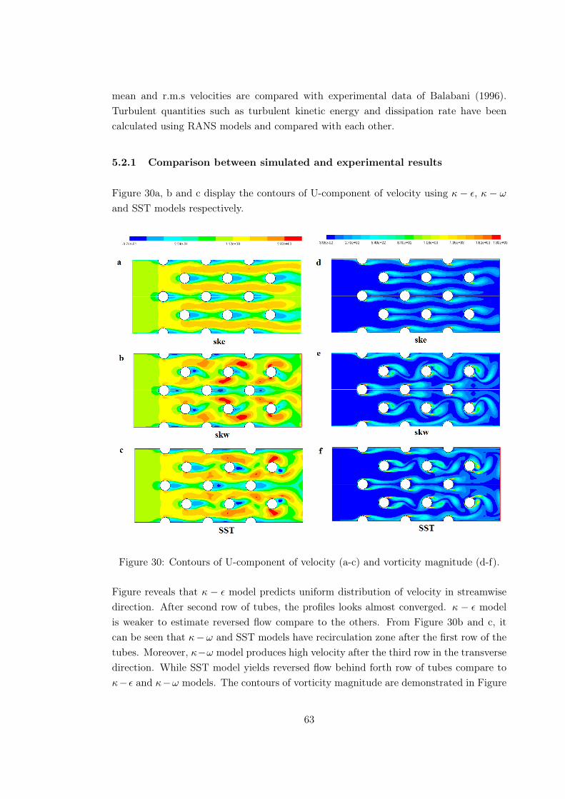
mean and r.m.s velocities are compared with experimental data of Balabani (1996).Turbulent quantities such as turbulent kinetic energy and dissipation rate have beencalculated using RANS models and compared with each other.
5.2.1 Comparison between simulated and experimental results
Figure 30a, b and c display the contours of U-component of velocity using κ− ε, κ− ωand SST models respectively.
Figure 30: Contours of U-component of velocity (a-c) and vorticity magnitude (d-f).
Figure reveals that κ − ε model predicts uniform distribution of velocity in streamwisedirection. After second row of tubes, the profiles looks almost converged. κ − ε modelis weaker to estimate reversed flow compare to the others. From Figure 30b and c, itcan be seen that κ−ω and SST models have recirculation zone after the first row of thetubes. Moreover, κ−ω model produces high velocity after the third row in the transversedirection. While SST model yields reversed flow behind forth row of tubes compare toκ− ε and κ−ω models. The contours of vorticity magnitude are demonstrated in Figure
63

30d, e and f with κ − ε, κ − ω and SST models. From Figure 30d, it is fact that κ − εis poor to predict vorticity behind tubes. It can be discerned that in κ − ω and SSTmodels, flow perturbations due to the unsteady nature of the vortex shedding becomemore prominent for the downstream rows of the tube bundle. In addition, it can be seenthat the maximum vortex formation length is behind the first row for κ − ω and SSTmodels. The one behind the second row is clearly shorter, which is consistent with therecirculation zone.
Figure 31: Contours of velocity vectors of SST model.
Figure 31 presents the velocity vector profile using SST model. It is interesting to notethat the pair of narrow recirculation zones in the wake is generating a strong and wideback-flow. From figure, it is clear that the SST model is able to predict the inverse flow.
During the initial part of calculations, the fluctuation are very large. when the timegoes, the flow becomes nearly stable with small fluctuation. By considering this fact inorder to get better agreement with the experiment results, for all the simulations, wehave taken time averaged value for several seconds. To check the ability of the mentionedturbulence models, eight different x/d locations like 0.85, 1.25, 2.95, 3.35, 5.05, 5.45, 7.15and 7.55, have been chosen. Paul et al. classified this flow into a developing region atx/d = 0.85 to 3.35 and a developed (spatially periodic) region at x/d ≥ 5.05 [29].
Figure 32 compares predicted and experimental values of the streamwise mean velocityat selected axial locations. Figure reveals that all the turbulence models produce thecorrect trends of the streamwise mean velocity profiles at all x/d locations. κ− ε, κ− ωand SST models appear to be in better agreement with the experimental data in theflow developing region at x/d = 0.85 to 3.35. while the SST model perform good in thespatially periodic region at x/d = 5.05 and 5.45 compared to the κ− ε and κ−ω models.From figure, it can be seen that all models give some variation with the experimental atx/d = 7.15 and 7.55
64

Figure 32: Comparison between profiles of predicted streamwise mean velocity withexperimental values at selected axial locations.
65

Figure 33: Comparison between profiles of predicted transverse mean velocity with ex-perimental values at selected axial locations.
66

Figure 33 shows the comparison between predicted transverse mean velocity with exper-imental values at some x/d locations. κ − ε, κ − ω and SST models are demonstratedgood results for x/d = 0.85 and 1.25. It is clear from these figures that the κ − ω
model significantly over predicts the experimental values of transverse mean velocity atx/d = 2.95 to 7.55. All the models overestimate in the developed region at x/d = 5.05.While the κ− ε model gives good agreement compared to the κ− ω and SST models atx/d = 5.45 to 7.55.
In Figure 34 the velocity fluctuations of streamwise are compared to the experimentalat selected axial locations. The κ−ω and SST models yield better correspondence withthe experimental at x/d = 0.85 and 1.25 than the κ − ε model. Not only are the fluc-tuation levels closer to the experimental, but the trends of the profiles are also in betteragreement. This indicates that the present simulation correctly predicts the productionof turbulence and any transitional phenomena that may appear in the boundary layer.The κ− ω predicts good correspondence with the experimental for the velocity fluctua-tion of streamwise at y = 0. All three turbulence models are failed to give results of thefluctuation velocity for 2.95 and 3.35 axial locations.
Figure 34: Comparison between profiles of predicted streamwise fluctuations of the ve-locity component with experimental values at selected axial locations.
67
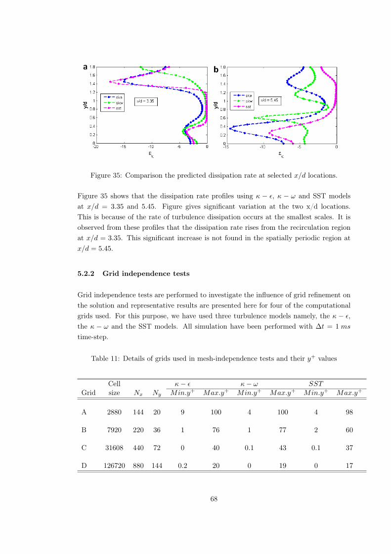
Figure 35: Comparison the predicted dissipation rate at selected x/d locations.
Figure 35 shows that the dissipation rate profiles using κ − ε, κ − ω and SST modelsat x/d = 3.35 and 5.45. Figure gives significant variation at the two x/d locations.This is because of the rate of turbulence dissipation occurs at the smallest scales. It isobserved from these profiles that the dissipation rate rises from the recirculation regionat x/d = 3.35. This significant increase is not found in the spatially periodic region atx/d = 5.45.
5.2.2 Grid independence tests
Grid independence tests are performed to investigate the influence of grid refinement onthe solution and representative results are presented here for four of the computationalgrids used. For this purpose, we have used three turbulence models namely, the κ − ε,the κ − ω and the SST models. All simulation have been performed with ∆t = 1 mstime-step.
Table 11: Details of grids used in mesh-independence tests and their y+ values
Cell κ− ε κ− ω SSTGrid size Nx Ny Min.y+ Max.y+ Min.y+ Max.y+ Min.y+ Max.y+
A 2880 144 20 9 100 4 100 4 98
B 7920 220 36 1 76 1 77 2 60
C 31608 440 72 0 40 0.1 43 0.1 37
D 126720 880 144 0.2 20 0 19 0 17
68

Table 11 provides some details of the grids, including the total number of nodes, thenumbers of nodes in the x- and y-directions, and minimum and maximum valves of they+ for each model. Here, Nx and Ny display the number of nodes in the x- and y-directions respectively. It should be noted that Grid A is very coarse and has large max.y+ values for all three turbulence models.
Figure 36: Contours of turbulent kinetic energy with (a) Grid A, (b) Grid B, (c) GridC, and (d) Grid D using SST model.
Figure 37: Contours of U-component of velocity with (a) Grid A, (b) Grid B, (c) GridC, and (d) Grid D using SST model.
69

Figure 36 demonstrates contours of turbulent kinetic energy (TKE) produce by differentgrids using SST model. It is clear that the spatially periodic region is much sensitive withgrid refinement compared to the developing region in tube bundles. In developed region,the Grid A gives low turbulent kinetic energy than other grids while Grid D predictshigh turbulent kinetic energy. Contours of U-component of velocity with different gridare shown in Figure 37. From figure, it can clearly observed that there is a variationin the U-component of velocity profiles when we refine the grid from Grid B to GridD. It can be seen that Grid A and B yield high transverse velocity in developed regioncompared to Grid C and D. Moreover, very fine Grid D produces different profile thanother grids.
For grid sensitivity, two samples of the results in the developing region, x/d = 1.25 andthe spatially periodic region, x/d = 5.45 have been chosen. Following Figure 38 predictsthe profiles of grid-independence test of streamwise mean velocity at x/d = 1.25 and5.45 using κ − ε, κ − ω and SST models. Figure 38a and b show that there are no anysignificant changes when refinement in the grids from Grid A to Grid D in the κ−εmodel.Where Figure 38c to f yield results of κ− ω and SST models, which are quite sensitiveto grid resolution changes. In the developing region, x/d = 1.25 the κ − ω and SSTmodels give not much variation compared to the spatially periodic region, x/d = 5.45.In both models Grid D produce significant change than other grids in the streamwisemean velocity at x/d = 5.45. Sample profiles of grid-independence test of transversemean velocity at x/d = 1.25 and 5.45 are shown in Figure 39. It can be seen that theκ − ε has no grid sensitivity in the V-component of velocity for both regions. Figure39c and d demonstrate the results of κ− ω model. It is observed that there tends to begreater changes with grid resolution in the κ−ω results at x/d = 5.45 to the 1.25. GridsA and C are overestimate the transverse mean velocity at x/d = 5.45 compared to theexperimental valves. Also in Figure 39e and f, there are more variation in the SST modelresults at x/d = 5.45 to the 1.25. In SST model Grids A and B give greater changesthan Grids C and D in the spatially periodic region. The results for the κ− ω and SSTmodels show somewhat higher differences from Grid A to D, especially at x/d = 5.45.
Figure 40 reveals the profiles of grid-independence test of turbulent kinetic energy atselected axial locations. It can be observed that all three model are affected by gridin turbulent kinetic energy. In addition, it is also clear that there tends have greaterchanges with grid refinement in the κ− ω and SST models results at x/d = 5.45 to the1.25. In order to check, Grids A and D predict high turbulent kinetic energy comparedto other grids in the κ − ω. While Grid D gives more turbulent kinetic energy thanremain grids in the SST model.
70

Figure 38: Profiles of grid-independence test of streamwise mean velocity at x/d = 1.25and 5.45.
71

Figure 39: Profiles of grid-independence test of transverse mean velocity at x/d = 1.25and 5.45.
72

Figure 40: Profiles of grid-independence test of turbulent kinetic energy at x/d = 1.25and 5.45.
5.2.3 Time-step sensitivity study
In order to check the effect of time-step, ∆t, on the results, three different time-stepas 10 ms, 1 ms and 0.25 ms have been chosen. In this section, all the simulations havebeen performed with Grid C. We have calculated the streamwise and transverse meanvelocities using the κ−ε, κ−ω and SST models. Here we have chosen two samples of theresults in the developing region, x/d = 3.35 and the spatially periodic region, x/d = 5.45.
73

In addition, for better convergence we have fixed 20 iterations per time-step. For goodagreement with experimental values, time averaged value have been calculated for severaltime.
Following Figure 41 reveals that streamwise mean velocity with experimental using dif-ferent time-steps. The results obtained at three different time-steps for exactly the sameoperating conditions and apparatus. Figure 41a and b show that the κ− ε model is notsensitive to time-step changes beyond a certain time-step in both, the developing andthe spatially periodic regions. This trend is similar for the results for transverse meanvelocity shown in Figure 42a and b.
Figure 41: Time-step effect on streamwise mean velocity at x/d = 3.35 and 5.45.
74

In Figure 41c and d the U-component of velocity compared to the experimental valuewhich is obtained from the κ − ω model. There are quite variation in the results withtime-step changes at x/d = 3.35 and x/d = 5.45. It is fact that the ∆t = 0.25 ms givesbetter correspondence with the experimental than other two time-steps.
Figure 42: Time-step effect on transverse mean velocity at x/d = 3.35 and 5.45.
From Figure 42c and d, it is clear that the κ− ω predicts the higher value of transversemean velocity with ∆t = 1 ms in both regions. Figure 41e and f yield the profile ofstreamwise mean velocity with experimental for SST model using various time-steps.At x/d = 3.35 position, the SST gives satisfactory agreement with the experimentalbut there are some points where the streamwise mean velocity level remains high when
75

compared to the experimental in the recirculation zones. Figure reveals that the SSTmodel produce the correct trends of the streamwise mean velocity profiles at x/d =3.35 while in the spatially periodic region, x/d = 5.45, there is more variation in therecirculation zones with time-step changes. On the other hand, Figure 42e and f showthat the SST model is quite sensitive to time-step changes in the transverse mean velocityat x/d = 3.35 and x/d = 5.45. From figure, the ∆t = 0.25 ms results are near toexperimental than other two time-steps. The mean velocity profiles seem to be in goodagreement near the recirculation regions when compared to the ∆t = 0.25 ms time step.
5.2.4 Sensitivity of the model constants C1ε and C2ε in κ− ε model
In the RANS based κ − ε model as it has been discussed in Chapter 3, there are fourmodel constants in the equations of κ and ε. The value of model constants are given inEq. (65) which are fixed by Launder and Spalding 1974 [1]. These values are based onextensive examination of free turbulent flows, but they can also be used for wall flows. Asensitivity study has shown that the calculations are most sensitive to the values of C1ε
and C2ε. Literature says that if changes in C1ε or C2ε up to 5% then the results affectedup to 20% [30].
In order to check this sensitivity, we have chosen C1ε and C2ε model constants. Due tothis, we have taken ±5% change in the original values of model constants. By consideringthese changed values, the streamwise and transverse mean velocities, turbulent kineticenergy and dissipation rate have been calculated.
Following Figure 43 represents the comparison between predicted streamwise and trans-verse mean velocities with experimental values at selected axial locations. Streamwisemean velocity profiles with ±5% change in C1ε are given in Figure 43a to d. It can beobserved that there is no any significant change at x/d = 1.25 when changed in C1ε.Figure reveals that the trends of the profiles have good agreement with experimental.However, there are some variation in the results of the spatially periodic region comparedto the developing region when changes in model constant values. Figure 43e to h displaythe transverse mean velocities with experimental values at selected axial locations. It isinteresting to see that there is no any remarkable change when we decrease 5% value ofC1ε. While increment in the value of C1ε is sensitive for y-component of velocity. Forx/d = 3.35, 5.45 and 7.55, transverse mean velocity have been affected with increasedvalue of C1ε. In addition, to ensure the effect of changes in the C1ε for turbulent kineticenergy, we have chosen four axial locations.
76

Figure 43: Comparison between profiles of predicted streamwise (a-d) and transverse(e-f) mean velocities with experimental values at selected axial locations.
77

Figure 44: Comparison the predicted turbulent kinetic energy at selected x/d locations.
Figure 45: Comparison the predicted dissipation rate at selected x/d locations.
78
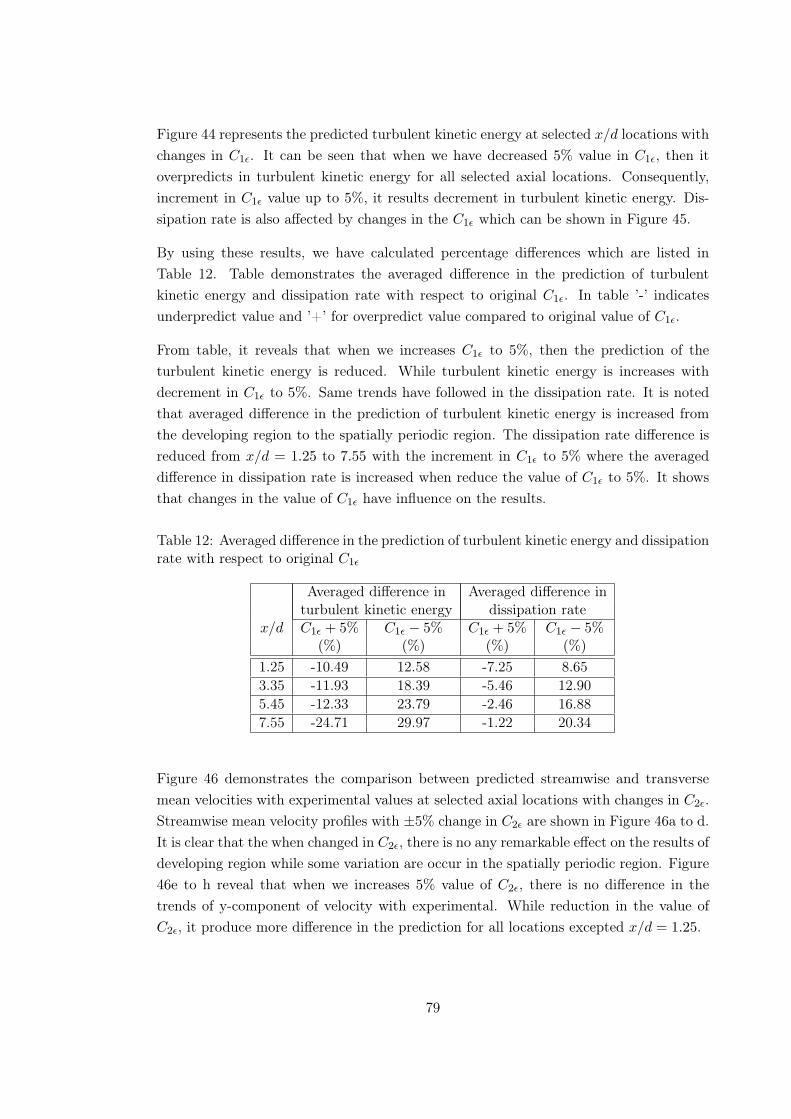
Figure 44 represents the predicted turbulent kinetic energy at selected x/d locations withchanges in C1ε. It can be seen that when we have decreased 5% value in C1ε, then itoverpredicts in turbulent kinetic energy for all selected axial locations. Consequently,increment in C1ε value up to 5%, it results decrement in turbulent kinetic energy. Dis-sipation rate is also affected by changes in the C1ε which can be shown in Figure 45.
By using these results, we have calculated percentage differences which are listed inTable 12. Table demonstrates the averaged difference in the prediction of turbulentkinetic energy and dissipation rate with respect to original C1ε. In table ’-’ indicatesunderpredict value and ’+’ for overpredict value compared to original value of C1ε.
From table, it reveals that when we increases C1ε to 5%, then the prediction of theturbulent kinetic energy is reduced. While turbulent kinetic energy is increases withdecrement in C1ε to 5%. Same trends have followed in the dissipation rate. It is notedthat averaged difference in the prediction of turbulent kinetic energy is increased fromthe developing region to the spatially periodic region. The dissipation rate difference isreduced from x/d = 1.25 to 7.55 with the increment in C1ε to 5% where the averageddifference in dissipation rate is increased when reduce the value of C1ε to 5%. It showsthat changes in the value of C1ε have influence on the results.
Table 12: Averaged difference in the prediction of turbulent kinetic energy and dissipationrate with respect to original C1ε
Averaged difference in Averaged difference inturbulent kinetic energy dissipation rate
x/d C1ε + 5% C1ε − 5% C1ε + 5% C1ε − 5%(%) (%) (%) (%)
1.25 -10.49 12.58 -7.25 8.653.35 -11.93 18.39 -5.46 12.905.45 -12.33 23.79 -2.46 16.887.55 -24.71 29.97 -1.22 20.34
Figure 46 demonstrates the comparison between predicted streamwise and transversemean velocities with experimental values at selected axial locations with changes in C2ε.Streamwise mean velocity profiles with ±5% change in C2ε are shown in Figure 46a to d.It is clear that the when changed in C2ε, there is no any remarkable effect on the results ofdeveloping region while some variation are occur in the spatially periodic region. Figure46e to h reveal that when we increases 5% value of C2ε, there is no difference in thetrends of y-component of velocity with experimental. While reduction in the value ofC2ε, it produce more difference in the prediction for all locations excepted x/d = 1.25.
79

Figure 46: Comparison between profiles of predicted streamwise (a-d) and transverse(e-f) mean velocity with experimental values at selected axial locations.
80

Figure 47: Comparison the predicted turbulent kinetic energy at selected x/d locations.
Figure 48: Comparison the predicted dissipation rate at selected x/d locations.
81

The sensitivity of C2ε on the turbulent kinetic energy which is given in Figure 47. It canbe observed that when we decreases 5% value in C2ε, then it predicts lower value of tur-bulent kinetic energy compared to original value at selected axial locations. Furthermore,increment in C2ε up to 5%, it results higher value than original. Figure 48 describes thedissipation rate at selected x/d locations. There is some variation in predicted value ofthe dissipation rate when changes in C2ε.
Table 13 demonstrates the averaged difference in the prediction of turbulent kineticenergy and dissipation rate with respect to original C2ε. In table ’-’ indicates underpredictvalue and ’+’ for overpredict value compared to original value of C2ε.
Table shows that the prediction of the turbulent kinetic energy is increased, when weincreases C2ε to 5%. While turbulent kinetic energy is reduced with decrement in C2ε to5%. Same behavior have followed by the averaged difference of dissipation rate. Fromthis discussion, it can be observed that value of C2ε have considerable impact on theresults.
Table 13: Averaged difference in the prediction of turbulent kinetic energy and dissipationrate with respect to original C2ε
Averaged difference in Averaged difference inturbulent kinetic energy dissipation rate
x/d C2ε + 5% C2ε − 5% C2ε + 5% C2ε − 5%(%) (%) (%) (%)
1.25 4.11 -3.97 1.02 -0.423.35 12.50 -10.03 6.62 -4.485.45 17.55 -23.23 10.13 -23.527.55 24.90 -0.11 15.14 28.35
82

6 Conclusions
In the present work, the flow past a circular cylinder at sub-critical Reynolds numbersof ReD = 1000 and 3900 were simulated by using the RANS and the LES approaches.Critical flow parameters, which are time-averaged drag coefficient, Strouhal number, flowseparation angle, pressure distribution on the surface of cylinder and vortex sheddingin the wake region of the cylinder have been predicted with each turbulence modeland some of them calculated values are compared with experimental. Moreover, gridrefinement and time-step effect study have been analyzed with ReD = 1000. The resultsof the present numerical investigation of flow past a circular cylinder demonstrate thefollowing conclusions.
• The study with ReD = 1000, among the κ − ε, SST and LES models, the SSTmodel yielded the ability to predict the mean value of the drag coefficient similarto experimental data. The LES model produced an accurate agreement with theexperimental data for the Strouhal number while the RANS models failed to pre-dict. The κ−ε and SST models indicate a much delayed flow separation for ReD =1000 when LES computed separation point close to experimental value comparedto the RANS. The κ− ε and the SST models overestimated the pressure gradienton windward and leeward side of the cylinder while the LES model has been closelyrelated to the experimental value. The LES model provides more realistic picturesfor the vortex shedding flow in the transitional flow regime. But the κ − ε andthe SST models are not able to predict vortex shedding in the wake region of thecylinder.
• The LES model have good predicted the drag coefficient, Strouhal number andseparation point of the flow and closed to the experimental value for ReD = 3900.While the κ− ε and SST models produced good agreement with experimental forseparation angle but they have underpredicted the drag coefficient compared to theexperimental value for Reynolds number of 3900. The pressure distribution aroundthe cylinder surface from the κ−ε and SST models agreed well with measured datain the windward region excepted the stagnation point and flow separation regionbut no unsteadiness of flow have been observed in the wake region. The LES modelhas better agreement with the experimental for the pressure distribution aroundthe cylinder surface for ReD = 3900. In the LES computations, the unsteady scalesof the flow and vortex structure has been well predicted.
• The effect of grid resolution was tested with the κ−ε, SST and LES models. It hasbeen observed that the SST model predicted drag coefficient close to experimentalresults at ReD = 1000 with all selected grids compared to the κ − ε model. TheLES model have been illustrated close agreement with experimental values for drag
83

coefficient and flow separation point using grid resolution. Hence, the LES modelhas a major influence on the grid size of the computational domain to predictcritical flow parameters. The calculation of Strouhal number from the LES modelhave been expressed that it is grid independence. Moreover, in the prediction ofvortex shedding, three-dimensional vortical structures behind the cylinder havebeen lost in the coarse grid while very fine grid have good strength to estimate it.So, it reveals that finer grid is necessary to capture details information for vortexshedding by using LES model.
• In the study of time-step effect, it can be concluded that the time step has a littleinfluence in the prediction of the drag coefficient and vortex shedding while it isnot sensitive for the Strouhal number in LES model with Reynolds number of 1000.
In the present study, time dependent calculations of the subcritical cross flow througha staggered tube bundle have been performed in two dimension with the κ − ε, κ − ωand SST models. The streamwise and transverse, mean and r.m.s velocities have beencalculated with each turbulence model and compared with experimental data. Turbulentquantities such as turbulent kinetic energy and dissipation rate were presented by usingthe κ − ε, κ − ω and SST models. In addition, grid independence tests and time-stepsensitivity study have been done with all three models. Study concerning the sensitivityof model constants C1ε and C2ε have been conducted. The results of the present studiesof turbulent flow in a staggered tube bundle yield the following conclusions.
• Comparisons between the numerical and experimental values demonstrate thatthe streamwise mean velocity profiles were reasonably well predicted by all theturbulence models. It is observed that the κ − ε and SST models produced goodagreement with experimental for the transverse mean velocity compared to theκ − ω model. The prediction of the velocity fluctuation from each models havesignificant variation compared to the experimental value. It have been illustratedthat the dissipation rate produced from each model have reached maxima in therecirculation region while much smaller in magnitude outside the recirculation re-gion.
• By using four different grids, simulations have been carried out with the κ−ε, κ−ωand SST models. The κ−ε showed less sensitivity to changes in the grid resolutionfor both streamwise and transverse mean velocities. Where the κ − ω and SSTmodels have been affected by the grid refinement in the spatially periodic region.It was pronounced that the turbulent kinetic energy have substantial differencewith grid changes in the spatially periodic region compared to developing regionfor all models. Hence, it is clear that grid refinement is required to achieve betteragreement with experimental value.
84

• The study concerning time-step effect on the results have been done using threedifferent time-step sizes. It is noted that results produced from κ− ε model, haveno any variation using different time-step. Both streamwise and transverse meanvelocities have considerable effect with time-step changes for κ−ω and SST modelsand fine time-step has good correspondence with experimental.
• Model constants sensitivity study have been conducted by adopting κ − ε modelwith changes the value ±5%. It was observed that reduction in the value of C1ε,no more significant variation has been noted in streamwise and transverse meanvelocities compared to original value of model constant. But increment of C1ε to5% has produced remarkable change in the transverse mean velocity. Moreover, theaveraged difference compared to original model constant value for the predictionof turbulent kinetic energy and dissipation rate are inversely proportional to theC1ε. It was noted that increment of C2ε to 5% displayed significant change in theprediction of transverse mean velocity compared to original value of model constantwhile decrement in the value of C2ε produced no any variation. Study showsthat there is a proportional relation between the averaged difference compared tooriginal model constant value of turbulent kinetic energy and C2ε. This same trendhave followed by dissipation rate for all selected locations but it has failed to obeythis trend at x/d = 7.55 when reduced the value of C2ε to 5%.
85

References
[1] Versteeg, H. K., and Malalasekera, W., (2007). An introduction to computational fluiddynamics , second edition. Prentice Hall, England.
[2] White, F. M., (1974). Viscous fluid flow, First edition. Printed in USA.
[3] Blazek, J., (2001). Computational fluid dynamics: principles and applications, First edition.Printed in Netherlands.
[4] Wilcox, D. C., (2004). Turbulence modeling for CFD, Second edition. Printed in the Cali-fornia.
[5] McDonough, J. M., (2004). Introductory lectures on turbulence physics, mathematics andmodeling, Departments of Mechanical Engineering and Mathematics, University of Ken-tucky
[6] Pepper, D. W., and Carrington, David., (2009).Modeling indoor air pollution , First edition.Printed in Singapore.
[7] Zdravkovich, M. M., (1997). Flow around circular cylinders Vol 1: fundamentals , Firstedition. Printed in Oxford University Press, New York.
[8] ANSYS FLUENT 12.1 Theory Guide, (2010).
[9] Bakker, A.,Turbulence models, Lecture material, Applied Computational Fluid Dynamics.
[10] Jones, D. A., and Clarke, D. B., (2008). Simulation of flow past a sphere using the Fluentcode , Published by Maritime Platforms Division, DSTO Defence Science and TechnologyOrganisation, Australia.
[11] Bloor, M. S., The transition to turbulence in the wake of a circular cylinder, Journal ofFluid Mechanics, 1964, Vol.19, p. 290-304.
[12] Tutar, M., and HoldØ, A. E., (2001). Computational modelling of flow around a circularcylinder in sub-critical flow regime with various turbulence models, Journal of NumericalMethods in Fluids, Vol.35, p. 763-784.
[13] Bouris, D., and Bergeles, G., (1998). Two dimensional time dependent simulation of thesubcritical flow in a staggered tube bundle using a subgrid scale model, Journal of Heat andFluid Flow, Vol.20, p. 105-114.
[14] Tannehill, J. C., Anderson, D. A., Richard, H., (1997). Computational fluid mechanics andheat transfer, Second addition, Taylor and Francis, London.
[15] Anderson, D. John,. (1995). Computational fluid dynamics , First edition. Printed inSingapore.
[16] Launder, B. E., and Spalding, D. B., (1972). Mathematical models of turbulence , Depart-ments of Mechanical Engineering, Imperial College of Science and Technology, London,England
[17] Biswas, G., and Eswaran, V., (2002). Turbulent flows fundamentals, experiments andmodeling, First edition. Printed in India.
[18] Zevenhoven, Ron,. (2009). Introduction to computational fluid dynamics, Lecture notes.Heat Engineering Laboratory, Ĺbo Akademi University, Finland.
86

[19] Ferrey, P., and Aupoix, B., (2006). Behaviour of turbulence models near a turbulent/non-turbulent interface revisited, Journal of Heat and Fluid Flow, Vol.27, p. 831-837.
[20] Jurij, S., (2007). Turbulence models in CFD, Lecture note, University of Ljubljana.
[21] Bell, B., (2003). Turbulent flow cases, Fluent Inc.
[22] Rahman, M., Karim, M., and Alim, A., (2007). Numerical invertigation of unsteady flowpast a circular cylinder using 2-D finite volume method, Journal of Naval Architecture andMarine Engineering, Vol.4, p. 27-42.
[23] Ünal, U. O., and Gören, Ö., (2005). Vortex shedding from a circular cylinder at highReynolds number, Istanbul Technical University, Department of Naval Architecture, Istan-bul, Turkey.
[24] Balabani, S., and Yianneskis, M., (1996). An experimental study of the mean flow andturbulence structure of cross-flow over tube bundles., Proc. Instn. Mech. Engrs., Vol.210, p.317-331.
[25] Hill, R., Shim, K., Lewis, R., (1986). Sources of excitation in tube banks due to vortexshedding., Proc. Instn. Mech. Engnrs., Vol.200, p. 293-301.
[26] Zdravistch, F., Fletcher, C., and Behnia, M., (1995). Numerical laminar and turbulentfluid-flow and heat transfer predictions in tube banks., Int. J. Num. Methods for Heat andFluid Flow, Vol.5, p. 717-733.
[27] Balabani, S., Bergeles, G., Burry, D., Yianneskis, M., (1994). Velocity characteristics ofthe cross-flow over tube bundles., In: International Proceedings of the 7th InternationalSymposium on Application of Laser Anemometry to Fluid Mechanics, Lisbon, vol. 2, p.39.3.1–39.3.8.
[28] Bouris, D., Bergeles, G., (1999). Two dimensional time dependent simulation of the sub-critical flow in a staggered tube bundle using a subgrid scale model. Int. J. Heat Fluid Flow,Vol.20, p. 105–114.
[29] Paul, S.S., Tachie, M.F., and Ormiston, S.J., (2007). Experimental study of turbulent cross-flow in a staggered tube bundle using particle image velocimetry., Int. J. Heat Fluid Flow,Vol.28, p.441–453.
[30] Rodi, W., (1980). Turbulence models and their application in hydraulics-A state of the Art.,IAHR, Delf, The Netherlands.
[31] Dyke, M. V., (1982). Album of fluid Motion, Parabolic Press, UK.
87