numerical investigation of drag reduction using ... · numerical investigation of drag reduction...

Journal of Engineering Technology Volume 3, Issue 2, July, 2015, Pages. 158-173

Numerical Investigation of Drag Reduction Using

Electromagnetic

Reza Soleimanpour1* and Kazem Kalantari

2

1,2- MSc of Mechanical Engineering, Kish International Branch, Islamic Azad Univesity,

Kish Island, Iran

Abstract. In recent years, numerous experimental and numerical methods

have been used for drag reduction. One of the most effective methods to

reduce drag and turbulent boundary layer control is applying the

electromagnetic. The aim of this project is to reduce drag and increase lift by

using the electromagnetic effect. Various studies conducted by researchers in

the field using electromagnetic drag reduction are investigated. In addition,

the use of electromagnetic modes to reduce the drag of a flat plate using

numerical methods and software CFX and comsol simulated. Research

carried out by different people, as well as simulations show that the drag

reduction of up to 50 percent through the use of electromagnetic forces to the

fluid is possible.

Keywords: Hydrofoil, flow separation, dragforce, electromagnetic, CFX.

1 Introduction

One of the effective methods to reduce drag and turbulence boundary control

is using electromagnetic, or properly is forces caused by the

electromagnetic. It should be noted that if a fluid such as water that has

electrical conductivity, passes from the electromagnetic field, forces that is

knownLorentz force applied to it, this force is applied in different ways in

order to reduce drag.In most studies, direction ofLorentz force was in fluids

direction that has actually acted as an accelerator in the fluid direction and as

an electromagnetic pump [1]. Gailitis and Lielausis [quotedfrom reference

[6] was the first group who used Lorentz force to control fluid. In

www.joetsite.com


theiranalysis, they appliedLorentzforce to the fluid laminar boundarylayer in

fluid direction in order to create a thrust force and also prevent

fromtransferring of laminar boundary layer to turbulent layer and increasing

of thethickness of boundary layer [quoted from reference 2]. Shtern and

Nosenchuckshowed that the Blasius profile of boundary layer when the

Lorentzforce is appliedit become more stable.

Nosenchuck and his team [quoted from [7] studied viscous drag reduction on

Boundarylayer, usingLorentzforce, In their experiments , Lawrence force is

in perpendicular direction to the wall and perpendicular to the flow direction.

Their aim has been drag reductionbycontrolling turbulenceBoundary layer.

The results were not showing drag reduction and could not achieve the

resultsby applying Lorentz forcein drag reduction.Bandyopadhyayand

Castanoplaced arrangement of the electrodes and magnets as Henoch, but

considereddirection of flow perpendicular to the Lawrence force. They

connected electrodes to an alternating current that causes the Lawrence force

applied to the fluid, shift with flow frequency.

In fact, an oscillatory force is applied to the fluid and as the same as the

surface of the object that fluid is moving has a swinging motion. Simulations

show 30 percent of drag reduction that of course depends on the current

frequency, or in other words the Lorentz force. The cause of drag reductionis

turbulence reduction ofBoundary layer through combining

ofvortexresonance in Boundary layer and also applied Lorentzforce, but in

laboratory method they could not reach the amount of drag reduction

obtained in the simulation. In the laboratory method, they obtained only 3%

of drag reduction [quoted from reference 9].

2 Statement of the problem

Thisstudy has been evaluatedairfoil NACA 0012 geometry. In order to draw

the desired geometry in Gambit software, the following equation was used.

First, using this relationship and ratio x / c between 0 to 1 and chord one,

about 100 data obtained with different coordinates , saved in TEXT format ,

called in the Gambit software and then is drawing. In this software,

afterdrawing of lines, meshing(channeling) of computing field is discussed.

The final form of the descriptive geometry is in the form of (1). The

boundary conditions used for the computational domain of the boundary

condition is pressure far field.

www.joetsite.com


2 3

4

0.298222773 0.127125232

.594689181 0.357906 0.291984971

0.105174696

x x

c c

x xy c o

c c

x

c

Figure. 1. Geometry of a NACA 0012 with chord equal 1

After drawing of geometry and meshing in related geometry Gambit

software, it is called in CFX software. To simulate, the initial conditions is

required, to do so, the data in the paper [41] was applied as table (1).

Table.1. the initial conditions used in the simulation

entrance

speed(m/s) 05

density(kg/m3) 352/1

temperature(oC) 35

viscosity(kg/ms) 71218/1

Mach 10/5

3 Independence of the results from meshing

In each simulation, in order to ensure computational domain and

independence of meshing solutions must ensure proper meshing. In this

regard, the airfoil has been evaluated using different meshing and comparing

www.joetsite.com


the results to predict the lift coefficient on the angle of attack of 2 degree,

and the results for (2) is given. As seen, the results for a lattice of up to

70,000 predict almost equal results, so the same number of lattice will be

used to continue the work.

Figure. 2. Study of meshing and the independence solution results from the number of

lattice

4 Authentication method

Figure (3) shows the lift coefficient at different angles of attack for the

boundary conditions mentioned in the table (1) and its comparison with the

data in the paper [41]. As you can see, the results of the simulation for angles

of attack higher than 6, gradually is increasing the error. The reason for this

difference may be due to segregation, which occurring during the flow, the

model could not predict it. The process for different turbulence models and

meshing more than 70000 has been investigated and still has erroneous

results. Hence it is evident that CFX software for this case study does not

predict a good outcome. So considering the purpose of this project which is

the use of electromagnetic force, and taking into account the capability of

COMSOL software, as described here the COMSOL software is used.

www.joetsite.com


Figure. 3. Comparing the results of CFX software and experimental data

5 Computational domain

In order to predict the flow behavior in COMSOL software, the intended

computational domain was in the form of figure (4) respectively. It is seen

that the computing field about 200 times the chord that is equal 1/8 (Figure

(5)) is drawn in the back and about 100 times in the front of airfoil. The

implied Boundary conditions are based on the figure. The initial conditions

used based on the table (2) with the exception that the Reynolds number of

the basic chord is 6 × 106.

Figure. 4. computational domain for simulation in COMSOL software

www.joetsite.com


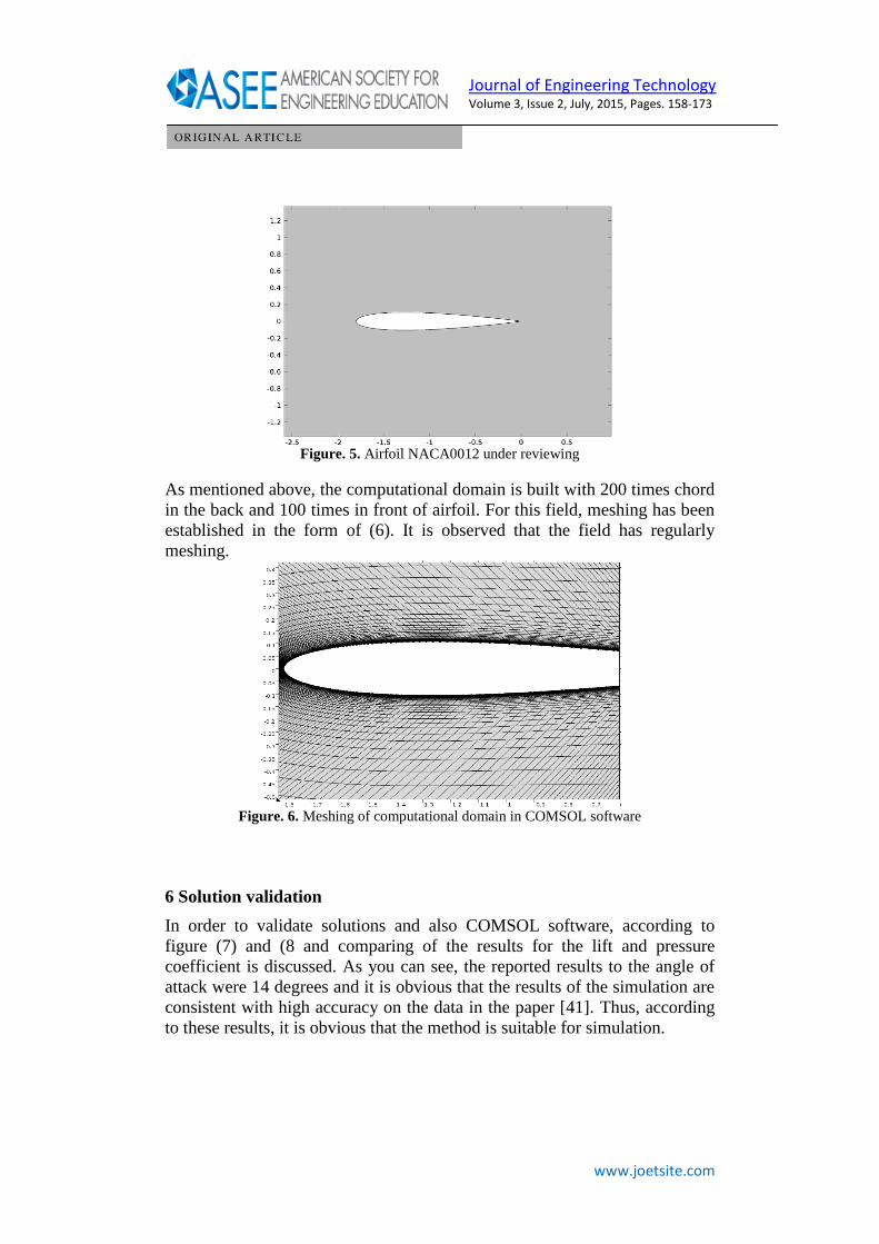
Figure. 5. Airfoil NACA0012 under reviewing

As mentioned above, the computational domain is built with 200 times chord

in the back and 100 times in front of airfoil. For this field, meshing has been

established in the form of (6). It is observed that the field has regularly

meshing.

Figure. 6. Meshing of computational domain in COMSOL software

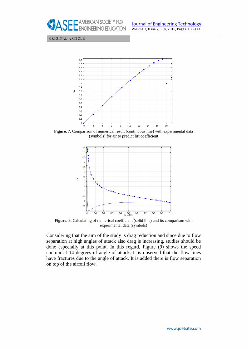
6 Solution validation

In order to validate solutions and also COMSOL software, according to

figure (7) and (8 and comparing of the results for the lift and pressure

coefficient is discussed. As you can see, the reported results to the angle of

attack were 14 degrees and it is obvious that the results of the simulation are

consistent with high accuracy on the data in the paper [41]. Thus, according

to these results, it is obvious that the method is suitable for simulation.

www.joetsite.com


Figure. 7. Comparison of numerical result (continuous line) with experimental data

(symbols) for air to predict lift coefficient

Figure. 8. Calculating of numerical coefficient (solid line) and its comparison with

experimental data (symbols)

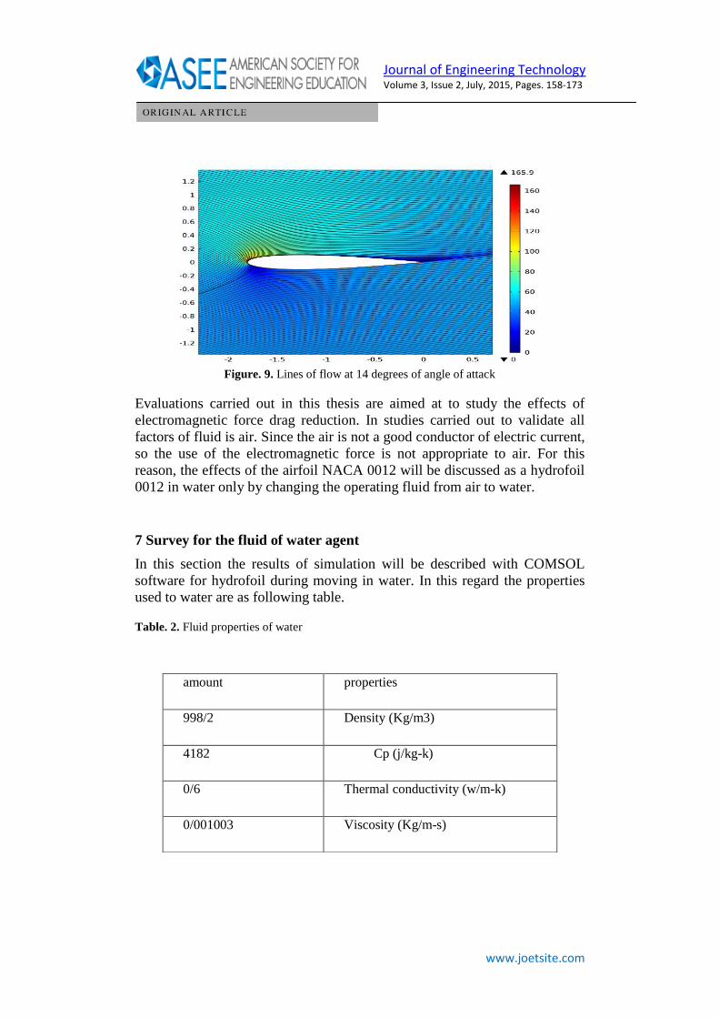
Considering that the aim of the study is drag reduction and since due to flow

separation at high angles of attack also drag is increasing, studies should be

done especially at this point. In this regard, Figure (9) shows the speed

contour at 14 degrees of angle of attack. It is observed that the flow lines

have fractures due to the angle of attack. It is added there is flow separation

on top of the airfoil flow.

www.joetsite.com


Figure. 9. Lines of flow at 14 degrees of angle of attack

Evaluations carried out in this thesis are aimed at to study the effects of

electromagnetic force drag reduction. In studies carried out to validate all

factors of fluid is air. Since the air is not a good conductor of electric current,

so the use of the electromagnetic force is not appropriate to air. For this

reason, the effects of the airfoil NACA 0012 will be discussed as a hydrofoil

0012 in water only by changing the operating fluid from air to water.

7 Survey for the fluid of water agent

In this section the results of simulation will be described with COMSOL

software for hydrofoil during moving in water. In this regard the properties

used to water are as following table.

Table. 2. Fluid properties of water

amount properties

998/2 Density (Kg/m3)

4182 Cp (j/kg-k)

0/6 Thermal conductivity (w/m-k)

0/001003 Viscosity (Kg/m-s)

www.joetsite.com


In addition, due to the physical properties of the water, during movement

with high-speed of solid object in the water ,are likely to cause cavitations

event , so to prevent from such occurrence and reliability of results, speed of

hydrofoil movement in the water, 2 meters per second would be The basis of

the work. The rest of the initial conditions are as table 1.

8 Analysis of the results

Figure (10) shows convergence diagrams for analysis of electromagnetic

force. As observed all the residuals is less than 3.10 and indicate

convergence of a problem solving with low remaining.

Figure. 10. Amount of computational errors at different angles of attack

157

×707813/3 Standard state enthalpy (j/kgmol)

31/21153 Standard state entropy (j/kgmol-k)

www.joetsite.com


Figure. 11. Hydrofoil lift coefficient distribution (solid line) for different angles of attack

Figure. 12. distribution hydrofoil drag coefficient for different angles of attack

Figure (13) shows the velocity distribution around hydrofoil and for angles

of attack, 13 and 14 degrees. As is visible at the end of hydrofoil for both

angles of attack the isolated form is applied, and it is an inevitable event in

the flying objects or submarine at high angles of attack. Separation of flow

causes drag increasing and each way to control this event would be an

effective method to reduce drag.

www.joetsite.com


Figure. 13. Velocity distribution contours for hydrofoil in angles of attack 13 and 14 degree

9 Electromagnetic force

This section examines the effects of electromagnetic force with the

conditions in the table (1) and a speed of 2 meters per second as well as the

flow of potential with 50,000 kilowatts. It is observed that there is no trace of

the existence of separation on the airfoil. Therefore, the use of

electromagnetic force can be used as a convenient way to control flow

separation.

www.joetsite.com


Figure. 14. velocity distribution contours for hydrofoil in 13 and 14 degree angles of attack

with the electromagnetic force

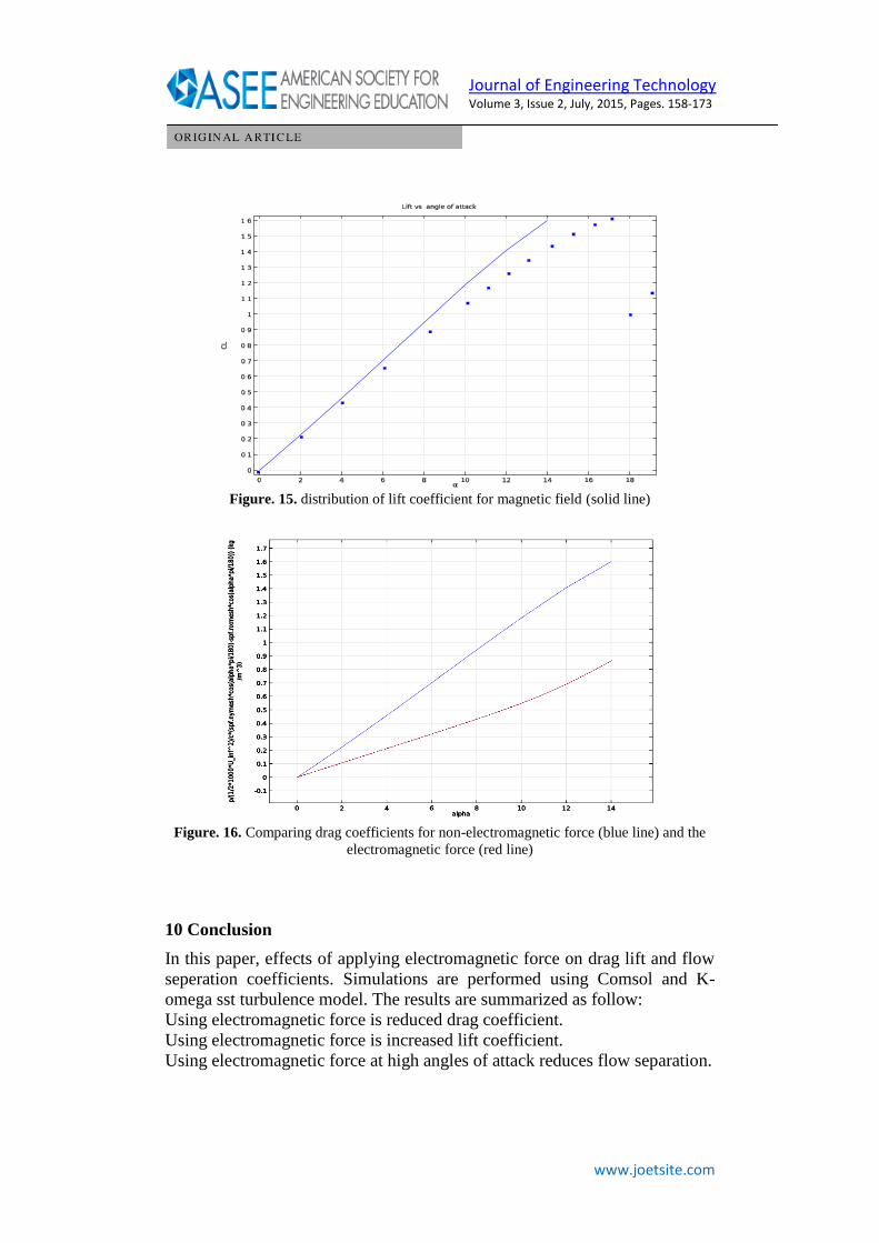
And also figures (15) and (16) show a comparison between lift and drag

coefficients for the non-use of the electromagnetic force and use of

electromagnetic force, respectively. It is observed that the application of an

electric field , increase the coefficient of lift (in comparison with figure (11))

and reduce the drag coefficient due to eliminate the effects of flow

separation.

www.joetsite.com


Figure. 15. distribution of lift coefficient for magnetic field (solid line)

Figure. 16. Comparing drag coefficients for non-electromagnetic force (blue line) and the

electromagnetic force (red line)

10 Conclusion

In this paper, effects of applying electromagnetic force on drag lift and flow

seperation coefficients. Simulations are performed using Comsol and K-

omega sst turbulence model. The results are summarized as follow:

Using electromagnetic force is reduced drag coefficient.

Using electromagnetic force is increased lift coefficient.

Using electromagnetic force at high angles of attack reduces flow separation.

www.joetsite.com


The limitations are listed as below:

Using COMSOL software require high RAM.

Computing time compared to the current two-dimensionality is high.

REFERENCES

1. Meng, J. C., Huyer, S. A., Castano, J. M., Thivierge, D. P., & Hendricks, P. J.

(1997). Experimental Study of the Spanwise Vortex Resonance Hypothesis for

Turbulent Drag Reduction over a Flat Plate in Salt Water: DTIC Document.

2. Berger, T.W., Kim, J., Lee, C., Lim, J.: Turbulent boundary layer control

utilizing the Lorentz force. Physics of Fluids, 12(3), 631-649 (2000).

doi:doi:http://dx.doi.org/ 10.1063/ 1.870270

3. Weier, T., Mutschke, G., Fey, U., Avilov, V., Gerbeth, G.: Electromagnetic

control of flow separation. Institute of Safety Research, 147-154 (1999).

4. Sura, D.: Electromagnetic Boundary Layer Control. MIT Sea Grant College

Program, Massachusetts Institute of Technology, (2003)

5. Ho. Joung et al., Response of spatially-developing turbulent boundary layer to

spanwise oscillating electromagnetic force, International Symposium on

Seawater Drag Reduction (2005).

6. Bushnell, D.M., Hefner, J.M.: Viscous drag reduction in boundary layers.

American Institute of Aeronautics and Astronautics, Washington, DC (1990),

327-349.

7. Labovsky, A., Trenchea, C.: Large eddy simulation for turbulent

magnetohydrodynamic flows. Journal of Mathematical Analysis and Applications

377(2), 516-533 (2011). doi:http://dx.doi.org/10.1016/j.jmaa.2010.10.070

8. Henoch, C., Stace, J.: Experimental investigation of a salt water turbulent

boundary layer modified by an applied streamwisemagnetohydrodynamic body

force. Physics of Fluids (1994-present) 7(6), 1371-1383 (1995).

9. Pang, J., Choi, K.-S.: Turbulent drag reduction by Lorentz force oscillation.

Physics of Fluids (1994-present) 16(5), L35-L38 (2004).

10. O’Sullivan, P.L., Biringen, S.: Direct numerical simulations of low

Reynolds number turbulent channel flow with EMHD control. Physics of Fluids

(1994-present) 10(5), 1169-1181 (1998).

11. Weier, T., Gerbeth, G., Mutschke, G., Lielausis, O., Lammers, G., 2004.

Separation control by stationary and time periodic Lorentz forces. SFB-Preprint

SFB609-03-2004, Sonderforschungsbereich 609.

12. Weier, T., Fey, U., Gerbeth, G., Mutschke, G., Avilov, V., 2000. Boundary

layer control by means of electromagnetic forces. ERCOFTAC bulletin 44, 36-

40.

www.joetsite.com


13. Leping, H., Baochun, F., and Gang, D. "Turbulent drag reduction via a

streamwise traveling wave induced by spanwise wall oscillation," Chinese

Journal of Theoretical and Applied Mechani Vol. 43, No. 2, 2011, pp. 277-283.

14. Gailitis, A., Lielausis, O., 1961. On the possibility of drag reduction of a

flat plate in an electrolyte. Appl. Magnetohydrodyn. Trudy Inst. Fisiky AN

Latvia SSR 12, 143.

15. Tsinober, A., Shtern, A., 1967. Possibility of increasing the flow stability in

a boundary layer by means of crossed electric and magnetic fields.

Magnetohydrodynamics 3, 152-154.

16. Lin, C.-C., 1955. The theory of hydrodynamic stability. ,Cambridge

University Press, Cambridge,

17. D. M. Nosenchuck and G. L. Brown, “Discrete spatial control of wall shear

stress in a turbulent boundary layer,” in Near-Wall Turbulent Flows, edited by R.

M. C. So, C. G. Speziale, and B. E. Launder, Elsevier Science Publishers B.V.,

New York, pp. 689–698, 1993

18. Berger, T.W., Kim, J., Lee, C., Lim, J.: Turbulent boundary layer control

utilizing the Lorentz force. Physics of Fluids, 12(3), 631-649 (2000).

19. Gardner, R.A., Lykoudis, P.S., 1971. Magneto-fluid-mechanic pipe flow in

a transverse magnetic field. Part 1. Isothermal flow. Journal of Fluid Mechanics

47, 737-764.

20. Rashad, A.M., 2008. Influence of radiation on MHD free convection from a

vertical flat plate embedded in porous media with thermophoretic deposition of

particles. Communications in Nonlinear Science and Numerical Simulation 13,

2213-2222.

21. Ishak, A., Nazar, R., Pop, I., 2009. MHD boundary-layer flow of a

micropolar fluid past a wedge with constant wall heat flux. Communications in

Nonlinear Science and Numerical Simulation 14, 109-118.

22. Damseh, R.A., Duwairi, H., Al-Odat, M., 2006. Similarity analysis of

magnetic field and thermal radiation effects on forced convection flow. Turkish

Journal of Engineering and Environmental Sciences 30, 83-89.

23. AbdelMalek, M.B., Helal, M.M., 2008. Similarity solutions for magneto-

forced-unsteady free convective laminar boundary-layer flow. Journal of

Computational and Applied Mathematics 218, 202-214.

24. Sivasankaran, S., Ho, C.J., 2008. Effect of temperature dependent

properties on MHD convection of water near its density maximum in a square

cavity. International Journal of Thermal Sciences 47, 1184-1194

25. Abdelkhalek, M.M., 2008. Heat and mass transfer in MHD flow by

perturbation technique. Computational Materials Science 43, 384-391.

26. Zhang .Hui, Z., Bao-chun, F., Zhi-hua, C., Yan-ling, L.: Effect of the

Lorentz force on cylinder drag reduction and its optimal location. Fluid

Dynamics Research 43(1), 015506 (2011).

www.joetsite.com


27. Huang, L., Choi, K., Fan, B., Chen, Y.: Drag reduction in turbulent channel

flow using bidirectional wavy Lorentz force. Science China Physics, Mechanics

& Astronomy 57(11), 2133-2140 (2014).

28. Sommeria, J., euml, Moreau, R., eacute, 1982. Why, how, and when, MHD

turbulence becomes two-dimensional. Journal of Fluid Mechanics 118, 507-518.

29. Frank, M., Barleon, L., Müller, U., 2001. Visual analysis of two-

dimensional magnetohydrodynamics. Physics of Fluids (1994-present) 13, 2287-

2295.

30. Mück, B., Günther, C., Müller, U., Bühler, L., 2000. Three-dimensional

MHD flows in rectangular ducts with internal obstacles. Journal of Fluid

Mechanics 418, 265-295

31. Dousset, V., Pothérat, A., 2008. Numerical simulations of a cylinder wake

under a strong axial magnetic field. Physics of Fluids (1994-present) 20, 017104.

32. Jiang, G.-S., Wu, C.-c., 1999. A High-Order WENO Finite Difference

Scheme for the Equations of Ideal Magnetohydrodynamics. Journal of

Computational Physics 150, 561-594.

33. Niewood, E.H., 1989. Transient one dimensional numerical simulation of

magenetoplasmadynamic thrusters. Massachusetts Institute of Technology. MSc

Thesis,

34. Chanty, J.-M.G., 1992. Analysis of Two-Dimensional Flows in Magneto-

Dynamic Plasma Accelerators. PhD Thesis,

35. Niewood, E.H., Martinez-Sanchez, M., 1993. An explanation for anode

voltage drops in MPD thrusters, Joint Propulsion Conference and Exhibit. PhD

Thesis,

36. LaPointe, M., 1992. Numerical simulation of geometric scale effects in

cylindrical self-field MPD thrusters. NASA-CR-189224

37. Caldo, G., Choueiri, E., Kelly, A., Jahn, R., 1993. Numerical fluid

simulation of an MPD thruster with real geometry, Proceedings of 23rd

International Electric Propulsion Conference, Seattle, WA, USA, IEPC, pp. 93-

072.

38. Sankaran, K., Martinelli, L., Jardin, S.C., Choueiri, E.Y., 2002. A flux-

limited numerical method for solving the MHD equations to simulate propulsive

plasma flows. International Journal for Numerical Methods in Engineering 53,

1415-1432.

39. Mikellides, P.G., 2004. Modeling and Analysis of a Megawatt-Class

Magnetoplasmadynamic Thruster. Journal of Propulsion and Power 20, 204-210.

40. Kubota, K., Funaki, I., Okuno, Y., 2005. Numerical Simulation of a Self-

Field MPD Thruster using Lax-Friedrich Scheme, Proceedings of ISSS, pp. 26-

31.

41. LADSON, C., 1988. Effects of independent variation of Mach and

Reynolds numbers on the low-speed aerodynamic characteristics of the NACA

0012 airfoil section, NASA TM 4074.

numerical investigation of drag reduction using ... · numerical investigation of drag reduction...

Documents