Photonic Sensors (2013) Vol. 3, No. 1: 61–66

DOI: 10.1007/s13320-012-0080-5 Photonic Sensors Regular

Numerical Investigation of a Refractive Index SPR D-Type Optical Fiber Sensor Using COMSOL Multiphysics

D. F. SANTOS1,3, A. GUERREIRO2,3, and J. M. BAPTISTA1,3*

1Centro de Ciências Exatas e da Engenharia, Universidade da Madeira, Funchal, Portugal 2Faculdade de Ciências da Universidade do Porto, Portugal 3INESC TEC, Porto, Portugal *Corresponding author: J. M. BAPTISTA E-mail: jmb@uma.pt

Abstract: Recently, many programs have been developed for simulation or analysis of the different parameters of light propagation in optical fibers, either for sensing or for communication purposes. In this paper, it is shown the COMSOL Multiphysics as a fairly robust and simple program, due to the existence of a graphical environment, to perform simulations with good accuracy. Results are compared with other simulation analysis, focusing on the surface plasmon resonance (SPR) phenomena for refractive index sensing in a D-type optical fiber, where the characteristics of the material layers, in terms of the type and thickness, and the residual fiber cladding thickness are optimized.

Keywords: Refractive index sensor, optical fiber sensor, surface plasmon resonance, light propagation simulation, COMSOL Multiphysics, graphical environment

Citation: D. F. SANTOS, A. GUERREIRO, and J. M. BAPTISTA, “Numerical Investigation of a Refractive Index SPR D-Type Optical Fiber Sensor Using COMSOL Multiphysics,” Photonic Sensors, vol. 3, no. 1, pp. 61–66, 2013.

Received: 17 July 2012 / Revised version: 31 July 2012 © The Author(s) 2012. This article is published with open access at Springerlink.com

1. Introduction

To estimate the behavior of an optical fiber sensor, it is very important to use a simulation tool to analyze parameters such as: magnetic and electric field intensities, effective refractive index, among others. Several difficulties exist in developing a good simulation program, including the necessary approximations when writing the code for 2D or 3D [1]. In particular, when the sensor structure is complex, the calculation becomes too cumbersome, and it is necessary to use simplified methods, for example: expansion and propagation method (MEP) and the method for multilayer structure transfer matrix modeling [2–3]. The latter allows a better approximation to the optical fiber cylindrical structure [4], but fails to get good results for

nano-structures in optical fibers [1]. One solution is to use finite-difference time domain (FDTD), which allows computing the magnetic and electric field distribution, but requires huge quantity of computing memory [5]. In this paper, we demonstrate another method of studying the behavior of optical fiber sensors based on the surface plasmon resonance (SPR) using COMSOL Multiphysics, a commercial program that uses finite element method (FEM).

On the other hand, D-type fiber is an optical

fiber with numerous applications in optical sensing

for different areas of engineering. Gas detection [6]

and curvature sensing [7] are examples of sensing

applications using this fiber. The D-type fiber has

also been implemented as a biosensor using the

surface-plasmon resonance technology [8, 9]. In this

Photonic Sensors

62

simulation work, we improved the design of an SPR

refractive index sensor, based on a D-type optical

fiber, where the characteristics of the material layers,

in terms of type and thickness, and the residual fiber

cladding thickness were optimized.

2. Theory

We have analyzed an optical fiber sensor based

on SPR composed by a D-type fiber spliced between two single mode fibers, as shown in Fig. 1. The main design parameters of the sensor included the length

of the sensor L, the radius and refractive index of the core (rc and nc, respectively) and of the cladding (rcladd and ncladd, respectively), the distance between

the core and the metal d (the residual cladding), the thickness of the metal dm, and the refractive index of the external medium next.

next

L

nc drc

rcladd

dm ncladd

nm

Fig. 1 Typical structure and behavior of a D-type fiber optic

sensor based on SPR.

The losses of the light propagating in the fiber were determined by the tuning between the

wavelength of the light beam and the SPR which was strongly dependent on the refractive index of the external medium. The transmission coefficient of

the sensor could be used to assess with accuracy the value of next.

2.1 Calculated transmission coefficient using COMSOL

In this work, we have conducted a 2D analysis

of the mode structure and the electromagnetic field

modes along the transverse plane of a D-type fiber

using the mode analysis utilities of COMSOL

Multiphysics. The electromagnetic fields in optical

fiber waveguides are governed by the macroscopic

Maxwell’s equations in the absence of currents or

external electric charges:

( , )( , )

r tr t

dt

BE (1)

( , )( , ) ( , )

r tr t r t

dt

DH J (2)

( , ) ( , )r t r t D B (3)

( , ) 0r t (4)

where E, H, D and B are the electric, the magnetic,

the dielectric and the magnetic induction fields,

respectively. Also, the term J is the current density,

is the charge density, r is the spatial coordinate,

and t denotes time. The time-harmonic solutions

describing strictly monochromatic fields are of the

form ( , ) ( , ) j tr t r e E E (5)

( , ) ( , ) j tr t r e H H (6)

where is the angular frequency of light. In this

representation, the fields are complex quantities

whose real parts correspond to the physical fields [10].

In linear, isotropic, and nonmagnetic media, the

following constitutive relations are

0( , ) ( , ) j trr t r e D E (7)

0( , ) ( , ) j tr t r e B H (8)

where 0 and 0 are the permittivity and

permeability of free space, respectively, and r denotes the relative, material-dependent permittivity. In general, these quantities are functions of the

spatial coordinates. Taking the curl of (1) and using (3), (7) and (8) yields the wave equation for the Fourier components electric field [10]:

20( ( , ) [ ( , )] ( , ) 0rr k r r E E . (9)

the same is the magnetic field: 1 2

0[ ( , )] ( , ) ( , ) 0r r r k r H H (10)

where 0 0c is the speed of light, and 1

0k c is the wave number of the mode of the

field. The term 0( , ) ( , ) ( , ) /r rr r j r

represents the complex relative dielectric function

written in terms of the material-dependent (real

valued) relative permittivity r and the Ohmic

conductivity of the material ( , )r .

In optical fibers, the dependency in the spatial z

coordinate along the axis is obtained using the

variable separation method:

D. F. SANTOS et al.: Numerical Investigation of a Refractive Index SPR D-Type Optical Fiber Sensor Using COMSOL Multiphysics

63

( , ) ( , ) ij zi iE r E r e

(11)

( , ) ( , ) ij zi iH r H r e

(12)

where i is the propagation constant of the i-th mode, and r is the position vector in the plane

perpendicular to the optical axis. The solutions of (9) and (10) were obtained using the FEM, which basically consists in dividing the simulation domain

into smaller subdomains forming a mesh as shown in Fig. 2. The subdomains have different sizes and are smaller near the interfaces between different

media to account for steeper variations of the field. The field equations are then discretized into an algebraic system of equations and solved for their

characteristic eigenvalues.

Fig. 2 Structure of the finite elements in COMSOL

Multiphysics for a D-type optical fiber with a metallic layer for SPR.

The electric and magnetic fields are dependent on the angular frequency [(9) and (10)] as well as on the refractive index of the materials. For that, it is

necessary to calculate the material’s refractive index for all frequencies under study. For a dielectric layer, in this case of an optical fiber, it is possible to use

the Sellmeier equation [3] 23

22 2

1

( ) 1 q

q q

Bn

C

(13)

where Bq, Cq are the Sellmeier coefficients, determined experimentally [11], for a

germanium-doped silica core fiber and fluorine-doped silica cladding. For the metallic layer, the permittivity and the refractive index can be

obtained from the Drude model as 2

2( ) 1

( )c

mp c j

(14)

( ) ( ) ( )m m mn jk (15)

where nm and km are the real and imaginary values of the refractive index for the metal, respectively, m is the permittivity complex metal, and λc and λp

denote the plasma wavelength and the collision wavelength, respectively, that is defined in [3] for the metals Ag, Au, Cu and Al.

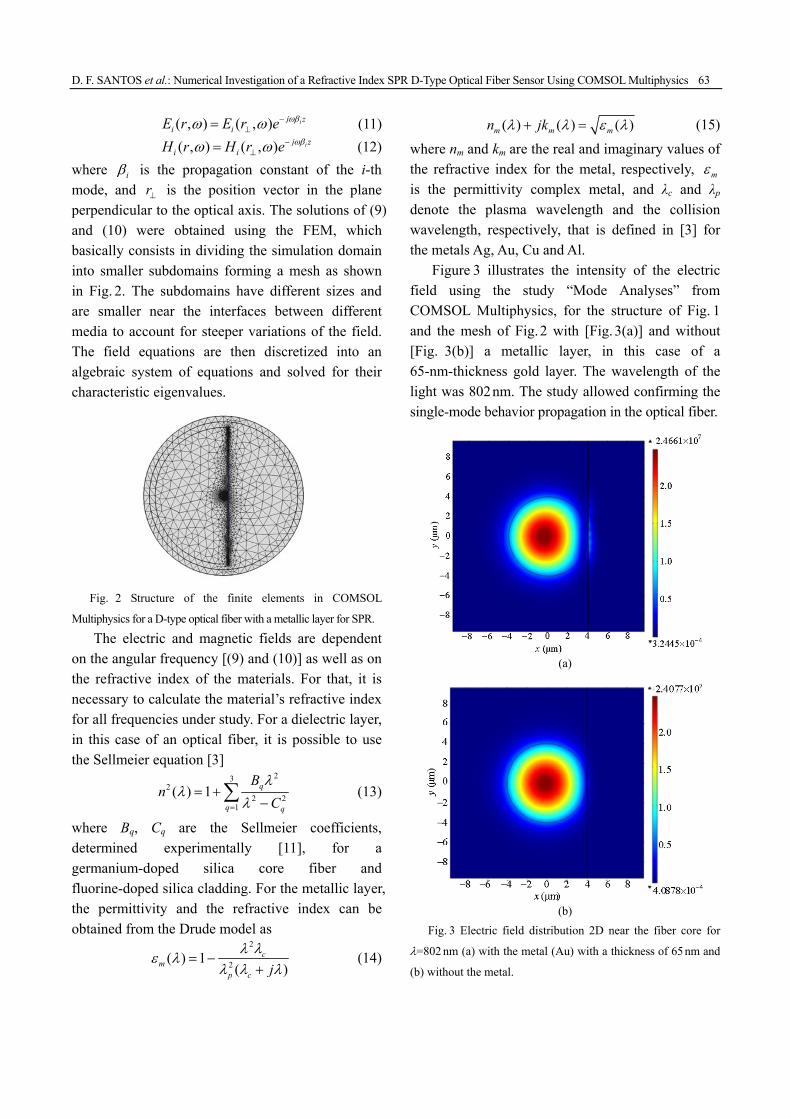
Figure 3 illustrates the intensity of the electric field using the study “Mode Analyses” from COMSOL Multiphysics, for the structure of Fig. 1

and the mesh of Fig. 2 with [Fig. 3(a)] and without [Fig. 3(b)] a metallic layer, in this case of a 65-nm-thickness gold layer. The wavelength of the

light was 802 nm. The study allowed confirming the single-mode behavior propagation in the optical fiber.

(a)

(b)

Fig. 3 Electric field distribution 2D near the fiber core for

=802 nm (a) with the metal (Au) with a thickness of 65 nm and

(b) without the metal.

Photonic Sensors

64

The 1D electrical field amplitude in the optical fiber is also shown in Figs. 4(a) and 4(b), with and without a metallic layer, respectively. Comparing both figures, it is possible to see the electric field intensity external to the fiber is stronger when using the metal.

2.4

2.2

2.0

1.8

1.6

1.4

1.2

1.0

0.8

0.6

0.4

0.2

0

103

Ele

ctri

c fi

eld

ampl

itud

e (V

/m)

0 2 4 6 8 10 12 14 16 18 20Arc length

(a)

2.4

2.2

2.0

1.8

1.6

1.4

1.2

1.0

0.8

0.6

0.4

0.2

0

103

Ele

ctri

c fi

eld

ampl

itud

e (V

/m)

0 2 4 6 8 10 12 14 16 18 20Arc length

(b)

Fig. 4 Electric field amplitude 1D across the fiber core for

=802 nm (a) with the metal (Au) with a thickness of 65 nm and

(b) without the metal.

Based on the simulation results provided by the COMSOL Multiphysics, one can compute the effective refractive index neff of the sensor [5] and from it the transmission coefficient T as a function of the wavelength , the external refractive index next and the thickness of the metal dm, according to the expression

eff ext 02 ( , , )ext( , , ) n n d k L

mT n d e . (16)

2.2 Transmission coefficient calculated using Fresnel laws

To verify that the method works properly, a

comparison was made with the implemented

algorithm in [12], which used Fresnel equations

applied to the structure in Fig. 1, allowing the

transmission intensity to be written (for four layers)

as / tan

ext 1234( , , ) ( ) cL rT n d r (17)

where 1234r is the reflective coefficient for four

layers as written 2

2

212 234

1234 212 2341

j k d

j k d

r r er

r r e

(18)

where the reflective coefficients for three layers and

two layers are, respectively 3

3

223 34

234 223 341

j k d

j k d

r r er

r r e

(19)

2 2

2 2

/ /

/ /i i j j

iji i j j

n k n kr

n k n k

(20)

where ki is the component of the wave vector of the

interface of the two layers of the sensor in the

direction z and is given as 2 2 1/ 20 1( sin )i ik k n n ,

where n1, n2, n3 and n4 represent the refractive

indices of the core, cladding, metal and the external

test medium, respectively.

Applying (16) and (17), it is possible to obtain

the results by the two different methods, as shown in Fig. 5. The behavior of the two methods was similar, having a difference between the transmission

coefficients and a small shift in the wavelength dips. We attributed this difference to the fact that in the Fresnel equations’ algorithm it is only considered

planar waves in a fairly symmetrical arrangement. On the other hand, when using the FEM, we considered the D-type fiber as a non-symmetrical

cylindrical waveguide, being able to model the inhomogeneous optical regions with a resolution of the cell size, resulting in a more accurate outcome.

In terms of the results and in what concerns the material thickness, the optimal point occurred when a layer with a thickness of 55 nm to 65 nm was used.

D. F. SANTOS et al.: Numerical Investigation of a Refractive Index SPR D-Type Optical Fiber Sensor Using COMSOL Multiphysics

65

Another way to test the efficiency of the

described procedure is to calculate the sensor

sensitivity (/RIU) as function of the different

refractive indices of the external environment. The

sensitivity for both methods is almost equal and is

close to 3150 nm/RIU [2].

Tailoring the simulation analysis in COMSOL

Multiphysics, it is possible to optimize the sensitivity,

transmission coefficient dip, wavelength operation

area, amongst others for a refractive index SPR

D-type optical fiber sensor. To decrease the depth of

the transmission coefficient dip and consequently

lower the sensitivity of the external medium, d can

be increased, as shown in Fig. 6.

Thickness of gold, 45 (nm)_COMSOL

Thickness of gold, 55 (nm)_COMSOL

Thickness of gold, 65 (nm)_COMSOL

Thickness of gold, 75 (nm)_COMSOL

Thickness of gold, 45 (n m)_Teorico

Thickness of gold, 55 (n m)_Teorico

Thickness of gold, 65 (n m)_Teorico

Thickness of gold, 75 (n m)_Teorico0.15

0.20

0.25

0.30

0.35

0.40

0.45

0.50

0.55

0.60

0.65

0.70

0.75

0.80

0.85

0.90

0.95

1.00

Tra

nsm

issi

on c

oeff

icie

nt

0.70 0.72 0.74 0.76 0.78 0.80 0 .82 0 .84 0 .8 6 0.8 8Waveleng th (μm)

Fig. 5 Transmission coefficient T as a function of the

wavelength and metallic layer thicknesses (Au), dm=0 m, L=

1 mm, next=1.3943 and =88.85.

From Figs. 5 and 6, it is possible to have a sensor that works for an area of operation near 820 nm, for

a metal thickness of 65 nm (Au).

In case another wavelength is required, one

possible solution is to apply an additional layer of a

dielectric with a high refractive index, such as

tantalum pentoxide (Ta2O5)[1–2], which simulation

results can be seen in Fig. 7 and compared with the

results presented in [2]. For different thicknesses of

Ta2O5, the transmission coefficient dip of the sensor

operation is not significantly altered being possible

to tailor the wavelength sensor operation [2].

d=0 μmd=0.5 μmd=1.0 μmd=2.0 μm

0.65

0.70

0.75

0.80

0.85

0.90

0.95

1.00

Tra

nsm

issi

on c

oeff

icie

nt

0.70 0.72 0.74 0.76 0.78 0.80 0.82 0.84 0.86 0.88 Wavelength (μm)

0.90 0.92 0.94

Fig. 6 Simulation of transmission coefficient of the sensor,

for different cladding thicknesses: in this simulation, the

thickness of the gold layer is 65 nm, and the refractive index of

the external environment is 1.3934.

T hickness of TAO, 20 nm

T hickness of TAO, 25 nm

T hickness of TAO, 30 nm

0

0.1

0.2

0.3

0.4

0.5

0.6

0.7

0.8

0.9

1.0

Tra

nsm

issi

on c

oeff

icie

nt

0.9 0 0 .92 0.940.76 0.7 8 0 .8 0 0 .82 0.84 0.86 0.88 Wavelen gth (μm)

Fig. 7 Simulation of transmission coefficient T of the sensor

for different thicknesses of the dielectric (Ta2O5): the thickness

of the gold is 65 nm and next=1.329.

3. Conclusions

Another method was demonstrated to study the

behavior of optical fiber sensors for refractive index

measurement based on SPR using COMSOL

Multiphysics, a commercial program that uses the

finite element method. The two simulations, one

with COMSOL Multiphysics and the other with

Fresnel’s equations, present a similar behavior. The

graphical interface of COMSOL Multiphysics

facilitates the simulation work, having no need to

Photonic Sensors

66

develop complex formulations. Also, it has the

ability to model inhomogeneous optical regions with

a resolution of the cell size and allows the analysis

of other parameters such as the intensity of magnetic

and electric field across the structure [13].

COMSOL Multiphysics permits in a graphical

environment more accurate and realistic results than

traditional approaches, although at the expense of

longer running time.

It was also possible to demonstrate the use of

COMSOL Multiphysics to improve the performance

of a refractive index SPR D-type optical fiber sensor,

where the characteristics of the material layers, in

terms of the type and thickness, and the residual

fiber cladding thickness are optimized.

Open Access This article is distributed under the terms

of the Creative Commons Attribution License which

permits any use, distribution, and reproduction in any

medium, provided the original author(s) and source are

credited.

References [1] B. Lee, S. Roh, and J. Park, “Current status of micro-

and nano-structured optical fiber sensors,” Optical Fiber Technology, vol. 15, no. 3, pp. 209–221, 2009.

[2] R. Slavik, J. Homola, J. Ctyroký, and E. Brynda, “Novel spectral fiber optic sensor based on surface plasmon resonance,” Sensors and Actuators B: Chemical, vol. 74, no. 1–4, pp. 106–111, 2001.

[3] A. K. Sharma and B. D. Gupta, “On the performance of different bimetallic combinations in surface plasmon resonance based fiber optic sensors,” Journal of Applied Physics, vol. 101, no. 9, p. 093111-1– 093111-6, 2007.

[4] E. Anemogiannis, E. N. Glytsis, and T. K. Gaylord, “Transmission characteristics of long-period fiber gratings having arbitrary azimuthal/radial refractive index variations,” Journal of Lightwave Technology, vol. 21, no. 1, pp. 218–227, 2003.

[5] Y. Al-Qazwini, P. T. Arasu, and A. S. M. Noor, “Numerical investigation of the performance of an SPR-based optical fiber sensor in an aqueous environment using finite-difference time domain,” in Proc. 2011 2nd International Conference on Photonics, Oct. 17–19, vol. 1, pp. 1–4, 2011.

[6] B. Culshaw, F. Muhammad, R. Van Ewyk, G. Stewart, S. Murray, D. Pinchbeck, et al., “Evanescent wave methane detection using optical fibers,” Electronics Letters, vol. 28, no. 24, pp. 2232–2234, 1992.

[7] F. M. Araújo, L. A. Ferreira, J. L. Santos, and F. Farahi, “Temperature and strain insensitive bending measurements with D-type fiber Bragg gratings,” Measurement Science and Technology, vol. 12, no. 7, pp. 829–833, 2001.

[8] M. H. Chiu, S. F. Wang, and R. S. Chang, “D-type fiber biosensor based on surface-plasmon resonance technology and heterodyne interferometry,” Optics Letters, vol. 30, no. 3, pp. 233–235, 2005.

[9] Y. Chen and H. Ming, “Review of surface plasmon resonance and localized surface plasmon resonance sensor,” Photonics Sensors, vol. 2, no. 1, pp. 37–49, 2012.

[10] M. Fliziani and F. Maradei, “Edge element analysis of complex configurations in presence of shields,” IEEE Transactions on Magnetics, vol. 33, no. 2, pp. 1548–1551, 1997.

[11] A. Méndez and T. F. Morse, Specialty Optical Fibers Handbook. San Diego, California: Academic Press, 2007, pp. 39–40.

[12] M. H. Chiu, C. H. Shih, and M. H. Chi, “Optimum sensitivity of single-mode D-type optical fiber sensor in the intensity measurement,” Sensors and Actuators B: Chemical, vol. 123, no. 2, pp. 1120–1124, 2007.

[13] D. Christensen and D. Fowers, “Modeling SPR sensors with the finite-difference time-domain method,” Biosensors & Bioelectronics, vol. 11, no. 6, pp. 677–684, 1996.