numerical examination of flow field characteristics and

Numerical Examination of Flow Field Characteristics

and

Fabri Choking of 2D Supersonic Ejectors

A Thesis

Presented to the Faculty of

California Polytechnic State University

San Luis Obispo

In Partial Fulfillment of the Requirements

For the Degree of Master of Science

In Aerospace Engineering

by

Brett G. Morham

June 2010

ii

© 2010 Brett G Morham

ALL RIGHTS RESERVED

iii

COMMITTEE MEMBERSHIP

Title: Numerical Examination of Flow Field Characteristics and Fabri Choking of 2D Supersonic Ejectors

Author: Brett G Morham Date Submitted: June 2010 Advisor and Committee Chair: Dr. Dianne DeTurris Faculty Committee Member: Dr. David Marshall Faculty Committee Member: Dr. William Durgin Industry Committee Member: Ryan Gist

iv

ABSTRACT Numerical Examination of Flow Field Characteristics and Fabri Choking

of 2D Supersonic Ejectors

Brett Morham

An automated computer simulation of the two-dimensional planar Cal Poly Supersonic

Ejector test rig is developed. The purpose of the simulation is to identify the operating

conditions which produce the saturated, Fabri choke and Fabri block aerodynamic flow

patterns. The effect of primary to secondary stagnation pressure ratio on the efficiency of

the ejector operation is measured using the entrainment ratio which is the secondary to

primary mass flow ratio.

The primary flow of the ejector is supersonic and the secondary (entrained) stream enters

the ejector at various velocities at or below Mach 1. The primary and secondary streams

are both composed of air. The primary plume boundary and properties are solved using

the Method of Characteristics. The properties within the secondary stream are found

using isentropic relations along with stagnation conditions and the shape of the primary

plume. The solutions of the primary and secondary streams iterate on a pressure

distribution of the secondary stream until a converged solution is attained. Viscous

forces and thermo-chemical reactions are not considered.

For the given geometry the saturated flow pattern is found to occur below stagnation

pressure ratios of 74. The secondary flow of the ejector becomes blocked by the primary

plume above pressure ratios of 230. The Fabri choke case exists between pressure ratios

of 74 and 230, achieving optimal operation at the transition from saturated to Fabri

choked flow, near the pressure ratio of 74. The case of optimal expansion yields an

entrainment ratio of 0.17. The entrainment ratio results of the Cal Poly Supersonic

Ejector simulation have an average error of 3.67% relative to experimental data. The

accuracy of this inviscid simulation suggests ejector operation in this regime is governed

by pressure gradient rather than viscous effects.

v

Acknowledgments

I must thank my family, my friends, and my thesis committee. My parents Eric

and Olga Morham and my brothers Kyle and Sean have provided endless encouragement,

motivation and generosity. Without my family, none of this would have been possible.

My friends, especially Rae Boghossian, have offered unlimited patience and optimism.

Without this balance, I would never have been able to complete this project.

I must acknowledge Dr. DeTurris for inspiring me and opening my eyes to the

world of hypersonics and this project. Dr. DeTurris has kept me on track and motivated,

selflessly allocating time for support and advising. Ryan Gist has acted as a mentor

before and throughout this project. Ryan and his colleagues at Rocketdyne, especially

Bill Follett, have provided invaluable perspective. Thank you to Joey Sanchez and

Martin Popish for having faith in this project and coming on board, keeping the project

alive. Also, thank you Paul Riley for providing a working MOC nozzle code which acted

as a backbone for the simulation.

I would like to thank my thesis committee as a whole; Dr. DeTurris, Ryan Gist,

Dr. Durgin and Dr. Marshall. Thank you for taking the time and providing the insight to

make this thesis what it now is.

Finally, I dedicate this work to Mark Waters. He was a true mentor to the world

of propulsion. The influence of his passion and dedication to the field is immeasurable.

vi

Table of Contents List of Figures.................................................................................................. vii Nomenclature ................................................................................................... ix 1 Introduction ................................................................................................. 1

1.1 Geometry Classification....................................................................... 1 1.2 Flow Composition Classification ......................................................... 3 1.3 Flow Velocity Classification ................................................................ 4 1.4 Objectives............................................................................................ 4 1.5 Applications......................................................................................... 5

2 Literature Review ...................................................................................... 12 2.1 Seminal Works .................................................................................. 12

2.1.1 Fabri .......................................................................................... 12 2.1.2 Emanuel ..................................................................................... 15 2.1.3 Addy .......................................................................................... 17

2.2 Supplemental Analysis Approaches ................................................... 19 2.2.1 Shear Layers .............................................................................. 19 2.2.2 Reacting Flow ............................................................................ 20 2.2.3 Lobed Ejectors ........................................................................... 20 2.2.4 Computational Fluid Dynamics .................................................. 20

2.3 Motivational Works ........................................................................... 21 2.3.1 Foster10 ...................................................................................... 21 2.3.2 Gist4 ........................................................................................... 23

3 Methodology ............................................................................................. 25 3.1 Assumptions ...................................................................................... 26 3.2 Primary Plume Calculation Method.................................................... 26

3.2.1 Method of Characteristics Interior Point Calculation .................. 28 3.2.2 Method of Characteristics Direct Wall Point Calculation ............ 32 3.2.3 Method of Characteristics Free Pressure Boundary Point Calculation ................................................................................................ 34

3.3 Secondary Stream Calculation Method............................................... 37 3.3.1 Mach number solution................................................................ 38 3.3.2 Isentropic values ........................................................................ 39

3.4 Iteration Scheme ................................................................................ 40 3.4.1 Relaxation Factors...................................................................... 41

3.5 Entrainment Ratio Calculation ........................................................... 41 4 Results of the CPSE Simulation................................................................. 44

4.1 Saturated Supersonic Flow Pattern ..................................................... 45 4.2 Fabri Choke Supersonic Flow Pattern ................................................ 49 4.3 Blocked Flow Pattern......................................................................... 52

5 Comparisons to Previous Work.................................................................. 55 6 Conclusions ............................................................................................... 62 7 Future Work .............................................................................................. 64 8 References ................................................................................................. 65 9 Appendix................................................................................................... 68

vii

List of Figures Figure 1-1 Top and front view of an axisymmetric ejector ..............................................1 Figure 1-2 Top and front view of a two-dimensional planar ejector ................................2 Figure 1-3 Side and front view of a planar lobed ejector2.................................................3 Figure 1-4 Ramjet operation cycle ..................................................................................6 Figure 1-5: Effects of Mach number of efficiency of propulsion systems4........................7 Figure 1-6 X-43 Hypersonic test vehicle 3-view5 ............................................................8 Figure 1-7 Schematic of the multistage operation for the X-43 test flight6 ......................9 Figure 1-8 SR-71 turbine based combined cycle vehicle 3-view7 ....................................9 Figure 1-9 Turbine based combined cycle engine integration9 .......................................10 Figure 1-10 Concept vehicle incorporating a rocket based combined cycle

propulsion system10 ...............................................................................................11 Figure 2-1 Secondary flow achieves critical Mach number during the Fabri choke

condition ...............................................................................................................14 Figure 2-2 The secondary flow entering the mixing chamber is sonic during the

saturated flow pattern ............................................................................................ 14 Figure 2-3 The primary flow becomes subsonic during the subsonic flow pattern.........15 Figure 2-4 The Cal Poly Supersonic Ejector .................................................................22 Figure 2-5 The variation between ideal and actual primary plume expansion4................25 Figure 2-6 Growth of primary plume from ideal to actual size due to empirical

correction factor10 ..................................................................................................25 Figure 3-1 Definition of primary plume using Method of Characteristics......................27 Figure 3-2 Method of Characteristics unit process for an interior point25 .......................28 Figure 3-3 Definition of angles used in Method of Characteristics ................................30 Figure 3-4 Method of Characteristics unit process for a symmetry point25 ....................31 Figure 3-5 Method of Characteristics unit process for a wall point25 ..............................33 Figure 3-6 Method of Characteristics unit process for free pressure boundary

point ......................................................................................................................35 Figure 3-7 Components of the velocity vector along the free pressure boundary

streamline ..............................................................................................................37 Figure 3-8 The Mach number of secondary flow using isentropic area relations............38 Figure 4-1 Dimensioned top view of the CPSE test apparatus4......................................45 Figure 4-2 CPSE simulation of the Mach number distribution of a saturated flow

pattern ...................................................................................................................46 Figure 4-3 CPSE simulation of the static pressure distribution of a saturated flow

pattern ...................................................................................................................48 Figure 4-4 CPSE simulation of the Mach number distribution of a Fabri choke

supersonic flow pattern..........................................................................................50 Figure 4-5 CPSE simulation of the static pressure distribution of a Fabri choke

supersonic flow pattern..........................................................................................51 Figure 4-6 CPSE simulation of the Mach number distribution of a blocked flow

pattern ...................................................................................................................53 Figure 4-7 CPSE simulation of the static pressure distribution of a blocked flow

pattern ...................................................................................................................54 Figure 5-1 Nitrogen condensation plume in the mixing chamber at a pressure

ratio of 954.............................................................................................................56

viii

Figure 5-2 Methane and Oxygen thruster fired at a pressure ratio of 2010 .......................56 Figure 5-3 Video frame and superimposed shock structure from cold flow tests4 ...........57 Figure 5-4 Mach Number and Streamlines from CFD Model30 .....................................58 Figure 5-5 Entrainment ratio calculations using empirical correction factor for

plume size4 ............................................................................................................59 Figure 5-6 Comparison of CPSE computer code to experimental data and

empirical predictions .............................................................................................61

ix

Nomenclature a Speed of Sound [ft/s] A Area [ft2],[in2] C Characteristic Curve (Mach Line) - h Ejector height [ft],[in] Isp Specific Impulse (s) K Relaxation Factor - Kexpand Plume Expansion Correction Factor - M Mach Number - m Mass Flow Rate [lbm/s] P Stagnation Pressure [lbf/ft2] p Static Pressure [lbf/ft2] Q,R,T Coefficients in Finite Difference Equations - R Universal Gas Constant [lbf-ft/lbm°R] T Temperature [°F, °R] tb Primary Nozzle Base Thickness [ft],[in] u Transverse Velocity Component [ft/s] v Streamwise Velocity Component [ft/s] V Total Velocity [ft/s] x Streamwise Position From Primary Throat [ft],[in] y Streamwise Position from Centerline [ft],[in] Mach Angle [deg], [rad] Entrainment Ratio = PS mm - γ Ratio of Specific Heats - ε Nozzle Expansion Ratio = Aexit/A* - Slope Tangent to Characteristic Line - ρ Density (slug/ft3) Streamline Flow Angle [deg], [rad] Subscripts 0 Stagnation Condition, Streamline Condition for Method of

Characteristics 1 Known Property of Point 1 in Method of Characteristic Calculation 2 Known Property of Point 2 in Method of Characteristic Calculation 3 Known Property of Point 3 in Method of Characteristic Calculation 4 Method of Characteristics Point of Interest + Positive Left Running Characteristic (Mach Line) - Negative Right Running Characteristic (Mach Line) i Arbitrary index denoting corresponding position P Primary Stream S Secondary Stream Superscripts * Critical Point (sonic throat)

1

1 Introduction Ejectors use a high velocity, high pressure flow to energize a low pressure low velocity

flow. The high pressure driving flow is termed the primary flow. The low pressure flow

being energized is the secondary flow. The area in which the primary and secondary

flows interact is termed the mixing chamber or mixing duct. The conditions which

dictate the interactions between the primary and secondary streams are many; however,

the stagnation pressure ratio between the primary and secondary streams is the most

referenced parameter. Since the purpose of an ejector is for the primary flow to entrain

the secondary flow, the secondary to primary mass flow ratio, also called the entrainment

ratio ( ), is a typical measure of ejector performance. Historically, ejectors have been

used for industrial applications such as vacuum packaging, pumping chemical lasers, and

thrust augmentation in aircraft turbine engines1. Ejectors are classified by their

geometry, flow composition, and flow velocities.

1.1 Geometry Classification Typical ejector geometries include axisymmetric, two-dimensional and lobed

configurations. Axisymmetric ejectors have the primary and secondary streams

concentrically arranged. Typically the primary flow is in the center and the secondary

flow is entrained through an outer passage which is bounded by the primary nozzle and

the duct wall. A basic axisymmetric ejector is shown in Figure 1-1.

Figure 1-1 Top and front view of an axisymmetric ejector

The top view of the axisymmetric ejector shows the duct walls extending far beyond the

primary nozzle which is centrally located. The primary nozzle produces the high energy

Duct Wall

Duct Wall

Duct Wall

Primary Nozzle Primary Stream

Secondary Stream

Secondary Stream Primary Nozzle

Mixing Chamber

2

flow which entrains the fluid from the secondary stream. A long outer duct is required to

promote complete mixing of the primary and secondary streams. The mixing chamber is

the area bounded by the end of the primary nozzle in the stream wise direction and the

end of the duct. The primary and secondary streams interact in the mixing chamber

before exiting the ejector. The mixing chamber is also often called the mixing duct.

Two-dimensional planar ejectors generally have one line of symmetry on the centerline

of the primary plume. A generic two-dimensional planar ejector is shown in Figure 1-2.

Figure 1-2 Top and front view of a two-dimensional planar ejector

Similar to the axisymmetric configuration, the primary nozzle is in the center,

symmetrically entraining secondary flow. The primary and secondary flows react in the

mixing chamber beyond the primary nozzle before exiting the duct. While the nozzle of

an axisymmetric ejector is surrounded on all sides by the secondary flow; planar ejectors

are bounded on the top and bottom by upper and lower duct walls. The primary nozzle

extends from the lower duct wall to the upper duct wall. The secondary flow is not

entrained above or below the primary flow. The planar configuration has reduced

secondary flow area compared to axisymmetric ejectors of similar external dimensions.

With the upper and lower walls acting as structure for planar ejectors, this geometry has

configuration and packaging benefits.

Duct Wall

Primary Nozzle

Secondary Stream

Primary Stream

Secondary Stream

Mixing Chamber

Duct Wall

Primary Nozzle

Upper and Lower Duct Walls

3

Lobed ejectors have flower shaped primary nozzles and various outer duct shapes. The

purpose of the elaborate geometries is to promote mixing of the primary and secondary

stream. Lobed ejectors may be axisymmetric or planar. A planar lobed ejector is shown

in Figure 1-3.

Figure 1-3 Side and front view of a planar lobed ejector2

The more elaborate primary nozzle geometry increases the surface area between the

primary and secondary flows for more efficient mixing of the streams.

1.2 Flow Composition Classification The gas properties of the primary and secondary streams have a large influence on the

performance of an ejector. It is common to analyze ejectors which have primary and

secondary streams of similar chemical composition. The basic air-air ejector analysis

does not require consideration of chemical interaction. However, chemical and thermo-

chemical reactions occur between the streams when the flows have different properties

and compositions. These different flow compositions arise depending on the ejector

application.

Changing the composition of the flows adds the complexity of chemistry based

interactions between the primary and secondary stream. The streams may also be of

different phase. The presence of liquid droplets or vapors can cause distinct flow

phenomenon1. The amount of liquid present in the flow also influences the performance

4

of the ejector and will change the optimal geometric configuration. Multiphase ejector

analysis is important for heating and cooling applications.

An area of thermo-chemically reactive flow which has a propulsion application is that of

a fuel rich combusting primary plume3. In this case there is an exchange of chemical,

aerodynamic and thermal energy between the primary and secondary streams. The fuel

rich primary plume is aided in combustion by the oxygen being entrained within the

secondary flow. The transition from stored chemical energy to flow velocity achieved by

this system makes it ideal for aerospace propulsion applications.

1.3 Flow Velocity Classification Ejectors have primary or secondary flows which can be subsonic or supersonic. Subsonic

ejectors such as induction pumps have lower primary to secondary stagnation pressure

ratios. Neither the primary nor the secondary flow of a subsonic ejector ever achieves a

sonic or supersonic condition.

Supersonic ejectors have higher primary to secondary stagnation pressure ratios. Choked

flow in the throat of the primary nozzle due to a high chamber pressure is required to

achieve supersonic primary flow. The primary flow accelerates to supersonic Mach

numbers in the expanding area of the primary nozzle. The supersonic primary flow of an

ejector is commonly referred to as the primary plume. The secondary flow velocity

within a supersonic ejector varies. The secondary flow may enter at subsonic or

supersonic Mach numbers. The secondary stream may exit the duct subsonic, sonic or

supersonic, regardless of the inlet Mach number. The performance of the streams is

determined by ejector geometry, primary to secondary stagnation pressure ratio, the

ambient pressure at the ejector exit and the gas properties of the flows.

1.4 Objectives The objective of developing the CPSE analysis method is to provide reliable and rapid

approximations of a two-dimensional supersonic ejector with non-reacting flow of similar

5

composition without empirical correction factors. The simulation provides insight into

the relationship of stagnation pressure ratio and entrainment ratio within the ejector. The

simulation will also give medium fidelity approximations of the properties within the

primary and secondary flows. This tool can be used to run many cases before time

intensive CFD or experimental analysis is performed for final high fidelity analysis.

The ejector serving as the topic for this analysis is two-dimensional planar in geometry.

The primary and secondary flows are considered similar in gas composition and

temperature. The similar flows do not have significant chemical interaction between the

streams. The primary plume is high supersonic with flows up to Mach 5. The secondary

inlet stream velocity varies from no flow to sonic. The primary and secondary streams do

not have water droplets or condensation within the gases. Neither of the plumes undergo

combustion at any stage of operation.

A computer automated analysis method has been developed to simulate a two-

dimensional planar air-air ejector for comparison with the Cal Poly Supersonic Ejector.

This analysis tool is termed the CPSE simulation. The primary plume is described using

the two-dimensional Method of Characteristics (MOC). The secondary stream is

analyzed using isentropic relations. The interaction between the streams and the ejector

surfaces are assumed to be inviscid. Thermo-chemical reactions between the streams are

not considered.

The CPSE simulation is to be validated against experimental data obtained from the Cal

Poly Supersonic Ejector experimental test rig. Recorded pressure ratio and entrainment

ratio values are used as the standard for comparison. Once the simulation has been

shown to correspond to this set up, many planar configurations can be simulated with the

CPSE code within the given assumptions.

1.5 Applications The primary application of interest for this study is the fusion of air augmented rocket

technology with ramjet vehicles. A ramjet is a high speed propulsion technology which

6

requires supersonic flight velocities in order to operate. Traditional reciprocating and jet

engines use pistons and turbo-machinery to compress air to a level where it can be

combusted. The combustion products then expand, creating mechanical energy or thrust.

Ramjets do not require mechanical machinery for operation. Instead, the geometry of the

ramjet inlet is designed to induce a shock train, terminating in a normal shock, which

causes the air to decelerate from supersonic to subsonic speeds. Fuel is introduced into

the subsonic high pressure air and combusted. The combustion products expand out of

the ramjet nozzle supersonically, creating thrust. A subset of the ramjet system is the

supersonic combustion ramjet, scramjet. The basic principles of ramjet operation hold

true for scramjets; however, the incoming flow does not experience a normal shock and

remains supersonic throughout the entire process. Figure 1-4 illustrates the fundamental

ramjet propulsion cycle.

Figure 1-4 Ramjet operation cycle

Due to the high speeds required for ramjets to operate, their flight regime is limited.

Figure 1-5 shows the variation of efficiency with Mach number for various propulsion

systems.

Inlet (M>1)

Shock Induced Compression

(to M<1) Expansion of Exhaust

(M>1) Fuel Injection Combustion

7

Figure 1-5: Effects of Mach number of efficiency of propulsion systems4

Figure 1-5 illustrates that there is a gap at low Mach numbers where a pure ramjet cannot

operate. Turbojets are able to operate in the supersonic regime; though, the efficiency is

greatly reduced beyond Mach 1. Rockets are able to operate across the range of Mach

numbers; yet, they operate very inefficiently in all conditions. Ramjets and scramjets are

able to operate at Mach numbers beyond those of jet engines at higher efficiencies than

rockets. However, in order to operate a ramjet, the system must be accelerated to

supersonic speeds. Ramjets operate most efficiently between Mach 2.0 and Mach 5.04.

Vehicles operating beyond Mach 5 may be accelerated by auxiliary booster vehicles or

utilize combined cycle systems. Combined cycle propulsion systems use turbojets or

rockets to accelerate hypersonic vehicles to a flight condition where the ramjet cycle can

operate.

The X-43 scramjet test vehicle shown in Figure 1-6 was launched from a modified

Pegasus missile which had been dropped off a B-52 in order to achieve the required flight

conditions for operation.

8

Figure 1-6 X-43 Hypersonic test vehicle 3-view5

The X-43 is an example of a multi-stage vehicle. The B-52 which lifted both the Pegasus

missile and the X-43 is considered the first stage of the system. The Pegasus which

dropped off the wing of the B-52 and accelerated the X-43 to operating speeds was the

second stage. The X-43 itself became the final stage once it departed from the Pegasus.

A schematic of the multistage operation of the X-43 system is shown in Figure 1-7.

9

Figure 1-7 Schematic of the multistage operation for the X-43 test flight6

The SR-71 Blackbird aircraft shown in Figure 1-8 has engines which switch to ramjet

propulsion from jet propulsion at high Mach numbers. The SR-71’s J58 turbo-ramjet

engines are an example of a combined cycle propulsion system.

Figure 1-8 SR-71 turbine based combined cycle vehicle 3-view7

The SR-71aircraft takes off and accelerates using jet engines. Once the vehicle switches

to ramjet mode, no components of the system are dropped or discarded. The vehicle can

then switch back to turbojet mode for lower flight speeds and landing. This integrated

combined cycle propulsion system is an example of a turbine based combined cycle,

10

TBCC. TBCC systems incorporate the high efficiency of turbine engines at low Mach

numbers and the ability of Ramjets to operate at high Mach numbers.

Recently TBCC systems have received renewed attention. Lockheed Martin responded

to Darpa’s Falcon program request for a hypersonic flight vehicle with horizontal takeoff

and landing capability with the Blackswift hypersonic cruise vehicle (HCV). Blackswift

utilized shared inlets and nozzles for the turbine and ramjet propulsion systems. The

demonstrator would have been able to takeoff from a runway, accelerate to Mach 6 under

its own power and maneuver at hypersonic speeds before landing. It was reported that

the required funding was not supplied and the project was cancelled by the year 2009.

The Falcon program is continuing structural and aerodynamic development for

hypersonic vehicles using unpowered gliders launched with Minotaur booster rockets8.

A NASA concept designed to test TBCC systems is shown in Figure 1-9. TBCC

systems are limited in that they cannot operate at very high Mach numbers or at very high

altitudes due to lack of atmospheric density which is required to operate air-breathing

propulsion systems. These restrictions limit space and orbital related applications of

TBCC systems.

Figure 1-9 Turbine based combined cycle engine integration9

Currently, vehicles such as the Space Shuttle require multiple stages to reach Earth’s

orbit. These rocket based systems require multiple stages because the fuel and the

oxidizer for all the stages must be carried in large tanks which are discarded throughout

the mission. By reducing the oxidizer storage requirements, it may be possible to create a

vehicle that requires only a single stage to orbit, SSTO.

11

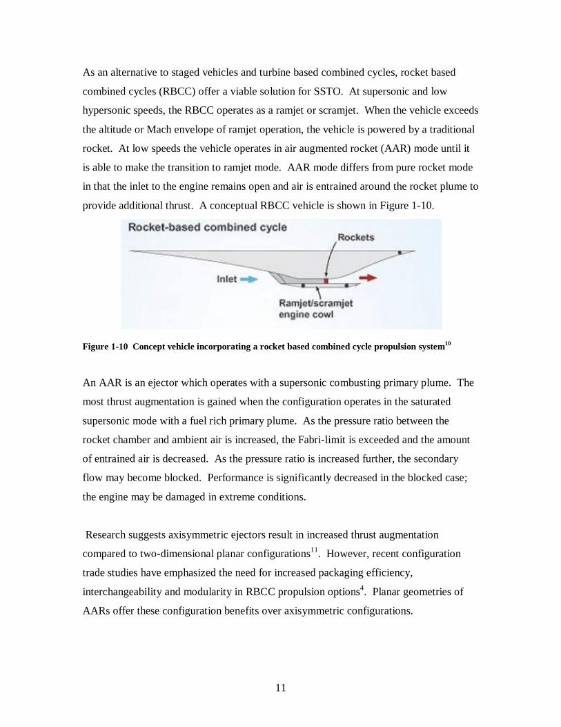
As an alternative to staged vehicles and turbine based combined cycles, rocket based

combined cycles (RBCC) offer a viable solution for SSTO. At supersonic and low

hypersonic speeds, the RBCC operates as a ramjet or scramjet. When the vehicle exceeds

the altitude or Mach envelope of ramjet operation, the vehicle is powered by a traditional

rocket. At low speeds the vehicle operates in air augmented rocket (AAR) mode until it

is able to make the transition to ramjet mode. AAR mode differs from pure rocket mode

in that the inlet to the engine remains open and air is entrained around the rocket plume to

provide additional thrust. A conceptual RBCC vehicle is shown in Figure 1-10.

Figure 1-10 Concept vehicle incorporating a rocket based combined cycle propulsion system10

An AAR is an ejector which operates with a supersonic combusting primary plume. The

most thrust augmentation is gained when the configuration operates in the saturated

supersonic mode with a fuel rich primary plume. As the pressure ratio between the

rocket chamber and ambient air is increased, the Fabri-limit is exceeded and the amount

of entrained air is decreased. As the pressure ratio is increased further, the secondary

flow may become blocked. Performance is significantly decreased in the blocked case;

the engine may be damaged in extreme conditions.

Research suggests axisymmetric ejectors result in increased thrust augmentation

compared to two-dimensional planar configurations11. However, recent configuration

trade studies have emphasized the need for increased packaging efficiency,

interchangeability and modularity in RBCC propulsion options4. Planar geometries of

AARs offer these configuration benefits over axisymmetric configurations.

12

It is imperative to understand the conditions which lead to optimum AAR performance

and how to avoid reduced performance and engine damage. In the following sections the

operation of planar ejectors across a range of pressure ratios is examined to better

understand the factors which determine the performance of air augmented rockets.

2 Literature Review Countless works have been compiled regarding the interactions occurring within

supersonic air to air ejectors. These works have provided knowledge, methods and

motivation for the analysis to follow.

2.1 Seminal Works Fabri12,13 defined the operating conditions of an air-air ejector with supersonic primary

flow which causes aerodynamic choking of the secondary flow. Emanuel18 compared

Fabri’s method with the one-dimensional method and proposed a hybrid method. Addy14

expanded on Fabri’s method, introducing various degrees of viscous interaction and a

transient analysis. These methods share the trait that they evaluate ejector performance

by total analysis from inlet to exit.

2.1.1 Fabri Fabri et al12,13 systematically investigate operating conditions of an air to air jet ejector

with high pressure supersonic primary flow and low pressure induced secondary flow.

The configuration used for the analysis is cylindrical and axisymmetric. Fabri defines

several aerodynamic flow patterns of ejector operation in order of decreasing primary

stagnation pressure.

Fabri’s analysis is of a cylindrical ejector with the primary nozzle aligned with the

cylinder axis. This analysis does not take into account viscosity or diffusion between the

streams. A correction is made for the friction between the secondary flow and the duct

wall. The primary and secondary flows are assumed to be the same gas which is treated

as a perfect gas. The primary flow is low supersonic at the exit of the primary nozzle.

The velocity of secondary flow at the entrance to the mixing chamber varies. At the exit

of the mixing chamber, the flows have uniform pressure which matches the exit

condition.

13

The primary flow is solved using the classical quasi-one-dimensional approach.

However, Fabri suggests that the Method of Characteristics be utilized when the primary

plume area is expanding because the quasi-one-dimensional approach requires correction

factors to predict the area of the primary plume. The values of the inlet conditions to the

mixing chamber of the primary and secondary streams are used to solve the conservation

equations. The outlet condition is the sum of the primary and secondary inlet mass flow,

momentum and energy with the condition of uniform ambient pressure imposed.

Although the interaction between the streams is inviscid, a correction for pressure loss

due to wall friction is imposed. Fabri’s analysis provides some insight into the flow

phenomenon occurring within the ejector from experimental trials. Fabri’s analysis

method does not yield the properties of the streams within the flow. Fabri defines three

flow patterns which classify different regimes of supersonic ejector operation. The flow

may be termed Fabri choke supersonic, saturated supersonic or subsonic. The Fabri

choke and saturated conditions are both special cases of the supersonic case. If the duct

is suffiently short the mixed case may occur where the secondary stream does not achieve

aerodynamic choking before the duct exit.

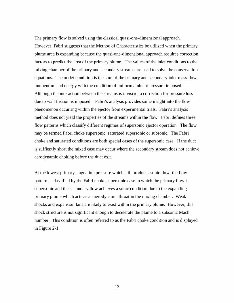
At the lowest primary stagnation pressure which still produces sonic flow, the flow

pattern is classified by the Fabri choke supersonic case in which the primary flow is

supersonic and the secondary flow achieves a sonic condition due to the expanding

primary plume which acts as an aerodynamic throat in the mixing chamber. Weak

shocks and expansion fans are likely to exist within the primary plume. However, this

shock structure is not significant enough to decelerate the plume to a subsonic Mach

number. This condition is often referred to as the Fabri choke condition and is displayed

in Figure 2-1.

14

Figure 2-1 Secondary flow achieves critical Mach number during the Fabri choke condition

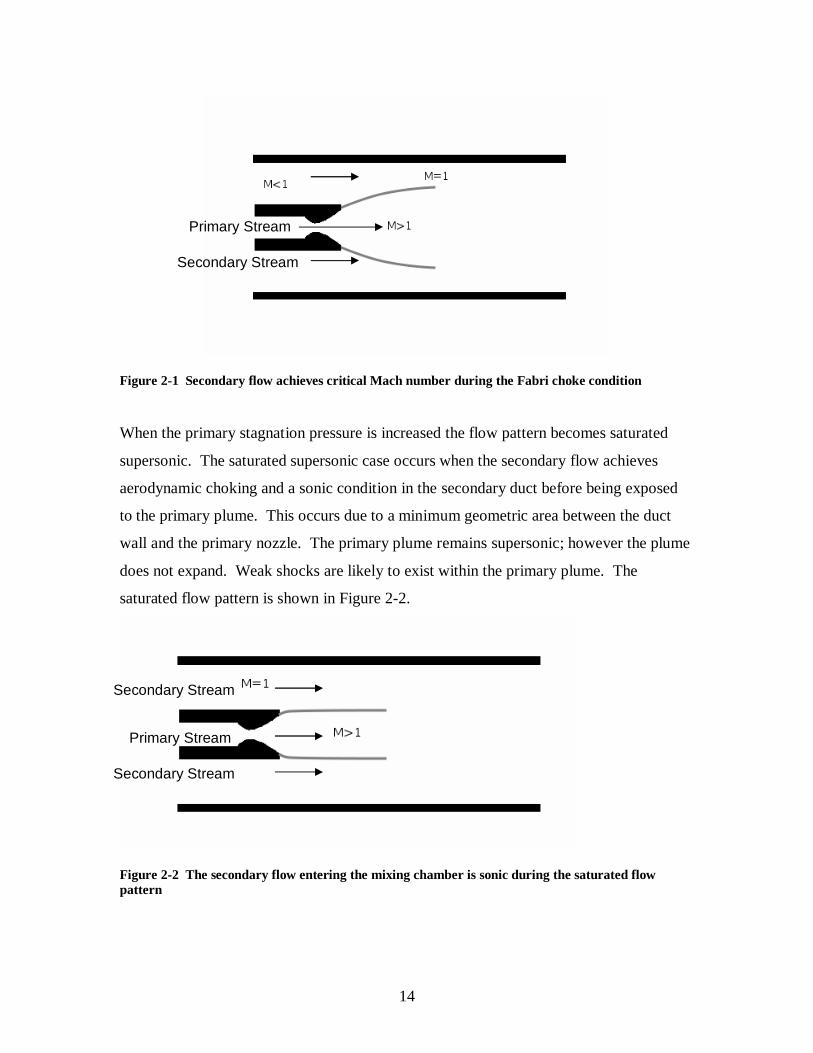
When the primary stagnation pressure is increased the flow pattern becomes saturated

supersonic. The saturated supersonic case occurs when the secondary flow achieves

aerodynamic choking and a sonic condition in the secondary duct before being exposed

to the primary plume. This occurs due to a minimum geometric area between the duct

wall and the primary nozzle. The primary plume remains supersonic; however the plume

does not expand. Weak shocks are likely to exist within the primary plume. The

saturated flow pattern is shown in Figure 2-2.

Figure 2-2 The secondary flow entering the mixing chamber is sonic during the saturated flow pattern

Secondary Stream

Primary Stream

Secondary Stream

Secondary Stream

Primary Stream

15

The flow pattern with the lowest primary stagnation pressure which still induces

secondary flow is the subsonic case. The subsonic condition occurs when the primary

pressure is low enough that the back pressure from the ambient exit condition forces a

strong shock train to form in the primary plume which terminates in a normal shock.

This shock structure decelerates the primary flow to subsonic velocities. The secondary

flow is then entrained by a subsonic primary flow and the streams become fully mixed

before exiting the duct. This is illustrated in Figure 2-3.

Figure 2-3 The primary flow becomes subsonic during the subsonic flow pattern

Fabri’s method utilizing conservation of energy and momentum to solve for the

aerodynamic flow patterns for each condition provides some insight into the interactions

between the flows. However, Fabri’s method does not accurately provide properties of

the flow within the mixing chamber. Although the method is inviscid, corrections are

made for the friction from the duct walls and the thickness of the lip of the primary

nozzle. Later analyses2, 3, 11, 14, 15,16 reject the nozzle lip thickness correction and

implement a mixing layer between the primary and secondary streams.

2.1.2 Emanuel Emanuel18 compares the one-dimensional analysis of supersonic air to air ejectors to

Fabri’s inviscid method. The one-dimensional calculations are typically used for

parametric analyses due to the ease of implementation. In this method, all parameters

are fixed, besides a single independent variable, typically the inlet Mach number. The

flows are mixed in a constant area mixer. The ejected flows may be supersonic, or

Shock Structure

Secondary Stream

Secondary Stream

Primary Stream

16

subsonic. The one-dimensional method provides little insight into the flow phenomenon

occurring within the ejector. Due to the amount of properties required to run the

calculations, a large number of assumptions and apriori knowledge is required. Accurate

properties of the streams within the mixing chamber are not provided by this method.

The one-dimensional ejector model requires the assumption of constant area mixing or

constant pressure mixing. It is possible for both assumptions to be applied. The constant

area assumption requires the mixing area to remain unchanged in the stream wise

direction. The constant pressure assumption implies the primary and secondary pressures

are equal entering the mixing chamber. Further, it is assumed that the primary and

secondary flows are fully mixed at the exit of the ejector duct.

The primary and secondary flows are characterized by their stagnation conditions as well

as the Mach number and area at the entrance to the mixing chamber. From these values,

properties such as velocity and mass flow rate can be calculated. A control volume

approach with conversation of mass, momentum and energy is used to find the final

solution19. This method is used for subsonic and supersonic exit velocities. The subsonic

case is calculated in the same way as the supersonic case; however a normal shock is

imposed in the stream to decelerate the flow before exiting the duct.

In order for Emanuel to compare the Fabri method to the 1-D method, the assumptions of

both the 1-D method and the Fabri method must be imposed. Due to the large number of

assumptions, the solution domains and implications of this comparison are limited. The

primary conclusion of Emanuel’s comparison is that Fabri’s isentropic 1-D based method

has many limitations. The main criticism is that Fabri does not mention or rule out cases

where the incoming secondary flow is supersonic. Recall, the maximum achievable flow

rate of the secondary stream discussed by Fabri occurs in a saturated case where the flow

becomes choked in the secondary duct before being exposed to the primary plume.

However, supersonic-supersonic ejectors have been investigated by various sources20.

Emanuel also states that Fabri’s isentropic method of describing the primary flow breaks

down when the secondary flow enters the mixing chamber at transonic speeds. Emanuel

17

suggests that this issue may be remedied by solving for the primary plume area using the

Method of Characteristics. A more important conclusion from Emanuel’s work is that

combination or hybrid methods of ejector analysis may be tailored to obtain results with

various levels of fidelity and utility.

2.1.3 Addy Addy14 presents perhaps the most comprehensive analysis of axisymmetric air to air

ejectors with supersonic primary plume. Addy starts by imposing many familiar

assumptions in his analysis. The geometry of the ejector is axisymmetric and cylindrical.

The primary and secondary flows are of the same perfect gas composition with the same

stagnation temperatures. The primary flow is supersonic at the exit of the primary

nozzle. The secondary flow velocity varies. The Mach number is uniform at the exit of

the duct.

Addy then extends Fabri’s analysis by utilizing the Method of Characteristics to describe

the primary plume. Addy also adds the capability to quantify the viscous interaction

between the primary and secondary streams. Addy then presents a method of transient

ejector analysis.

The Method of Characteristics acts as a base for Addy’s method of analysis. Use of the

Method of Characteristics provides a two-dimensional distribution of the gas properties

of the primary plume. The Method of Characteristics also yields much higher quality

predictions of the primary plume than one-dimensional and quasi-one-dimensional

estimates. The pressure along the boundary of the primary plume determined by the

Method of Characteristics and the secondary stream analysis must be continuous. The

one-dimensional secondary stream properties are solved using the primary plume shape

with a guess for the inlet Mach number and the ratio of primary stagnation pressure to

secondary inlet pressure. The condition of continuous pressure along the interface

between the primary and secondary streams assures the flows are compatible. With a

physically possible solution calculated after each trial, the inlet Mach number is then

adjusted after each run until the desired solution is attained. Addy focuses on the

18

supersonic Fabri choke condition in which the secondary stream achieves a sonic

condition in the mixing chamber due to expansion of the primary plume.

Addy’s analysis begins with the various steady state cases discussed by Fabri. The first

cases discussed are the saturated supersonic condition and supersonic Fabri choke

condition which operate independent of ambient to primary pressure ratio. The Method

of Characteristics is used to determine the minimum area available for the secondary flow

given a guess for the secondary inlet Mach number. For this analysis, the secondary

stream may remain subsonic, may achieve a sonic condition before the minimum area, or

may become sonic at the minimum area of secondary flow. If the secondary flow does

not achieve the sonic condition at the minimum area, the assumed Mach number of the

secondary inlet must be changed until the results match the desired properties.

Each final solution provides the secondary to primary mass flow ratio and the secondary

to primary stagnation pressure ratio. The process also yields the properties of the primary

and secondary streams within the mixing chamber which the Fabri and one-dimensional

method cannot. Use of the Method of Characteristics provides the jet boundary location

of the primary plume, the angle of the boundary between the primary and secondary

flows, and a two-dimensional Mach number distribution within the primary plume. The

analysis of the entrained flow yields the quasi-one-dimensional Mach number and

pressure distribution of the secondary stream. Addy presents methods for inviscid

solutions, as well as viscous superposition corrections. A full viscous solution is also

presented. Following the discussion of a full viscous solution, the effects of ambient to

primary pressure ratios are investigated.

Addy finishes his steady state ejector analysis with an example of parametric solution

surfaces and a comparison of steady state ejector analysis methods. Before the analytical

approximations are compared to experimental results, Addy discusses the topic of

transient operation which is based on characteristic times. The characteristic time is a

function of the ejector geometry and the speed of sound. Addy reports that the

19

correlations between analytical and experimental results are acceptable for steady state

conditions and “indistinguishable” for transient conditions.

Addy paves the way for high fidelity ejector analysis by addressing issues such as non

cylindrical ducts, full characterization of the primary and secondary flows and viscous

interaction. Since the work of Addy many studies have focused on further increasing the

fidelity of the interactions within supersonic ejectors.

2.2 Supplemental Analysis Approaches Since the work of Addy in 1963, the fidelity of analysis of interacting flows has been

bolstered by increased focus on specific flow phenomena and the development of new

methods. Shear layers, reacting flows, abstract geometries and CFD methods are some of

the many topics which can be applied to ejector analysis.

2.2.1 Shear Layers The concept of viscous mixing between tangential flows is a topic which has been

investigated extensively2,3,16,21. Hall, Dimotakis and Rosemann15 use Schlieren

photography to validate analytical approximations of turbulent shear layer growth in non

reacting flow.

Popamoschu11 investigates mixing in planar and axisymmetric ejectors to examine thrust

augmentation. Analytical equations are developed for heat transfer and turbulent shear

layers in ejectors with supersonic primary plumes and subsonic entrained flow. The

primary and secondary streams are analyzed as quasi 1-D flows of air. The effects of

mixing and heat transfer from the analytical equations are transformed into a local

coordinate axis and superimposed along the streamline separating the primary and

secondary streams. Popamoschu concludes that axisymmetric configurations outperform

two-dimensional planar ejectors due to reduced skin friction between the secondary

stream and the duct walls. He also concludes that thrust augmentation benefits of

ejectors become “nil” when the incoming Mach number of the secondary flow reaches

0.7.

20

2.2.2 Reacting Flow The mixing of reacting flows is explored by various sources16,21,22. Cutler et al3

investigate the chemical, thermal and aerodynamic mixing of a supersonic combusting jet

with coflow into the ambient free stream. Cutler’s primary focus is to provide a basis for

validation for Computational Fluid Dynamics (CFD) trials. Cutler aims to use the

experimental observations to serve as a standard to evaluate the combusting turbulent

mixing predictions of the Navier-Stokes equations. Beyond visual observations, Cutler

also records temperature and composition of the flows due to mixing using the non-

intrusive coherent anti-stokes Raman spectroscopy (CARS) technique. Although the jet

and the coflow mix the ambient air instead of a duct, the reactions and shear layer

profiles of supersonic and subsonic flow are analogous to that of a supersonic ejector.

The flow visualization revealed that as the Mach number of the primary plume increased,

the combustion moved from the nozzle to further down stream. Also, coflow combustion

greatly increases the plume width compared to non combusting flow.

2.2.3 Lobed Ejectors While most work on ejector theory and experiments pertains to axisymmetric or planar

configurations, Andrew Kang Sang Fung2 explores mixing due to the effects of varied

ejector geometry. His work includes comparisons of analytical approaches and numerical

Navier-Stokes solutions against experimental data. Ultimately a model is developed to

predict mixing, performance and losses in lobed ejectors.

2.2.4 Computational Fluid Dynamics CFD analysis is often used to study the mixing of flows in supersonic ejectors of various

configurations2,21. Grosch, Seiner, Hussaini and Jackson16 utilize the 3-D Navier-Stokes

equations to investigate the effects of tabs on the mixing of high speed hot flow into a

lower speed cold flow. The study covers three main areas. The first topic investigated is

the mixing of flows in an undisturbed duct. The influence and proper utilization of tabs

to increase mixing rates is then explored. Finally, the actual phenomena which facilitate

the mixing of the streams are examined. The study concludes that the tabs induce

vortices which cause the high momentum hot primary jet stream to energize the low

temperature low energy induced stream. Configurations consisting of up to six tabs were

shown to increase mixing.

21

2.3 Motivational Works The analysis, fabrication and experimental investigation of a two-dimensional planar Cal

Poly Supersonic Ejector at the California Polytechnic State University has been carried

out by Foster and Gist. The purpose of these experiments is to investigate entrainment

properties in planar air augmented rockets. The works of Foster10 and Gist4 are the

primary motivation for this research. Foster operated the CPSE with hot flow, in which

the primary flow undergoes combustion in the primary chamber. Gist operated the CPSE

with cold flow, during which no combustion occurs. Both experiments entrain

atmospheric air as the secondary stream and discharge back into the ambient air from the

ejector exit.

2.3.1 Foster10 Trevor Foster’s trials with the Cal Poly Supersonic Ejector shown in Figure 2-4 were

tested with a hot primary plume. Although the chamber pressure is driven by

combustion, it is critical to note that the primary plume is not fuel rich in these trials.

Foster uses an oxidizer to fuel mixture ratio of 2. The combustion process is complete

before the flow exits the primary nozzle. Four different primary pressures were tested.

The primary flow was methane and oxygen. The secondary flow was air entrained from

ambient conditions.

22

Manifold (Steel/Aluminum)

Bottom Surface (Copper)

Sidewalls (x2)

(Aluminum)

Upper Surface (Glass)

Thrust Chamber (Copper)

Mixing Duct

Figure 2-4 The Cal Poly Supersonic Ejector

Foster developed the ducted rectangular two-dimensional symmetric thruster powered by

methane and oxygen, the Cal Poly Supersonic Ejector. The principal phenomenon of

interest is the expansion of the primary supersonic plume and its interaction with the flow

being entrained from ambient. Foster varies the primary stagnation pressure from 325 to

1032 pounds per square inch; achieving a maximum pressure ratio of 74. Foster suggests

this case is in the supersonic regime near the Fabri limit; however the experimental

apparatus is not able to achieve pressure ratios high enough to reduce the secondary

entrainment. A reduction in entrainment is required to prove the Fabri limit maximum

entrainment has been achieved. Foster concludes that cold flow runs with a nitrogen

primary stream with higher pressure ratios are capable of entraining more air than the

methane-GOX hot fire tests. Foster also observes that the stream-wise location of the

minimum area of the secondary flow is constant, independent of the pressure ratios and

flow velocities. Foster uses Fabri’s isentropic one-dimensional analysis with correction

factors for nozzle thickness and non isentropic expansion for his theoretical predictions.

High Definition video cameras are used for visualizing and recording the flow within the

23

ejector. Thermocouples and pressure transducers are used for quantitative measurement

of the flow within the ejector.

2.3.2 Gist4 Gist extends the capability designed for Foster’s experiments with modified nitrogen

tanks to allow higher primary stagnation pressures which lead to higher overall pressure

ratios. These trials with the increased pressure ratio capability are conducted with a cold

primary flow. The secondary flow of air is assumed to be of similar composition to the

primary flow.

Gist focuses on the effect of stagnation pressure ratio on entrainment ratio. Gist also

investigates which pressure ratios will produce the phenomenon known as Fabri choking,

the aerodynamic choking of the secondary stream in the mixing chamber caused by the

expansion of the supersonic primary plume. Gist also hypothesizes that at very high

pressure ratios the primary plume will expand out to the duct walls, blocking the

secondary flow. Gist was not able to achieve pressure ratios high enough to yield the

blocked flow pattern.

By modifying the test rig designed by Foster, Gist increases the cold-flow operating

pressure ratios in the two-dimensional planar Cal Poly Supersonic Ejector. Gist is able to

achieve primary stagnation pressures up to 1690 pounds per square inch. With the higher

chamber pressures Gist reports mixed and supersonic Fabri choke aerodynamic flow

patterns. The highest entrainment levels occur at the transition between Fabri choke and

saturated supersonic conditions as predicted by Fabri. With the high primary stagnation

pressure, Gist observes primary plume Mach numbers as high as 3.92. The high primary

Mach number and the two-dimensional planar configuration of the ejector are what set

Gist apart from classic ejector analysis with are typically axisymmetric with a low

supersonic or sonic primary flow. Gist uses Fabri’s one-dimensional isentropic analytical

approximation with an empirical correction to account for the two-dimensional shock

structure necessary to predict the saturated and Fabri choke conditions. His predictions

match experimental entrainment ratios within 12%. Gist also makes an attempt to

characterize the shock structure within the primary plume. However, the flow

24

visualization technique of high definition video is not a definitive method of verifying the

predicted shock structure.

Gist and Foster use similar analysis approaches to predict the experimental results of the

two-dimensional planar ejector. The primary plume is calculated using the one-

dimensional inviscid analysis. The entrainment ratios are found using Fabri’s saturated

flow calculation in Equation 2.1. The entrainment ratio ( ) is a function of the

secondary choking area ( *SA ), secondary stagnation pressure ( SP0 ), primary nozzle throat

area ( *PA ) and the primary chamber pressure ( PP0 ). This formulation of the entrainment

ratio is derived from the saturated condition which sets the secondary choking area equal

to the area of the secondary flow inlet. This area is later adjusted using an empirical

correction factor for growth of the primary plume.

pp

SS

PAPA

0*

0*

Equation 2.1

A correction factor is implemented to account for the thickness of the base of the primary

nozzle ( bt ) as suggested by Fabri. A second empirical correction factor takes into

account the change in area of the primary plume when it does not undergo ideal

expansion. The presence of shocks in the primary plume causes variation in the pressure

distribution and an increased plume area as shown in Figure 2-5.

25

Aactual 2D

Ps

P < Ps

Aideal

Ps

P = Ps

IdealIsentropic

Actual

Figure 2-5 The variation between ideal and actual primary plume expansion4

The impact of the empirical growth factor on the primary plume can be seen in Figure 2-6.

Figure 2-6 Growth of primary plume from ideal to actual size due to empirical correction factor10

3 Methodology In order to estimate entrainment ratios and rapidly predict aerodynamic flow patterns, a

computer code is written in the MATLAB language. The Cal Poly Supersonic Ejector

(CPSE) computer simulation operates similar to the analyses presented by Fabri and

Addy. First the primary stream geometry is developed. This task is performed using the

Method of Characteristics (MOC). The flow properties in the secondary stream are

determined from stagnation conditions and the shape of the primary plume using

compressible isentropic relations. The primary stream uses the newly calculated pressure

of the secondary stream to produce an updated set of values which approach the final

solution. The primary and the secondary pressure distribution solutions iterate until the

solution does not change considerably. Finally an entrainment ratio is calculated and the

image of the converged simulation of the flow is displayed.

Increase in plume size due to growth factor

26

3.1 Assumptions Several assumptions are made in the analysis of the ejector flow properties. The

geometry of the ejector is two-dimensional and planar. The upper and lower surfaces of

the ejector must not converge, diverge or form any type of curve or oscillation. The flow

must be steady and continuous. There are no considerations for unsteady or transient

analysis including starting or stopping of the ejector. The flow must also be irrotational.

The secondary stream is assumed quasi-one-dimensional. The primary plume is solved

using the Method of Characteristics which requires irrotational flow. The viscous

interaction between the primary plume and the secondary stream is considered negligible

although it is commonly accepted that the viscous interaction can be a significant

mechanism for mixing and energizing the secondary flow. The viscous interaction

between the secondary stream and the duct wall is also neglected. The gases which make

up the primary plume and the secondary stream are considered to be of the same

temperature and chemical composition of air. Neither flow undergoes combustion at any

stage of the ejector operation. It is also assumed that there are no strong shocks within

the primary plume. The Method of Characteristics is able to handle weak compression

shocks, however the sharp discontinuities formed by strong shocks and normal shocks are

not able to be computed by the method. If a recirculation zone exists near the lip of the

primary nozzle, this recirculation zone is assumed to be pressure matched to the

secondary stream and the primary plume. The pressure within the recirculation zone may

vary in the streamwise direction if required to form a continuous distribution with the

surrounding flows, however the pressure in any recirculation zone is assumed constant in

the transverse direction.

3.2 Primary Plume Calculation Method The primary flow is calculated using the Method of Characteristics. The Method of

Characteristics analysis is a more computationally expensive approximation of the

primary plume than the one-dimensional and quasi-one-dimensional methods used by

Fabri, Emanuel, Foster and Gist. However, the Method of Characteristics is able to

provide an accurate primary plume boundary without the implementation of any

correction factors or apriori knowledge. This boundary geometry is critical because it

determines the properties in the secondary stream and the entrainment ratio. The Method

27

of Characteristics has the additional benefit of producing a two-dimensional distribution

of the properties within the primary plume including Mach number, pressure,

temperature, density and any derivable attributes of the flow. The factors which

influence the primary plume are the primary stagnation conditions, the nozzle geometry

and the pressure distribution in the secondary flow. An initial guess of the secondary

pressure distribution is required to start the Method of Characteristics. An intermediate

iteration of the primary plume found using the Method of Characteristics is shown in

Figure 3-1.

Figure 3-1 Definition of primary plume using Method of Characteristics

The green area represents the primary plume, the area approximated by the Method of

Characteristics. The black lines are characteristic lines along which the properties of the

flow are transferred.

The algorithm used to describe the primary flow of the air-air ejector is adapted from

Zucrow and Hoffman23,24. Zucrow and Hoffman present a FORTRAN algorithm of the

Method of Characteristics, with which the background information provided is easily

implemented into any computing language. For this study the algorithm is implemented

in the MATLAB computing language.

The Method of Characteristics first establishes a set of initial values. The number of

initial value points determines the baseline resolution of the MOC solution. Sixty initial

value points were used for the CPSE simulation. From the initial values, the properties

of the flow are computed at the plume’s interior points, along the wall of the primary

28

nozzle, and along a pressure matched free boundary beyond the nozzle. The Method of

Characteristics Algorithm used is an adapted version of Riley’s25 implementation of

Zucrow and Hoffman’s Method.

3.2.1 Method of Characteristics Interior Point Calculation A point located in the interior of a supersonic plume is termed an interior point. A typical

interior point is shown in Figure 3-2.

Figure 3-2 Method of Characteristics unit process for an interior point25

The interior point of interest, point 4, is located at the intersection of the C and

C characteristic lines from initial value points 1 and 2, which have known properties and

locations. Equation 3.1 and Equation 3.2 are used to determine the transverse (y) and

stream wise (x) location of point 4.

2244 xyxy Equation 3.1


y

x

29

where

tan

The angle of the velocity vector ( ) is measured counterclockwise from horizontal and

is the Mach angle. The + and – subscripts refer to the properties of the C and C

characteristic lines from initial value points 1 and 2. The values u and v are the stream

wise and transverse velocity components of the primary flow.

u

v1tan

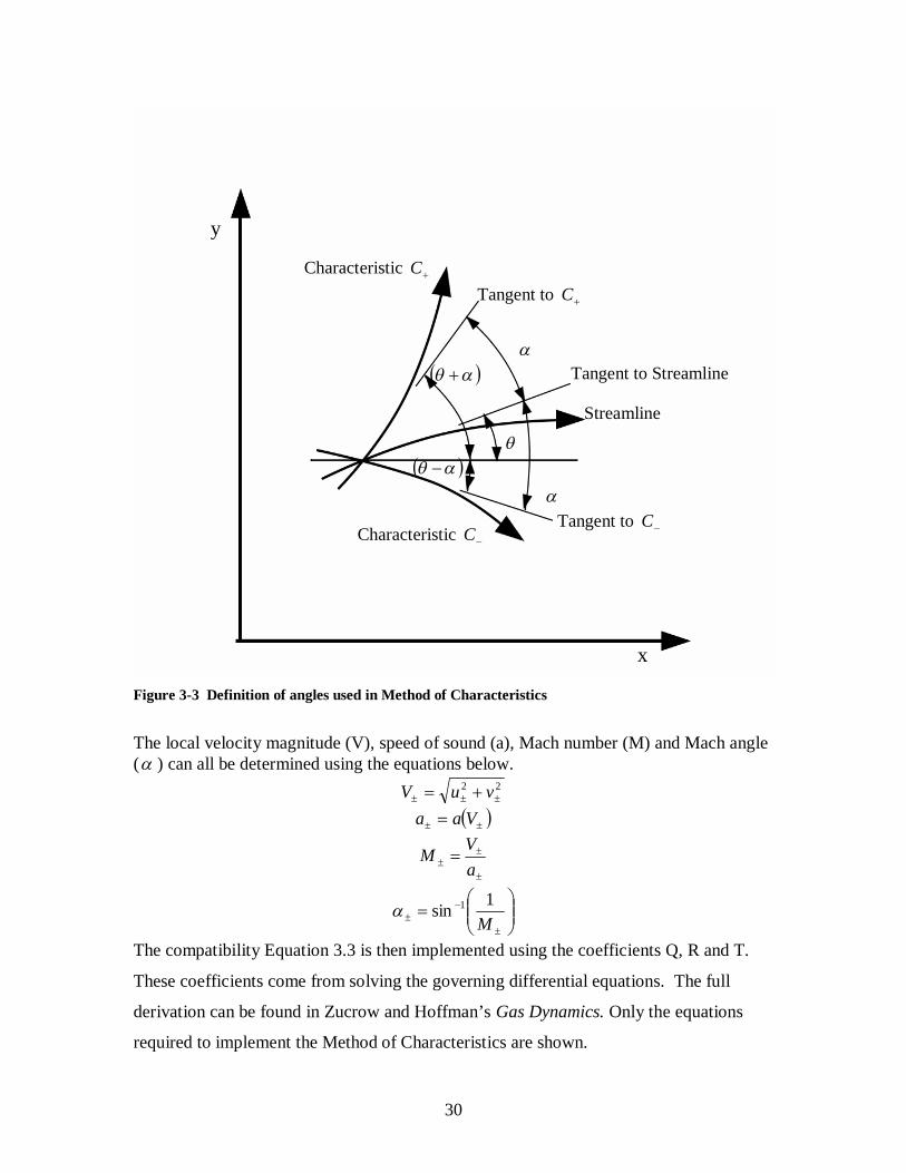
Figure 3-3 shows how the angles and are related to the characteristic lines and the

streamline. The local slope of the streamline of the flow ( ) is used to determine the

angle of the characteristic lines. The Mach angle ( ) represents the region of influence

of a point at a given Mach number. The triangle (or cone in three dimensions) formed by

the lines tangent to the C and C characteristic lines is the region of influence of the

point of known value, where the characteristics and streamline intersect. The known

point does not directly influence the properties of any point outside of this region of

influence.

30

Figure 3-3 Definition of angles used in Method of Characteristics

The local velocity magnitude (V), speed of sound (a), Mach number (M) and Mach angle ( ) can all be determined using the equations below.

22 vuV

Vaa

a

VM

M

1sin 1

The compatibility Equation 3.3 is then implemented using the coefficients Q, R and T.

These coefficients come from solving the governing differential equations. The full

derivation can be found in Zucrow and Hoffman’s Gas Dynamics. Only the equations

required to implement the Method of Characteristics are shown.

y

x

Characteristic C

Characteristic C Tangent to C

Tangent to C

Streamline

Tangent to Streamline

31

TvRuQ 44 Equation 3.3

where

22 vRuQT

11 vRuQT with

22 auQ

QvuR 2

A special case of an interior point is an axis of symmetry point. These occur along the

centerline of the primary plume. Figure 3-4 shows a typical axis point, where point 4, the

point of interest, is on the centerline.

Figure 3-4 Method of Characteristics unit process for a symmetry point25

x

y

Center Line

32

If point 1 is on a C characteristic line through point 4, then it has a mirror image, point

2, on the C characteristic. The symmetry point is then solved for using the interior

process with the additional known values for transverse location (y), transverse velocity

( v ) and flow angle ( ) in Equation 3.4. At this point, the location is on the centerline,

the x-axis, which has a transverse location of 0. The direction of flow is found from

point 1 and point 2 which have equal influence and are mirror images of each other about

the x-axis. Therefore, the transverse components of the velocity cancel and the flow is

horizontal, resulting in a transverse velocity of 0. With no transverse component of

velocity, the streamline is along the centerline. The angle between the centerline and the

flow is also 0.

0444 vy Equation 3.4

3.2.2 Method of Characteristics Direct Wall Point Calculation A direct wall point occurs where the flow comes in contact with the wall of the primary

nozzle. For this case the direction of the flow velocity must equal the local slope of the

nozzle wall. The wall point 4 is defined where the C characteristic from known interior

point 2 intersects the nozzle. A typical direct wall point is shown in Figure 3-5.

33

Figure 3-5 Method of Characteristics unit process for a wall point25

Due to the C characteristic emanating from a point which does not physically exist in

the flow field, point 1, only one compatibility equation can be used to determine the

location and properties of the wall point. However, the nozzle geometry offers the

remaining required relationships of the transverse location (y) of the point of interest in

Equation 3.5 and the flow direction ( ) in relation to the slope of the nozzle ( nozzle )

Equation 3.6. As shown in Figure 3-5 the point of interest with unknown properties lies

on the wall of the nozzle. Therefore, the transverse location of the point of interest can

be found once the stream wise location of the point is determined and input into the

function defining the nozzle wall geometry. Not only must the location of the wall point

conform to the nozzle geometry, the direction of flow of the wall points must also

conform to the slope of the nozzle wall, making the nozzle wall a streamline.

xyy nozzle4 Equation 3.5

x

y 1

34

nozzleuv

dxdy tantan

4

4 Equation 3.6

Using these equations as well as the familiar compatibility equations, Equation 3.1 and

Equation 3.7, the location (x and y) and properties at point 4 are determinable using a

similar process as the interior points. Recall Q, R and T are the coefficients found from

solving the governing differential equations. The tangent of the slope of the

C characteristic line emanating from point 2 is .



3.2.3 Method of Characteristics Free Pressure Boundary Point Calculation

The free pressure boundary point occurs on the boundary of the primary plume beyond

the end of the primary nozzle. The fundamental characteristic of this condition is that the

pressure on the boundary of the primary plume must match the pressure of the secondary

flow. Figure 3-6 shows the unit process for a free pressure boundary point.

35

Figure 3-6 Method of Characteristics unit process for free pressure boundary point

The secondary pressure is known, or assumed. The CPSE simulation begins with a guess

for the secondary pressure distribution. Once the primary plume has been solved for

using the Method of Characteristics, an updated secondary pressure distribution is

assumed. The total velocity magnitude (V) and static pressure (p) of the primary flow are

related by isentropic flow properties. The velocity at point 4, the location being solved

for, is given by Equation 3.8.

knownpfpfvuV s 421

24

244

Equation 3.8

The local stream-wise and transverse velocities (u and v) are related to the coefficients of

the finite difference equations, Q, R and T by Equation 3.7.


Free Pressure Boundary

Primary Nozzle Wall

C- Characteristic Curve

3

x

y 1

36

The simultaneous solutions of Equation 3.7 and Equation 3.8 yield formulations for the

stream-wise and transverse velocities at the point of interest. These formulations are

Equation 3.9 and Equation 3.10, respectively.

22

212222

44

RQ

TRQVRTQu Equation 3.9

212

42

44 uVv Equation 3.10

The final relationship required for the solution of a free pressure boundary point,

Equation 3.11, is the condition that the boundary of the primary plume is along a stream

line. The direction of flow (vu ), along line 3-4, must be equal to the slope of the plume

boundary, 0 .

0uv

dxdy

Equation 3.11

The relationship between the components of the streamline along the free pressure boundary is shown graphically in Figure 3-7 .

37

Figure 3-7 Components of the velocity vector along the free pressure boundary streamline

3.3 Secondary Stream Calculation Method The secondary stream of the ejector is analyzed using one-dimensional isentropic

relations. The secondary stream is divided into vertical slices. The isentropic relations

are evaluated at each slice. The distribution of the “slices” is determined by the free

pressure boundary points from the Method of Characteristics. This method of dividing

the secondary stream to correspond closely with the free pressure boundary points

reduces the amount of interpolating required by the Method of Characteristics algorithm

while it matches the pressure distribution of the primary and secondary streams along the

free pressure boundary.

The geometry of the primary plume determines the available flow area of the secondary

stream. The secondary stagnation conditions are related to the allowable flow area to

x

y

dyx

dxx

u

v

Tangent to Free Pressure Boundary Streamline

Free Pressure Boundary

38

determine the properties within the flow. Figure 3-8 shows the Mach number distribution

of the secondary flow using the isentropic area relations. The flow area of the secondary

plume is bounded on top by the ejector duct wall. The primary nozzle wall and the

primary plume serve as a lower bound of the secondary flow area. The secondary stream

is discretized into tall cells separated by thin black lines. The properties within each cell

are constant. The properties change only in the stream wise direction and are assumed

constant in the transverse direction.

Figure 3-8 The Mach number of secondary flow using isentropic area relations.

3.3.1 Mach number solution The Mach number distribution in the secondary flow is driven by the primary plume

geometry. The minimum area of allowable secondary flow occurs where the difference

between the area of the primary plume and the duct area ( DuctA ) is minimum. This occurs

where the primary plume area is at a maximum ( PlumeMaxA ). At the stream wise location

of the minimum secondary flow area, the secondary flow area is set to the critical

condition ( *SA ). This is shown in Equation 3.12.

PlumeMaxDuctS AAA * Equation 3.12

Secondary Flow

Primary Plume

Secondary Flow

Duct Wall

Nozzle Wall

DuctA PlumeMaxA

Mach Number

*SA

i = 1 2 3 . . . n . . . . . . . . . N

39

Using the known secondary area at each point in the streamwise direction ( SiA ) and

Mach number of unity at the critical point, the Mach number of the secondary flow at

each point in the streamwise direction ( SiM ) is found by solving Equation 3.13

iteratively23.

*

121

2

21

11

21

S

SiSi

Si AAM

M

Equation 3.13

The subscript i refers to the index used when discretizing the secondary stream into cells.

The indexing, like the discretization it describes is derived from the free pressure

boundary points found using the Method of Characteristics in the primary plume.

However, the indexing scheme is used to describe the entire secondary stream, including

the region before the mixing chamber. Therefore, the subscript 1 would be reserved for

the cell which begins at the secondary inlet and ends at the exit of the primary nozzle.

The properties in cell 1 are constant because the properties are determined using inviscid

calculations of the isentropic relations with no heat addition. Since there is no area

change, the Mach number and subsequent properties are constant in this area. The

designation of the cells continues sequentially with the secondary cell indicated by

subscript 2. When an arbitrary cell is being referred to the subscript i is used. Equation

3.13 uses the i subscript notation to indicate that the Mach number of any cell which can

be found using the available area of secondary flow into that same cell. From the area of

the cell face (the left hand side of any cell of interest in Figure 3-8) the Mach number is

found and assumed to be constant within the cell. The properties within the secondary

flow are solved for using the newly found Mach number distribution.

3.3.2 Isentropic values The secondary stagnation properties and the Mach number distribution determine the

properties in the secondary flow. The secondary stagnation temperature ( ST0 ), pressure

( SP0 ) and density ( S0 ) are known from the conditions from which the ejector is

entraining flow. Typically these properties are based on ambient conditions at the

40

entrance of the ejector. The secondary conditions may not be equal to the ambient or exit

conditions, for instance, if the secondary flow is entrained from a plenum.

Within each cell of the discretized secondary stream, the local static temperature ( SiT ),

pressure ( Sip ), and density ( Si ) is found using the Mach number of the cell of interest

of the secondary flow ( SiM ) and the isentropic Mach number relations shown in

Equation 3.14, Equation 3.15 and Equation 3.1623. The ratio of specific heats ( ) for the

fluid being entrained into the secondary flow is also required for these calculations.

2

0

211 Si

SSi

M

TT

Equation 3.14

12

0

211

Si

SSi

M

Pp Equation 3.15

12

0

211

Si

SSi

M

Equation 3.16

3.4 Iteration Scheme As previously stated, the primary and secondary streams drive the properties within the

other. The primary plume geometry is dependent on the pressure distribution of the

secondary stream. The pressure distribution of the secondary stream is dependant on the

geometry of the primary plume. In order to start the calculation process, an initial guess

of the pressure distribution of the secondary stream is made. This initial guess is then

41

refined through iterations of the primary plume geometry feeding into the secondary

stream properties and the secondary stream properties shaping the primary plume

geometry. Left unaltered, this iteration scheme is highly unstable and slow to converge

on a solution.

3.4.1 Relaxation Factors A relaxation factor is implemented to reduce fluctuations in the iteration scheme. The

relaxation factor works by incrementally changing the secondary pressure distribution

guess in the direction of the final solution. The secondary pressure distribution ( Sp ) to

be used for the Method of Characteristics in the next iteration is found as a weighted

combination of the newly found static pressure distribution ( SNewp ) and the pressure

distribution from the previous iteration ( SOldp ). The weighting is determined by the

relaxation factor (k) and shown in Equation 3.17. The value of the relaxation factor can

vary between 0 and 1. A fully relaxed case with relaxation factor of 1 will have no

update and never converge. Using a relaxation factor of 0 provides no relaxation factor.

The results jump violently from one iteration to the next and may become unstable or

never converge. A relaxation factor between 0.75 and 0.85 provides a fairly stable

convergence patterns and run times on the order of 90 seconds. Iteration count and run

times increase near the limits of aerodynamic flow patterns. For instance the iteration

count and run time of a case which borders on a blocked aerodynamic flow pattern and a

Fabri choke condition may take several minutes because the values of the intermediate

iterations jump between maximum secondary Mach numbers of 1 for the Fabri choke

condition and secondary Mach numbers of 0 for the blocked case.

SNewSOldS pkpkp 1 Equation 3.17

3.5 Entrainment Ratio Calculation The entrainment ratio of the ejector is the primary issue being investigated in this study.

Entrainment ratios and similar measurements have been discussed by Fabri, Addy,

Emanuel, Foster, Gist and others as a standard for ejector performance. The experimental

entrainment ratios found by Gist provide a benchmark with which to evaluate the

42

accuracy of the CPSE simulation. The entrainment ratio ( ) is the ratio of the mass flow

rate of the secondary stream ( sm ) relative to the mass flow rate of the primary stream

( pm ). The entrainment ratio shown in Equation 3.18 is a common measure of ejector

efficiency.

p

S

mm

Equation 3.18

As Equation 3.18 indicates, the mass flow rates of the secondary and primary streams

must be solved for in order to calculate the entrainment ratio. However, because the

ejector under investigation is two-dimensional and planar, the height of the ejector is

constant; therefore the height is not accounted for in the simulation. In reality, varying

the height (h) of the ejector would cause changes in performance due to fictional losses

on the ejector surfaces because a different portion of the flow would be affected by the

boundary layer. However, for a two-dimensional planar ejector with an inviscid analysis,

this height term will cancel out of the entrainment ratio equation without changing the

result; as is apparent in Equation 3.19.

hmhm

P

S

//

Equation 3.19

Although the terminology is not completely accurate, the values of mass flow rate

divided by height will still be referred to as mass flow rates.

The primary mass flow rate is found at the primary nozzle throat using the nozzle

geometry and the stagnation conditions. The critical area of the primary nozzle throat

( *PA ) is actually the width of the throat. As previously stated, the height of the ejector is

not considered. The chamber pressure of the primary stream ( PP0 ), the chamber

temperature of the primary stream ( PT0 ), the ratio of specific heats ( ) and gas constant

( R ) for the fluid of the primary plume are also required. Since the primary and

secondary flows are assumed to be similar in the CPSE simulation and experiments, the

43

gas constant and ratio of specific heats of the primary stream fluid are considered to be

the same as those of the secondary stream fluid. It is evident in Equation 3.20 that the

mass flow rate of the primary plume is not affected by any of the secondary flow

properties.

121

0

0*

12

P

PPp RT

PAm

Equation 3.20

The secondary mass flow rate is calculated at the point where the secondary stream

achieves a sonic condition. This occurs at the point of minimum secondary flow area.

This either occurs in the mixing chamber due to the expansion of the primary plume as in

the Fabri choke case, or it occurs in the entrance of the duct before being exposed to the

primary plume as in the saturated flow condition. The secondary mass flow rate ( Sm ) is

dependent on the geometry of the primary plume and the critical density ( *S ) and

velocity ( *SV ) within the flow as shown in Equation 3.21. The critical static pressure

( *Sp ), density, temperature ( *

ST ) and velocity were found using, Equation 3.22, Equation

3.23, Equation 3.24 and Equation 3.25 and the stagnation conditions of the secondary

flow. The ratio of specific heats and the gas constant of the secondary flow fluid are also

required.

***SSSS VAm Equation 3.21

1

0*

12

SS Pp

Equation 3.22

44

1

0*

211

S

S Equation 3.23

211

0*

S

STT

Equation 3.24

**SS RTV

Equation 3.25

This analysis is used for the saturated case and the Fabri choke condition. The exception

to this process is the trivial blocked case, there is no location of sonic condition in the

secondary flow and the mass flow rate is zero.

4 Results of the CPSE Simulation Unlike the one-dimensional, Fabri and Addy methods, this analysis is not concerned with

the flow properties beyond the point of minimum secondary flow area. The analysis is

only concerned with the region from the primary nozzle throat until the primary plume

achieves maximum expansion. Within these parameters, three cases are possible. The

three possible aerodynamic flow patterns are the saturated case, the supersonic case, also

termed Fabri choke, and the blocked case. The secondary stream becomes choked in the

saturated and Fabri choke conditions. The blocked case is unique in that the secondary

stream is not choked. The secondary flow velocity is zero in the blocked case.

All of the simulations are run using the geometry of the existing CPSE experimental test

rig. The primary and secondary streams are both composed of air with similar stagnation

temperatures. The height of the ejector is 0.75 inches. The primary nozzle has a throat

width of 0.1 inches and an exit width of 1.0 inches. The expansion ratio of the primary is

nozzle 10. The primary nozzle has a divergence angle of 15.35°. The lip of the nozzle

45

base is 0.25 inches thick. Each of the two secondary inlet ducts has a width of 0.625

inches. Within the mixing chamber the duct walls diverge at an angle of 3°. This 3°

divergence was implemented as a requirement for tests in which combustion occurs in the

mixing chamber. This divergence is not taken into account in the CPSE simulation and

does not exist in updated revisions of the CPSE test apparatus. A dimensioned top view

of the CPSE test apparatus is shown in Figure 4-1.

1.000 in

0.625 in

1.875 in

12.000 in

7.900 in

3.164 in

0.250 in

Divergence Angle 3.0°

Manifold Mixing Duct

Secondary Duct

Secondary Duct

Primary Ejector

11

Figure 4-1 Dimensioned top view of the CPSE test apparatus4

4.1 Saturated Supersonic Flow Pattern The lowest stagnation pressure ratios achievable with supersonic ejectors yield the

saturated aerodynamic flow pattern. The saturated case is characterized by secondary

flow achieving a critical Mach number before coming into contact with the primary

plume. This condition is caused by the relatively high secondary stagnation pressure

dominating the primary plume shape. For the CPSE configuration the saturated condition

will occur with pressure ratios below 73; although, this value is dependant on numerous

factors, especially geometry.

Figure 4-2 shows a CPSE simulation of the Mach number distribution of a saturated flow

pattern with a primary to secondary stagnation pressure ratio of 70. The large secondary

stream flow area and stagnation pressure allow the optimal amount of fluid to be

46

entrained by the supersonic primary plume. For this pressure ratio an entrainment ratio

of 0.18 is achieved.

Figure 4-2 CPSE simulation of the Mach number distribution of a saturated flow pattern

Figure 4-2 shows a truncated view of the Mach number distribution within the flow field.

First, only the top half of the flow field is shown because the flow is symmetric about the

centerline of the primary nozzle (the x axis). Also, once the primary plume has achieved

the maximum area, the Method of Characteristics calculations halt and the values are fed

forward for secondary stream calculations. Once the primary plume has achieved the

maximum area, the entrainment ratio can be determined. The properties of the flow field

beyond this point are not of interest to this investigation because finding the entrainment

ratio and the location where the secondary flow becomes sonic is the goal of the

calculation. It is important to note that the axes of the plot have also been skewed to

Primary Plume

Duct Wall

Primary Nozzle

Secondary Stream

Mach Number

47

provide a more detailed view of the flow phenomena occuring. The transverse direction

is enlarged compared to the streamwise direction.

The secondary flow is bounded on the upper surface by the duct wall. The primary

nozzle and the primary plume are the lower bound of the secondary plume. The

secondary stream achieves a critical Mach number in the inlet of the secondary stream

before coming into contact with the primary plume. The Mach number of the secondary

stream remains constant throughout the flow field.

The Mach number distribution in Figure 4-2 and the static pressure distribution in Figure

4-3 show many of the same trends. Both plots show that a large recirculation zone exists

in the area bounded by the primary nozzle, the primary plume and the secondary stream.

This recirculation zone is assumed to be pressure matched to the secondary stream and

the boundary of the primary plume. Since the Mach number in the secondary stream is

constant, the secondary pressure distribution is also constant. This requires the

recirculation zone to have a constant pressure as well. Both physically and in the CPSE

simulation, the recirculation zone is caused by the thickness of the nozzle lip. The nozzle

lip cannot be brought to a sharp point due to structural requirements. This recirculation

zone allows the primary plume boundary to gradually turn until it becomes parallel to the

secondary stream flow direction.

48

Figure 4-3 CPSE simulation of the static pressure distribution of a saturated flow pattern

Even with the gradual turning of the primary plume boundary facilitated by the

recirculation zone, a compression shock emanates from the nozzle lip due to the

interaction with the secondary stream. The secondary flow in the saturated case has

relatively high energy compared to the other aerodynamic flow patterns. The oblique

shock traces the peaks of the contour lines from the nozzle lip to the centerline of the

flow. This shock was also detected in experimental testing. This shock emanating from

the nozzle lip occurs to some extent in all the aerodynamic flow patterns. However, the

shock is the strongest in this case, determined by the angle it travels from the nozzle lip

and the effect on the Mach number and pressure beyond the shock. The strength of the

shock causes a discontinuity in the properties of the flow which is not handled well by the

MOC scheme. The MOC scheme smears this change of properties though a finite area.

Duct Wall

Primary Nozzle

Secondary Stream

Static Pressure [lb/sqft]

Primary Plume

49

Some nodes downstream of the shock appear to be small regions of increased Mach

number or decreased pressure. This phenomenon is numerical and not physical.

For this saturated condition, the secondary flow becomes choked before coming into

contact with the primary plume. The primary plume is allowed to expand in the mixing

chamber due to the recirculation zone caused by the thickness of the primary nozzle lip.

The primary plume achieves maximum expansion 4 inches beyond the throat of the

primary nozzle for the given geometry and a pressure ratio of 70.

4.2 Fabri Choke Supersonic Flow Pattern The supersonic Fabri choke condition is characterized by the secondary flow achieving a

critical Mach number due to expansion of the primary plume. The secondary flow

chokes in the mixing chamber where the primary plume achieves its maximum area.

This aerodynamic flow pattern occurs when the primary to secondary stagnation pressure

ratio is too high to result in the saturated case and too low to block the secondary flow.

Typical pressure ratios for this condition with the CPSE configuration range between 73

and 230, this range of pressure ratios will vary with numerous factors, especially ejector

geometry.

Figure 4-4 shows a CPSE simulation of the Mach number distribution of a Fabri choke

supersonic flow pattern. This case was run with a primary to secondary stagnation

pressure ratio of 125. The ratio of secondary to primary mass flow rates is 0.073.

50

Figure 4-4 CPSE simulation of the Mach number distribution of a Fabri choke supersonic flow pattern

The incoming secondary stream is subsonic with a Mach number near 0.5. The

secondary flow is accelerated by the primary plume until it reaches the critical velocity at

the point of minimum secondary flow area. The primary to secondary stagnation

pressure ratio is higher than the saturated case, enabling the primary plume to expand,

reducing the secondary flow area.

Both Figure 4-4 and the static pressure distribution in Figure 4-5 show that the Fabri

choke supersonic case also shows the compression shock in the primary plume emanating

from the lip of the primary nozzle. The shock hinders the acceleration of the primary

plume as the plume expands into the secondary flow area.

As in the saturated case, there is a recirculation zone beyond the lip of the nozzle. The

recirculation zone occurring in Fabri choke conditions is much smaller than that of the

Duct Wall

Primary Nozzle

Secondary Stream

Primary Plume

Mach Number

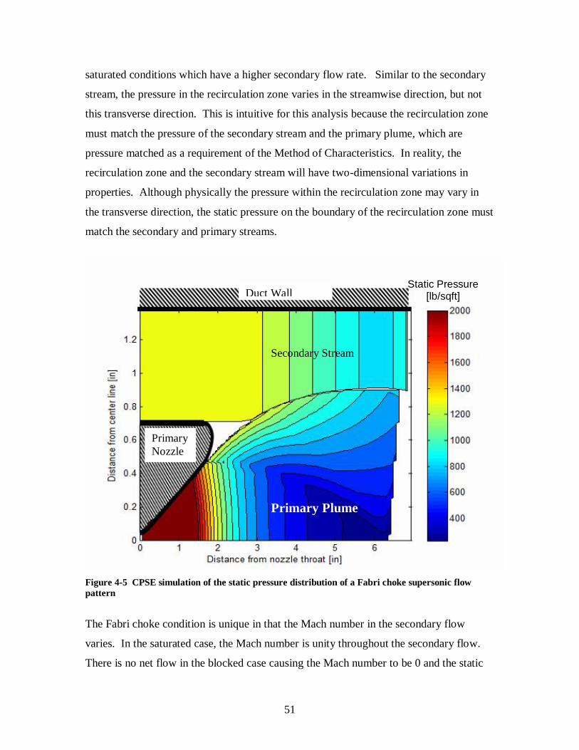
51

saturated conditions which have a higher secondary flow rate. Similar to the secondary

stream, the pressure in the recirculation zone varies in the streamwise direction, but not

this transverse direction. This is intuitive for this analysis because the recirculation zone

must match the pressure of the secondary stream and the primary plume, which are

pressure matched as a requirement of the Method of Characteristics. In reality, the

recirculation zone and the secondary stream will have two-dimensional variations in

properties. Although physically the pressure within the recirculation zone may vary in

the transverse direction, the static pressure on the boundary of the recirculation zone must

match the secondary and primary streams.

Figure 4-5 CPSE simulation of the static pressure distribution of a Fabri choke supersonic flow pattern

The Fabri choke condition is unique in that the Mach number in the secondary flow

varies. In the saturated case, the Mach number is unity throughout the secondary flow.

There is no net flow in the blocked case causing the Mach number to be 0 and the static

Duct Wall

Primary Nozzle

Secondary Stream

Primary Plume


52

pressure to be the stagnation pressure. However, the plume in the Fabri choke case must

match the continuously variable pressure distribution of the secondary stream. The

continuous pressure matching of the streams is displayed in Figure 4-5.

For this trial, the primary plume achieves maximum expansion nearly 6 inches beyond

the exit plane of the primary nozzle in the stream wise direction. This location of

maximum plume expansion is significantly further down stream than that of the saturated

condition. Note the change in scale when comparing the saturated case to the Fabri

choke cases.

4.3 Blocked Flow Pattern The blocked case is characterized by a primary plume which comes in contact with the

duct walls, blocking off the secondary flow. The primary to secondary stagnation

pressure ratio must be very high to achieve a blocked condition. Although it is heavily

dependent on geometry, for the CPSE geometry, the blocked case will generally occur

above pressure ratios near 230. Figure 4-6 is a CPSE simulation of the Mach number

distribution of a blocked flow pattern. The primary to secondary stagnation pressure ratio

for this case is 250. There is no secondary flow entrained.

53

Figure 4-6 CPSE simulation of the Mach number distribution of a blocked flow pattern

The large primary to secondary stagnation pressure ratio facilitates rapid expansion of the

primary plume. The primary plume expands all the way to the duct wall. The secondary

flow is completely blocked. The incoming secondary flow rate is zero. Although there

may be some recirculation in this area, the net mass flow of the secondary flow is zero.

The low secondary stagnation pressure results in the least amount of flow turning of the

primary plume. This reduced influence on the primary plume induces the weakest

compression off the primary nozzle lip. The high primary chamber pressure also results

in the highest primary Mach number.

Figure 4-7 shows the static pressure distribution of the blocked flow pattern. Similar to

the saturated case, the static pressure in the secondary stream is constant. For this

condition, the secondary static pressure is the stagnation pressure from which the air is

being entrained. This constant pressure in the secondary stream means that the primary

plume boundary is also constant in pressure.

Duct Wall

Primary Nozzle

Secondary Stream

Primary Plume

Mach Number

54

Figure 4-7 CPSE simulation of the static pressure distribution of a blocked flow pattern

The primary plume intersects the duct wall approximately 6.5 inches from the primary

nozzle in the streamwise direction. This streamwise location of maximum primary plume

expansion is comparable to that of the Fabri choke case. However, this maximum plume

expansion location is definitively further downstream than both the Fabri choke and the

saturated aerodynamic flow patterns. However, it cannot be assumed that the maximum

expansion of the blocked case will always be the largest. At a pressure ratio of 262, the

primary plume intersects the duct wall less than 5.5 inches downstream of the primary

nozzle throat. Once the aerodynamic flow pattern reaches a blocked case, increasing the

pressure ratio will decrease the distance where the primary plume achieves maximum

expansion. This phenomenon is easily explained. The primary plume expands at a

steeper angle when the secondary stagnation pressure is lower. This more rapid

expansion of the primary plume causes the plume to intersect the duct wall at a location

Duct Wall

Primary Nozzle

Secondary Stream

Primary Plume


55

further upstream than cases of lower pressure ratios where the secondary stream hinders

the expansion of the primary plume.

5 Comparisons to Previous Work In order to evaluate the quality of the results from the CPSE computer simulation,

previous work is used as a standard. The experimental and theoretical investigations of

Gist provide a database with which to measure accuracy. The one-dimensional methods

used by Gist and Foster to approximate the flow field properties within the ejector do not

provide high fidelity illustration of the flow interactions. However, Gist and Foster both

made attempts to characterize the geometry of the primary plume. Flow visualization and

entrainment ratio observations from these previous studies are used to validate the

accuracy of the CPSE simulation.

The most readily verifiable hypothesis posed on the geometry of the flow field was

Foster’s proposal that the streamwise location of maximum primary plume expansion is

unchanged by pressure ratio. The results from the CPSE simulation clearly show that as

pressure ratio is increased, the location of maximum plume expansion moves downstream

until the blocked flow pattern exists. Once the blocked flow pattern occurs, the point

where the primary stream reaches maximum expansion begins to move back upstream.

The CPSE simulation produced data which adds fidelity to the hypothesis of Foster. The

flow visualization results interpreted by Foster and Gist produce this result within the

accuracy capability of the flow visualization technique. Figure 5-1 and Figure 5-2 show

the visualizations of Gist and Foster in which the streamwise direction measurement

starts at the primary nozzle lip while the CPSE simulation takes the primary nozzle throat

to be the starting point of the measurement.

56

Figure 5-1 Nitrogen condensation plume in the mixing chamber at a pressure ratio of 954

Figure 5-2 Methane and Oxygen thruster fired at a pressure ratio of 2010

Gist estimated the shock structure within the primary plume based on the condensation

patterns in the photographic flow visualization of his experiments. Figure 5-3 shows the

condensation shock structure recorded by Gist as well as Gist’s superimposed shock

structure. The image displays the expansion and compression cycle emanating from the

lip of the nozzle. The onset of this shock cycle is also present in all aerodynamic flow

patterns calculated by the CPSE simulation and shows the expected increase in size as the

pressure ratio increases.

57

Figure 5-3 Video frame and superimposed shock structure from cold flow tests4

In addition to showing the start of expansion compression cycles, the CPSE simulation results also match CFD studies which have been conducted on the recirculation zones near the nozzle lip of supersonic ejectors 30. Figure 5-4 shows the work of Purdue researchers Gujarathi, Li, Anderson and Sankaran. The low secondary flow rate represents a case of higher pressure ratio than the case of high secondary flow rate. The observations of the simulation results section above indicate that as the secondary flow decreased from saturated to Fabri choke to blocked cases, the size of the recirculation zone shrinks. Figure 5-4 reaffirms that larger secondary flow rates result in larger recirculation zones.

58

Nozzle Base

Nozzle Base

Low Secondary Flow Rate

High Secondary Flow Rate

Figure 5-4 Mach Number and Streamlines from CFD Model30

The visual data acquired from the Gist and Purdue studies affirm that the CPSE

simulation is capturing the correction trends in flow interactions. However, in order to

numerically assess the accuracy of the CPSE simulation quantitative data such as

entrainment ratios must be compared. Gist conducted a theoretical and experimental

investigation of the influence of pressure ratio on entrainment ratio. Figure 5-5 shows the

theoretical entrainment ratio distribution estimated by Gist. The saturated calculation

presented previously in Equation 2.1 is used as a baseline to estimate the entrainment

ratio, the ratio of secondary to primary mass flow rates. Gist then applies the empirical

correction factor for primary plume growth represented by the different andK exp values.

The andK exp value of 1.0 represents ideal expansion of the primary plume with a

correction for the thickness of the primary nozzle lip. The primary to secondary

stagnation pressure ratio near 72 is the optimal expansion condition.

59

0.06

0.08

0.10

0.12

0.14

0.16

0.18

0.20

0.22

0.24

0.26

0.28

0.30

0.32

40 50 60 70 80 90 100 110 120

Total Pressure Ratio

Ent

rain

men

t Rat

io (Φ

)

Kexpand = 1.0Kexpand = 1.5Kexpand = 2.0Saturated Case

OPT

IMA

L E

XPA

NS

ION

Fabri Mode

Figure 5-5 Entrainment ratio calculations using empirical correction factor for plume size4

As the location of the optimal expansion suggests, higher entrainment ratios do not

indicate better performance. Optimal performance occurs at the pressure ratio where the

mass flow rate is maximum for the given ejector. Pressure ratios above the optimal

condition result in a primary plume which expands into the secondary flow area. This

reduced area of the secondary flow results in a decreased secondary mass flow rate.

Pressure ratios below optimal conditions result in a saturated flow pattern with a higher

entrainment ratio. This condition is suboptimal because the primary plume is not

providing the maximum mass flow. Although the Mach number of the primary flow is

dictated by the nozzle geometry, the mass flow of the primary plume is a function of the

chamber pressure. The pressure ratio of optimal plume expansion yields the maximum

mass flow of both the primary and secondary streams.

60

Gist’s empirical correction factors are only implemented at pressure ratios above that

which yield optimal expansion. The empirical correction factors do not alter the

entrainment ratio at pressure ratios below optimal expansion because the primary plume

does not expand into the secondary flow area when operating in the saturated flow

regime.

Figure 5-6 shows the lines of the theoretical approximations of Gist with the

corresponding experimental results represented by blue asterisks. The experimental data

points show some fluctuation, however, they correspond closely to a andK exp value of 1.5.

The approximation of Gist is able to closely predict the experimental data when the

correction factor is implemented. However, a large amount of empirical knowledge is

required to perform such an analysis. The proper andK exp value for a specific geometry

must be determined experimentally and the point of optimal expansion must also be

known. An incorrect estimation of andK exp can result in errors of over 20%.

61

Figure 5-6 Comparison of CPSE computer code to experimental data and empirical predictions

Figure 5-6 also shows that Gist’s experimental and theoretical results provide excellent

validation for the numerical CPSE computer simulation. The red circles in the plot are

data points from the CPSE computer simulation which very closely follow the trend of

the data throughout the range of pressure ratios, despite fluctuations in the experimental

data. The CPSE simulation does not implement any empirical correction factors or

require any apriori knowledge to achieve this level of accuracy. The only parameters

required by the CPSE simulation are the geometry of the ejector and the stagnation

conditions of the primary and secondary streams. The average error between the CPSE

numerical simulation and the experimental data is 3.67%. In every case the CPSE code

slightly under predicted the entrainment ratio. Some of this under prediction is likely due

to the 3° divergence in the duct walls of the CPSE experimental apparatus which is not in

the CPSE simulation. However, it is estimated that by running more pressure ratios

experimentally and in the simulation, the average error would be reduced without

modification of the simulation. The noise in the experimental data suggests some

CPSE Code

62

unsteady operation of the ejector occurred. Gist suggests leakage and asymmetrical

entrainment take place in some of the trials. More trials at each pressure ratio will

provide experimental results with less noise that can be better used to evaluate the

accuracy of the CPSE simulation. The future versions of the CPSE test apparatus will

not have diverging duct walls which will aid in isolating likely the cause of the error.

Some deviation may also occur due to the inviscid method of analysis used by the CPSE

simulation. It is of interest to quantify the influence of viscous effects on the entrainment

ratio.

6 Conclusions The CPSE computer code is an automated simulation of the two-dimensional planar Cal

Poly Supersonic Ejector. The application of the most relevance for this simulation is a

rocket based combined cycle hypersonic propulsion system operating in the air

augmented rocket mode for takeoff and acceleration in the subsonic flight regime. Hot

fire combustion tests were conducted with the CPSE at low pressure ratios. Cold flow

tests were run with higher pressure ratios. Both sets of tests entrained air from ambient

conditions. The experiments with the higher pressure ratios were approximated by

equations based on Fabri’s quasi-one-dimensional method with an empirical correction

factor added to increase accuracy. The CPSE simulation is a higher fidelity numerical

approximation method without the need for empirical correction factors or apriori

knowledge of the flow phenomena in the various aerodynamic flow patterns. The CPSE

simulation was developed using the work of Addy as a foundation. The Method of

Characteristics is used to describe the primary plume of the supersonic ejector with an

initial guess for the pressure distribution of the secondary flow. The secondary flow

properties and updated pressure distribution are solved using isentropic relations and the

geometry of the primary plume determined by the Method of Characteristics. The

pressure distribution of the secondary flow is fed back into the Method of Characteristics

and this process iterates until the solution of the primary and secondary streams

converges.

63

The Method of Characteristics provides the properties and geometry of the primary

plume. These properties vary in the streamwise and transverse direction. The secondary

stream is solved using isentropic relations and only varies in the streamwise direction.

There are no viscous or thermo-chemical reactions taken into consideration in the

simulation.

Saturated, supersonic Fabri choke and blocked aerodynamic flow patterns were seen in

the CPSE simulation as the primary to secondary stagnation pressure ratio is increased.

As the pressure ratio is increased, the entrainment ratio decreases. Optimal expansion

occurs at the transition from the saturated case to the Fabri choke condition. During

optimal expansion the ejector is operating most efficiently. The identification of the

optimal expansion pressure ratio of 74 agrees with experimental data from Gist and

Foster.

The presence of a weak shock in the primary plume emanating from the nozzle lip and a

recirculation zone at the nozzle lip were detected in all aerodynamic flow patterns. The

presence of the shock structure and recirculation zone at the nozzle lip is confirmed by

previous experiments. The simulation suggests that as pressure ratio is increased, the

compression shock decreases in strength and the recirculation zone shrinks in size. Both

these phenomena are due to the primary plume boundary being able to expand more

freely when the secondary stagnation pressure is lower. This trend of expansion causes

the location of maximum primary plume expansion to move downstream as the pressure

ratio is increased until the blocked case occurs. Once the blocked case occurs near a

pressure ratio of 230, the location of maximum primary plume expansion is dictated by

the primary plume’s intersection with the duct wall. Increasing the pressure ratio under

this condition causes the streamwise location of the primary plume’s intersection with the

duct wall to move upstream. This unhindered expansion of the primary plume would not

only decrease performance of air augmented ejector engines, but may also cause damage.

Using the Method of Characteristics for the primary supersonic plume and isentropic area

relations for the secondary plume, the CPSE computer simulation is able to accurately

64

predict entrainment ratios of supersonic air to air planar ejectors within 4%. The

accuracy of the simulation which has no viscous considerations suggests that ejectors

operating with a high supersonic primary plume have flow phenomena which are

governed by pressure distribution, not viscous effects. This rapid simulation algorithm

can be implemented for preliminary design analysis and determining which cases should

be examined using CFD and high fidelity methods. This simulation has already provided

insight for modification of the CPSE experimental test rig. The CPSE simulation results

have provided the required data for inlet sizing, plenum specifications and pressure

transducer location of the next CPSE experimental test rig.

7 Future Work Beyond the results presented within this paper, the CPSE computer simulation currently

has parametric capability yet to be validated. Geometry changes such as nozzle curvature

and dimensions, duct width, and duct wall contours are accepted by the simulation. Gas

composition can be modified by changing the ratio of specific heats of the fluids. The

stagnation temperatures of the gases may also be changed, although there are currently no

heat transfer considerations implemented in the simulation.

The CPSE computer simulation is coded in a manner which readily accepts additional

capability and fidelity. Several additions to the code are suggested. Viscous interactions

between the secondary flow and the duct walls should be implemented to determine the

effect of viscosity at different primary Mach numbers and primary to secondary

stagnation pressure ratios. Viscous effects between the primary plume and the secondary

flow should also be added to the capability of the CPSE simulation. These additions will

make the secondary stream analysis into a full two-dimensional method which will

provide much more realistic simulations of the flow phenomena occurring within the

ejector. Thermal and chemical interactions would allow the CPSE code to better

approximate the operation of an air augmented rocket operating with a fuel rich primary

plume. Simulations of flows with a hot primary plume can be validated using the

experimental results of Foster. However, these additions will increase computational

time. A more efficient iteration scheme would reduce run time and benefit parametric or

higher fidelity analyses.

65

The parametric capability of the CPSE simulation already built into the code can be taken

advantage of with more experimental data. The simulation cannot be used to its full

capacity without a test apparatus which can vary geometry and expand the regime of

pressure ratios. A variable geometry nozzle and movable duct walls would provide

validation for various ejector geometries within the two-dimensional planar category.

After an investigation is performed, the primary nozzle contour should be optimized for

performance. The current primary nozzle contour is designed for ease of manufacturing.

Furthermore, the addition of a low pressure plenum to the secondary flow inlet would

dramatically increase the range of experimentally examinable pressure ratios.

8 References 1. Lear, W.E., Sherif, S.A., Parker, G.M., “Effects of Fabri Choking on the

Performance of Two-Phase Jet Pumps”, AIAA 3012, January 2000. 2. Fung Sang Kang, Andrew, “Modeling of Mixer-Ejector Nozzle Flows”

Massachusetts Institute of Technology. February 1995. 3. Cutler, A.D., Magnotti, G., “Supersonic Combusting Jet Experiments for Code

Development and Validation” Defense Test Resource Management Center, Hypersonic Test Focus Area, NASA Fundamental Aeronautics Hypersonics Program.

4. Gist, Ryan, “Examination of Flow Field Characteristics and Fabri-Choking of a 2-D Air Augmented Rocket” California Polytechnic State University, January 2007.

5. Curry, Marty, “NASA Dryden Hyper-X/X43-A Graphics Collection”, http://www.dfrc.nasa.gov/Gallery/Graphics/Hyper-X/Large/X-43A_3view-color.jpg [retrieved April 3 2010].

6. Federation of American Scientists, “X-43 Hyper X Program”, http://www.fas.org/programs/ssp/man/uswpns/air/xplanes/x43.html [retrieved April 3 2010].

7. Curry, Marty, “NASA Dryden SR-71 Graphics Collection”, http://www.dfrc.nasa.gov/Gallery/graphics/SR-71/index.html [retrieved April 3 2010].

8. Warwick, Graham, “DARPA Cancels Hypersonic Blackswift”, Aviation Week [online], October 13, 2008. http://www.aviationweek.com/aw/generic/story.jsp?id=news/BLACK101308.xml&headline=DARPA%20Cancels%20Hypersonic%20Blackswift&channel=defense [retrieved April 7 2010].

9. Albertson, Cindy W., Emami, Saied, Trexler, Carl A., “Mach 4 Test Results of a Dual-Flowpath, Turbine Based Combined Cycle Inlet”, NASA Langley Research Center, Hampton, Va.

10. Foster, Trevor James, “Rectangular Ducted Methane/GOX Thruster”, February 2008. California Polytechnic State University.

66

11. Papamoschou, D., “Analysis of Partially Mixed Supersonic Ejectors”, Journal of Propulsion and Power, Vol. 12, No. 4, July 1996.

12. Fabri, J., and Siestrunk, Supersonic Air Ejectors”, Advances in Applied Mechanics, Vol. 5, Von Karman and Dryden, editors, Academic Press, 1958, pg 1-35.

13. Fabri, J., & Paulon, J., “Theory and Experiments on Supersonic Air-to-Air Ejectors”, NACA TM 1410, Sept 1956.

14. Addy, L.A., “On the Steady State and Transient Operating Characteristics of Long Cylindrical Shroud Supersonic Ejectors”, University of Illinios, Ph. D. dissertation. University Microfilms, Inc. Ann Arbor, MI., 1963.

15. Hall, J.L., Dimotakis,P.E., and Rosemann, H., “Experiments in Non-Reacting Compressible Shear Layers, AIAA-1991-0629, 29th Aerospace Sciences Meeting, Reno, 1991.

16. Grosche, C.E., Seiner,J.M.,Hussaini, M.Y., Jackson,T.L., “Numerical Simulation of Mixing Enhancement in a Hot Supersonic Jet.”

17. Seider, Warren D., Churchill, Stuart W., “Confined Jet Mixing in the Entrance of a Tubular Reactor”, AlChE Journal, University of Michigan, May 1971.

18. Emanuel, N.G., “Comparison of One-Dimensional Solutions with Fabri Theory for Ejectors”, Acta Mechanica 44, pgs. 187-200, 1982.

19. Huang, B.J., Chang, J.M., Wang, C.P., Petrenko, V.A., “A 1-D analysis of ejector performance”, International Journal of Refrigeration 22 (1999) 354-364. Department of Mechanical Engineering, National Taiwan University.

20. Mickelson, C.D, Sandberg , M.R, Addy, A.L, “Theoretical and Experimental Analysis of the Constant Area Supersonic-Supersonic MixerEjector”, October 1976.

21. Cutler, A.D., Carty, A.A., Doerner, S.E., Diskin, G.S., and Drummond J.P., “Supersonic Coaxial Jet Experiment for CFD Code Validation”, AIAA-99-3588, 30th AIAA Fluid Dynamics Conference, Norfolk, 1999.

22. Simonson, A.J., Schmeer, J.W., “Static Thrust Augmentation of a Rocket-Ejector System with a Heated Supersonic Primary Jet”, NASA TN D-1261, May 1962.

23. Zucrow, Maurice J., Hoffman, Joe D., Gas Dynamics Volume I. 1976. John Wiley and Sons, Inc. New York

24. Zucrow, Maurice J., Hoffman, Joe D., Gas Dynamics Volume II: Multidimensional Flows. 1977. John Wiley and Sons, Inc. New York

25. Riley, Paul. “Axisymmetric Method of Characteristics: An Algorithm and Its Validation”, California Polytechnic State University, June 13, 2008

26. De Chant, L.J. & Canton, J.A., “Measurement of Confined Supersonic, 2-D Jet-Lengths Using the Hydraulic Analogy”, Experiments in Fluids, Vol. 24, pgs. 58-65, Springer-Verlag, 1998.

27. Kouchi, T., Kobayashi, K., Murakami, A., Kato, K., Tomioka, S., “Performance of a RBCC Combustor Operating in Ramjet Mode”, AIAA 2006—4867, 42nd AIAA Joint Propulsion Conference, Sacramento, 2006.

28. Kobayashi, K., Tomioka, S., Kato, K., Murakami, A., and Kudo, K., “Performance of a Dual-Mode Combustor with Multistaged Fuel Injection”, Journal of Propulsion and Power, Vol. 22, No. 3, 2006.

67

29. Dimotakis, P.E., “Turbulent Free Shear Layer Mixing and Combustion” in Murthy, S.N.B., Curran, E.T., editors, High-Speed Flight Propulsion Systems, Progress in Astronautics and Aeronautics, Volume 137, pgs 265-340.

30. Batt, R.G., “Turbulent Mixing of Passive and Chemically Reacting Species in a Low-Speed Shear Layer”, Journal of Fluid Mechanics, Vol. 82, pp 53-95, Aug 1977.

31. Gujarathi, A., Li, D., Anderson, W., & Sankaran, V. “CFD Modeling of a Ducted Rocket Combined with a Fuel-Rich Primary Thruster”, 42nd Joint Propulsion Conference. AIAA 4577, July 2006

68

9 Appendix %Cal Poly Air Augmented Rocket Code %formulated and Coded by Brett Morham %January 14,2009 % %Method Of Characteristics provided by Paul Riley clc close all clear format compact tic %%%Notes%%%%%%%%%%%%%%%%%%%%%%%%%%%% %%%Fabriblock at PR>230%%%%%%%%%%%%% %%%Saturated at PR<70 (code will err below 30 due to imaginary velocities w/in iteration scheme) %%%%%Input Geometric properties of the ejector%%%% %%%%Nozzle Geometry & Thermodynamic Properties%%%%%%%%% theta_max = 15.35;%15.35; %max turning angle (degrees) theta_exit = 15.35; %theta_exit = 15.35; %wall angle at the nozzle exit (degrees) r_th= .05/12; %r_th= .05/12; %throat radius (ft) zlen = 1.65/12; %zlen = 0.3417; %nozzle length (ft) P0p = 1750*144;%1690*144 ;%P0p = 1350*144;% %trevor used 1032 psi%chamber stagnation pressure (psf) T0p = 521.7;%2000+475; %chamber stagnation temperature (deg R) roc_u = .22;%.1; (ft) radius_of_curvature_upstream roc_d = .1;%.10; %roc_d = 0.090695; %(ft) radius_of_curvature_downstream gamma= 1.4;%1.24; %ratio of specific heats for the working fluid R = 1774.864;%%gas constant for the primary flow (ft-lbf/slug R) delta = 0; %0 for planar, 1 for axisymmetric zduct = 14/12; %7.9 inches from nozzle lip %duct length [feet] from exit of nozzle. rduct = 2.75*0.5/12; %half duct width [ft] %this need to become a function tb = 0.25/12; %thickness of nozzle lip [ft] thetaduct = 0; %angle of wall divergence in degrees. if wall converges use negative angle Ta = 528.7; %stagnation temperature of secondary flow[Rankine] rhoa = .002102;%stagnation density of seconday flow [slug/ft^3] gammaa = 1.4; %ratio of specific heats of secondary flow. Rs = 1716; %Gas constant for secondary flow [ft2/s2*R] A_inlet = 6/12; %area of secondary inlet (must divide by duct height) [in] Pa = 6*144; %stagnation pressure of secondary flow [psf] %%%%Grid Size%%%%%

69

JMAX = 20; %JMAX = 161; %number of points in the j-direction IMAX = 1400;%IMAX=1400; intfigs = 0; %do you want to display graphs for each iteration? if so set to 1 %%Set initial guess values to start code %Ps = [Pa,Pa*0.53]; %initialize secondary flow if P0p/Pa >= 70 Ps = [Pa,0]; else Ps = [Pa/2,0]; end Zs = [zlen,zduct]; Ps_old = 0; guess = 1; update = 1; while update >= .5 [Zp,Rp,Rl,z,r,Mp,Pp,i_end,z_tr,coeff, mdotp] = AXImocFn(theta_max, theta_exit, r_th, zlen, P0p, T0p, roc_u, roc_d, gamma, R, JMAX, IMAX, delta,zduct,rduct,thetaduct,Ps,Zs); Ps_old = Ps; Zs_old = Zs; %%%%inputs%%%% if intfigs ==1 %% Use Interp to plot nozzle properties without characteristic lines xo = linspace (0,max(max(z)),500); %xo = linspace (0,z(1,i_end),50); yo = linspace (0,max(max(r)),500);%yo = linspace (0,r(JMAX,i_end),50); [x,y] = meshgrid(xo,yo); MI = griddata (z(:,1:i_end),r(:,1:i_end),Mp,x,y,'cubic'); %PI = griddata (z(:,1:i_end),r(:,1:i_end),Pp,x,y,'cubic'); figure surf (12*x,12*y,MI) %surf (12*x,12*y,PI) axis ([0,zduct*12*1.1,0,12*(rduct+tand(thetaduct)*zduct)]) % axis ([0,z(1,i_end)*12,0,12*(rduct+tand(thetaduct)*zduct)]) title ('Interpolated Mach Number Contours') %title ('Interpolated Pressure Level Contours') view(2) colorbar else end %% [Ms Ps Zs mdots Zd Rd Pd Md Ats] = SSFLOW2(Zp,Rp,zlen,Rl,rduct,thetaduct,gammaa,Pa,Ta,Rs,rhoa,intfigs,tb); update = max(abs(norm(Ps)-norm(Ps_old))) k = 0.8; % relaxation factor for iteration update. 0 for no relaxation. 1 for no update. crank up for steadier slower convergence.

70

Ps_old = interp1(Zs_old,Ps_old,Zs,'spline','extrap'); Ps = k*Ps_old+(1-k)*Ps; Ms; guess = 0; end Ms PR = P0p/Pa beta = 2*mdots/mdotp %% produce plots %%% %%% meshplot %%% res = 50; %resolution xo = linspace (0,max(max(z)),res); yo = linspace (0,max(max(r)),res); [x,y] = meshgrid(xo,yo); MI = griddata (z(:,1:i_end),r(:,1:i_end),Mp,x,y,'linear'); %PI = griddata (z(:,1:i_end),r(:,1:i_end),Pp,x,y,'cubic'); figure surf (12*x,12*y,MI) %contourf (12*x,12*y,MI,20) %surf (12*x,12*y,PI) axis ([0,12.2*max(Zp),0,12*(rduct+tand(thetaduct)*zduct)]) % axis ([0,z(1,i_end)*12,0,12*(rduct+tand(thetaduct)*zduct)]) title ('Interpolated Mach Number Contours') %title ('Interpolated Pressure Level Contours') xlabel ('Distance from nozzle throat [in]') ylabel ('Distance from center line [in]') view(2) colorbar hold on surf(12*Zd,12*Rd,Md) %contourf (12*Zd,12*Rd,Md,10) view(2) z_test =linspace(0,z_tr,100)'; plot(12*z_test,12*(-sqrt(roc_d^2-z_test.^2)+r_th+roc_d),'LineWidth',3,'Color','k') %plot the expansion section's circular arc z_test2 = linspace(z_tr,zlen,100)'; plot(12*z_test2,12*(coeff(1)+coeff(2).*z_test2+coeff(3).*z_test2.^2),'LineWidth',3,'Color','k') %plot the straightening section's parabolic contour rnoz = 12*(coeff(1)+coeff(2).*max(z_test2)+coeff(3).*max(z_test2.^2)); plot(12*[0,zlen],[rnoz+12*tb,rnoz+12*tb],'LineWidth',3,'Color','k') %plot the casing of the nozzle hold off %%%Characteristic plot%%% figure

71

hold on surf(12*z(:,1:i_end),12*r(:,1:i_end),Mp) title('Mach contours') view(2) colorbar z_test =linspace(0,z_tr,100)'; plot(12*z_test,12*(-sqrt(roc_d^2-z_test.^2)+r_th+roc_d),'LineWidth',3,'Color','g') %plot the expansion section's circular arc z_test2 = linspace(z_tr,zlen,100)'; plot(12*z_test2,12*(coeff(1)+coeff(2).*z_test2+coeff(3).*z_test2.^2),'LineWidth',3,'Color','g') %plot the straightening section's parabolic contour hold off %% toc function [Zp,Rp,Rl,z,r,M,P,i_end,z_tr,coeffs,mdot] = AXImocFn(theta_max,theta_exit,r_th,zlen,P0,T0,roc_u,roc_d,gamma,R,JMAX,IMAX,delta,zduct,rduct,thetaduct,Ps,Zs) % Paul Riley % April 16, 2008 % SENIOR PROJECT % ADVISOR: Dr. David D. Marshall % Aerospace Engineering Department % California Polytechnic State University % San Luis Obispo, CA 93407 % % Modified by Brett Morham January 14, 2009 % April 16, 2009 % MASTER'S THESIS % ADVISOR: Dr. Dianne D. Deturris % Aerospace Engineering Department % California Polytechnic State University countmax = 100; radius_of_curvature_upstream = roc_u; radius_of_curvature_downstream = roc_d; %tic GC = 32.17; %graviational constant [ft_lb/lb_sec2] %Original SSME Inputs % %%%%Nozzle Geometry & Thermodynamic Inputs%%%%%%%%% % theta_max = 37; %max turning angle (degrees) % theta_exit = 5.3748; %wall angle at the nozzle exit (degrees) % r_th= 0.453475; %throat radius (ft) % zlen = 10.0429884; %nozzle length (ft) % P0 = 433440; %chamber stagnation pressure (psf) % T0 = 6526.882; %chamber stagnation temperature (deg R)

72

% radius_of_curvature_upstream = 0.22401665; %(ft) % radius_of_curvature_downstream = 0.090695; %(ft) % gamma=1.24; %ratio of specific heats for the working fluid % R = 3658.725; %gas constant for the working fluid (ft-lbf/slug R) % delta = 1 for axisymetric or 0 for planar(2D) Free = 0; %this is to indicate we are not yet into the free pressure boundary. %this will be switched once the fpb condition is first %calculated % %%%%Grid Size%%%%% % JMAX = 161; %number of points in the j-direction % IMAX=1400; %Zp and Rp are plume boundary coordinates Zp = []; Rp = []; % Initialize matrices needed for MoC. r = zeros(JMAX,IMAX); r_new = zeros(JMAX,IMAX); z = zeros(JMAX,IMAX); z_new = zeros(JMAX,IMAX); u = zeros(JMAX,IMAX); u_new = zeros(JMAX,IMAX); v = zeros(JMAX,IMAX); v_new = zeros(JMAX,IMAX); z_tr = radius_of_curvature_downstream*sind(theta_max); %z-coordinate of the wall point that connects the expanding and unexpanding wall contours r_tr = r_th+(1-cosd(theta_max))*radius_of_curvature_downstream; %r-coordinate of the wall point that connects the expanding and unexpanding wall contours %Calculate the coefficients of the wall contour for the bell (or %"diminishing wall angle") region. Assuming a parabolic contour %r = a + b*z + c*z^2, the coefficients are: coeff_c = (tand(theta_exit)-tand(theta_max))/(2*(zlen-z_tr)); coeff_b = tand(theta_max)-2*coeff_c*z_tr; coeff_a = r_tr-(coeff_b*z_tr)-(coeff_c*(z_tr^2)); Rl = coeff_a+coeff_b*zlen+coeff_c*zlen^2; %%%%%%%%%%%%%%%%%%%%%%%%%%%%%%%%%%%%%%%%%%%%%%%%%%%%%%%%%%%%%%%%%%%%%%%%%%%%%%%%%%%%% %Calculate the intial value line from which the method of characteristics %can begin. i = 1; %this is the initial data line, so i=1

73

[x y u_tilda v_tilda] = KliegelDataLine(gamma,R,radius_of_curvature_upstream,r_th,T0,JMAX); z(:,1) = x; r(:,1) = y; u(:,1) = u_tilda; v(:,1) = v_tilda; done=false; %not done % A BIG while loop starts here......................... while (~done) i=i+1; %start off with the second column for j=1:JMAX u(j,i) = 0; %set arbitrary values for these variables so the code can continue u_new(j,i) = 75; v(j,i) = 0; v_new(j,i) = 75; r(j,i) = 0; r_new(j,i) = 75; z(j,i) = 0; z_new(j,i) = 75; evencol=(mod(i,2)==0); %This identifies an even column by saying if you divide the column number i by 2, the remainder must be zero. oddcol=(mod(i,2)~=0); %This identifies an odd column % need common way of indexing to previous % column's characteristic points, but indexing % depends on whether we are on an even or odd % column % jtop is the j-index of previous column point jtop: C- starts % that C- characteristic starts % jbot is the j-index of previous column point jbot: C+ starts % that C+ characteristic starts if (evencol) jtop=j+1; jbot=j; else jtop=j; jbot=j-1; end %%%%%%%%%%%%%%%%%%%%%%%%%%%%%%%%%%%%%%%%%%%%%%%%%%%%%%%%%%%%%%%%%%%%%%%%%%%%%%%%%%%%%%%%%%%%%%%%%%%%%%%%%%%%%%%%%%%%%%%%%%%%%%%%%%%%%%%%

74

%%%%%%%%%%%%%%%%%%%%%%%%%%%%%%%%%%%%%%%%%%%%%%%%%%%%%%%%%%%%%%%%%%%%%%%%%%%%%%%%%%%%%%%%%%%%%%%%%%%%%%%%%%%%%%%%%%%%%%%%%%%%%%%%%%%%%%%% %SUBSEQUENT COLUMNS- now that the initial column of points has been %established, complete the calculations for the remaining columns. % What to do depends on which j-index and column (even or odd) you are working with switch (j) %%%%%%%%%%%%%%%%%%%%%%%%%%%%%%%%%%%%%%%%%%%%%%%%%%%%%%%%%%%%%%%%%%%%%%%%%%%%%%%%%%%%%%%%%%%%%%%%%%%%%%%%%%%%%%%%%%%%%%%%%%%%%%%%%%%%%%%% %CASE #1: CENTERLINE- Check to see if the point falls on the nozzle's axis. % This happens on even columns. case(1) if (oddcol) continue %the centerline point in the odd columns will be interpolated later else %(evencol) count = 0; while abs(u(j,i)-u_new(j,i))>0.1 || abs(z(j,i)-z_new(j,i))>0.0001; %tolerances suggested on p.603 of Z&H Vol I if count==0; u_minus = u(jtop,i-1); v_minus = v(jtop,i-1); r_minus = r(jtop,i-1); else u(j,i) = u_new(j,i); %Redefine the "corrected" values so that they're now the old values. z(j,i) = z_new(j,i); u_minus = (u(jtop,i-1)+u(j,i))/2; v_minus = (v(jtop,i-1)+0)/2; r_minus = (r(jtop,i-1)+0)/2; end [V_minus theta_minus a_minus M_minus mu_minus] = Minus_Var1(u_minus,v_minus,gamma,R,T0); [lambda_minus Q_minus R_minus S_minus] = MinusCoeff(theta_minus,mu_minus,u_minus,v_minus,a_minus,r_minus,delta); if count==0; z(j,i) = (r(jtop,i-1)-lambda_minus*z(jtop,i-1))/-lambda_minus; T_minus = S_minus*(z(j,i)-z(jtop,i-1))+Q_minus*u(jtop,i-1)+R_minus*v(jtop,i-1); u(j,i) = T_minus/Q_minus; u_minus = (u(jtop,i-1)+u(j,i))/2;

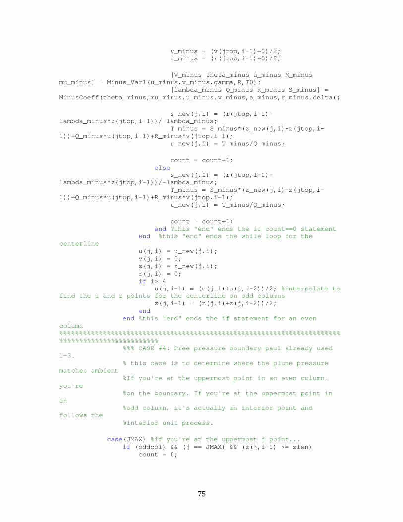
75

v_minus = (v(jtop,i-1)+0)/2; r_minus = (r(jtop,i-1)+0)/2; [V_minus theta_minus a_minus M_minus mu_minus] = Minus_Var1(u_minus,v_minus,gamma,R,T0); [lambda_minus Q_minus R_minus S_minus] = MinusCoeff(theta_minus,mu_minus,u_minus,v_minus,a_minus,r_minus,delta); z_new(j,i) = (r(jtop,i-1)-lambda_minus*z(jtop,i-1))/-lambda_minus; T_minus = S_minus*(z_new(j,i)-z(jtop,i-1))+Q_minus*u(jtop,i-1)+R_minus*v(jtop,i-1); u_new(j,i) = T_minus/Q_minus; count = count+1; else z_new(j,i) = (r(jtop,i-1)-lambda_minus*z(jtop,i-1))/-lambda_minus; T_minus = S_minus*(z_new(j,i)-z(jtop,i-1))+Q_minus*u(jtop,i-1)+R_minus*v(jtop,i-1); u_new(j,i) = T_minus/Q_minus; count = count+1; end %this "end" ends the if count==0 statement end %this "end" ends the while loop for the centerline u(j,i) = u_new(j,i); v(j,i) = 0; z(j,i) = z_new(j,i); r(j,i) = 0; if i>=4 u(j,i-1) = (u(j,i)+u(j,i-2))/2; %interpolate to find the u and z points for the centerline on odd columns z(j,i-1) = (z(j,i)+z(j,i-2))/2; end end %this "end" ends the if statement for an even column %%%%%%%%%%%%%%%%%%%%%%%%%%%%%%%%%%%%%%%%%%%%%%%%%%%%%%%%%%%%%%%%%%%%%%%%%%%%%%%%%%%%%%%%%%%%%%%% %%% CASE #4: Free pressure boundary paul already used 1-3. % this case is to determine where the plume pressure matches ambient %If you're at the uppermost point in an even column, you're %on the boundary. If you're at the uppermost point in an %odd column, it's actually an interior point and follows the %interior unit process. case(JMAX) %if you're at the uppermost j point... if (oddcol) && (j == JMAX) && (z(j,i-1) >= zlen) count = 0;

76

while abs(u(j,i)-u_new(j,i))>0.1 || abs(v(j,i)-v_new(j,i))>0.1 || abs(r(j,i)-r_new(j,i))>0.0001 || abs(z(j,i)-z_new(j,i))>0.0001; %tolerances suggested on p.603 of Z&H Vol I %Predict the point properties. if count==0; u_plus = u(jbot,i-1); v_plus = v(jbot,i-1); r_plus = r(jbot,i-1); u_minus = u(jtop,i-1); v_minus = v(jtop,i-1); r_minus = r(jtop,i-1); else u(j,i) = u_new(j,i); %Redefine the "corrected" values so that they're now the old values. v(j,i) = v_new(j,i); r(j,i) = r_new(j,i); z(j,i) = z_new(j,i); u_plus = (u(jbot,i-1)+u(j,i))/2; v_plus = (v(jbot,i-1)+v(j,i))/2; r_plus = (r(jbot,i-1)+r(j,i))/2; u_minus = (u(jtop,i-1)+u(j,i))/2; v_minus = (v(jtop,i-1)+v(j,i))/2; r_minus = (r(jtop,i-1)+r(j,i))/2; end [V_plus theta_plus a_plus M_plus mu_plus] = Plus_Var1(u_plus,v_plus,gamma,R,T0); [V_minus theta_minus a_minus M_minus mu_minus] = Minus_Var1(u_minus,v_minus,gamma,R,T0); [lambda_plus Q_plus R_plus S_plus] = PlusCoeff(theta_plus,mu_plus,u_plus,v_plus,a_plus,r_plus,delta); [lambda_minus Q_minus R_minus S_minus] = MinusCoeff(theta_minus,mu_minus,u_minus,v_minus,a_minus,r_minus,delta); if count==0; z(j,i) = (r(jtop,i-1)-lambda_minus*z(jtop,i-1)-r(jbot,i-1)+lambda_plus*z(jbot,i-1))/(lambda_plus-lambda_minus); r(j,i) = r(jbot,i-1)-lambda_plus*z(jbot,i-1)+lambda_plus*z(j,i); T_plus = S_plus*(z(j,i)-z(jbot,i-1))+Q_plus*u(jbot,i-1)+R_plus*v(jbot,i-1); T_minus = S_minus*(z(j,i)-z(jtop,i-1))+Q_minus*u(jtop,i-1)+R_minus*v(jtop,i-1); u(j,i) = (T_minus-(R_minus*T_plus/R_plus))/(Q_minus-(R_minus*Q_plus/R_plus)); v(j,i) = (T_plus-Q_plus*u(j,i))/R_plus; u_minus = (u(jtop,i-1)+u(j,i))/2;

77

v_minus = (v(jtop,i-1)+v(j,i))/2; r_minus = (r(jtop,i-1)+r(j,i))/2; u_plus = (u(jbot,i-1)+u(j,i))/2; v_plus = (v(jbot,i-1)+v(j,i))/2; r_plus = (r(jbot,i-1)+r(j,i))/2; [V_plus theta_plus a_plus M_plus mu_plus] = Plus_Var1(u_plus,v_plus,gamma,R,T0); [V_minus theta_minus a_minus M_minus mu_minus] = Minus_Var1(u_minus,v_minus,gamma,R,T0); [lambda_plus Q_plus R_plus S_plus] = PlusCoeff(theta_plus,mu_plus,u_plus,v_plus,a_plus,r_plus,delta); [lambda_minus Q_minus R_minus S_minus] = MinusCoeff(theta_minus,mu_minus,u_minus,v_minus,a_minus,r_minus,delta); z_new(j,i) = (r(jtop,i-1)-lambda_minus*z(jtop,i-1)-r(jbot,i-1)+lambda_plus*z(jbot,i-1))/(lambda_plus-lambda_minus); r_new(j,i) = r(jbot,i-1)-lambda_plus*z(jbot,i-1)+lambda_plus*z_new(j,i); T_plus = S_plus*(z_new(j,i)-z(jbot,i-1))+Q_plus*u(jbot,i-1)+R_plus*v(jbot,i-1); T_minus = S_minus*(z_new(j,i)-z(jtop,i-1))+Q_minus*u(jtop,i-1)+R_minus*v(jtop,i-1); u_new(j,i) = (T_minus-(R_minus*T_plus/R_plus))/(Q_minus-(R_minus*Q_plus/R_plus)); v_new(j,i) = (T_plus-Q_plus*u_new(j,i))/R_plus; count = count+1; else z_new(j,i) = (r(jtop,i-1)-lambda_minus*z(jtop,i-1)-r(jbot,i-1)+lambda_plus*z(jbot,i-1))/(lambda_plus-lambda_minus); r_new(j,i) = r(jbot,i-1)-lambda_plus*z(jbot,i-1)+lambda_plus*z_new(j,i); T_plus = S_plus*(z_new(j,i)-z(jbot,i-1))+Q_plus*u(jbot,i-1)+R_plus*v(jbot,i-1); T_minus = S_minus*(z_new(j,i)-z(jtop,i-1))+Q_minus*u(jtop,i-1)+R_minus*v(jtop,i-1); u_new(j,i) = (T_minus-(R_minus*T_plus/R_plus))/(Q_minus-(R_minus*Q_plus/R_plus)); v_new(j,i) = (T_plus-Q_plus*u_new(j,i))/R_plus; count = count+1; end end %This "end" ends the while loop. u(j,i) = u_new(j,i);

78

v(j,i) = v_new(j,i); r(j,i) = r_new(j,i); z(j,i) = z_new(j,i); end %This "end" ends the if statement for an odd column. %This is for a pressure boundary point if (evencol) && ((z(j,i-1) >= zlen) || Free == 1) count = 0; jbot=JMAX-1; Free = 1; %this is just to say we are now past the nozzle %plus values come from pt 2 relative to pt 4 on the %boundary. pt 4 is the pt being solved for u_plus = u(jbot,i-1);%(jbot,i-1); v_plus = v(jbot,i-1);%(jbot,i-1); r_plus = r(jbot,i-1);%(jbot,i-1); z_plus = z(jbot,i-1);%(jbot,i-1); %Minus values come from pt 3 relative to pt 4 on the %boundary. pt 4 is the pt being solved for %Minus values come from previous boundary calc. %either wall or boundary u_minus = u(j,i-2); v_minus = v(j,i-2); r_minus = r(j,i-2); z_minus = z(j,i-2); if z_plus > max(Zs) || z_plus < min (Zs) %must extrapolate is data point is out of range Pa = interp1(Zs,Ps,z_plus,'spline','extrap'); else Pa = interp1(Zs,Ps,z_plus,'spline','extrap'); end [V_plus theta_plus a_plus M_plus mu_plus] = Plus_Var1(u_plus,v_plus,gamma,R,T0);CP = gamma*R/(gamma-1); Q4 = (2.0*1*CP*T0*(1.0-(Pa/P0)^((gamma-1)/gamma)))^.5; Q = (u_plus^2+v_plus^2)^.5; A = atan(v_plus/u_plus); [M P rho T a] = THERMO(Q,GC,a_plus,gamma,R,P0,T0); lambda_plus = tan(A+asin(1.0/M)); % lambda0 = v_minus/u_minus; Q_plus = u_plus^2-a^2; R_plus = 2.0*u_plus*v_plus-Q_plus*lambda_plus; S_plus = delta*a^2*v_plus/r_plus; if imag(P)~=0 || isnan(P) > 0 || P == inf

79

display ('Pressure has gone to zero, infinity or imaginary') %pause end %These are here to start the while loop du = 10000; dv = 10000; z4 = (r_minus-r_plus-lambda0*z_minus+lambda_plus*z_plus)/(lambda_plus-lambda0); r4 = r_minus+lambda0*(z4-z_minus); T_plus = S_plus*(z4-z_plus)+Q_plus*u_plus+R_plus*v_plus; u4 = (Q_plus*T_plus-R_plus*(Q4^2*(Q_plus^2+R_plus^2)-T_plus^2)^.5)/(Q_plus^2+R_plus^2); v4 = (T_plus-Q_plus*u4)/R_plus; if imag (u4+v4) ~= 0 || u4 == 0 u4 = real(u4); v4 = real(v4); display('Caution! Imaginary elements in velocity guess detected.') end while abs(du)>0.1 || abs(dv)>0.1; count = count+1; zc = z4; rc = r4; uc = u4; vc = v4; if imag (u4+v4) ~= 0 || u4 == 0 error('Caution! code must be terminated due to reocurring imaginary values. Increase pressure ratio') end r(j,i) = 0.5*(r_plus+r4); u(j,i) = 0.5*(u_plus+u4); v(j,i) = 0.5*(v_plus+v4); Q = (u(j,i)^2+v(j,i)^2)^.5; A = atan(v(j,i)/u(j,i)); [M P rho T a] = THERMO(Q,GC,a_plus,gamma,R,P0,T0); if imag(P)~=0 || isnan(P) > 0 || P == inf error ('Caution! code must be terminated due to reocurring imaginary values. Increase pressure ratio') end lambda_plus = tan(A+asin(1/M)); Q_plus = u(j,i)^2-a^2; R_plus = 2.0*u(j,i)*v(j,i)-Q_plus*lambda_plus; S_plus = delta*a^2*v(j,i)/r(j,i); u(j,i) = 0.5*(u_minus+u4); v(j,i) = 0.5*(v_minus+v4); lambda0 = v(j,i)/u(j,i); z4 = (r_minus-r_plus-lambda0*z_minus+lambda_plus*z_plus)/(lambda_plus-lambda0); r4 = r_minus+lambda0*(z4-z_minus);

80

T_plus = S_plus*(z4-z_plus)+Q_plus*u_plus+R_plus*v_plus; u4 = (Q_plus*T_plus-R_plus*(Q4^2*(Q_plus^2+R_plus^2)-T_plus^2)^.5)/(Q_plus^2+R_plus^2); v4 = (T_plus-Q_plus*u4)/R_plus; du = u4-uc; dv = v4-vc; end %this ends the convergence while loop for this case %update values u(j,i) = u4; v(j,i) = v4; r(j,i) = r4; z(j,i) = z4; %%% %%% %%% Case for duct wall intersection point%%% %%% %%% if r4 >= rduct+tand(thetaduct)*(z4-zlen) %check if plume intersects duct wall count = 0; while count == 0 || abs(u(j,i)-u_new(j,i))>0.1 || abs(v(j,i)-v_new(j,i))>0.1 || abs(r(j,i)-r_new(j,i))>0.0001 || abs(z(j,i)-z_new(j,i))>0.0001; %tolerances suggested on p.603 of Z&H Vol I jbot=JMAX-1; %Predict the point properties. if count==0; u_plus = u(jbot,i-1); v_plus = v(jbot,i-1); r_plus = r(jbot,i-1); else u(j,i) = u_new(j,i); %Redefine the "corrected" values so that they're now the old values. v(j,i) = v_new(j,i); z(j,i) = z_new(j,i); r(j,i) = r_new(j,i); u_plus = (u(jbot,i-1)+u(j,i))/2; v_plus = (v(jbot,i-1)+v(j,i))/2; r_plus = (r(jbot,i-1)+r(j,i))/2; end [V_plus theta_plus a_plus M_plus mu_plus] = Plus_Var1(u_plus,v_plus,gamma,R,T0); [lambda_plus Q_plus R_plus S_plus] = PlusCoeff(theta_plus,mu_plus,u_plus,v_plus,a_plus,r_plus,delta); if count==0; if z(j,i)<zlen || imag(z(j,i))~=0 || z(j,i)<z(j,i-1)

81

possible_zees = roots([(0) (tand(thetaduct)-lambda_plus) (rduct-r(jbot,i-1)+lambda_plus*z(jbot,i-1))]); z(j,i) = max(possible_zees); %this line assumes one of the two roots will be positive and the other will be negative dr_dz = tand(thetaduct); r(j,i) = z(j,i-zlen)*dr_dz+rduct; else dr_dz = tand(thetaduct); r(j,i) = (z(j,i)-zlen)*dr_dz+rduct; end T_plus = S_plus*(z(j,i)-z(jbot,i-1))+Q_plus*u(jbot,i-1)+R_plus*v(jbot,i-1); u(j,i) = T_plus/(Q_plus+R_plus*dr_dz); v(j,i) = u(j,i)*dr_dz; u_plus = (u(jbot,i-1)+u(j,i))/2; v_plus = (v(jbot,i-1)+v(j,i))/2; r_plus = (r(jbot,i-1)+r(j,i))/2; [V_plus theta_plus a_plus M_plus mu_plus] = Plus_Var1(u_plus,v_plus,gamma,R,T0); [lambda_plus Q_plus R_plus S_plus] = PlusCoeff(theta_plus,mu_plus,u_plus,v_plus,a_plus,r_plus,delta); if z_new(j,i)<zlen || imag(z_new(j,i))~=0 || z_new(j,i)<z(j,i-1) || z_new(j,i)>2*zduct possible_zees = roots([(0) (tand(thetaduct)-lambda_plus) (rduct-r(jbot,i-1)+lambda_plus*z(jbot,i-1))]); z_new(j,i) = max(possible_zees); %this line assumes one of the two roots will be positive and the other will be negative dr_dz = tand(thetaduct); r_new(j,i) = (z_new(j,i)-zlen)*dr_dz+rduct; else dr_dz = tand(thetaduct); r_new(j,i) = (z_new(j,i)-zlen)*dr_dz+rduct; end T_plus = S_plus*(z_new(j,i)-z(jbot,i-1))+Q_plus*u(jbot,i-1)+R_plus*v(jbot,i-1); u_new(j,i) = T_plus/(Q_plus+R_plus*dr_dz); v_new(j,i) = u_new(j,i)*dr_dz; count = count+1; else

82

if z_new(j,i)<z_tr || imag(z_new(j,i))~=0 || z_new(j,i)<z(j,i-1) ||z_new(j,i) > zduct possible_zees = roots([(0) (tand(thetaduct)-lambda_plus) (rduct-r(jbot,i-1)+lambda_plus*z(jbot,i-1))]); z_new(j,i) = max(possible_zees); %this line assumes one of the two roots will be positive and the other will be negative dr_dz = tand(thetaduct); r_new(j,i) = (z_new(j,i)-zlen)*dr_dz+rduct; else dr_dz = tand(thetaduct); r_new(j,i) = (z_new(j,i)-zlen)*dr_dz+rduct; end T_plus = S_plus*(z_new(j,i)-z(jbot,i-1))+Q_plus*u(jbot,i-1)+R_plus*v(jbot,i-1); u_new(j,i) = T_plus/(Q_plus+R_plus*dr_dz); v_new(j,i) = u_new(j,i)*dr_dz; count = count+1; end end %This "end" ends the while loop u(j,i) = u_new(j,i); v(j,i) = v_new(j,i); r(j,i) = r_new(j,i); z(j,i) = z_new(j,i); r4 = r_new(j,i); z4 = z_new(j,i); end %This "end" ends the if statement for an duct intersection Rp(end+1) = r4; Zp(end+1) = z4; end %This "end" ends the if statement for an even column in fpb. %end %%% %%%%%%%%%%%%%%%%%%%%%%%%%%%%%%%%%%%%%%%%%%%%%%%%%%%%%%%%%%%%%%%%%%%%%%%%%%%%%%%%%%%%%%%%%%%%%%%%%%%%%%%%%%%%%%%%%%%%%%%%%%%%%%%%%%%%%%%%%%%%%%%% %CASE #2: WALL INTERSECTION %If you're at the uppermost point in an even column, you're %on the nozzle wall. If you're at the uppermost point in an

83

%odd column, it's actually an interior point and follows the %interior unit process. %case(JMAX) %if you're at the uppermost j point... if (oddcol) && (z(j,i-1) < zlen) count = 0; while abs(u(j,i)-u_new(j,i))>0.1 || abs(v(j,i)-v_new(j,i))>0.1 || abs(r(j,i)-r_new(j,i))>0.0001 || abs(z(j,i)-z_new(j,i))>0.0001; %tolerances suggested on p.603 of Z&H Vol I %Predict the point properties. if count==0; u_plus = u(jbot,i-1); v_plus = v(jbot,i-1); r_plus = r(jbot,i-1); u_minus = u(jtop,i-1); v_minus = v(jtop,i-1); r_minus = r(jtop,i-1); else u(j,i) = u_new(j,i); %Redefine the "corrected" values so that they're now the old values. v(j,i) = v_new(j,i); r(j,i) = r_new(j,i); z(j,i) = z_new(j,i); u_plus = (u(jbot,i-1)+u(j,i))/2; v_plus = (v(jbot,i-1)+v(j,i))/2; r_plus = (r(jbot,i-1)+r(j,i))/2; u_minus = (u(jtop,i-1)+u(j,i))/2; v_minus = (v(jtop,i-1)+v(j,i))/2; r_minus = (r(jtop,i-1)+r(j,i))/2; end [V_plus theta_plus a_plus M_plus mu_plus] = Plus_Var1(u_plus,v_plus,gamma,R,T0); [V_minus theta_minus a_minus M_minus mu_minus] = Minus_Var1(u_minus,v_minus,gamma,R,T0); [lambda_plus Q_plus R_plus S_plus] = PlusCoeff(theta_plus,mu_plus,u_plus,v_plus,a_plus,r_plus,delta); [lambda_minus Q_minus R_minus S_minus] = MinusCoeff(theta_minus,mu_minus,u_minus,v_minus,a_minus,r_minus,delta); if count==0; z(j,i) = (r(jtop,i-1)-lambda_minus*z(jtop,i-1)-r(jbot,i-1)+lambda_plus*z(jbot,i-1))/(lambda_plus-lambda_minus); r(j,i) = r(jbot,i-1)-lambda_plus*z(jbot,i-1)+lambda_plus*z(j,i); T_plus = S_plus*(z(j,i)-z(jbot,i-1))+Q_plus*u(jbot,i-1)+R_plus*v(jbot,i-1);

84

T_minus = S_minus*(z(j,i)-z(jtop,i-1))+Q_minus*u(jtop,i-1)+R_minus*v(jtop,i-1); u(j,i) = (T_minus-(R_minus*T_plus/R_plus))/(Q_minus-(R_minus*Q_plus/R_plus)); v(j,i) = (T_plus-Q_plus*u(j,i))/R_plus; u_minus = (u(jtop,i-1)+u(j,i))/2; v_minus = (v(jtop,i-1)+v(j,i))/2; r_minus = (r(jtop,i-1)+r(j,i))/2; u_plus = (u(jbot,i-1)+u(j,i))/2; v_plus = (v(jbot,i-1)+v(j,i))/2; r_plus = (r(jbot,i-1)+r(j,i))/2; [V_plus theta_plus a_plus M_plus mu_plus] = Plus_Var1(u_plus,v_plus,gamma,R,T0); [V_minus theta_minus a_minus M_minus mu_minus] = Minus_Var1(u_minus,v_minus,gamma,R,T0); [lambda_plus Q_plus R_plus S_plus] = PlusCoeff(theta_plus,mu_plus,u_plus,v_plus,a_plus,r_plus,delta); [lambda_minus Q_minus R_minus S_minus] = MinusCoeff(theta_minus,mu_minus,u_minus,v_minus,a_minus,r_minus,delta); z_new(j,i) = (r(jtop,i-1)-lambda_minus*z(jtop,i-1)-r(jbot,i-1)+lambda_plus*z(jbot,i-1))/(lambda_plus-lambda_minus); r_new(j,i) = r(jbot,i-1)-lambda_plus*z(jbot,i-1)+lambda_plus*z_new(j,i); T_plus = S_plus*(z_new(j,i)-z(jbot,i-1))+Q_plus*u(jbot,i-1)+R_plus*v(jbot,i-1); T_minus = S_minus*(z_new(j,i)-z(jtop,i-1))+Q_minus*u(jtop,i-1)+R_minus*v(jtop,i-1); u_new(j,i) = (T_minus-(R_minus*T_plus/R_plus))/(Q_minus-(R_minus*Q_plus/R_plus)); v_new(j,i) = (T_plus-Q_plus*u_new(j,i))/R_plus; count = count+1; else z_new(j,i) = (r(jtop,i-1)-lambda_minus*z(jtop,i-1)-r(jbot,i-1)+lambda_plus*z(jbot,i-1))/(lambda_plus-lambda_minus); r_new(j,i) = r(jbot,i-1)-lambda_plus*z(jbot,i-1)+lambda_plus*z_new(j,i); T_plus = S_plus*(z_new(j,i)-z(jbot,i-1))+Q_plus*u(jbot,i-1)+R_plus*v(jbot,i-1); T_minus = S_minus*(z_new(j,i)-z(jtop,i-1))+Q_minus*u(jtop,i-1)+R_minus*v(jtop,i-1);

85

u_new(j,i) = (T_minus-(R_minus*T_plus/R_plus))/(Q_minus-(R_minus*Q_plus/R_plus)); v_new(j,i) = (T_plus-Q_plus*u_new(j,i))/R_plus; count = count+1; end end %This "end" ends the while loop. u(j,i) = u_new(j,i); v(j,i) = v_new(j,i); r(j,i) = r_new(j,i); z(j,i) = z_new(j,i); end %This "end" ends the if statement for an odd column. if (evencol) && (((z(j,i-1) < zlen) && Free == 0)) %actual wall point count = 0; while abs(u(j,i)-u_new(j,i))>0.1 || abs(v(j,i)-v_new(j,i))>0.1 || abs(r(j,i)-r_new(j,i))>0.0001 || abs(z(j,i)-z_new(j,i))>0.0001; %tolerances suggested on p.603 of Z&H Vol I jbot=JMAX-1; %Predict the point properties. if count==0; u_plus = u(jbot,i-1); v_plus = v(jbot,i-1); r_plus = r(jbot,i-1); else u(j,i) = u_new(j,i); %Redefine the "corrected" values so that they're now the old values. v(j,i) = v_new(j,i); z(j,i) = z_new(j,i); r(j,i) = r_new(j,i); u_plus = (u(jbot,i-1)+u(j,i))/2; v_plus = (v(jbot,i-1)+v(j,i))/2; r_plus = (r(jbot,i-1)+r(j,i))/2; end [V_plus theta_plus a_plus M_plus mu_plus] = Plus_Var1(u_plus,v_plus,gamma,R,T0); [lambda_plus Q_plus R_plus S_plus] = PlusCoeff(theta_plus,mu_plus,u_plus,v_plus,a_plus,r_plus,delta); if count==0; %Assume to start out that the axial location is %still in the region of the throat arc. throat_arc = @(z_arc) (r(jbot,i-1)-lambda_plus*z(jbot,i-1)+sqrt(radius_of_curvature_downstream^2-z_arc^2)-r_th-radius_of_curvature_downstream+lambda_plus*z_arc); [z(j,i), low, high, iteration] = method_of_bisection(throat_arc,0,1e-10,z_tr,1e-12);

86

if z(j,i)>z_tr || z(j,i)==high || imag(z(j,i))~=0 || z(j,i)==low || z(j,i)<z(j,i-1) possible_zees = roots([(coeff_c) (coeff_b-lambda_plus) (coeff_a-r(jbot,i-1)+lambda_plus*z(jbot,i-1))]); z(j,i) = max(possible_zees); %this line assumes one of the two roots will be positive and the other will be negative [r(j,i) dr_dz] = AXI_Wall(z_tr,radius_of_curvature_downstream,r_th,coeff_a,coeff_b,coeff_c,z(j,i)); else [r(j,i) dr_dz] = AXI_Wall(z_tr,radius_of_curvature_downstream,r_th,coeff_a,coeff_b,coeff_c,z(j,i)); end T_plus = S_plus*(z(j,i)-z(jbot,i-1))+Q_plus*u(jbot,i-1)+R_plus*v(jbot,i-1); u(j,i) = T_plus/(Q_plus+R_plus*dr_dz); v(j,i) = u(j,i)*dr_dz; u_plus = (u(jbot,i-1)+u(j,i))/2; v_plus = (v(jbot,i-1)+v(j,i))/2; r_plus = (r(jbot,i-1)+r(j,i))/2; [V_plus theta_plus a_plus M_plus mu_plus] = Plus_Var1(u_plus,v_plus,gamma,R,T0); [lambda_plus Q_plus R_plus S_plus] = PlusCoeff(theta_plus,mu_plus,u_plus,v_plus,a_plus,r_plus,delta); throat_arc = @(z_arc) (r(jbot,i-1)-lambda_plus*z(jbot,i-1)+sqrt(radius_of_curvature_downstream^2-z_arc^2)-r_th-radius_of_curvature_downstream+lambda_plus*z_arc); [z_new(j,i), low, high, iteration] = method_of_bisection(throat_arc,0,1e-10,z_tr,1e-12); if z_new(j,i)>z_tr || z_new(j,i)==high || imag(z_new(j,i))~=0 || z(j,i)==low || z_new(j,i)<z(j,i-1) possible_zees = roots([(coeff_c) (coeff_b-lambda_plus) (coeff_a-r(jbot,i-1)+lambda_plus*z(jbot,i-1))]); z_new(j,i) = max(possible_zees); %this line assumes one of the two roots will be positive and the other will be negative [r_new(j,i) dr_dz] = AXI_Wall(z_tr,radius_of_curvature_downstream,r_th,coeff_a,coeff_b,coeff_c,z_new(j,i)); else [r_new(j,i) dr_dz] = AXI_Wall(z_tr,radius_of_curvature_downstream,r_th,coeff_a,coeff_b,coeff_c,z_new(j,i)); end T_plus = S_plus*(z_new(j,i)-z(jbot,i-1))+Q_plus*u(jbot,i-1)+R_plus*v(jbot,i-1);

87

u_new(j,i) = T_plus/(Q_plus+R_plus*dr_dz); v_new(j,i) = u_new(j,i)*dr_dz; count = count+1; else throat_arc = @(z_arc) (r(jbot,i-1)-lambda_plus*z(jbot,i-1)+sqrt(radius_of_curvature_downstream^2-z_arc^2)-r_th-radius_of_curvature_downstream+lambda_plus*z_arc); [z_new(j,i), low, high, iteration] = method_of_bisection(throat_arc,0,1e-10,z_tr,1e-12); if z_new(j,i)>z_tr || z_new(j,i)==high || imag(z_new(j,i))~=0 || z_new(j,i)==low || z_new(j,i)<z(j,i-1) possible_zees = roots([(coeff_c) (coeff_b-lambda_plus) (coeff_a-r(jbot,i-1)+lambda_plus*z(jbot,i-1))]); z_new(j,i) = max(possible_zees); %this line assumes one of the two roots will be positive and the other will be negative [r_new(j,i) dr_dz] = AXI_Wall(z_tr,radius_of_curvature_downstream,r_th,coeff_a,coeff_b,coeff_c,z_new(j,i)); else [r_new(j,i) dr_dz] = AXI_Wall(z_tr,radius_of_curvature_downstream,r_th,coeff_a,coeff_b,coeff_c,z_new(j,i)); end T_plus = S_plus*(z_new(j,i)-z(jbot,i-1))+Q_plus*u(jbot,i-1)+R_plus*v(jbot,i-1); u_new(j,i) = T_plus/(Q_plus+R_plus*dr_dz); v_new(j,i) = u_new(j,i)*dr_dz; count = count+1; end end %This "end" ends the while loop u(j,i) = u_new(j,i); v(j,i) = v_new(j,i); r(j,i) = r_new(j,i); z(j,i) = z_new(j,i); end %This "end" ends the if statement for an even column. %%%%%%%%%%%%%%%%%%%%%%%%%%%%%%%%%%%%%%%%%%%%%%%%%%%%%%%%%%%%%%%%%%%%%%%%%%%%%%%%%%%%%%%%%%%%%%%%%%%%%%%%%%%%%%%%%%%%%%%%%%%%%%%%%%%%%%%%%%%% %%%%%%%%%%%%%%%%%%%%%%%%%%%%%%%%%%%%%%%%%%%%%%%%%%%%%%%%%%%%%%%%%%%%%%%%%%%%%%%%%%%%%%%%%%%%%%%%%%%%%%%%%%%%%%%%%%%%%%%%%%%%%%%%%% %CASE #3: INTERIOR POINTS (fall neither on the centerline or the nozzle %wall) otherwise count=0;

88

while abs(u(j,i)-u_new(j,i))>0.1 || abs(v(j,i)-v_new(j,i))>0.1 || abs(r(j,i)-r_new(j,i))>0.0001 || abs(z(j,i)-z_new(j,i))>0.0001; %tolerances suggested on p.603 of Z&H Vol I %Predict the point properties. if count==0; u_plus = u(jbot,i-1); v_plus = v(jbot,i-1); if j==2; if oddcol r_plus = r(jtop,i-1)/100; %can't use r_plus(j,i)=r(jbot,i-1) because it would result in a divide by zero else r_plus = r(jbot,i-1); end else r_plus = r(jbot,i-1); end u_minus = u(jtop,i-1); v_minus = v(jtop,i-1); r_minus = r(jtop,i-1); else u(j,i) = u_new(j,i); %Redefine the "corrected" values so that they're now the old values. v(j,i) = v_new(j,i); z(j,i) = z_new(j,i); r(j,i) = r_new(j,i); u_plus = (u(jbot,i-1)+u(j,i))/2; v_plus = (v(jbot,i-1)+v(j,i))/2; r_plus = (r(jbot,i-1)+r(j,i))/2; u_minus = (u(jtop,i-1)+u(j,i))/2; v_minus = (v(jtop,i-1)+v(j,i))/2; r_minus = (r(jtop,i-1)+r(j,i))/2; end [V_plus theta_plus a_plus M_plus mu_plus] = Plus_Var1(u_plus,v_plus,gamma,R,T0); [V_minus theta_minus a_minus M_minus mu_minus] = Minus_Var1(u_minus,v_minus,gamma,R,T0); [lambda_plus Q_plus R_plus S_plus] = PlusCoeff(theta_plus,mu_plus,u_plus,v_plus,a_plus,r_plus,delta); [lambda_minus Q_minus R_minus S_minus] = MinusCoeff(theta_minus,mu_minus,u_minus,v_minus,a_minus,r_minus,delta); if count==0; z(j,i) = (r(jtop,i-1)-lambda_minus*z(jtop,i-1)-r(jbot,i-1)+lambda_plus*z(jbot,i-1))/(lambda_plus-lambda_minus); r(j,i) = r(jbot,i-1)-lambda_plus*z(jbot,i-1)+lambda_plus*z(j,i);

89

T_plus = S_plus*(z(j,i)-z(jbot,i-1))+Q_plus*u(jbot,i-1)+R_plus*v(jbot,i-1); T_minus = S_minus*(z(j,i)-z(jtop,i-1))+Q_minus*u(jtop,i-1)+R_minus*v(jtop,i-1); u(j,i) = (T_minus-(R_minus*T_plus/R_plus))/(Q_minus-(R_minus*Q_plus/R_plus)); v(j,i) = (T_plus-Q_plus*u(j,i))/R_plus; u_minus = (u(jtop,i-1)+u(j,i))/2; v_minus = (v(jtop,i-1)+v(j,i))/2; r_minus = (r(jtop,i-1)+r(j,i))/2; u_plus = (u(jbot,i-1)+u(j,i))/2; v_plus = (v(jbot,i-1)+v(j,i))/2; r_plus = (r(jbot,i-1)+r(j,i))/2; [V_plus theta_plus a_plus M_plus mu_plus] = Plus_Var1(u_plus,v_plus,gamma,R,T0); [V_minus theta_minus a_minus M_minus mu_minus] = Minus_Var1(u_minus,v_minus,gamma,R,T0); [lambda_plus Q_plus R_plus S_plus] = PlusCoeff(theta_plus,mu_plus,u_plus,v_plus,a_plus,r_plus,delta); [lambda_minus Q_minus R_minus S_minus] = MinusCoeff(theta_minus,mu_minus,u_minus,v_minus,a_minus,r_minus,delta); z_new(j,i) = (r(jtop,i-1)-lambda_minus*z(jtop,i-1)-r(jbot,i-1)+lambda_plus*z(jbot,i-1))/(lambda_plus-lambda_minus); r_new(j,i) = r(jbot,i-1)-lambda_plus*z(jbot,i-1)+lambda_plus*z_new(j,i); T_plus = S_plus*(z_new(j,i)-z(jbot,i-1))+Q_plus*u(jbot,i-1)+R_plus*v(jbot,i-1); T_minus = S_minus*(z_new(j,i)-z(jtop,i-1))+Q_minus*u(jtop,i-1)+R_minus*v(jtop,i-1); u_new(j,i) = (T_minus-(R_minus*T_plus/R_plus))/(Q_minus-(R_minus*Q_plus/R_plus)); v_new(j,i) = (T_plus-Q_plus*u_new(j,i))/R_plus; count = count+1; else z_new(j,i) = (r(jtop,i-1)-lambda_minus*z(jtop,i-1)-r(jbot,i-1)+lambda_plus*z(jbot,i-1))/(lambda_plus-lambda_minus); r_new(j,i) = r(jbot,i-1)-lambda_plus*z(jbot,i-1)+lambda_plus*z_new(j,i); T_plus = S_plus*(z_new(j,i)-z(jbot,i-1))+Q_plus*u(jbot,i-1)+R_plus*v(jbot,i-1); T_minus = S_minus*(z_new(j,i)-z(jtop,i-1))+Q_minus*u(jtop,i-1)+R_minus*v(jtop,i-1);

90

u_new(j,i) = (T_minus-(R_minus*T_plus/R_plus))/(Q_minus-(R_minus*Q_plus/R_plus)); v_new(j,i) = (T_plus-Q_plus*u_new(j,i))/R_plus; count = count+1; end %This "end" ends the if statement. end %This "end" ends the while loop. u(j,i) = u_new(j,i); v(j,i) = v_new(j,i); r(j,i) = r_new(j,i); z(j,i) = z_new(j,i); end %This "end" ends the switch statement. %%%%%%%%%%%%%%%%%%%%%%%%%%%%%%%%%%%%%%%%%%%%%%%%%%%%%%%%%%%%%%%%%%%%%%%%%%%%%%%%%%%%%%%%%%%%%%%%%%%%%%%%%%%%%%%%%%%%%%%%%%%%%%%%%%%%%%% % Check to see if you're done. if (z(JMAX,i)>=zduct) || (i >= IMAX) || (Free == 1 && ((Rp(end) < max(Rp)-max(Rp)/75) || max(Rp) >= rduct+tand(thetaduct)*(max(Zp)-zlen))); %this will make sure you're at the end of the nozzle. may still be in the duct if (mod(i,2)==0); done = true; end end end %This "end" ends the for loop for j end %This "end" ends the while loop for i i_end = i-1; %Calculate the state properties. Zp = Zp(1:length(Zp-1)); Rp = Rp(1:length(Rp-1)); V = zeros(JMAX,i_end); a = zeros(JMAX,i_end); M = zeros(JMAX,i_end); P = zeros(JMAX,i_end); T = zeros(JMAX,i_end); for j=1:JMAX for i=1:i_end V(j,i)=sqrt(u(j,i)^2+v(j,i)^2); a(j,i)=speed_of_sound(gamma,R,T0,V(j,i)); M(j,i)=V(j,i)/a(j,i); P(j,i)= P0/(1+((gamma-1)/2)*M(j,i)^2)^(gamma/(gamma-1)); T(j,i)=T0/(1+((gamma-1)/2)*M(j,i)^2); end end mdot = 32.2*(2*r_th*P0/((gamma*R*T0)^.5))*gamma*(2/(gamma+1))^((gamma+1)/(2*(gamma-1))); %[lbm/ft-s] coeffs = [coeff_a; coeff_b; coeff_c];

91

function [Ms Ps Zs mdotstar Zd Rd Pd Md At] = SSFLOW2(Zp,Rp,Zl,Rl,rduct,thetaduct,gamma,pa,Ta,R,rhoa,intfigs,tb) %%%%Inputs %Zp plume boundary location in axial direction [ft] %Rp plume boundary location in transverse direction from centerline [ft] %Zl nozzle lip location in axial direction [ft] %Rl nozzle lip location in transverse direction [ft] %rduct duct half width from centerline [ft] %thetaduct Diverging angle of duct %gamma Ratio of specific heats %pa Ambient inlet pressure [lbf/ft^2] %Ta Ambient inlet Temperature [R] %R Gas constant %rhoa Ambient inlet density [slug/ft3] %intfigs chroniker for intermediate figures %tb Thickness of nozzle lip %%%%Outputs %Ms Secondary Mach Number Distribution %Ps Secondary Pressure Distribution [lbf/ft2] %Zs Streamwise location corresponding to pressure and Mach numbers [ft] %mdotstar Mass flowrate of secondary stream [lbm/s-ft] % %%%% Plotting outputs %Zd %Rd Coordinates of duct walls %Pd Vector of pressures of secondary flow %Md Vector of Mach numbers of secondary flow %At Secondary Aerodynamic throat width Rl = Rl+tb; %correct for nozzle base thickness M = zeros(length(Zp)+2,1); P = zeros(size(M)); RD(1:2) = rduct; RD(3:length(M)) = rduct+(Zp-Zl)*tand(thetaduct); A = zeros(size(M)); A(1:2) = RD(1:2)-Rl; A(3:length(Rp)+2) = RD(3:length(Rp)+2)-Rp(1:length(Rp)); for i=1:length (A) if A(i) > A(1) A(i) = A(1); end if A(i) <= 0 A(i) = eps; display('primary plume intersects duct wall') end end

92

At = min(A); %determine the throat dimensions for i = 1:length(A) if A(i) == min (A) t = i; end end M(t) = 1.0; P(t) = pa*(2/(gamma+1))^(gamma/(gamma-1)); rhostar = rhoa*32.2/(1+(gamma-1)/2)^(1/(gamma-1)); %[lbm/s/ft] Tstar = Ta/(1+(gamma-1)/2); Vstar = (gamma*R*Tstar)^0.5; mdotstar = rhostar*At*Vstar; %[lbm/ft-s] if min(A) <= eps M(t) = 0; else for i = 1:t-1 M(i) = fminbnd(@(Mi) abs(1/Mi*((2/(gamma+1))*(1+(gamma-1)*Mi^2/2))^((gamma+1)/(2*(gamma-1)))-A(i)/At), .01, .99 ); end for i = t+1:length(A) M(i) = fzero(@(Mi) 1/Mi*((2/(gamma+1))*(1+(gamma-1)*Mi^2/2))^((gamma+1)/(2*(gamma-1)))-A(i)/At, .9 ); end end %Next relate pressure to Mach using isentropic relations %THe final step is to plot the outputs. %in order to do this, we need a mesh of points, %to do this we augement the Rp,Zp,P and M vectors to make them matricies %simply add the points along the ejector shroud in the same z location %in short, duplicate Zp,P and M column in the next row %New Rp column is half width of duct. Zd = zeros(length(Zp)+2,2); Rd = zeros(size(Zd)); Md = zeros(size(Zd)); Zd(1,:) = 0; Zd(2,:) = Zl; Zd(3:end,1) = Zp(1:end); Zd(3:end,2) = Zp(1:end); Rd(1:2,1) = Rl; Rd(3:end,1) = Rp(1:end); for i=1:length(Rd) if Rd(i,1) < Rl Rd(i,1) = Rl; end end Rd(:,2) = RD; Md(:,1) = M(1:end); Md(:,2) = M(1:end); %Find pressures using isentropic relations

93

Pd = pa./(1+((gamma-1)/2).*Md.^2).^(gamma/(gamma-1)); Ps = []; Ms = []; Zs = []; Ms = Md(:,1); Ps = Pd(:,1); Zs = Zd(:,1); if intfigs ==1 % %Generate plots % hold on % %figure % surf(Zd,Rd,Pd)%,z,r,Pp) % title('Pressure Distribution of Secondary Flow [lbf/ft2]') % %axis([0,.70,.0,.25,350,600]) % colorbar % hold off hold on %figure surf(12*Zd,12*Rd,Md) title('Mach number of secondary flow') %axis([0,.70,.0,.25,0,1]) %colorbar view(2) %hold off %hold on % surf(12*Zd,12*Rd,Pd) %view(2) else end %Initial Data Line %This function generates an initial data line using Kliegel's method. The method of %characteristics can begin once an initial data line is determined. Kliegel's method is a modified %version of Hall's method that is capable of handling throats with a ratio of upstream throat radius %of curvature to throat radius that is less than 1. function [x y u_tilda v_tilda] = KliegelDataLine(gamma,gas_constant,curvature_upstream,r_star,T0,JMAX) % gamma = ratio of specific heats for the working fluid (combustion products of LOX and LH2 in the case of SSME) % gas_constant = gas constant for the working fluid (ft-lbf/slug R) % curvature_upstream = radius of curvature immediately upstream from the throat (ft)

94

% r_star = throat radius (ft) % T0 = chamber stagnation temperature (deg R) % JMAX = number of points in the initial column T_star = (2/(1+gamma))*T0; %throat temperature (deg R) a_star = sqrt(gamma*gas_constant*T_star); %throat speed of sound (ft/s) R = curvature_upstream/r_star; %EXPANSION PARAMETER y = linspace(0,r_star,JMAX)'; %this is the span of transverse points from the axis to the throat wall r = y./r_star; %this is y non-dimensionalized by the value of the throat radius z = 0.25 - 0.25.*r.^2; %this is the axial non-dimensional value that corresponds to r x = (r_star.*z)/sqrt((2*R)/(gamma+1)); %this is the span of axial points corresponding to y u1 = 0.5.*(r.^2)-0.25+z; %v1 = 0.25.*(r.^3)-(0.25.*r)+(r.*z); v1 = 0; %Assume v1 contributes negligibly u2 = (((2*gamma+9)/24).*r.^4)-(((4*gamma+15)/24).*r.^2)+((10*gamma+57)/288)+z.*(r.^2-(5/8))-(((2*gamma-3)/6).*z.^2); %Z&H Vol II Eq. 15.102 v2 = (((gamma+3)/9).*r.^5)-(((20*gamma+63)/96).*r.^3)+(((28*gamma+93)/288).*r)+z.*((((2*gamma+9)/6).*r.^3)-(((4*gamma+15)/12).*r))+(r.*z.^2); %Z&H Vol II Eq. 15.103 %u3 = (((556*gamma^2+1737*gamma+3069)/10368).*r.^6)-(((388*gamma^2+1161*gamma+1881)/2304).*r.^4)+(((304*gamma^2+831*gamma+1242)/1728).*r.^2)-((2708*gamma^2+7839*gamma+14211)/82944)+z.*((((52*gamma^2+51*gamma+327)/384).*r.^4)-(((52*gamma^2+75*gamma+279)/192).*r.^2)+(((92*gamma^2+180*gamma+639)/1152)))+z.^2.*((((-7*gamma-3)/8).*r.^2)+((13*gamma-27)/48))+(((4*gamma^2-57*gamma+27)/144).*z.^3); %Z&H Vol II Eq. 15.104 u3 = (((556*gamma^2+1737*gamma+3069)/10368).*r.^6)-(((388*gamma^2+1161*gamma+1881)/2304).*r.^4)+(((304*gamma^2+831*gamma+1242)/1728).*r.^2)... -((2708*gamma^2+7839*gamma+14211)/82944)+z.*((((52*gamma^2+51*gamma+327)/384).*r.^4)-(((52*gamma^2+75*gamma+279)/192).*r.^2)... +(((200*gamma^2+72*gamma+639)/1152)))+z.^2.*((((-7*gamma-3)/8).*r.^2)+((13*gamma-27)/48))+(((4*gamma^2-57*gamma+27)/144).*z.^3); %Hall Eq. 81 %v3 = (((6836*gamma^2+23031*gamma+30627)/82944).*r.^7)-(((3380*gamma^2+11391*gamma+15291)/13824).*r.^5)+(((3424*gamma^2+11271*gamma+15228)/13824).*r.^3)-(((7100*gamma^2+22311*gamma+30249)/82944).*r)+z.*((((556*gamma^2+1737*gamma+3069)/1728).*r.^5)-(((388*gamma^2+1161*gamma+1881)/576).*r.^3)+(((304*gamma^2+831*gamma+1242)/864).*r))+z.^2.*((((52*gamma^2+51*gamma+327)/192).*r.^3)-(((52*gamma^2+75*gamma+279)/192).*r))-z.^3.*(((7*gamma-3)/12).*r); %Z&H Vol II Eq. 15.105

95

v3 = (((6836*gamma^2+23031*gamma+30627)/82944).*r.^7)-(((3380*gamma^2+11391*gamma+15291)/13824).*r.^5)... +(((3748*gamma^2+10947*gamma+15228)/13824).*r.^3)-(((9044*gamma^2+20367*gamma+30249)/82944).*r)... +z.*((((556*gamma^2+1737*gamma+3069)/1728).*r.^5)-(((388*gamma^2+1161*gamma+1881)/576).*r.^3)... +(((304*gamma^2+831*gamma+1242)/864).*r))+z.^2.*((((52*gamma^2+51*gamma+327)/192).*r.^3)... -(((52*gamma^2+75*gamma+279)/192).*r))-z.^3.*(((7*gamma-3)/12).*r); %Hall Eq. 82 u_tilda = a_star*(1+((R+1)^-1).*u1+((R+1)^-2).*(u1+u2)+((R+1)^-3).*(u1+2.*u2+u3)); %Z&H Vol II Eq. 15.106 v_tilda = a_star*sqrt((gamma+1)/(2*(R+1)))*(((R+1)^-1).*v1+((R+1)^-2).*(1.5.*v1+v2)+((R+1)^-3).*((15/8).*v1+(5/2).*v2+v3)); %Z&H Vol II Eq. 15.107 function [V_minus theta_minus a_minus M_minus mu_minus] = Minus_Var1(u_minus,v_minus,gamma,R,T0) V_minus = sqrt(u_minus^2 + v_minus^2); theta_minus = atan(v_minus/u_minus); a_minus = speed_of_sound(gamma,R,T0,V_minus); M_minus = V_minus/a_minus; mu_minus = mach_angle(M_minus); end function [lambda_minus Q_minus R_minus S_minus] = MinusCoeff(theta_minus,mu_minus,u_minus,v_minus,a_minus,r_minus,delta) lambda_minus = tan(theta_minus-mu_minus); Q_minus = u_minus^2-a_minus^2; R_minus = 2*u_minus*v_minus-Q_minus*lambda_minus; S_minus = delta*a_minus^2*v_minus/r_minus; end function [lambda_plus Q_plus R_plus S_plus] = PlusCoeff(theta_plus,mu_plus,u_plus,v_plus,a_plus,r_plus,delta) lambda_plus = tan(theta_plus+mu_plus); Q_plus = u_plus^2-a_plus^2; R_plus = 2*u_plus*v_plus-Q_plus*lambda_plus; S_plus = delta*a_plus^2*v_plus/r_plus; end function [V_plus theta_plus a_plus M_plus mu_plus] = Plus_Var1(u_plus,v_plus,gamma,R,T0) V_plus = sqrt(u_plus^2 + v_plus^2);

96

theta_plus = atan(v_plus/u_plus); a_plus = speed_of_sound(gamma,R,T0,V_plus); M_plus = V_plus/a_plus; mu_plus = mach_angle(M_plus); end %This portion correlates to the Z&H example. R may be different units. %mu_plus is also named alpha_plus function [M P R T C] = THERMO(Q,GC,CP,gamma,RG,P0,T0) %This sub code has unit issues CP = gamma*RG/(gamma-1); %CP is Cp not speed-of-sound_pluss GC = 1; %this solves a unit issue (thermo requires RG in ftlbf/lbmR. input as ftlbf/slugR=ft^2/Rs^2) T = T0-Q^2/(2*GC*CP); C = (gamma*GC*RG*T)^.5; %speed of sound %this value is too large by a magnitude M = Q/C; P = P0*(T/T0)^(gamma/(gamma-1));%was 144 cf, R = P/(RG*T)*32.2; %density. 32.2 added to change slugs to lbm function acoustic_speed = speed_of_sound(gamma,R,T0,V) %This function calculates the local speed of sound. %gamma is the ratio of specific heats. %R is the gas constant. %T0 is the stagnation temperature. %V is the local velocity. acoustic_speed = sqrt(gamma*R*T0-((gamma-1)/2)*V^2); end

numerical examination of flow field characteristics and

Documents