numerical blow-up for the porous medium equation with a sourcemate.dm.uba.ar/~pgroisma/poros.pdf ·...
TRANSCRIPT

Numerical blow-up for the porous mediumequation with a source
Raul Ferreira ∗
Departamento de Matematicas, U. Autonoma de Madrid28049 Madrid, Spain.
e-mail: [email protected]
Pablo Groisman †
Departamento de Matematica, F.C.E y N., UBA(1428) Buenos Aires, Argentina.
e-mail: [email protected]
Julio D. Rossi †
Departamento de Matematica, F.C.E y N., UBA(1428) Buenos Aires, Argentina.e-mail: [email protected]
Abstract
We study numerical approximations of positive solutions of the porous mediumequation with a nonlinear source,
ut = (um)xx + up, (x, t) ∈ (−L, L)× (0, T ),u(−L, t) = u(L, t) = 1, t ∈ [0, T ),u(x, 0) = ϕ(x),≥ 1 x ∈ (−L, L),
where m > 1, p > 0 and L > 0 are parameters. We describe in terms of p, m, andL when solutions of a semidiscretization in space exist globally in time and whenthey blow up in a finite time. We also find the blow-up rates and the blow-up sets,proving that there is no regional blow-up for the numerical scheme.
∗Partially supported by DGES Project PB94-0153 and EU Programme TMR FMRX-CT98-0201.†Supported by Universidad de Buenos Aires under grant EX046, CONICET (Argentina) and Fun-
dacion Antorchas.AMS Subject Classification: 35B40, 65M12, 65M06.Keywords and phrases: numerical blow-up, porous medium equation.
1
1 Introduction.
In this paper we deal with numerical approximations of the following problem
ut = (um)xx + up, (x, t) ∈ (−L,L)× [0, T ),u(−L, t) = u(L, t) = 1, t ∈ [0, T ),u(x, 0) = ϕ(x) ≥ 1, x ∈ (−L,L),
(1.1)
where m > 1 and p > 0 are parameters. Problem (1.1) can be thought as a model fornonlinear heat propagation. In this case u stands for the temperature and we are inpresence of reaction (giving by the power up).
We assume that ϕ is smooth and compatible with the boundary conditions in order toobtain a regular solution. Also, for simplicity, we assume that ϕ is a bell shaped function,that is, ϕ is symmetric, ϕ(x) = ϕ(−x) for x > 0, and decreasing in [0, L]. These symmetryproperties will be preserved by our numerical scheme and make computations easier.
For many differential equations or systems the solutions can become unbounded infinite time, a phenomenon that is known as blow-up. Typical examples where this happensare parabolic problems involving nonlinear reaction terms, like (1.1). The solution of (1.1)only exists for a finite period of time (T <∞, in this case u becomes unbounded in finitetime and we say that it has blow-up) or it is defined for all positive t (T = ∞, in thiscase we call it a global solution). These problems have been widely analyzed from amathematical point of view (see for example [SGKM], [P], [L] and the references therein)but, only few results concerning the numerical approximation of them can be found in theliterature (we refer for example to [ALM1], [ALM2], [BB], [BK], [BHR], [DER], [FBR]).Indeed, even for an elementary ordinary differential equation y ′ = f(y) having blow-up,the usual analysis to obtain error estimates and adaptive step procedures do not applybecause they are based on regularity assumptions which are not satisfied in this case.
Here we analyze numerical approximations of blowing up solutions. By a semidis-cretization in space we obtain a system of ordinary differential equations which is expectedto be an approximation of the original problem. Our objective is to analyze whether thissystem has a similar behaviour than the original problem.
The nonlinear diffusion that we are considering here, (um−1ux)x, degenerates at levelu = 0, giving only weak solutions if we allow the initial data (or the boundary conditions)to vanish. Since we are interested in blowing up solutions, we avoid this lack of regularityimposing ϕ ≥ 1 and u(−L, t) = u(L, t) = 1. This gives us regular solutions (see [LSU]).
We want to remark that all our results are valid for regular solutions of problems ofthe form ut = (φ(u))xx+f(u) if we impose that φ(u) ∼ um and f(u) ∼ up when u becomeslarge. To simplify the exposition we state and prove our results for (1.1).
Let us resume what is known for continuos problem (1.1) (see [SGKM] and referencestherein),
2

(i) If p > m there exists blowing up solutions for initial data u0 large enough. The
blow-up rate is given by ‖u(·, t)‖∞ ∼ (T − t)−1
p−1 and the blow-up set is a single pointx = 0 (this means that u remains bounded away from the origin).
(ii) If p = m the existence of blowing up solutions depends on the length of theinterval. Let λ1(L) = π/2L be the first eigenvalue of the Laplacian in [−L,L]. Then,every solution blows up if and only if λ1(L) < 1. That is, if L > π/2 every positive
solution blows up and the blow-up rate is given by ‖u(·, t)‖∞ ∼ (T − t)−1
m−1 . In this caseit is known that the blow-up set is given by
B(u) =
{
[−L,L] if π/2 < L ≤ mπ/(m− 1),(−mπ/(m− 1),mπ/(m− 1)) if L > mπ/(m− 1).
Moreover, there exists a self-similar profile, z(x), that gives the asymptotic behaviour foru near T in the form,
limt↗T
(T − t)1
m−1u(x, t) = z(x).
Let us remark that if L > mπ/(m− 1) the support of z is the interval
(
−mπ
(m− 1),
mπ
(m− 1)
)
.
Therefore we have regional blow-up for large values of L. On the other hand, if L ≤ π/2every solution is global.
(iii) If p < m every solution is global.
Now we introduce the numerical scheme. We discretize using piecewise linear finiteelements with mass lumping in a uniform mesh for the space variable (it is well knownthat this discretization in space coincides with the classic central finite difference secondorder scheme), see [Ci]. Mass lumping is widely used in parabolic problems with blow-up,see for example [ALM1], [ALM2], [Ch], [DER], [N], [NU].
We denote with U(t) = (u−N(t), ...., uN (t)) the values of the numerical approximationat the nodes xi = ih (h = L/N) at time t. Then U(t) verifies the following equation:
MU ′(t) = −AUm(t) +MU p(t),u−N(t) = uN(t) = 1,U(0) = ϕI ,
(1.2)
where M is the mass matrix obtained with lumping, A is the stiffness matrix and ϕI isthe Lagrange interpolation of the initial datum, ϕ. Writing this equation explicitly we
3
obtain the following ODE system,
u−N(t) = 1,
u′k(t) =1
h2(um
k+1(t)− 2umk (t) + um
k−1(t)) + upk(t),
uN(t) = 1,
uk(0) = ϕ(xk), −N + 1 ≤ k ≤ N − 1.
(1.3)
First we state a convergence result that says that for any positive τ , the methodconverges uniformly in sets of the form [−L,L] × [0, T − τ ]. Let us observe that, sincesolutions are blowing up in L∞ norm, it is natural to consider uniform convergence. Sincethe solution develops a singularity at time t = T we cannot expect that the convergenceresult extends up to T .
Theorem 1.1 Let u(x, t) ∈ C4,1([−L,L] × [0, T − τ ]) be a positive solution of (1.1) andU(t) the numerical approximation given by (1.3). Then, there exists a constant C, thatdepends on the C4,1([−L,L] × [0, T − τ ]) norm of u, such that for every h small enoughit holds
maxt∈[0,T−τ ]
maxk|u(xk, t)− uk(t)| ≤ Ch2.
Next we begin with the analysis of the asymptotic behaviour of solutions of (1.3).Next theorem describes when (1.3) has solutions with blow-up. To do this, we introduceλ1(L, h) that stands for the first discrete eigenvalue for the Laplacian, that is the firsteigenvalue of the problem
{
AΨ = λMΨ,Ψ−N = ΨN = 0.
(1.4)
Let us recall that
λ1(L, h) =( π
2L
)2
+O(h2),
see [FG].
Theorem 1.2 There exists blowing up solutions for (1.3) if and only if p > m or p = mwith λ1(L, h) < 1. Moreover, in case p = m with λ1(L, h) < 1 every nontrivial solutionblows up. In case p > m and ϕ an initial data such that the solution u of problem (1.1)blows up then U also blows up for every h small enough.
This theorem shows that the numerical scheme reproduces the blow-up cases in a veryaccurate way. Let us remark that λ1(L, h) → λ1(L) as h→ 0.
Numerical blow-up has been studied before. In [ALM1], [ALM2], [BK], [BHR], [Ch],[N], [GR] the semilinear heat equation is considered. See also [LR] for a time discretizationof (1.1).
4

As a consequence of our blow-up results we can get bounds on the time remaining toachieve the numerical blow-up time in terms of U(t). This allows us to prove that thenumerical blow-up time Th converges to T when h goes to zero.
Corollary 1.1 Let ϕ be an initial datum for (1.1) such that u blows up, if we call T andTh the blow-up times for u and uh respectively, we have
limh→0
Th = T.
Now we describe the blow-up rate for the numerical scheme.
Theorem 1.3 Let U(t) be a blowing up solution of (1.3) and Th its blow-up time, thenthere exists two positive constants Ci = Ci(h) such that
C1(Th − t)−1/(p−1) ≤ ‖U‖∞(t) ≤ C2(Th − t)−1/(p−1).
Moreover, if p > m there holds,
limt↗Th
(Th − t)1/(p−1)‖U‖∞(t) = Cp =
(
1
p− 1
)1/(p−1)
.
We remark that this rate coincides with the blow-up rate of the continuous problem(1.1).
With the blow-up rate we can characterize the numerical blow-up set, that is the setof nodes xk such that uk(t) → +∞ when t↗ Th.
Theorem 1.4 Let U(t) be a blowing up solution of (1.3) which blows up at time Th, then
1. For p > m the blow-up set is given by a finite number of nodes, i.e.,
B(U) = [−Kh, Kh],
where K ≡ K(p,m) is the only integer that verifies the following expression,
∑K+1i=0 mi
∑Ki=0m
i< p ≤
∑Ki=0m
i
∑K−1i=0 mi
, that is, K =
[
ln((p− 1)/(p−m))
ln(m)
]
.
2. For the case p = m we obtain global blow-up, i.e.,
B(U) = [−L,L].
5

Numerical blow-up sets have been studied in [N], [Ch], where the semilinear heatequation is treated. There, it is proved that the blow-up set can be larger than a singlepoint. In [GR] there is precise characterization of the numerical blow-up set. Up to ourknowledge this type of results were not available for the porous medium equation.
The explicit formula for the number of blow-up nodes shows that the non-linear dif-fusion cames into play.
We observe that in the case p > m the blow-up set of the numerical solution can belarger than a single point, nevertheless, since K does not depend on h, we have that
B(U) = [−Kh,Kh] → {0} = B(u), h↘ 0.
On the other hand, when p = m, B(U) = [−L,L] for every h. Therefore we find thatregional blow-up is not possible for a numerical scheme with a fixed mesh. However wecan recover regional blow-up by looking carefully at U(t) in suitable self-similar variables.To do this we introduce the self-similar variables given by
yk(s) = (Th − t)1
p−1uk(t),
(Th − t) = e−s.
(1.5)
In these new variables Y = (yk(s)), problem (1.3) reads,
y−N(s) = e−1
p−1s,
y′k(s) =1
h2e
m−p
p−1s(ym
k+1(s)− 2ymk (s) + ym
k−1(s))−1
p− 1yk(s) + yp
k,
yN(s) = e−1
p−1s.
(1.6)
We have the following result.
Theorem 1.5 Let p = m and Y (s) given by (1.5), then as s goes to infinity we have that
Y (s) → Wh,
where Wh is a positive stationary solution of (1.6).Moreover, this Wh converges to the continuous profile, z(x), as h goes to zero.
This result gives that Wh goes to zero outside the set B(u) and we recover the blow-upset by looking at the behaviour of Y (s) for large s.
To end the introduction let us briefly comment on extensions to higher dimensions.For example, if finite differences in a cube (−L,L)d ⊂ R
d are considered to discretizeut = ∆um +up, similar results can be obtained applying similar ideas. The only exceptionbeing Theorem 1.5 where we use essentially one dimensional arguments.
6

Organization of the paper: first, in Section 2 we state and prove some auxiliaryresults that will be used in the rest of the paper and also we prove our convergence result,Theorem 1.1. For expository reasons we divide the proofs in two cases, p = m and p > m.In Section 3 we deal with the case p = m and in Section 4 with p > m. Finally in Section5 we present some numerical experiments. We leave for the Appendix some results aboutexistence and uniqueness of the continuous profile z(x).
2 Properties of the numerical scheme
In this section we collect some preliminary results for our numerical method. In particularwe prove convergence for regular solutions.
First, we state a symmetry property for the numerical problem (1.3). We call a vectorsymmetric if verifies that u−k = uk.
Lemma 2.1 Let U(0) be a symmetric vector then U(t) is also symmetric for all t ∈(0, Th).
Proof. The result follows from the uniqueness of problem (1.3). Indeed, let U(t) bedefined as the vector such that
ui(t) = u−i(t) i = −N, · · · , N.
This vector is also a solution of (1.3) and at time t = 0 it is equal to U(0). Therefore, byuniqueness, U(t) = U(t). 2
Remark 2.1 Since uk(0) = ϕ(xk) and ϕ is symmetric, then U(0) (and therefore U(t))is symmetric. So we can restrict ourselves to the half interval [0, L] reducing the size ofthe system of ODEs to be solved.
Now we want to prove a comparison Lemma. To do this we need the following defini-tion,
Definition: We will call U a supersolution if it satisfies
u−N(t) ≥ 1,
u′k(t) ≥1
h2(um
k+1(t)− 2umk (t) + um
k−1(t)) + upk(t),
uN(t) ≥ 1,
uk(0) ≥ ϕ(xk), −N ≤ k ≤ N.
(2.1)
Analogously, we say that U is a subsolution if it satisfies (2.1) with the reverse inequalities.
7

Lemma 2.2 Let U and U be a superolution and a subsolution respectively, then
U(t) ≥ U(t) ≥ U(t).
Proof. By an approximation procedure we restrict ourselves to consider strict inequalitiesin (2.1). Let us prove that U(t) > U(t). We argue by contradiction. Let us assume thatthere exists a first time t0 and a node j such that uj(t0) = uj(t0) then −N+1 < j < N−1,
0 ≥ u′j(t0)− u′j(t0) >1
h2(um
j+1(t0)− umj+1(t0) + um
j−1(t0)− umj−1(t0)) ≥ 0,
a contradiction. This contradiction proves that U(t) > U(t).
The inequality U(t) ≥ U(t) can be handled in a similar way. 2
Now we study the monotonicity properties of our numerical scheme in [0, L].
Lemma 2.3 Let U be a solution of (1.3) with uk(0) > uk+1(0), k = 0, ...., N then
uk(t) > uk+1(t), 0 ≤ k ≤ N − 1.
Proof. We argue by contradiction, let us assume there exists a first time t0 and twoconsecutive nodes where the conclusion of the Lemma fails, let us call them j, j + 1. Sowe are assuming that uj+1(t0) = uj(t0). From the equations (1.3) we get
0 ≥ u′j(t0)− u′j+1(t0) =1
h2(um
j−1(t0)− umj+2(t0)) ≥ 0.
We conclude that uj−1(t0) = uj+2(t0) = uj(t0). Using the same argument, we get that allthe nodes must be equal to uN(t0) = 1 at time t0 but this is impossible since the initialdata verifies U(0) ≥ 1 and hence the solution verifies ui(t) > 1 for all positive t. Indeed,first we use the comparison Lemma to obtain that ui(t) ≥ 1 (ui ≡ 1 is a subsolution).Next, if all the nodes attains its minimum 1 at the same time t0 then all of them havederivative less or equal than zero, but at that time t0 we have u′j(t0) = up
j(t0) = 1 > 0,and this is a contradiction. 2
Remark 2.2 This ensures that the maximum of U(t) is attained at the node x0 = 0, i.e.,
maxkuk(t) = u0(t).
We will be use this fact in the following sections.
Now we prove our convergence result for regular solutions up to t = T − τ .
Proof of Theorem 1.1. In the course of this proof we will denote by Ci a constantindependent of h which can be different in different occurrences.
8

If we rewrite the system (1.3) in terms of Z = Um we obtain
z−N(t) = 1,
(z1/mk )′(t) =
1
h2(zk+1(t)− 2zk(t) + zk−1(t)) + z
p/mk (t),
zN(t) = 1,
zk(0) = ϕ1/m(xk) ≥ 1, −N + 1 ≤ k ≤ N − 1.
Let vk(t) = um(xk, t) where u is the solution of the continuous problem (1.1). We definethe error function as
ek = zk − vk.
Let t0 = max{t ∈ [0, T − τ ] : |ek|(t) ≤ 1/2}. We perform the following calculations witht ∈ [0, t0] and we will prove at the end that t0 = T − τ for every h small enough.
The error function satisfies that, for −N + 1 ≤ k ≤ N − 1,
1
mz
(1−m)/mk e′k =
1
h2(ek+1 − 2ek + ek−1)−
1
m(z
(1−m)/mk − v
(1−m)/mk ) v′k
+ zp/mk − v
p/mk + C1h
2
≤1
h2(ek+1 − 2ek + ek−1) + C2ξ
(1−2m)/m)k |ek|+ C3η
(p/m)−1k |ek|+ C1h
2,
where ξk and ηk are intermediate values between zk and vk. Taking into account thatthere exists a constant, C, such that 1 ≤ zk(t) ≤ C for every t ∈ [0, t0] we have
e′k ≤C1
h2(ek+1 − 2ek + ek−1) + C2|ek|+ C3h
2. (2.2)
The first and the last nodes verify
e−N = eN = 0. (2.3)
We remark that the system (2.2), (2.3), has a comparison principle, that can be provedas in Lemma 2.2. Let us look for a supersolution of the form
wk(t) = g(t),
where g(t) is a solution of{
g′(t) = C1g(t) + C2h2,
g(0) = C3h2.
That isg(t) = h2
(
C1eC2t + C3
)
.
9
Therefore,ek(t) ≤ wk(t) ≤ C1h
2eC2T .
Arguing in the same way with −ek we obtain
|ek(t)| ≤ wk(t) ≤ C1h2eC2T .
From this inequality it is easy to see that t0 = T − τ for every h small enough and theTheorem is proved. 2
3 Regional blow-up. The case p = m
3.1 Blow-up for the numerical scheme
Hereafter we will use 〈, 〉 for the usual inner product in the euclidean space and 1 to denotethe vector that has ones in all of its components. We consider the first eigenfunction Ψwhich is a solution of (1.4) with λ = λ1(L, h), in particular, we choose Ψ > 0 such that〈M1,Ψ〉 = 1. Now, we multiply (1.3) by Ψ to obtain
ddt〈MU,Ψ〉 = −〈AUm,Ψ〉+ 〈MUm,Ψ〉
= −λ1(L, h)〈MUm,Ψ〉+ 〈MUm,Ψ〉≥ (1− λ1(L, h))〈MU,Ψ〉m.
If λ1(L, h) < 1 the solution U blows up in finite time and if λ1(L, h) ≥ 1 we have that〈MU,Ψ〉 is non-increasing, and therefore bounded, hence U is global. 2
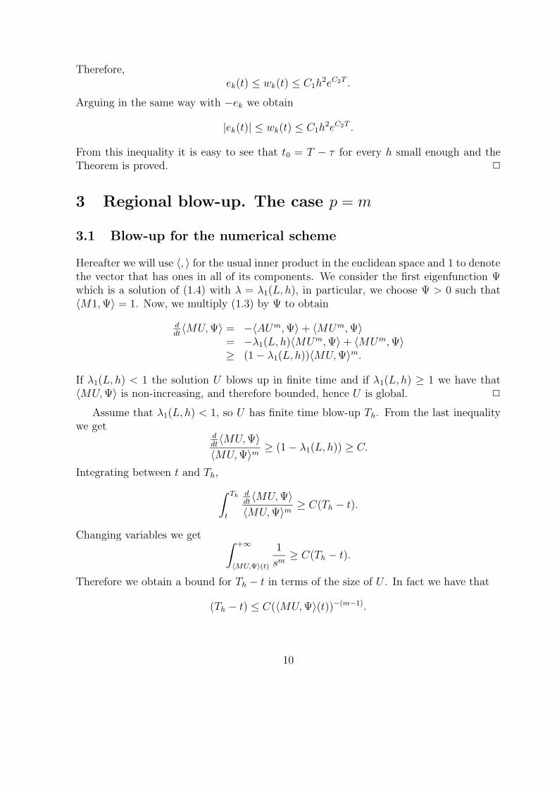
Assume that λ1(L, h) < 1, so U has finite time blow-up Th. From the last inequalitywe get
ddt〈MU,Ψ〉
〈MU,Ψ〉m≥ (1− λ1(L, h)) ≥ C.
Integrating between t and Th,
∫ Th
t
ddt〈MU,Ψ〉
〈MU,Ψ〉m≥ C(Th − t).
Changing variables we get∫ +∞
〈MU,Ψ〉(t)
1
sm≥ C(Th − t).
Therefore we obtain a bound for Th − t in terms of the size of U . In fact we have that
(Th − t) ≤ C(〈MU,Ψ〉(t))−(m−1).
10

This allows us to prove the convergence of the blow-up times. Given ε > 0 let R be suchthat CR−(m−1) ≤ ε/2. As blow-up for u is regional we can choose a time t0 such that
T − t0 ≤ ε/2 and
∫ L
−L
u(s, t0)ψ(s) ds ≥ 2R,
where ψ is the first eigenfunction of the laplacian in [−L,L]. By our uniform convergenceresult up to t = t0 < T , we have
〈MU,Ψ〉(t0) →
∫ L
−L
u(s, t0)ψ(s) ds, h→ 0.
Therefore for every h small enough, we have that
〈MU,Ψ〉(t0) > R.
Hence|T − Th| ≤ |T − t0|+ |Th − t0|
≤ ε/2 + C(〈MU,Ψ〉(t0))−(m−1)
≤ ε/2 + CR−(m−1)
≤ ε,
for every h small enough. This proves that Th → T as h→ 0.
3.2 Blow-up rate
From our previous computations we have that
〈MU,Ψ〉(t) ≤ C(Th − t)−1/(m−1).
Now we observe that there exists a constant C = C(h) such that
maxkuk(t) = u0(t) ≤ C〈MU,Ψ〉(t)
and we conclude thatu0(t) ≤ C(Th − t)−1/(m−1).
On the other hand, as for all t the solution is symmetric and decreasing in [0, L], we havethat
u′0(t) ≤ um0 (t).
Therefore, integrating between t and Th, we get
u0(t) ≥ C(Th − t)−1/(m−1).
Summing up, we have proved that the blow-up rate is given by
C1(Th − t)−1/(m−1) ≤ maxkuk(t) = u0(t) ≤ C2(Th − t)−1/(m−1).
11
3.3 Blow-up set
Theorem 3.1 If p = m every node is a blow-up point. Moreover in the self-similarvariables,
Y (s) → W, as s→∞,
where W = (w−N , ..., wN ) is a positive solution of the limit problem of (1.6). Hence theasymptotic behaviour of uk(t) is given by
uk(t) ∼ (Th − t)−1
p−1wk.
Proof. In this case, if we write the numerical problem (1.6) in a form similar to (1.2),we have a Lyapunov functional. In fact,
Φ(Y ) =1
2〈A1/2Y m, A1/2Y m〉+
1
2m〈MY m, Y m〉 −
1
m2 − 1〈MY m, Y 〉
satisfiesd
dsΦ(Y )(s) = −〈MY ′, Y m−1Y ′〉(s) ≤ 0.
Hence, the orbit Y (s) goes to a stationary state, see [H]. Therefore we study the limitproblem of (1.6). By Remark 2.1 we can restrict ourselves to [0, L] arriving to
0 =2
h2(wm
1 − wm0 )−
1
m− 1w0 + wm
0 ,
0 =1
h2(wm
k+1 − 2wmk + wm
k−1)−1
m− 1wk + wm
k , 0 ≤ k ≤ N − 1,
0 = wN .
(3.1)
Moreover, as we begin with a decreasing data U(0) then for a fixed s the vectorY (s) is positive and decreasing, hence we have to look to nonnegative and nondecreasingstationary solutions.
On the other hand, from the blow-up rate we know that y0(s) ≥ C(h) > 0, then W isnot the trivial solution. We claim that wk must be positive for all 0 < k < N . To provethis claim just suppose that there exists some j with wj = 0. Since W is non-negativeand non-increasing we have that for k ≥ j, wk = 0 and therefore wk = 0 for all k, butw0 > 0. This contradiction proves the claim. 2
Now our goal is to recover regional blow-up by looking carefully at the behaviour ofthe stationary solution as the parameter h goes to zero.
When h goes to zero we expect that Z = Wm converges to a solution of the followingproblem
zxx −1
m−1z
1
m + z = 0, x ∈ (0, L),
zx(0) = 0,z(L) = 0.
(3.2)
12

This is the content of our next Lemma. We remark that since m > 1 a non Lipschitzfunction appears in (3.2).
Lemma 3.1 Let W be the solution of (3.1) and let z(x) be the unique solution of (3.2).Then
Z = Wm → z(x), as h→ 0.
Proof. Multiplying the equation satisfied by Z by
(zk+1 − zk) + (zk − zk−1)
2
and summing we get
0 =(zN − zN−1)
2
2h2−
(z1 − z0)2
2h2+
N∑
l=1
(
zl −1
m− 1z
1
m
l
)
(zl+1 − zl−1)
2.
Hence
0 =(zN − zN−1)
2
2h2−
(z1 − z0)2
2h2
+
(
z2N
2−
m
m2 − 1z
(1+m)/mN
)
−
(
z20
2−
m
m2 − 1z
(1+m)/m0
)
+O(h).
Using the first and the last equations of (3.1) we get that zN−1 and z0 must verify thefollowing polynomial,
0 =z2
N−1
2h2−
m
m2 − 1z
1+mm
0 +z20
2+O(h). (3.3)
On the other hand, we know that z0 is bounded. Therefore, zN−1/h must be bounded.Then we can take a subsequence of h such that zN−1/h→ Γ ≥ 0.
If Γ > 0 we consider the auxiliary initial value problem
z′′ = 1m−1
z1/m − z, x ∈ [0, L],
z(L) = 0,z′(L) = −Γ.
(3.4)
For this problem we define the energy as
Ez(x) =(z′(x))2
2−
m
m2 − 1z(x)(m+1)/m +
z(x)2
2.
Multiplying equation (3.4) by z ′ and integrating we obtain that it is conservative, i.e.Ez(x) = Ez(L) = −Γ/2.
13

Problem (3.4) has a unique solution and by classical theory (see [JR]) in the intervalwhere z(x) is positive
Z = Wm → z(x), as h→ 0.
Notice that z(x) is positive in [L − δ, L). Since the vector Z is decreasing, we have thatz(x) is non-increasing in all interval [0, L]. Therefore z(x) is positive in [0, L). So, for allx ∈ [0, L), Z → z(x).
Then, as the problem is conservative and (3.3) holds, we get that z(0) is the onlypositive root of
Γ2
2−
m
m2 − 1z(0)(m+1)/m +
z(0)2
2= 0,
andz′(0) = 0.
So, the constant Γ must be the only constant such that z is a solution of
z′′ = 1m−1
z1/m − z, x ∈ [0, L],
z′(0) = 0,z(L) = 0,z(x) > 0, x ∈ [0, L).
This problem has a solution if and only if π2< L ≤ mπ
m−1, see the Appendix for the details.
So, if L > mπm−1
the parameter Γ must be zero.
Now, we assume that Γ = 0. Then Ez(L) = 0 and by (3.3) we obtain that z0 → A,where A is the only positive root of
0 =1
2A2 −
m
m2 − 1A
1+mm
and thatz′(0) = 0.
Hence, we consider the problem
z′′ = 1m−1
z1/m − z x ∈ [0, L],
z(0) = A,z′(0) = 0,z′(x) ≤ 0 x ∈ [0, L].
This problem has a unique explicit solution given by
z(x) =
{
[
2mm2−1
cos2(
(m−1)x2m
)]m
m−1
x < mπ/(m− 1),
0 x ≥ mπ/(m− 1).
Then if L < mπm−1
the parameter Γ must be positive.
14
On the other hand, by classical theory we have that in the interval where z(x) ispositive, [0,mπ/(m− 1)),
Z = Wm → z(x), as h→ 0.
Since Z is decreasing, we have that for h small enough,
zk ≤ z
(
mπ
m− 1− δ
)
≤ ε, ∀xk >mπ
m− 1− δ.
Then, Z = Wm → z(x) in all the interval [0, L]. 2
Remark 3.2 As a consequence of Lemma 3.1 if L > mπm−1
we have that
W → 0, in
[
mπ
m− 1, L
]
,
and we recover the regional blow-up in the sense that the constants that appear in theblow-up rate for the nodes that lie in [ mπ
m−1, L] go to zero as h goes to zero, i.e.,
uk(t) ∼ (Th − t)−1
p−1wk
with wk → 0 as h→ 0 for every k such that xk ∈ [ mπm−1
, L].
4 Single point blow-up. Case p > m.
4.1 Blow-up for the numerical scheme.
In this section we follow ideas from [GR]. We recall that we are considering a symmetricand decreasing in [0, L] initial data ϕ. By Lemmas 2.1 and 2.3 U(t) is a symmetric vectorand it is decreasing in [0, L]. Then, its maximum will be u0(t).
For the continuous problem (1.1) there exists an energy functional given by
Φ(u)(t) =1
2
∫ L
−L
(um)2x −
m
p+m
∫ L
−L
|u|p+m,
which is nonincreasing along the orbits. So let us define the discrete analogous of Φ, letΦh(U) be the following functional
Φh(U)(t) =1
2〈A1/2Um, A1/2Um〉 −
m
p+m〈MUp, Um〉,
which is also nonincreasing along the orbits.
15

Lemma 4.1 Let U be a solution such that Φh(U)(t0) < 0 for some t0, then U(t) isunbounded.
Proof. Let us assume that U is bounded, as Φh is a Lyapunov functional U(t) mustconverge to a steady state, W , as t goes to infinity. As Φh(U)(t0) < 0 and Φh is nonin-creasing, we get that Φh(W ) < 0. But, multiplying the equation satisfied by W by Wm
we get
0 = −〈A1/2Wm, A1/2Wm〉+ 〈MW p,Wm〉 = −2Φh(W ) +p+ 3m
p+m〈MW p,Wm〉.
Hence Φh(W ) ≥ 0, a contradiction. 2
Next, we prove that every solution with Φh(U)(t0) < 0 blows up.
Lemma 4.2 Let U be a solution such that Φh(U)(t0) < 0 for some t0 then U(t) blows upin finite time Th. Moreover, there exists a constant C independent of h such that
(Th − t0) ≤C
(−Φh(U(t0)))p−1
p+m
. (4.1)
Proof. From Lemma 4.1 we can assume that u0(t) = maxj uj(t) becomes unbounded.Therefore, using that p > m, we get
u′0(t) =1
h2(um
1 (t)− 2um0 (t) + um
−1(t)) + up0(t) ≥ δup
0(t),
for every t large enough. As p > m > 1 we obtain that u0 (and then U) blows up in finitetime.
On the other hand, we have that
ddt〈MU(t), Um(t)〉 = −(m+ 1)〈A1/2Um, A1/2Um〉(t) + (m+ 1)〈MU p, Um〉(t)
= −2(m+ 1)Φh(U(t)) +(m+ 1)(p−m)
(m+ p)〈MUp, Um〉(t)
≥ 2(m+ 1)|Φh(U(t))|+(m+ 1)(p−m)
(m+ p)〈MU,Um〉(m+p)/(m+1)(t)
≥ C (|Φh(U(t))|+ C〈MU,Um〉(t))(m+p)/(m+1) .
Now, integrating between t0 and Th and taking into account that Φh is non-increasing,we obtain the desired result. 2
We are ready to prove the following proposition, which completes the proof of Theo-rem 1.2.
16

Proposition 4.1 Let ϕ be such that u blows up in finite time then U , the solution of(1.3), also blows up for every h small enough.
First we observe that if u blows up in finite time T then
limt→T
Φ(u)(t) = −∞,
see [CDE].From our convergence result, it is easy to check that Φh(uh(·, t0)) → Φ(u(·, t0)) as
h → 0 and therefore we conclude that if u blows up in finite time then Φh(uh(·, t0)) < 0for some t0 and every h small enough, and hence uh blows up in finite time, Th.
To prove the convergence of the blow-up times we are going to use (4.1). We havethat, given ε > 0, we can choose R large enough to ensure that
(
C
Rp−1
p+m
)
≤ε
2.
As u blows up at time T we can choose t0 such that
T − t0 ≤ ε/2 and |Φ(u(·, t0))| ≥ 2R.
If h is small enough, by the convergence of Φh(uh(·, t0)) to Φ(u(·, t0)) we have,
|Φh(uh(·, t0))| ≥ R,
and hence, by (4.1),
Th − t0 ≤
(
C
(−Φh(U(t0)))p−1
p+m
)
≤
(
C
Rp−1
p+m
)
≤ε
2.
Therefore,
|Th−T | ≤ |Th−t0|+|T−t0| < ε. 2
4.2 Blow-up rate
Now we find the blow-up rate. Let us consider a blowing up solution U . Let us remarkthat by our symmetry assumptions u0(t) = maxj uj(t). Hence
up0(t) ≥ u′0(t) ≥ up
0
(
1−2
h2
um0
up0
)
(t).
Integrating we obtain
(Th − t) ≥
∫ Th
t
u′0up
0
(s) ds ≥
∫ Th
t
(
1−2
h2
um0
up0
)
(s) ds.
17

Therefore,
(Th − t) ≥1
(p− 1)up−10 (t)
≥
∫ Th
t
(
1−2
h2
um0
up0
)
(s) ds.
As u0(t) is blowing up and p > m we have that
limt↗Th
um0
up0
(t) = 0.
Hence we can conclude that,
limt↗Th
(Th − t)1/(p−1)u0(t) = Cp =
(
1
p− 1
)1
p−1
.
This implies that the blow-up rate is given by
C1
(Th − t)1/(p−1)≤ ‖U(t)‖∞ ≤
C2
(Th − t)1/(p−1).
Note that in this case the blow-up rate is independent of the parameter m.
4.3 Blow-up sets
Now we turn our interest to the blow-up set of the numerical solution. For a fixed h wewant to look at the set of nodes, xk, such that uk(t) → +∞ as t ↗ Th. As before, weintroduce the self-similar variables given by
yk(s) = (Th − t)1
p−1uk(t),
(Th − t) = e−s.
In these new variables Y = (yk(s)), problem (1.3) reads as (1.6). We observe that, fromthe blow-up rates proved in Theorem 1.3, the vector Y is bounded and
lims→∞
y0(s) = Cp > 0.
Theorem 4.1 If p > m, then U blows up at exactly K nodes near x = 0, i.e.
B(U) = [−Kh,Kh], K =
[
ln((p− 1)/(p−m))
ln(m)
]
Moreover, the asymptotic behaviour of the blowing up nodes is given by
u−j(t) = uj(t) ∼ (Th − t)γj , γj = −mj
p− 1+
j−1∑
l=0
ml,
18

ifln((p− 1)/(p−m))
ln(m)/∈ N or j 6= K, and by
u−K(t) = uK(t) ∼ − ln(Th − t), ifln((p− 1)/(p−m))
ln(m)∈ N.
Proof. First we want to prove that yj(s) → 0 for every j 6= 0, that is, the only nodethat behaves like Cp(Th − t)−1/(p−1) is x = 0. We argue by contradiction. Assume thatu1(t)(Th − t)1/(p−1) → Cp. Using that U is symmetric and decreasing in [0, L] we havethat
(u0 − u1)′(t) ≥
1
h2(3um
1 − 3um0 )(t) + (up
0 − up1)(t)
=
[
−3
h2
(
um0 − um
1
u0 − u1
)
+up
0 − up1
u0 − u1
]
(u0 − u1)(t)
=
[
−3
h2mξm−1 + pηp−1
]
(u0 − u1)(t),
where ξ and η lie between u1 and u0. As we have assumed that both u0 and u1 behavelike Cp(Th − t)−1/(p−1) we can conclude that
ξ(Th − t)1/(p−1) → Cp and η(Th − t)1/(p−1) → Cp.
As p > m we conclude that, for t near T ,
d
dtln(u0 − u1)(t) ≥
[
−3
h2mξm−1 + pηp−1
]
≥p(Cp−1
p − ε)
(Th − t).
Integrating we get(u0 − u1)(t) ≥ C(Th − t)−
p
p−1+pε.
Using this fact we have,
0 = limt→Th
(Th − t)1
p−1 (u0 − u1)(t) ≥ C limt→Th
(Th − t)1
p−1 (Th − t)−p
p−1+pε = +∞,
a contradiction that proves that (Th − t)1
p−1u1(t) → 0.
Now we return to the variable Y . From the blow-up rate for u0 we have that
lims→∞
y0(s) = Cp.
Now we observe that y1(s) verifies
y′1 = em−p
p−1s 1
h2(ym
0 − 2ym1 + ym
2 )−1
p− 1y1 + yp
1 ∼ Cem−p
p−1s −
1
p− 1y1
19

and by integration we get
0 ≤ y1(s) ∼
C e−p−m
p−1s p < m+ 1,
C s e−1
p−1s p = m+ 1,
C e−1
p−1s p > m+ 1.
Notice that in all cases y1(s) → 0. In the U variables, this translates into,
u1(t) ∼
C(Th − t)p−1−m
p−1 p < m+ 1,−C ln(Th − t) p = m+ 1,C p > m+ 1.
Therefore, if p ≤ 1 + m the node u1(t) blows up with a different rate than u0, and forp > m+ 1 it is bounded.
Repeating the argument for the other nodes we obtain that yk(s) → 0, for all k 6= 0.Moreover, the same calculations used before show how to obtain the asymptotic behaviourof each node using the behaviour of the previous one and the result follows. 2
5 Numerical experiments
In this Section we present some numerical experiments that illustrate our results. For thenumerical experiments we use the adaptive ODE solvers provided by MATLAB. In allcases we take L = 15 and the initial data ϕ(x) = L2 − x2 + 1.
First we deal with p = m = 1.5 and we find that the numerical blow-up time is givenby Th = 0.1382. Our numerical results are shown in figures 1 and 2. Figure 1 showsthe evolution of the numerical solution. Figure 2 shows the profile of the solution inself-similar variables near Th, we also put in the same picture the continuous self-similarprofile z(x). From this last picture one can appreciate that the numerical calculationsshow that the blow-up set is (−9.4248, 9.4248) ≈ (−3π, 3π).
Finally, we consider the case p = 2, m = 1.5. In this case, Th = 0.004432. In Figure3 one can see the evolution of the solution. In order to obtain the numerical blow-uprates, in Figure 4 we display ln(ui) versus − ln(Th − t) for i = 0, 1, 2. We can appreciatethat the first curve (corresponding to max uk = u0) has slope 1, the second (for u1) hasslope 1/2 (it becomes parallel to the dotted line which has slope 1/2) and the last one(for u2) is flat. These behaviours correspond to the expected rates u0(t) ∼ (Th − t)−1,u1(t) ∼ (Th − t)−1/2 and u2 bounded.
20

0
4
8
x 1010
�
���
�
�
Figure 1. Evolution of the numerical solution (p = m).
−15 −10 −5 0 5 10 150
1
2
3
4
5
6
����� �
��� �����
Figure 2. Self-similar profiles (p = m).
21

0
0.5
1
1.5
2
2.5
3
3.5
4
4.5
x 105
�
���
��
Figure 3. Evolution of the numerical solution (p > m).
6 8 10 12 14 16 18 20 22 24 26 28
6
8
10
12
14
16
18
20
22
24
26
28
��� ���� ������
� � ������������� ��������� � �!� �����"��
Figure 4. Blow-up rates (p > m).
22

6 Appendix
In this appendix we search for nonnegative monotone solutions of the following boundaryvalue problem
{
(fm)′′ = 1m−1
f − fm, x ∈ [0, L],
f ′(0) = 0, f(L) = 0,(6.1)
We note that if f(x) is a solution of this problem then
u(x, t) = (T − t)−1/(m−1)f(x)
is a solution of
ut = (um)xx + um, (x, t) ∈ (0, L)× [0, T ),(um)x(0, t) = 0, t ∈ [0, T ),u(L, t) = 0, t ∈ [0, T ),u(0, t) = T−1/(m−1)f(x).
This problem has been studied in [SGKM] and we know that for all positive initial data(i) u(x, t) blows up if and only if L > π/2.(ii) The blow rate is given by ‖u(x, t)‖∞ ∼ (T − t)−1/(m−1).On the other hand, following a standard technique we introduce the self similar vari-
ablesv(x, τ) = (T − t)
1
m−1u(x, t), τ = − ln(T − t).
This function v(x, τ) satisfies the following problem,
vτ = (vm)xx −1
m−1v + vm, (x, τ) ∈ (0, L)× (0,+∞),
(vm)x(0, τ) = 0, τ ∈ (0,+∞),v(L, τ) = 0, τ ∈ (0,+∞),
v(x, 0) = T1
m−1u(x, 0), x ∈ (0, L).
(6.2)
We remark that the stationary solutions of (6.2) are solutions of (6.1).
Now, we prove that v(x, τ) converges (in terms of ω-limits) to a stationary state. Forthis we multiply the equation by (vm)τ and integrate with respect to x to obtain
∫ L
0
(vm)τvτ = −d
dtF (v),
where
F (v) =
∫ L
0
(vm)2x
2(s, τ) ds+
m
m2 − 1
∫ L
0
vm+1(s, τ) ds−1
2
∫ L
0
v2m(s, τ) ds.
Hence F (v) is a Lyapunov functional for problem (6.2) and we can conclude that theω−limit set of v(x, τ) consists of nontrivial stationary solutions of (6.2).
23

Lemma 6.1 Let f(x) be a solution of (6.1). Then,(i) if L ≤ π/2 no solution exists,(ii) if π/2 < L < (mπ)/(m− 1) there exists a unique positive solution and(iii) if L ≥ (mπ)/(m− 1) the unique monotone solution is given by
f(x) =
[
2mm2−1
cos2(
(m−1)x2m
)]1
m−1
x < mπ/(m− 1),
0 x ≥ mπ/(m− 1).
Proof. From the previous argument we have that problem (6.1) has a solution if andonly if L > π/2.
In order to prove the uniqueness we consider two different solutions of (6.1), f1(x)and f2(x) . These profiles must have some intersections. If this is not the case, they areordered and hence the corresponding solutions in variables (x, t) do not have the sameblow-up time. Since the energy
Ef (x) =(f ′(x))2
2−
m
m2 − 1f(x)(m+1)/m +
f(x)2
2
is a nonnegative constant function, we obtain that two different profiles have only oneintersection point. Moreover, f ′1(L) < f ′2(L) ≤ 0 if and only if f1(0) > f2(0), which is acontradiction with the fact that they have only one intersection point. Finally we remarkthat, as the energy must be nonnegative, we have
f(0) ≥ A =
(
2m
m2 − 1
)1
m−1
,
and for each f(0) ≥ A there exists a unique L ∈ (π/2, (mπ)/(m − 1)] such that f(x)is a positive solution of (6.1). For L > (mπ)/(m − 1) we extend by zero for all x ∈[(mπ)/(m− 1), L]. 2
Acknowledgements
We want to thank B. Ayuso and J. P. Moreno for several interesting discussions. Alsowe want to thank J. L. Vazquez for his encouragement and valuable suggestions.
References
[ALM1] L. M. Abia, J. C. Lopez-Marcos, J. Martinez. Blow-up for semidiscretizationsof reaction diffusion equations. Appl. Numer. Math. Vol. 20, (1996), 145-156.
[ALM2] L. M. Abia, J. C. Lopez-Marcos, J. Martinez. On the blow-up time convergenceof semidiscretizations of reaction diffusion equations. Appl. Numer. Math. Vol.26, (1998), 399-414.
24

[BB] C. Bandle and H. Brunner. Blow-up in diffusion equations: a survey. J. Comp.Appl. Math. Vol. 97, (1998), 3-22.
[BK] M. Berger and R. V. Kohn. A rescaling algorithm for the numerical calculationof blowing up solutions. Comm. Pure Appl. Math. Vol. 41, (1988), 841-863.
[BHR] C. J. Budd, W. Huang and R. D. Russell. Moving mesh methods for problemswith blow-up. SIAM Jour. Sci. Comput. Vol. 17(2), (1996), 305-327.
[Ch] Y. G. Chen. Asymptotic behaviours of blowing-up solutions for finite differenceanalogue of ut = uxx + u1+α. J. Fac. Sci. Univ. Tokyo Sect. IA Math. Vol. 33(3), (1986), 541–574.
[Ci] P. Ciarlet. The finite element method for elliptic problems. North Holland,(1978).
[CDE] C. Cortazar, M. del Pino and M. Elgueta. The problem of uniqueness of thelimit in a semilinear heat equation. Comm. Partial Differential Equations.Vol. 24(11&12), (1999), 2147-2172.
[DER] R. G. Duran, J. I. Etcheverry and J. D. Rossi. Numerical approximation of aparabolic problem with a nonlinear boundary condition. Discr. and Cont. Dyn.Sys. Vol. 4 (3), (1998), 497-506.
[FBR] J. Fernandez Bonder and J. D. Rossi. Blow-up vs. spurious steady solutions.Proc. Amer. Math. Soc. Vol. 129 (1), (2001), 139-144.
[FG] R. Fletcher and D. F. Griffiths. The generalized eigenvalue problem for certainunsymmetric band matrices. Linear Algebra Appl., Vol. 29, (1980), 139–149.
[GR] P. Groisman and J. D. Rossi. Asymptotic behaviour for a numerical approxima-tion of a parabolic problem with blowing up solutions. J. Comput. Appl. Math.Vol. 135 (1), (2001), 135–155.
[H] Henry. Geometric theory of semilinear parabolic equation. Lecture Notes inMath. Vol. 840. Springer Verlag, (1981).
[JR] L. W. Johnson and R. D. Riess. Numerical analysis. Addison-Wesley, (1982).
[LSU] O. A. Ladyzhenskaya, V. A. Solonnikov, N. N. Ural’tseva, Linear and quasilinearequations of parabolic type, Transl. Math. Monographs Vol. 23. Amer. Math.Soc., Providence, 1968.
[L] H. A. Levine. The role of critical exponents in blow up theorems. SIAM Rev.Vol. 32, (1990), 262–288.
25

[LR] M.N Le Roux. Numerical solution of fast diffusion or slow diffusion equations.J. Comput. Appl. Math. Vol. 97 (1-2), (1998), 121–136.
[N] T. Nakagawa. Blowing up of a finite difference solution to ut = uxx +u2.. Appl.Math. Optim. Vol 2 (4), (1975/76), 337–350.
[NU] T. Nakagawa and T. Ushijima. Finite element analysis of semilinear heat equa-tion of blow-up type, in: Topics in numerical analysis. III (J.H. Miller, ed.).Academic Press, London (1977) 275–291.
[P] C. V. Pao, “Nonlinear parabolic and elliptic equations”. Plenum Press, NewYork, (1992).
[SGKM] A. A. Samarskii, V. A. Galaktionov, S. P. Kurdyumov and A. P. Mikhailov.“Blow-up in problems for quasilinear parabolic equations”. Nauka, Moscow,(1987) (in Russian). English transl.: Walter de Gruyter, Berlin, (1995).
26