numerical analysis of phase change material for...

NUMERICAL ANALYSIS OF PHASE CHANGE MATERIAL FOR

ENERGY STORAGE SYSTEM

WAN KHAIRUL MUZAMMIL B ABDUL RAHIM

FACULTY OF ENGINEERING UNIVERSITY OF MALAYA

KUALA LUMPUR

2012

NUMERICAL ANALYSIS OF PHASE CHANGE MATERIAL FOR

ENERGY STORAGE SYSTEM

WAN KHAIRUL MUZAMMIL B ABDUL RAHIM

RESEARCH REPORT SUBMITTED IN PARTIAL FULFILMENT OF THE REQUIREMENT FOR DEGREE OF MASTER OF

ENGINEERING

FACULTY OF ENGINEERING UNIVERSITY OF MALAYA

KUALA LUMPUR

2012

UNIVERSITI MALAYA

ORIGINAL LITERARY WORK DECLARATION

Name of Candidate: (I.C/Passport No: )

Registration/Matric No:

Name of Degree:

Title of Project Paper/Research Report/Dissertation/Thesis (“this Work”):

Field of Study:

I do solemnly and sincerely declare that:

(1) I am the sole author/writer of this Work; (2) This Work is original; (3) Any use of any work in which copyright exists was done by way of fair dealing and for

permitted purposes and any excerpt or extract from, or reference to or reproduction of any copyright work has been disclosed expressly and sufficiently and the title of the Work and its authorship have been acknowledged in this Work;

(4) I do not have any actual knowledge nor do I ought reasonably to know that the making of this work constitutes an infringement of any copyright work;

(5) I hereby assign all and every rights in the copyright to this Work to the University of Malaya (“UM”), who henceforth shall be owner of the copyright in this Work and that any reproduction or use in any form or by any means whatsoever is prohibited without the written consent of UM having been first had and obtained;

(6) I am fully aware that if in the course of making this Work I have infringed any copyright whether intentionally or otherwise, I may be subject to legal action or any other action as may be determined by UM.

Candidate’s Signature Date

Subscribed and solemnly declared before,

Witness’s Signature Date

Name: Designation:

WAN KHAIRUL MUZAMMILB ABD RAHIM

KGH100032

M.Eng. MECHANICAL ENGINEERING

NUMERICAL ANALYSIS OF PHASE CHANGE MATERIALFOR ENERGY STORAGE SYSTEM

ENERGY

iii

ACKNOWLEDGEMENT

I hereby would like to express my utmost gratitude towards my supervisor and mentor;

Prof. Dr. T.M.I. Mahlia for his continuous guidance, motivation, patience and help during

the entire period of this research report was written. To my dearly loved wife, for her

constant inspiration, encouragement and strength which helps me to cope with all the

challenges during my course of study. And to my beloved parents and sisters, anchors of

my life; thank you for giving me the courage to face the unknown.

iv

ABSTRACT

A numerical method based on the effective heat capacity method was studied to solve the

phase change heat transfer problems of a phase change material in a cylindrical latent heat

thermal energy storage device during the charging (melting) process of the material. The

commercial software COMSOL Multiphysics was employed to run the numerical

simulations. The effective heat capacity method was used to characterize the fusion heat of

melting of the phase change material and the moving boundary of solid-liquid interface. An

analytical tool was used to validate the phase change heat transfer process in which the

results show a good agreement between the numerical and analytical analysis.

Subsequently, the effects of fins and various heat transfer velocities on the thermal behavior

of the PCM were studied numerically using the software. Generally, the results obtained

from the analysis show that the heat transfer rate increases as the number of fins and HTF

velocities were increased. For small number of fins configurations, the effect of increasing

the HTF velocities are not so significant, as the thermal resistance of the phase change

material is high. However, the effect is more evident as the number of fins increases; due to

the decreasing thermal resistance on the PCM side.

v

ABSTRAK

Suatu kaedah berangka berdasarkan kaedah muatan haba berkesan telah dikaji untuk

menyelesaikan masalah pemindahan haba bagi suatu bahan ubah fasa di dalam alat

penyimpan tenaga haba pendam berbentuk silinder semasa proses pelakuran bahan tersebut.

Perisian komersial COMSOL Multiphysics telah digunakan untuk menjalankan simulasi

berangka berdasarkan kaedah muatan haba berkesan. Kaedah tersebut digunakan untuk

menggambarkan ciri-ciri pelakuran bahan ubah fasa dan pergerakan sempadan antara fasa-

fasa pepejal dan cecair. Analisa ke atas bahan ubah fasa telah dilakukan untuk

pengesahsahihan proses ubah fasa. Pengiraan yang dibuat telah menunjukkan hasil yang

baik antara kaedah berangka dan kaedah analisa yang digunakan. Seterusnya, suatu ujikaji

ke atas kesan penambahan sirip dan pengunaan bendalir pindah haba berlainan halaju telah

dilakukan menggunakan perisian COMSOL. Secara amnya, hasil daripada ujikaji yang

dijalankan menunjukkan bahawa kadar pemindahan haba meningkat dengan bertambahnya

jumlah bilangan sirip dan peningkatan halaju bendalir pindah haba di dalam alat penyimpan

tenaga haba pendam tersebut. Bagi jumlah konfigurasi sirip yang kecil, kesan peningkatan

halaju bendalir pindah haba adalah tidak signifikan kerana rintangan terma di dalam bahan

ubah fasa adalah tinggi. Walaubagaimanapun, rintangan terma itu berkurangan apabila

jumlah sirip bertambah.

vi

Table of Contents Declaration ii

Acknowledgement iii

Abstract iv

Abstrak v

Table of Contents vi

List of Tables vii

List of Figures ix

List of Symbols and Abbreviations xiii

CHAPTER 1 - INTRODUCTION

1.1 Background of study 1

1.2 Statement of problem 2

1.3 Objectives of study 3

1.4 Research scope 4

1.5 Research methodology 4

1.6 Organization of research report 5

CHAPTER 2 - LITERATURE REVIEW

2.1 Thermal energy storage systems 7

2.1.1 Sensible heat energy storage 8

2.1.2 Thermochemical heat energy 9

2.1.3 Latent heat energy storage 10

2.2 Phase change materials used in latent heat energy storage 11

2.2.1 Desirable properties of phase change materials 11

2.2.2 Classification of PCMs 13

2.3 Geometry of thermal energy storage systems 18

2.3.1 Rectangular geometry 18

2.3.2 Spherical geometry

2.3.3 Cylindrical geometry

2.3.4 Finned geometry

19

20

22

2.4 Heat transfer in phase change materials 24

2.4.1 Stefan problem 24

2.4.2 Solving the Stefan problem 25

CHAPTER 3 - METHODOLOGY: GEOMETRICAL DESIGN AND GOVERNING MATHEMATICAL EQUATIONS

3.1 Latent heat thermal energy storage device geometrical arrangement,

dimensions and materials

29

3.1.1 Selection of fins 31

3.2 Heat transfer, fluid flow and phase change processes 32

3.2.1 Heat transfer process 32

vii

3.2.2 Fluid flow process 34

3.2.3 Phase change heat transfer process 35

3.3 Numerical analysis 36

3.3.1 Numerical model 36

CHAPTER 4 - VALIDATION OF PHASE CHANGE PROCESS

4.1 Analytical study 43

4.2 Numerical study 47

4.3 Validation 52

CHAPTER 5 - LATENT HEAT THERMAL ENERGY STORAGE:

NUMERICAL ANALYSIS RESULTS AND DISCUSSION

5.1 Numerical analysis - mesh convergence study 55

5.2 Energy stored in LHTES: Integrating COMSOL functions 59

5.3 Effects of HTF velocities 60

5.4 Effects of number of fins as thermal enhancers 74

5.4.1 Effects of the addition of fins at HTF velocity of 0.01 m/s 74

5.4.2 Effects of the addition of fins at HTF velocity of 0.1 m/s 78

5.5 LHTES maximum storage capacity and efficiency 81

CHAPTER 6 - CONCLUSION

6.1 Conclusion 85

6.2 Recommendations 87

REFERENCES 88

APPENDIX A 94

APPENDIX B 102

APPENDIX C 104

viii

List of Tables

TABLE PAGE

2.1 Studies on finned geometry of thermal energy storage devices 23

3.1 Latent heat thermal energy storage device dimensions and materials 29

3.2 Properties of the materials used 30

4.1 Various mesh element sizes used for the simulation 48

5.1 Boundary and initial conditions used in the convergence study 56

5.2 Various element sizes used in the convergence study and their data 57

5.3 Sensible energy percentage increase in the LHTES for various

numbers of fins as the HTF velocity increases from 0.01 m/s to 0.1

m/s.

68

5.4 Latent energy percentage increase in the LHTES for various numbers

of fins as the HTF velocity increases from 0.01 m/s to 0.1 m/s

70

5.5 Total energy percentage increase in the LHTES for various numbers

of fins as the HTF velocity increases from 0.01 m/s to 0.1 m/s

71

ix

List of Figures

FIGURE PAGE

1.1 Schematic diagram of a solar water heater system with LHTES 3

2.1 Various types of thermal energy storage 8

2.2 Classification of phase change materials 13

3.1 Front and top side drawings of the LHTES with single fin

configuration

30

3.2 Geometrical representations of 0, 1, 3 and 7 fins configuration of

LHTES

31

3.3 The modified heat capacity of the paraffin wax defined from

temperature range of 290 K to 350 K

41

4.1 One-dimensional analytical moving boundary phase change problem 44

4.2 Schematic diagram of the 2D slab of paraffin wax 48

4.3 Simulated 2D surface temperature plot. Simulated time: 21 hours 49

4.4 Temperature distribution profile along section P-P for various mesh

element sizes. Simulated time: 3 hours

50

4.5 Temperature history of points A, B C and D. Simulated time: 18 hours 51

4.6 Temperature distribution profile for various simulated time 52

4.7 Comparison of numerical and analytical temperature distribution

profiles for various simulated times

52

4.8 Melting front position obtained from numerical and analytical studies.

Simulated time: 12 hours

53

5.1 A meshed axisymmetric 2D model of the LHTES used in the

numerical studies. The outer surfaces of the model are thermally

insulated

56

5.2 A 12 fins configuration LHTES with its 2D surface temperature plot

used in the convergence study. Simulated time: 21 hours.

57

5.3 Temperature profile plots for various mesh element sizes at line P-P.


58

5.4 Temperature distribution plots for the 7 fins configuration LHTES

with various HTF velocities and their Reynolds numbers. Simulated

time: 12 hours

61

5.5 Temperature distribution plots for the 15 fins configuration LHTES

with various HTF velocities and their Reynolds numbers. Simulated

time: 12 hours

62

5.6 Slow heating zone (SHZ) between the fins and the enclosure reduces

the melting fraction of the PCM

63

5.7 Total energy stored for the 0 fin configuration LHTES over 12 hours

of simulated time for various HTF velocities

64

5.8 Total energy stored for the 1 fin configuration LHTES over 12 hours


65

x

5.9 Total energy stored for the 6 fins configuration LHTES over 12 hours


65

5.10 Total energy stored for the 7 fins configuration LHTES over 12 hours


66

5.11 Total energy stored for the 12 fins configuration LHTES over 12

hours of simulated time for various HTF velocities

66



67



67



68

5.15 Sensible thermal energy stored in various numbers of fins

configuration for HTF velocities of 0.01 m/s, 0.03 m/s, 0.05 m/s and

0.1 m/s. Simulated time: 12 hours

69

5.16 Latent thermal energy stored in various numbers of fins configuration

for HTF velocities of 0.01 m/s, 0.03 m/s, 0.05 m/s and 0.1 m/s.


70

5.17 Total thermal energy stored in various numbers of fins configuration

for HTF velocities of 0.01 m/s, 0.03 m/s, 0.05 m/s and 0.1 m/s.


72

5.18 Melting fraction for various HTF velocities from 0 to 24 fins

configuration. Simulated time: 12 hours

73

5.19 Temperature distribution plots for the 1, 6, 12, 18 and 24 fins

configuration after 12 hours of simulated charging time. U0= 0.01 m/s

75

5.20 Total energy stored in 0 to 24 fins configuration of the LHTES after

12 hours of simulated charging time. U0 = 0.01 m/s

76

5.21 Sensible and latent thermal energy stored in 0 to 24 fins configuration

after 12 hours of simulated charging time. U0 = 0.01 m/s.

77

5.22 Temperature distribution plots for the 1, 6, 12, 18 and 24 fins

configuration after 12 hours of simulated charging time. U0= 0.1 m/s

78

5.23 Total energy stored in 0 to 24 fins configuration of the LHTES after

12 hours of simulated charging time. U0 = 0.1 m/s

79

5.24 Sensible and latent thermal energy stored in 0 to 24 fins configuration

after 12 hours of simulated charging time. U0 = 0.1 m/s

80

5.25 Total energy stored for various HTF velocities as compared to the

maximum storage capacity for 0 to 24 fins configuration of LHTES

after simulated charging time of 12 hours

82

5.26 Thermal energy storage efficiencies for various numbers of fins after

12 hours of simulated charging time. HTF velocities: 0.01 m/s and 0.1

m/s

83

A.1 Temperature distribution plots for 0 fin configuration LHTES with 94

xi

various HTF velocities and their Reynolds numbers. Simulated time:

12 hours

A.2 Temperature distribution plots for 1 fin configuration LHTES with


12 hours

95

A.3 Temperature distribution plots for 2 fins configuration LHTES with


12 hours

95



12 hours

96



12 hours

96



12 hours

97



12 hours

97



12 hours

98



12 hours

98



12 hours

99



12 hours

99



12 hours

100



12 hours

100



12 hours

101

xii

B.1 Temperature distribution plots for the 0, 1, 2, 3 and 4 fins

configuration LHTES after 12 hours of simulated charging time.

u0=0.01 m/s

102

B.2 Temperature distribution plots for the 5, 6, 7, 9 and 12 fins


u0=0.01 m/s

103

B.3 Temperature distribution plots for the 15, 18, 21 and 24 fins


u0=0.01 m/s

103

C.1 Temperature distribution plots for the 0, 1, 2, 3 and 4 fins


u0=0.1 m/s

104

C.2 Temperature distribution plots for the 5, 6, 7, 9 and 12 fins


u0=0.1 m/s

105

C.3 Temperature distribution plots for the 15, 18, 21 and 24 fins


u0=0.1 m/s

105

xiii

List of Symbols and Abbreviations

SYMBOL

Cap Average specific heat between Ti and Tf (J/kg.K)

Ck Specific heat of phase k in PCM (J/kg.K)

Cp Specific heat (J/kg.K)

��,�� Effective heat capacity (J/kg.K)

��,� Liquid PCM specific heat (J/kg.K)

��,�� Modified heat capacity (J/kg.K)

��,� Solid PCM specific heat (J/kg.K)

Clp Average specific heat between Tm and Tf (J/kg.K)

Csp Average specific heat between Ti and Tm (J/kg.K)

f Melt fraction

��2ℎ� COMSOL function

g Acceleration of gravity (m/s2)

H Total volumetric enthalpy (J/m3)

h Sensible volumetric enthalpy (J/m3)

ℎ� Prescribed function of � > 0

∆ℎ� Heat of fusion per unit mass (J/kg)

∆ℎ� Endothermic heat of reaction

k Thermal conductivity (W/m.K)

kk Thermal conductivity of phase k in PCM (J/kg.K)

L Latent heat of fusion (J/kg)

m Mass (kg)

��⃗ Normal to

P Pressure (Pa)

Q Energy stored (J)

q Heat flux (W/m2)

R,r Cylindrical coordinate (m)

r Radius (m)

S(t) Location of solid-liquid interface as a function of time (m)

Ste Stefan number

T Temperature (K)

t Time (s)

u Velocity (m/s)

X,x Space coordinate (m)

Z,z Space coordinate (m)

xiv

GREEK LETTERS

� Thermal diffusivity of PCM (m2/s)

�� Fraction melted

�� Fraction reacted

� Constant

� Similarity variable

� Angle (°)

� Density (kg/m3)

� Dynamic viscosity (N.s/m2)

� Kinematic viscosity (m2/s)

� Viscous dissipation (m2/s2)

SUBSCRIPT

f Final

� Initial

in Inlet

� Liquid

� Melting

r In the radial direction

� Solid

� Wall

GENERAL

DOF Degree of freedom

FEM Finite element method

HTF Heat transfer fluid

LHTES Latent heat thermal energy storage

PCM Phase change material

SHS Sensible heat storage

SHZ Slow Heating Zone TES Thermal energy storage

1

CHAPTER 1

INTRODUCTION

1.1 Background of study

In the interest of reducing energy usage in a wide variety of industrial and commercial

applications, many efforts have been initiated to utilize renewable energy sources and to

enhance the usage of waste energy. One way to solve the issue of wasted energy is by

storing the excess energy into thermal energy storage (TES) which would increase the

efficiency of energy consumption and production. TES can be categorized as sensible,

latent, or the combination of these two types of heat systems. Between these two types of

thermal energy storage systems; latent heat thermal energy storage (LHTES) system is a

more attractive technology due to its higher density of energy storage capabilities.

Furthermore, as comparison to the conventional sensible heat thermal energy storage

system, LHTES system has smaller volume and less weight for a given amount of energy

stored.

Latent heat storage using phase change materials (PCMs) have been gaining much attention

over the last few decades due to its capability to store heat of fusion at a constant or near

constant temperature which corresponds to the solid-liquid phase change material. During

the charging (or melting) process, the thermal energy is stored in phase change materials,

and recovered during the discharging (or freezing) process (Zalba et al., 2003, Sharma et

al., 2009, Benli and Durmus, 2009). Various industrial, commercial and laboratorial

2

applications have adopted the use of latent heat thermal energy storage system such as in

solar energy heating system (Saman et al., 2005, Shukla et al., 2009, Hasnain, 1998), waste

heat recovery (Azpiazu et al., 2003, Go et al., 2004) and conservation of energy in building

(Kuznik et al., 2008, Tyagi and Buddhi, 2007, Liu and Chung, 2005).

For the current study, the latent heat thermal energy storage can be applied in a solar hot

water system application as shown in Fig. 1.1. When solar energy is available, the cold

heat transfer fluid (HTF) is pumped to the solar collector whilst the isolation valve

connecting the hot and cold pipes is closed. The high temperature fluid from the solar

collector then flows through the latent heat thermal energy storage device and melts

(charging process) the PCM inside. The high temperature fluid continues to flow into the

water tank, heating the cold water supply. At night, when there is no solar energy available

the valves leading to and from the solar collector are closed, and the isolation valve

between the hot and cold pipes is opened; creating a shorter route for the HTF. The

discharging process occurs where the thermal energy from the PCM is transferred to the

HTF, increasing its temperature and then flows into the water tank. The

discharging/solidification process however is not included in the scope of research. On the

other hand, the focus of the study is to investigate the effects of fins and HTF velocities on

the thermal behavior of the PCM in the LHTES device.

1.2 Statement of problem

For this study, an investigation of a phase change material; namely paraffin wax is used in a

cylindrical latent heat thermal energy storage device to analyze the effects of fins in the

system and the velocities of heat transfer fluids on the melting of PCM.

3

Fig. 1.1. Schematic diagram of a solar water heater system with LHTES.

1.3 Objectives of study

The objectives of this research study are as follows:-

1. To study a method of numerical analysis pertaining to phase change heat transfer

problems in a cylindrical latent heat thermal energy storage device during the

charging process through the use of commercial software COMSOL Multiphysics.

2. To investigate the effects of thermal enhancers or fins in cylindrical latent heat

thermal energy storage device as well as the effects of heat transfer fluid velocities

on the thermal behavior of phase change material.

4

1.4 Research scope

The scope of this study mainly focuses on the effects of the addition of fins and heat

transfer velocities on the thermal behavior of the phase change material. The geometry of

the thermal storage device is translated into the COMSOL software where various

mathematical equations and boundary conditions are solved numerically through the use of

finite element analysis method in the software. Validation on the numerical study results of

the phase change process (Stefans problem) for a semi-infinite slab is carried out using

analytical tool. Afterwards, study on the effects of fins and the velocities of the thermal

fluid are presented in the subsequent chapters where the latent heat thermal energy storage

system numerical results are summarized and discussed.

1.5 Research methodology

The research methodology can be simply explained with the following steps:

Step 1: Selection of geometry, fins and dimensions of the LHTES.

Step 2: Translate the desired geometry into COMSOL Multiphysics.

Step 3: Materials for the system are assigned to its individual parts.

Step 4: Meshing of the geometry.

Step 5: Carry out the finite element analysis through the use of COMSOL.

Step 6: Extract the relevant data and discuss.

Step 7: Present the conclusions of the study.

5

1.6 Organization of research report

Chapter 1

This chapter consists of a background of study of the research project. Furthermore, a

simple discussion on an overview of the project methodology is presented as well as the

outline of the study.

Chapter 2

The second chapter consists of literature review on the study of the latent heat thermal

energy storage where various geometries used in recent researches are presented as well as

discussion on different phase change materials.

Chapter 3

This chapter includes the discussions on the geometrical arrangement, dimensions and the

materials used for the numerical studies on the LHTES device. Also in this chapter, the

governing physical equations and mathematical formulations used in the study are

presented.

Chapter 4

The fourth chapter describes about an analytical validation of the numerical results data

obtained from the simulation of heating a semi-infinite paraffin slab.

Chapter 5

The results and discussion obtained from the numerical study of an axisymmetric 2D latent

heat thermal energy storage is presented in the fifth chapter.

6

Chapter 6

This chapter concludes the main findings of the research report.

7

CHAPTER 2

LITERATURE REVIEW

2.1 Thermal energy storage systems

Renewable energy has become one of the most important topics recently which has seen

various developments and critical breakthroughs in technological advancement in order to

optimize the use of energy more efficiently. The high level of greenhouse gas emissions

and the ever increasing of fuel prices played a major and yet destructive role to realize the

importance of utilizing energy as efficient as possible to reduce the waste of energy into the

environment. There are many new and renewable energy methods that can be utilized to

extract energy from the wasted or exhausted energy sources. Energy storage devices are

one of the most widely used technique that can be implemented in most industrial and

commercial applications. The disparity between demand and supply can be reduced through

the use of energy storage. Furthermore, the reliability and performance of energy systems

can be enhanced which can be an advantage to conserve the energy used (Garg et al.,

1985).

In the past few decades, the use of phase change materials to store thermal energy has been

used in many researches due to its great prospect and commercial values (Dutil et al., 2011,

Agyenim et al., 2010, Sharma et al., 2009, Nayak et al., 2006, Anica, 2005, Rosen and

Dincer, 2003). Thermal energy storage systems can be used to collect energy at a certain

period and deliver it in a later time, increase the efficiency of a refrigerator (Cheng et al.,

8

2011) or to provide output stability for any plants in areas with cloudy weather conditions.

The types of thermal energy storage can be classified by the different forms of the change

in internal energy of the materials used in the devices. A summary of the different types of

thermal energy storage is illustrated in Fig. 2.1 (Baylin, 1979).

Fig. 2.1. Various types of thermal energy storage.

2.1.1 Sensible heat energy storage

Sensible heat storage (SHS) involves the storing of energy by raising the temperature of a

medium (solid or liquid) with high heat capacity. The storage medium can be water, bricks,

sand, rock beds, oil or soil. Together with a container, and input/output device is attached to

it to provide thermal energy for any intended application. Most commonly used in

dwellings, SHS is used as heat storage to provide hot water for houses and offices. The

system depends heavily on the heat capacity and the change in the temperature of the

Thermal Energy Storage

Thermal

Sensible Heat

Liquids Solids

Latent Heat

Solid-liquid Liquid-gaseous Solid-solid

Chemical

9

medium during the charging and discharging process. Furthermore, the amount of total

energy that can be stored in the system depends on the specific heat of the medium, the

volume of the material used and the temperature change (Lane, 1983). Hence, the total

energy stored in a sensible heat energy storage system can be calculated by using the

following equation:

� = ∫ ��

� = ��(�� − ��)

Where �� and �� denote the final and initial temperatures; whereas �� denotes the average

specific heat between the initial and final temperatures. However, SHS systems have a few

disadvantages. There are: (i) Non-isothermal behavior during charging (storing of heat) and

discharging (releasing of heat) processes, and (ii) Low heat storage capacity per unit

volume of the medium.

2.1.2 Thermochemical heat energy storage

In thermochemical energy storage system, the energy is stored after a breaking or

dissociation reaction of chemical bonds at molecular level which releases energy and then

recovered in a completely reversible chemical reaction. The thermochemical energy storage

system process can be illustrated by the following equation which describes the amount of

heat that can be stored is directly dependent on the amount of storage material, the extent of

conversion and the endothermic heat of reaction (Sharma et al., 2009):

� = ��∆ℎ�

(2.1)

(2.2)

(2.3)

10

where ∆ℎ� is the endothermic heat of reaction, � is the mass of heat storage medium and

�� is the fraction reacted. To date, thermochemical heat energy storage has not yet been

used in practical applications due to a few economical and technical aspects that needed to

be improved before it becomes viable (Agyenim et al., 2010).

2.1.3 Latent heat energy storage

Latent heat storage system is based on the high latent heat of a phase change material which

stores the released energy through the phase change process of the storage medium that

occurs at specific temperature range. The phase change process can either be from solid to

liquid, liquid to gas or vice versa. The storage capacity of any latent heat energy storage

system is given by (Lane, 1983):

� = ∫ ��d� +��∆ℎ� + ∫ ��d��

��

��

� = ��(�� − ��) + ��∆ℎ� + ��(�� − ��)�

Where Tm denotes the melting temperature, am is the melted fraction, ∆ℎ� is the heat of

fusion per unit mass, �� is the average specific heat between �� and Tm, whereas ��

denotes the average specific heat between Tm and ��. From the various thermal heat storage

methods discussed in the previous subsections, latent heat thermal energy storage system

offers better and attractive prospects due to its larger heat storage density at constant or

nearly constant temperature that corresponds to the phase-transition temperature of the

PCM (Sharma et al., 2009). The phase change processes can be in many forms: solid-solid,

(2.4)

(2.5)

11

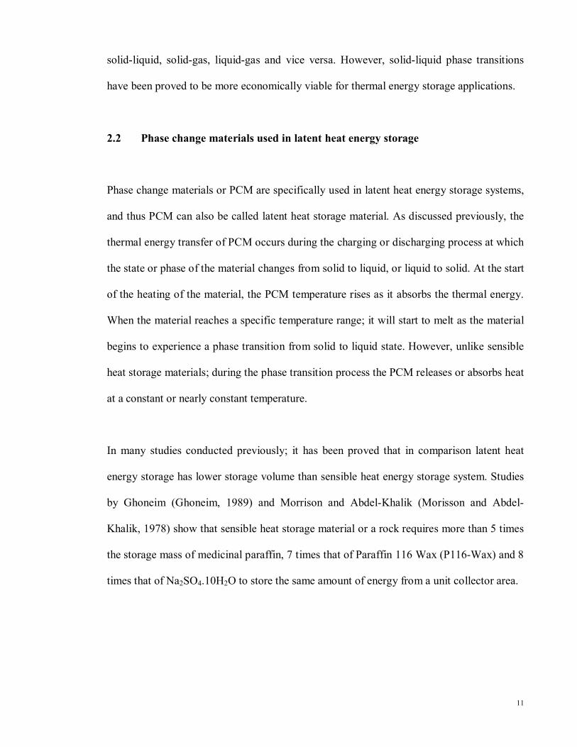
solid-liquid, solid-gas, liquid-gas and vice versa. However, solid-liquid phase transitions

have been proved to be more economically viable for thermal energy storage applications.

2.2 Phase change materials used in latent heat energy storage

Phase change materials or PCM are specifically used in latent heat energy storage systems,

and thus PCM can also be called latent heat storage material. As discussed previously, the

thermal energy transfer of PCM occurs during the charging or discharging process at which

the state or phase of the material changes from solid to liquid, or liquid to solid. At the start

of the heating of the material, the PCM temperature rises as it absorbs the thermal energy.

When the material reaches a specific temperature range; it will start to melt as the material

begins to experience a phase transition from solid to liquid state. However, unlike sensible

heat storage materials; during the phase transition process the PCM releases or absorbs heat

at a constant or nearly constant temperature.

In many studies conducted previously; it has been proved that in comparison latent heat

energy storage has lower storage volume than sensible heat energy storage system. Studies

by Ghoneim (Ghoneim, 1989) and Morrison and Abdel-Khalik (Morisson and Abdel-

Khalik, 1978) show that sensible heat storage material or a rock requires more than 5 times

the storage mass of medicinal paraffin, 7 times that of Paraffin 116 Wax (P116-Wax) and 8

times that of Na2SO4.10H2O to store the same amount of energy from a unit collector area.

12

2.2.1 Desirable properties of phase change materials

Many authors have experimented with different types of PCMs, subdividing them into

organic, inorganic and eutectic types. There are several properties that governs the selection

of phase change materials which are describe as follows (Abhat, 1983):

Thermal properties

i. Suitable melting temperature range for a particular application.

ii. High latent heat of fusion per unit mass to reduce the amount of material and thus

minimizing the physical size of the thermal energy storage device.

iii. High specific heat in order to provide additional sensible heat storage effects.

iv. High thermal conductivity for assisting in the charging and discharging processes.

Physical properties

i. Stability of phase transition in molecular levels ensures better heat storage.

ii. Small volume changes during phase transition allows for simple container and heat

exchanger geometry.

iii. Low vapor pressure at operating temperatures helps to increase the safety of the

operators during the charging process.

13

Kinetic properties

i. The material used must exhibit little or no supercooling during freezing.

Supercooling affects proper heat extraction from the material.

Chemical properties

i. The material used must posses chemical stability and compatibility with

construction materials of the container.

ii. The material must be non-toxic, non-flammable and non-explosive for safety

concerns.

Economic aspect

i. The material is available in abundance and low-cost.

2.2.2 Classification of PCMs

There are many types of phase change materials for a given temperature range. Fig. 2.2

shows the classification of PCMs that are subdivided into three different classes namely

organic, inorganic and eutectic (Sharma et al., 2009).

These various types of PCMs as illustrated Fig 2.2 have different thermal and physical

properties from one another. The selection of suitable phase change material depends on the

desirable properties as discussed in the previous subsection. However, majority of the phase

14

change material do not possess the recommended properties for an ideal thermal energy

medium and thus thermal enhancers are used to improve any disadvantages that the

medium may have. The following discusses the properties of each subclass of the phase

change material.

Fig. 2.2. Classification of phase change materials.

Inorganic materials

Inorganic materials can be further subdivided into salt hydrate and metallics. These

materials do not show degradation in their latent heats of fusion with cycles of freezing and

melting. Furthermore, they do not supercool noticeably.

Phase Change Material

Organic

Paraffin

Non-Paraffin

Inorganic

Salt hydrate

Metallic

Eutectic

Inorganic-inorganic

Inorganic-organic

Organic-organic

15

i. Salt hydrate

The most commonly used inorganic compounds are the hydrated salts. Suitable

to be used in a wide range of applications, salt hydrates are the most important

group of PCMs and have been studied comprehensively in latent heat thermal

energy storage systems. Salt hydrates are mostly consisting of salt and water,

which mixtures form a crystalline matrix when they solidify. Salt hydrates may

be combined with other components to form eutectic solutions. They have high

latent heats of fusion and high thermal conductivity. Their availability and low

cost made them commercially attractive for heat storage applications. Salt

hydrates have a sharp melting point which increases the efficiency of a heat

storage system and have a lower volume change during melting.

The melting behavior of the salt hydrates can be identified into three types,

which are: (a) congruent, (b) incongruent and (c) semi-congruent melting. The

main problem when using salt hydrates as a medium in thermal energy storage

is the behavior of the melted salt hydrate once it melted incongruently. As the

salt is not entirely soluble in its water of hydration during melting, some of the

salt settles down at the bottom of the container. As a result some fractions of the

salts are not able to recombine with water during the freezing/discharging

process and thus reducing the active volume available for heat storage. This

cycle continues with each melting-freezing process cycle. Fortunately, this

problem can be resolved by encapsulating the phase change material to reduce

separation (Lane and Rossow, 1976), mechanical stirring (Lane, et al., 1978),

using gelled or thickening agents (Telkes, 1975), modifying the chemical

16

composition of the system (Charlsson et al., 1979, Alexiades and Solomon,

1992) or using excess water to prevent supersaturation (Biswas, 1977).

ii. Metallic

Metallic materials; which include low melting metals and metal eutectics are not

widely used due to their heavy weights. Thermal energy storages that employ

metallics however might have an advantage on their physical sizes as metallic

materials have high heat of fusion per unit volume, apart from their higher

thermal conductivities compared to other types of PCMs.

Organic materials

In the past, organic materials such as polyethylene glycol, fatty acid and paraffin were not

favorable due to them being costlier than common salt hydrates and low heat storage

capacity per unit volume. However, the strong advantage of the organic materials over

inorganic materials compensates its disadvantages. Organic materials can melt congruently

in which the constant melting and freezing cycle of the material does not cause any

degradation of its latent heat of fusion and phase segregation in the material. Furthermore,

organic materials can self-nucleate in which the crystallization of the material happens with

little or no supercooling. Organic materials can be further classified into paraffin and non-

paraffin.

17

i. Paraffin

Paraffin wax is a mixture of n-alkanes that has a general formula of CnH2n+2 and

falls within the 20 ≤ n ≤ 40 range (Freund et al., 1982). It is mostly made up of

straight chain n-alkanes CH3-(CH2)-CH3. As the hydrocarbon chain increases,

the melting temperature and heat of fusion of the paraffin wax increase with

longer chain length (Suwondo et al., 1994). Through petroleum distillation,

commercial grade paraffin wax can be obtained and may be used as PCMs in

latent heat thermal energy storage systems. The reliability, predictability, non-

corrosiveness, abundant and easily available at low-cost made paraffin wax an

attractive material to be used in latent thermal energy storage system. They are

chemically inert and stable below 500°C although it can undergo slow oxidation

when exposed to oxygen; thus requiring closed containers (Lane, 1983). Paraffin

wax does not show any degradation in its properties even after 1500 cycles (Liu

and Chung, 2005). For containers that are made up of plastic, some care should

be taken during experiments as paraffin waxes have a tendency to soften some

plastics (Lane, 1983).

Although paraffin waxes show favorable characteristics, they also have a few

unwanted properties. Paraffin waxes have low thermal conductivity in their

solid state and are moderately flammable. These unwanted properties can be

alleviated with modifying the wax and also by using proper container (Sharma

et al., 2009). Furthermore, paraffin waxes are not compatible to some plastic

containers. However, acrylic plastics are chemically resistant of paraffinic

hydrocarbons (Schwartz, 2002).

18

ii. Non-paraffin

Unlike paraffin, non-paraffin organic phase change materials have various

properties with their own each distinction. Buddhi and Sawhney (Buddhi and

Sawhney, 1994) and Abhat et al. (Abhat, et al., 1981) have studied, compiled

and identified various types of fatty acids, esters, glycols and alcohols that are

suitable for thermal energy storage systems. These non-paraffin organic

materials are further subdivided into other non-paraffin organic materials and

fatty acids (Sharma et al., 2009). Although these organic materials have high

heat of fusion, they also have high inflammability which can easily be ignited

when exposed to flames, low flash points, unpredictability at high temperatures

and varying level of toxicity which renders them unsafe if not handled carefully.

Eutectics

A eutectic system is a mixture of two or more chemical compounds or elements, which has

a single chemical composition when mixed in a particular ratio and has a minimum-melting

composition that corresponds to two or more components, each of which melts and freezes

congruently forming a mixture of the component crystals during crystallization (George,

1989). Since eutectic melts and freezes without segregation, the components are not easy to

be separated. The unpredictability of the life expectancy and separation of eutectic

compounds hinders them from being widely used thermal energy storage application.

19

2.3 Geometry of thermal energy storage systems

In this section, a review of various geometrical configurations is presented. These include

rectangular, spherical, cylindrical and finned geometries that have been studied extensively

in the past.

2.3.1 Rectangular geometry

Studies on the use of rectangular geometry for phase change thermal energy storage was

first initiated by Shamsundar and Sparrow (Shamsundar and Sparrow, 1975, Shamsundar

and Sparrow, 1976) by applying fully implicit finite-difference method to the resolution of

the enthalpy equation in square geometry. Studies by (Wang et al., 1999, Hamdan and

Elwerr, 1996, Benard et al., 1985) have shown that the effects of free convection in the

melting layers of PCM in rectangular enclosure are significant. Stritih (Stritih, 2004)

compared the heat-transfer characteristics of a finned rectangular latent heat storage unit

with a plain latent heat storage unit. It was found that during melting and solidification, the

finned unit has an increase in heat transfer rate compared to the plain unit. The author also

noted the effects of natural convection on the increased rate of heat transfer during melting.

The use of fins in rectangular geometry has always been employed to improve the low

thermal conductivities of most PCMs. The PCMs are often used in a thin plate

configuration similar to that of a heat exchanger (Farid and Husian, 1990, Farid et al., 1998,

Halawa et al., 2005).

Works by Lacroix et al. (Lacroix, 1989, Binet and Lacroix, 1998, Lacroix, 2001) showed

that the fusion and natural convection effects in a rectangular cavity can be solved by using

20

a technique similar to the moving mesh method. The simulation studies also show that the

melted fraction from close-contact melting at the bottom of the cavity (dominated by

natural convection) is larger than the melted fraction due to conduction at the top. The

authors noted that the melting process is fundamentally governed by the magnitude of

Stefan number. A study on the effects of convection in close-contact melting of high

Prantdl number substances has also been carried out (Groulx and Lacroix, 2007). Liu and

Groulx (Liu and Groulx, 2011) studied the effects of fins in a rectangular geometry using

octadecane as the phase change material. They found out that the positioning and length of

the fin can increase the heat transfer rate of the PCM in a free convection driven melting

process.

2.3.2 Spherical geometry

The use of spherical geometry in thermal energy storage is often employed in packed beds

where spherical capsules are used as containers for PCMs to increase storage density and

efficiency (Regin et al., 2008). A study on the spherical geometry found that spherical

capsules with small diameters are dominated by conduction heat transfer (Saitoh and Moon,

1998). The authors further noted that for large diameter and high Stefan number cases, the

combined natural convection and close-contact melting effects are significant. Ettouney et

al. (Ettouney et al., 2005) experimented on the heat transfer of paraffin wax in spherical

shells during melting and solidification. They found that the Nusselt number for melting is

greatly influenced by the sphere diameter, low dependency on the air temperature and the

air velocity effects however can be neglected. Furthermore, the authors noted that spheres

with larger volumes allow for free motion inside the shells where the cooler and hotter

21

molten wax is freely moving. This is attributed to the increase of natural convection cells in

the PCM.

A study to enhance the heat transfer performance of PCMs in spherical geometry has also

been carried out by Ettouney et al. (Ettouney et al., 2006). Together with paraffin wax;

metal beads were filled into the spherical capsule. A single capsule is then placed in a

stream of hot/cold air. A comparison study between capsules with pure paraffin wax and

paraffin mixed with metal beads was performed. It was found that the enhancement

technique by using metal beads shows a reduction of melting and solidification times by up

to 15%.

2.3.3 Cylindrical geometry

Cylindrical geometry in various practical applications such as food processing, casting

processes and thermal storage systems is deemed to be significantly convenient (Jones et

al., 2006). Since the beginning of computer age and the rapid increase of computing power,

numerical simulations based on fixed or moving grid methods have been used to solve

solid-liquid phase change problems (Brent et al., 1988, Simpson and Garimella, 1998,

Beckett et al., 2001). Experimental data on a coolant-carrying tube analysis (Sparrow and

Hsu, 1981) has also been compared to a numerical validation done by Zhang and Faghri

(Zhang and Faghri, 1996) in which the results were found to be in good agreement. Jones et

al. (Jones et al., 2006) employed photographic and digital image processing techniques

along with enthalpy method to study the melting of a moderate-Prandtl-number material in

a cylindrical enclosure which aims to set up a benchmark experimental measurements in

order to validate numerical codes. Validation of a numerical model based on particle-

22

diffusive model and the enthalpy method in the melting of particle-laden slurry in a

cylinder was performed (Suna et al., 2009). Analysis between the numerical study and

experiment shows a reasonable agreement. The authors also noted that the flow and heat

transfer characteristics of the melt are influenced by the solid particles and the migration of

particles during melting cannot be sufficiently described by the particle-diffusive model

alone.

Prakash et al. studied a solar water heater storage unit which contains a layer of phase

change material at the bottom (Prakash et al., 1985). Due to the low thermal conductivities

of most PCMs, Farid (Farid, 1986) proposed a method of using many layers of PCMs with

different melting temperatures in order to improve the performance of thermal energy

storage devices for solar heating applications. Works by Farid and Kanzawa (Farid and

Kanzawa, 1989) and Farid et al. (Farid et al., 1990) applied the proposed method by

developing a heat storage module which consists of vertical tubes filled with materials

having different melting temperatures. Jian-you (Jian-you, 2008) performed an

experimental and numerical investigation of a thermal energy storage device that has a

triplex concentric tube with PCM filled in the middle channel and hot/cold heat transfer

fluids are filled in the other two channels. Furthermore, a temperature and thermal

resistance iteration method was developed by the author to analyze the melting and

solidification of PCM in the triplex concentric tube in which when compared to

experimental data shows a good agreement.

23

2.3.4 Finned geometry

There have been numerous studies conducted in order to improve the performance of phase

change materials due to most of the available PCMs have unsatisfactorily low thermal

conductivity. This leads to the slow melting and solidification process in thermal energy

storage devices, and in turn reducing the efficiency of the system. Due to the low cost of

construction, simplicity and ease in fabrication; most of heat enhancement techniques

studied in the literatures are based on the configurations of fins embedded in the PCM side.

Lamberg and Siren (Lamberg and Siren, 2003) studied a simplified analytical model for

melting in a semi-infinite PCM storage with an internal fin to predict the solid-liquid

interface location and temperature distribution of the fin. The results show a good

agreement between analytical and numerical results. Reddy (Reddy, 2007) analyzed a

double rectangular enclosure for solar water heating system with PCM. The system

performance with 4, 9 and 19 fins inside the PCM was investigated. The author observed

that the system with 9 fins shows an optimal performance with 95% of the PCM has melted

during the study. For other literatures, Table 2.1 summarizes some studies on finned

geometry thermal energy storage devices.

24

Table 2.1: Studies on finned geometry of thermal energy storage devices.

Reference System geometry

Geometry/configurat-ion of fins

Process Remarks

(Lamberg and Siren, 2003)

Rectangular Rectangular/placed between two vertical heated surfaces

Melting An analytical model was presented to predict the position of the mushy region during melting of PCM.

(Lacroix and Benmadda, 1998)

Rectangular Rectangular/ vertically emerged from bottom of heated surface

Melting Melting is enhanced with increasing Rayleigh number. For a given Rayleigh number, melting time is minimized with an optimal distance between the fins.

(Reddy, 2007)

Rectangular Rectangular/emerge from the top of an inclined heated surface

Melting An optimum performance with 9 fins configuration was observed with 95% of PCM was melted.

(Seeniraj et al., 2002)

Shell and tube

Annular/circling the HTF tube

Melting Numerical study using enthalpy based method shows a considerable increase in the energy storage with the addition of fins.

(Zhang and Faghri, 1996)

Shell and tube

Rectangular/internal, longitudinal

Melting Melting volume fraction can be increased significantly with the increase of thickness, height and number of fins.

(Liu et al., 2005)

Shell and tube

Spiral twisted tape/spans and circling the HTF tube

Solidifi-cation

The new fin improves conduction and natural convection of the PCM by up to 250% during solidification. A fine fin results in more effective enhancement.

25

2.4 Heat transfer in phase change materials

This section describes the heat transfer characteristics of heat transfer process in phase

change materials used in latent heat thermal energy storage systems.

2.4.1 Stefan problem

Stefan (Stefan, 1891) studied the melting of ice as to investigate the phenomenon of heat

conduction or diffusion involving a phase change or a moving boundary problem. This type

of problem has been collectively referred to Stefan problem. Solving the Stefan problem

involves determining the location of solid-liquid interface boundary that changes with time.

Consider a one-dimensional heat conducting material which occupies a semi-infinite half

space 0 < � < ∞ that can exist either in solid or liquid state. Initially, the material is in

solid state and at its melting temperature ��. At time � = 0 thermal energy in the form of

constant wall boundary temperature ��(> ��) is supplied at � = 0. Therefore, the material

melts and the solid-liquid interface �(�) moves away from � = 0 as the melting process

occurs. The temperature distribution of �(�, �) in the molten region 0 < � < �(�) is

governed by the heat conduction equation given by (Esen and Kutluay, 2004):

��

��= �

��

��, 0 < � < �(�), � > 0

With boundary conditions given as:

��

��= −ℎ��, � = 0, � > 0

(2.6)

(2.7)

26

�(�(�), �) = ��, � = �(�), � > 0

where � and � is the liquid thermal conductivity and density respectively (assumed

constant), � is the specific heat capacity and ℎ� is the prescribed function of � > 0. The right

hand side term of Eq. (2.6) describes the heat flux in the decreasing temperature direction

and thus it has a positive magnitude due to the heat flow which moves in the positive X

direction, 0 < � < ∞.

The heat balance equation governs the location of the moving solid-liquid interface. It is

also known as the Stefan condition and can be described as (Esen and Kutluay, 2004, Dutil

et al., 2011):

�� (�)

�� = ��

�� − ��

��, � = �(�), � > 0

where L is the latent heat of fusion of the material, �(�) is the location of solid-liquid

interface as a function of time, the subscripts s and l denote the solid and liquid phases of

the material. At � = 0, the material is in the solid state only. Therefore no liquid region

exists in the material, �(0) = 0.

2.4.2 Solving the Stefan problem

The behavior of the phase change materials during melting or solidification proves to be

difficult to solve due to the non-linear nature of the moving solid-liquid interface and

different thermophysical properties of the two phases. Classical approach on the Stefan

(2.8)

(2.9)

27

problem only involves pure conduction in semi-infinite medium (Carslaw and Jager, 1973,

Lauardini, 1981) before natural convection effects are considered in later years.

Analytically, techniques such as isothermal migration (Keung, 1980), heat balance integral

(Goodman, 1958, Yeh and Chung, 1975), source and sink method (Buddhi, et al., 1988)

have been used to solve Stefan problem. However, these techniques are limited to one-

dimensional problem as they are proven to be very complicated when applied to multi-

dimensional analyses. Through numerical methods, either by using finite element or finite

difference has been shown to be more powerful in solving the Stefan problem. In general,

there are two numerical approaches of solving the moving boundary problems: (a) Adaptive

mesh or (b) fixed grid technique.

Adaptive mesh technique

The element sizes used in numerical analysis may be refined to increase the model grid

density in order to improve the accuracy of the calculation. This technique may be used to

increase the grid density in areas of the numerical domain where the melting or

solidification process is taking place. However, the highly refined mesh elements may not

be needed in other areas of the domain. A local mesh refinement method, called the h-

method is used to add or remove grid points subjected to the required accuracy on a

uniform grid for every iteration (Provatas et al., 1999, Ainsworth and Oden, 2000). Another

method, called the r-method (relocation method); also known as the moving mesh method

starts with a uniform mesh in the domain. The mesh points are then moved, keeping the

mesh topology and number of mesh points fixed as the solution evolves. The deformation

of grid is done by tracking the rapid evolution of the solution or one of its higher order

derivatives (Mackenzie and Mekwi, 2007, Tan et al., 2007).

28

Fixed grid technique

Through the use of an enthalpy method, the phase change problem is simplified since the

governing equation is similar for the two solid/liquid phases, the solid-liquid interface

condition is automatically achieved and the method creates a mushy zone between the two

phases. The mushy zone allows for smooth continuity between the solid-liquid phases

during the numerical analysis. The enthalpy formulation has been used extensively and is

one of the most popular fixed grid methods for solving the phase change problem. The

enthalpy function h as a function of temperature is given by (Voller, 1990):

��

��= ∇[��(∇�)]

where H is the total volumetric enthalpy and �� is the thermal conductivity of phase k in

PCM. Eq. (2.10) describes the energy conservation of a phase change process in terms of

the total volumetric enthalpy and temperature for constant thermophysical properties. H is

the sum of sensible and latent heats, and can be given as:

� (�) = ℎ(�) + ��(�)�

The enthalpy ℎ is defined as:

ℎ = � ��

��

(2.10)

(2.11)

(2.12)

29

For isothermal phase change process, the liquid fraction � is given by:

� = �

0, � < ��0 − 1, � = ��1, � > ��

An alternative form of Eq. (2.10) can be produced by using Eqs. (2.11) and (2.12). For a

two-dimensional heat transfer in the PCM is given by:

��

��=�

��ℎ

�� +

�

��ℎ

�� − ��

��

��

where � is the thermal diffusivity of the material and � is the density of the material.

A study to compare simulation methods for a phase change model in a rectangular cavity

was performed by Lacroix and Voller (Lacroix and Voller, 1990). They conclude that the

use of moving mesh method is limited due to the need of coordinate generator at each time

increment. The fixed grid technique on the other hand must be finer for a unique melting

temperature material. Bertrand et al. (Bertrand et al., 1999) have also carried out a

comparison study between moving and fixed grid methods. They found out that the

adaptive mesh method performs better than the fixed grid technique. However, a scenario

where the solidification occurs at macroscopic surface level is better suited for the enthalpy

method.

(solid) (mushy) (liquid)

(2.13)

(2.14)

30

CHAPTER 3

METHODOLOGY: GEOMETRICAL DESIGN AND GOVERNING

MATHEMATICAL EQUATIONS

This chapter includes the discussions on the geometrical arrangement, dimensions and the

materials used for the numerical studies on the LHTES. Also in this chapter, the governing

physical equations and mathematical formulations used by COMSOL Multiphysics

software for the thermophysical processes that are used in the numerical studies are

presented in the following subsections.

3.1 Latent heat thermal energy storage device geometrical arrangement,

dimensions and materials

The drawing of the cylindrical LHTES device used for the numerical studies is shown in

Fig. 3.1. The full geometrical dimensions of the LHTES are tabulated in Table 3.1; together

with the list of materials used for each component. Also, the materials’ properties are

presented in Table 3.2.

Table 3.1: Latent heat thermal energy storage device dimensions and materials.

Component Material Outer radius,

mm Inner

radius, mm Thickness,

mm Length,

mm Tube Copper 40 30 10 1000 Fin Copper 240 40 5 - Container Acrylic

plastic 290 280 10 1000

31

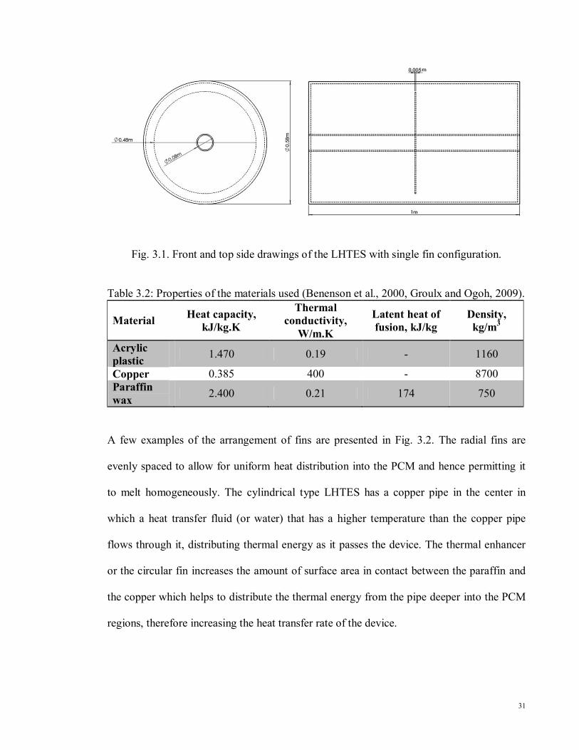
Fig. 3.1. Front and top side drawings of the LHTES with single fin configuration.

Table 3.2: Properties of the materials used (Benenson et al., 2000, Groulx and Ogoh, 2009).

Material Heat capacity,

kJ/kg.K

Thermal conductivity,

W/m.K

Latent heat of fusion, kJ/kg

Density, kg/m3

Acrylic plastic

1.470 0.19 - 1160

Copper 0.385 400 - 8700 Paraffin wax

2.400 0.21 174 750

A few examples of the arrangement of fins are presented in Fig. 3.2. The radial fins are

evenly spaced to allow for uniform heat distribution into the PCM and hence permitting it

to melt homogeneously. The cylindrical type LHTES has a copper pipe in the center in

which a heat transfer fluid (or water) that has a higher temperature than the copper pipe

flows through it, distributing thermal energy as it passes the device. The thermal enhancer

or the circular fin increases the amount of surface area in contact between the paraffin and

the copper which helps to distribute the thermal energy from the pipe deeper into the PCM

regions, therefore increasing the heat transfer rate of the device.

32

Fig. 3.2. Geometrical representations of 0, 1, 3 and 7 fins configuration of LHTES.

3.1.1 Selection of fins

To support the weight of the PCM in between fins, the circular fin is chosen to have the

thickness of 5 mm and has the outer radius of 240 mm, leaving a 40 mm gap between the

container and the fin. The effects of the thickness of the fin and the gap may result in a

different outcome for different thicknesses and gap lengths. However, these two variables

are not in the scope of study for this research.

33

3.2 Heat transfer, fluid flow and phase change processes

The following subsections cover the fundamental thermophysical laws that govern the

system. The boundary and initial conditions are also presented in order for each of the

processes to be solved.

3.2.1 Heat transfer process

Convection heat transfer by thermal fluid

When the thermal fluid or water flows through the tube pipe, convection mechanism

transfers the heat from within the fluid to the wall of the copper pipe. Temperature

distribution in any system can be obtained by solving the energy equation that governs the

system. In the case of a pipe, the energy equation in cylindrical coordinates for constant

properties is given by (Deborah and Michael, 2005, Jiji, 2009b):

��

��+ ��

��

��+��

��

��+ ��

��

�� = � �

1

�

�

��

�� +

1

��

��+��

�� + ��

Where � denotes the velocity of the fluid; subscripts r, θ and z represent the radial, angular

and z-direction components of the system, �� and � are the specific heat and thermal

conductivity of the fluid. The heat generated by viscous dissipation �� is trivial for the

current study. The flow field of the thermal fluid can be solved using the Navier-Stokes and

continuity equations which are heavily discussed by (Jiji, 2009b). Together with Eq. (3.1),

(3.1)

34

the convection heat transfer problem can be solved by the following boundary and initial

conditions:

�(�, �, � = 0) = ��

�(�, � = 0, �) = ��

��

��

= 0

Conduction heat transfer

In the current study, the heat transfer in the PCM is assumed to only be in the conduction

mode; in which the free convection effects due to the liquid PCM is neglected to reduce

computing time. Furthermore, at higher number of fins configuration the volume of PCM

between the fins is small, reducing the effects of the natural convection. Nevertheless, the

general axisymmetric energy equation in cylindrical coordinate for constant properties can

be given by (Deborah and Michael, 2005, Jiji, 2009b):

��

��= � �

1

�

�

��

�� +

��

��

Eq. (3.5) can be solved by using the initial condition given by Eq. (3.2) at � = 0. The

exterior of the container is insulated and therefore the boundary condition for the surface of

(3.2)

(3.4) (axial symmetry)

(3.5)

(3.3)

35

the system is governed by �� ⃗⁄ = 0, where ��⃗ describes the fluid flow normal to the

outside surface.

3.2.2 Fluid flow process

As discussed earlier, the flow field of the thermal fluid is governed by the Navier-Stokes

and continuity equations. For an incompressible axisymmetric flow, the continuity equation

in cylindrical coordinates is given by (Deborah and Michael, 2005, Jiji, 2009b, Flandro et

al., 2011):

1

�

�

��(��) +

�

��(��) = 0

The incompressible axisymmetric Navier-Stokes equations in the radial and z-direction

components are given by (Deborah and Michael, 2005, Jiji, 2009b, Flandro et al., 2011):

�:� ��+ ��

��

+ �� = −

��

��+ � �

1

�

�

�� +

��

−�� + ��

�:� ��+ ��

��

+ �� = −

��

��+ � �

1

�

�

�� +

��

� + ��

where P denotes the pressure and g is the gravity acceleration. The initial and boundary

conditions are given as:

��(�, � = 0) = ��

(3.6)

(3.7)

(3.8)

(3.9)

36

��(� = 0, �) = ��

�� = 0

��

= 0

Where �� is the initial inlet velocity of the thermal fluid. Since there is no velocity relative

to the boundary, the thermal fluid in the copper pipe has a no-slip condition at the wall.

3.2.3 Phase change heat transfer process

During the phase change heat transfer process, or melting of the phase change material; the

conduction occurs in the phase change can be described as a moving boundary or free

boundary problems. The transfer of energy during this process must be accounted for to

analyze the amount of energy that can be stored during the simulation. The general

interface energy equation is given by (Jiji, 2009a, Naterer, 2003):

��

− ��

= ��

��

Where X denotes the position of the melting front and L denotes the latent heat of fusion.

Therefore, Eq. (3.13) describes the balance between the difference of solid and liquid

phases’ heat fluxes with the latent heat absorbed by the PCM during the melting process.

(3.11)

(axial symmetry) (3.12)

(3.13)

(3.10)

(no-slip at the wall)

37

3.3 Numerical analysis

The application of computer simulation through the use of finite element method (FEM)

has become a vital part of engineering and science. Developing new products and

optimizing designs by digitally analyzing the components have accelerated innovations and

breakthroughs over the recent years. This part of the chapter explains the use of COMSOL

Multiphysics to numerically simulate the thermal behavior of the latent heat thermal energy

storage system having transient partial differential equations, either linear or non-linear

thermophysical systems that govern the various processes in the LHTES.

3.3.1 Numerical model

The geometry of the numerical model is first created in the COMSOL Multiphysics space

environment by applying the 2D axisymmetrics model configuration. The physics of the

study are then determined. For the current study, the conjugate heat transfer physics

interface in the heat transfer module is selected during the set-up of the model; which

combines the heat transfer analysis of solid and fluid systems. The module also includes

turbulent flow model including fast moving fluids that have a high Reynolds number.

Afterwards, the initial and boundary conditions of the physics applied to the geometry are

determined. The geometry computational domains are discretized into triangular mesh

elements and time-steps are carefully selected. Lastly, the numerical study is executed by

running the simulation.

38

All of the heat transfer and fluid flow governing equations are solved by COMSOL

Multiphysics software during the simulation by applying the initial and boundary

conditions that are defined earlier. The following subsections describe the numerical model

and the conditions that are applied for the numerical simulation.

Initial conditions for the system

The initial values node in the model builder of the COMSOL software is used to define the

initial conditions for the velocity field, pressure and temperature as well as for the

turbulence variables and radiosity, if applicable (COMSOL, 2011). The following are the

applied initial conditions for the study:

�� = ��

� = ��

Where �� denotes the velocity field in the z-direction and �� denotes the initial thermal

fluid velocity.

Heat transfer module

Heat transfer in solids node: The node adds the heat equation for conductive heat transfer in

solids. It essentially uses the same heat conduction equation of Eq. (2.6).

(3.14)

(3.15)

39

Temperature node: The temperature node defines the thermal fluid inlet temperature

boundary condition which is given as (COMSOL, 2011):

� = ��

Heat continuity node: The continuity node prescribes that the temperature field is

continuous across different domains where the boundaries are matched. This heat

continuity boundary condition permits the heat flux to travel from one internal boundary to

another, simulating the continuous heat flow from the source and finally to the phase

change material. The governing mathematical equation is given as (COMSOL, 2011):

��⃗.(�� − ��) = 0

Where �� and �� denote the calculated heat fluxes of two adjacent mesh elements. The heat

flux � is defined as (COMSOL, 2011):

� = −�∇��⃗�

Thermal insulation node: The node is the default boundary condition for all heat transfer

interfaces. Naturally, the insulation boundary equation describes the temperature gradient

across the boundary to be zero at which the temperatures for adjacent boundaries are equal.

The thermal insulation boundary equation is given as (COMSOL, 2011):

��⃗.��∇��⃗�� = 0

(3.16)

(3.17)

(3.18)

(3.19)

40

Fluid flow module

Inlet node: The node defines the boundary condition of a fluid flow at an inlet. The normal

inflow velocity is selected and its governing equation is given as (COMSOL, 2011):

��⃗ = −��⃗

Wall node: The node denotes the wall boundaries in a fluid-flow simulation. As explained

earlier, the thermal fluid velocity in the radial component is zero; hence a no-slip condition

exists at the pipe wall. The boundary condition is given as (COMSOL, 2011):

��⃗� = 0�⃗

The Wall node represents wall boundaries in a fluid-flow simulation. It includes several

options to describe different type of walls. The default condition is that for a smooth wall.

Outlet node: The node denotes boundaries with outwards flow in a fluid-flow simulation.

The node can be used to define the boundary condition of the thermal fluid in terms of its

pressure, velocity or stress condition. For the current study, “pressure, no viscous stress” is

applied for the outlet boundary condition. This condition specifies vanishing viscous stress

along with a Dirichlet condition on the pressure which gives total control of the pressure

level at the entire boundary. The mathematical governing equations are given as

(COMSOL, 2011):

(3.20)

(3.21)

41

� = �� = 0

��∇��⃗� + (∇��⃗�)��⃗ = 0

Modeling the phase change process

Energy is needed in large quantity during the phase change process to melt the PCM.

Furthermore, the position of the melting interface during the solid-liquid phase change

process must be recognized and solved. These two factors can be solved numerically using

the effective heat capacity method. The effective heat capacity, ��,�� of the paraffin wax

can be defined by (Lamberg et al., 2004):

��,�� =�

(�� − ��)+��,� + ��,�

2

Where � denotes the latent heat of fusion, �� is the temperature at the start of the phase

change and �� is the temperature when the phase change process ends. Knowing that the

solid and liquid heat capacities for paraffin have the same values, the modified heat

capacity can be written as (Lamberg et al., 2004):

��,��

2.4kJ/(kg.K)� < ��

60.5kJ/(kg.K)�� < � < ��2.4kJ/(kg.K)� > ��

(3.22)

(3.23)

(3.24)

(3.25)

42

A continuous step function is created in the COMSOL software to incorporate Eq. (3.25) in

order to solve the phase transition problem numerically. By adopting the method introduced

by Groulx and Ogoh (Groulx and Ogoh, 2009); the following function is used in the

material node of the COMSOL software (COMSOL, 2011):

��,�� = �� + ��,�� ∗ (��2ℎ�(� − ��, ��) − ��2ℎ�(� − ��, ��))

Where ��2ℎ� is a smoothed step transition function in COMSOL Multiphysics.

Fig. 3.3. The modified heat capacity of the paraffin wax defined from temperature range of

290 K to 350 K.

0

10

20

30

40

50

60

70

290 300 310 320 330 340 350

Hea

t ca

pac

ity

(kJ/

kg.

K)

Temperature (K)

(3.26)

43

The graph shown in Fig. 3.3 illustrates the modified heat capacity of the paraffin wax after

applying Eq. (3.25) into Eq. (3.26) which can then be written as (Groulx and Ogoh, 2009,

COMSOL, 2011):

��,�� = 2.4 + 60.5 ∗ (��2ℎ�(� − 313, 0.02) − ��2ℎ�(� − 316, 0.02))

The plot shown in Fig. 3.3 illustrates the non-linear characteristic of the modified heat

capacity that changes its value during the melting of the PCM. This method forces the

COMSOL software to change the heat capacity value of the PCM from a constant value of

2.4 kJ/kg.K in the solid (T < 313K) and liquid state (T > 316K) to 60.5 kJ/kg.K in the

melting phase (313K < T < 316K).

(3.27)

44

CHAPTER 4

VALIDATION OF PHASE CHANGE PROCESS

This chapter describes about an analytical validation of numerical results data obtained

from the simulation of heating a semi-infinite paraffin slab. The numerical study is done to

simulate the phase change process of paraffin taking place inside the thermal energy

storage. It is important to validate the data analytically in order to support the results

obtained through the numerical studies on the latent heat thermal energy storage system in

the next chapter. For greater accuracy, a mesh convergence study is performed to assure

better numerical results obtained from the simulations.

4.1 Analytical Study

Phase change heat transfer that occurs in any PCM thermal energy storage is a well-known

problem that can be encountered naturally in many thermophysical processes such as

melting of ice, freezing of foods, solidification of metals and other various natural

reactions. It is a transient, non-linear phenomenon in which a moving solid-liquid interface

exists in the material during the phase change process. This moving boundary problem, or

also known as Stefan problem, requires solving the fusion or heat conduction in an

unknown region during the melting or solidification process. Furthermore, the nonlinearity

of the process poses some difficulty in mathematical formulations and therefore simpler

analytical solution in a simple system and geometry having simple boundary conditions is

always favorable in any analysis. For a one-dimensional free and moving boundary

45

problem, Neumann presented an analytical solution to the classical Stefan’s problem in a

very simple formulation (Gupta, 2003).

Fig. 4.1 shows the schematic diagram of a simplified one-dimensional analytical model that

was analyzed. The model is used in the analytical validation of the numerical results data

obtained for a one-dimensional transient solid-liquid phase change process. The semi-

infinite model of a paraffin wax slab is initially assumed to be at its melting temperature

point, Tm. As such, an increase in its temperature will change its current solid state to liquid

state.

Fig. 4.1. One-dimensional analytical moving boundary phase change problem.

The following assumptions were made for the analysis, in which Stefan’s problem is

defined. The assumptions are made similar for the numerical analysis:

1. The wall temperature, Tw and the phase change material temperature in its solid

state are assumed to be at the melting temperature of the PCM, thus Tw = Tm.

2. The only heat transfer mechanism during the melting of the PCM is conduction.

3. The entire walls of the PCM are insulated, except for the heated wall.

46

4. Distribution of temperature is one-dimensional and in the x-direction.

5. The thermophysical properties of the PCM material are independent of temperature,

in which for the current study the heat capacities for solid and liquid phases are

equal.

The boundary conditions are given as follow (Gupta, 2003):

1. Wall temperature: �(� = 0, � > 0) = �� (4.1)

2. Melting front temperature: �(� = �(�), � > 0) = �� (4.2)

where �(�) is the solid-liquid melting interface position.

During melting, the transient energy equation in the liquid phase is governed by (Gupta,

2003, Massoud, 2002, Jiji, 2009a):

��=1

��

��

where �� is the liquid thermal diffusivity, which can be defined as (��,�)/��.

The moving solid-liquid interface in the system is influenced by the heat flux of the liquid

phase at the melting interface and the magnitude of latent heat of the phase change material.

The following equation defines the melting front energy balance (Gupta, 2003, Massoud,

2002, Jiji, 2009a):

−��(�)

��= ��

��(�, �)

��

where � is the latent heat of fusion of the material.

(4.3)

(4.4)

47

By solving Eqs. (4.1) to (4.4), the transient temperature distribution in the liquid phase can

be obtained from the following equation (Gupta, 2003, Massoud, 2002) :

��(�, �) − �� − ��

=

��

2��

��(�)=��(�)

��(�)

The similarity variable � is defined as:

� =�

2��

Whereas, the constant � can be obtained by referring to Eq. (4.4) (Gupta, 2003, Massoud,

2002):

��erf(�) =

��

√�=��,�(�� − ��)

�√�

Referring to Eq. (4.7), the Stefan number, �� is defined as the following equation:

�� =��,�(�� − ��)

�

For further validation purposes, the position of the melting front as a function of time,

measured from the wall at � = 0, can be calculated by using the following equation

(Massoud, 2002):

�(�) = 2��

(4.5)

(4.6)

(4.7)

(4.8)

(4.9)

48

The rate of energy stored through the phase change process due to the heat transferred at

the melting interface can be given as (Massoud, 2002):

�[�(�)]= ��

= −��

√�= −��(�)

where ��(�) is the melting front velocity obtained from Eq. (4.9).

4.2 Numerical Study

The numerical simulation in this section attempts to solve Stefan problem through the use

of pure conduction modeling method. The transient study simulates a 21 hour long heating

of a paraffin wax slab. Fig. 4.2 shows the meshed diagram of a 2D semi-infinite slab of the

PCM which has the dimension of 0.3 m in width and 0.1 m in height. Similar to the

previous section, the PCM was initially set to the melting temperature of 313 K to instantly

melt the material when there is an increase of temperature. The thermal boundary

conditions of the slab are defined in such a way that only the left wall is heated with

temperature of 350 K while the other wall surfaces are insulated. As previously defined, the

latent heat of fusion at the melting interface is solved by using the modified heat capacity as

shown in Eq. (3.27).

Before the numerical results data from the simulation can be analyzed, a mesh convergence

study was carried out to increase the accuracy of the results and independent of the mesh

element sizes. Six different element sizes were tested and their sizes, numbers, degrees of

freedom and simulation times are illustrated in Table 4.1. During the transient study, the

(4.10)

49

time step is carefully chosen to ensure that the simulated temperature increase does not

overshoot the phase change region, where the melting process is taking place. As shown in

Eq. (3.27), the modified heat capacity forces the COMSOL software to solve the system

non-linear. Thus, by adopting the COMSOL time-step technique introduced by (Groulx and

Ogoh, 2009), the time step for the transient study must be less than 350 seconds, for a total

simulated time of 75000 seconds or 21 hours.

Fig. 4.2. Schematic diagram of the 2D slab of paraffin wax.

Table 4.1: Various mesh element sizes used for the simulation.

Element size (mm)

No. of elements Number of DOFs Simulation time (s)

20 188 417 12 s 10 790 1661 17 s

5 3036 6233 26 s 3 8470 17209 43 s

0.6 229910 461155 274 s 0.5 313020 627641 384s

50

Fig. 4.3. Simulated 2D surface temperature plot. Simulated time: 21 hours.

The numerical solution after 21 hours of simulated time is presented in the Fig. 4.3. The

horizontal line P-P, 0.12 m in length; is the linear region at which the analytical

temperature profile will be compared to the numerical temperature profile. The geometrical

dimension of the slab is justified as only about a quarter of the whole system experiences

temperature changes, therefore simulating a semi-infinite system.

Fig. 4.4 shows the temperature distribution profile along the linear region of line P-P after a

simulated time of 3 hours using various mesh element sizes. The convergence study shows

that the results converge at element size of 0.6 mm; with reduction of element size to 0.5

51

mm displays no noticeable changes and therefore element size of 0.6 mm is chosen for

simulation.

Fig. 4.4. Temperature distribution profile along section P-P for various mesh element sizes.

Simulated time: 3 hours.

The temperature history of points A, B, C and D (with distances from the heated wall 0.035

m, 0.025 m, 0.015 m and 0.005 m respectively) after a simulated time of 18 hours is shown

in Fig. 4.5. The figure shows that the four different points demonstrate proper phase change

processes. As previously defined, the paraffin wax melts over a 3 K temperature range. At

point A, melting process starts at the temperature of 313 K and increases until 316 K for

duration of 3 hours at which after the period an inflexion point is observed. This is expected

for a phase change material undergoing a phase change process. However, the inflexions on

the other temperature graphs of point B, C and especially D are less noticeable as the

310

315

320

325

330

335

340

345

350

0 0.02 0.04 0.06 0.08 0.1 0.12

Tem

per

atu

re (

K)

Distance from the heated wall (m)

10 mm

20 mm

5 mm

3 mm

0.6 mm

0.5 mm

Mesh element sizes

52

distance between the heated wall and the points are reduced; the rate of temperature

increase is higher.

Fig. 4.5. Temperature history of points A, B C and D. Simulated time: 18 hours.

Fig. 4.6 shows the temperature distribution along section P-P after simulated times of 0.8,

3, 6, 9, 12, 15 and 18 hours. The numerical results show that 0.017, 0.034, 0.049, 0.060,

0.068, 0.076 and 0.082 m of the phase change material were fully melted (� > 316K)

during these 7 time periods respectively. This validates an accurate simulation of heat

conduction along the length of the melted PCM.

310

315

320

325

330

335

340

345

350

0 3 6 9 12 15 18

Tem

per

atu

re (

K)

Time (Hr)

Point A Point B Point C Point D

53

Fig. 4.6. Temperature distribution profile for various simulated time.

4.3 Validation

Fig. 4.7. Comparison of numerical and analytical temperature distribution profiles for

various simulated times.

310

315

320

325

330

335

340

345

350

355

0 0.02 0.04 0.06 0.08 0.1

Tem

per

atu

re (

K)


0.8 hr

3 hr

6 hr

9 hr

12 hr

15 hr

18 hr

310

315

320

325

330

335

340

345

350

355

0 0.02 0.04 0.06 0.08 0.1

Tem

per

atu

re (

K)


Num. 0.8 hr

Num. 3 hr

Num. 6 hr

Num. 9 hr

Num. 12 hr

Num. 15 hr

Num. 18 hr

Ana. 0.8 hr

Ana. 3 hr

Ana. 6 hr

Ana. 9 hr

Ana. 12 hr

Ana. 15 hr

Ana. 18 hr

54

Fig. 4.7 shows the comparison between the analytical and numerical temperature profiles

for various simulated time. By using Eqs. (4.5) to (4.7), the analytical results obtained from

the calculation of these equations show a good agreement with the numerical results

obtained from the simulations. However, the analytical results for longer periods of time (6,

9, 12, 15 and 18 hours) tend to under predict the numerical results data. This is due to the

under prediction of the total heat flux which reduces the melting rate for the analytical

calculation, and thus resulting in lower temperature compared to the numerical simulation.

This can be simply explained through the different mathematical approach of both of these

models in which the analytical analysis uses a single constant temperature difference during

melting process (Tw-Tm), whereas the simulation melts the PCM over a 3 K temperature

range (313K to 316K).

Fig. 4.8. Melting front position obtained from numerical and analytical studies.


0

0.01

0.02

0.03

0.04

0.05

0.06

0.07

0.08

0 2 4 6 8 10 12

Mel

tin

g f

ron

t p

osit

ion

(m

)

Time (hr)

Numerical

Analytical

55

The plots in Fig. 4.8 demonstrate a comparison of the melting front positions as a function

of time for numerical and analytical studies. The mushy region in the solid-liquid interface

exists between the temperature ranges of 313 K to 316 K, where the melting front position

can be assumed to be in the middle of this mushy region and therefore the temperature of

314.5 K is chosen to represent the position of the melting front. By using Eq. (4.9), the

results of both numerical and analytical data show a good agreement and thus confirming

the simulation of the phase change process.

56

CHAPTER 5

LATENT HEAT THERMAL ENERGY STORAGE: NUMERICAL ANALYSIS

RESULTS AND DISCUSSION

The analytical validation presented in the previous chapter shows that COMSOL

Multiphysics software can sufficiently simulate the phase change process with the use of

the modified heat capacity method. In the following sections of this chapter, the results

obtained from the numerical study of an axisymmetric 2D latent heat thermal energy

storage will be presented and discussed in detail. Before any simulations are carried out, a

mesh convergence study is performed to obtain optimum mesh element size and to achieve

results with the highest possible accuracy from the numerical studies. The numerical

studies are then carried out to investigate the effects of the heat transfer fluid velocities and

the number of the thermal enhancers or fins on the phase change process occurring inside

the LHTES. Furthermore, the maximum possible energy that can be stored in various

configurations of the LHTES is also calculated.

5.1 Numerical analysis – Mesh convergence study

An axisymmetric 2D latent heat thermal energy storage system with similar dimensions and

materials presented in Chapter 3 are illustrated in Fig. 5.1. The mesh convergence study

was set in the beginning to the boundary and initial conditions shown in Table 5.1. These

conditions can be easily set up in the COMSOL software.

57

Table 5.1: Boundary and initial conditions used in the convergence study.

Initial Inlet (water) Outlet Channel

wall Outer

surfaces

Thermal parameters

293.15K 350K Convective flux

Thermal continuity

Insulated

Fluid parameters

0.05 m/s 0.05 m/s

No viscous stress, Po=0

No slip -

Fig. 5.1. A meshed axisymmetric 2D model of the LHTES used in the numerical studies.

The outer surfaces of the model are thermally insulated.

Fluid Flow

58

Similar to the mesh convergence study carried out in the previous chapter, changes to the

mesh element size are performed and refined until converging results can be obtained. The

time-step configuration is also similar to the study done in Chapter 3. The following Table

5.2 shows the various element sizes and the data collected from the 21 hours simulated time

study.

Table 5.2: Various element sizes used in the convergence study and their data.

Element size (mm)

No. of elements Number of DOFs Simulation time (s)

20 4405 3521 357s

16 5248 4281 876s 12 6915 5728 5975s

8 12963 10047 9327s 5 31368 23043 12832s

Fig. 5.2. A 12 fins configuration LHTES with its 2D surface temperature plot used in the

convergence study. Simulated time: 21 hours.

59

Fig. 5.2 shows the temperature plot of a 12 fins configuration LHTES after 21 hours

simulated time. The line P-P shows the region at which the convergence study is carried out

for various mesh element sizes; from 0.02 m down to the smallest size of 0.005 m. The

results of the study are illustrated in the temperature profile plot as shown in Fig. 5.3. As

shown in the figure, the mesh element sizes of 0.02, 0.016 and 0.012 m recorded higher

temperature profile plots compared to the plots of mesh element sizes of 0.005 and 0.008

m. The figure also shows that the temperature is independent of the 0.005 and 0.008

element sizes; which means further reduction in the size of element does not change the

numerical results. Thus, to save time; mesh element size of 0.008 m is chosen for the

subsequent simulation runs.

Fig. 5.3. Temperature profile plots for various mesh element sizes at line P-P.


332

334

336

338

340

342

344

346

348

350

352

0 0.05 0.1 0.15 0.2 0.25

Tem

per

atu

re (

K)

Distance from the tube centerline (m)

0.005 m

0.008 m

0.012 m

0.016 m

0.020 m

Mesh element sizes

60

5.2 Energy stored in LHTES: Integrating COMSOL functions

In order to calculate the possible amount of energy stored in the LHTES device during the

charging (melting) period, volume integration on the phase change material domain is

carried out. The integration calculation is performed on the modified heat capacity ��,��

(which is in the function of the temperature) multiplied with the temperatures in the PCM

region, divided by total volume of the phase change material:

�� = ��∭��,��(�(�, �, �) − ��). ��

∭(�, �, �). ��

Through the finite element analysis simulation, temperature data from every point of the

whole system can be extracted out. Knowing this, the sensible and latent heat contributions

for each temperature range can also be calculated and translating all the information into

COMSOL requires special functions. By restricting the integration on known temperature

ranges for the solid-liquid phase transformation process, the following COMSOL functions

describe the total, sensible and latent energy stored in the LHTES (Groulx and Ogoh,

2009):

�� = �[(�� ∗ (1 − ��2ℎ�((� − 313)[1/�], ��[1/�])) ∗ (� − (293[�])))

(5.1)

+(�� ∗ (��2ℎ�((� − 313)[1/�], ��[1/�]) − ��2ℎ�((�

− 316)[1/�], ��[1/�])) ∗ (20[�]))

+(�� ∗ (��2ℎ�((� − 316)[1/�], ��[1/�])) ∗ (� − (296[�])))] (5.2)

61

�� = �[(��,�� ∗ (��2ℎ�((� − 313)[1/�], ��[1/�]) − ��2ℎ�((�

− 316)[1/�], ��[1/�])) ∗ (� − (313[�])))

�� = �� + ��

The equation of Eq. (5.2) describes the sensible energy stored in the solid (T < 313 K) and

liquid phase (T > 316 K). Whereas, equation of Eq. (5.3) describes the latent energy stored

by the PCM (313 K < T < 316 K).

5.3 Effects of HTF velocities

Simulations on LHTES with fin configurations of 0, 1, 2, 3, 4, 5, 6, 7, 9, 12, 15, 18, 21 and

24 fins were carried out to investigate the effects of various velocities of the HTF on the

thermal behavior of the PCM in the thermal energy storage system. Heat transfer fluid

velocities of 0.01, 0.03, 0.05 and 0.1 m/s (equivalent to mass flow rates of 0.0275, 0.0825,

0.1375 and 0.275 kg/s respectively) were used for the study. The range of mass flow rates

between 0.0825 and 0.1375 kg/s are typically used in solar storage systems. The boundary

and initial conditions used in the numerical studies have been presented in Table 5.1. Also,

only the initial condition of the inlet flow velocity of the HTF is changed accordingly.

The following Figs. 5.4 and 5.5 show the temperature distribution plots for 7 and 15 fins

configuration LHTES with different fluid inlet velocities after 12 hours of simulated time.

Additionally, the Reynolds numbers for each inlet fluid velocity are also presented.

+(��,�� ∗ (��2ℎ�((� − 316)[1/�], ��[1/�])) ∗ (3[�]))] (5.3)

(5.4)

62

Appendix A shows all the temperature distribution plots studied for various number of fins

and the four different HTF velocities.

Fig. 5.4. Temperature distribution plots for the 7 fins configuration LHTES with various

HTF velocities and their Reynolds numbers. Simulated time: 12 hours.

As can be seen from both Figs. 5.4 and 5.5, the heat from the thermal fluid (or water) is

transferred by the conduction heat transfer mechanism through the copper tube and finally

distributed into the phase change material. The heat is largely congregating around the fins

nearer to the inlet, as can be clearly seen in the low thermal fluid velocity of 0.01 m/s. The

heat transferred from the HTF to the fins produces higher temperature regions surrounding

the fins nearer to the inlet. Furthermore, in Figs. 5.4 and 5.5; as the thermal fluid velocity

increases, more heat can be transferred to the PCM, and therefore increases the possible

63

amount of energy that can be stored in the PCM. This can be fundamentally related to the

Reynolds number of the thermal fluid.

Fig. 5.5. Temperature distribution plots for the 15 fins configuration LHTES with various


In Fig. 5.5, the higher number of fins contributed to the larger amount of heat distributed

into the PCM when compared to the temperature distribution plots of Fig. 5.4. The results

show that the possible amount of energy that can be stored increases with higher number of

fins for corresponding velocities. For further clarification, the solid-liquid phase change

interface can be indicated by the contour lines that represent the melting temperature (313

K – 316 K) of the paraffin wax. In Fig. 5.5, much of the PCM region is undergoing the

melting phase, which is comparable to the contours in Fig. 5.4. This suggests higher

amount of energy is being stored. During the charging process, there exists a slow heating

64

zone, or SHZ at which the PCM in this area is slower to receive heat due to the gap

between the fins and the acrylic plastic container, as shown in Fig. 5.6. This area has a

higher thermal resistance than the areas surrounding the fins. Therefore, the PCM in the

SHZ is slower to melt, reducing the melting fraction of the phase change material. The SHZ

area varies from one fin configuration to another, and it highly depends on the number of

fins and the distance between the fins. For the current study, the effects of the distance

between the fins and the enclosure are not in the scope of research, although the SHZ

influences the thermal behavior of the PCM and the overall possible energy storage ability

of the LHTES.

Fig. 5.6. Slow heating zone (SHZ) between the fins and the enclosure reduces the melting

fraction of the PCM.

65

Figs. 5.7 to 5.14 show the total energy stored as a function of time for different LHTES fin

configurations over a 12 hours of simulated charging time for various HTF velocities. The

figures illustrated the variation of total energy stored for 0, 1, 6, 7, 12, 15, 21 and 24 fins

configuration. The results of Fig. 5.7 for the 0 fin configuration show that there is no

significant increase of the total energy stored in the PCM as the HTF velocities increases.

This is due to the high thermal resistance of the PCM. With the addition of fins, the thermal

resistance on the PCM reduces, and the higher thermal energy of the HTF initiates the heat

transfer process into the PCM with the help of the fins. Thus, more energy can be stored in

the PCM and by increasing the HTF velocities; the amount of energy that can be stored is

more evident as clearly shown in the following figures.

Fig. 5.7. Total energy stored for the 0 fin configuration LHTES over 12 hours of simulated

time for various HTF velocities.

0.0

0.5

1.0

1.5

2.0

2.5

3.0

3.5

4.0

4.5

5.0

0 2 4 6 8 10 12

Tot

al e

ner

gy s

tore

d (

MJ)

Time (Hour)

0.01 m/s 0.03 m/s 0.05 m/s 0.1 m/s

66

Fig. 5.8. Total energy stored for the 1 fin configuration LHTES over 12 hours of simulated


Fig. 5.9. Total energy stored for the 6 fins configuration LHTES over 12 hours of simulated


0

1

2

3

4

5

6

7

8

9

0 2 4 6 8 10 12

To

tal

sto

red

en

erg

y (

MJ

)

Time (Hour)

0.01 m/s 0.03 m/s 0.05 m/s 0.1 m/s

0

5

10

15

20

25

30

0 2 4 6 8 10 12

Tot

al e

ner

gy s

tore

d (

MJ)

Time (Hour)

0.01 m/s 0.03 m/s 0.05 m/s 0.1 m/s

67

Fig. 5.10. Total energy stored for the 7 fins configuration LHTES over 12 hours of

simulated time for various HTF velocities.



0

5

10

15

20

25

30

35

0 2 4 6 8 10 12

To

tal

ener

gy

sto

red

(M

J)

Time (Hour)

0.01 m/s 0.03 m/s 0.05 m/s 0.1 m/s

0

5

10

15

20

25

30

35

40

45

0 2 4 6 8 10 12

Tot

al e

ner

gy

stor

ed (

MJ)

Time (Hour)

0.01 m/s 0.03 m/s 0.05 m/s 0.1 m/s

68





0

5

10

15

20

25

30

35

40

45

50

0 2 4 6 8 10 12

To

tal

ener

gy

sto

red

(M

J)

Time (Hour)

0.01 m/s 0.03 m/s 0.05 m/s 0.1 m/s

0

10

20

30

40

50

60

0 2 4 6 8 10 12

Tot

al e

ner

gy s

tore

d (

MJ)

Time (Hour)

0.01 m/s 0.03 m/s 0.05 m/s 0.1 m/s

69



The 2D column chart shown in Fig. 5.15 illustrates the sensible energy stored in the PCM

with different fin configurations and fluid inlet velocities. Table 5.3 tabulates the

percentage of sensible energy increase for various numbers of fins as the HTF velocity

increases (0.01 m/s to 0.1 m/s). The ratio of increase is given by:

��% =��.��/�− ��.��/�

��.��/�x100

Table 5.3: Sensible energy increase in the LHTES for various numbers of fins as the HTF velocity increases.

No. of fins 0 1 2 3 4 5 6 Energy increase (%)

3.5 11.7 12.9 13.0 13.5 17.8 15.7

7 9 12 15 18 21 24 Energy increase (%)

12.4 18.3 35.9 33.5 23.3 26.5 28.4

0

10

20

30

40

50

60

0 2 4 6 8 10 12

To

tal

ener

gy

sto

red

(M

J)

Time (Hour)

0.01 m/s 0.03 m/s 0.05 m/s 0.1 m/s

(5.5)

70

The calculations demonstrate that there exists a steady increase of sensible heat

contribution from 0 to 9 fins configuration with their percentage difference across the

different HTF velocities varies between 3 to 18%. The majority of the PCM is not yet fully

melted for these configurations and the thermal resistance of the phase change material is

hindering the influence of the HTF velocities to distribute heat into the PCM efficiently.

The percentage difference jumps to the highest percentage increase of 36% in the 12 fins

configuration due to the larger fraction of the PCM has been melted, increasing the

penetration of thermal energy into the SHZ areas and thus storing larger sensible heat in the

liquid PCM. As the number of fins increases, the effects of increasing HTF velocities on

the thermal resistance of the PCM are more evident as shown in Fig. 5.15.

Fig. 5.15. Sensible thermal energy stored in various numbers of fins configuration for HTF

velocities of 0.01 m/s, 0.03 m/s, 0.05 m/s and 0.1 m/s. Simulated time: 12 hours.

0

2

4

6

8

10

12

14

16

18

20

0 1 2 3 4 5 6 7 9 12 15 18 21 24

Sen

sib

le e

ner

gy s

tore

d (

MJ)

Number of fins

0.01 m/s 0.03 m/s 0.05 m/s 0.1 m/s

71

The 2D column chart shown in Fig. 5.16 illustrates the latent energy stored in the PCM

with different fin configurations and fluid inlet velocities. Table 5.4 tabulates the

percentage of latent energy increase for various numbers of fins as the HTF velocity

increases.

Table 5.4: Latent energy increase in the LHTES for various numbers of fins as the HTF velocity increases.


6.8 20.5 23.1 23.9 25.9 39.5 32.9

7 9 12 15 18 21 24 Energy increase (%)

24.1 31.1 32.9 21.3 16.6 24.8 25.4

Fig. 5.16. Latent thermal energy stored in various numbers of fins configuration for HTF


0

5

10

15

20

25

30

35

0 1 2 3 4 5 6 7 9 12 15 18 21 24

Lat

ent

ener

gy s

tore

d (

MJ)

Number of fins

0.01 m/s 0.03 m/s 0.05 m/s 0.1 m/s

72

The overall results shown in Fig. 5.16 illustrates that there is a progressive increase of

latent energy percentage difference from the 0 to 12 fin configurations across the increasing

HTF velocities. As the number of fins increases from 15 to 24, the rate of increase of the

latent thermal energy stored in the PCM declines until it appears to be constant for 0.03 m/s

to 0.1 m/s HTF velocities, whereas the 0.01 m/s HTF velocity shows an obvious reduction

in latent heat contribution. This is due to most of the PCM volume has been melted and

changed into the liquid state, reducing the contributions of latent thermal energy.

Furthermore, with the increase of the number of fins, the volume of PCM reduces, hence

reducing the possible amount of latent thermal energy contribution.

The total thermal energy stored in the various fin configurations for various HTF velocities

after simulated charging time of 12 hours are shown in Fig. 5.17. As described in Eq. (5.4),

the total thermal energy stored is the accumulation of the sensible and latent thermal energy

stored in the LHTES. The results shown in Fig. 5.17 illustrates that the total thermal energy

stored in the PCM increases as the number of fins and HTF velocity increases. Table 5.5

shows the percentage difference of the total thermal energy stored for various numbers of

fins as the HTF velocity increases from 0.01 m/s to 0.1 m/s.

Table 5.5: Total energy percentage increase in the LHTES for various numbers of fins as the HTF velocity increases.


5.0 16.2 18.3 18.9 20.5 30.5 26.3

7 9 12 15 18 21 24 Energy increase (%)

19.9 26.9 34.0 25.7 19.0 27.4 26.5

73

Fig. 5.17. Total thermal energy stored in various numbers of fins configuration for HTF


From 0 to 5 fins configuration, the velocity of HTF influences the increase of percentage

difference which starts from 5.0 to 30.5%. However, the percentage difference declines

from the 5 to 7 fins configuration. This is mainly due to the drop in latent heat contribution

which is caused by the melting of the PCM as more areas of the PCM are melted and turned

into the liquid state. This is also apparent in Table 5.4 which shows a reduction of latent

energy difference across the HTF velocities from 5 to 7 fins configuration. Furthermore, a

slow heating zone or SHZ created by the gap between the fins and the container reduces the

contribution of both the sensible and latent heats as the thermal resistance of the SHZ area

is high; creating inconsistencies in the total energy that can be possibly stored. Therefore,

higher number of fins with higher HTF velocity may penetrate the SHZ in order for them to

0

10

20

30

40

50

60

0 1 2 3 4 5 6 7 9 12 15 18 21 24

To

tal

ener

gy

sto

red

(M

J)

Number of fins

0.01 m/s 0.03 m/s 0.05 m/s 0.1 m/s

74

melt, as will be discussed and shown in the next section. Additionally, from 7 to 12 fins

configuration, the percentage difference increases again due to the increase of fin numbers

which reduces the PCM thermal resistance, thus increasing the storage of total thermal

energy. This cycle continues until the 24 fins configuration, where the maximum

percentage difference was recorded for 12 fin configurations with 34% of difference across

the HTF velocity variable.

Fig. 5.18. Melting fraction for various HTF velocities from 0 to 24 fins configuration.


The plots shown in Fig. 5.18 illustrate the melting fractions of the PCM for different HTF

velocities with various numbers of fins. Similar in Chapter 4, the middle temperature of the

solid-liquid phase change interface (T = 314.5 K) is chosen for the calculation of the

melting fraction. The results describe the melting fraction increases as the number of fins

0.0

0.1

0.2

0.3

0.4

0.5

0.6

0.7

0.8

0.9

1.0

0 2 4 6 8 10 12 14 16 18 20 22 24

Mel

tin

g fr

acti

on

Number of fins

0.01 m/s 0.03 m/s 0.05 m/s 0.1 m/s

75

increases for all the HTF velocities. For example, the 12 fins configuration recorded an

increase in the melting fraction from 0.64, 0.84, 0.86 and finally 0.88 for 0.01, 0.03, 0.05

and 0.1 m/s HTF velocities respectively. A melting fraction of 0.99 ≈ 1 (or a nearly

completed melt) was recorded for the 24 fins configuration at HTF velocity of 0.1 m/s.

5.4 Effects of number of fins as thermal enhancers

To investigate the effects of the number of fins on the thermal behavior of the PCM inside

the latent heat thermal energy storage device, numerical studies were carried out on the 0 to

24 fins configuration of the system with fixed HTF velocities of 0.01 m/s and 0.1 m/s. Note

that the velocity of 0.01 m/s translates into the mass flow rate of 0.0275 kg/s and Reynolds

number of 1600, and therefore the flow in the tube is laminar. Whereas the velocity of 0.1

m/s translates into the mass flow rate of 0.275 kg/s with Reynolds number of 15800, which

is a turbulent flow. The simulated time, time-steps, initial and boundary conditions are

similar to those in the previous section.

5.4.1 Effects of the addition of fins at HTF velocity of 0.01 m/s

The temperature distribution plots for the 1, 6, 12, 18 and 24 fins configurations with HTF

velocity of 0.01 m/s are shown in Fig. 5.19. From the figure, as the number of fins

increases from 1 to 18 fins, the amount of possible thermal energy stored in the PCM

increases. This is also demonstrated with the solid-liquid phase change interface or the

melting front characterized by the two black contour lines. The interface denotes the

temperature range of 313 K to 316 K and can be seen from 1 to 24 fins configuration.

However, as the number of fins increases to 24, its temperature distribution plot shows a

76

reduction in the amount of energy stored in the PCM as the areas surrounding the fins are

fully melted up to the 17th fin only. For other temperature distribution plots with the HTF

velocity of 0.01 m/s, Appendix B can be referred to.

Fig. 5.19. Temperature distribution plots for the 1, 6, 12, 18 and 24 fins configuration

LHTES after 12 hours of simulated charging time. u0=0.01 m/s.

Fig. 5.20 shows the total energy stored as a function of time for different fin configurations

over a 12 hours of simulated charging time at HTF velocity of 0.01 m/s. The figure

illustrates the variation of total energy stored for some of the 0 to 24 fins configuration of

LHTES. As shown, the amount of total energy stored increases from 0 to 18 fins

configuration. But, as previously noted; the total energy stored reduces from 18 to 24 fins

configuration. This is because most of the heat supplied into the PCM congregate in the

fins nearer to the inlet, and as the length of the tube increases much of the thermal energy in

the HTF has been stored in most of the fins’ surrounding regions up to the 17th fin; leaving

77

the subsequent areas to receive much less thermal energy from the HTF. The reduction of

the total energy stored in the PCM is also influenced by the reduction of the PCM’s volume

as the number of fins increases. After the simulated charging time of 12 hours is completed,

the highest and lowest energy stored in the PCM are 38.8 MJ and 4.3 MJ for 0 and 18 fins

configuration respectively.

Fig. 5.20. Total energy stored in 0 to 24 fins configuration of the LHTES after 12 hours of

simulated charging time. u0 = 0.01 m/s.

The chart shown in Fig. 5.21 illustrates the amount of sensible and latent thermal energy

stored in 0 to 24 fins configuration for HTF velocity of 0.01 m/s. The latent thermal energy

stored in the PCM shows a progressive increase from 1.97 MJ for 0 fin configuration to a

maximum of 25.73 MJ for 18 fins configuration, and reduces in the higher number of fins.

The rate for sensible thermal energy storage also increases as the number of fins increases.

0

5

10

15

20

25

30

35

40

45

0 2 4 6 8 10 12

Tot

al e

ner

gy s

tore

d (

MJ

)

Time (Hour)

24 fins

21 fins

18 fins

15 fins

12 fins

9 fins

7 fins

6 fins

5 fins

4 fins

3 fins

2 fins

1 fin

0 fin

78

The minimum amount of sensible energy stored is 2.36 MJ for 0 fin configuration and the

maximum was recorded for the 18 fins configuration in which 13.19 MJ of sensible energy

has been stored. Evidently, the amount of energy stored reduces when the number of fins

increases from 18 to 24 fins. This is because of the low HTF velocity which in turn lowers

the rate of energy transfer to the PCM and therefore reducing the amount of total energy

stored in the system.

Fig. 5.21. Sensible and latent thermal energy stored in 0 to 24 fins configuration after 12

hours of simulated charging time. u0 = 0.01 m/s.

0

5

10

15

20

25

30

0 1 2 3 4 5 6 7 9 12 15 18 21 24

En

ergy

sto

red

(M

J)

Number of fins

Sensible Energy Latent Energy

79

5.4.2 Effects of the addition of fins at HTF velocity of 0.1 m/s

Fig. 5.22. Temperature distribution plots for the 1, 6, 12, 18 and 24 fins configuration

LHTES after 12 hours of simulated charging time. u0=0.1 m/s.

The temperature distribution plots for the 1, 6, 12, 18 and 24 fins configurations with HTF

velocity of 0.1 m/s are shown in Fig. 5.22. Similar to the previous subsection, as the

number of fins increases, the amount of possible thermal energy stored in the PCM

correspondingly increases. This is also can be demonstrated with the solid-liquid phase

change interface or the melting front characterized by the two black contour lines. The

interface denotes the temperature range of 313 K to 316 K and can be seen from 1 to 24

fins configuration. The contours can be clearly seen in the 1 and 6 fins configuration. But as

the number of fins increased to 12 and 18 fins configuration, the contour line of 316 K has

partially disappeared. With the 24 fins configuration, almost all of the PCM has been

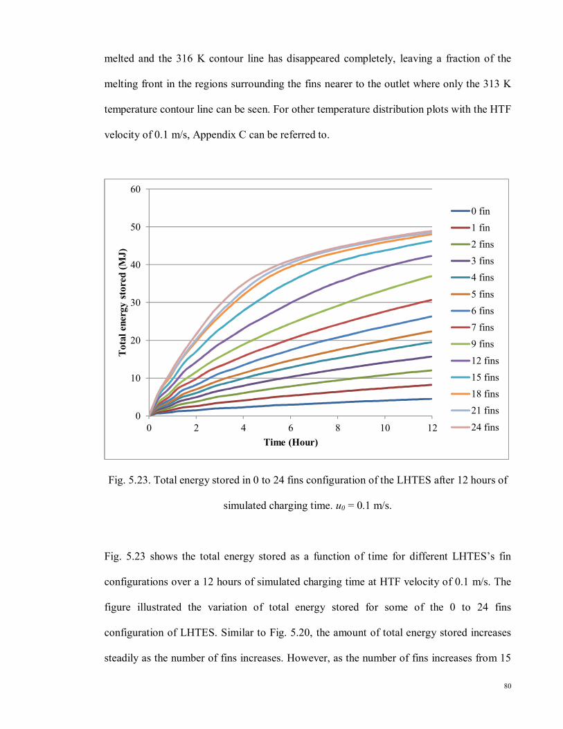
80

melted and the 316 K contour line has disappeared completely, leaving a fraction of the

melting front in the regions surrounding the fins nearer to the outlet where only the 313 K

temperature contour line can be seen. For other temperature distribution plots with the HTF

velocity of 0.1 m/s, Appendix C can be referred to.

Fig. 5.23. Total energy stored in 0 to 24 fins configuration of the LHTES after 12 hours of

simulated charging time. u0 = 0.1 m/s.

Fig. 5.23 shows the total energy stored as a function of time for different LHTES’s fin

configurations over a 12 hours of simulated charging time at HTF velocity of 0.1 m/s. The

figure illustrated the variation of total energy stored for some of the 0 to 24 fins

configuration of LHTES. Similar to Fig. 5.20, the amount of total energy stored increases

steadily as the number of fins increases. However, as the number of fins increases from 15

0

10

20

30

40

50

60

0 2 4 6 8 10 12

Tot

al e

ner

gy s

tore

d (

MJ

)

Time (Hour)

0 fin

1 fin

2 fins

3 fins

4 fins

5 fins

6 fins

7 fins

9 fins

12 fins

15 fins

18 fins

21 fins

24 fins

81

to 24 fins configuration, the rate of increase reduces significantly. As shown in Fig. 5.22,

almost all of the PCM volume has been melted into the liquid phase in the LHTES with

higher number of fins arrangement, reducing the latent thermal energy contribution to the

overall total energy stored. The minimum and maximum total energy stored according to

the results are 4.6 MJ and 48.9 MJ for 0 and 24 fins configurations respectively.

Fig. 5.24. Sensible and latent thermal energy stored in 0 to 24 fins configuration after 12

hours of simulated charging time. u0 = 0.1 m/s.

The chart shown in Fig. 5.24 illustrates the amount of sensible and latent thermal energy

stored in 0 to 24 fins configuration for HTF velocity of 0.1 m/s. The latent thermal energy

stored in the PCM shows a progressive increase from 2.1 MJ for 0 fin configuration to a

maximum of 31.1 MJ for 24 fins configuration. The rate of increase for sensible thermal

energy storage shows a progressive growth from 0 to 18 fins configuration, from which the

0

5

10

15

20

25

30

35

0 1 2 3 4 5 6 7 9 12 15 18 21 24

En

ergy

sto

red

(M

J)

Number of fins

Sensible Energy Latent Energy

82

increase rate seems to have slowed down as the number of fins increases. This is due to

most of the PCM has been melted as a result of the reduced PCM volume with increasing

number of fins.

5.5 LHTES maximum storage capacity and efficiency

As shown in the following Fig. 5.25, the plots for comparing between the maximum

possible energy storage capacities with actual energy stored in the PCM for various fins

configuration across the four different HTF velocities are presented. The maximum

capacity of energy stored in the PCM can be calculated by using the following equation in

which the whole PCM volume is assumed to be at the temperature of 350 K, which is the

inlet fluid temperature:

�� = �[(�� ∗ (313− 293)[1/�]) + (��,�� ∗ (316 − 313)[1/�])

The equation described in Eq. (5.6) is a COMSOL function which is used in the volume

integration of the PCM domain. In Fig. 5.25, the highest maximum energy storage capacity

that the entire PCM volume can store is 57.4 MJ for the 0 fin configuration. However, the

lowest maximum energy storage capacity is obtained for the LHTES with 24 fins

configuration with 52.3 MJ of possible thermal energy stored. The linear decrease of the

maximum storage capacity of the PCM shown in Fig. 5.25 is mainly due to gradual

reduction of the phase change material’s available volume. As the number of fins increases,

some of the phase change materials are displaced by the copper fins, reducing the possible

amount of energy that can be stored.

+(�� ∗ (350 − 316)[1/�])] (5.6)

83

Fig. 5.25. Total energy stored for various HTF velocities as compared to the maximum

storage capacity for 0 to 24 fins configuration of LHTES after simulated charging time of

12 hours.

The highest total energy that can be stored in the LHTES for the HTF of 0.05 and 0.1 m/s

velocities are 47.5 MJ and 48.9 MJ respectively in the 24 fins configuration LHTES. While

for HTF velocities of 0.01 and 0.03 m/s, their highest total energy stored is achieved in the

18 fins configuration with 38.9 MJ and 45.8 MJ respectively. The reason for the declining

of total energy increase rate as the number of fins increases from 18 to 24 fins, as shown in

Fig. 5.25 can be explained by referring to the melting fraction figure of Fig. 5.18 which

illustrates that almost all of the PCM has been melted starting with the 18 fins configuration

LHTES. Additionally, as expected the energy storage rate and the amount of melted PCM

of the low HTF velocity of 0.01 m/s is smaller than the other higher HTF velocities.

0

10

20

30

40

50

60

70

0 2 4 6 8 10 12 14 16 18 20 22 24

To

tal

ener

gy

sto

red

(M

J)

Number of fins

0.01 m/s

0.03 m/s

0.05 m/s

0.1 m/s

Maximumstoragecapacity

84

Fig. 5.26 shows the LHTES performance efficiency for some of the 0 to 24 fins

configuration for HTF of 0.01 m/s and 0.1 m/s velocities calculated by using the following

equation:

� =��

x100%

Fig. 5.26. Thermal energy storage efficiencies for various numbers of fins after 12 hours of

simulated charging time. HTF velocities: 0.01 m/s and 0.1 m/s.

As shown, the efficiency for both of the HTF velocities increases with the addition of fins.

The 0 fin configuration evidently has the lowest storage efficiencies having resulted to

achieve only about 7.5 and 7.9% efficiencies for HTF velocities of 0.01 and 0.1 m/s

respectively. Whereas, the highest recorded efficiency for both of the velocities is 93.5%

efficiency for 0.1 m/s in the 24 fins configuration LHTES and 72.7% efficiency for 0.01

m/s obtained in the 18 fins configuration.

0

10

20

30

40

50

60

70

80

90

100

0 2 4 6 8 10 12 14 16 18 20 22 24

Eff

icie

ncy

(%

)

Number of fins

0.01 m/s

0.1 m/s

(5.7)

85

Referring to Fig. 5.25, for the LHTES that uses HTF velocity of 0.01 m/s; the device

achieves the highest energy stored of 38.9 MJ with 18 fins configuration, which translates

to 72.7% of storage efficiency. Increasing the number of fins does not result in any increase

of total energy stored and storage efficiency, but the addition of fins shows that both plots

in Figs. 5.25 and 5.26 suffered reductions.

In LHTES device that uses HTF velocity of 0.1 m/s, the numerical results show a gradual

increase in total energy stored and storage efficiency. Furthermore, the addition of fins

from 18 to 24 shows that the rates of increase for both plots in Figs. 5.25 and 5.26 are

declining as the number of fins increases. Additionally, the total energy stored for 18 fins

configuration with HTF velocity of 0.1 m/s is 48.1 MJ which translates to 89.7% of storage

efficiency. Adding the total number of fins to 24 (33.33% increase), increases the total

energy stored by only 0.9 MJ, or 1.8% of increase.

Thus, from the discussion and results shown, a latent heat thermal energy storage device

with 18 fins configuration demonstrates a good balance between the storage performance

efficiency, the total thermal energy storage capacity and the cost of material needed to

manufacture the latent heat thermal energy storage system that uses paraffin wax as the

medium.

86

CHAPTER 6

CONCLUSION

6.1 Conclusion

The effective heat capacity method has been studied and showed that it can be used to

characterize the melting process of a phase change material. By using the modified heat

capacity that changes its value when the temperature of the PCM is in the melting range of

the paraffin wax (313K to 316K); the numerical problem of defining the non-linear

characteristic of PCM heat capacity can be solved. The modified heat capacity has been

incorporated successfully into the COMSOL software in order to study the effects of fins

and heat transfer fluid velocities on the thermal behavior of the PCM. On the other hand, a

slow heating zone (SHZ) was identified during the charging process. This area of the PCM

volume is slower to receive heat due to the gap between the fins and the container. The

higher thermal resistance of the SHZ area causes the PCM to melt slower which reduces the

melting fraction of the PCM.

The HTF velocities of 0.01, 0.03, 0.05 and 0.1 m/s were used in the numerical analysis of

LHTES for fin configurations of 0 to 24. After 12 hours of charging time, the sensible

energy stored in the solid and liquid phase of the PCM demonstrates a steady increase as

the HTF velocity increases. The results show that the minimum energy stored was recorded

for the 0 fin configuration and HTF velocity of 0.01 m/s with 2.37 MJ. Whereas, the

maximum sensible energy stored was achieved by the 24 fins configuration LHTES and

HTF velocity of 0.1 m/s with 17.84 MJ. The latent energy stored during the melting process

87

of the PCM shows a steady increase as the number of fins increases from 0 to 12 and also

across the various HTF velocities. However, the rate of increase of the latent energy stored

in the PCM from 15 to 24 fins configurations declines and appears to be constant for 0.03

m/s to 0.1 m/s HTF velocities. LHTES with 0.01 m/s HTF velocity however shows an

obvious reduction in latent heat contribution. This is caused by the increasing melted

fraction of the PCM volume as the number of fins increases. The minimum latent energy

stored was recorded for the 0 fin configuration and HTF velocity of 0.01 m/s with 1.97 MJ.

Whereas, the maximum latent energy stored was achieve by the 24 fins configuration

LHTES and HTF velocity of 0.1 m/s with 31.07 MJ. Overall, the effect of increasing HTF

velocities on the thermal behavior of the PCM shows that the amount of energy that can be

stored increases as the HTF velocity increases.

In the case pertaining to the effect of increasing the number of fins from 0 to 24 with HTF

velocities of 0.01 m/s and 0.1 m/s, generally the total energy that can be stored increases as

the number of fins increases. For the LHTES device that uses HTF velocity of 0.01 m/s, the

minimum energy stored was recorded for the 0 fin configuration with 4.33 MJ. Whereas,

the maximum energy stored was achieved for the 18 fin configuration LHTES with 38.93

MJ. The total energy stored in the higher number of fins shows a reduction due to the low

HTF velocity which in turn lowers the heat transfer rate to the PCM, congregating most of

the heat nearer to the inlet of the LHTES. Additionally, the minimum and maximum total

energy stored for HTF velocity of 0.1 m/s are 4.6 MJ and 48.9 MJ for 0 and 24 fins

configurations respectively.

The 0 fin configuration LHTES has the lowest storage efficiencies with only about 7.5 and

7.9% efficiencies for HTF velocities of 0.01 and 0.1 m/s respectively. The highest recorded

88

efficiency was recorded for the 24 fins configuration LHTES with 93.5% at HTF velocity

of 0.1 m/s. The highest efficiency for HTF velocity of 0.01 m/s was achieved by the 18 fins

configuration LHTES with 72.7%.

6.2 Recommendations

Future research studies may include the following recommendations:

1. The current study focuses only on the charging process of the PCM. Future studies

can include the discharging or solidification process of the PCM.

2. The current study assumes that the effects of free convection during the melting

process of the PCM are negligible. Further studies on employing free convection

during the charging process of the PCM using simpler geometry can be explored.

3. Other types of fin geometries can be further explored to study their effects on the

thermal behavior of the PCM.

4. The effects of fin thickness, height and gap between the fins and the container have

a good research values and can be further explored using COMSOL software.

5. Experimental works on the LHTES can be carried out in order to validate the

numerical analysis.

89

REFERENCES

ABHAT, A. 1983. Low temperature latent heat thermal energy storage: heat storage materials. Solar Energy, 30, 313-332.

ABHAT, A. et al., 1981. Development of a modular heat exchanger with an integrated latent heat storage. Report no. BMFT FBT 81-050. Germany Ministry of Science and Technology Bonn.

AGYENIM, F., HEWITT, N., EAMES, P. & SMYTH, M. 2010. A review of materials, heat transfer and phase change problem formulation for latent heat thermal energy storage systems (LHTESS). Renewable and Sustainable Energy Reviews, 14, 615-628.

AINSWORTH, M. & ODEN, J. T. 2000. A posteriori error estimation in finite element analysis, pure and applied mathematics. Wiley-Interscience.

ALEXIADES, V. & SOLOMON, A. D. 1992. Mathematical modeling of melting and freezing process. Washington, DC: Hemisphere Publishing Corporation.

ANICA, T. 2005. Experimental and numerical investigations of heat transfer during technical grade paraffin melting and solidification in a shell and tube latent thermal energy storage unit. Solar Energy, 79, 648-660.

AZPIAZU, M. N., MORQUILLAS, J. M. & VAZQUEZ, A. 2003. Heat recovery from a thermal energy storage based on the Ca(OH)2/CaO cycle. Applied Thermal Engineering, 23, 733-741.

BAYLIN, F. 1979. Low temperature thermal energy storage: a state of the art survey. Report no. SERI/RR/-54-164. Golden, Colorado, USA: Solar Energy Research Institute.

BECKETT, G., MACKENZIE, J. A. & ROBERTSON, M. L. 2001. A Moving Mesh Finite Element Method for the Solution of Two-Dimensional Stefan Problems. Journal of Computational Physics, 168, 500-518.

BENARD, C., GOBIN, G. & MARTINEZ, F. 1985. Melting in rectangular enclosures: experiments and numerical simulations. J Heat Transfer, 107, 794-802.

BENENSON, W., HARRIS, J. W. & STOCKER, H. 2000. Handbook of physics. New York: Springer-Verlag Inc.

BENLI, H. & DURMUS, A. 2009. Performance analysis of a latent heat storage system with phase change material for new designed solar collectors in greenhouse heating. Solar Energy, 83, 2109-2119.

BERTRAND, O., BINET, B., COMBEAU, H., COUTURIER, S., DELANNOY, Y., GOBIN, D., LACROIX, M., LE QUÉRÉ, P., MÉDALE, M., MENCINGER, J., SADAT, H. & VIEIRAF, G. 1999. Melting driven by natural convection. A comparison exercise: first results. Int J Therm Sci, 38, 5-26.

BINET, B. & LACROIX, M. 1998. Numerical study of natural-convection dominated melting inside uniformly and discretely heated rectangular cavities. Numer Heat Transfer Part A, 33, 207-224.

BISWAS, R. 1977. Thermal storage using sodium sulfate decahydrate and water. 99, 99-100.

BRENT, A. D., VOLLER, V. R. & REID, K. J. 1988. Enthalpy-porosity technique for modeling convection–diffusion phase change: application to the melting of a pure metal. Numer Heat Transfer, 13, 297-318.

90

BUDDHI, D. et al., 1988. Solar thermal storage systems using phase change materials. Int J Energy Res, 12, 547-555.

BUDDHI, D. & SAWHNEY, R. L. 1994. Proceedings on thermal energy storage and energy conversion, School of Energy and Environmental Studies, Devi Ahilya University, Indore, India.

CARSLAW, H. S. & JAGER, J. C. 1973. Conduction of heat in solids. Second ed. London: Oxford University Press.

CHARLSSON, B., STYMME, H. & WATTERMARK, G. 1979. An incongruent heat of fusion system CaCl26H2O made congruent through modification of chemical composition of the system. Solar Energy, 23, 333-350.

CHENG, W. L., MEI, B. J., LIU, Y. N., HUANG, Y. H. & YUAN, X. D. 2011. A novel household refrigerator with shape-stabilized PCM (Phase Change Material) heat storage condensers: An experimental investigation. Energy, 36, 5797-5804.

COMSOL 2011. COMSOL Multiphysics User's Guide. Version 4.2. DEBORAH, A. K. & MICHAEL, K. J. 2005. Introduction to thermal and fluid engineering.

New Jersey: John Wiley and Sons. DUTIL, Y., ROUSSE, D. R., SALAH, N. B., LASSUE, S. & ZALEWSKI, L. 2011. A

review on phase-change materials: Mathematical modeling and simulations. Renewable and Sustainable Energy Reviews, 15, 112-130.

ESEN, A. & KUTLUAY, S. 2004. A numerical solution of the Stefan problem with a Neumann-type boundary condition by enthalpy method. Applied Mathematics and Computation, 148, 321-329.

ETTOUNEY, H., ALATIQI, I., AL-SAHALI, M. & AL-HAJIRIE, K. 2006. Heat transfer enhancement in energy storage in sphericalcapsules filled with paraffin wax and metal beads. Energy Conversion and Management, 47, 211-228.

ETTOUNEY, H., EL-DESSOUKY, H. & AL-ALI, A. 2005. Heat transfer during phase change of paraffin wax stored in spherical shells. J Sol Energy Eng, 127, 357-366.

FARID, M. M. 1986. Solar energy storage with phase change. J Sol Energy Res, 4, 11-29. FARID, M. M., HAMAD, F. A. & ABU-ARABI, M. 1998. Phase change cool storage

using dimethyl-sulfoxide. Energy Conversion and Management, 39, 819-826. FARID, M. M. & HUSIAN, R. M. 1990. An electrical storage heater using phase change

method of heat storage. Energy Conversion and Management, 30, 219-230. FARID, M. M. & KANZAWA, A. 1989. Thermal performance of a heat storage module

using PCM’s with different melting temperatures: mathematical modeling. J Sol Energy Eng, 111, 152-157.

FARID, M. M., KIM, Y. & KANZAWA, A. 1990. Thermal performance of heat storage module using PCM’s with different melting temperatures: experimental. J Sol Energy Eng, 112, 125-131.

FLANDRO, G. A., MCMAHON, H. M. & ROACH, R. L. 2011. Basic aerodynamics: incompressible flow. Cambridge University Press.

FREUND, M., MÓZES, G. & JAKAB, E. 1982. Paraffin products: properties, technologies, applications. Amsterdam: Elsevier.

GARG, H. P., MULLICK, S. C. & BHARGAVA, A. K. 1985. Solar thermal energy storage, D. Reidel Publishing Co.

GEORGE, A. 1989. Hand book of thermal design. In: Guyer C, editor. Phase change thermal storage materials. McGraw Hill Book Co.

GHONEIM, A. A. 1989. Comparison of theoreticalmodels of phase-change and sensible heat storage for air and water-based solar heating systems. Solar Energy, 42, 209-220.

91

GO, Z., LIU, H. & LI, Y. 2004. Thermal energy recovery of air-conditioning system heat recovery system calculation and phase change material development. Applied Thermal Engineering, 24, 2511-2526.

GOODMAN, T. R. 1958. The heat balance integral and its application in problems involving a change. Trans ASME, 80, 335-342.

GROULX, D. & LACROIX, M. 2007. Study of the effect of convection on close contact melting of high Prandtl number substances. International Journal of Heat and Mass Transfer, 46, 213-220.

GROULX, D. & OGOH, W. 2009. Solid-liquid phase change simulation applied to a cylindrical latent heat energy storage system. Proceedings of the COMSOL Conference 2009.

GUPTA, S. C. 2003. The classical Stefan problem: Basic concepts, modelling and analysis.: Elsevier Science B.V.

HALAWA, E., BRUNO, F. & SAMAN, W. 2005. Numerical analysis of a PCM thermal storage system with varying wall temperature. Energy Conversion and Management, 46, 2592-2604.

HAMDAN, M. A. & ELWERR, F. A. 1996. Thermal energy storage using a phase change material. Solar Energy, 56, 183-189.

HASNAIN, S. 1998. Review on sustainable thermal energy storage technologies, Part I: heat storage materials and techniques. Energy Conservation and Management, 39, 1127-1138.

JIAN-YOU, L. 2008. Numerical and experimental investigation for heat transfer in triplex concentric tube with phase change material for thermal energy storage. Solar Energy, 82, 977-985.

JIJI, L. M. 2009a. Heat conduction. Third ed.: Springer-Verlag. JIJI, L. M. 2009b. Heat convection. Second ed.: Springer-Verlag. JONES, B. J., SUN, D., KRISHNAN, S. & GARIMELLA, S. V. 2006. Experimental and

numerical study of melting in a cylinder. international Journal of Heat and Mass Transfer, 49, 2724-2738.

KEUNG, C. S. 1980. The use of sources and sinks in solving two dimension conduction problem with change of phase in arbitrary domains. Ph.D. dissertation, Columbia University, New York.

KUZNIK, F., VIRGONE, J. & NOEL, J. 2008. Optimization of a phase change material wall-board for building use. Applied Thermal Engineering, 28, 1291-1298.

LACROIX, M. 1989. Computation of heat transfer during melting of a pure substance from an isothermal wall. Numer Heat Transfer Part B, 15, 191-210.

LACROIX, M. 2001. Contact melting of a phase change material inside a heated parallelepedic capsule. Energy Conversion and Management, 42, 35-44.

LACROIX, M. & BENMADDA, M. 1998. Analysis of natural convection melting from a heated wall with vertically oriented fins. Int J Numer Methods Heat Fluid Flow, 8, 465-478.

LACROIX, M. & VOLLER, V. R. 1990. Finite different solutions of solidification phase change problems: transformed versus fixed grids. Numer Heat Transfer Part B, 17, 25-41.

LAMBERG, P., LEHTINIEMI, R. & HENELL, A. M. 2004. Numerical and experimental investigation of melting and freezing processes in phase change material storage. International Journal of Thermal Sciences, 43, 277-87.

LAMBERG, P. & SIREN, K. 2003. Analytical model for melting in a semi-infinite PCM storage with an internal fin. Heat Mass Transf, 39, 167-176.

92

LANE, G. A. 1983. Solar heat storage-latent heat materials. Boca Raton, FL: CRC Press Inc.

LANE, G. A. et al., 1978. Macro-encapsulation of PCM. Report no. ORO/5117-8. Midland, Michigan: Dow Chemical Company.

LANE, G. A. & ROSSOW, H. E. 1976. Encapsulation of heat of fusion storage materials. In: Proceedings of the second south eastern conference on application of solar energy. 442-455.

LAUARDINI, V. J. 1981. Heat transfer in cold climates New York: Pub. Van Nostrand. LIU, C. & GROULX, D. 2011. Numerical study of the effect of fins on the natural

convection driven melting of phase change material. In: Proceedings of COMSOL conference. Boston.

LIU, Z. & CHUNG, D. D. L. 2005. Calorimetric evaluation of phase change materials use as thermal interface materials. Thermo Chemical Acta, 366, 135-147.

LIU, Z., SUN, X. & MA, C. 2005. Experimental study of the characteristics of solidification of stearic acid in an annulus and its thermal conductivity enhancement. Energy Conversion and Management, 46, 971-984.

MACKENZIE, J. A. & MEKWI, W. R. 2007. Adaptive computations: theory and algorithms. In: TANG, T. & XU, J. (eds.) On the use of moving mesh methods to solve PDEs. Beijing: Science Press.

MASSOUD, K. 2002. Principles of heat transfer. New York: John Wiley and Sons. MORISSON & ABDEL-KHALIK 1978. Effects of phase-change energy storage on the

performance of air-based and liquid-based solar heating systems. Solar Energy, 20, 57-67.

NATERER, G. F. 2003. Heat transfer in single and multiphase systems. Boca Raton, Florida: CRC Press LLC.

NAYAK, K. C., SAHA, S. K. & DUTTA, P. 2006. A numerical model for heat sinks with PCMs and thermal conductivity enhancers. international Journal of Heat and Mass Transfer, 49, 1833-1844.

PRAKASH, J., GARG, H. P. & DATTA, G. 1985. A solar water heater with a built-in latent heat storage. Energy Conversion and Management, 25, 51-56.

PROVATAS, N., GOLDENFELD, N. & DANTZIG, J. 1999. Adaptive mesh refinement computation of solidification microstructures using dynamic data structures. J Comput Phys, 148, 265-290.

REDDY, K. S. 2007. Thermal modeling of PCM-based solar integrated collector storage water heating system. J Sol Energy Eng, 129, 458-464.

REGIN, A. F., SOLANKI, S. C. & SAINI, J. S. 2008. Heat transfer characteristics of thermal energy storage system using PCM capsules: A review. Renewable and Sustainable Energy Reviews, 12, 2438-2458.

ROSEN, M. A. & DINCER, I. 2003. Energy methods for assessing and comparing thermal storage systems. International Journal of Energy Research, 27, 415-430.

SAITOH, T. S. & MOON, J. H. 1998. An experimental study for combined close-contact and natural convection melting in a spherical capsule. International Journal of Fluid Mechanics Research, 25, 220-229.

SAMAN, W., BRUNO, F. & HALAWA, E. 2005. Thermal performance of PCM thermal storage unit for a roof integrated solar heating system. Solar Energy, 78, 341-349.

SCHWARTZ, M. M. 2002. Encyclopedia of Materials, Parts, And Finishes. Second ed.: CRC Press.

93

SEENIRAJ, R. V., VELRAJ, R. & NARASIMHAN, N. L. 2002. Thermal analysis of a finned-tube LHTS module for a solar dynamic power system. Heat Mass Transf, 38, 409-417.

SHAMSUNDAR, N. & SPARROW, E. M. 1975. Analysis of multidimensional conduction phase change via the enthalpy model. J Heat Transfer, 97, 333-340.

SHAMSUNDAR, N. & SPARROW, E. M. 1976. Effect of density change on multidimensional conduction phase change. J Heat Transfer, 98, 550-557.

SHARMA, A., TYAGI, V. V., CHEN, C. R. & BUDDHI, D. 2009. Review on thermal energy storage with phase change materials and applications. Renewable and Sustainable Energy Reviews, 13, 318-345.

SHUKLA, A., BUDDHI, D. & SAWHNEY, R. L. 2009. Solar water heaters with phase change material thermal energy storage medium: a review. Renewable and Sustainable Energy Reviews, 13, 2119-2125.

SIMPSON, J. E. & GARIMELLA, S. V. 1998. An investigation of the solutal, thermal and flow fields in unidirectional alloy solidification. International Journal of Heat and Mass Transfer, 41, 2485-2502.

SPARROW, E. M. & HSU, C. F. 1981. Analysis of two-dimensional freezing on the outside of a coolant-carrying tube. International Journal of Heat and Mass Transfer, 24, 1345-1357.

STEFAN, J. 1891. Uber die theorie der eisbildung imbesondee uber die eisbindung im polarmeere. Ann. Phys. U. Chem., 42, 269-286.

STRITIH, U. 2004. An experimental study of enhanced heat transfer in rectangular PCM thermal storage. International Journal of Heat and Mass Transfer, 47, 2841-2847.

SUNA, D., ANNAPRAGADAB, S. R. & GARIMELLA, S. V. 2009. Experimental and numerical study of melting of particle-laden materials in a cylinder. International Journal of Heat and Mass Transfer, 52, 2966-2978.

SUWONDO, A., MANSOORI, G. & HIRAN, S. 1994. Characterization of alkanes and paraffin waxes for application as phase change energy storage medium. Energy Sources, 16, 117-128.

TAN, Z., LIM, K. M. & KHOO, B. C. 2007. An adaptive mesh redistribution method for the incompressible mixture flows using phase-field model. J Comput Phys, 225, 1137-1158.

TELKES, M. 1975. Thermal storage for solar heating and cooling. In: Proceedings of the workshop on solar energy storage sub-systems for heating and cooling of buildings. University of Virginia, Charlottesville.

TYAGI, V. V. & BUDDHI, D. 2007. PCM thermal storage in buildings: a state of art. Renewable and Sustainable Energy Reviews, 11, 1146-1166.

VOLLER, V. R. 1990. Fast implicit finite-difference method for the analysis of phase change problems. Numer Heat Transfer Part B, 17, 155-169.

WANG, Y., AMIRI, A. & VAFAI, K. 1999. An experimental investigation of the melting process in a rectangular enclosure. International Journal of Heat and Mass Transfer, 42, 3639-3642.

YEH, L. T. & CHUNG, B. T. 1975. Solidification and melting of material subjected to convection and radiation. J Space Cr Rockets, 12, 329-334.

ZALBA, B., MARIN, J. M., CABEZA, L. F. & MEHLING, H. 2003. Review on thermal energy storage with phase change: materials, heat transfer analysis and applications. Applied Thermal Engineering, 23, 251-283.

94

ZHANG, Y. & FAGHRI, A. 1996. Heat transfer enhancement in latent heat thermal energy storage system by using the internally finned tube. International Journal of Heat and Mass Transfer, 39, 3165-3173.

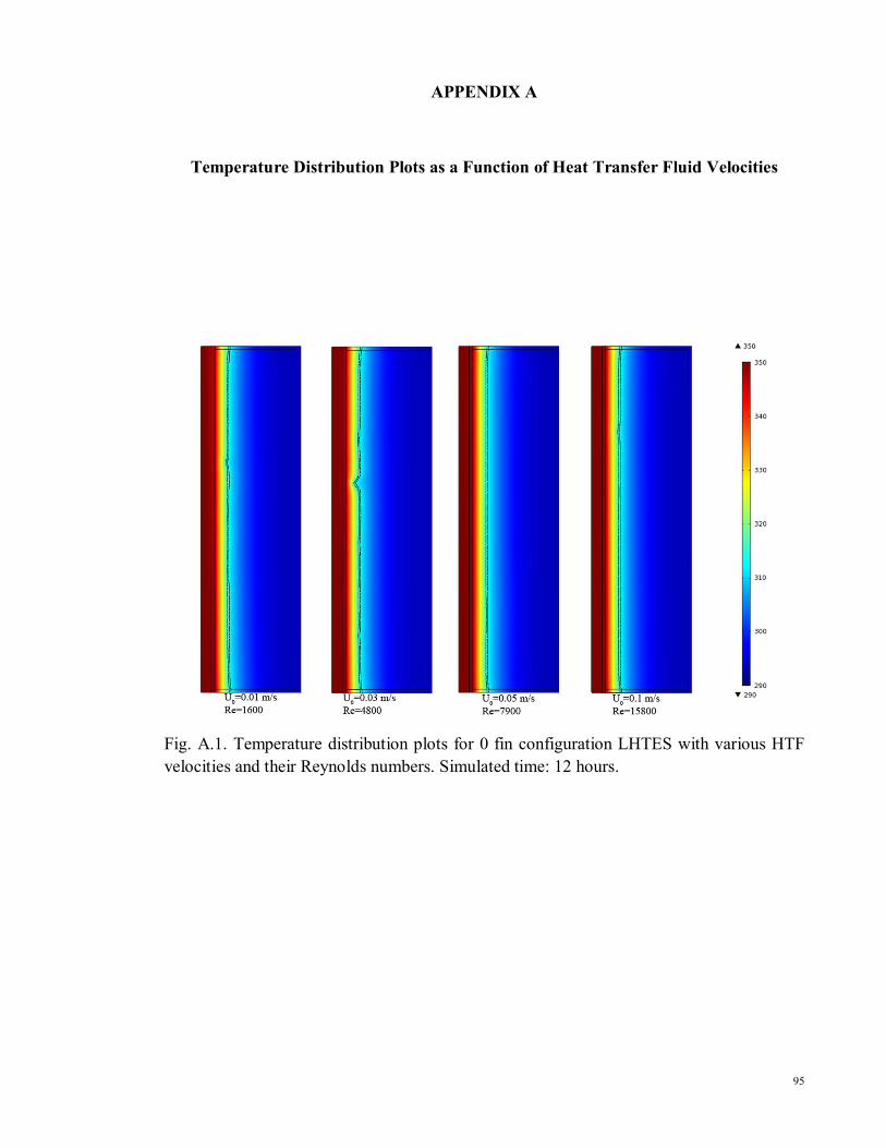
95

APPENDIX A

Temperature Distribution Plots as a Function of Heat Transfer Fluid Velocities

Fig. A.1. Temperature distribution plots for 0 fin configuration LHTES with various HTF

velocities and their Reynolds numbers. Simulated time: 12 hours.

96

Fig. A.2. Temperature distribution plots for 1 fin configuration LHTES with various HTF


Fig. A.3. Temperature distribution plots for 2 fins configuration LHTES with various HTF


97





98





99





100

Fig. A.10. Temperature distribution plots for 12 fins configuration LHTES with various




101





102



103

APPENDIX B

Temperature Distribution Plots as a Function of Number of Fins for HTF Velocity of

0.01 m/s

Fig. B.1. Temperature distribution plots for the 0, 1, 2, 3 and 4 fins configuration LHTES

after 12 hours of simulated charging time. u0=0.01 m/s.

104

Fig. B.2. Temperature distribution plots for the 5, 6, 7, 9 and 12 fins configuration LHTES


Fig. B.3. Temperature distribution plots for the 15, 18, 21 and 24 fins configuration LHTES


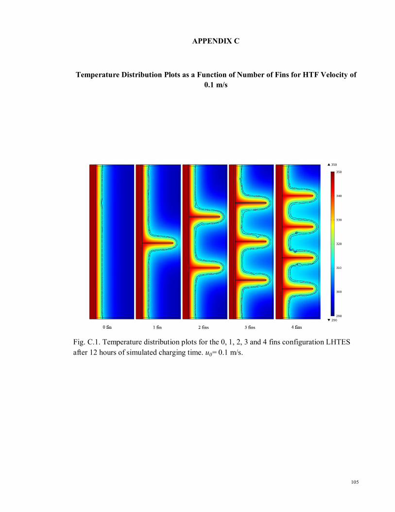
105

APPENDIX C

Temperature Distribution Plots as a Function of Number of Fins for HTF Velocity of

0.1 m/s

Fig. C.1. Temperature distribution plots for the 0, 1, 2, 3 and 4 fins configuration LHTES


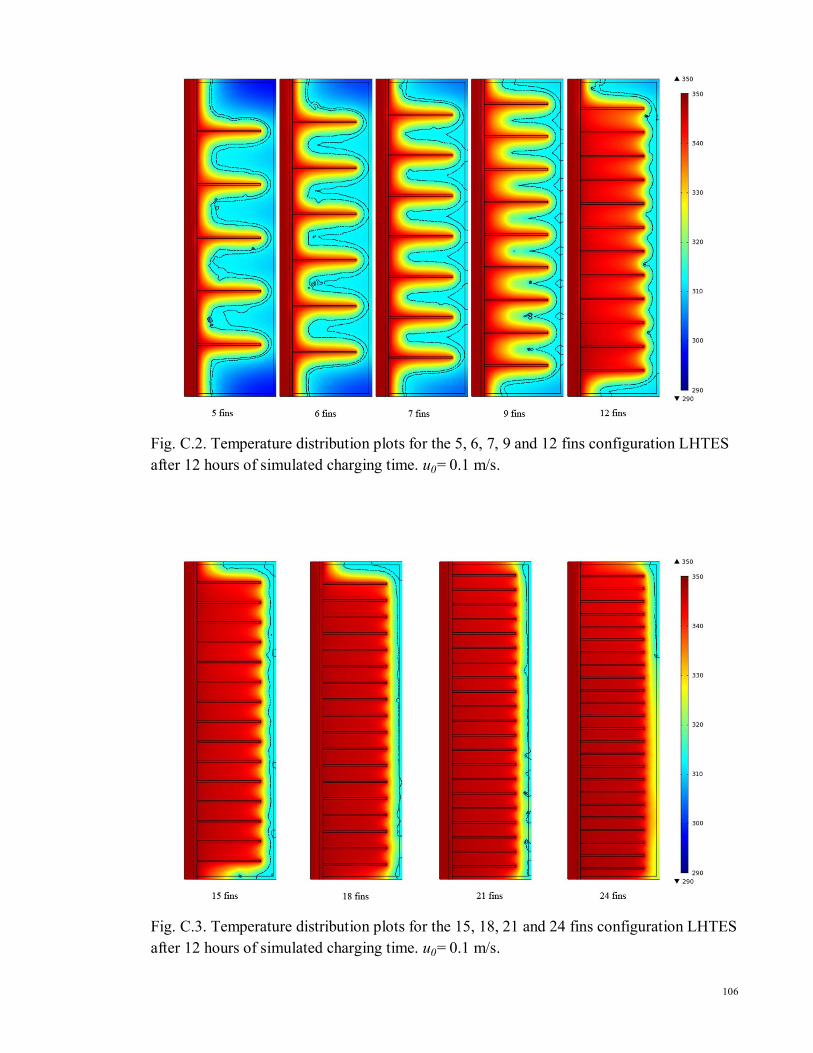
106

Fig. C.2. Temperature distribution plots for the 5, 6, 7, 9 and 12 fins configuration LHTES


Fig. C.3. Temperature distribution plots for the 15, 18, 21 and 24 fins configuration LHTES


numerical analysis of phase change material for...

Documents