numerical analysis of lamb waves using the finite and ... · because of the complexity of real...

INTERNATIONAL JOURNAL FOR NUMERICAL METHODS IN ENGINEERINGInt. J. Numer. Meth. Engng 2014; 99:26–53Published online 13 May 2014 in Wiley Online Library (wileyonlinelibrary.com). DOI: 10.1002/nme.4663

Numerical analysis of Lamb waves using the finite and spectralcell methods

S. Duczek1,*,† , M. Joulaian2, A. Düster2 and U. Gabbert1

1Otto von Guericke University Magdeburg, Universitätsplatz 2, 39106 Magdeburg, Germany2Hamburg University of Technology, Schwarzenbergstraße 95c, 21073 Hamburg, Germany

SUMMARY

An accurate and efficient simulation of wave propagation phenomena plays an important role in differentengineering disciplines. In structural health monitoring, for example, ultrasonic guided waves are used todetect and localize damage and to assess the structural integrity of the component part under consideration.Because of the complexity of real structures, the numerical simulation of structural health monitoringsystems is a computationally demanding task. Therefore, to facilitate the analysis of wave propagation phe-nomena, the authors propose to combine the finite cell method with the spectral element method. The ensuingnovel method is referred to as the spectral cell method. Because it does not rely on body-fitted meshes,the resulting approach eliminates all discretization difficulties encountered in conventional finite elementmethods. Moreover, with the aid of mass lumping, it paves the way for the use of explicit time-integrationalgorithms. In the first part of the paper, we show that using a lumped mass matrix instead of the consis-tent one has no detrimental effect on the accuracy of the spectral element method. We introduce the spectralcell method in the second part, showing that, when applied to wave propagation analysis, the spectral cellmethod yields results comparable with other standard higher order finite element approaches. Copyright ©2014 John Wiley & Sons, Ltd.

Received 18 February 2013; Revised 4 December 2013; Accepted 21 February 2014

KEY WORDS: p-FEM; SEM; FCM, SCM; fictitious domain method; Lamb waves; SHM

1. INTRODUCTION

A widely used and accepted technology in the structural health monitoring (SHM) of thin-walledstructures is to deploy the propagation of guided elastic waves for damage detection purposes [1–6].Named after their discoverer, Horace Lamb [7], they refer to elastic perturbations propagating inplate-like structures. Despite their complex characteristics, such as the occurrence of at least twodifferent modes for each frequency and the highly dispersive behavior [8], they are still a commonchoice for online monitoring systems [9–13]. Over the past few years, the focus of current researchactivities has shifted from simulating Lamb waves in relatively simple aluminum plates to morecomplex composites and sandwich panels [14–16]. Computing the wave propagation in these highlyheterogeneous structures is a fairly demanding task. Both the spatial and the temporal discretizationshave to be fine in order to resolve the high frequency at which Lamb waves are excited and to capturethe short wavelengths. To this end, we may take advantage of methods such as the h-version ofthe finite element method and the p-version of the finite element method (hierarchical higher orderFEM) [17–19], isogeometric analysis (IGA) [20], and the spectral element method (SEM) [21], toname just a few. The majority of applications of the p-FEM and the IGA have so far been in the formof research for static or eigenvalue problems [22–24]. Several articles have also dealt with fluid-

*Correspondence to: S. Duczek, Otto von Guericke University Magdeburg, Universitätsplatz 2, 39106 Magdeburg,Germany.

†E-mail: [email protected]

Copyright © 2014 John Wiley & Sons, Ltd.

LAMB WAVE ANALYSIS USING THE FCM AND THE SCM 27

structure interaction [25–28] using an implicit time-integration scheme. To the authors’ knowledge,these methods have not been extensively applied to wave propagation problems, because there hasnot been any viable algorithm for lumping the mass matrix in these methods so far. For this reason,implicit time-stepping algorithms are preferred, which makes the simulation very time consuming.Auricchio et al. published initial two-dimensional studies on explicit time-integration schemes forIGA based on a collocation approach [29]. Willberg et al. [30] studied the application of the p-FEMand the IGA for solving the elastic wave equation. This paper demonstrates that the convergencecharacteristics of all higher order C0-continuous finite element (FE) schemes are very similar. Theyalso showed that the use of higher order FEMs can mean significant savings in memory storagerequirements and numerical costs compared with commercially available FE-packages based onthe h-version.

Alternatively, the application of the SEM in this context is of great interest. The versatility of theSEM and its applications for wave propagation purposes have been shown by several authors [9, 21,31–43]. The widely accepted use of the SEM in dynamic problems is because it is easy to achievemass lumping, which allows us to take advantage of explicit time-integration algorithms efficiently.Dauksher and Emery [44, 45] demonstrated that a row-summing procedure employed to obtain adiagonal mass matrix can result in accurate solutions with spectral elements based on a Chebyshev–Gauss–Lobatto nodal distribution. This row-summing procedure is performed on the global massmatrix. Nonetheless, the solution characteristics are relatively unaffected by the diagonalized massmatrix, but the numerical costs for the solution of the equation system are drastically reduced whenapplying an explicit time-integration scheme. In this paper, we also pursue our investigations intothe effect of mass lumping on the accuracy of Lamb wave simulation when the SEM is employed.This is to ascertain that performing mass lumping techniques does not harm the accuracy. To thisend, we consider a benchmark example and investigate the convergence behavior of the method interms of the time of flight. We will demonstrate that the diagonalization of the mass matrix does nothave any detrimental effects on the accuracy of the SEM.

Unfortunately, despite their favorable numerical properties, it is not possible to recommend anyof the aforementioned approaches unreservedly. In the case of heterogeneous materials with a com-plex ‘micro’-structure, such as sandwich panels with a honeycomb core, the user is still faced withthe problem of mesh generation. It is widely known that generating conforming finite element gridsfrom complex computer-aided design-based (CAD-based) geometrical models involves quite exten-sive computational input as well as being very hard to automate completely, if it is at all possible. Theresulting mesh normally has to be adjusted manually by the user. In order to avoid such difficulties,the authors propose to take advantage of finite element-based approaches combined with fictitiousdomain methods [46–52] such as the recently proposed finite cell method (FCM) [53, 54]. The FCMdoes not call for body-fitted meshes but divides the domain into a Cartesian grid of rectangularcells. Thus, the geometric complexity does not cause any problems during the discretization pro-cess. The simple, yet effective idea behind this method is to extend the partial differential equationbeyond the physical domain of computation up to the boundaries of an embedding domain, whichcan be meshed without difficulty. The finite element mesh can accordingly be replaced by a grid ofstructured cells (Cartesian grid) embedding the whole domain. This offers hitherto undreamed ofpossibilities towards a holistic design approach. That is to say, the desired hexahedral meshes canbe generated on the basis of measurements given by X-ray tomography [53–56]. Applications of theFCM so far include the modal analysis of thin-walled structures [57], the homogenization of cellu-lar and foamed materials [55], multi-material problems [58], geometrically nonlinear problems [59,60], elasto-plasticity problems [61], damage mechanics [62], and bio-mechanics (numerical analysisof a femur bone e.g.) [63, 64], among others.

The main objective of this paper is to extend the FCM to structural dynamics for the simulationof elastic guided waves in thin-walled structures used in aerospace and automotive applications.Considering the popularity of the SEM in the wave propagation analysis community, we combine theideas of the SEM (employing spectral shape functions) with the fictitious domain concept. Our mainmotivations are

� taking advantage of higher order FEMs (accuracy, convergence rate, resilience to locking),

Copyright © 2014 John Wiley & Sons, Ltd. Int. J. Numer. Meth. Engng 2014; 99:26–53DOI: 10.1002/nme

28 S. DUCZEK ET AL.

� simplifying the discretization with the aid of a fictitious domain method,� exploiting the numerical advantages of explicit time-stepping schemes such as the central

difference method (CDM).

On the basis of the type of shape functions being used, we have coined the term spectral cell method(SCM) to describe the proposed approach. We chose the name in analogy to the differentiationbetween the finite element method and the spectral element method.

With the aforementioned objectives in mind, the layout for this paper is drafted as follows. Thesecond section briefly recalls the FEM and the SEM as well as investigating the viability of Lagrangeshape functions on a Gauss–Lobatto–Legendre (GLL) grid and studying the effect of different masslumping algorithms. The conclusions drawn from this section are important for the successful appli-cation of the SCM to wave propagation analysis. This is also the point of departure for derivingthe SCM in the next section. Thereafter, the third section features the basic principles of the FCMand its extension to the SCM. Only novel assumptions deviating from the standard FEM approachare discussed here. The fourth section deals with their application to a simple, two-dimensionalwave propagation problem in a perturbed structure and a more complex three-dimensional exam-ple involving a plate with a conical hole. The last section of the paper contains a conclusion and anoutlook on ongoing research.

2. THE FINITE AND THE SPECTRAL ELEMENT METHOD

The following section briefly recalls the fundamentals of the FEM and the SEM, which differ onlyin the choice of ansatz functions. All fundamental principles are identical, so we do not endeavor todifferentiate between those methods based on the shape functions.

2.1. Finite element method

The finite element developments are based on the variational formulation corresponding to Navier’sequations, namely Hamilton’s principle. It states that the motion of the system within the timeinterval Œt1; t2� is such that, under infinitesimal variations of the displacements, the Hamiltonianaction SH vanishes, meaning that the motion of the system follows the path of the stationaryaction [65]

ıSH D ı

t2Zt1

.LCWE / dt D 0 : (1)

Here L represents the Lagrangian function, and WE the work performed by the external forces.The Lagrangian is the difference between the kinetic energy K and the elastic strain energy WI(L D K �WI ). After some calculations and the substitution of Hooke’s law into Equation (1), thevariational formulation takes the following form:

0 D �

Z�

��ıuT RuC ı"TC"

�d�

„ ƒ‚ …ıL

C

Z�

ıuTFV d�CZ�

ıuTFS d�

„ ƒ‚ …ıWE

; (2)

where � is the mass density, " and � are the vectors of mechanical strains and stresses in Voigtnotation, respectively [66]. C denotes the elasticity matrix, and Ru represents the acceleration vector.The external forces can be divided into surface loads FS and volume loads FV .� and � represent thecomputational domain and its boundary, respectively. If we divide the domain of interest into severalelements, then the displacement field u.x; t / in each finite element, denoted by e, is approximatedby the product of the space-dependent shape function matrix Ne.x/ and a time-dependent vector ofunknowns Ue.t/,

u.x; t / D Ne.x/Ue.t/: (3)



The mechanical strain is defined as

" D DNeUe D BeUe; (4)

by introducing the strain-displacement matrix as Be D DNe , where D is a linear differentialoperator relating strains and displacements. With the aid of Equations (2), (3), and (4) and thereasoning that Hamilton’s principle has to be satisfied for all variations ıue D Ne ıUe , we obtainthe well-known equations of motion

MgRUg CKgUg D fg ; (5)

where the system matrices are obtained by assembling all element matrices

Mg DneAeD1

Me; (6)

Kg DneAeD1

Ke; (7)

fg DneAeD1

fe: (8)

The elemental mass and stiffness matrix as well as the elemental load vector are given as

Me D

Z�e

�NTe Ned�; (9)

Ke D

Z�e

BTeCBed�; (10)

fe DZ�e

NTe FeV d�CZ�e

NTe FeSd�; (11)

where �e and �e are the elemental domain and its corresponding boundary. For further explana-tions, such as including the influence of damping in the FEM, the reader should refer to standardtextbooks on this subject by Zienkiewicz and Taylor [66–68], Wriggers [69], Bathe [70], Fish andBelytschko [71], and Hughes [72], for instance.

2.2. Spectral element method

The selection of the shape functions in Equation (3) plays a key role in the accuracy and efficiency ofthe finite element approach. In the SEM, shape functions are defined on the basis of a set of Lagrangepolynomials utilizing a specific (non-equidistant) nodal distribution on the interval Œ�1;C1�. The.p C 1/ one-dimensional basis functions are formally defined by

N Lagrange; pn .�/ D

pC1YjD1; j¤n

� � �j

�n � �j; n D 1; 2; : : : ; p C 1: (12)

The nodal distribution �j with j D 1; : : : ; .pC1/ that is applied in the current article is defined as

�j D

8<:�1 if j D 1;

�Lo;p�10;j�1 if 2 6 j < p C 1;C1 if j D p C 1;

(13)


30 S. DUCZEK ET AL.

where �Lo;p�10;a with a D 1; : : : ; .p�1/ denotes the roots of the .p�1/th-order Lobatto polynomial

Lop�1.�/ D1

2ppŠ

dpC1

d�pC1

h��2 � 1

�pi: (14)

This nodal distribution is generally referred to as a GLL grid. Spectral elements employing the GLLgrid have been proposed by Komatitsch and Tromp [43], Cohen [73], Zak et al. [74], Kudela et al.[75], Peng et al. [39], and Ha and Chang [76], to mention just a few.

2.2.1. Temporal discretization. Equation (5) needs to be discretized in time, too. There are differentschemes available for this purpose. We can employ either implicit or explicit time-integration algo-rithms. Because we use ultrasonic guided waves in our research activities in SHM to detect andidentify flaws in typical thin-walled engineering structures that are in the order of millimeter (mm),high frequencies in the kilohertz–megahertz (kHz-MHz) range are required. This requires a very finespatial and temporal discretization. For this kind of simulation (wave propagation), explicit methodsare of great interest. Although several unconditionally stable implicit algorithms exist, it is not pos-sible to choose a time-step size that is significantly bigger than for explicit methods. There are twomain reasons that confirm this statement. First of all, the physics of the problem requires time-stepsizes that are comparable with the critical time-step size of explicit methods. Moreover, Dauksherand Emery [44] have shown that under certain circumstances, explicit methods are comparable withimplicit methods in terms of accuracy. Generally speaking, the time-step size should be selected insuch a way that the wave does not travel one element width in one time step. This corresponds toadhering to the Courant–Friedrich–Levy condition

�t Dbe

cgr: (15)

For typical guided wave propagation analysis, the element size be is in the range of a fewmillimeters, and the group velocity is between cgr � 2900 m/s and 5414 m/s (material propertiesof aluminum, cf. Table I). Accordingly, the time-step �t should be less than approximately 10�8 s.This is within the range of an explicit time-integration scheme. Therefore, it is advisable to applyexplicit time-integration schemes for our purpose.

2.2.2. Mass lumping procedures for the spectral element method. In order to increase the compu-tational efficiency of explicit time-integration schemes such as the central difference method, masslumping techniques are essential. In the course of this section, we show that mass lumped spectralelements offer significant advantages over the consistent mass formulation in terms of computa-tional efficiency. Keeping that in mind, there are two straightforward mass lumping possibilities thatare required for spectral elements, in order to benefit from explicit time-marching algorithms,

� mass lumping using the so-called GLL quadrature,� mass lumping based on a simple diagonalization technique such as the row-summing proce-

dure.

Other more elaborate methods (dual ansatz functions, for instance) are not included in the study.Because the spectral elements are developed on the basis of a GLL grid, using the GLL quadraturerule proves a neat way of diagonalizing the mass matrix [43, 74, 77]. This lumping procedure allowssubstantial savings in computational time if an explicit time-integration scheme is used, while muchless memory is required to save the inverted mass matrix. In addition, in the case of a mesh withundistorted elements, the diagonalization also minimizes the round-off errors, as shown in [77].

Table I. Material data for aluminum.

Young’s Poisson’s Mass Longitudinal Transversalmodulus (E) ratio (�) density(�) speed (c1) speed (c2)

7 � 1010 N/m2 0:33 2700 kg/m3 6197 m/s 3121 m/s



Alternatively, as shown in [45], a row-summing procedure can also result in accurate solutionswith spectral elements. The row-summing procedure is performed on the global mass matrix and isdefined as

Mlumpedii D

ndofXjD1

Mij ; Mlumpedij D 0 for i ¤ j: (16)

Dauksher and Emery [44, 45] have shown that the solution characteristics of spectral elements basedon a Chebyshev grid are relatively unaffected by the diagonalization, that an increased polynomialorder moderates the effects of lumping, and that no negative diagonal terms are generated. Theseproperties are also valid for spectral elements based on a GLL grid, as will be shown in the followingsection. The authors also claim that the results they obtained indicate that explicit spectral solutionsrequire fewer nodes per wavelength than needed by comparable consistent mass matrix solutions fora given accuracy [44]. This means that the mathematically correct consistent mass formulation mayyield less accurate solutions for the acoustic wave equation than either the empirical row-summingor the GLL quadrature formulations. This statement has to be investigated in detail but initial results(cf. Section 2.2.3) point to it being valid. In the remainder of the paper, we will distinguish betweennodes and modes per wavelength. It is only in the case of the SEM/SCM that nodes have a physicalinterpretation, otherwise they are referred to as modes because they only describe the unknownsconnected to the shape functions (p-FEM/FCM).

2.2.3. Evaluation of the different mass lumping procedures. The subsequent convergence studyis chosen to investigate the influence of different mass lumping techniques on the quality of thenumerical simulation of Lamb waves.

Benchmark problem—setup. Let us consider a two-dimensional plane strain model. Physicaldamping is not included, as it does not influence the convergence behavior. The geometry and theboundary conditions are depicted in Figure 1.

The length of the aluminum plate is given as lp D 500 mm and the thickness as d D 2 mm. Thematerial properties are summarized in Table I. The length of the plate guarantees that no reflectionfrom the right-hand boundary affects the signals at the points of measurement during the simulationtime (‘infinite’ plate assumption). Lamb waves are normally excited using distributed loads (exertedby piezoelectric transducers) on the top surface of the plate. In the two-dimensional model (cf.Figure 1), this load is modeled as a distributed load acting in the x2-direction (cf. Figure 3). Itstime-dependent amplitude follows a sine burst signal given by

F.t/ D OF sin!t sin2�!t

2n

�; 0 6 t 6 n

f; (17)

where ! D 2f denotes the central circular frequency. This kind of pulse has the advantage thatthe frequency content is narrow banded, cf. Figure 2. The number of cycles n within the signal

Figure 1. Two-dimensional model with loads and boundary conditions for the convergence study (symmet-ric boundary conditions at x1 D 0). We apply a surface load with a time-dependent amplitude F.t/ to thestructure. For the sake of simplicity, the surface load is indicated by a point force in the figure. The dimen-sions of the aluminum plate (Table I for material properties) are as follows: la D 100 mm, lb D 200 mm,

lp D 500 mm, and d D 2 mm.


32 S. DUCZEK ET AL.

Figure 2. Sine-burst. (a) Time domain signal. (b) Frequency content.

Figure 3. Concentrated point force Fres.t/ modeled as an equivalent constant traction T.t/ (symmetricmodel). According to Saint-Venant’s principle, both loads are equivalent with respect to their impact on the

displacement field.

determines the width of the excited frequency band around the central frequency f . We choose anexcitation frequency of f D 250 kHz, and the excitation signal contains 5 cycles (n D 5).

Generally speaking, the excitation by concentrated forces is inadmissible, because it might leadto solutions with infinite strain energies [17]. Accordingly, a traction T.t/, acting on the surface �of the structure (cf. Figure 3), is preferred and generally recommended. Using this procedure, weapply a consistent load to the model without introducing a singularity. In a two-dimensional setting,the proposed approach is given by

Fres.t/ DZ�

T.t/ d�: (18)

Considering a structured mesh employing rectangular finite elements and a constant distributedsurface load (cf. Figure 3), Equation (18) reduces to

Fres.t/ D T.t/ � be: (19)



Here be denotes the width of the finite element chosen for the load implementation. For the currentexample, the size of the first finite element has been reduced to be D 1 mm.

Symmetry boundary conditions are applied to the left-hand boundary (x1=0) of the model in orderto exploit the symmetry of the problem (cf. Figure 3). For the sake of the convergence study, wesave the time history of the displacement field at the location of the two points A (uA) and B (uB )on the top surface; see Figure 1.

Benchmark problem—evaluation of the accuracy of the results. The time of flight tc of the propa-gating Lamb wave packet between the points A and B (Figure 4) is used to determine the quality ofthe numerical solution [31].

The time of flight computed with the help of the SEM (tcSEM ) is compared with the valueobtained by a numerical ‘overkill’ solution (tcref ) on the basis of the p-version of the FEM(discretization: px1 D px2 D 8, nx1 D 1000, nx2 D 4, ndof D 528; 066, �t D 2:2 � 10�9 s).In order to extract this value from the finite element or reference solution, the time signal of thedisplacement at the relevant point (A or B) is subjected to a Hilbert transform [78, 79]

HA;B.u.t// D1

1Z�1

uA;B./ �1

t � d: (20)

Using the Hilbert transform HA;B of the time-dependent signal uA;B , it is possible to compute theenvelope eA;B of the time-displacement history. The time of flight is then evaluated by comparingthe position of the centroid of the envelope of the time signal at these two points. The envelope canbe calculated by means of the following relation

eA;B.t/ D

qHA;B.uA;B.t//2 C uA;B.t/2; (21)

and the coordinate of its centroid is obtained by determining the statical moment of the envelope

tA;B D

tendR0

eA;B.t/ � t dt

tendR0

eA;B.t/ dt

: (22)

Finally, the time of flight is computed as

tc D tB � tA : (23)

Basically speaking, using this methodology, the comparison of the time of flights equals theevaluation of the resulting group velocities (if the fundamental modes are well separated), becausedispersive effects are almost excluded due to both the narrow bandwidth of the excitation signal andthe constant distance between the evaluation points [80]. However, the remaining small dispersive

Figure 4. Time of flight as the difference between the centroid of two Hilbert envelopes at points A and B.


34 S. DUCZEK ET AL.

Figure 5. Area beneath the envelope of the displacement signal�uA;mag D

qu21;AC u2

2;A

at point A.

effects influence both calculated time of flight values, tcref and tcSEM , to an equal extent, so theconvergence indicator presented here is able to quantify the Lamb wave behavior even for very loworders of the error’s magnitude.

By way of a second measure, the area beneath the envelope of the signal at point A (uA;mag—magnitude of the displacements at point A) is computed and again compared with the referencevalue (cf. Figure 5). This indicates whether the amplitude is accurate within the simulation interval

Au D

Zt

uA;mag.t/dt: (24)

Benchmark problem—convergence study. For the current investigation, the polynomial degree inx2-direction is set to px2 D 6 for all of the computations to ensure a good spatial resolution withone element in x2-direction only [30]. We then proceed to investigate the convergence behavior ofspectral elements for several polynomial degrees (px1 D 2; 3; : : : ; 6) and different element sizesin x1-direction. To assess the accuracy of the solutions, we plot the relative error in the time of flightand the area against the number of nodes per (anti-symmetric) wavelength �A0 (cf. Figures 6 and7). The value of �A0 , for a given model discretized with a regular mesh, is determined using

�A0 Ddegrees of freedom

2.px2 C 1/lp� �A0 : (25)

px2 denotes the polynomial degree in x2-direction, lp is the length of the plate, and �A0 expressesthe wavelength of the anti-symmetric Lamb wave mode. Because the anti-symmetric mode has ashorter wavelength, it is the more critical mode from a modeling point of view. The relative error istherefore determined by comparing the numerical solution with the reference solution. This can beexpressed as

Erel Daref � anum

aref� 100 Œ%�: (26)

In this case, a depicts either the time of flight tc or the area beneath the envelope of the timesignal Au.

Figures 6 and 7 display the results of the convergence studies. An almost constant error plateauis reached at approximately 0:01% to 0:001% meaning that the results are very accurate. Furtheraccuracy can be obtained by refining the spatial resolution in x2-direction and choosing a smallertime-step size. Willberg et al. [30] showed that commercial tools based on the h-version of the FEMare unable to attain that level of accuracy.

We can see that the results of the aforementioned lumping techniques virtually coincide. Thereis no noticeable difference between the convergence behavior of the different numerical approachesfor diagonalizing the mass matrix in the SEM. These results also confirm the findings of Dauksher



Figure 6. Convergence curve for the wave propagation in an aluminum plate (relative error in time of flighttc)—on the basis of a numerical “overkill” solution (px1 D px2 D 8, nx1 D 1000, nx2 D 4, ndof D

528; 066). (a) px1=2; (b) px1 D 3; (c) px1 D 4; (d) px1 D 5; and (e) px1 D 6.

and Emery [44, 45] and highlight the fact that both lumping techniques essentially produce the sameresults. The results illustrate that increasing the polynomial order moderates the effects of masslumping and that no negative diagonal terms are produced. Moreover, increasing the polynomialdegree of the shape functions is a very efficient way of reducing the relative error. The curvesfeature peaks that can be attributed to internal element eigenfrequencies excited by the travelingwave packets [81].

3. THE FINITE AND SPECTRAL CELL METHOD

This section briefly introduces the concept of the finite cell method (FCM) and combines it with thespectral element method (SEM), calling the resulting approach spectral cell method (SCM). For adetailed discussion of the basic idea of the FCM, the reader should refer to [53–55, 63]. Because the


36 S. DUCZEK ET AL.

Figure 7. Convergence curve for the wave propagation in an aluminum plate (relative error in area Au)—onthe basis of a numerical “overkill” solution

�px1 D px2 D 8; nx1 D 1000; nx2 D 4; ndof D 528; 066

�.

(a) px1 D 2; (b) px1 D 3; (c)px1 D 4; (d)px1 D 5; and (e)px1 D 6.

SCM approach is very similar to the SEM, the main differences are highlighted only. By introducingspectral shape functions into the fictitious domain concept, we expect to be able to exploit theadvantages of an explicit time-marching algorithm, such as the CDM. Bearing the efficiency of thesolver in mind, however, it is essential to have the means of diagonalizing the mass matrix of thechosen approach.

3.1. The fictitious domain concept

As depicted in Figure 8, the physical domain �, on which the problem to be solved is definedin terms of a variational formulation, is embedded in a fictitious domain �f ict resulting in theembedding domain�ed . The variational principle describing linear elastic problems, whether staticor dynamic, is the same as for the standard FEM, see Section 2.1, so we refrain from repeating thebasic equations of elasto-dynamics at this point.



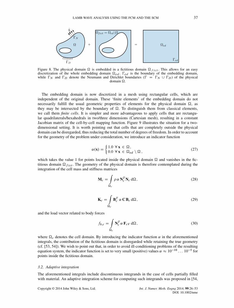
Figure 8. The physical domain � is embedded in a fictitious domain �f ict . This allows for an easydiscretization of the whole embedding domain �ed . �ed is the boundary of the embedding domain,while �N and �D denote the Neumann and Dirichlet boundaries (� D �N [ �D) of the physical

domain �.

The embedding domain is now discretized in a mesh using rectangular cells, which areindependent of the original domain. These ‘finite elements’ of the embedding domain do notnecessarily fulfill the usual geometric properties of elements for the physical domain �, asthey may be intersected by the boundary of �. To distinguish them from classical elements,we call them finite cells. It is simpler and more advantageous to apply cells that are rectangu-lar quadrilaterals/hexahedrals in two/three dimensions (Cartesian mesh), resulting in a constantJacobian matrix of the cell-by-cell mapping function. Figure 9 illustrates the situation for a two-dimensional setting. It is worth pointing out that cells that are completely outside the physicaldomain can be disregarded, thus reducing the total number of degrees of freedom. In order to accountfor the geometry of the problem under consideration, we introduce an indicator function

˛.x/ D²1:0 8 x 2 �;0:0 8 x 2 �ed n� ;

(27)

which takes the value 1 for points located inside the physical domain � and vanishes in the fic-titious domain �f ict . The geometry of the physical domain is therefore contemplated during theintegration of the cell mass and stiffness matrices

Mc D

Z�c

� ˛NTc Nc d�; (28)

Kc D

Z�c

BTc ˛C Bc d�; (29)

and the load vector related to body forces

fb;c D

Z�c

NTc ˛ FcV d�; (30)

where �c denotes the cell domain. By introducing the indicator function ˛ in the aforementionedintegrals, the contribution of the fictitious domain is disregarded while retaining the true geometry(cf. [53, 54]). We wish to point out that, in order to avoid ill-conditioning problems of the resultingequation system, the indicator function is set to very small (positive) values ˛ � 10�10 : : : 10�5 forpoints inside the fictitious domain.

3.2. Adaptive integration

The aforementioned integrals include discontinuous integrands in the case of cells partially filledwith material. An adaptive integration scheme for computing such integrands was proposed in [54,


38 S. DUCZEK ET AL.

Figure 9. Finite cell discretization. To control the influence of the fictitious domain on the accuracy of theresults, we introduce an indicator function ˛.

Figure 10. Sub-cells for the adaptive integration scheme. The original finite cell is refined if it is cutby the boundary of the physical domain. Several refinement levels are required to resolve the boundarysatisfactorily. This is checked by computing the area of the domain of interest. The refinement process is

stopped once a certain relative error is reached.

82]. Figure 10 depicts a schematic sketch of the integration technique employed. The Gaussianquadrature assumes that the integrands are smooth, an assumption that is violated by introducingthe indicator function ˛ within the finite cells. The FCM consequently uses a composed Gaus-sian quadrature to improve the integration accuracy in cells cut by geometric boundaries (cutcells). For integration purposes, the original cells are divided into a set of sub-cells by means of aquadtree/octree space-partitioning scheme [53, 82]. Several refinement levels are required to ensurea sufficient accuracy. Starting with the original finite cell of level k D 0, the algorithm first checkseach sub-cell of level k D i to see whether it is cut by a geometric boundary. If so, the relevant cellis replaced by 4/8 equally spaced sub-cells of level k D i C 1 in 2D/3D. In Figure 10, the corre-sponding finite cell is plotted in black, whereas the sub-cells used for integration purposes only areindicated by brighter lines. To increase the efficiency of the adaptive quadrature scheme, it is alsopossible to adjust the number of integration points for each individual sub-cell [83].

Because the boundary of the physical domain will not normally coincide with the boundary ofthe cells, special care has to be taken when considering the application of boundary conditions. The



treatment of Neumann boundary conditions is discussed in [54]. With regard to the application ofDirichlet boundary conditions, we recommend Nitsche’s method [84], which was employed for theFCM in [63].

According to the findings made in Section 2.2.3, it is still possible to reach a reasonable accuracyin simulating Lamb waves by the SEM employing mass lumping techniques. In the case of theSCM, for the sake of efficiency, we are also interested in employing such techniques. With theSCM, those cells that are completely filled with material can be lumped without any difficultieseither by performing row-summing technique or employing the GLL quadrature. In the case of cutcells, the adaptive element integration can be performed accurately by applying a Gauss–Legendrequadrature. As far as the mass lumping is concerned, it remains to be seen whether the row-summingtechnique can also be employed for the cut cells.

4. NUMERICAL VERIFICATION

This section demonstrates the capabilities of the finite cell method and the spectral cell method.The purpose is to resolve important wave propagation characteristics, such as the multi-modalbehavior of Lamb waves, as well as their dispersive nature. To this end, we begin by choosing asimple two-dimensional benchmark problem with a circular hole. This academic problem can beregarded as a proof of concept for the FCM/SCM methodology with respect to wave propagationanalysis. By way of a second example, the approach is extended to three dimensions. The modelconstitutes a three-dimensional plate perforated by a conical hole. We conduct a convergence studybased on a p-refinement for the three-dimensional model comparing the performance of the FCM,the SCM, and the SEM. In reference [85] we provide a detailed study of the convergence propertiesof the SCM and the application of different mass lumping techniques.

4.1. Two-dimensional perforated plate

The benchmark problem is a two-dimensional plate with a circular hole. The hole is located eccen-trically from the mid-plane of the structure (cf. Figure 11). This geometric perturbation causes modeconversion and thus highlights an important characteristic of Lamb waves [10].

Figure 11. The 2D aluminum plate (E D 70; 000N=mm2; � D 0:33, � D 2700 kg=m3) with a circularhole (not to scale). Loads and boundary conditions are marked in the figure. Two surface loads F1.t/ andF2.t/ D aF1.t/ are applied, with a D 1 for the excitation of a purely symmetric Lamb wave mode (S0) anda D �1 if the anti-symmetric mode (A0) is considered. For the sake of simplicity, they are only indicated asconcentrated loads. The dimensions of the plate are as follows: l1 D 100 mm, l2 D 50 mm, l3 D 152 mm,lp D 600 mm, tp D 5 mm, d D 2 mm, and e D 2 mm. The signal parameters are as follows: OF D 1N ,

! D 2f , f D 200 kHz, and n D 5.

Figure 12. Contour plots of the traveling waves in an aluminum plate with a circular hole highlighting theeffect of mode conversion at anti-symmetrical perturbations of the structure under investigation. (a) Incident

S0 wave packet; and (b) converted A0- and transmitted S0-modes.


40 S. DUCZEK ET AL.

The areas marked with a red (solid line) and a blue (dashed line) rectangle, respectively,(approximately) indicate the position of the contour plots of the traveling wave depicted in Figure 12.A pure S0-mode is excited on the left-hand boundary of the plate (cf. Figure 12(a)). Some distanceaway from the local perturbation, we clearly see that a converted A0-mode occurred in addition tothe transmitted S0-wave packet (cf. Figure 12(b)). The location of the contour plot is chosen in sucha way that the faster S0-mode is clearly separated from the A0-mode.

For the sake of minimizing the numerical costs, we assume infinite dimensions in x3-directionand subsequently utilize the plane strain assumption. This poses no limitation to the results obtained,as all key features of guided wave propagation can be studied using this setup. The boundary con-ditions, material properties, and the dimensions of the plate are given in Figure 11. The history ofthe displacement field is saved at the measurement points P1 to P4. The results obtained using theFCM and the SCM are later compared with reference solutions attained by applying the p-versionof FEM.

4.1.1. Model setup. The ultrasonic guided waves are excited using a pair of collocated surface loadson the top and the bottom of the plate (cf. Figure 11). They act in x2-direction, and their time-dependent amplitudes follow a sine burst signal. For the sake of clarity, we repeat the formula at thispoint (cf. Equation (17)),

F.t/ D OF sin!t sin2�!t

2n

�; 0 6 t 6 n

f:

Applying these loads to the top and bottom surfaces allows us to exploit the advantages of a mono-modal excitation, which means that only a single mode is present at a time for f � tp < 1:5MHzmm(cf. Figure 13). In order to generate a signal containing only the A0-mode, both forces have to act

Figure 13. Dispersion diagram for aluminum�E D 70; 000 N=mm2; � D 0:33

. (a) Group velocity; and

(b) phase velocity.



in the same direction, meaning they have to be in phase. If the two loads are out of phase, a pureS0-mode is generated.

The rest of this section is dedicated to explaining how to choose the discretization parameterand how to determine appropriate values for the time-stepping scheme. The optimal discretizationfor this example follows the guidelines derived in Willberg et al. [30]. That is to say, px1 D 3is chosen as the polynomial degree in the direction of the traveling wave and px2 D 4 as thepolynomial order through the thickness of the plate. In order to determine the appropriate elementsize required to achieve a relative error of less than 0:1% in the time of flight, we first need tolook at the dispersion curves (cf. Figure 13). From the phase velocity (cp) of the A0-mode (shorterwavelength and, consequently, more demanding for the mesh density) at 1MHzmm (f D 200 kHz,tp D 5 mm) its wavelength can be calculated using

cp D � � f: (31)

Here � denotes the wavelength (of the fundamental symmetric S0 and anti-symmetric A0 Lambwave mode, respectively), and f describes the excitation frequency. Using Figure 13(b), we caninfer the phase velocities of the fundamental modes

cpA0 D 2327 m=s .cpS0 D 5309 m=s/;

so the wavelength amounts to

�A0 D 0:0116 m .�pS0 D 0:0265 m/:

Now the finite element size (be) can be estimated by

be Dpx1�A0� �A0 : (32)

The convergence curves (cf. Figure 14) are the last point to be taken into consideration. If theA0-mode is to be fully resolved, we have to ensure that the chosen mesh has at least 12 modes perwavelength (�A0 D 12) (cf. Figure 14(b)), when using the p-version of the FEM for our simulations.This statement is based on the author’s findings that have already been published (cf. [30]). ApplyingEquation (32), we derive an element size of

be 6 0:003 m:

A standard Newmark method is used for the numerical time-integration. An implicit method isemployed to enable us to compare the results of the p-FEM, the FCM, and the SCM. By choosing

Figure 14. Convergence plots for px1 D 3 and px2 D 4. Erel describes the relative error in time of flightfor Lamb wave propagation problems (figures are taken from [30]). The meshes are refined using a uniformh-refinement in x1-direction. Employing a standard Gaussian integration for the spectral element method(SEM), we achieve a consistent mass matrix formulation. The p-version of (p-FEM) solution is based onthe tensor product space. The isogeometric analysis (IGA) results use higher order non-uniform rational

B-splines as ansatz functions that are C0-continuous. (a) S0-mode; and (b) A0-mode.


42 S. DUCZEK ET AL.

the same time-stepping scheme for all methods, we can disregard the effect of the time-integrationon the numerical results. Because the unconditionally stable version of this method has been used,the time-step is bounded by the Shannon–Nyquist theorem. At least 2 points per period are requiredto avoid sampling errors. In order to achieve good quality results, however, considerably more pointsper period are generally recommended. The experience with wave propagation analysis in the con-text of SHM leads us to recommend the stability limit of a central difference time-integration scheme(CDM) as a suitable time step [70] (Chapter 9)

�tmax D �tCDM D2p

% .M�1K/; (33)

where % denotes the spectral radius of the matrix M�1K. Because the group velocities of the A0-and S0-mode differ significantly

cgA0 � 3137m=s; cgS0 � 5119 m=s;

the simulation time can and should be adjusted. The simulation time is determined in such away that the incident waves are able to reach the right-hand boundary and are reflected from it.Consequently, when exciting a pure A0-mode and a pure S0-mode, respectively, the simulationtimes are

tA0 D 2 � 10�4 s;

for the basic anti-symmetric (A0) and

tS0 D 1:2 � 10�4 s;

for the basic symmetric Lamb wave mode (S0).

4.1.2. Numerical results. In order to provide a reference solution for evaluating the performance ofthe FCM and the SCM, we select the results obtained by applying the p-version of FEM (nelem D404, ndof D 11288, be D 3 mm) with the optimal polynomial degrees and the correspondingfinite element size determined in Section 4.1. The geometrical features, such as the circular hole,are described exactly using the blending function method [17, 23, 86–88]. These blending ele-ments have been proposed as a remedy to circumvent the geometrical approximation error. In thiscase, the corresponding mapping functions are based on sin and cos functions. Consequently, theerror of the geometry representation is equal to zero. The finite element discretization is depictedin Figure 15.

With the FCM and the SCM, the mesh does not necessarily match the geometry, so mesh gen-eration is straightforward. Here, the domain is simply discretized by using a Cartesian grid of cells(cf. Figure 16). Four hundred quadrilateral higher order cells are used for the current example. The

Figure 15. Blending elements used for the geometrically exact discretization.

Figure 16. Sub-cells generated by the adaptive integration algorithm. The integration sub-cell refinementlevel is k D 5.



polynomial degree is identical and the cell dimensions are similar to the p-FEM model. To accountfor the circular hole in the four cut cells (cells exhibiting a discontinuous integrand), we carry outan adaptive integration. Figure 16 depicts the integration sub-cells of refinement level k D 5, whichare used during the integration process.

With regard to the time-integration algorithm, we use the Newmark method for the case of theFCM and the p-FEM. In the case of the SCM, our final goal is to use explicit time-integrationschemes, so we try to lump the mass matrix. As mentioned before, the mass lumping of cells com-pletely filled with material can be performed with the aid of standard methods, such as the nodalquadrature (cf. Section 2.2.2). In the case of cut cells, however, we have found that the standardrow-summing fails to lump the mass matrix reliably. That is to say, during the course of the investi-gation, the authors observed that the diagonalized mass matrix of cut cells featured negative masseson the principal diagonal. This led to a divergence of the time-integration scheme. In order to over-come this problem, we propose the approach set out in the succeeding text. This constitutes a viableoption if only a few cells are used to discretize the perturbation in the structure.

It is possible to integrate all the uncut cells numerically using a GLL quadrature to diagonalizetheir elemental mass matrices. The cut cells, however, are integrated by means of an adaptive quadra-ture scheme, resulting in a consistent mass matrix of these cells. The inversion of the assembledmass matrix involves only a moderate numerical effort and accordingly facilitates the use of anexplicit time-integration scheme. Initial studies show that the results of using such technique arecomparable with the fully consistent mass matrix approaches. Nevertheless, a thorough investigationof more sophisticated mass lumping techniques in the framework of the SCM is essential, and isaddressed in a forthcoming paper published by this group [85].

For the sake of comparability, however, all simulations are performed using the standardNewmark method. In order to judge the accuracy of the FCM and the SCM results, we compare themwith a reference solution (p-FEM) of the displacement history at the points P1 to P4 (cf. Figure 17).It is worth mentioning that, even though the cells do not resolve the circular hole geometrically,the FCM and the SCM are able to produce results with a similar accuracy as the p-FEM even atthe points located on the perimeter of the hole (cf. Figure 17(a) and (b)). The different curves arevirtually coincidental for all numerical approaches and thus highlight the ability of fictitious domainmethods to capture the discontinuity of the structure. As we can see, the reflection and mode conver-sion phenomena are satisfactorily resolved in the FCM and the SCM. Here, only the displacementsin x1-direction are depicted in Figure 17; no new insights are gained from the displacement field inx2-direction, so we omit these figures.

4.2. Three-dimensional plate with a conical hole

By way of another example, we contemplate a three-dimensional aluminum plate perforated by aconical hole (cf. Figure 18). The perturbation of the thin-walled structure is again anti-symmetricwith respect to the mid-plane. Therefore, mode conversion, which can be easily detected in a fullythree-dimensional wave field, occurs.

4.2.1. Model setup. As in the previous example, we employ a mono-modal excitation, using twocollocated surface loads to generate the fundamental symmetric Lamb wave mode (S0). Figure 18depicts the geometry and loads. The excitation frequency is f D 175 kHz, and the number ofperiods is n D 3. The time-dependent amplitude is given in Equation (17). For the sake of numericalefficiency, we exploit the symmetry of the model by applying symmetry boundary conditions inx2-direction to the cutting plane.

Figure 19 depicts the discretization with the SEM and the FCM/SCM. The element/cell size isbe D 6mm. The SEM model contains 890 elements, while the FCM/SCM model features 970 cells.The difference is due to the partitioning of the SEM model in order to ensure a high quality mappedmesh. Only one element/cell is used to discretize the thickness direction. This is sufficient becausehardly any locking effects are expected for p > 4 [89]. To resolve the geometry, we chose a sub-parametric element concept for the SEM and approximate the geometry using the shape functionsof the well-known 20-node serendipity finite element. Twenty-four quadratic solid elements are


44 S. DUCZEK ET AL.

Figure 17. Comparison of the history of the displacements for the different numerical approaches, namelyp-FEM, FCM, and SCM shown at points P1 to P4 (cf. Figure 11). An excellent agreement of the numericalresults is apparent. (a) u1-displacement signal at P1; (b) u1-displacement signal at P2; (c) u1-displacement

signal at P3; and (d) u1-displacement signal at P4.

deployed around the circumference to accurately describe the cone geometry. As shown in [89], thisdiscretization is sufficient for obtaining very accurate displacement results.

In the case of the finite/spectral cell model, a detail view of the conical hole reveals the structureof the octree domain partitioning (cf. Figure 20). The sub-cell refinement level is k D 5 in order toensure an accurate approximation of the hole geometry.

4.2.2. Numerical results. We compare the SCM results with an ‘overkill’ numerical solutionobtained using the commercial finite element software ABAQUS [90]. Quadratic hexahedral ele-ments are employed, and the element size is beABAQUS D 0:5mm. This amounts to round about half



Figure 18. The 3D aluminum plate (E D 70; 000 N=mm2; � D 0:33, � D 2700 kg=m3) with a conical hole(not to scale). Top and side views are illustrated. Two surface loads F1.t/ and F2.t/ D aF1.t/ are appliedat the origin of coordinates. The variable a is used to steer the mono-modal excitation. a D 1 is deployed forthe excitation of a purely symmetric Lamb wave mode (S0), and a D �1 is used if the anti-symmetric mode(A0) is considered. For the sake of simplicity, they are only indicated as concentrated loads. The dimensionsof the plate are as follows: l1 D 50 mm, l2 D 200 mm, lp D 300 mm, tp D 2 mm, b D 200 mm,ri D 9 mm, and ra D 10 mm. The signal parameters are as follows: OF D 1N , ! D 2f , f D 175 kHz

and n D 3. (a) Top view; and (b) side view.

(a) SEM discretization (b) FCM/SCM discretization

Figure 19. Discretization of the spectral element and finite/spectral cell model (regular, mapped mesh). (a)Spectral element method discretization; and (b) finite/spectral cell model discretization.

a million finite elements with 6.5 million degrees of freedom. Figure 21 depicts snapshots of the out-of-plane displacement field at different instances in time. There is clear evidence of the conversionfrom the fundamental symmetric to the fundamental anti-symmetric Lamb wave mode.

The time traces of the displacements at points P1 and P2, given in Figure 22, show an excellentagreement between the solutions obtained using the SCM and a commercial software (ABAQUS).From this, we can conclude that the geometry is accurately approximated by the adaptive integrationscheme deploying a sub-cell refinement level k D 5. In ABAQUS, the semi-discrete equations ofmotion are solved using a standard Newmark algorithm. To ensure accurate results, the time-step ischosen as �t D 1 � 10�10 s.

In order to give a first impression of the convergence properties of the SCM in comparison withthe SEM and the FCM, we conduct a convergence study based on a p-refinement. For a moredetailed analysis of the numerical properties of the SCM, the reader is referred to a forthcoming


46 S. DUCZEK ET AL.

(a) Top view (b) Isometric view

Figure 20. Octree domain partitioning of the cells that are cut by the physical boundary. (a) Top view; and(b) isometric view.

Figure 21. The u3-component of the full wave field at the top of the plate. (a) t1 D 2:73 � 10�5 s; and (b)t2 D 7:32 � 10

�5 s.

paper published by the authors [85]. In this convergence study, the polynomial degree is succes-sively increased from p D 2 to p D 6 (isotropic polynomial degree Ansatz). Both the relative errorin the time of flight of the wave packets and the error in the L2-norm of the deflection are used tojudge the accuracy of the solution. The L2-norm is defined as

eL2 D

vuuuuuut

nstepPiD1

�ui3;num � u

i3;ref

2nstepPiD1

�ui3;ref

2 ; (34)

where nstep denotes the total number of time steps of the solution, ui3 is the out-of-plane displace-ment at the observation point (at point P2), and the indices num and ref stand for numerical andreference solution, respectively. We also contemplate the computational time for the solution of theequations of motion in order to provide some preliminary statements regarding the efficiency ofthe algorithm.

Figure 23(a) shows the convergence with respect to the time of flight tc of the whole wave packet.The approach taken to compute tc is explained in detail in Section 2.2.3. Equation (26) defines therelative errorErel . We infer from the results that the convergence properties with respect to the timeof flight are essentially similar for the proposed higher order methods. The same still holds when



Figure 22. Comparison of the history of the displacements for SCM (p D 4) and the commercial softwareABAQUS. The signals are displayed at points P1 and P2 (cf. Figure 18). An excellent agreement of the out-of-plane (u3) displacements of the numerical results is apparent. (a) u3-displacement signal at P1; and (b)

u3-displacement signal at P2.

studying the error of the displacement signal in the L2-norm (cf. Figure 23(b)). For polynomialdegrees higher than four, a plateau is reached in the L2-error. This can be attributed to the factthat the reference solution is not accurate enough, partly because of the geometry description of thecone and partly because of the insufficient refinement of the discretization. On the other hand, theemphasis of this example is placed on illustrating that the convergence properties of different higherorder approaches are very similar, which is clearly apparent from Figure 23(a) and (b).

The development of the computational time tcpu is illustrated in Figure 23(c). We have to bearin mind, however, that only the time allotted for solving the equations of motion is taken intoaccount. In the case of the SEM and the SCM, a simple finite difference solver (CDM) is used forthe time-integration. We would like to mention, however, that, while only the mass matrix of theuncut cells is lumped, a consistent mass matrix is generated for the cut cells in the case of the SCM.Because for the example under consideration, the mass matrix is nonetheless essentially diagonal,the inversion of M can be readily achieved (same procedure as explained for the first example). Amore sophisticated lumping method is presented in the paper referred to before [85].

Mass lumping is not an option when considering the FCM based on a tensor product space ortrunk space formulation, so we employ a consistent mass matrix. As a result, we choose an implicittime-integration and integrate the equations of motion by means of the Newmark method. Theselected time-step is equal to the stability limit for the CDM (cf. Equation (33)).

All results shown in Figure 23(c) are normalized with respect to the computational time neededto solve the system of equations utilizing the FCM with the polynomial degree p D 6.

Studying the curves displayed in Figure 23(c), we conclude that the equations of motion can besolved efficiently using a combination of the SCM and the CDM. The computational time drops byover two orders of magnitude compared with solutions that are obtained using the FCM with a New-mark solver. It has to be born in mind, however, that the SCM also requires hardly any manual inputfor discretizing the domain of interest; that is, generating the corresponding mesh is straightforward.

5. SUMMARY AND OUTLOOK

The numerical results obtained in Section 4 look very promising for future applications of higherorder fictitious domain methods for wave propagation analysis. In this context, the current paper


48 S. DUCZEK ET AL.

Figure 23. Convergence graphs comparing the performance of the spectral element method, spectral cellmethod, and finite cell method (tensor product and trunk space). (a) Convergence curve for the relativeerror in time of flight; (b) convergence curve for the relative error in the L2-norm; and (c) computationaltime (normalized with respect to finite cell method (p D 6); spectral element method/spectral cell method(lumped mass matrix) are solved using the central difference method (explicit time-integration); finite cell

method (consistent mass matrix) is solved using the Newmark method (implicit time-integration).

can be seen as a proof of concept of the FCM/SCM for high-frequency dynamic applications. TheSCM is basically a fictitious domain method that applies Lagrange polynomials of higher order. Inthis method, it is possible to lump the mass matrix of all uncut cells, that is, cells fully filled withmaterial, without deteriorating the accuracy of the results. The mass matrix of the cut cells, however,cannot be diagonalized by applying the GLL quadrature because of the use of the adaptive integra-tion scheme that is employed for cut cells. The row-summing technique is also not applicable to cutcells (negative entries on the principal diagonal of the mass matrix) because it may produce conver-gence problems during explicit time-integration based on the central difference method. An initialattempt to remedy this problem might be to compute the consistent mass matrix for the intersectedcells using a precise adaptive integration scheme and to arrange the resulting equation system insuch a way as to take advantage of the dominating diagonal structure of the mass matrix. In orderto fully exploit the explicit time-integration, however, our ongoing research work will also look atways to diagonalize the mass matrix for cut cells [85].

We envisage future applications of the higher order fictitious domain concept in the high-tech sec-tor, such as the aerospace, aeronautical, and wind energy industries. In that regard, our main researchwill focus on typical lightweight materials, so research concerning carbon fiber reinforced plastic



plates or sandwich panels with honeycomb (cf. Figure 24) or foam cores is one important topic.Initial results of the very promising application of the FCM to the elasto-static analysis of foamedmaterials and sandwich plates are presented in [55, 91]. As far as wave propagation analysis is con-cerned, homogenization procedures are only feasible in the lower frequency range. Consequently, afull scale model is needed for detailed investigations. With today’s desktop computers, however, itis only possible to model a small part of the whole plate to reduce the numerical effort accordingly.One idea is to increase the damping toward the boundaries [15].

In view of the aforementioned reasons, using the FCM and/or the SCM seems to be a viable solu-tion for the problems in question. These algorithms retain the accuracy of higher order FEMs whilesimplifying the mesh generation dramatically. We are consequently able to discretize geometricallycomplex structures with a coarse but regular grid of cells. In future applications, this will enable usto compute sandwich panels with a manageable amount of degrees of freedom.

Ongoing research is dealing with the aluminum hollow sphere plate shown in Figure 25. A CTscan and laser scanning Doppler vibrometer measurements revealed such damage as debondingswithin the plate. Using these data, we are endeavoring to validate the proposed spectral cell methodand demonstrate its viability on real-life structures. It will also be possible to study phenomena

Figure 24. Numerical model of a honeycomb sandwich plate for studying Lamb wave propagation in hetero-geneous media. A clear difference between the traveling waves in the top and bottom cover plates is visible,

which is due to the energy transmission through the core of the plate [15].

Figure 25. Flaws in an aluminum hollow sphere sandwich plate.


50 S. DUCZEK ET AL.

like the continuous mode conversion (observed in carbon fiber reinforced plastic plates with pliesmade of woven fabric), as discovered and described in Willberg et al. [92], simplifying the meshingprocedure by applying the fictitious domain approach presented in the current article.

On the whole, we feel that the FCM and/or the SCM provide us with an efficient and effective toolfor investigating ultrasonic guided wave propagation in heterogeneous materials and geometricallycomplex structures.

ACKNOWLEDGEMENTS

The authors would like to thank the German Research Foundation (DFG) and all project partners (PAK 357)for their support (GA 480/13-3). We also gratefully acknowledge the grant DU 405/4 likewise donated bythe DFG. The authors are indebted to the anonymous reviewers for their valuable tips and suggestions, whichconsiderably improved the first version of the present paper.

REFERENCES

1. Staszewski WJ. Health Monitoring of Aerospace Structures: Smart Sensor Technologies and Signal ProcessingStaszewski WJ, Boller C, Tomlinson GR (eds). John Wiley & Sons Ltd: The Atrium, Southern Gate, Chichester,West Sussex PO19 8SQ, England, 2003.

2. Giurgiutiu V. Structural Health Monitoring with Piezoelectric Active Wafer Sensors: Fundamentals and Applica-tions. Elsevier: Academic Press, 2008. ISBN 9780124186910.

3. Staszewski WJ, Mahzan S, Traynor R. Health monitoring of aerospace composite structures - active and passiveapproach. Composite Science and Technology 2009; 69:1678–1685.

4. Giurgiutiu V, Gresil M, Lin B, Cuc A, Shen Y, Roman C. Predictive modeling of piezoelectric wafer active sensorsinteraction with high-frequency structural waves and vibration. Acta Mechanica 2012:1–11. online.

5. Pavlopoulou S, Soutis C, Staszewski WJ. Cure monitoring through time-frequency analysis of guided ultrasonicwaves. Plastics, Rubber and Composites 2012; 41:180–186.

6. Pavlopoulou S, Soutis C, Manson G. Non-destructive inspection of adhesively bonded patch repairs using Lambwaves. Plastics, Rubber and Composites 2012; 41:61–68.

7. Lamb H. On waves in an elastic plate. Proceedings of the Royal Society of London. Series A 1917; 93(648):114–128.8. Viktorov IA. Rayleigh and Lamb Waves. Plenum Press: New York, 1967.9. Zak A, Radzienski M, Krawczuk M, Ostachowicz W. Damage detection strategies based on propagation of guided

elastic waves. Smart Materials and Structures 2012; 21:1–18.10. Ahmad ZAB, Gabbert U. Simulation of Lamb wave reflections at plate edges using the semi-analytical finite element

method. Ultrasonics 2012; 52:815–820.11. Cho H, Lissenden CJ. Structural health monitoring of fatigue crack growth in plate structures with ultrasonic guided

waves. Structural Health Monitoring 2012; 11:393–404.12. Ciampa F, Meo M, Barbieri E. Impact localization in composite structures of arbitrary cross section. Structural

Health Monitoring 2012; 11:643–655.13. Dodson JC, Inman DJ. Thermal sensitivity of Lamb waves for structural health monitoring applications. Ultrasonics

2013; 53(3):677–685.14. Weber R, Hosseini SMH, Gabbert U. Numerical simulation of the guided Lamb wave propagation in particle

reinforced composites. Composite Structures 2012; 94:3064–3071.15. Hosseini SMH, Gabbert U. Numerical simulation of the Lamb wave propagation in honeycomb sandwich panels: a

parametric study. Composite Structures 2013; 97:189–201. DOI: 10.1016/j.compstruct.2012.09.055.16. Hosseini SMH, Kharaghani A, Kirsch C, Gabbert U. Numerical simulation of Lamb wave propagation

in metallic foam sandwich structures: a parametric study. Composite Structures 2013; 97:387–400. DOI:10.1016/j.compstruct.2012.10.039.

17. Szabó B, Babuška I. Finite Element Analysis. John Wiley & Sons Ltd: The Atrium, Southern Gate, Chichester, WestSussex PO19 8SQ, England, 1991.

18. Szabó B, Babuška I. Introduction to Finite Element Analysis: Formulation, Verification and Validation. John Wiley& Sons Ltd: The Atrium, Southern Gate, Chichester, West Sussex PO19 8SQ, England, 2011.

19. Szabó BA, Düster A, Rank E. The p-version of the finite element method. In Encyclopedia of Computational Mechan-ics, Vol. 1, Stein E, de Borst R, Hughes TJR (eds). John Wiley & Sons Ltd: The Atrium, Southern Gate, Chichester,West Sussex PO19 8SQ, England, 2004.

20. Cottrell JA, Hughes TJR, Bazilevs Y. Isogeometric Analysis: Toward Integration of CAD and FEA. John Wiley &Sons Ltd: The Atrium, Southern Gate, Chichester, West Sussex PO19 8SQ, England, 2009.

21. Ostachowicz W, Kudela P, Krawczuk M, Zak A. Guided Waves in Structures for SHM: The Time-Domain Spec-tral Element Method. John Wiley & Sons Ltd: The Atrium, Southern Gate, Chichester, West Sussex PO19 8SQ,England, 2011.

22. Houmat A. A sector Fourier p-element applied to free vibration analysis of sectorial plates. Journal of Sound andVibration 2000; 243:269–282.



23. Düster A, Bröker H, Rank E. The p-version of the finite element method for three-dimensional curved thin walledstructures. International Journal for Numerical Methods in Engineering 2001; 52:673–703.

24. Schillinger D, Dede L, Scott MA, Evans JA, Borden MJ, Rank E, Hughes TJR. An isogeometric design-through-analysis methodology based on adaptive hierarchical refinement of NURBS, immersed boundary methods, andT-spline CAD surfaces. Computer Methods in Applied Mechanics and Engineering 2012; 249–252:116–150.

25. Bazilevs Y, Hsu MC, Scott MA. Isogeometric fluid-structure interaction analysis with emphasis on non-matchingdiscretizations, and with application to wind turbines. Computer Methods in Applied Mechanics and Engineering2012; 249–252:28–41.

26. Geller S, Tölke J, Krafczyk M. Lattice Boltzmann methods on quadtree-type grids for fluid-structure interaction.Fluid-Structure Interaction, Modelling, Simulation and Optimization 2006; 53 Lecture Notes in ComputationalSciences and Engineering:270–293.

27. Kollmannsberger S, Geller S, Düster A, Tölke J, Sorger C, Krafczyk M, Rank E. Fixed-grid fluid-structure inter-action in two dimensions based on a partitioned lattice Boltzmann and p-FEM approach. International Journal forNumerical Methods in Engineering 2009; 79:817–845.

28. Scholz D, Kollmannsberger S, Düster A, Rank E. Thin solids for fluid-structure interaction. Fluid-StructureInteraction, Modelling, Simulation and Optimization 2006; 53 Lecture Notes in Computational Sciences andEngineering:294–335.

29. Auricchio F, Beirao da Vega L, Hughes TJR, Reali A, Sangalli G. Isogeometric collocation for elastostatics andexplicit dynamics. Computer Methods in Applied Mechanics and Engineering 2012; 249–252:2–14.

30. Willberg C, Duczek S, Vivar Perez JM, Schmicker D, Gabbert U. Comparison of different higher order finite ele-ment schemes for the simulation of Lamb waves. Computer Methods in Applied Mechanics and Engineering 2012;241–244:246–261.

31. Seriani G, Su C. Wave propagation modeling in highly heterogeneous media by a poly-grid Chebyshev spectralelement method. Journal of Computational Acoustics 2012; 20:1–19.

32. Seriani G. Double-grid Chebyshev spectral elements for acoustic wave modeling. Wave Motion 2004; 39:351–360.33. Kudela P, Ostachowicz W. 3D time-domain spectral elements for stress waves modelling. Journal of Physics:

Conference Series 2009; 181:1–8.34. Kudela P, Ostachowicz W, Zak A. Damage detection in composite plates with embedded PZT transducers.

Mechanical Systems and Signal Processing 2008; 22:1327–1335.35. Kudela P, Zak A, Krawczuk M, Ostachowicz W. Modelling of wave propagation in composite plates using the time

domain spectral element method. Journal of Sound and Vibration 2007; 302:728–745.36. Li F, Peng H, Sun X, Wang J, Meng G. Wave propagation analysis in composite laminates containing a delamination

using a three-dimensional spectral element method. Mathematical Problems in Engineering 2012; 1:1–19.37. Peng H, Ye L, Meng G, Sun K, Li F. Characteristics of elastic wave propagation in thick beams - when guided waves

prevail? Journal of Theoretical and applied Mechanics 2011; 49:807–823.38. Peng H, Ye L, Meng G, Mustapha S, Li F. Concise analysis of wave propagation using the spectral element method

and identification of delamination in CF/EP composite beams. Smart Materials and Structures 2010; 19:1–11.39. Peng H, Meng G, Li F. Modeling of wave propagation in plate structures using three-dimensional spectral element

method for damage detection. Journal of Sound and Vibration 2009; 320:942–954.40. Komatitsch D, Vilotte JP. The spectral-element method: An efficient tool to simulate the seismic response of 2d and

3d geological structures. Bulletin of the Seismological Society of America 1998; 88:368–392.41. Komatitsch D, Tromp J. Introduction to the spectral element method for three-dimensional seismic wave propagation.

Geophysical Journal International 1999; 139:806–822.42. Komatitsch D, Vilotte J-P, Vai R, Castillo-Covarrubias JM, Sanchez-Sesma FJ. The spectral element method for

elastic wave equations—application to 2-D and 3-D seismic problems. International Journal for Numerical Methodsin Engineering 1999; 45:1139–1164.

43. Komatitsch D, Tromp J. Spectral-element simulations of global seismic wave propagation - I validation. InternationalJournal of Geophysics 2002; 149:390–412.

44. Dauksher W, Emery AF. An evaluation of the cost effectiveness of Chebyshev spectral and p-finite element solutionsto the scalar wave equation. International Journal for Numerical Methods in Engineering 1999; 45:1099–1113.

45. Dauksher W, Emery AF. Accuracy in modeling the acoustic wave equation with Chebyshev spectral finite elements.Finite Elements in Analysis and Design 1997; 26:115–128.

46. Saul’ev VK. A method for automatization of the solution of boundary value problems on high performance com-puters. Doklady Akademii Nauk SSSR 144 (1962), 497-500 (in Russian). English translation in Soviet MathematicsDoklady 1963; 3:763–766.

47. Saul’ev VK. On solution of some boundary value problems on high performance computers by fictitious domainmethod. Sibirian Mathematical Journal 1963; 4:912–925.

48. Bugrov AN, Smagulov S. Fictitious domain method for Navier-Stokes equation. Mathematical Model of Fluid Flow1978; 1:79–90.

49. Peskin CS. The fluid dynamics of heart valves: experimental, theoretical and computational methods. Annual Reviewof Fluid Mechanics 1981; 14:235–259.

50. Glowinski R, Kuznetsov Y. Distributed Lagrange multipliers based on fictitious domain method for second orderelliptic problems. Computer Methods in Applied Mechanics and Engineering 2007; 196:1498–1506.

51. Ramière I, Angot P, Belliard M. A fictitious domain approach with spread interface for elliptic problems with generalboundary conditions. Computer Methods in Applied Mechanics and Engineering 2007; 196:766–781.


52 S. DUCZEK ET AL.

52. Ramière I, Angot P, Belliard M. A general fictitious domain method with immersed jumps and multilevel nestedstructured meshes. Journal of Computational Physics 2007; 225:1347–1387.

53. Parvizian J, Düster A, Rank E. Finite cell method: h- and p-extension for embedded domain problems in solidmechanics. Computational Mechanics 2007; 41:121–133.

54. Düster A, Parvizian J, Yang Z, Rank E. The finite cell method for three-dimensional problems of solid mechanics.Computer Methods in Applied Mechanics and Engineering 2008; 197:3768–3782.

55. Düster A, Sehlhorst HG, Rank E. Numerical homogenization of heterogeneous and cellular materials utilizing thefinite cell method. Computational Mechanics 2012; 50:413–431.

56. Yang Z, Ruess M, Kollmannsberger S, Düster A, Rank E. An efficient integration technique for the voxel-based finite cell method. International Journal for Numerical Methods in Engineering 2012; 91:457–471. DOI:10.1002/nme.4269.

57. Rank E, Kollmannsberger S, Sorger C, Düster A. Shell finite cell method: a high order fictitious domain approachfor thin-walled structures. Computer Methods in Applied Mechanics and Engineering 2011; 200:3200–3209.

58. Joulaian M, Düster A. Local enrichment of the finite cell method for problems with material interfaces. Computa-tional Mechanics 2013; 52:741–762.

59. Schillinger D, Düster A, Rank E. The hp-d -adaptive finite cell method for geometrically nonlinear problemsof solid mechanics. International Journal for Numerical Methods in Engineering 2012; 89(9):1171–1202. DOI:10.1002/nme.3289.

60. Schillinger D, Ruess M, Zander N, Bazilevs Y, Düster A, Rank E. Small and large deformation analysis with the p-and B-spline versions of the finite cell method. Computational Mechanics 2012; 50:445–478.

61. Abedian A, Parvizian J, Düster A, Rank E. The finite cell method for the J2 flow theory of plasticity. Finite Elementsin Analysis and Design 2013; 69:37–47.

62. Ranjbar M, Mashayekhi M, Parvizian J, Düster A, Rank E. Using the finite cell method to predict crack initiation inductile materials. Computational Material Science 2014; 82:427–434.

63. Schillinger D, Ruess M, Zander N, Bazilevs Y, Düster A, Rank E. Small and large deformation analysis with the p-and B-spline versions of the finite cell method. Computational Mechanics 2012; 50:445–478.

64. Yang Z, Kollmannsberger S, Düster A, Ruess M, Garcia E, Burgkart R, Rank E. Non-standard bone simulation:interactive numerical analysis by computational steering. Computing and Visualization in Science 2012; 14:207–216.

65. Hamel G. Theoretische Mechanik. Springer: Berlin-Heidelberg, 1967.66. Zienkiewicz OC, Taylor RL. The Finite Element Method: Volume 1 The Basis. Butterworth Heinemann: Oxford,

2000.67. Zienkiewicz OC, Taylor RL. The Finite Element Method: Volume 2 Solid Mechanics. Butterworth Heinemann:

Oxford, 2000.68. Zienkiewicz OC, Taylor RL. The Finite Element Method: Volume 3 Fluid Dynamics. Butterworth Heinemann:

Oxford, 2000.69. Wriggers P. Nonlinear Finite-Element-Methods. Springer-Verlag: Berlin-Heidelberg, 2009.70. Bathe KJ. Finite-Elemente-Methoden. Springer Verlag: Berlin-Heidelberg, 2002.71. Fish J, Belytschko T. A First Course in Finite Elements. John Wiley & Sons Ltd: The Atrium, Southern Gate,

Chichester, West Sussex PO19 8SQ, England, 2007.72. Hughes TJR. The Finite Element Method: Linear Static and Dynamic Finite Element Analysis. Prentice-Hall: Upper

Saddle River, New Jersey, 1987.73. Cohen GC. Higher-Order Numerical Methods for Transient Wave Equations. Springer-Verlag: Berlin-Heidelberg,

2002.74. Zak A, Krawczuk M, Ostachowicz W. Propagation of in-plane waves in an isotropic panel with a crack. Finite

Elements in Analysis and Design 2006; 42:929–941.75. Kudela P, Krawczuk M, Ostachowicz W. Wave propagation modelling in 1D structures using spectral elements.

Journal of Sound and Vibration 2007; 300:88–100.76. Ha S, Chang FK. Optimizing a spectral element for modeling PZT-induced Lamb wave propagation in thin plates.

Smart Materials and Structures 2010; 19:1–11.77. Schmicker D. Development and testing of higher order finite elements based on Lagrange polynomials for the analy-

sis of guided ultrasonic waves in thin-walled structures. Diploma thesis, Otto-von-Guericke-University, Magdeburg,2011.

78. King FW. Hilbert Transforms Volume 1. Cambridge University Press: Cambridge, UK, 2009.79. King FW. Hilbert Transforms Volume 2. Cambridge University Press: Cambridge, UK, 2009.80. Duczek S, Willberg C, Schmicker D, Gabbert U. Development, validation and comparison of higher order finite

element approaches to compute the propagation of Lamb waves efficiently. Key Engineering Materials 2012; 518:95–105.

81. Schmicker D, Duczek S, Liefold S, Gabbert U. Wave propagation analysis using high-order finite element methods:spurious oscillations excited by internal element eigenfrequencies. Technische Mechanik. Accepted for publication.

82. Abedian A, Parvizian J, Düster A, Khademyzadeh H, Rank E. Performance of different integration schemes in facingdiscontinuites in the finite cell method. International Journal of Computational Methods 2013; 10(3):1350002/1–24.

83. Abedian A, Parvizian J, Düster A, Rank E. The finite cell method for the J2 flow theory of plasticity. Finite Elementsin Analysis and Design 2013; 69:37–47.



84. Nitsche J. Über ein Variationsprinzip zur Lösung von Dirichlet-Problemen bei Verwendung von Teilräumen, diekeinen Randbedingungen unterworfen sind. Abhandlungen aus dem Mathematischen Seminar der UniversitätHamburg 1971; 36(1):9–15.

85. Joulaian M, Duczek S, Gabbert U, Düster A. Finite and spectral cell method for wave propagation in heterogeneousmaterials. Computational Mechanics. Accepted for publication.

86. Bröker H. Integration von geometrischer Modellierung und Berechnung nach der p-Version der FEM. Ph.D. Thesis,Technical University, Munich, 2001.

87. Királyfalvi G, Szabó B. Quasi-regional mapping for the p-version of the finite element method. Finite Elements inAnalysis and Design 1997; 27:85–97.

88. Gordon WJ. Blending-function methods of bivariate and multivariate interpolation and approximation. Journal onNumerical Analysis 1971; 8:158–177.

89. Düster A. High order finite elements for three-dimensional, thin-walled nonlinear continua. Ph.D. Thesis, TechnischeUniversität, München, 2002.

90. Available from: http://www.simulia.com/ [Accessed on 1 August 2013].91. Düster A, Sehlhorst H-G, Diebels S. Modellierung und Berechnung von Sandwichstrukturen. Jahrbuch der

Schiffbautechnischen Gesellschaft 2011; 105:305–311.92. Willberg C, Koch S, Mook G, Gabbert U, Pohl J. Continuous mode conversion of Lamb waves in CFRP plates. Smart

Materials and Structures 2012; 21(7):9. DOI: 10.1088/0964-1726/21/7/075022.


http://www.simulia.com/

numerical analysis of lamb waves using the finite and ... · because of the complexity of real...

Documents